The structure of networks that evolve under a combination of
growth, via node addition and random attachment,
and contraction, via random node deletion

Abstract

We present analytical results for the emerging structure of networks that evolve via a combination of growth (by node addition and random attachment) and contraction (by random node deletion). To this end we consider a network model in which at each time step a node addition and random attachment step takes place with probability $P_{\rm add}$ and a random node deletion step takes place with probability $P_{\rm del}=1-P_{\rm add}$. The balance between the growth and contraction processes is captured by the parameter $\eta=P_{\rm add}-P_{\rm del}$. The case of pure network growth is described by $\eta=1$. In case that $0<\eta<1$ the rate of node addition exceeds the rate of node deletion and the overall process is of network growth. In the opposite case, where $-1<\eta<0$, the overall process is of network contraction, while in the special case of $\eta=0$ the expected size of the network remains fixed, apart from fluctuations. Using the master equation and the generating function formalism we obtain a closed form expression for the time dependent degree distribution $P_{t}(k)$. The degree distribution $P_{t}(k)$ includes a term that depends on the initial degree distribution $P_{0}(k)$, which decays as time evolves, and an asymptotic distribution $P_{\rm st}(k)$ which is independent of the initial condition. In the case of pure network growth ($\eta=1$) the asymptotic distribution $P_{\rm st}(k)$ follows an exponential distribution, while for $-1<\eta<1$ it consists of a sum of Poisson-like terms and exhibits a Poisson-like tail. In the case of overall network growth ($0<\eta<1$) the degree distribution $P_{t}(k)$ eventually converges to $P_{\rm st}(k)$. In the case of overall network contraction ($-1<\eta<0$) we identify two different regimes. For $-1/3<\eta<0$ the degree distribution $P_{t}(k)$ quickly converges towards $P_{\rm st}(k)$. In contrast, for $-1<\eta<-1/3$ the convergence of $P_{t}(k)$ is initially very slow and it gets closer to $P_{\rm st}(k)$ only shortly before the network vanishes. Thus, the model exhibits three phase transitions: a structural transition between two functional forms of $P_{\rm st}(k)$ at $\eta=1$, a transition between an overall growth and overall contraction at $\eta=0$ and a dynamical transition between fast and slow convergence towards $P_{\rm st}(k)$ at $\eta=-1/3$. The analytical results are found to be in very good agreement with the results obtained from computer simulations.

I Introduction

In the past 25 years or so, the field of network research has emerged as a major field of study, which significantly contributed to the understanding of the structure and dynamics of biological, social and technological networks [1, 3, 4, 5, 2]. It was found that empirical networks are typically small-world networks that exhibit fat-tailed degree distributions with scale free structures [6, 7, 8]. Much theoretical effort has focused on generic processes of network expansion or growth. It was found that newly formed nodes tend to connect preferentially to nodes of high degree, and that this property leads to the emergence of scale-free networks with power-law degree distributions of the form $P(k)\sim k^{-\gamma}$, where $2<\gamma\leq 3$ and the second moment of the degree distribution diverges [7, 8, 9, 10]. In particular, the Barabási-Albert (BA) model exhibits a scale-free structure that emerges from the preferential-attachment process [7]. In this model, at each time step a new node is added to the network and forms links to $m$ of the existing nodes, such that the probability of an existing node of degree $k$ to gain a link to the new node is proportional to $k$. The degree distribution of the BA network exhibits a power-law tail with $\gamma=3$. Variants of the BA model were shown to yield power-law distributions with exponents in the range $2<\gamma\leq 3$ [9, 10, 11]. Another important class of network growth models is based on the duplication of existing nodes, where a new (daughter) node is connected to each neighbor of the duplicated (mother) node with probability $p$, and in some cases it is also connected to the mother node itself [12, 13, 14, 15, 16, 17, 18, 19, 20]. The degree distributions of node duplication networks follow a power-law distribution, where $\gamma$ is a monotonically decreasing function of $p$ [13, 15, 18, 19].

The opposite scenario of network contraction has attracted increasing attention in recent years. For example, the contraction processes of social networks was recently studied [21, 22]. Such networks may lose users due to loss of interest, concerns about privacy or due to their migration to other social networks. Another example is the evolution of gene networks, in which it was recently found that the process of gene loss plays a significant role [23]. A different context of great practical importance is the cascading failure of power-grids [24, 25], in which the functional part of the network quickly contracts. Infectious processes such as epidemics that spread in a network [26, 27] lead to the contraction of the subnetwork of the susceptible (or uninfected) nodes, and may thus be considered as network contraction processes. Similarly, network immunization schemes [28] also belong to the class of network contraction processes because they induce the contraction of the subnetwork of susceptible nodes. The framework of network contraction is especially relevant in the context of neurodegeneration, which is the progressive loss of structure and function of neurons in the brain. Such processes occur in normal aging [29] as well as in a large number of incurable neurodegenerative diseases such as Alzheimer, Parkinson, Huntington and Amylotrophic Lateral Sclerosis, which result in a gradual loss of cognitive and motoric functions [30]. These diseases differ in the specific brain regions or circuits in which the degeneration occurs. The analysis of the evolving structure may provide useful insight into the structural aspects of the loss of neurons and synapses in neurodegenerative processes [31].

Network contraction processes, which may result from inadvertent failures or from deliberate attacks, were studied using the framework of percolation theory [34, 32, 33, 35, 36, 37, 38, 39, 40, 41, 42, 43]. It was shown that scale-free networks are resilient to attacks targeting random nodes [32], but are vulnerable to attacks that target high degree nodes or hubs [33]. In both cases, when the number of deleted nodes exceeds some threshold, the network breaks down into disconnected components [46, 47, 34, 32, 33, 44, 45]. This analysis provided important insights on the final stages of network collapse. However, until recently the evolution of complex networks in the early and intermediate stages of their contraction process, before fragmentation, has not been studied in sufficient detail. Understanding the patterns that emerge in the early and intermediate stages of network failures or attacks is crucial for their detection and for devising ways to fix the network and block such attacks.

Recently we considered the evolution of complex networks during generic contraction and collapse scenarios [48, 49]. These scenarios include random node deletion, preferential node deletion and propagating node deletion. The random node deletion process describes random failures or random attacks that do not target any specific type of nodes. The process of preferential node deletion describes attacks that preferentially target high degree nodes, while propagating node deletion describes processes that propagate from an infected node to its neighbors. To analyze these processes we derived a master equation for the time dependence of the degree distribution $P_{t}(k)$ in each one of the three network contraction scenarios. In the scenario of random node deletion, the master equation is exact for any ensemble of initial networks, while in the scenarios of preferential and propagating node deletion it is exact for the case of configuration model networks, in which there are no degree-degree correlations [54, 50, 52, 53, 51]. However, it was shown to provide reasonably accurate results for the time-dependent degree distributions even in networks that exhibit degree-degree correlations. Using the master equation we established that when networks contract via any of the node deletion scenarios described above, their degree distributions evolve towards a Poisson distribution, namely they become Erdős-Rényi (ER) networks [55, 56, 57]. These networks belong to an ensemble of maximum entropy random graphs [51].

The emerging structure of networks that evolve under a combination of growth and contraction processes was studied in Refs. [58, 60, 59]. These papers focus on the regime in which the overall process is of network growth. A particularly interesting case is of networks that grow via a combination of preferential attachment and random attachment, which exhibit a degree distribution with a power-law tail. It was found that under low rate of random node deletion the degree distribution maintains its power-law tail. However, above some threshold (that depends on the mixture of random attachment and preferential attachment) the power-law tail is lost and is replaced by a discrete exponential degree distribution (which is also known as a geometric distribution). The phase boundary between the two phases was calculated (using different parameterizations), giving rise to highly insightful phase diagrams [60, 59]. The combination of growth via node addition and random attachment and contraction via random node deletion was also studied [58]. In the limit of pure growth this model gives rise to networks that exhibit an exponential (geometric) degree distribution [58, 20]. As mentioned above, Refs. [58, 60, 59] focus on the steady state solution of the degree distribution in case that the overall process is of network growth. The complementary regime in which the rate of node deletion exceeds the rate of node addition has not been studied.

In this paper we analyze the emerging structure of networks that evolve under a combination of growth (via node addition and random attachment) and contraction (via random node deletion). We derive a master equation for the time dependence of the degree distribution under this combination of growth and contraction processes. Using the generating function formalism we obtain a closed form expression for the degree distribution $P_{t}(k)$. It includes a term that depends on the initial condition, which decays as time evolves, and an asymptotic term which is an attractive fixed point. We identify a phase transition between the phase of pure network growth and the phase that combines growth and contraction. This transition implies that even the slightest rate of node deletion leads to a qualitative change in the nature of the degree distribution. In the regime of overall network growth, $P_{t}(k)$ eventually converges towards the asymptotic steady state form $P_{\rm st}(k)$. In contrast, in the regime of overall network contraction the asymptotic degree distribution is not always reached due to the finite life-time of the network. This gives rise to a second phase transition, between the phase of overall network growth and the phase of overall network contraction. In the phase of overall network contraction we identify a third transition, between the case of low deletion rate, in which the degree distribution $P_{t}(k)$ quickly approaches $P_{\rm st}(k)$, and the case of high deletion rate, in which the convergence of $P_{t}(k)$ is initially very slow and it gets closer to $P_{\rm st}(k)$ only shortly before the network vanishes. The analytical results are found to be in very good agreement with the results obtained from computer simulations.

The paper is organized as follows. In Sec. II we describe the dynamical model that combines growth (via node addition and random attachment) and contraction (via random node deletion). In Sec. III we derive a master equation for the time dependent degree distribution $P_{t}(k)$. In Sec. IV we use the master equation to derive a differential equation for the generating function $G_{t}(u)$ of the degree distribution and present its time-dependent solution. In Sec. V we present a closed-form expression for the degree distribution $P_{t}(k)$, obtained from $G_{t}(u)$. In Sec. VI we calculate the mean and variance of the degree distribution. The results are summarized and discussed in Sec. VII. In Appendix A we solve the differential equation for $G_{t}(u)$ and extract the degree distribution $P_{t}(k)$. In Appendix B we calculate the degree distribution $P_{t}(k)$ in the special case of pure network growth.

II The model

Consider a network that evolves as follows. At each time step, one of two possible processes takes place: (a) growth step: with probability $P_{\rm add}$ an isolated node (of degree $k=0$) is added to the network. The node addition is followed by the addition of $m$ edges between pairs of random nodes (which have not been connected before). This is done by repeating the following step $m$ times: each time two random nodes (which have not been connected before) are selected and are connected to each other by an edge; (b) contraction step: with probability $P_{\rm del}=1-P_{\rm add}$ a random node is deleted, together with its edges.

When a growth step is selected at time $t$, the network size increases according to $N_{t+1}=N_{t}+1$, while the degrees of the $m$ pairs of newly connected nodes increase from $k_{i}$ to $k_{i}+1$. When a contraction step is selected at time $t$, the network size decreases according to $N_{t+1}=N_{t}-1$. Consider a node of degree $k$, whose neighbors are of degrees $k^{\prime}_{r}$, $r=1,2,\dots,k$. Upon deletion of such node the degrees of its neighbors are reduced to $k^{\prime}_{r}-1$, $r=1,2,\dots,k$.

We denote the initial number of nodes in the network at time $t=0$ by $N_{0}$. The expectation value of the number of nodes in the network at time $t$ is

$$N_{t}=N_{0}+\eta t,$$ (1)

where

$$\eta=P_{\rm add}-P_{\rm del}.$$ (2)

The parameter $\eta$ provides a convenient classification of the possible scenarios. The case of pure growth is described by $\eta=1$. For $0<\eta<1$ the overall process is of network growth, while for $-1\leq\eta<0$ the overall process is of network contraction. In the special case of $\eta=0$ the network size remains the same, apart from possible fluctuations. It is convenient to express the probabilities $P_{\rm add}$ and $P_{\rm del}$ in terms of the parameter $\eta$, namely

$$P_{\rm add}=\frac{1+\eta}{2}$$ (3)

and

$$P_{\rm del}=\frac{1-\eta}{2}.$$ (4)

In the case of $-1<\eta<0$ it is convenient to define the normalized time variable

$$\tau=\frac{|\eta|t}{N_{0}},$$ (5)

that measures the fraction of nodes that are deleted from the network up to time $t$. The expected size of the contracting network at time $t$ can be expressed by $N_{t}=N_{0}(1-\tau)$. Note that the network vanishes at $\tau=1$.

In the model considered here the $m$ edges added at time $t$ connect pairs of existing random nodes. This model is different from the random attachment model studied in Ref. [58], in which the new edges connect the new node to $m$ random nodes in the network. Thus, in the model of Ref. [58] the degree of the new node upon its addition to the network is $k=m$. As a result, the degree distribution exhibits a cusp at $k=m$, separating between the regime of low degrees, $k<m$, and the regime of high degrees, $k>m$. In the model studied here the new node is added with degree $k=0$ and gains links one at a time in subsequent time steps. As a result, the degree distribution exhibits the same functional form over the whole range of possible values of $k$. In that sense, the model studied here is somewhat simpler, while fundamentally belonging to the same class of random attachment models.

III The master equation

Consider an ensemble of networks of size $N_{0}$ at time $t=0$, whose initial degree distribution is given by $P_{0}(k)$. The networks evolve under a combination of growth (via node addition and random attachment) and contraction (via random node deletion). Below we derive a master equation [61, 62] that describes the time evolution of the degree distribution

$$P_{t}(k)=\frac{N_{t}(k)}{N_{t}},$$ (6)

where $N_{t}(k)$, $k=0,1,\dots$, is the number of nodes of degree $k$ at time $t$ and $N_{t}=\sum_{k}N_{t}(k)$ is the network size at time $t$. The master equation formulation was used before in network growth processes [9, 10] and in processes that combine growth and contraction [58, 60, 59].

In general, the master equation accounts for the time evolution of the degree distribution $P_{t}(k)$ over an ensemble of networks of the same initial size $N_{0}$ and initial degree distribution $P_{0}(k)$, which are exposed to the same dynamical processes. In order to derive the master equation, we first consider the time evolution of $N_{t}(k)$, which can be expressed in terms of the forward difference

$$\Delta_{t}N_{t}(k)=N_{t+1}(k)-N_{t}(k).$$ (7)

In the case of a growth step, the addition of an isolated node increases by $1$ the number of nodes of degree $k=0$, namely $N_{t}(0)\rightarrow N_{t}(0)+1$. The contribution of this process to the evolution of $N_{t}(k)$ is given by

$$A_{t}(k)=P_{\rm add}\ \delta_{k,0},$$ (8)

where $\delta_{i,j}$ is the Kronecker delta symbol. The probability that a random node of degree $k$ will gain an additional edge at time $t$ is given by

$$U_{t}(k\rightarrow k+1)=2mP_{\rm add}\frac{N_{t}(k)}{N_{t}}.$$ (9)

Similarly, the probability that a random node of degree $k-1$ will gain an additional edge is

$$U_{t}(k-1\rightarrow k)=2mP_{\rm add}\frac{N_{t}(k-1)}{N_{t}}.$$ (10)

Here we use the convention that $N_{t}(-1)=0$.

In the case of a contraction step, the probability that the node selected for deletion at time $t$ is of degree $k$ is given by $N_{t}(k)/N_{t}$. Thus, the rate of change of $N_{t}(k)$ due to a deletion of a node of degree $k$ is given by

$$D_{t}(k)=-P_{\rm del}\frac{N_{t}(k)}{N_{t}}.$$ (11)

Consider the case in which the process that takes place at time $t$ is the deletion of a random node. In case that the deleted node is of degree $k^{\prime}$, it affects $k^{\prime}$ adjacent nodes, which lose one link each. The probability of each one of these $k^{\prime}$ nodes to be of degree $k$ is given by $kN_{t}(k)/[N_{t}\langle K\rangle_{t}]$, where $\langle K\rangle_{t}$ is the mean degree. We denote by $W_{t}(k\rightarrow k-1)$ the expectation value of the number of nodes of degree $k$ that lose a link at time $t$ and are reduced to degree $k-1$. Summing up over all possible values of $k^{\prime}$, we find that the effect of node deletion on neighboring nodes of degree $k$ is given by

$$W_{t}(k\rightarrow k-1)=P_{\rm del}\frac{kN_{t}(k)}{N_{t}}.$$ (12)

Similarly, the effect on neighboring nodes of degree $k+1$ accounts to

$$W_{t}(k+1\rightarrow k)=P_{\rm del}\frac{(k+1)N_{t}(k+1)}{N_{t}}.$$ (13)

Combining the effects on the time dependence of $N_{t}(k)$ we obtain

$$\Delta_{t}N_{t}(k) = A_{t}(k)+\left[U_{t}(k-1\rightarrow k)-U_{t}(k\rightarrow k+1)\right]$$ (14)

$$+ D_{t}(k)+\left[W_{t}(k+1\rightarrow k)-W_{t}(k\rightarrow k-1)\right].$$

Inserting the expressions for $A_{t}(k)$, $D_{t}(k)$, $U_{t}(k-1\rightarrow k)$, $U_{t}(k\rightarrow k+1)$, $W_{t}(k\rightarrow k-1)$ and $W_{t}(k+1\rightarrow k)$, from Eqs. (8), (11), (9), (10), (12) and (13), respectively, we obtain

$$\Delta_{t}N_{t}(k) = P_{\rm add}\left[\delta_{k,0}+2m\frac{N_{t}(k-1)-N_{t}(k)}{N_{t}}\right]$$ (15)

$$+ P_{\rm del}\frac{(k+1)[N_{t}(k+1)-N_{t}(k)]}{N_{t}}.$$

Since nodes are discrete entities the processes of node addition and deletion are intrinsically discrete. Therefore, the replacement of the forward difference $\Delta_{t}N_{t}(k)$ by a time derivative of the form $dN_{t}(k)/dt$ involves an approximation. The error associated with this approximation was shown to be of order $1/N_{t}^{2}$, which quickly vanishes for sufficiently large networks [48]. Therefore, the difference equation (15) can be replaced by the differential equation

$$\frac{d}{dt}N_{t}(k) = P_{\rm add}\left[\delta_{k,0}+2m\frac{N_{t}(k-1)-N_{t}(k)}{N_{t}}\right]$$ (16)

$$+ P_{\rm del}\frac{(k+1)[N_{t}(k+1)-N_{t}(k)]}{N_{t}}.$$

The derivation of the master equation is completed by taking the time derivative of Eq. (6), which is given by

$$\frac{d}{dt}P_{t}(k)=\frac{1}{N_{t}}\frac{d}{dt}N_{t}(k)-\frac{N_{t}(k)}{N_{t}^{2}}\frac{d}{dt}N_{t}.$$ (17)

Inserting the time derivative of $N_{t}(k)$ from Eq. (16) and using the fact that $dN_{t}/dt=\eta$ [from Eq. (1)], we obtain the following master equation

$$\frac{d}{dt}P_{t}(k) = \frac{1+\eta}{2N_{t}}[\delta_{k,0}-P_{t}(k)]+\frac{m(1+\eta)}{N_{t}}[P_{t}(k-1)-P_{t}(k)]$$ (18)

$$+ \frac{1-\eta}{2N_{t}}\left[(k+1)P_{t}(k+1)-kP_{t}(k)\right],$$

where we have also expressed $P_{\rm add}$ and $P_{\rm del}$ in terms of $\eta$, using Eqs. (3) and (4). In essence, the master equation consists of a set of coupled ordinary differential equations for $P_{t}(k)$, $k=0,1,2,\dots$. In Eq. (18) we use the convention that $P_{t}(-1)=0$. For a given initial size $N_{0}$ and initial degree distribution $P_{0}(k)$, the master equation can be solved by direct numerical integration.

In the case of pure growth ($\eta=1$) the master equation is reduced to the form

$$\frac{d}{dt}P_{t}(k)=\frac{1}{N_{t}}[\delta_{k,0}-P_{t}(k)]+\frac{2m}{N_{t}}[P_{t}(k-1)-P_{t}(k)].$$ (19)

IV The generating function

Below we solve the master equation using the generating function formalism. We denote the generating function by

$$G_{t}(u)=\sum_{k=0}^{\infty}u^{k}P_{t}(k),$$ (20)

which is the Z-transform of the degree distribution $P_{t}(k)$ [63]. Multiplying Eq. (18) by $u^{k}$ and summing up over $k$, we obtain a partial differential equation for the generating function, which is given by

$$N_{0}\left(1+\frac{\eta t}{N_{0}}\right)\frac{\partial G_{t}(u)}{\partial t}-\frac{1-\eta}{2}(1-u)\frac{\partial G_{t}(u)}{\partial u}+\frac{1+\eta}{2}\left[2m(1-u)+1\right]G_{t}(u)=\frac{1+\eta}{2}.$$ (21)

This is a first order inhomogeneous linear partial differential equation of two variables. Note that $\eta=1$ is a singular point of this differential equation. At $\eta=1$ the coefficient of the term that includes the derivative of $G_{t}(u)$ with respect to $u$ vanishes, thus reducing the order of the equation. This is reflected in the fact that for $\eta=1$ the steady-state solution of Eq. (21) is of a different nature than the solution for $-1<\eta<1$, implying a structural phase transition at $\eta=1$.

For the analysis of Eq. (21) it is useful to define the parameter

$$r=\frac{1+\eta}{1-\eta}.$$ (22)

In the regime of overall network growth, in which $0<\eta<1$, the parameter $r$ is a monotonically increasing function of $\eta$, which rises from $r=1$ for $\eta=0$ to $r\rightarrow\infty$ at $\eta\rightarrow 1$. In the regime of overall network contraction, where $-1<\eta<0$, $r$ is also a monotonically increasing function of $\eta$, which rises from $r=0$ at $\eta=-1$ to $r=1$ at $\eta=0$.

In Appendix A we use the method of characteristics to solve Eq. (21) and obtain the generating function $G_{t}(u)$ for $-1\leq\eta<1$. It is given by

$$G_{t}(u) = \alpha_{t}^{r}e^{-2rm(1-\alpha_{t})(1-u)}G_{0}[1-\alpha_{t}(1-u)]$$ (23)

$$+ r\int_{\alpha_{t}}^{1}y^{r-1}e^{-2rm(1-u)(1-y)}dy,$$

where $G_{0}(x)$ is the generating function of the initial degree distribution $P_{0}(k)$ and

$$\alpha_{t}=\left\{\begin{array}[]{ll}\left(1+\frac{\eta t}{N_{0}}\right)^{-\frac{1-\eta}{2\eta}}&0<\eta<1\\ \exp\left(-\frac{t}{2N_{0}}\right)&\eta=0\\ \left(1-\frac{|\eta|t}{N_{0}}\right)^{\frac{1+|\eta|}{2|\eta|}}&-1\leq\eta<0.\end{array}\right.$$ (24)

The generating function $G_{t}(u)$, given by Eq. (23), consists of two terms. The first term depends on the degree distribution of the initial network while the second term does not depend on the properties of the initial network. Note that $G_{t}(1)=1$, reflecting the normalization of the distribution $P_{t}(k)$. Plugging $u=1$ in the first term of Eq. (23) shows that the weight of the first term is equal to

$$w_{t}=\alpha_{t}^{r},$$ (25)

where $\alpha_{t}$ decreases monotonically as time evolves (from its initial value of $\alpha_{0}=1$). Therefore, the decay of $w_{t}$ as time evolves controls the rate at which the information about the initial network structure is lost.

Note that in Eq. (24) the expression $\alpha_{t}=(1+\eta t/N_{0})^{-\frac{1-\eta}{2\eta}}$ is valid for any $\eta\neq 0$. However, there is a qualitative difference in the behavior of $\alpha_{t}$ between the regime of overall network growth ($\eta>0$) and the regime of overall network contraction ($\eta<0$). This difference is emphasized by the presentation of Eq. (24), where we express it somewhat differently in the two regimes. More specifically, in the regime of overall network growth the parameter $\alpha_{t}$ gradually decreases towards zero as time evolves and the network continues to grow for an unlimited period of time. In contrast, in the regime of overall network contraction, $\alpha_{t}$ reaches zero after a finite time, namely at

$$t_{\rm vanish}=\frac{N_{0}}{|\eta|},$$ (26)

which is the time it takes for the network to vanish completely.

In Fig. 1 we present the coefficient $w_{t}$ as a function of $t/N_{0}$ for networks that evolve under a combination of growth (via random node addition and random attachment) and contraction (via random node deletion) for (a) $0\leq\eta<1$; and (b) $-1<\eta<0$, obtained from Eq. (24), where $r$ is given by Eq. (22). In case that $\eta\geq 0$ the coefficient $w_{t}$ decreases monotonically as a function of $t$ but converges towards $0$ only asymptotically. In case that $\eta<0$, the coefficient $w_{t}$ vanishes after a finite time $t_{\rm vanish}$, given by Eq. (26).

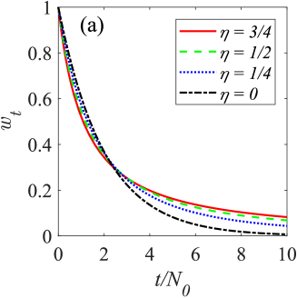
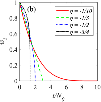
Figure 1: (Color online) The coefficient $w_{t}$ as a function of $t/N_{0}$ for networks that evolve under a combination of growth via random node addition and random attachment and contraction via random node deletion for (a) $0\leq\eta<1$; and (b) $-1<\eta<0$, obtained from Eqs. (24)-(25), where $r$ is given by Eq. (22). In case that $\eta\geq 0$ the coefficient $w_{t}$ decreases monotonically as a function of $t$ but converges towards $0$ only asymptotically. In case that $\eta<0$ the coefficient $w_{t}$ vanishes at a finite time $t_{\rm vanish}=N_{0}/|\eta|$. The curve of $w_{t}$ vs. $t/N_{0}$ is convex for $-1/3<\eta<0$ and concave for $-1<\eta<-1/3$.

For $-1<\eta<0$ the weight $w_{t}$ can be expressed in the form

$$w_{t}=\left(1-\frac{t}{t_{\rm vanish}}\right)^{\frac{1-|\eta|}{2|\eta|}}.$$ (27)

In this range the time derivative of $w_{t}$ is given by

$$\frac{dw_{t}}{dt}=-\frac{1-|\eta|}{2|\eta|t_{\rm vanish}}\left(1-\frac{t}{t_{\rm vanish}}\right)^{\frac{1-3|\eta|}{2|\eta|}}.$$ (28)

This derivative represents the rate at which the memory of the initial network is lost. For $-1/3<\eta<0$ the exponent in Eq. (28) is positive, while for $-1<\eta<-1/3$ it is negative. Therefore, as $\eta$ crosses $-1/3$ the derivative $dw_{t}/dt|_{t=t_{\rm vanish}}$ changes discontinuously from $0$ to $-\infty$. Such discontinuous changes represent a typical behavior at a phase transition.

In Fig. 2 we present the coefficient $w_{t}$ as a function of $t/t_{\rm vanish}$ for networks that evolve under a combination of growth (via random node addition and random attachment) and contraction (via random node deletion) for $-1<\eta<0$. As $t\rightarrow t_{\rm vanish}$ the slope $dw_{t}/dt$ vanishes for $-1/3<\eta<0$ and diverges for $-1<\eta<-1/3$.

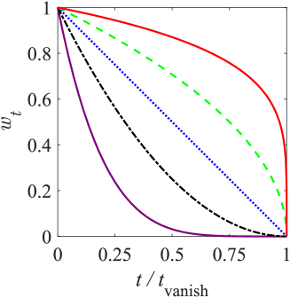
Figure 2: (Color online) The coefficient $w_{t}$ as a function of $t/t_{\rm vanish}$ for networks that evolve under a combination of growth via random node addition and random attachment and contraction via random node deletion for $\eta=-1/11$, $-1/5$, $-1/3$, $-1/2$ and $-5/7$ (from left to right), obtained from Eq. (27), which is valid for $\eta<0$. The curve of $w_{t}$ vs. $t/N_{0}$ is convex for $-1/3<\eta<0$ and concave for $-1<\eta<-1/3$, while for $\eta=-1/3$ it follows a straight line.

As time evolves, the first term in Eq. (23) decreases while the second term increases and flows towards an asymptotic state, given by

$$G_{\rm st}(u)=r\int_{0}^{1}y^{r-1}e^{-2rm(1-u)(1-y)}dy.$$ (29)

Expressing the integral in terms of the lower incomplete gamma function $\gamma(s,x)$, given by Eq. (57) in Appendix A, we obtain

$$G_{\rm st}(u)=re^{-2rm(1-u)}[-2rm(1-u)]^{-r}\gamma[r,-2rm(1-u)].$$ (30)

Using this notation, one can express Eq. (23) in the form

$$G_{t}(u) = \alpha_{t}^{r}e^{-2rm(1-\alpha_{t})(1-u)}G_{0}[1-\alpha_{t}(1-u)]$$ (31)

$$+ \left\{1-\frac{\gamma[r,-2rm\alpha_{t}(1-u)]}{\gamma[r,-2rm(1-u)]}\right\}G_{\rm st}(u),$$

where the first term captures the memory of the degree distribution of the initial network while the second term includes the components that do not depend on the initial degree distribution. As time evolves, the first term decays while the second term converges towards the asymptotic form, given by Eq. (30).

V The degree distribution

In Appendix A we extract the time dependent degree distribution $P_{t}(k)$ from the generating function $G_{t}(u)$. It is given by

$$P_{t}(k) = \alpha_{t}^{r}\frac{e^{-2rm(1-\alpha_{t})}}{k!}\sum_{i=0}^{k}\binom{k}{i}\alpha_{t}^{i}\frac{d^{i}G_{0}(u)}{du^{i}}\bigg{|}_{u=1-\alpha_{t}}\left[2rm(1-\alpha_{t})\right]^{k-i}$$ (32)

$$+ re^{-2rm}\frac{(2rm)^{k}}{k!}\int_{\alpha_{t}}^{1}y^{r-1}e^{2rmy}(1-y)^{k}dy.$$

The dependence of $P_{t}(k)$ on the initial degree distribution $P_{0}(k)$ is captured by first term of Eq. (32), while the second term is an asymptotic solution that does not depend on the initial condition. This asymptotic solution is essentially an attractive fixed point. The rate of convergence depends on the parameter $\eta$. More precisely, it is regulated by the coefficient $w_{t}=\alpha_{t}^{r}$ which appears in front of the term that captures the initial condition. As mentioned in the previous section, the dependence of $w_{t}$ on time is different in the regime of overall network growth ($\eta>0$) and the regime of overall network contraction ($\eta<0$). For $\eta>0$ the coefficient $w_{t}$ decays asymptotically like

$$w_{t}\sim t^{-\frac{r}{r-1}}.$$ (33)

Thus, for sufficiently long times the memory of the initial degree distribution is completely lost and $P_{t}(k)$ approaches its asymptotic form.

In the case of $\eta<0$ the coefficient $w_{t}$ decays as time evolves until it vanishes at a finite time $t_{\rm vanish}$. At the point $\eta=-1/3$ there is transition from a convex shape of $w_{t}$ as a function of the time $t$ (for $-1/3<\eta<0$) to a concave shape (for $-1\leq\eta<-1/3$), as can be seen in Fig. 2. For $\eta>-1/3$, as $t\rightarrow t_{\rm vanish}$ the derivative $dw_{t}/dt\rightarrow 0$. In contrast, for $\eta<-1/3$, as $t\rightarrow t_{\rm vanish}$ the derivative $dw_{t}/dt\rightarrow-\infty$. This sharp discontinuity in $dw_{t}/dt|_{t_{\rm vanish}}$ at $\eta=-1/3$ pinpoints the location of the dynamical transition. Note that the value of $\eta=-1/3$ corresponds to the situation in which $P_{\rm add}=1/3$ and $P_{\rm del}=2/3$, namely on average there are two node deletion steps for each node addition step.

From Eq. (32) one observes that on top of the overall dependence on $w_{t}$, the rate of convergence of $P_{t}(k)$ towards its asymptotic value depends on the degree $k$. The asymptotic form of $P_{t}(k)$ in the long time limit can be obtained by inserting $\alpha_{t}=0$ in Eq. (32). It yields

$$P_{\rm st}(k)=re^{-2rm}\frac{(2rm)^{k}}{k!}\int_{0}^{1}y^{r-1}e^{2rmy}(1-y)^{k}dy.$$ (34)

The right hand side of Eq. (34) can be expressed in the form

$$P_{\rm st}(k)=e^{-2rm}\frac{(2rm)^{k}}{k!}rB(k+1,r)\ _{1}F_{1}\left(\begin{array}[]{c}r\\ k+r+1\end{array}\bigg{|}2rm\right),$$ (35)

where $B(m,n)$ is the beta function and ${}_{1}F_{1}(\cdot)$ is the confluent hypergeometric function [64].

The tail of the steady state degree distribution $P_{\rm st}(k)$, where $k\gg r$ can be reduced to

$$P_{\rm st}(k)\simeq\Gamma(r+1)k^{-r}e^{-2rm}\frac{(2rm)^{k}}{k!}.$$ (36)

This tail resembles the Poisson distribution in the sense that it satisfies the condition that $P_{\rm st}(k)/P_{\rm st}(k-1)\propto 1/k$.

In the special case of $\eta=0$ (where $r=1$), which represents a perfect balance between the growth and contraction processes, the distribution $P_{\rm st}(k)$ takes a particularly simple form

$$P_{\rm st}(k;\eta=0)=\frac{1}{2m}\left[1-\frac{\Gamma(k+1,2m)}{\Gamma(k+1)}\right],$$ (37)

where $\Gamma(s,x)$ is the upper incomplete gamma function, which can be expressed in terms of the lower incomplete gamma function, in the form $\Gamma(s,x)=\Gamma(s)-\gamma(s,x)$. The steady state degree distribution for the special case of balanced growth and contraction was calculated in Ref. [58] for a slightly different model. The degree distribution $P_{\rm st}(k;\eta=0)$, given by Eq. (37), resembles the degree distribution presented in Eq. (20) of Ref. [58]. The difference in the pre-factors reflects the variation in the details of the growth mechanism between the two models.

The discontinuity in the derivative $dw_{t}/dt|_{t_{\rm vanish}}$ across $\eta=-1/3$ has interesting implications on the evolution of the degree distribution $P_{t}(k)$ in the late stages of the contraction process. For $\eta>-1/3$ there is a significant time window in which $w_{t}$ is small and thus the time dependent degree distribution $P_{t}(k)$ is in the vicinity of $P_{\rm st}(k)$. In contrast, for $\eta<-1/3$ the weight $w_{t}$ decreases slowly until the very late stages of the contraction process and then falls down sharply as the time $t_{\rm vanish}$ is approached. Therefore, there is only an extremely short time window in which $P_{t}(k)$ is in the vicinity of $P_{\rm st}(k)$.

As discussed in Sec. IV, the case of $\eta=1$ corresponds to a singular point of the equation for the generating function $G_{t}(u)$ [Eq. (21)]. Therefore, this case requires a special treatment. In Appendix B we solve the master equation for the special case of pure growth ($\eta=1$) and obtain the time dependent degree distribution $P_{t}(k)$ in this case too. It is given by

$$P_{t}(k;\eta=1) = \beta_{t}^{2m+1}P_{0}(k)+\sum_{i=1}^{k}\frac{\beta_{t}^{2m+1}}{i!}(-2m\ln\beta_{t})^{i}\left[P_{0}(k-i)-P_{\rm st}(k-i;\eta=1)\right]$$ (38)

$$+ \left(1-\beta_{t}^{2m+1}\right)P_{\rm st}(k;\eta=1),$$

where $\beta_{t}$ is given by Eq. (80) and

$$P_{\rm st}(k;\eta=1)=\frac{1}{2m+1}\left(\frac{2m}{2m+1}\right)^{k}$$ (39)

is the steady state degree distribution obtained at long times. Comparing Eq. (36) to Eq. (39) describing the degree distribution in the case of pure growth, we conclude that there is a phase transition at $\eta=1$. In the case of pure growth ($\eta=1$) the degree distribution follows an exponential distribution, whose tail decays more slowly than Eq. (36) that applies in the range of $-1<\eta<1$.

Consider the special case in which the initial network is generated using the random attachment model. This model is obtained by choosing $\eta=1$, where the number of edges added in each growth step is denoted by $m_{0}$ until the network size reaches $N_{0}$ nodes. Using the results of Appendix B, it is found that for a sufficiently large network size $N_{0}$ the generating function of the resulting network converges towards its steady state form, which is given by

$$G_{0}(u)=\frac{1}{2m_{0}(1-u)+1}.$$ (40)

The initial network is then exposed to a combination of node addition with random attachment and random node deletion, characterized by $-1<\eta<1$, where the number of edges added in each growth step is $m$. Inserting $G_{0}(u)$ from Eq. (40) into Eq. (32) and carrying out the differentiation, we obtain

$$P_{t}(k) = \alpha_{t}^{r}\frac{e^{-2rm(1-\alpha_{t})}}{2m_{0}\alpha_{t}+1}\sum_{i=0}^{k}\left(\frac{2m_{0}\alpha_{t}}{2m_{0}\alpha_{t}+1}\right)^{i}\frac{\left[2rm(1-\alpha_{t})\right]^{k-i}}{(k-i)!}$$ (41)

$$+ re^{-2rm}\frac{(2rm)^{k}}{k!}\int_{\alpha_{t}}^{1}y^{r-1}e^{2rmy}(1-y)^{k}dy.$$

Interestingly, the sum in Eq. (41) takes the form of a convolution between an exponential distribution and a Poisson distribution. The mean of the exponential distribution is equal to $2m_{0}\alpha_{t}$, while the mean of the Poisson distribution is $2rm(1-\alpha_{t})$. The exponential distribution descends from the intial degree distribution, which is given by Eq. (39), while the Poisson distribution emerges from the dynamics of the attachment and deletion processes. The Poisson distribution describes the degree distribution of an Erdős-Rényi network, which is a maximal entropy network with a given value of the mean degree. Therefore, the Poisson distribution in Eq. (41) reflects the randomization of the degrees as the network evolves in time.

Consider the case in which the initial network is an Erdős-Rényi network with mean degree $c$, whose degree distribution is known to be a Poisson distribution. In this case the time-dependent degree distribution takes a particularly simple form, namely

$$P_{t}(k) = \alpha_{t}^{r}e^{-[\alpha_{t}c+2rm(1-\alpha_{t})]}\frac{\left[\alpha_{t}c+2rm(1-\alpha_{t})\right]^{k}}{k!}$$ (42)

$$+ re^{-2rm}\frac{(2rm)^{k}}{k!}\int_{\alpha_{t}}^{1}y^{r-1}e^{2rmy}(1-y)^{k}dy.$$

The first term in Eq. (42) represents a Poisson distribution whose mean degree evolves in time, extrapolating between the initial value of the mean degree, $c$, and a final value of $2rm$. The second term does not depend on the initial network and is identical to the corresponding term that is obtained for other initial conditions. In this case the initial network is a maximal entropy network. For overall network contraction, under conditions of sufficiently high deletion rate ($-1<\eta<-1/3$) the first term of Eq. (42) maintains this property for a long time window with a decreasing mean degree. This resembles the behavior in the limit of pure network contraction, discussed in Refs. [48, 49].

In Fig. 3 we present analytical results (solid line), obtained from Eq. (39), for the steady-state degree distribution $P_{\rm st}(k)$ of networks that evolve under conditions of pure growth ($\eta=1$) via node addition and random attachment with $m=4$. To examine the convergence towards the steady-state degree distribution, we also present simulation results (circles) for the time-dependent degree distribution $P_{t}(k)$ for a network grown from an initial ER network of size $N_{0}=100$ with mean degree $c=3$ up to a size of $N=10^{4}$. The tail of the degree distribution obtained from the simulations deviates from the steady state distribution. This deviation is due to the slow convergence of $P_{t}(k)$ towards $P_{\rm st}(k)$ in the case $\eta=1$. This conclusion is supported by the very good agreement between the simulation results (circles) and the corresponding analytical results (dashed line) for $P_{t}(k)$ at $t=N-N_{0}$, obtained from Eq. (38).

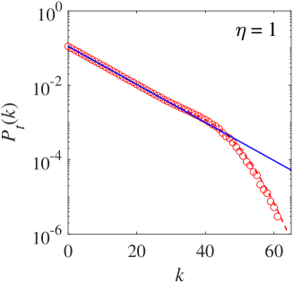
Figure 3: (Color online) Analytical results (solid line) for the asymptotic degree distribution $P_{\rm st}(k)$ of networks that evolves under conditions of pure growth ($\eta=1$) via node addition and random attachment with $m=4$, obtained from Eq. (39). To examine the convergence towards the steady state, we also present simulation results (circles) for the time dependent degree distribution $P_{t}(k)$ for a network grown from an initial ER network of size $N_{0}=100$ with mean degree $c=3$ up to a size of $N=10^{4}$. The tail of the degree distribution obtained from the simulations deviates from the steady state distribution. This deviation is due to the slow convergence of $P_{t}(k)$ towards $P_{\rm st}(k)$ in the case $\eta=1$. This conclusion is supported by the very good agreement between the simulation results (circles) and the corresponding analytical results (dashed line) for $P_{t}(k)$ at $t=N-N_{0}$, obtained from Eq. (38).

In Fig. 4 we present analytical results (solid lines), obtained from Eq. (35), for the steady-state degree distributions $P_{\rm st}(k)$ of networks that evolve under a combination of growth (via node addition and random attachment) and contraction (via random node deletion) in the regime of overall network growth ($0<\eta<1$). Results are presented for (a) $\eta=3/4$, (b) $\eta=1/2$ and (c) $\eta=1/4$. We also present simulation results (circles), which are shown for $N=10,000$. The initial network used in the simulations is an ER network of size $N_{0}=100$ with mean degree $c=3$. In the case of $\eta=1/2$ and $\eta=1/4$ the analytical results are in very good agreement with the simulation results, which means that the degree distribution in the simulation has already converged to its steady-state form $P_{\rm st}(k)$. In the case of $\eta=3/4$ one finds that at $N=10,000$ the tail of the degree distribution $P_{t}(k)$ deviates from the steady-state distribution $P_{\rm st}(k)$. This deviation is due to the slow convergence of $P_{t}(k)$ as $\eta$ is increased towards $1$. To justify this conclusion, we also present analytical results (dashed line) for $P_{t}(k)$, obtained from Eq. (42) at $t=(N-N_{0})/\eta$, which are in very good agreement with the simulation results (circles).

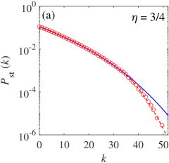
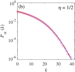
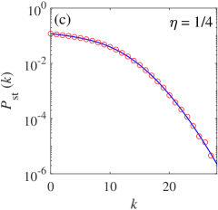
Figure 4: (Color online) Analytical results (solid lines), obtained from Eq. (35), for the steady-state degree distributions $P_{\rm st}(k)$ of networks that evolve under a combination of growth (via node addition and random attachment) and contraction (via random node deletion) in the regime of overall network growth ($0<\eta<1$). Results are presented for (a) $\eta=3/4$, (b) $\eta=1/2$ and (c) $\eta=1/4$. We also present simulation results (circles), which are shown for $N=10,000$. The initial network used in the simulations is an ER network of size $N_{0}=100$ with mean degree $c=3$. In the case of $\eta=1/2$ and $\eta=1/4$ the analytical results are in very good agreement with the simulation results, which means that the degree distribution in the simulation has already converged to its steady-state form $P_{\rm st}(k)$. In the case of $\eta=3/4$ one finds that at $N=10,000$ the tail of the degree distribution $P_{t}(k)$ deviates from the steady-state distribution $P_{\rm st}(k)$. This deviation is due to the slow convergence of $P_{t}(k)$ as $\eta$ is increased towards $1$. To justify this conclusion, we also present analytical results (dashed line) for $P_{t}(k)$, obtained from Eq. (42) at $t=(N-N_{0})/\eta$, which are in very good agreement with the simulation results (circles).

In Fig. 5 we present analytical results (solid lines), obtained from Eq. (37), for the steady-state degree distribution $P_{\rm st}(k)$ of networks that evolve under a combination of growth (via node addition and random attachment) and contraction (via random node deletion), in the special case of $\eta=0$ in which the network size is fixed, apart from possible fluctuations. We also present simulation results (circles). The initial network is an ER network of size $N_{0}=10^{4}$ with mean degree $c=3$. The analytical results are in very good agreement with the simulation results (circles), which are shown for $t=6N_{0}$, where the degree distribution has already converged to its asymptotic form $P_{\rm st}(k)$.

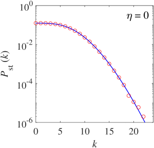
Figure 5: (Color online) Analytical results (solid lines) for the asymptotic degree distributions $P_{\rm st}(k)$ of networks that evolve under a combination of growth (via node addition and random attachment) and contraction (via random node deletion) in the special case of $\eta=0$ in which the network size is fixed, apart from possible fluctuations. The initial network is an ER network of size $N_{0}=10^{4}$ with mean degree $c=3$. The analytical results for $P_{\rm st}(k)$ are obtained from Eq. (37). The analytical results are in very good agreement with the simulation results (circles), which are shown for $t=6N_{0}$, where the degree distribution has already converged to its asymptotic form $P_{\rm st}(k)$.

In Fig. 6 we present analytical results (solid lines) for the time-dependent degree distributions $P_{t}(k)$ of networks that evolve under a combination of growth (via node addition and random attachment) and contraction (via random node deletion) in the regime of overall network contraction for (a) $\eta=-1/4$, (b) $\eta=-1/2$ and (c) $\eta=-3/4$. In each frame the degree distribution $P_{t}(k)$, obtained from Eq. (41), is shown (right to left) for $\tau=0$, $\tau=1/4$, $\tau=1/2$ and $\tau=3/4$, where the normalized time $\tau$ is the fraction of nodes that have been deleted [Eq. (5)]. The long-time degree distribution $P_{\rm st}(k)$, obtained from Eq. (35), is also shown (dashed lines). The initial condition at $t=0$ is a network obtained from random node addition and random attachment with $m_{0}=8$ and it consists of $N=12,500$ nodes. Thus, the initial degree distribution $P_{0}(k)$ is given by Eq. (39), with $m$ replaced by $m_{0}$. The simulation results (circles) are in very good agreement with the corresponding analytical results. As time evolves the time dependent degree distribution $P_{t}(k)$ converges towards the asymptotic distribution $P_{\rm st}(k)$. For $\eta=-1/4$ the degree distribution $P_{t}(k)$ approaches $P_{\rm st}(k)$ when a significant fraction of the network is still in place. In contrast, for $\eta=-1/2$ and $-3/4$ the convergence of $P_{t}(k)$ is initially very slow and it gets closer to $P_{\rm st}(k)$ only shortly before the network vanishes. The transition between the two dynamical behaviors takes place at $\eta=-1/3$.

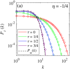
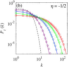
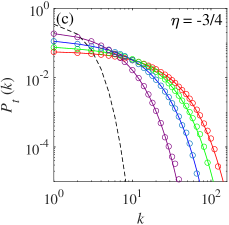
Figure 6: (Color online) Analytical results (solid lines) for the degree distributions of networks that evolve under a combination of growth via random node addition and random attachment and contraction via random node deletion in the regime of overall network contraction for (a) $\eta=-1/4$, (b) $\eta=-1/2$ and (c) $\eta=-3/4$. In each frame the degree distribution $P_{t}(k)$ is shown (right to left) for $\tau=0$, $\tau=1/4$, $\tau=1/2$ and $\tau=3/4$, where the normalized time $\tau$ is the fraction of nodes that have been deleted [Eq. (5)]. The asymptotic distribution $P_{\rm st}(k)$ is also shown (dashed lines). The initial network is obtained from random node addition and random attachment with $m_{0}=8$ and it consists of $N_{0}=12,500$ nodes. The analytical results for $P_{t}(k)$, are obtained from Eq. (41). The simulation results (circles) are in very good agreement with the corresponding analytical results. As time evolves the time dependent degree distribution $P_{t}(k)$ converges towards the asymptotic distribution $P_{\rm st}(k)$. For $\eta=-1/4$, the degree distribution $P_{t}(k)$ approaches $P_{\rm st}(k)$ when a significant fraction of the network is still in place. In contrast, for $\eta=-1/2$ and $-3/4$ the convergence of $P_{t}(k)$ is initially very slow and it gets closer to $P_{\rm st}(k)$ only shortly before the network vanishes. The transition between the two dynamical behaviors takes place at $\eta=-1/3$.

VI The mean and variance of the degree distribution

The mean degree at time $t$ can be obtained from

$$\langle K\rangle_{t}=\frac{d}{du}G_{t}(u)\bigg{|}_{u=1}.$$ (43)

Inserting $G_{t}(u)$ from Eq. (23) into Eq. (43), we obtain

$$\langle K\rangle_{t}=\alpha_{t}^{r+1}\langle K\rangle_{0}+(1-\alpha_{t}^{r+1})\langle K\rangle_{\rm st},$$ (44)

where

$$\langle K\rangle_{\rm st}=\frac{2rm}{r+1}.$$ (45)

In Fig. 7 we present analytical results (solid lines), obtained from Eq. (44), for the mean degree $\langle K\rangle_{t}$ vs. time $t$ for networks that evolve under a combination of growth (via node addition and random attachment) and contraction (via random node deletion) for (a) $0\leq\eta<1$; and (b) $-1<\eta<0$. The mean degree of the initial network is $\langle K\rangle_{0}=16$. In case that $\eta>0$ the mean degree gradually converges towards its asymptotic value. In case that $\eta<0$ the network vanishes at a finite time $t_{\rm vanish}=N_{0}/|\eta|$.

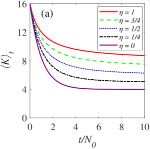
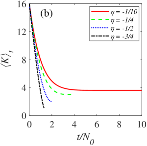
Figure 7: (Color online) Analytical results (solid lines), obtained from Eq. (44), for the mean degree $\langle K\rangle_{t}$ vs. time $t$ for networks that evolve under a combination of growth (via node addition and random attachment) and contraction (via random node deletion) for (a) $\eta=1$, $3/4$, $1/2$, $1/4$ and $0$ (from top to bottom); and (b) $\eta=-1/10$, $-1/4$, $-1/2$ and $-3/4$ (from top to bottom). In all cases the initial network has a mean degree of $\langle K\rangle_{0}=16$. In case that $\eta>0$ the mean degree gradually converges towards its asymptotic value. In case that $\eta<0$ the network vanishes at a finite time $t_{\rm vanish}=N_{0}/|\eta|$.

In Fig. 8 we present analytical results (solid lines), for the mean degree $\langle K\rangle_{t}$ vs. $t/t_{\rm vanish}$ for networks that evolve under a combination of growth (via node addition and random attachment) and contraction (via random node deletion) for $-1<\eta<0$.

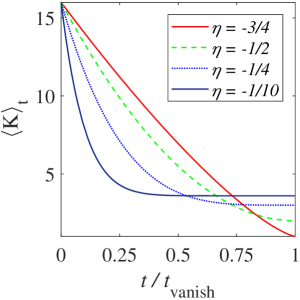
Figure 8: (Color online) Analytical results (solid lines), obtained from Eq. (44), for the mean degree $\langle K\rangle_{t}$ vs. $t/t_{\rm vanish}$ for networks that evolve under a combination of growth (via node addition and random attachment) and contraction (via random node deletion) for $\eta=-3/4$, $-1/2$, $-1/4$ and $-1/10$ (from top to bottom). The initial network has a mean degree of $\langle K\rangle_{0}=16$.

To obtain the variance ${\rm Var}_{t}(K)$ we use the cumulant generating function, which is given by

$$F_{t}(x)=\ln G_{t}(e^{x}).$$ (46)

The variance is obtained from

$${\rm Var}_{t}(K)=\frac{d^{2}}{dx^{2}}F_{t}(x)\bigg{|}_{x=0}.$$ (47)

Inserting $F_{t}(x)$ from Eq. (46) into Eq. (47) we obtain

$${\rm Var}_{t}(K) = \alpha_{t}^{r+2}{\rm Var}_{0}(K)+\alpha_{t}^{r+1}\left[(\alpha_{t}-1)\langle K\rangle_{0}^{2}+(\alpha_{t}^{r+1}-2\alpha_{t}+1)\langle K\rangle_{0}\right]$$ (48)

$$- \alpha_{t}^{r+1}(\alpha_{t}^{r+1}-1)\left(\langle K\rangle_{0}-\langle K\rangle_{\rm st}\right)^{2}$$

$$+ 2\alpha_{t}^{r+1}(\alpha_{t}-1)(r+1)\left[\frac{r+1}{r+2}\langle K\rangle_{\rm st}-\langle K\rangle_{0}\right]\langle K\rangle_{\rm st}$$

$$+ (1-\alpha_{t}^{r+1}){\rm Var}_{\rm st}(K),$$

where

$${\rm Var}_{\rm st}(K)=\frac{2rm[(2m+1)r^{2}+3r+2]}{(r+1)^{2}(r+2)}$$ (49)

is the variance of $P_{\rm st}(k)$, given by Eq. (35). Note that at $t=0$ the right hand side of Eq. (48) is reduced to ${\rm Var}_{0}(K)$ while in the long time limit it converges towards ${\rm Var}_{\rm st}(K)$.

The mean $\langle K\rangle_{t}(\eta=1)$ and variance ${\rm Var}_{t}(K;\eta=1)$ of the degree distribution $P_{t}(k;\eta=1)$ in the case of $\eta=1$ are calculated in Appendix B. The steady state results $\langle K\rangle_{\rm st}(\eta=1)$ and ${\rm Var}_{\rm st}(K;\eta=1)$ coincide with those obtained from $\langle K\rangle_{t}$ and ${\rm Var}_{t}(K)$, respectively, in the limit of $\eta\rightarrow 1$ ($r\rightarrow\infty$).

VII Summary and Discussion

We presented analytical results for the time-dependent degree distribution $P_{t}(k)$ of networks that evolve under the combination of growth (via node addition and random attachment) and contraction (via random node deletion). In case that the rate of node addition exceeds the rate of node deletion, the overall process is of network growth, while in the opposite case the overall process is of network contraction. Using the master equation and the generating function formalism we obtained a closed form expression for the degree distribution $P_{t}(k)$. It includes a term that depends on the initial condition $P_{0}(k)$, which decays as time evolves, and a long-time asymptotic term $P_{\rm st}(k)$, which is an attractive fixed point. Interestingly, the expression for $P_{t}(k)$ is identical in the regimes of overall growth and overall contraction.

The model of network growth via node addition and random attachment can be considered as the simplest network growth model. It gives rise to networks that exhibit an exponential degree distribution. Similarly, the model of network contraction via random node deletion can be considered as the simplest network contraction model. The contracting networks converge towards the ER structure, which exhibits a Poisson degree distribution whose mean degree decreases as time proceeds. The combination of growth via node addition and random attachment and contraction via random node deletion yields novel structures which depend on the balance between the rates of the two processes.

In Fig. 9 we present the phase diagram of networks that evolve under a combination of growth (via node addition and random attachment) and contraction (via random node deletion), in terms of the growth rate $-1\leq\eta\leq 1$. The case of $\eta=1$ represents pure network growth via node addition and random attachment. The case of $0<\eta<1$ represents a combination of growth and contraction where the overall process is of network growth. The case of $\eta=0$ represents a balance between the growth and contraction processes such that on average the network size remains fixed. The case of $-1<\eta<0$ represents a combination of growth and contraction where the overall process is of network contraction. The case of $\eta=-1$ corresponds to pure contraction via random node deletion.

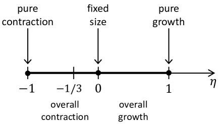
Figure 9: The phase diagram of networks that evolve under a combination of growth via random node addition and random attachment and contraction via random node deletion, in terms of the growth rate $-1\leq\eta\leq 1$. The case of $\eta=1$ represents pure network growth via node addition and random attachment. The case of $0<\eta<1$ represents a combination of growth and contraction where the overall process is of network growth. The case of $\eta=0$ represents a balance between the growth and contraction processes such that on average the network size remains fixed. The case of $-1<\eta<0$ represents a combination of growth and contraction where the overall process is of network contraction. The case of $\eta=-1$ corresponds to pure contraction via random node deletion. At $\eta=1$ there is a structural phase transition between the exponential degree distribution in the asymptotic state for $\eta=1$ and the asymptotic Poisson-like degree distribution in the regime of $0<\eta<1$, whose tail decays faster than the exponential distribution. At $\eta=0$ there is a phase transition between the $\eta>0$ phase which exhibits an ever growing network whose degree distribution converges to an asymptotic form and the $\eta<0$ phase in which the network vanishes after a finite time $t_{\rm vanish}$. At $\eta=-1/3$ there is a dynamical transition. For $-1/3<\eta<0$ the degree distribution $P_{t}(k)$ quickly converges towards $P_{\rm st}(k)$. In contrast, for $-1<\eta<-1/3$ the convergence of $P_{t}(k)$ is initially very slow and it gets closer to $P_{\rm st}(k)$ only shortly before the network vanishes.

At $\eta=1$ there is a structural phase transition between the steady-state degree distribution at $\eta=1$, which follows an exponential distribution, given by Eq. (39), and the steady-state degree distribution in the regime of $0<\eta<1$, given by Eq. (35), which decays like a Poisson distribution. This degree distribution essentially consists of a linear combination of Poisson distributions. Its tail is dominated by the Poisson component with the largest mean degree, given by Eq. (36). This transition implies that even the slightest rate of node deletion leads to a qualitative change in the nature of the steady state degree distribution. From a technical point of view, $\eta=1$ is a singular point in the differential equation (21) for the generating function $G_{t}(u)$, where the order of the equation changes. The phase transition at $\eta=1$ essentially emanates from this singularity.

At $\eta=0$ there is a phase transition between the $\eta>0$ phase which exhibits an ever growing network and the $\eta<0$ phase in which the network vanishes after a finite time. Surprisingly, the expression for the time dependent degree distribution $P_{t}(k)$, given by Eq. (41), is identical on both sides of the transition. However, the qualitative behavior of the coefficient $\alpha_{t}$ is fundamentally different on both sides. For $\eta>0$ the coefficient $\alpha_{t}$ gradually decays as time evolves but remains positive at any finite time. In contrast, for $\eta<0$ it decays to zero after a finite time $t_{\rm vanish}$, at which the whole network vanishes.

At $\eta=-1/3$ there is a dynamical transition between a phase of slow network contraction for $-1/3<\eta<0$ and a fast contracting phase for $-1\leq\eta<-1/3$. In the phase of slow contraction the degree distribution converges towards $P_{\rm st}(k)$ and remains in its vicinity for a finite time window, before the network vanishes. In the fast contracting phase the network size quickly decreases and it vanishes before the weight of $P_{\rm st}(k)$ becomes significant. In this case, the evolution of the degree distribution $P_{t}(k)$ during the contraction process qualitatively resembles the case of pure network contraction via random node deletion ($\eta=-1$), considered in Refs. [48, 49].

The behavior of the degree distribution $P_{t}(k)$ in the scenario of overall network contraction $-1<\eta<0$ can be considered in the context of dynamical processes that exhibit intermediate asymptotic states [66, 65]. These are states that appear at intermediate time scales, which are sufficiently long for such structures to build up, but shorter than the time scales at which the whole system disintegrates. The intermediate time scales can be made arbitrarily long by increasing the initial size of the system, justifying the term ‘asymptotic’. More specifically, in the regime of $-1/3<\eta<0$ the intermediate asymptotic state exhibits the degree distribution $P_{\rm st}(k)$, while in the regime of $-1\leq\eta<-1/3$ the intermediate asymptotic degree distribution is dominated by the first term of $P_{t}(k)$, given by Eq. (32).

This work was supported by grant no. 2020720 from the United States-Israel Binational Science Foundation (BSF).

Appendix A Calculation of the degree distribution $P_{t}(k)$

In this Appendix we solve the master equation [Eq. (18)] for $-1\leq\eta<1$ and obtain the time dependent degree distribution $P_{t}(k)$. In the first step we solve the differential equation (21) using the method of characteristics and obtain the time dependent generating function $G_{t}(u)$. The method of characteristics applies to hyperbolic partial differential equations. In this method the partial differential equation is reduced to a set of ordinary differential equations called characteristic equations.

The characteristic equations of Eq. (21) can be written as

$$\frac{du}{dt}=-\frac{1-\eta}{2}\frac{1-u}{N_{0}+\eta t}$$ (50)

and

$$\frac{dG_{t}(u)}{du}=\frac{1+\eta}{1-\eta}\left[\left(2m+\frac{1}{1-u}\right)G_{t}(u)-\frac{1}{1-u}\right].$$ (51)

Solving Eq. (50), one obtains a relation between $u$ and $t$, via an integration constant $C_{1}$. In the case of $\eta\neq 0$, it is given by

$$C_{1}=\frac{(1-u)^{\frac{2\eta}{1-\eta}}}{N_{0}+\eta t},$$ (52)

while in the case of $\eta=0$ it is given by

$$C_{1}=(1-u)e^{-t/2N_{0}}.$$ (53)

In order to solve Eq. (51), we express the generating function in the form

$$G_{t}(u)=G_{t}^{(h)}(u)+G_{t}^{(p)}(u),$$ (54)

where $G_{t}^{(h)}(u)$ is the homogeneous part and $G_{t}^{(p)}$ is the inhomogeneous part of $G_{t}(u)$. Solving for the homogeneous part, we obtain

$$G_{t}^{(h)}(u)=C_{2}e^{2rmu}(1-u)^{-r},$$ (55)

where $C_{2}$ is an integration constant, and $r$ is defined in Eq. (22). Solving Eq. (51) for the inhomogeneous part of $G_{t}(u)$, we obtain

$$G_{t}^{(p)}(u)=re^{-2rm(1-u)}\frac{\gamma[r,-2rm(1-u)]}{[-2rm(1-u)]^{r}},$$ (56)

where

$$\gamma(s,x)=\int_{0}^{x}t^{s-1}e^{-t}dt$$ (57)

is the lower incomplete gamma function [64]. Inserting $G_{t}^{(h)}(u)$ from Eq. (55) and $G_{t}^{(p)}(u)$ from Eq. (56) into Eq. (54) and extracting the integration constant $C_{2}$, we obtain

$$C_{2}=e^{-2rmu}(1-u)^{r}G_{t}(u)-re^{-2rm}(1-u)^{r}\frac{\gamma[r,-2rm(1-u)]}{(-2rm)^{r}}.$$ (58)

Starting with the case of $\eta\neq 0$, we combine the solutions of the two characteristic equations and obtain the solution of Eq. (21), which is given by

$$G_{t}(u)=e^{2rmu}(1-u)^{-r}F\left[\frac{(1-u)^{\frac{2\eta}{1-\eta}}}{N_{0}+\eta t}\right]+re^{-2rm(1-u)}\frac{\gamma[r,-2rm(1-u)]}{[-2rm(1-u)]^{r}},$$ (59)

where $F$ is an arbitrary function. In order to impose the initial condition $G_{0}(u)$ we set $t=0$ in Eq. (59) and obtain

$$G_{0}(u)=e^{2rmu}(1-u)^{-r}F\left[\frac{(1-u)^{\frac{2\eta}{1-\eta}}}{N_{0}}\right]+re^{-2rm(1-u)}\frac{\gamma[r,-2rm(1-u)]}{[-2rm(1-u)]^{r}}.$$ (60)

Solving for the arbitrary function $F$, we obtain

$$F\left[\frac{(1-u)^{\frac{2\eta}{1-\eta}}}{N_{0}}\right]=e^{-2rmu}(1-u)^{r}G_{0}(u)-re^{-2rm}\frac{\gamma[r,-2rm(1-u)]}{(-2rm)^{r}}.$$ (61)

We introduce the variable

$$z=\frac{(1-u)^{\frac{2\eta}{1-\eta}}}{N_{0}}.$$ (62)

Expressing $u$ in terms of $z$, we obtain

$$u=1-(zN_{0})^{\frac{1-\eta}{2\eta}}.$$ (63)

Rewriting Eq. (61) in terms of the variable $z$, we obtain

$$F(z) = e^{-2rm\left[1-(zN_{0})^{\frac{1-\eta}{2\eta}}\right]}(zN_{0})^{\frac{r(1-\eta)}{2\eta}}G_{0}\left[1-(zN_{0})^{\frac{1-\eta}{2\eta}}\right]$$ (64)

$$- re^{-2rm}\frac{\gamma\left[r,-2rm(zN_{0})^{\frac{1-\eta}{2\eta}}\right]}{(-2rm)^{r}}.$$

Inserting $F(z)$ from Eq. (64) into Eq. (59), we obtain

$$G_{t}(u) = \alpha_{t}^{r}e^{-2rm(1-u)(1-\alpha_{t})}G_{0}[1-\alpha_{t}(1-u)]$$ (65)

$$+ re^{-2rm(1-u)}\frac{\gamma[r,-2rm(1-u)]-\gamma[r,-2rm\alpha_{t}(1-u)]}{[-2rm(1-u)]^{r}},$$

where

$$\alpha_{t}=\left(1+\frac{\eta t}{N_{0}}\right)^{-\frac{1-\eta}{2\eta}}.$$ (66)

A similar analysis applies to the special case of $\eta=0$. In this case one needs to use the special expression for $C_{1}$, given by Eq. (53). It yields the same form of $G_{t}(u)$, given by Eq. (65), but with a different expression for $\alpha_{t}$, which in the case of $\eta=0$ is given by

$$\alpha_{t}=\exp\left(-\frac{t}{2N_{0}}\right).$$ (67)

To simplify Eq. (65) we first denote

$$S(u)=\gamma[r,-2rm(1-u)]-\gamma[r,-2rm\alpha_{t}(1-u)].$$ (68)

Replacing $\gamma(s,x)$ by its integral representation (57), one can express $S(u)$ in the form

$$S(u)=\int_{-2rm\alpha_{t}(1-u)}^{-2rm(1-u)}x^{r-1}e^{-x}dx.$$ (69)

Substituting $x=-2rm(1-u)y$ in Eq. (69), we obtain

$$S(u)=[-2rm(1-u)]^{r}\int_{\alpha_{t}}^{1}y^{r-1}e^{2rm(1-u)y}dy.$$ (70)

Plugging $S(u)$ from Eq. (70) into Eq. (65), one obtains

$$G_{t}(u) = \alpha_{t}^{r}e^{-2rm(1-u)(1-\alpha_{t})}G_{0}[1-\alpha_{t}(1-u)]$$ (71)

$$+ r\int_{\alpha_{t}}^{1}y^{r-1}e^{-2rm(1-u)(1-y)}dy.$$

The time dependent degree distribution is obtained by differentiating the generating function $G_{t}(u)$:

$$P_{t}(k)=\frac{1}{k!}\frac{\partial^{k}G_{t}(u)}{\partial u^{k}}\bigg{|}_{u=0}.$$ (72)

Inserting $G_{t}(u)$ from Eq. (71) into Eq. (72), we obtain the main result of this Appendix, namely

$$P_{t}(k) = \alpha_{t}^{r}\frac{e^{-2rm(1-\alpha_{t})}}{k!}\sum_{i=0}^{k}\binom{k}{i}\alpha_{t}^{i}\frac{d^{i}G_{0}(u)}{du^{i}}\bigg{|}_{u=1-\alpha_{t}}\left[2rm(1-\alpha_{t})\right]^{k-i}$$ (73)

$$+ re^{-2rm}\frac{(2rm)^{k}}{k!}\int_{\alpha_{t}}^{1}y^{r-1}e^{2rmy}(1-y)^{k}dy.$$

This is a closed form analytical expression for the time dependent degree distribution $P_{t}(k)$. It is based on the initial degree distribution $P_{0}(k)$, which is encoded in the generating function at time $t=0$, $G_{0}(u)$.

Appendix B Calculation of $P_{t}(k)$ in the case of pure network growth

The case of pure network growth via node addition and random attachment is obtained for $\eta=1$. Inserting $\eta=1$ in Eq. (21), we obtain

$$(N_{0}+t)\frac{\partial G_{t}(u;\eta=1)}{\partial t}=-\left[2m(1-u)+1\right]G_{t}(u;\eta=1)+1.$$ (74)

The characteristic equations in this case are given by

$$\frac{du}{dt}=0,$$ (75)

and

$$\frac{dG_{t}(u;\eta=1)}{dt}=\frac{1-[2m(1-u)+1]G_{t}(u;\eta=1)}{N_{0}+t}.$$ (76)

From Eq. (75) one finds that on the characteristic lines the variable $u$ is a constant that does not depend on time. Solving Eq. (76) it is found that

$$G_{t}(u;\eta=1)=F(u)(N_{0}+t)^{-[2m(1-u)+1]}+\frac{1}{2m(1-u)+1},$$ (77)

where $F(u)$ is a yet unknown function of $u$ that does not depend on time. Inserting $t=0$ into Eq. (77), we obtain

$$G_{0}(u)=F(u)(N_{0})^{-[2m(1-u)+1]}+\frac{1}{2m(1-u)+1}.$$ (78)

Extracting $F(u)$ from Eq. (78) and inserting it back into Eq. (77), we obtain

$$G_{t}(u;\eta=1)=\beta_{t}^{2m(1-u)+1}G_{0}(u)+\left[1-\beta_{t}^{2m(1-u)+1}\right]\frac{1}{2m(1-u)+1},$$ (79)

where

$$\beta_{t}=\left(1+\frac{t}{N_{0}}\right)^{-1}.$$ (80)

In the long time limit, the generating function converges towards a steady state of the form

$$G_{\rm st}(u;\eta=1)=\frac{1}{2m(1-u)+1}.$$ (81)

Expanding Eq. (81) in powers of $u$, we obtain the steady state degree distribution

$$P_{\rm st}(k;\eta=1)=\frac{1}{2m+1}\left(\frac{2m}{2m+1}\right)^{k},$$ (82)

which is an exponential distribution. The mean of the distribution $P_{\rm st}(k;\eta=1)$ is given by

$$\langle K\rangle_{\rm st}(\eta=1)=2m,$$ (83)

and its variance is given by

$${\rm Var}_{\rm st}(K;\eta=1)=2m(2m+1).$$ (84)

The time dependent degree distribution is obtained by expanding the right hand side of Eq. (79) in powers of $u$. It yields

$$P_{t}(k;\eta=1) = \beta_{t}^{2m+1}P_{0}(k)$$ (85)

$$+ \beta_{t}^{2m+1}\sum_{i=1}^{k}\frac{\left[2m\ln\beta_{t}\right]^{i}}{i!}\left[P_{0}(k-i)-P_{\rm st}(k-i;\eta=1)\right]$$

$$+ \left[1-\beta_{t}^{2m+1}\right]P_{\rm st}(k;\eta=1).$$

The mean degree can be obtained from Eq. (43), where $G_{t}(u;\eta=1)$ is taken from Eq. (79). It is given by

$$\langle K\rangle_{t}(\eta=1)=\beta_{t}\langle K\rangle_{0}+(1-\beta_{t})2m.$$ (86)

To obtain the variance ${\rm Var}_{t}(K)$ we use the cumulant generating function, which is given by

$$F_{t}(x;\eta=1)=\ln G_{t}(e^{x};\eta=1).$$ (87)

The variance is obtained from

$${\rm Var}_{t}(K;\eta=1)=\frac{d^{2}}{dx^{2}}F_{t}(x;\eta=1)\bigg{|}_{x=0}.$$ (88)

Inserting $F_{t}(x;\eta=1)$ from Eq. (87) into Eq. (88), one finds that

$${\rm Var}_{t}(K;\eta=1) = \beta_{t}{\rm Var}_{0}(K;\eta=1)$$ (89)

$$+ (1-\beta_{t}){\rm Var}_{\rm st}(K;\eta=1)$$

$$+ \beta_{t}(1-\beta_{t})\left[\langle K\rangle_{0}(\eta=1)-\langle K\rangle_{\rm st}(\eta=1)\right]^{2}$$

$$- 4m\beta_{t}\ln\beta_{t}\left[\langle K\rangle_{0}(\eta=1)-\langle K\rangle_{\rm st}(\eta=1)\right].$$

References

- [1] S.N. Dorogovtsev and J.F.F. Mendes, Evolution of Networks: From Biological Nets to the Internet and WWW (Oxford University Press, Oxford, 2003).
- [2] V. Latora, V. Nicosia and G. Russo, Complex Networks: Principles, Methods and Applications (Cambridge University Press, Cambridge, 2017).
- [3] S. Havlin and R. Cohen, Complex Networks: Structure, Robustness and Function (Cambridge University Press, New York, 2010).
- [4] M.E.J. Newman, Networks: an Introduction, Second Edition (Oxford University Press, Oxford, 2018).
- [5] E. Estrada, The structure of complex networks: theory and applications (Oxford University Press, Oxford, 2011).
- [6] S. Redner, How popular is your paper? An empirical study of the citation distribution, Eur. Phys. J. B 4, 131 (1998).
- [7] A.-L. Barabási and R. Albert, Emergence of scaling in random networks, Science 286, 509 (1999).
- [8] R. Albert and A.-L. Barabási, Statistical mechanics of complex networks, Rev. Mod. Phys. 74, 47 (2002).
- [9] P.L. Krapivsky, S. Redner and F. Leyvraz, Connectivity of growing random networks, Phys. Rev. Lett. 85, 4629 (2000).
- [10] S.N. Dorogovtsev, J.F.F. Mendes and A.N. Samukhin, Structure of growing networks with preferential linking, Phys. Rev. Lett. 85, 4633 (2000).
- [11] B. Bollobás, Random Graphs, Second Edition (Academic Press, London, 2001).
- [12] R. Pastor-Satorras, E. Smith and R.V. Sole, Evolving protein interaction networks through gene duplication, J. Theor. Biol. 222, 199 (2003).
- [13] F. Chung, L. Lu, T.G. Dewey, and D.J. Galas, Duplication models for biological networks, J. Comput. Biol. 10, 677 (2003).
- [14] P.L. Krapivsky and S. Redner, Network growth by copying, Phys. Rev. E 71, 036118 (2005).
- [15] I. Ispolatov, P. Krapivsky, and A. Yuryev, Duplication-divergence model of protein interaction network, Phys. Rev. E 71, 061911 (2005).
- [16] I. Ispolatov, P.L. Krapivsky, I. Mazo and A. Yuryev, Cliques and duplication–divergence network growth, New J. Phys. 7, 145 (2005).
- [17] G. Bebek, P. Berenbrink, C. Cooper, T. Friedetzky, J. Nadeau and S.C. Sahinalp, The degree distribution of the generalized duplication model, Theor. Comput. Sci. 369, 239 (2006).
- [18] R. Lambiotte, P. L. Krapivsky, U. Bhat and S. Redner, Structural transitions in dense networks, Phys. Rev. Lett. 117, 218301 (2016).
- [19] U. Bhat, P. L. Krapivsky, R. Lambiotte and S. Redner, Densification and structural transitions in networks that grow by node copying, Phys. Rev. E. 94, 062302 (2016).
- [20] C. Steinbock, O. Biham and E. Katzav, Distribution of shortest path lengths in a class of node duplication network models, Phys. Rev. E 96, 032301 (2017).
- [21] J. Török and J. Kertész, Cascading collapse of online social networks, Scientific Reports 7, 16743 (2017).
- [22] L. Lőrincz, J. Koltai, A.F. Győr and K. Takács, Collapse of an online social network: Burning social capital to create it?, Social Networks 57, 43 (2019).
- [23] R. Albalat and C. Cañestro, Evolution by gene loss, Nature Reviews Genetics 17, 379 (2016).
- [24] L. Daqing, J. Yinan, K. Rui and S. Havlin, Spatial correlation analysis of cascading failures: Congestions and Blackouts, Scientific Reports 4, 5381 (2014).
- [25] B. Schäfer, D. Witthaut, M. Timme and V. Latora, Dynamically induced cascading failures in power grids, Nature Communications 9, 1975 (2018).
- [26] R. Pastor-Satorras and A. Vespignani, Epidemic Spreading in Scale-Free Networks, Phys. Rev. Lett. 86, 3200 (2001).
- [27] R. Pastor-Satorras, C. Castellano, P. Van Mieghem and A. Vespignani, Epidemic processes in complex networks, Rev. Mod. Phys. 87, 925 (2015).
- [28] R. Pastor-Satorras and A. Vespignani, Immunization of complex networks, Phys. Rev. E 65, 036104 (2002).
- [29] J.H. Morrison and P.R. Hof, Life and death of neurons in the aging brain, Science 278, 412 (1997).
- [30] M.-T. Heemels, Neurodegenerative diseases, Nature 539, 179 (2016).
- [31] T. Arendt, M.K. Brückner, M. Morawski, C. Jäger and H.-J. Gertz, Early neurone loss in Alzheimer’s disease: cortical or subcortical?, Acta Neuropathologica Communications 3, 10 (2015).
- [32] R. Cohen, K. Erez, D. ben-Avraham and S. Havlin, Resilience of the Internet to random breakdowns, Phys. Rev. Lett. 85, 4626 (2000).
- [33] R. Cohen, K. Erez, D. ben-Avraham and S. Havlin, Breakdown of the Internet under intentional attack, Phys. Rev. Lett. 86, 3682 (2001).
- [34] R. Albert, H. Jeong and A.-L. Barabási, Error and attack tolerance of complex networks, Nature 406, 378 (2000).
- [35] J. Gao, X. Liu, D. Li and S. Havlin, Recent progress on the resilience of complex networks, Energies 8, 12187 (2015).
- [36] X. Yuan, S. Shao, H.E. Stanley and S. Havlin, How breadth of degree distribution influences network robustness: Comparing localized and random attacks, Phys. Rev. E 92, 032122 (2015).
- [37] S. Shao, X. Huang, H.E. Stanley and S. Havlin, Percolation of localized attack on complex networks, New J. Phys. 17, 023049 (2015).
- [38] S. Havlin, H.E. Stanley, A. Bashan, J. Gao and D.Y. Kenett, Percolation of interdependent network of networks, Chaos, Solitons & Fractals 72, 4 (2015).
- [39] L.M. Shekhtman, S. Shai and S. Havlin, Resilience of networks formed of interdependent modular networks, New J. Phys. 17, 123007 (2015).
- [40] L.M. Shekhtman, M.M. Danziger and S. Havlin, Recent advances on failure and recovery in networks of networks, Chaos, Solitons & Fractals 90, 28 (2016).
- [41] X. Yuan, Y. Dai, H.E. Stanley and S. Havlin, k-core percolation on complex networks: Comparing random, localized and targeted attacks, Phys. Rev. E 93, 062302 (2016).
- [42] M.A. Di Muro, C.E. La Rocca, H.E. Stanley, S. Havlin and L.A. Braunstein, Recovery of Interdependent Networks, Scientific Reports 6, 22834 (2016).
- [43] D. Vaknin, M.M. Danziger and S. Havlin, Spreading of localized attacks in spatial multiplex networks, New J. Phys. 19, 073037 (2017).
- [44] A. Braunstein, L. Dall’Asta, G. Semerjian and L. Zdeborová, Network dismantling, Proc. Natl. Acad. Sci. USA 113, 12368 (2016).
- [45] L. Zdeborová, P. Zhang and H.-J. Zhou, Fast and simple decycling and dismantling of networks, Scientific Reports 6, 37954 (2016).
- [46] M. Molloy and B.B. Reed, A critical point for random graphs with a given degree sequence, Rand. Struct. & Algo. 6, 161 (1995).
- [47] M. Molloy and B.B. Reed, The size of the largest component of a random graph on a fixed degree sequence, Combinatorics, Probability and Computing 7, 295 (1998).
- [48] I. Tishby, O. Biham and E. Katzav, Convergence towards an Erdős-Rényi graph structure in network contraction processes, Phys. Rev. E 100, 032314 (2019).
- [49] I. Tishby, O. Biham and E. Katzav, Analysis of the convergence of the degree distribution of contracting random networks towards a Poisson distribution using the relative entropy Phys. Rev. E 101, 062308 (2020).
- [50] M. Catanzaro, M. Bogu, and R. Pastor-Satorras, Generation of uncorrelated random scale-free networks, Phys. Rev. E 71, 027103 (2005).
- [51] A.C.C. Coolen, A. Annibale and E. Roberts, Generating Random Networks and Graphs (Oxford University Press, Oxford, 2017).
- [52] A. Annibale, A.C.C. Coolen, L.P. Fernandes, F. Fraternali and J. Kleinjung, Tailored graph ensembles as proxies or null models for real networks I: tools for quantifying structure. J. Phys. A 42, 485001 (2009).
- [53] E.S. Roberts, T. Schlitt and A.C.C. Coolen, Tailored graph ensembles as proxies or null models for real networks II: results on directed graphs. J. Phys. A 44, 275002 (2011).
- [54] M.E.J. Newman, S.H. Strogatz and D.J. Watts, Random graphs with arbitrary degree distributions and their applications, Phys. Rev. E 64, 026118 (2001).
- [55] P. Erdős and A. Rényi, On random graphs I, Publ. Math. Debrecen 6, 290 (1959).
- [56] P. Erdős and A. Rényi, On the evolution of random graphs, Publ. Math. Inst. Hungar. Acad. Sci. 5, 17 (1960).
- [57] P. Erdős and A. Rényi, On the evolution of random graphs II, Bull. Inst. Internat. Statist. 38, 343 (1961).
- [58] C. Moore, G. Ghoshal and M.E.J. Newman, Exact solutions for models of evolving networks with addition and deletion of nodes, Phys. Rev. E 74, 036121 (2006).
- [59] G. Ghoshal, L. Chi and A.-L. Barabási, Uncovering the role of elementary processes in network evolution, Scientific Reports 3, 2920 (2013).
- [60] H. Bauke, C. Moore, J.B. Rouquier and D. Sherrington, Topological phase transition in a network model with preferential attachment and node removal, Eur. Phys. J. B 83, 519 (2011).
- [61] N.G. van Kampen, Stochastic Processes in Physics and Chemistry, 3rd Edition (North Holland, Amsterdam, 2007).
- [62] C. Gardiner, Handbook of Stochastic Methods: for Physics, Chemistry and the Natural Sciences, 3rd edition, (Springer-Verlag, Berlin, 2004).
- [63] C.L. Phillips, H.T. Nagle and A Chakrabortty, Digital Control System: Analysis and Design, Fourth Edition (Pearson Education, Harlow, 2015).
- [64] F.W.J. Olver, D.M. Lozier, R.R. Boisvert and C.W. Clark, NIST Handbook of Mathematical Functions (Cambridge University Press, Cambridge, 2010).
- [65] G.I. Barenblatt, Scaling (Cambridge University Press, Cambridge, 2003).
- [66] G.I. Barenblatt, Scaling, self-similarity, and intermediate asymptotics (Cambridge University Press, Cambridge, 1996).