Geometric Tracking Control of Omnidirectional Multirotors in the Presence of Rotor Dynamics

Abstract

An omnidirectional multirotor has the advantageous maneuverability of decoupled translational and rotational motions, drastically superseding the traditional multirotors’ motion capability. Such maneuverability requires an omnidirectional multirotor to frequently alter the thrust amplitude and even direction, which is prone to the rotors’ settling time induced from the rotors’ own dynamics. Furthermore, the omnidirectional multirotor’s stability for tracking control in the presence of rotor dynamics has not yet been addressed. To resolve this issue, we propose a geometric tracking controller that takes the rotor dynamics into account. We show that the proposed controller yields the zero equilibrium of the error dynamics almost globally exponentially stable. The controller’s tracking performance and stability are verified in simulations. Furthermore, the single-axis force experiment with the omnidirectional multirotor has been performed to confirm the proposed controller’s performance in mitigating the rotors’ settling time in the real world.

I INTRODUCTION

Multirotor vehicles, also referred to as multirotors, are becoming widely used in real-world robotics applications for their simple mechnical structure, agility, and low cost. As multirotors are brought to new application domains, there is a rising demand to further extend their maneuverability [1, 2, 3, 4]. To fulfill this need, research has been conducted to investigate fully-actuated multirotors using fixed-tilt [5, 6] or variable-tilt [8, 7] rotor systems that enable the vehicle to carry out translational motions without altering the attitude.

While improving maneuverability, these approaches do not show significant attitude-changing capability, such as tilting over thirty degrees during hovering. To address this issue, omnidirectional multirotors that can generate thrust to cancel out their gravity at any attitude [9] are gaining more attention. A summary of recent research on omnidirectional multirotors is presented in Table I. The domain can be categorized as omnidirectional multirotors with unidirectional rotors [10, 11, 12, 13, 14] or bidirectional rotors [15, 16, 17, 18, 19].

The unidirectional rotors have been employed extensively since they are more accessible and have a higher power efficiency than the bidirectional ones. Furthermore, they do not experience force exertion at low speeds, which results in reversing delay. Despite these advantages, the unidirectional rotors render the system mechanically complicated since omnidirectional flights require either at least seven fixed-tilt rotors or additional servo motors paired with each rotor to enable a variable-tilt rotor system [18]. The extra mechanical parts result in increased weight of the system and challenges in control, which is undesirable for multirotors.

TABLE I

A Survey of Recent Work in Omnidirectional Multirotors. The Abbreviations Quat. and Rot. Stand for Quaternion and Rotation Matrix, Respectively.

Method	Rotor-tilt Type	Propeller Type	Rotor Dynamics	Control Strategy	Stability Guarantee
[10]	Fixed-tilt	Unidirectional	N	Geometric PID control with rot.	-
O7+ [11]	Fixed-tilt	Unidirectional	N	Geometric PID control with rot.	-
[12]	Fixed-tilt	Variable-pitch	N	Geometric PID control with rot.	Almost G.E.S.
Voliro [13]	Variable-tilt	Unidirectional	N	Nonlinear PID control with quat.	-
[14]	Variable-tilt	Unidirectional	N	LQR with intergral action	L.A.S.
ODAR-6 [15]	Fixed-tilt	Bidirectional	N	Geometric PID control with rot.	-
ODAR-8 [16]	Fixed-tilt	Bidirectional	N	Geometric PID control with rot.	-
[17, 19]	Fixed-tilt	Bidirectional	N	Nonlinear PID control with quat.	-
[18]	Fixed-tilt	Bidirectional	Y	Nonlinear PID control with quat.	-
Ours	Fixed-tilt	Uni/Bidirectional	Y	Geometric PD control with rot.	Almost G.E.S.

On the contrary, a bidirectional rotor system is complimentary to the unidirectional counterpart such that one’s advantage is the disadvantage of the other. The bidirectional rotors offer an excellent solution to mitigate the mechanical complexity by unidirectional rotors [15, 16, 17, 18, 19]. As bidirectional rotors can generate thrust in opposite directions, unlike unidirectional thrust, they do not require additional components to facilitate direction change or thrust aid. However, bidirectional rotors suffer from the reversing delay, which occurs while reversing the rotor’s rotation direction [10, 18].

Based on the unidirectional or bidirectional rotors, existing research mainly focuses on the optimal design and control allocation methods for omnidirectional multirotors as shown in Table I. However, what is missing in the existing work is the control design that takes rotor dynamics into consideration. The multirotors’ omnidirectional motion capability requires the rotors to frequently and precisely change speed and even direction, which demands fast settling time for satisfactory motion tracking performance.

In this paper, we propose a geometric controller that considers the rotor dynamics and provides guarantees on almost global exponential stability with fixed-tilt rotors of either unidirectional or bidirectional type. Unlike existing approaches that neglect rotor dynamics [12, 14], we explicitly take the rotor dynamics to account for the rotors’ settling time, especially the one experienced during direction reversing. We use a simplified rotor dynamics model and design the controller to accommodate the settling time. The controller’s stability and tracking performance is demonstrated in simulations. We also conduct an experiment to validate the proposed controller on a real system.

Our contributions are twofold: i) It is the first study showing the controller stability for an omnidirectional multirotor considering explicit rotor dynamics; ii) We validate the proposed controller’s performance using a custom-built omnidirectional multirotor platform in a single-axis force experiment.

This paper is structured as follows. Section II reviews related work to our research. Section III describes the modeling of general omnidirectional multirotor’s dynamics. Section IV explains the proposed controller and shows the stability statement. Section V and Section VI demonstrate the simulation and experiment results of the omnidirectional multirotor, respectively. Conclusions are summarized in Section VII.

II Related Work

II-A Omnidirectional multirotors with unidirectional rotors

A theoretical study on the mechanical design of omnidirectional multirotors using fixed-tilt unidirectional rotors is discussed in [10], where the authors show that at least seven unidirectional fixed-tilt rotors are required for omnidirectional flight. Follow-up work with real-world validation is shown in [11]. Another approach to achieve omnidirectionality is to combine variable pitch propellers with fixed-tilt unidirectional rotors, where the propeller’s pitch angle is steered by servo motors at each rotor’s shaft [12]. Even though no experimental result is shown, the authors prove their controller’s almost global exponential stability (G.E.S.). In [13, 14], the authors propose to use variable-tilt unidirectional rotors for omnidirectional multirotors: design and control allocation method is first proposed in [13], and an optimal control strategy, which is robust to thrust allocation singularities and guarantees local asymptotic stability (L.A.S.), is later presented in [14].

II-B Omnidirectional multirotors with bidirectional rotors

A minimum number of six bidirectional rotors is required for omnidirectional flights [18]. In [15], the authors present a novel configuration to obtain omnidirectionality with six bidirectional fixed-tilt rotors. Experimental results on an eight-rotor platform are shown in [16]. The design uses optimization method that maximizes the wrench output in any direction. In [17], the authors present optimal designs for different numbers of rotors using a similar objective function as in [15] and constraining rotors to the locations inside a unit sphere. An eight-rotor configuration is designed for the maximum efficiency. The analysis of optimal design is further extended to the platform with more rotors, and an optimization-based control allocation method considering rotor dynamics is proposed in [18]. Moreover, an energy-optimal control allocation method of the same platform is proposed in [19]. Despite the accomplishments, rotor dynamics are not considered in most of the above work. In [18], the authors indirectly deal with rotor dynamics by avoiding reversing the rotor’s rotation direction whenever possible. The system’s stability, however, is not addressed, rendering no guarantee on the vehicle’s tracking control performance.

III Modeling

In this section, we provide the vehicle’s dynamical model, including the rigid-body dynamics, the rotor dynamics, and the propeller’s aerodynamics. To simplify the modeling, the following assumptions have been made which are commonly used in the fully-actuated or omnidirectional multirotor studies [6, 13, 14]:

• The whole platform is rigid;

• The vehicle does not move at high speed, which allows to exclude the aerodynamic terms that are dominant in high speed;

• Airflow induced from one rotor does not affect other rotors, which permits constant actuation dynamic coefficients, such as lift and drag coefficient;

• The desired trajectory is smooth and differentiable;

• The force and torque outputs are attainable; in other words, no actuator saturation.

Since we assume that the vehicle does not move at high speed, the aerodynamics can be modeled through momentum-blade element theory [20] as follows:

$$\begin{split}f_{i}&=\mu\operatorname{sgn}(\Omega_{i}){\Omega_{i}}^{2},\\ \tau_{i}&=\kappa\operatorname{sgn}(\Omega_{i}){\Omega_{i}}^{2},\\ \end{split}$$ (1)

where $\mu\in\mathbb{R^{+}}$ and $\kappa\in\mathbb{R^{+}}$ denote the lift and drag coefficients of the rotor, respectively, $f_{i}\in\mathbb{R}$ and $\tau_{i}\in\mathbb{R}$ are the thrust force and the torque generated by the $i$-th rotor, respectively, $\Omega_{i}$ is the angular speed of rotor $i$, and $\operatorname{sgn}(\cdot)$ denotes the sign function. Note $\Omega_{i}\in\mathbb{R}_{\geq{0}}$ holds for a unidirectional rotor, whereas $\Omega_{i}\in\mathbb{R}$ holds for a bidirectional rotor. The positive direction of $\Omega_{i}$ aligns with the $\mathbf{z}$-axis of $i$-th rotor as shown in Fig. 2.

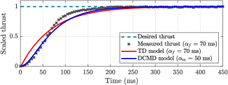
Figure 1: Step response of a rotor with a propeller. The thrust from the rotor is scaled by the maximum thrust generated from the rotor. The specifications of the rotor will be described in detail in Section VI. Note $\alpha_{f}$ and $\alpha_{m}$ are time constants of TD and DCMD models, respectively. The time constants $\alpha_{f}$ and $\alpha_{m}$ are determined experimentally.

There are several approaches to modeling the dynamics of a rotor [21, 22]. One frequently used approach is modeling the rotor angular speed as a first-order system using brushless DC-motor dynamics, which we refer to as the DCMD model [21]. The DCMD model slightly fits well with the measured thrust, as shown in Fig. 1. However, this method complicates the stability proof as rotor dynamics include squared rotor speed resulting in negative values when dealing with bidirectional rotors.

Another approach, referred to as the thrust dynamics (TD) model, simplifies the model by treating the thrust as a first-order system [22]. Satisfactory flight performance is preserved despite that the TD model is a simplified model to ease controller design. Furthermore, as shown in Fig. 1, the TD model fits the measured thrust with the acceptable mismatch. Hence, we apply the TD model and write it as follows:

$$\dot{f}_{i}=\frac{1}{\alpha_{i}}\left(f_{{cmd},i}-f_{i}\right),$$ (2)

where $f_{{cmd},i}\in\mathbb{R}$ is commanded thrust and $\alpha_{i}\in\mathbb{R^{+}}$ is the thrust time constant for the $i$-th rotor.

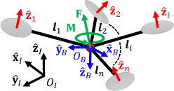
Figure 2: Coordinate frames of a general omnidirectional multirotor, where $n$ denotes the number of rotors and $\boldsymbol{l}_{i}\in\mathbb{R}^{3}$ is the position of rotor $i$ from $O_{B}$. Note that $n\geq 6$ should hold for bidirectional rotors and $n\geq 7$ for unidirectional ones.

Figure 2 shows the coordinate frame of a generalized fixed-tilt omnidirectional platform. We define the global fixed frame or the inertial frame $\mathscr{F}_{I}=O_{I},\{\hat{\mathbf{x}}_{I},\hat{\mathbf{y}}_{I},\hat{\mathbf{z}}_{I}\}$, and the body frame $\mathscr{F}_{B}=O_{B},\{\hat{\mathbf{x}}_{B},\hat{\mathbf{y}}_{B},\hat{\mathbf{z}}_{B}\}$, where $O_{B}$ is located at the center of mass (CoM) of the omnidirectional multirotor. We also define $\mathscr{F}_{i}=O_{i},\{\hat{\mathbf{x}}_{i},\hat{\mathbf{y}}_{i},\hat{\mathbf{z}}_{i}\}$ as the $i$-th rotor’s frame expressed in $\mathscr{F}_{B}$.

Under the rigid-body assumption, the Newton-Euler formulation can be written as follows:

$$\begin{split}m\dot{\mathbf{v}}&=-mg\hat{\mathbf{z}}_{I}+\mathbf{R}\mathbf{F},\\ \mathbf{J}\dot{\boldsymbol{\omega}}&=-\boldsymbol{\omega}\times\mathbf{J}\boldsymbol{\omega}+\mathbf{M},\end{split}$$ (3)

where $\mathbf{p}=[x,y,z]^{T}\in\mathbb{R}^{3}$ and $\mathbf{v}=[v_{x},v_{y},v_{z}]^{T}$ $\in\mathbb{R}^{3}$ are the position and the linear velocity of the vehicle’s CoM in the inertial frame, $\mathbf{R}\in\text{SO}(3)$ is the rotation matrix from frame $\mathscr{F}_{B}$ to $\mathscr{F}_{I}$, $m\in\mathbb{R^{+}}$ and $\mathbf{J}\in\mathbb{R}^{3\times 3}$ are the mass and inertial tensor of the platform, respectively, $\boldsymbol{\omega}=[\omega_{x},\omega_{y},\omega_{z}]^{T}\in\mathbb{R}^{3}$ is the angular velocity, and $\mathbf{F}=[F_{x},F_{y},Z_{z}]^{T}\in\mathbb{R}^{3}$ and $\mathbf{M}=[M_{x},M_{y},M_{z}]^{T}\in\mathbb{R}^{3}$ are the force and moment applied at CoM expressed in bodyframe, respectively. Note that $\dot{\mathbf{R}}=\mathbf{R}[\boldsymbol{\omega}]^{\wedge}$, where $[\cdot]^{\wedge}:\mathbb{R}^{3}\rightarrow\mathfrak{so}(3)$ is the wedge operator that maps a vector into a skew-symmetric matrix.

The relationship between the applied force $\mathbf{F}$ and moment $\mathbf{M}$ on the vehicle’s body and rotor thrusts $\{f_{i}\}^{n}_{i=1}$ can be established as follows:

$$\begin{split}\mathbf{F}=\sum_{i=1}^{n}f_{i}\hat{\mathbf{z}}_{i},\quad\mathbf{M}=\sum_{i=1}^{n}(\boldsymbol{l}_{i}\times f_{i}\hat{\mathbf{z}}_{i}+\tau_{i}\hat{\mathbf{z}}_{i}),\end{split}$$ (4)

which can be expressed in the matrix form as $[\mathbf{F},\mathbf{M}]^{T}=\textbf{A}\boldsymbol{f}$, where $\boldsymbol{f}={[f_{1},f_{2},\cdots,f_{n}]}^{T}$ and $\mathbf{A}\in{\mathbb{R}}^{6\times n}$ is the allocation matrix. Using the approximation that $\alpha_{i}\approx\alpha$, the single thrust dynamics model (2) can be expanded to collective wrench dynamics as follows:

$$\dot{\mathbf{w}}=\frac{1}{\alpha}\left(\mathbf{w}_{{cmd}}-\mathbf{w}\right),$$ (5)

where $\mathbf{w}=[\mathbf{F},\mathbf{M}]^{T}$, $\mathbf{w}_{cmd}=[\mathbf{F}_{cmd},\mathbf{M}_{cmd}]^{T}$, and $\mathbf{F}_{cmd}$ and $\mathbf{M}_{cmd}$ are the commanded force and moment, respectively, as the control inputs. With (3) and (5), the vehicle’s equation of motion with rotor dynamics can be established as follows:

$$\begin{split}m\dot{\mathbf{v}}=&{}-\alpha\mathbf{R}\dot{\mathbf{F}}-mg\hat{\mathbf{z}}_{I}+\mathbf{R}\mathbf{F}_{cmd},\end{split}$$ (6)

$$\begin{split}\mathbf{J}\dot{\boldsymbol{\omega}}=&{}-\alpha\dot{\mathbf{M}}-\boldsymbol{\omega}\times\mathbf{J}\boldsymbol{\omega}+\mathbf{M}_{cmd}.\end{split}$$ (7)

By including rotor dynamics in the Newton-Euler equation (3), $-\alpha\mathbf{R}\dot{\mathbf{F}}$ and $-\alpha\dot{\mathbf{M}}$ appear in the equation of motion, which deteriorate the tracking performance in case of slow rotor response (resulting in large $\alpha$), especially for aggressive flights. To mitigate this issue, we compensate for these undesirable values in the controller design in Section IV.

IV GEOMETRIC TRACKING CONTROL

In this section, we provide a control method for the omnidirectional multirotor to track the desired pose based on the modeling from Section III. Unlike conventional multirotor controllers [23, 24], tracking position and attitude commands are carried out in two different control loops since the translational and rotational dynamics are decoupled. We utilized a geometric PD controller, where we do not apply the integral term as it can amplify the rotor’s settling time due to its adaptive nature. Furthermore, we define force and moment errors to take rotor dynamics into account in the control design.

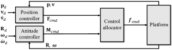
Figure 3: The control diagram of proposed controller.

Figure 3 shows the overall control diagram of the proposed controller. The inputs $\mathbf{p}_{d}=[x_{d},y_{d},z_{d}]^{T}\in\mathbb{R}^{3}$, $\mathbf{v}_{d}=[v_{x_{d}},v_{y_{d}},v_{z_{d}}]^{T}\in\mathbb{R}^{3}$, and $\dot{\mathbf{v}}_{d}$ are fed to the position controller along with the actual position $\mathbf{p}$ and velocity $\mathbf{v}$. Simultaneously, the inputs $\mathbf{R}_{d}\in\text{SO}(3)$, $\boldsymbol{\omega}_{d}=[\omega_{x_{d}},\omega_{y_{d}},\omega_{z_{d}}]^{T}\in\mathbb{R}^{3}$, and $\dot{\boldsymbol{\omega}}_{d}$ are fed to the attitude controller along with actual rotation matrix $\mathbf{R}$ and angular velocity $\boldsymbol{\omega}$. Outputs from position and attitude controllers, commanded force $\mathbf{F}_{\textrm{cmd}}$ and moment $\mathbf{M}_{\textrm{cmd}}$, are sent to the control allocator to generate $\boldsymbol{f}_{cmd}$ by $\boldsymbol{f}_{cmd}=\mathbf{A}^{-1}[\mathbf{F}_{\textrm{cmd}},\mathbf{M}_{\textrm{cmd}}]^{T}.$

For the position controller, we define position error $\mathbf{e}_{p}=[e_{x},e_{y},e_{z}]^{T}\in\mathbb{R}^{3}$, velocity error $\mathbf{e}_{v}=[e_{v_{x}},e_{v_{y}},e_{v_{z}}]^{T}\in\mathbb{R}^{3}$, and force error $\mathbf{e}_{F}\in\mathbb{R}^{3}$ by $\mathbf{e}_{p}=\mathbf{p}-\mathbf{p}_{d}$, $\mathbf{e}_{v}=\mathbf{v}-\mathbf{v}_{d}$, and $\mathbf{e}_{F}=\mathbf{F}-\mathbf{F}_{d}$, where desired force $\mathbf{F}_{d}\in\mathbb{R}^{3}$ is defined as

$$\mathbf{F}_{{d}}=\mathbf{R}^{T}\left(-{k}_{p}\mathbf{e}_{p}-{k}_{v}\mathbf{e}_{v}+mg\hat{\mathbf{z}}_{I}+m\dot{\mathbf{v}}_{d}\right),$$ (8)

for $k_{p}\in\mathbb{R^{+}}$ and $k_{v}\in\mathbb{R^{+}}$ being position and velocity gains, respectively.

To accommodate the settling time of the generated force, the force controller is designed as follows:

$$\mathbf{F}_{{cmd}}=\mathbf{F}_{{d}}+\alpha\dot{\mathbf{F}}_{{d}}.$$ (9)

For the attitude controller, we define attitude error $\mathbf{e}_{R}=$ $[e_{R_{x}},e_{R_{y}},e_{R_{z}}]^{T}$ $\in\mathbb{R}^{3}$, angular velocity error $\mathbf{e}_{\omega}=$ $[e_{\omega_{x}},e_{\omega_{y}},e_{\omega_{z}}]^{T}$ $\in\mathbb{R}^{3}$, and moment error $\mathbf{e}_{M}\in\mathbb{R}^{3}$ as $\mathbf{e}_{R}=\frac{1}{2}\left[\mathbf{R}_{d}^{T}\mathbf{R}-\mathbf{R}^{T}\mathbf{R}_{d}\right]^{\vee}$, $\mathbf{e}_{\omega}=\boldsymbol{\omega}-\mathbf{R}^{T}\mathbf{R}_{d}\boldsymbol{\omega}_{d}$, and $\mathbf{e}_{M}=\mathbf{M}-\mathbf{M}_{d},$ where the vee operator $[\cdot]^{\vee}:\mathfrak{so}(3)\rightarrow\mathbb{R}^{3}$ is the inverse of the wedge operator. The desired moment $\mathbf{M}_{{d}}\in\mathbb{R}^{3}$ is defined as

$$\mathbf{M}_{d}=-k_{R}\mathbf{e}_{R}-k_{\omega}\mathbf{e}_{\omega}+{\boldsymbol{\omega}}\times\mathbf{J}{\boldsymbol{\omega}}\\ -\mathbf{J}\left(\left[{\boldsymbol{\omega}}\right]^{\wedge}\mathbf{R}^{T}\mathbf{R}_{d}{\boldsymbol{\omega}}_{d}-\mathbf{R}^{T}\mathbf{R}_{d}\dot{{\boldsymbol{\omega}}}_{d}\right),$$ (10)

where $k_{R}\in\mathbb{R^{+}}$ and $k_{\omega}\in\mathbb{R^{+}}$ are attitude and angular velocity gains, respectively.

To resolve the settling time of the generated moment, the moment controller is designed as follows:

$$\mathbf{M}_{{cmd}}=\mathbf{M}_{{d}}+\alpha\dot{\mathbf{M}}_{{d}}.$$ (11)

For the control stability analysis, we apply the assumption that the force and the moment are decoupled. We first analyze the stability of translational and rotational systems individually and then combine the results for the overall system’s stability.

Proposition 1: (Global exponential stability of the translational system) Consider the commanded force $\mathbf{F}_{{cmd}}$ defined in (9). If positive design constants $k_{p}$, $k_{v}$, and $c_{1}$ satisfy

$$\begin{split}k_{p}>\frac{c_{1}k_{v}^{2}+2c_{1}k_{v}-c_{1}^{2}}{m\left(4\left(k_{v}-c_{1}\right)-1\right)},\quad k_{v}>c_{1}+\frac{1}{4},\end{split}$$ (12)

then the zero equilibrium of the translation tracking error dynamics of $\mathbf{e}_{p},\mathbf{e}_{v}$, and $\mathbf{e}_{F}$ is globally exponentially stable.

Proof:

Let a Lyapunov function candidate $\mathcal{V}_{1}$ for the translational system be

$$\mathcal{V}_{1}=\frac{1}{2}k_{p}\left\|\mathbf{e}_{p}\right\|^{2}+\frac{1}{2}m\left\|\mathbf{e}_{v}\right\|^{2}+\frac{1}{2}\alpha\left\|\mathbf{e}_{F}\right\|^{2}+c_{1}\mathbf{e}_{p}\cdot\mathbf{e}_{v},$$ (13)

where $\left\|\cdot\right\|$ denotes Euclidean norm.

By Cauchy-Schwartz inequality, we can show that, for $k_{p}$ satisfying (12), $\mathcal{V}_{1}$ is bounded by

$$\mathbf{z}_{1}^{T}\mathbf{M}_{11}\mathbf{z}_{1}\leq\mathcal{V}_{1}\leq\mathbf{z}_{1}^{T}\mathbf{M}_{12}\mathbf{z}_{1},$$ (14)

where $\mathbf{z}_{1}=\left[\left\|\mathbf{e}_{p}\right\|,\left\|\mathbf{e}_{v}\right\|,\left\|\mathbf{e}_{F}\right\|\right]^{T}\in\mathbb{R}^{3}$, and the matrices $\mathbf{M}_{11}\text{ and }\mathbf{M}_{12}\in\mathbb{R}^{3\times 3}$ are defined as

$$\mathbf{M}_{11}=\frac{1}{2}\begin{bmatrix}k_{p}&-c_{1}&0\\ -c_{1}&m&0\\ 0&0&\alpha\end{bmatrix},\quad\mathbf{M}_{12}=\frac{1}{2}\begin{bmatrix}k_{p}&c_{1}&0\\ c_{1}&m&0\\ 0&0&\alpha\end{bmatrix}.$$

Now we deal with the boundness of $\dot{\mathcal{V}}_{1}$. From (5) and (8)–(9), the force error dynamics can be written as

$$\alpha\dot{\mathbf{e}}_{F} =\alpha\dot{\mathbf{F}}-\alpha\dot{\mathbf{F}}_{d}=({\mathbf{F}}_{cmd}-{\mathbf{F}})-\alpha\dot{\mathbf{F}}_{d}$$ (15)

$$=-\mathbf{e}_{F}.$$

From (6), (8)–(9), and (15), the velocity error dynamics can be written as

$$m\dot{\mathbf{e}}_{v} =m\dot{\mathbf{v}}-m\dot{\mathbf{v}}_{d}=-\alpha\mathbf{R}\dot{\mathbf{F}}-mg\hat{\mathbf{z}}_{I}+\mathbf{R}\mathbf{F}_{cmd}-m\dot{\mathbf{v}}_{d}$$ (16)

$$=-k_{p}\mathbf{e}_{p}-k_{v}\mathbf{e}_{v}+\mathbf{R}\mathbf{e}_{F}.$$

Using (15)–(16), the time derivative of $\mathcal{V}_{1}$ is given by

$$\dot{\mathcal{V}}_{1}= \>k_{p}\mathbf{e}_{p}\cdot\mathbf{e}_{v}+m\mathbf{e}_{v}\cdot\dot{\mathbf{e}}_{v}+\alpha\mathbf{e}_{F}\cdot\dot{\mathbf{e}}_{F}$$ (17)

$$+c_{1}\left(\dot{\mathbf{e}}_{p}\cdot\mathbf{e}_{v}+\mathbf{e}_{p}\cdot\dot{\mathbf{e}}_{v}\right)$$

$$= -\frac{c_{1}k_{p}}{m}\left\|\mathbf{e}_{p}\right\|^{2}-\left(k_{v}-c_{1}\right)\left\|\mathbf{e}_{v}\right\|^{2}-\left\|\mathbf{e}_{F}\right\|^{2}$$

$$+\frac{c_{1}k_{v}}{m}\mathbf{e}_{p}\cdot\mathbf{e}_{v}+\mathbf{R}\mathbf{e}_{F}\cdot\left(\mathbf{e}_{v}+\frac{c_{1}}{m}\mathbf{e}_{p}\right).$$

Since $\left\|\mathbf{R}\mathbf{e}_{F}\right\|=\left\|\mathbf{e}_{F}\right\|$ holds by the property of rotation matrix [25], we can show that $\dot{\mathcal{V}}_{1}$ is bounded by

$$\dot{\mathcal{V}}_{1}\leq-\mathbf{z}_{1}^{T}\mathbf{W}_{1}\mathbf{z}_{1},$$ (18)

where

$$\mathbf{W}_{1}=\begin{bmatrix}\vspace{0.1 cm}\dfrac{c_{1}k_{p}}{m}&-\dfrac{c_{1}k_{v}}{2m}&-\dfrac{c_{1}}{2m}\\ \vspace{0.1 cm}-\dfrac{c_{1}k_{v}}{2m}&k_{v}-c_{1}&-\dfrac{1}{2}\\ -\dfrac{c_{1}}{2m}&-\dfrac{1}{2}&1\end{bmatrix}.$$

With the positive design constants $k_{p}$, $k_{v}$, and $c_{1}$ satisfying (12), the matrices $\mathbf{M}_{11},\mathbf{W}_{12},\text{and }\mathbf{W}_{1}$ are always positive definite. As a result, $\dot{\mathcal{V}}_{1}$ is always negative with the region of attraction $\mathbf{z}_{1}\in\mathbb{R}^{3}$, which implies that the translational motion of the system is globally exponentially stable in the presence of rotor dynamics. ∎

To show the stability of the rotational system, we first define the rotational error function between two rotation matrices, $\mathbf{R}_{1}$ and $\mathbf{R}_{2}$, as follows:

$$\Psi\left(\mathbf{R}_{1},\mathbf{R}_{2}\right)=\frac{1}{2}\operatorname{tr}\left(\mathbf{I}_{3}-\mathbf{R}_{2}^{T}\mathbf{R}_{1}\right),$$ (19)

where $\mathbf{I}_{3}$ is the $3\times 3$ identity matrix, $\operatorname{tr}(\cdot)$ is the trace of a square matrix. Note that $\Psi\left(\mathbf{R}_{1},\mathbf{R}_{2}\right)$ is bounded by $0\leq\Psi\left(\mathbf{R}_{1},\mathbf{R}_{2}\right)\leq 2$, and $\Psi\left(\mathbf{R}_{1},\mathbf{R}_{2}\right)=2$ if and only if the rotation angle between $\mathbf{R}_{1}$ and $\mathbf{R}_{2}$ is 180 degrees.

Proposition 2: (Almost global exponential stability of the rotational system) Consider the commanded moment $\mathbf{M}_{{cmd}}$ defined in (11). If the vehicle’s initial rotation matrix $\mathbf{R}$ satisfies

$$\Psi\left(\mathbf{R},\mathbf{R}_{d}\right)<2,$$ (20)

and positive positive design constants $k_{R}$, $k_{\omega}$, and $c_{2}$ satisfy

$$\begin{split}k_{R}>\frac{c_{2}k_{\omega}^{2}}{\lambda_{m}\left(4\left(k_{\omega}-c_{2}\right)-1\right)},\quad k_{\omega}>c_{2}+\frac{1}{4},\end{split}$$ (21)

where $\lambda_{m}$ denote the minimum eigenvalue of inertia tensor $\mathbf{J}$, then the zero equilibrium of the rotational tracking error dynamics of $\mathbf{e}_{R},\mathbf{e}_{\omega}$, and $\mathbf{e}_{M}$ is almost globally exponentially stable.

Proof:

Let a Lyapunov function candidate for rotational system $\mathcal{V}_{2}$ be

$$\mathcal{V}_{2}=\frac{1}{2}\mathbf{e}_{\omega}\cdot\mathbf{J}\mathbf{e}_{\omega}+k_{R}\Psi\left(\mathbf{R},\mathbf{R}_{d}\right)+\frac{1}{2}\alpha\left\|\mathbf{e}_{M}\right\|^{2}+c_{2}\mathbf{e}_{R}\cdot\mathbf{e}_{\omega}.$$ (22)

It can be shown that $\Psi\left(\mathbf{R},\mathbf{R}_{d}\right)$ is bounded by

$$\frac{1}{2}\left\|\mathbf{e}_{R}\right\|^{2}\leq\Psi\left(\mathbf{R},\mathbf{R}_{d}\right)\leq\frac{1}{2-\psi}\left\|\mathbf{e}_{R}\right\|^{2},$$ (23)

where $\psi\in\mathbb{R^{+}}$ satisfies $\Psi\left(\mathbf{R},\mathbf{R}_{d}\right)\leq\psi<2$ (see [26, Appendix B]). Using (23) and $\lambda_{{m}}\left\|\mathbf{e}_{\omega}\right\|^{2}\leq\mathbf{e}_{\omega}\cdot\mathbf{J}\mathbf{e}_{\omega}\leq\lambda_{{M}}\left\|\mathbf{e}_{\omega}\right\|^{2}$, where $\lambda_{M}$ is the maximum eigenvalue of $\mathbf{J}$, we can show that, for $k_{R}$ and $k_{\omega}$ satisfying (21), $\mathcal{V}_{2}$ is bounded by

$$\mathbf{z}_{2}^{T}\mathbf{M}_{21}\mathbf{z}_{2}\leq\mathcal{V}_{2}\leq\mathbf{z}_{2}^{T}\mathbf{M}_{22}\mathbf{z}_{2},$$ (24)

where $\mathbf{z}_{2}=\left[\left\|\mathbf{e}_{R}\right\|,\left\|\mathbf{e}_{\omega}\right\|,\left\|\mathbf{e}_{M}\right\|\right]^{T}\in\mathbb{R}^{3}$, and the matrices $\mathbf{M}_{21}\text{ and }\mathbf{M}_{22}\in\mathbb{R}^{3\times 3}$ are defined as

$$\mathbf{M}_{21}=\frac{1}{2}\begin{bmatrix}k_{R}&-c_{1}&0\\ -c_{2}&\lambda_{m}&0\\ 0&0&\alpha\end{bmatrix},\mathbf{M}_{22}=\frac{1}{2}\begin{bmatrix}\frac{2k_{R}}{2-\psi}&c_{2}&0\\ c_{2}&\lambda_{M}&0\\ 0&0&\alpha\end{bmatrix}.$$

Now we deal with the boundness of $\dot{\mathcal{V}}_{2}$. In [26, Appendix B], it has been shown that the following relationships hold:

$$\dot{\Psi}\left(\mathbf{R},\mathbf{R}_{d}\right)=\mathbf{e}_{R}\cdot\mathbf{e}_{\omega},\quad\left\|\dot{\mathbf{e}}_{R}\right\|\leq\left\|\mathbf{e}_{\omega}\right\|.$$ (25)

From (5) and (10)–(11), the moment error dynamics can be written as

$$\alpha\dot{\mathbf{e}_{M}} =\alpha\dot{\mathbf{M}}-\alpha\dot{\mathbf{M}_{d}}=({\mathbf{M}}_{cmd}-{\mathbf{M}})-\alpha\dot{\mathbf{M}}_{d}$$ (26)

$$=-\mathbf{e}_{M}.$$

From (7), (10)–(11), and (26), the angular velocity error dynamics can be written as

$$\mathbf{J}\dot{\mathbf{e}}_{\omega} =\mathbf{J}\dot{\boldsymbol{\omega}}-\mathbf{J}\dot{\left(\mathbf{R}^{T}\mathbf{R}_{d}\boldsymbol{\omega}_{d}\right)}$$ (27)

$$=\mathbf{J}\dot{\boldsymbol{\omega}}+\mathbf{J}\left(\left[{\boldsymbol{\omega}}\right]^{\wedge}\mathbf{R}^{T}\mathbf{R}_{d}\boldsymbol{\omega}_{d}-\mathbf{R}^{T}\mathbf{R}_{d}\dot{\boldsymbol{\omega}}_{d}\right)$$

$$=-k_{R}\mathbf{e}_{R}-k_{\omega}\mathbf{e}_{\omega}+\mathbf{e}_{M}.$$

Using (25)–(27), the time derivative of $\mathcal{V}_{2}$ is given by

$$\dot{\mathcal{V}}_{2}= \>\mathbf{e}_{\omega}\cdot\mathbf{J}\dot{\mathbf{e}}_{\omega}+k_{R}\dot{\Psi}\left(\mathbf{R},\mathbf{R}_{d}\right)+\alpha\mathbf{e}_{M}\cdot\dot{\mathbf{e}}_{M}$$ (28)

$$+c_{2}\left(\dot{\mathbf{e}}_{R}\cdot\mathbf{e}_{\omega}+\mathbf{e}_{R}\cdot\dot{\mathbf{e}}_{\omega}\right)$$

$$= -k_{\omega}\left\|\mathbf{e}_{\omega}\right\|^{2}-\left\|\mathbf{e}_{M}\right\|^{2}-c_{2}k_{R}\mathbf{e}_{R}\cdot\mathbf{J}^{-1}\mathbf{e}_{R}+c_{2}\dot{\mathbf{e}}_{R}\cdot\mathbf{e}_{\omega}$$

$$-c_{2}k_{\omega}\mathbf{e}_{R}\cdot\mathbf{J}^{-1}\mathbf{e}_{\omega}+\mathbf{e}_{M}\cdot\mathbf{e}_{\omega}+c_{2}\mathbf{e}_{R}\cdot\mathbf{J}^{-1}\mathbf{e}_{M}.$$

As $\left\|\dot{\mathbf{e}}_{R}\right\|\leq\left\|\mathbf{e}_{\omega}\right\|$, we can show that $\dot{\mathcal{V}}_{2}$ is bounded by

$$\dot{\mathcal{V}}_{2}\leq-\mathbf{z}_{2}^{T}\mathbf{W}_{2}\mathbf{z}_{2},$$ (29)

where

$$\mathbf{W}_{2}=\begin{bmatrix}\vspace{0.1 cm}\dfrac{c_{2}k_{R}}{\lambda_{m}}&\dfrac{c_{2}k_{\omega}}{2\lambda_{m}}&-\dfrac{c_{2}}{2\lambda_{M}}\\ \vspace{0.1 cm}\dfrac{c_{2}k_{\omega}}{2\lambda_{m}}&k_{\omega}-c_{2}&-\dfrac{1}{2}\\ -\dfrac{c_{2}}{2\lambda_{M}}&-\dfrac{1}{2}&1\end{bmatrix}.$$

With the positive design constants $k_{R}$, $k_{\omega}$, and $c_{2}$ satisfying (21), the matrices $\mathbf{M}_{21},\mathbf{M}_{22},\text{and }\mathbf{W}_{2}$ are always positive definite. As a result, $\dot{\mathcal{V}}_{2}$ is always negative with the region of attraction in (20), which implies that the rotational motion of the system is almost globally exponentially stable in the presence of the rotor dynamics. ∎

Theorem1: (Almost global exponential stability of complete system) Consider the commanded force $\mathbf{F}_{{cmd}}$ and the commanded moment $\mathbf{M}_{{cmd}}$ defined in (9) and (11). If positive design constants $c_{1}$, $c_{2}$, $k_{p}$, $k_{v}$, $k_{R}$, and $k_{\omega}$ satisfy (12) and (21), then the zero equilibrium of the tracking error dynamics $\mathbf{e}_{p}$, $\mathbf{e}_{v}$, $\mathbf{e}_{R}$, $\mathbf{e}_{\omega}$, $\mathbf{e}_{F}$, and $\mathbf{e}_{M}$ is exponentially stable.

Proof:

Let a Lyapunov function candidate $\mathcal{V}$ for the complete system be

$$\mathcal{V}=\mathcal{V}_{1}+\mathcal{V}_{2}.$$ (30)

Using (14) and (24), the bound of $\mathcal{V}$ can be written as

$$\mathbf{z}_{1}^{T}\mathbf{M}_{11}\mathbf{z}_{1}+\mathbf{z}_{2}^{T}\mathbf{M}_{21}\mathbf{z}_{2}\leq\mathcal{V}\leq\mathbf{z}_{1}^{T}\mathbf{M}_{12}\mathbf{z}_{1}+\mathbf{z}_{2}^{T}\mathbf{M}_{22}\mathbf{z}_{2}.$$ (31)

From (18) and (29), the time derivative of $\mathcal{V}$ is bounded by

$$\dot{\mathcal{V}}\leq-\mathbf{z}_{1}^{T}\mathbf{W}_{1}\mathbf{z}_{1}-\mathbf{z}_{2}^{T}\mathbf{W}_{2}\mathbf{z}_{2}.$$ (32)

With the positive design constants satisfying (12) and (21), the matrices $\mathbf{M}_{11}$, $\mathbf{M}_{12}$, $\mathbf{M}_{21}$, $\mathbf{M}_{22}$, $\mathbf{W}_{1}$, and $\mathbf{W}_{2}$ are always positive definite. As a result, the complete system is almost globally exponentially stable in the presence of the rotor dynamics, when the region of attraction is given by (20). ∎

V Simulation

In this section, we present the simulation results validating the proposed controller’s stability. Furthermore, we compare the proposed controller with a conventional controller for the tracking performance. The conventional controller has $\alpha_{f}=0$, i.e., the rotors are directly controlled, resulting in $\mathbf{F}_{d}$ and $\mathbf{M}_{d}$ as control inputs. For the simulated omnidirectional multirotor, we choose to utilize the configuration with six fixed-tilt bidirectional rotors proposed in [17], which is the minimal rotor configuration with omnidirectionality. We use the DCMD model for the rotor dynamics to set a realistic simulation environment. The system parameters are chosen to match the real-world platform. We use maximum thrust $f_{max}=10$ N, $m=1$ kg, $\mathbf{J}=\operatorname{diag}(0.03,0.03,0.03)$ kg$\cdot$m², $\left\|\boldsymbol{l}_{i}\right\|=0.15$ m, $\alpha_{m}=0.1$ s, ${\mu}/{\kappa}=0.15$, $k_{p}=3.0$, $k_{v}=1.0$, $k_{R}=1.0$, and $k_{\omega}=1.0$. The control gains $k_{x}$, $k_{v}$, $k_{R}$, $k_{\omega}$, and the user-designed constants $c_{1}$ and $c_{2}$ satisfy (12) and (21). We obtain the values of $\dot{\mathbf{F}}_{{d}}$ and $\dot{\mathbf{M}}_{{d}}$ using finite difference approximation.

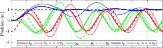
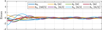
Figure 4: (T-B): The top 2 figures denote the omnidirectional multirotor’s position and errors obtained from the simulation using the proposed controller, and the last figure shows the errors obtained using a conventional controller. The subscript $p$ and $c$ in the first figure denote that the values are from the proposed and conventional controllers, respectively. Rotation and angular velocity errors along other than the $x^{I}$-axis are not shown as their values are always 0.

To demonstrate the omnidirectional flight capability, we designed the following desired trajectory: the desired position circling counterclockwise with both radius and height set to 1 m, while the desired rotation matrix rotates along the $\mathbf{x}^{I}$-axis with a constant angular speed of 1 rad/s. The initial position and rotation are set to $\mathbf{p}=[0,0,0]^{T}$ and $\mathbf{R}=\mathbf{I}_{3}$. The simulation results are shown in Fig. 4. The platform tracks the desired trajectory. For the proposed controller, the tracking errors converge to zero exponentially with minor steady-state errors. The steady-state errors are unavoidable due to the PD structure of the proposed controller. For the conventional controller, since it ignores the rotor dynamics, the errors do not converge to zero: major oscillations occur in each error term. As mentioned in Section III, these errors become larger in the case of longer rotor response time, especially for aggressive flights.

VI Experiment

To perform a real-world experiment, we built the platform in the same configuration as mentioned in Section V. The platform’s parameters are the same as the ones from the simulation except the thrust time constant $\alpha_{f}=0.07$ s. The platform consists of a Pixhawk Cube Orange [27], communication radios, six 2200KV brushless bidirectional rotors with Gemfan 513D 3-blade 3D propellers [28] and a four-cell 1500 mAh LiPo battery. The platform’s frame is custom-built using 3D-printed parts. The platform can produce 20 N thrust in any direction. The experiments are carried out using the thrust test bench, as shown in Fig. 5. The vehicle’s force is measured using a force sensor attached to the bench.

In order to demonstrate the controller’s capabilities to accommodate rotor settling time, we measure the actuated force $\mathbf{F}$ for the given desired force $\mathbf{F}_{d}$. As the test bench only can measure the force on a single axis, we test the force along $\hat{\mathbf{z}}_{B}$, denoted by $F_{z}$. For the desired force, we selected $16\operatorname{sin}({\frac{4\pi}{3}}t)$ because this is the input force when the platform keeps rotating in $\hat{\mathbf{x}}_{I}$-axis, informed from the simulation.

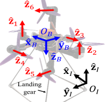
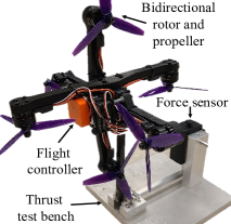
Figure 5: The coordinate frames of the omnidirectional multirotor platform using six fixed-tilt bidirectional rotors (left) and the platform attached to the thrust test bench to measure generated force on a single axis (right).

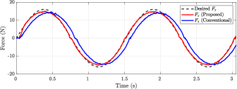
Figure 6: The time response of the generated single-axis force $F_{z}$ with the desired force. The $F_{z}$ from the proposed method (red) outperforms the one from the conventional method (blue).

The experimental results are shown in Fig. 6. The proposed method successfully accommodates the settling time, and the actuated force generated by the proposed method quickly tracks the desired value, despite minor tracking errors near the peak of the desired force. The experimental results indicate that our assumptions in the modeling and control design are sufficiently practical and can improve the control performance on a real system.

VII CONCLUSION AND FUTURE WORK

In this paper, a geometric tracking controller that uses thrust dynamics model to take rotor dynamics into account has been presented. The zero equilibrium of the tracking error dynamics is shown to be almost globally exponentially stable using the direct Lyapunov method. Additionally, the proposed controller’s stability and tracking performance are confirmed in simulations. We conduct the single-axis force experiment with the omnidirectional multirotor and confirm the viability of the proposed controller to accommodate the rotor settling time.

For future work, the DCMD model can be utilized in the analysis to characterize the rotor dynamics more accurately than the current thrust model. In addition, a real-world omnidirectional flight experiment can be performed to further demonstrate the proposed controller’s feasibility in practice.

References

- [1] H. Lee et al., “CAROS-Q: Climbing aerial robot system adopting rotor offset with a quasi-decoupling controller,” IEEE Robotics and Automation Letters, vol. 6, no. 4, pp. 8490-8497, 2021.
- [2] C. Kim, H. Lee, M. Jeong, and H. Myung, “A morphing quadrotor that can optimize morphology for transportation,” in Proc. IEEE/RSJ Int’l Conf. on Intelligent Robots and Systems (IROS), Prague, Czech Republic, 2021, pp. 9683-9689.
- [3] Z. Wu et al., “adaptive augmentation for geometric tracking control of quadrotors,” in Proc. IEEE Int’l Conf. on Robotics and Automation (ICRA), Philadelphia, PA, USA, 2022, pp. 1329-1336.
- [4] R. Mahony, V. Kumar, and P. Corke, “Multirotor aerial vehicles: Modeling, estimation, and control of quadrotor,” IEEE Robotics and Automation magazine, vol. 19, no. 3, pp. 20-32, 2012.
- [5] S. Rajappa, M. Ryll, H. H. Bülthoff, and A. Franchi, “Modeling, control and design optimization for a fully-actuated hexarotor aerial vehicle with tilted propellers,” in Proc. IEEE Int’l Conf. on Robotics and Automation (ICRA), Seattle, WA, USA, 2015, pp. 4006-4013.
- [6] A. Franchi, R. Carli, D. Bicego, and M. Ryll, “Full-pose tracking control for aerial robotic systems with laterally bounded input force,” IEEE Transactions on Robotics, vol. 34, no. 2, pp. 534-541, 2018.
- [7] P. Zheng, X. Tan, B. B. Kocer, E. Yang, and M. Kovac, “TiltDrone: A fully-actuated tilting quadrotor platform,” IEEE Robotics and Automation Letters, vol. 5, no. 4, pp. 6845-6852, 2020.
- [8] M. Ryll, H. H. Bülthoff, and P. R. Giordano, “A novel overactuated quadrotor unmanned aerial vehicle: Modeling, control, and experimental validation,” IEEE Transactions on Control Systems Technology, vol. 23, no. 2, pp. 540-556, 2015.
- [9] A. Ollero, M. Tognon, A. Suarez, D. Lee, and A. Franchi, “Past, present, and future of aerial robotic manipulators,” IEEE Transactions on Robotics, vol. 38, no. 1, pp. 626-645, 2022.
- [10] M. Tognon and A. Franchi, “Omnidirectional aerial vehicles with unidirectional thrusters: Theory, optimal design, and control,” IEEE Robotics and Automation Letters, vol. 3, no. 3, pp. 2277-2282, 2018.
- [11] M. Hamandi, K. Sawant, M. Tognon, and A. Franchi, “Omni-plus-seven (O7+): An omnidirectional aerial prototype with a minimal number of unidirectional thrusters,” in Proc. International Conference on Unmanned Aircraft Systems (ICUAS), Athens, Greece, 2020, pp. 754-761.
- [12] E. Kaufman, K. Caldwell, D. Lee, and T. Lee, “Design and development of a free-floating hexrotor UAV for 6-DOF maneuvers,” in Proc. IEEE Aerospace Conference, Big Sky, MT, USA, 2014, pp. 1-10.
- [13] M. Kamel et al., “The Voliro omniorientational hexacopter: An agile and maneuverable tiltable-rotor aerial vehicle,” IEEE Robotics and Automation Magazine, vol. 25, no. 4, pp. 34-44, 2018.
- [14] M. Allenspach et al., “Design and optimal control of a tiltrotor micro-aerial vehicle for efficient omnidirectional flight,” The International Journal of Robotics Research, vol. 39, no. 10-11, pp. 1305-1325, 2020.
- [15] S. Park, J. Her, J. Kim, and D. Lee, “Design, modeling and control of omni-directional aerial robot,” in IEEE/RSJ International Conference on Intelligent Robots and Systems (IROS), Daejeon, Korea, 2016, pp. 1570-1575.
- [16] S. Park et al., “ODAR: Aerial manipulation platform enabling omnidirectional wrench generation,” IEEE/ASME Transactions on Mechatronics, vol. 23, no. 4, pp. 1907-1918, 2018.
- [17] D. Brescianini and R. D’Andrea, “Design, modeling and control of an omni-directional aerial vehicle,” in Proc. IEEE Int’l Conf. on Robotics and Automation (ICRA), Stockholm, Sweden, 2016, pp. 3261-3266.
- [18] D. Brescianini and R. D’Andrea, “An omni-directional multirotor vehicle,” Mechatronics, vol. 55, pp. 76-93, 2018.
- [19] E. Dyer, S. Sirouspour, and M. Jafarinasab, “Energy optimal control allocation in a redundantly actuated omnidirectional UAV,” in Proc. IEEE Int’l Conf. on Robotics and Automation (ICRA), Montreal, Canada, 2019, pp. 5316-5322.
- [20] G. J. Leishman, Principles of Helicopter Aerodynamics with CD Extra. Cambridge, England: Cambridge Univ. Press, 2006.
- [21] P. Pillay and R. Krishnan, “Modeling, simulation, and analysis of permanent-magnet motor drives. II. The brushless DC motor drive,” IEEE Transactions on Industry Applications, vol. 25, no. 2, pp. 274-279, 1989.
- [22] M. Faessler, D. Falanga, and D. Scaramuzza, “Thrust mixing, saturation, and body-rate control for accurate aggressive quadrotor flight,” IEEE Robotics and Automation Letters, vol. 2, no. 2, pp. 476-482, 2017.
- [23] T. Lee, M. Leok, and N. H. McClamroch, “Geometric tracking control of a quadrotor UAV on SE(3),” in Proc. IEEE Conference on Decision and Control (CDC), Atlanta, GA, USA, 2010, pp. 5420-5425.
- [24] H. Jafarnejadsani, D. Sun, H. Lee, and N. Hovakimyan, “Optimized adaptive controller for trajectory tracking of an indoor quadrotor,” Journal of Guidance, Control, and Dynamics, vol. 40, no. 6, pp. 1415-1427, 2017.
- [25] G. Strang, Linear Algebra and Its Applications. Belmont, CA, USA: Thomson, 2006.
- [26] T. Lee, M. Leok, and N. H. McClamroch, “Control of complex maneuvers for quadrotor UAV using geometric methos on SE (3),” arXiv:1003.2005, 2010.
-
[27]
“The cube module overview.” Cube Pilot official website. https://
docs.cubepilot.org/user-guides/autopilot/the-cube-module-overview
(accessed Sep. 10, 2022). -
[28]
“Gemfan 513D-3 specifications.” Gemfan official store. https://www.
gfprops.comproducts/gemfan-513d3.html (accessed Sep. 10, 2022).