DiffTune: Auto-Tuning through Auto-Differentiation

Abstract

The performance of robots in high-level tasks depends on the quality of their lower-level controller, which requires fine-tuning. However, the intrinsically nonlinear dynamics and controllers make tuning a challenging task when it is done by hand. In this paper, we present DiffTune, a novel, gradient-based automatic tuning framework. We formulate the controller tuning as a parameter optimization problem. Our method unrolls the dynamical system and controller as a computational graph and updates the controller parameters through gradient-based optimization. The gradient is obtained using sensitivity propagation, which is the only method for gradient computation when tuning for a physical system instead of its simulated counterpart. Furthermore, we use $\mathcal{L}_{1}$ adaptive control to compensate for the uncertainties (that unavoidably exist in a physical system) such that the gradient is not biased by the unmodelled uncertainties. We validate the DiffTune on a Dubin’s car and a quadrotor in challenging simulation environments. In comparison with state-of-the-art auto-tuning methods, DiffTune achieves the best performance in a more efficient manner owing to its effective usage of the first-order information of the system. Experiments on tuning a nonlinear controller for quadrotor show promising results, where DiffTune achieves 3.5x tracking error reduction on an aggressive trajectory in only 10 trials over a 12-dimensional controller parameter space.

SUPPLEMENTARY MATERIAL

Video: https://youtu.be/g42UxcIHUdg
Code: https://github.com/Sheng-Cheng/DiffTuneOpenSource

I Introduction

Robotic systems are at the forefront of executing intricate tasks, relying on the prowess of their low-level controllers to deliver precise and agile motions. An optimal controller design starts with a meticulous analysis to ensure stability, followed by parameter tuning to achieve the intended performance on real-world robotic platforms. Traditionally, controller tuning is done either by hand using trial-and-error or proven methods for specific controllers (e.g., Ziegler–Nichols method for proportional-integral-derivative (PID) controller tuning [1]). Nevertheless, manual tuning often demands seasoned experts and is inefficient, particularly for systems with lengthy loop times or extensive parameter space.

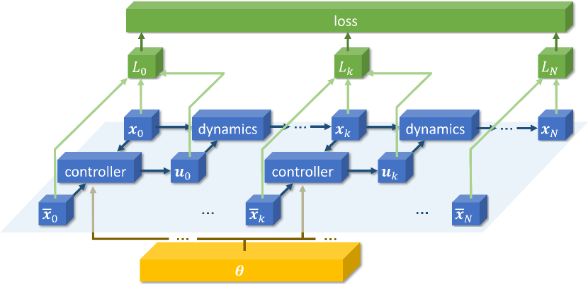
Figure 1: Illustration of an unrolled dynamical system as a computational graph.

To improve efficiency and performance, automatic tuning (or auto-tuning) methods have been investigated. Such methods integrate system knowledge, expert experience, and software tools to determine the best set of controller parameters, especially for the widely used PID controllers [2, 3, 4]. Commercial auto-tuning products have been available since 1980s [5, 3]. A desirable auto-tuning scheme should have the following three qualities: i) stability of the target system; ii) compatibility with physical systems’ data; and iii) efficiency for online deployment, possibly in real-time. However, how to design the auto-tuning scheme, simultaneously having the above three qualities, for general controllers, is still a challenge.

Existing auto-tuning methods can be categorized into model-based [6, 7] and model-free [8, 9, 10, 11, 12, 13]. Both approaches iteratively select the next set of parameters for evaluation that is likely to improve the performance over the previous trials. Model-based auto-tuning methods leverage the knowledge of the system model to improve performance, often using the gradient of the performance criterion (e.g., tracking error) and applying gradient descent so that the performance can improve based on the local gradient information [6, 7]. Stability can be ensured by explicitly leveraging knowledge about the system dynamics. However, model-based auto-tuning might not work in a real environment, where the knowledge about the dynamical model might be imperfect. This issue is especially severe when controller parameters are tuned in simulation and then deployed to a physical system.

Model-free auto-tuning methods approximate gradient or a surrogate model to improve the performance. Representative approaches include Markov chain Monte Carlo [12], Gaussian process (GP) [8, 9, 10, 11], deep neural network (DNN) [13], etc. Such approaches often make no assumptions about the model and have the advantage of compatibility with physical systems’ data owing to their data-driven nature. However, some model-free approaches, such as Bayesian optimization [14], are inefficient when tuning in high-dimensional (e.g., $>$20) parameter spaces. Besides, it is hard to establish stability guarantees with data-driven methods, where empirical methods are often applied.

To overcome the challenges in the auto-tuning scheme, we present DiffTune: an auto-tuning method based on auto-differentiation (AD). Our method is inspired by the “end-to-end” idea from the machine learning community. Specifically, in the proposed scheme, the gradient of the loss function (evaluating the performance of the controller) with respect to the controller parameters can be directly obtained and then applied to gradient descent to improve the performance. DiffTune is generally applicable to tune all the controller parameters as long as the system dynamics and controller are differentiable (we will define “differentiable” in Section III), which is the case with most of the systems. For example, algebraically computed controllers, e.g., with the structure of gain-times-error (PID [7]), are differentiable. Moreover, following the seminal work [15] that differentiates the argmin operator using the Implicit Function Theorem, one can see that controllers relying on solutions of an optimization problem to generate control actions (e.g., model predictive control (MPC) [16, 17], optimal control [18, 19], safe controllers enabled by control barrier function [20, 21, 22, 23], linear-quadratic regulator (LQR) [24]) are also differentiable.

We build DiffTune by unrolling the dynamical system into a computational graph and then applying AD to compute the gradient. Since the structure of the dynamics and controller are untouched by the unrolling operation, the system is still interpretable, which is a distinctive feature compared to the NN-structured dynamics or controllers (widely applied in reinforcement learning). Furthermore, existing tools that support AD (e.g., PyTorch [25], TensorFlow [26], JAX [27], and CasADi [28]) can be conveniently applied for gradient computation.

However, when tuning physical systems, we need gradient information based on the data collected from such systems. In this scenario, the computational graph is broken because the states of the system are obtained from sensors rather than by evaluating the dynamics function. The broken graph forbids the usage of AD over the computational graph. We present an alternative way of gradient computation, called sensitivity propagation, which is based on the sensitivity equation [29] of a dynamical system. It propagates the sensitivity of the system state to the controller parameters in the forward direction in parallel to the dynamics’ propagation. Lastly, the gradient of the loss to controller parameters is simply a weighted sum of the sensitivities. Furthermore, uncertainties and disturbances exist in physical systems. If they are not dealt with, the resulting gradient based on the nominal dynamics (free of uncertainty and disturbance) will be biased. We propose to use $\mathcal{L}_{1}$ adaptive control [30] to compensate for the uncertainties and disturbances so that the physical system behaves similarly to the nominal system. The uncertainty compensation will preserve the gradient from being biased, thus resulting in more efficient tuning.

DiffTune enjoys the three earlier mentioned qualities simultaneously: stability is inherited from the controllers with stability guarantees by design; compatibility with physical systems’ data is enabled by the sensitivity propagation; efficiency is provided since the sensitivity propagation runs forward in time and in parallel to the system’s evolution. We have validated Difftune in both simulations and experiments. DiffTune achieves smaller loss more efficiently than strong baseline auto-tuning methods AutoTune [12] and SafeOpt [9] (and its variant [31]) in simulations. Notably, in experiments, Difftune achieves a 3.5x reduction in tracking error in only 10 trials when tuning a nonlinear controller (12-dimensional parameter space) of a quadrotor for tracking an aggressive trajectory, demonstrating the efficacy of the proposed approach.

Our contributions are summarized as follows: i) We propose an auto-tuning method for controller parameters over nonlinear dynamical systems and controllers in general forms by formulating the tuning problem as a parameter optimization problem. Only differentiability of the dynamics, controller, and loss function (for tuning) is required. ii) We treat the unrolled system as a computational graph, over which we use auto-differentiation to compute the gradient efficiently. Specifically, we propose sensitivity propagation, which is compatible with data collected from a physical system and can be efficiently computed online. iii) We combine tuning with the $\mathcal{L}_{1}$ adaptive control to compensate for the model uncertainties in a physical system that can bias the computed gradient for tuning. iv) We validate the proposed approach in extensive simulations and experiments, where the compatibility with physical data, stability, and efficiency of DiffTune are demonstrated.

The remainder of the paper is organized as follows: Sections II and III review related work and background, respectively, of this paper. Section IV describes our auto-tuning method and sensitivity propagation. We also discuss uncertainty handling when using physical systems’ data. Section V shows the simulation results on a Dubins’ car and on a quadrotor. Section VI demonstrates the experimental results on a quadrotor. Finally, Section VII concludes the paper.

II Related Work

Our approach closely relates to classical work on automatic parameter tuning and recent learning-based controllers. In this section, we briefly review previous work in the following directions.

Model-based auto-tuning leverages model knowledge to infer the parameter choice for performance improvement. In [6], an auto-tuning method is proposed for LQR. The gradient of a loss function with respect to the parameterized quadratic matrix coefficients is approximated using Simultaneous Perturbation Stochastic Approximation [32], which essentially computes the difference quotients at two random perturbation directions of the current parameter values. Simulations and experiments on an inverted pendulum platform demonstrate the effectiveness of this method. The authors of [7] applied autodifferentiation to tune a PID controller with input saturation, which is done by differentiating through the model and the feedback loop. Numerical examples are provided to show the efficacy of the proposed method on single-input-single-output systems. The authors of [33] propose a probabilistic policy search method to efficiently tune a Model Predictive Contouring Control (MPCC) for quadrotor agile flight. The MPCC allows trade-offs between progress maximization and path following in real time, albeit the dimension of parameters grows linearly to the number of gates on a race track. The search of the parameters is turned into maximizing a weighted likelihood function. The approach is validated in real-world scenarios, demonstrating superior performance compared to both manually tuned controllers and state-of-the-art auto-tuning baselines in aggressive quadrotor racing. In [34], actor-critic reinforcement learning (RL) is used to tune the parameters of a differentiable MPC for agile quadrotor tracking. The proposed approach enables short-term predictions and optimization of actions based on system dynamics while retaining the end-to-end training benefits and exploratory behavior of an RL agent. Zero-shot transfer to a real quadrotor is demonstrated on different high-level tasks.

Model-free auto-tuning relies on a zeroth-order approximate gradient or surrogate performance model to decide the new candidate parameters. In [35], the authors use extremum seeking to sinusoidally perturb the PID gains and then estimate the gradient. Gradient-free methods, e.g., Metropolis-Hastings (M-H) algorithm [36], have also been used for tuning. The M-H algorithm can produce a sequence of random samples from a desired distribution that cannot be directly accessed, whereas a score function is used instead to guide the sampling. In [12], the M-H algorithm is tailored to tuning the tracking MPC controller for high-speed quadrotor racing that demands minimum-time trajectory completion. In terms of surrogate models, machine learning tools have been frequently used for their advantages in incorporating data, which, in general, make no assumptions about the systems that produce the data. In [37], an end-to-end, data-driven hyperparameter tuning is applied to an MPC using a surrogate dynamical model. Such a method jointly optimizes the hyperparameters of system identification, task specification, and control synthesis. Simulation validation is conducted in the OpenAI Gym [38] environment.

Gaussian Process is often used as a non-parametric model that approximates an unknown function from input-output pairs with probabilistic confidence measures. This property makes GP a suitable surrogate model that approximates the performance function with respect to the tuned parameters. In [8], GP is applied to approximate the unknown cost function using noisy evaluations and then induce the probability distribution of the parameters that minimize the loss. The distribution is used to determine new parameters that can maximize the relative entropy, yielding information-efficient exploration of the parameter space. The proposed method is demonstrated to tune an LQR for balancing an inverted pole using a robot arm. In [9], the authors apply Bayesian optimization [39] to controller tuning (SafeOpt), which uses GP to approximate the cost map over controller parameters while constructing safe sets of parameters to ensure safe exploration. Safe sets of parameters are constructed while exploring new parameters such that the next evaluation point that can improve the current performance will also be safe. Quadrotor experiments are presented where the proposed method is used to tune a PD position controller on a single axis. Follow-up experiments [40] demonstrate the proposed auto-tuning scheme to quadrotor control with nonlinear tracking controllers. However, one drawback of SafeOpt is that the search for the maximizer requires discretizing the parameters space, which scales poorly to the dimension of parameters. An improved version [31] applies particle swarm heuristics to perform adaptive discretization, which drastically reduces the computation time of SafeOpt to determine the maximizer. Bayesian optimization has also been applied to gait optimization for bipedal walking, where GP is used to approximate the cost map of parameterized gaits [10, 11].

Learning for control is a recently trending research direction that strives to combine the advantages of model-driven control and data-driven learning for the safe operation of a robotic system. Exemplary approaches include, but not limited to, the following: reinforcement learning [41, 42], whose goal is to find an optimal policy while gathering data and knowledge of the system dynamics from interactions with the system; imitation learning [43], which aims to mimic the actions taken by a superior controller while making decisions using less information of the system than the superior controller; and iterative learning control [44, 45], which constructs the present control action by exploiting every possibility to incorporate past control and system information, typically for systems working in a repetitive mode. A recent survey [46] provides a thorough review of the safety aspect of learning for control in robotics.

Autodifferentiation is a technique that evaluates the partial derivative of a function specified by a computer program [47, 48]. Utilizing the inherent nature of computer programs, regardless of their complexity, autodifferentiation capitalizes on the execution of elementary arithmetic operations (such as addition, subtraction, multiplication, division, etc.) and elementary functions (such as exp, log, sin, cos, etc.). By iteratively applying the chain rule to these operations, it automatically computes partial derivatives of any desired order with high accuracy while incurring only a marginal increase in the number of arithmetic operations compared to the original program. Autodifferentiation has a significant advantage over other differentiation methods, e.g., manual differentiation (prone to errors and time-consuming), numerical differentiation like finite difference (poor scalability to high-dimensional inputs and proneness to round-off errors), or symbolic differentiation (suffering from overly complicated symbolic representations of the derivative, known as “expression swell”). A comprehensive comparison of these differentiation methods is provided in [48]. There are two modes of AD, reverse mode and forward mode, both relying on the chain rule to propagate the derivative. The reverse-mode AD requires a forward pass of the computational graph and keeps the values of the intermediate nodes in the memory. Subsequently, a backward pass propagates the partial derivatives from the output to the input of the graph. The forward-mode AD propagates the partial derivatives while conducting the forward pass on the graph, storing both the values and partial derivatives of the intermediate nodes in the memory.

III Problem Formulation

Consider a discrete-time dynamical system

$$\bm{x}_{k+1}=f(\bm{x}_{k},\bm{u}_{k}),$$ (1)

where $\bm{x}_{k}\in\mathbb{R}^{n}$ and $\bm{u}_{k}\in\mathbb{R}^{m}$ are the state and control, respectively, and the initial state $\bm{x}_{0}$ is known. The control is generated by a feedback controller that tracks a desired state $\bar{\bm{x}}_{k}\in\mathbb{R}^{n}$ such that

$$\bm{u}_{k}=h(\bm{x}_{k},\bar{\bm{x}}_{k},\bm{\theta}),$$ (2)

where $\bm{\theta}\in\mathbb{R}^{p}$ denotes the parameters of the controller, e.g., $\bm{\theta}\in\mathbb{R}^{2}$ may represent the P- and D-gain in a PD controller. We assume that the state $\bm{x}_{k}$ can be measured directly or, if not, an appropriate state estimator is used. Furthermore, we assume the dynamics (1) and controller (2) are differentiable, i.e., the Jacobians $\nabla_{\bm{x}}f$, $\nabla_{\bm{u}}f$, $\nabla_{\bm{x}}h$, and $\nabla_{\bm{\theta}}h$ exist, which widely applies to general systems.

The tuning task adjusts $\bm{\theta}$ to minimize an evaluation criterion, denoted by $L(\cdot)$, which is a differentiable function of the desired states $\bar{\bm{x}}$, actual states $\bm{x}$, and control actions $\bm{u}$ over a time interval of length $N$. An illustrative example is the tracking error plus control-effort penalty, where $L(\bm{x}_{0:N},\bar{\bm{x}}_{0:N},\bm{u}_{0:N-1};\bm{\theta})=\sum_{k=0}^{N}\lVert\bm{x}_{k}-\bar{\bm{x}}_{k}\rVert^{2}+\sum_{k=0}^{N-1}\lambda\lVert\bm{u}_{k}\rVert^{2}$ with $\lambda>0$ being the penalty coefficient. We will use the short-hand notation $L(\bm{\theta})$ for conciseness in the rest of the paper.

With the setup introduced above, controller tuning can be formulated as a parameter optimization problem as follows:

$$\underset{\bm{\theta}\in\Theta}{\text{minimize}} L(\bm{\theta})$$ (P)

subject to $$\bm{x}_{k+1}=f(\bm{x}_{k},\bm{u}_{k}),$$

$$\bm{u}_{k}=h(\bm{x}_{k},\bar{\bm{x}}_{k},\bm{\theta}),$$

$$k\in\{0,1,\dots,N-1\}.$$

Note that problem (P) searches for controller parameter $\bm{\theta}$ to minimize the loss $L$ subject to the system’s dynamics and a chosen controller (to be tuned). Problem (P) is generally nonconvex due to the nonlinearity in dynamics $f$ and controller $h$. We will introduce our method, DiffTune, in Section IV for auto-tuning, especially for tuning a controller for a physical system.

IV Method

We use a gradient-based method to solve problem (P) due to its nonconvexity, where the system performance is gradually improved by adjusting the controller parameters using gradient descent. We unroll the dynamical system (1) and controller (2) into a computational graph. Figure 1 illustrates the unrolled system, which stacks the iterative procedure of state update via the “dynamics” and control-action generation via the “controller.” The gradient $\nabla_{\bm{\theta}}L$ is then applied to update the parameters $\bm{\theta}$. Specifically, since the parameters are usually confined to a feasible set $\Theta$, we use the projected gradient descent [49] to update $\bm{\theta}$:

$$\bm{\theta}\leftarrow\mathcal{P}_{\Theta}(\bm{\theta}-\alpha\nabla_{\bm{\theta}}L),$$ (3)

where $\mathcal{P}_{\Theta}$ is the projection operator that projects its operand into the set $\Theta$, and $\alpha$ is the learning rate. The feasible set $\Theta$ is used here to ensure the stability of the system, where $\Theta$ can be determined via the Lyapunov analysis or empirically determined by engineering practice.

What remains to be done is to compute the gradient $\nabla_{\bm{\theta}}L$, for which AD can be used when the computational graph is complete (e.g., in simulations). AD can be conveniently implemented using off-the-shelf tools like PyTorch [25], TensorFlow [26], JAX [27], or CasADi [28]: one will program the computational graph using the dynamics and controller and set the parameter $\bm{\theta}$ with respect to which the loss function will be differentiated.

However, AD methods cannot incorporate data (state and control) from a physical system because AD relies on a complete computation graph, whereas the computational graph corresponding to a physical system is broken. Specifically, the dynamics (1) have to be evaluated each time to obtain a new state, which is not the case in a physical system: the states are obtained through sensor measurements or state estimation rather than evaluating the dynamics (see the comparison in Figs. 2(a) and 2(b)). This explains why the computational graph is broken when considered for a physical system. Thus, AD can only be applied to auto-tuning in simulations, forbidding its usage with physical systems’ data. We introduce sensitivity propagation next to address the compatibility with physical systems’ data.

IV-A Sensitivity propagation

We first break down the gradient $\nabla_{\bm{\theta}}L$ using chain rule:

$$\nabla_{\bm{\theta}}L=\sum_{k=1}^{N}\frac{\partial L}{\partial\bm{x}_{k}}\frac{\partial\bm{x}_{k}}{\partial\bm{\theta}}+\sum_{k=0}^{N-1}\frac{\partial L}{\partial\bm{u}_{k}}\frac{\partial\bm{u}_{k}}{\partial\bm{\theta}}.$$ (4)

Since $\partial L/\partial\bm{x}_{k}$ and $\partial L/\partial\bm{u}_{k}$ can be determined once $L$ is chosen, what remains to be done is to obtain $\partial\bm{x}_{k}/\partial\bm{\theta}$ and $\partial\bm{u}_{k}/\partial\bm{\theta}$. Given that the system states $\bm{x}_{k}$ are iteratively defined using the dynamics (1), we can derive an iterative formula for $\partial\bm{x}_{k}/\partial\bm{\theta}$ and $\partial\bm{u}_{k}/\partial\bm{\theta}$ by taking partial derivative with respect to $\bm{\theta}$ on both sides of the dynamics (1) and controller (2):

$$\frac{\partial\bm{x}_{k+1}}{\partial\bm{\theta}}= (\nabla_{\bm{x}_{k}}f+\nabla_{\bm{u}_{k}}f\nabla_{\bm{x}_{k}}h)\frac{\partial\bm{x}_{k}}{\partial\bm{\theta}}+\nabla_{\bm{u}_{k}}f\nabla_{\bm{\theta}}h,$$ (5a)

$$\frac{\partial\bm{u}_{k}}{\partial\bm{\theta}}= \nabla_{\bm{x}_{k}}h\frac{\partial\bm{x}_{k}}{\partial\bm{\theta}}+\nabla_{\bm{\theta}}h,$$ (5b)

with $\partial\bm{x}_{0}/\partial\bm{\theta}=0$. Note that (5a) is essentially the sensitivity equation of a system [29, Chapter 3.3]. We name the Jacobians $\partial\bm{x}_{k}/\partial\bm{\theta}$ and $\partial\bm{u}_{k}/\partial\bm{\theta}$ by sensitivity states.

The sensitivity propagation (5a) works by propagating the sensitivity state $\partial\bm{x}_{k}/\partial\bm{\theta}$ forward in time. In fact, (5a) is a time-varying linear system with the sensitivity state $\partial\bm{x}_{k}/\partial\bm{\theta}$. The system matrix $\nabla_{\bm{x}_{k}}f+\nabla_{\bm{u}_{k}}f\nabla_{\bm{x}_{k}}h$ and the excitation $\nabla_{\bm{u}_{k}}f\nabla_{\bm{\theta}}h$ are computed each time with the data sampled from the physical system. Specifically, the coefficients $\nabla_{\bm{x}_{k}}f$, $\nabla_{\bm{u}_{k}}f$, $\nabla_{\bm{x}_{k}}h$, and $\nabla_{\bm{\theta}}h$, whose formula are known since $f$ and $h$ are known, are evaluated at sampled state $\bm{x}_{k}$ and control $\bm{u}_{k}$. Once $\{\partial\bm{x}_{k}/\partial\bm{\theta}\}_{k=0:N}$ and $\{\partial\bm{u}_{k}/\partial\bm{\theta}\}_{k=0:N-1}$ are all computed, $\nabla_{\bm{\theta}}L$ can be computed as the weighted sum of the sensitivity states, where the weights $\{\partial L/\partial\bm{x}_{k}\}_{k=0:N}$ and $\{\partial L/\partial\bm{u}_{k}\}_{k=0:N-1}$ (whose formula are also known) are evaluated at the sampled data. An illustration of how sensitivity propagation works is shown in Fig. 2(c). Furthermore, sensitivity propagation permits online tuning. Since the formulas of $\nabla_{\bm{x}_{k}}f$, $\nabla_{\bm{u}_{k}}f$, $\nabla_{\bm{x}_{k}}h$, and $\nabla_{\bm{\theta}}h$ can be derived offline, the sensitivity propagation can update $\partial\bm{x}_{k+1}/\partial\bm{\theta}$ online whenever the system data $\bm{x}_{k}$ and $\bm{u}_{k}$ are sampled. Owing to the forward-in-time nature of sensitivity propagation, the horizon $N$ can be adjusted online by need, which further contributes to the flexibility of gradient computation to a varying horizon using sensitivity propagation. We summarize the DiffTune algorithm with sensitivity propagation in Alg. 1.

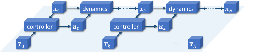
(a)

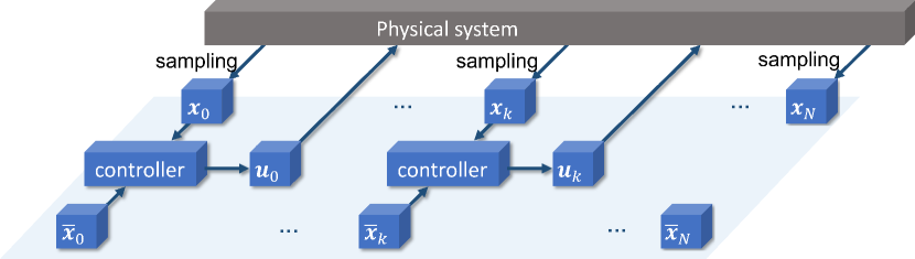
(b)

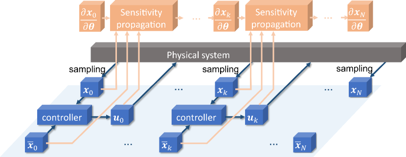
(c)

Figure 2: Difference between a conceptual dynamical system (a) and a physical system (b). Since a physical system in (b) does not have a complete computational graph for autodifferentiation, sensitivity propagation is used for gradient computation and is illustrated in (c).

Remark 1

The sensitivity propagation and forward-mode AD share the same formula as in (4) and (5). The difference lies in what type of data is applied. Two types of data are considered: The first type is from simulation, where $\bm{x}_{k}$ is obtained by the computation $\bm{x}_{k}=f(\bm{x}_{k-1},\bm{u}_{k-1})$; the second type is sampled from a physical system, where $\bm{x}_{k}$ is obtained by either sensor measurements or state estimation, which cannot be represented as the evaluation a mathematical expression. In principle, forward-mode AD can only work with data of the first type, which limits its application to auto-tuning in simulations only. Sensitivity propagation, however, can work with both types of data. The most significant usage is associated with the second-type data, which provides a straightforward method of tuning a physical system. When applied to the first type of data, the sensitivity propagation is equivalent to the forward-mode AD.

Remark 2

One may notice that the sensitivity state $\partial\bm{x}_{0}/\partial\bm{\theta}$ is set to a zero matrix. This initialization relates to how the sensitivity state is interpreted. Suppose we have sampled the sequence of state $\{\bm{x}_{k}\}_{k=0:N}$ and control $\{\bm{u}_{k}\}_{k=0:N-1}$ subject to a certain parameter $\bm{\theta}$. Consider a small perturbation $\bm{\epsilon}\in\mathbb{R}^{p}$ to $\bm{\theta}$. The sensitivity states allow inferring about the state and control sequence subject to the parameter being $\bm{\theta}+\bm{\epsilon}$ using first-order approximation (without implementing the controller with the parameter $\bm{\theta}+\bm{\epsilon}$ and then sampling the data). Specifically, we have

$$\bm{x}_{k}(\bm{\theta}+\bm{\epsilon})\approx \ \bm{x}_{k}(\bm{\theta})+\frac{\partial\bm{x}_{k}}{\partial\bm{\theta}}\bm{\epsilon},$$ (6)

$$\bm{u}_{k}(\bm{\theta}+\bm{\epsilon})\approx \ \bm{u}_{k}(\bm{\theta})+\frac{\partial\bm{u}_{k}}{\partial\bm{\theta}}\bm{\epsilon}.$$ (7)

The sensitivity state $\partial\bm{x}_{k}/\partial\bm{\theta}$ is initialized at zero such that $\bm{x}_{0}(\bm{\theta}+\bm{\epsilon})=\bm{x}_{0}(\bm{\theta})$ to ensure the same initial state despite parameter change. Therefore, how the state $\bm{x}_{k}(\bm{\theta}+\bm{\epsilon})$ will change subject to the $\bm{\epsilon}$ parameter perturbation can be inferred from the sensitivity $\partial\bm{x}_{k}/\partial\bm{\theta}$ which simply evolves with the sensitivity equation. Furthermore, the sensitivity states allow for auto-tuning without hyperparameters (e.g., learning rate $\alpha$), which is detailed in [50].

Remark 3

Although AD cannot be applied to the entire computational graph when using data from a physical system, it can still be applied to obtain the Jacobians $\nabla_{\bm{x}_{k}}f$, $\nabla_{\bm{u}_{k}}f$, $\nabla_{\bm{x}_{k}}h$, and $\nabla_{\bm{\theta}}h$. Since the iterative structure in (5) remains the same among iterations, AD packages like PyTorch [25], TensorFlow [26], JAX [27], and CasADi [28] can be applied for evaluating these Jacobians.

Algorithm 1 DiffTune

0:  Initial state $\tilde{\bm{x}}_{0}$, initial parameter $\bm{\theta}_{0}$, feasible set $\Theta$, horizon $N$, desired state $\{\bar{\bm{x}}_{k}\}_{k=0:N}$, step size $\alpha$, formulas of the Jacobians $\{\nabla_{\bm{x}}f,\nabla_{\bm{u}}f,\nabla_{\bm{x}}h,\nabla_{\bm{\theta}}h\}$, and termination condition $\mathcal{C}$.

0:  Tuned parameter $\bm{\theta}^{*}$

1:  Initialize $\bm{\theta}\leftarrow\bm{\theta}_{0}$.

2:  while $\mathcal{C}$ is FALSE do

3:     Set $\bm{x}_{0}\leftarrow\tilde{\bm{x}}_{0}$ and $\partial\bm{x}_{0}/\partial\bm{\theta}\leftarrow 0$.

4:     for $k\leftarrow 0$ to $N$ do

5:        Obtain $\bm{x}_{k}$ from system and compute $\bm{u}_{k}$ using (2).

6:        Update $\partial\bm{x}_{k+1}/\partial\bm{\theta}$ and $\partial\bm{u}_{k}/\partial\bm{\theta}$ using (5).

7:        Compute $\partial L/\partial{\bm{x}_{k}}$ and $\partial L/\partial{\bm{u}_{k}}$.

8:        Store $\partial\bm{x}_{k+1}/\partial\bm{\theta}$, $\partial\bm{u}_{k}/\partial\bm{\theta}$, $\partial L/\partial{\bm{x}_{k}}$ and $\partial L/\partial{\bm{u}_{k}}$ in memory.

9:     end for

10:     Compute $\nabla_{\bm{\theta}}L$ using (4) and update $\bm{\theta}$ by (3).

11:  end while

12:  return  the tuned parameter $\bm{\theta}^{*}\leftarrow\bm{\theta}$.

The unique aspect of sensitivity propagation is its compatibility with data from a physical system. Using such data for tuning is vital because the ultimate goal is to improve the performance of a physical system instead of its simulated counterpart. Despite the fidelity of the model in simulation, the physical system will have discrepancies with the model, leading to sub-optimal performance if the parameters come from simulation-based tuning. This phenomenon is part of the sim-to-real gap, which leads to degraded performance on physical systems compared to their simulated counterparts. The sensitivity propagation, unlike the forward- or reverse-mode AD, can still be applied to compute the gradient while using data collected from the physical system.

IV-B Auto-tuning with data from physical systems

The core of DiffTune is to obtain $\nabla_{\bm{\theta}}L$ from physical systems’ data and then apply projected gradient descent.

However, model uncertainties and noise have to be carefully handled when using such data. Controller design usually uses the nominal model of the system, which is uncertainty- and noise-free. However, both uncertainties and noise exist in a physical system. If not dealt with, then the uncertainties and noise will contaminate the sensitivity propagation, leading to biased sensitivities and, thus, biased gradient $\nabla_{\bm{\theta}}L$, which results in inefficient parameter update. Since noise can be efficiently addressed by filtering or state estimation, our focus will be on handling the model uncertainties.

Existing methods that can compensate for the uncertainties can be applied to mitigate this issue. For example, the $\mathcal{L}_{1}$ adaptive control ($\mathcal{L}_{1}$AC) is a robust adaptive control architecture that has the advantage of decoupling estimation from control, thereby allowing for arbitrarily fast adaptation subject only to hardware limitations [30]. It can be augmented to the controller to be tuned such that the resulting system, even though suffering from model uncertainties, behaves like a nominal system by $\mathcal{L}_{1}$AC’s compensation for the uncertainties. To proceed with the illustration of how $\mathcal{L}_{1}$AC works, we use continuous-time dynamics to stay consistent with the notation in the majority of the $\mathcal{L}_{1}$AC references [30, 51]. Consider the nominal system dynamics:

$${\dot{\bm{x}}^{\star}}(t)=f({\bm{x}^{\star}}(t),t)+B_{\text{m}}({\bm{x}^{\star}}(t),t)\bm{u}({\bm{x}^{\star}}(t)),\ \bm{x}^{\star}(0)=\bm{x}_{0},$$ (8)

where we use $\bm{x}^{\star}$ to denote the nominal state, $B_{\text{m}}\in\mathbb{R}^{n\times m}$ to denote the control input matrix and $\bm{u}$ to denote the control input to the system. For example, in the tuning setup, $\bm{u}$ is chosen as the baseline control $\bm{u}_{h}$ from the to-be-tuned controller $h$ in (2).

Consider the system in the presence of uncertainties:

$$\dot{\bm{x}}(t)=f(\bm{x}(t),t)+B_{\text{m}}(\bm{x}(t),t)\left(\bm{u}(\bm{x}(t))+\bm{\sigma}_{\text{m}}(\bm{x}(t),t)\right)\\ +B_{\text{um}}\bm{\sigma}_{\text{um}}(\bm{x}(t),t),$$ (9)

where $\bm{\sigma}_{\text{m}}\in\mathbb{R}^{m}$ and $\bm{\sigma}_{\text{um}}\in\mathbb{R}^{n-m}$ denote the matched and unmatched uncertainties, respectively, and $\bm{x}(0)=\bm{x}_{0}$. The matrix $B_{\text{um}}\in\mathbb{R}^{n\times(n-m)}$ satisfies $B_{\text{m}}^{\top}B_{\text{um}}=0$ and $\text{rank}([B_{\text{m}}\ B_{\text{um}}])=n$. The uncertainty $\bm{\sigma}$, defined as $\bm{\sigma}^{\top}:=[\bm{\sigma}_{\text{m}}^{\top}\ \bm{\sigma}_{\text{um}}^{\top}]$, poses challenges to the sensitivity propagation because the mapping $\bm{x}(t)\mapsto\bm{\sigma}(\bm{x}(t),t)$ may not be explicitly known, leaving $\partial\bm{\sigma}/\partial\bm{x}$ uncomputable in the sensitivity propagation. We consider the following control design $\bm{u}=\bm{u}_{\text{h}}+\bm{u}_{\text{ad}}$, with $\bm{u}_{\text{ad}}$ being the adaptive control, which results in the following system:

$$\dot{\bm{x}}(t)=f(\bm{x}(t),t)+B_{\text{um}}(\bm{x}(t),t)\bm{\sigma}_{\text{um}}(\bm{x}(t),t)\\ +B_{\text{m}}(\bm{x}(t),t)(\bm{u}_{h}(\bm{x}(t))+\bm{u}_{\text{ad}}(t)+\bm{\sigma}_{\text{m}}(\bm{x}(t),t)).$$ (10)

The adaptive control $\bm{u}_{\text{ad}}$ aims to cancel out the matched uncertainty $\bm{\sigma}_{\text{m}}$, i.e., $\lVert\bm{\sigma}_{\text{m}}+\bm{u}_{\text{ad}}\rVert\approx 0$ (see [30, 52, 53, 54] for details of how $\mathcal{L}_{1}$AC is implemented). Specifically, $\mathcal{L}_{1}$AC estimates the uncertainty $\bm{\sigma}$ based on a state predictor and adaptation law. The state predictor propagates the state prediction $\hat{\bm{x}}$ based on the estimated uncertainty $\hat{\bm{\sigma}}$ and control inputs $\bm{u}_{h}$ and $\bm{u}_{\text{ad}}$, i.e.,

$$\dot{\hat{\bm{x}}}(t)=f(\bm{x}(t),t)+B_{\text{um}}(\bm{x}(t),t)\hat{\bm{\sigma}}_{\text{um}}(t)+A_{s}(\hat{\bm{x}}(t)-{\bm{x}}(t))\\ +B_{\text{m}}(\bm{x}(t),t)\left(\bm{u}_{h}(\bm{x}(t))+\hat{\bm{\sigma}}_{\text{m}}(t)+\bm{u}_{\text{ad}}(t)\right),$$ (11)

where $A_{s}\in\mathbb{R}^{n\times n}$ is a Hurwitz matrix, and $\hat{\bm{x}}(0)=\bm{x}_{0}$. The error $\hat{\bm{x}}(t)-\bm{x}(t)$ between the predicted and actual states are used to compute the estimated uncertainty, where we use the piecewise-constant adaptation law [30]:

$$\hat{\bm{\sigma}}(t)=\left[\begin{smallmatrix}\hat{\bm{\sigma}}_{\text{m}}(t)\\ \hat{\bm{\sigma}}_{\text{um}}(t)\end{smallmatrix}\right]=-[B_{\text{m}}\ B_{\text{um}}]^{-1}\text{expm}(A_{s}T_{s}-I)^{-1}\\ A_{s}\text{expm}(A_{s}T_{s})(\hat{\bm{x}}(t)-\bm{x}(t)),$$ (12)

with $T_{s}$ being the sample time of $\mathcal{L}_{1}$AC, expm$(\cdot)$ denoting matrix exponential, and $I$ being the identity matrix. The uncertainty’s estimation error $\lVert\bm{\sigma}-\hat{\bm{\sigma}}\rVert$ is shown to be uniformly bounded under a set of mild regularity assumptions [55, 56]. Once the estimated uncertainty $\hat{\bm{\sigma}}$ is computed, the compensation $\bm{u}_{\text{ad}}$ is obtained by low-pass filtering $\hat{\bm{\sigma}}$, i.e.,

$$\bm{u}_{\text{ad}}(s)=C(s)\hat{\bm{\sigma}}_{\text{m}}(s),$$ (13)

with $s$ being the complex variable in the frequency domain, and $C(s)$ is the transfer function of the low-pass filter (LPF). The LPF is used here because the compensation is limited by the bandwidth of the actuator, where only the low-frequency components of $\hat{\bm{\sigma}}$ can be implemented by the actuator. It can be shown that the residual $\lVert\bm{\sigma}_{\text{m}}+\bm{u}_{\text{ad}}\rVert$ is bounded [51, 57], and the error norm $\lVert{\bm{x}^{\star}}-\bm{x}\rVert$ between the nominal state ${\bm{x}^{\star}}$ and the closed-loop state $\bm{x}$ in (10) is uniformly bounded both in transient and steady-state [56, 57], which renders the uncertain system (10) behaving similar to the nominal system (8). Therefore, the sensitivity propagation remains unchanged while $\mathcal{L}_{1}$AC handles the uncertainties. We will illustrate how the $\mathcal{L}_{1}$AC facilitates the auto-tuning of a physical system in Sections V and VI.

Remark 4

Note that $\bm{u}_{\text{ad}}$ is not applied to the sensitivity propagation (only $\bm{u}_{h}$ is applied) because $\bm{u}_{\text{ad}}$ is used to cancel out the uncertainty $\bm{\sigma}_{\text{m}}$ to preserve the validity of the nominal dynamics (8).

IV-C Open-source DiffTune toolset

Our toolset DiffTuneOpenSource [58] is publicly available, which facilitates users’ DiffTune applications in two ways. First, it enables the automatic generation of the partial derivatives required in sensitivity propagation. In this way, a user only needs to program the dynamics and controller, eliminating the need for additional programming of the partial derivatives. Second, we provide a template that allows users to quickly set up DiffTune for custom systems and controllers. The Dubin’s car and quadrotor cases used in Section V are used as examples to illustrate the usage of the template.

V Simulation results

In this section, we implement DiffTune for a Dubin’s car and a quadrotor in simulations, where the controller in each case is differentiable. For all simulations, we use ode45 to obtain the system states by integrating the continuous-time dynamics (mimicking the continuous-time process on a physical system). The states are sampled at discrete-time steps. We use the sensitivity propagation to compute $\nabla_{\bm{\theta}}L$, where the discrete-time dynamics in (1) are obtained by forward-Euler discretization.

We intend to answer the following questions through the simulation study: 1. How does DiffTune compare to other auto-tuning methods? Since equipment wear is not an issue for tuning in simulations, we conduct sufficiently many trials to understand the asymptotic performance of auto-tuning methods for comparison. 2. How can the tuned parameters generalize to other unseen trajectories during tuning? 3. How does $\mathcal{L}_{1}$AC help tuning when the system has uncertainties? We show our results in the following subsections while supplying the details of modeling and tuning configurations in Appendices A and B.

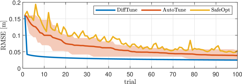
Figure 3: Comparison of auto-tuning of Dubin’s car using DiffTune (with learning rate $\alpha=1$), AutoTune [12] and SafeOpt [9]. The shaded area shows the range of RMSEs (min to max) achieved in a total of 10 runs of AutoTune.

V-A Dubin’s car

Comparison to other methods: We compare DiffTune with strong baseline auto-tuning methods: AutoTune [12] and SafeOpt [9]. We compare the tuning performance on a circular trajectory and assign 100 trials in each method. Other details of implementation are available in Appendix A. The results are shown in Fig. 3. It is clear that DiffTune can achieve the smallest tracking error and is more efficient than the other two approaches. The superior performance and efficiency of DiffTune come from its usage of first-order information of the system that can effectively guide the parameter search. AutoTune achieves the second-best tuning performance, owing to the parameter sampling guided by the loss function using the Metropolis-Hastings algorithm. However, AutoTune is limited to tuning simulations because each randomly sampled parameter will be implemented in the controller, evaluated by its performance, and then decided whether or not to be kept, which leads to huge mechanical wear and tear when applied to tuning of a physical system. SafeOpt can produce acceptable performance by the end of the 100 trials, albeit the RMSE reduction is not smooth. The performance of SafeOpt relies on both prior knowledge (including the kernel function and its parameters and the range of feasible parameters) and the parameter space’s discretization (for searching maximizers), both of which are difficult to tune (as hyperparameters in auto-tuning).

(a) Peanut

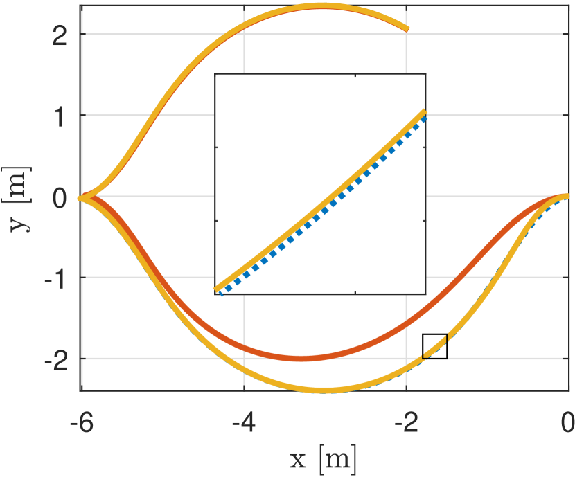
(b) Lemon

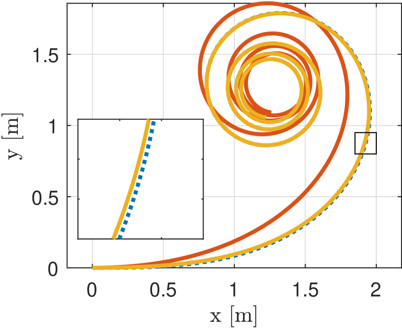
(c) Spiral

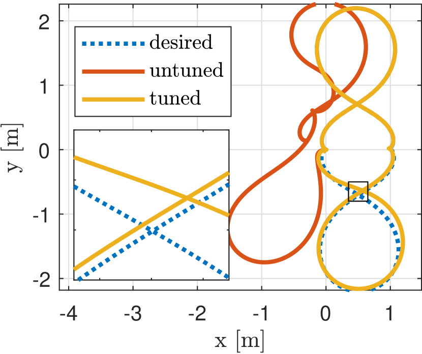
(d) Twist

Figure 4: Comparison of performance between tuned and untuned controller parameters on testing trajectories for generalization.

TABLE I: Testing trajectories for Dubin’s car simulation and associated losses. The average loss of the tuned parameters on the tuning set is 0.36. (The units associated with linear and angular maximum speeds are m/s and rad/s, respectively.)

Trajectory	max speed		loss
	linear	angular	w/ DiffTune	w/o DiffTune
peanut	2	1.3	0.18	63.02
lemon	2	1	0.07	55.18
spiral	1	5	0.39	21.11
twist	2	3.4	2.05	974.57

Generalization: We illustrate the generalization of DiffTune in a batch tuning example. We select nine trajectories (shown in Fig. 11 in Appendix A) as the batch tuning set. These trajectories are generated by composing constant, sinusoidal, and cosinusoidal signals for the desired linear and angular velocities. The maximum linear speed and angular speed are set to 1 m/s and 1 rad/s, respectively, to represent trajectories in one operating region. The four control parameters are all initialized at 2. The tuning proceeds by batch gradient descent on the tuning set. The controller parameters converge to $(k_{\bm{p}},k_{\bm{v}},k_{\psi},k_{\omega})=(18.83,6.69,14.97,2.66)$. We then test the tuned parameters on four testing trajectories (unseen in the tuning set) with lemon-, twist-, peanut-, and spiral-shape, as shown in Fig. 4. The tuned parameters lead to better tracking performance than the untuned ones. The loss on the testing set is compared to the untuned parameters in Table I. It can be observed that the tuned parameters generalize well and are robust to the previously unseen trajectories.

Handling uncertainties: In this simulation, we implement the $\mathcal{L}_{1}$AC to facilitate the compensation for the uncertainties during tuning. For the $\mathcal{L}_{1}$AC, we use the piecewise-constant adaptation law and a 1st-order low-pass filter with 20 rad/s bandwidth. In this simulation, we inject additive force $0.1a_{1}\sin(t)$ and moment $0.1a_{2}\cos(t)$ to the control channels in the dynamics (14) as uncertainties from the environment. To understand how the performance is impacted by the uncertainties, we set $(a_{1},a_{2})$ to a $10\times 10$ grid such that $a_{1}$ and $a_{2}$ take integer values from 1 to 10, representing gradually intensified uncertainties. The four control parameters are all initialized at 10. We tune the controller parameters with both $\mathcal{L}_{1}$ on and $\mathcal{L}_{1}$ off, where the sensitivity propagation in both cases is based on the nominal model in (14). Different from the generalization test, we only tune the parameters on one trajectory (the focus is on how to reduce the impact of the uncertainties that are not considered in the nominal dynamics). The step size and termination criterion remain the same as before. To clearly understand the individual role of DiffTune and the $\mathcal{L}_{1}$AC in tuning, we conduct an ablation study. The losses are shown in Fig. 5. It can be observed that both DiffTune and $\mathcal{L}_{1}$AC improve the performance, and a combination of both achieves the best overall performance: the $\mathcal{L}_{1}$AC does so by compensating for the uncertainties, whereas DiffTune does so by driving the parameters to achieve smaller tracking error. Although the two heatmaps with $\mathcal{L}_{1}$ on show indistinguishable colors within each itself, the actual loss values have minor fluctuations.

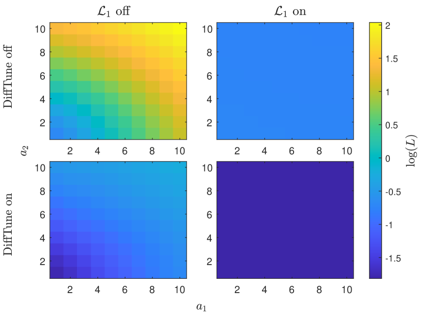
Figure 5: Loss $L$ subject to uncertainties (additive force $0.1a_{1}\sin(t)$ and moment $0.1a_{2}\cos(t)$ with $a_{1}$ and $a_{2}$ taking values from 1 to 10) in the ablation study of DiffTune and $\mathcal{L}_{1}$AC.

V-B Quadrotor

Comparison to other methods: We compare DiffTune with strong baselines AutoTune [12] and SafeOpt-PSO [31]. The latter is a variant of the SafeOpt [9], which applies Particle Swarm Optimization (PSO) to enable adaptive discretization of the parameter space. The original SafeOpt is not applicable because it requires fine discretization of the parameter space to search for the maximizer, which suffers from the curse of dimensionality. Specifically, auto-tuning of the geometric controller requires at least $12^{M}$ discretization points if each parameter admits at least $M$ discretization points. The detailed settings of AutoTune and SafeOpt in this example are shown in Appendix B. We compare the three auto-tuning methods on three trajectories, where 100 trials are performed for each method on each trajectory. The results are shown in Fig. 6. The results are similar to the comparison on Dubin’s car in Fig. 3: DiffTune achieves the minimum tracking RMSE with the best efficiency. Note that the tuning of the quadrotor is more complicated than that of Dubin’s car due to the former’s higher dimensional parameter space and more complicated nonlinearity in dynamics and control. In the tuning on the 2D/3D circular trajectories, the RMSEs show oscillation near the end of the tuning trials, indicating the learning rate might be too large when the loss is close to a (local) minimum. AutoTune and SafeOpt-PSO demonstrate similar performance, where the former has a smoother RMSE reduction than the latter. The final RMSEs achieved by these two baseline auto-tuning methods are close, both inferior to the ones achieved by DiffTune. Moreover, AutoTune and SafeOpt-PSO are less favorable for practical usage since they demand more hyperparameters to be tuned (e.g., the variance of the transition model for each parameter in AutoTune; kernel functions, lower/upper bound of each parameter, safety thresholds, and swarm size for SafeOpt-PSO). In contrast, DiffTune only requires tuning the learning rate as the sole hyperparameter, yet still delivering the best outcome.

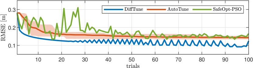
(a) 2D circle

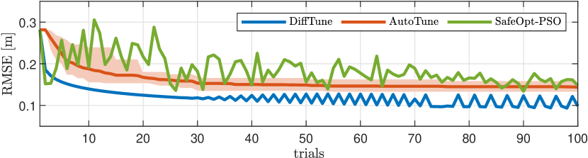
(b) 3D circle

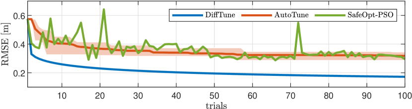
(c) 3D figure 8

Figure 6: Comparison of tuning the controller of a quadrotor using DiffTune (proposed), AutoTune [12], and SafeOpt-PSO [31]. The shaded area shows the range of RMSEs (min to max) achieved in a total of 10 runs of AutoTune.

Handling uncertainties: In this simulation, we consider the uncertainty caused by the imprecise knowledge of the moment of inertia (MoI) $J$. We set the vehicle’s true MoI as $\beta J$ for $\beta$ from 0.5 to 4 and use $J$ in the controller design as our best knowledge of the system. The scaled MoI can be treated as an unknown control input gain (see (16b)), leading to decreased ($\beta>1$) or increased ($\beta<1$) moment in reality compared to the commanded moment by the geometric controller. However, the uncertainty caused by the perturbed MoI can be well handled by $\mathcal{L}_{1}$AC, which is adopted in the simulation (formulation detailed in [52]). We conduct an ablation study to understand the roles of DiffTune and $\mathcal{L}_{1}$AC by comparing the root-mean-square error (RMSE) of position tracking, as shown in Table II (where the tuning is conducted over a 3D figure 8 trajectory in 100 trials with a learning rate of $\alpha=0.005$). It can be seen that tuning and $\mathcal{L}_{1}$ can individually reduce the tracking RMSE. The best performance is achieved when DiffTune and $\mathcal{L}_{1}$AC are applied jointly.

TABLE II: Tracking RMSE [cm] with MoI perturbation $\beta$ ranging from 0.5 to 4 in the ablation study of DiffTune and $\mathcal{L}_{1}$AC. (DT stands for “DiffTune.”)

$\beta$	0.5	1	1.5	2	2.5	3	3.5	4
DT  $\mathcal{L}_{1}$	30.5	30.1	30.8	32.9	34.3	35.4	36.5	37.9
DT  $\mathcal{L}_{1}$	30.8	30.1	31.0	33.9	37.8	39.5	40.5	41.1
DT  $\mathcal{L}_{1}$	57.9	57.5	58.0	59.5	62.2	66.0	70.9	76.8
DT  $\mathcal{L}_{1}$	57.8	57.6	58.9	62.2	67.3	74.1	82.2	90.9

V-C Discussion

The advantage of DiffTune is its efficient usage of the first-order information (gradient $\nabla_{\bm{\theta}}L$) of the target system. Compared with DiffTune, the baseline auto-tuning methods (AutoTune and SafeOpt) have the advantage of tuning without requiring the knowledge of the model (either when the precise model is difficult to establish or when the model/performance metric makes the parameter optimization problem (P) difficult to solve). Both methods use probabilistic approaches (Metropolis-Hastings algorithm and Bayesian optimization) to explore candidates of parameters and iteratively improve the performance based on input-output (i.e., parameters-performance) pairs. However, when the knowledge of the system is obtained through such “sampling” procedures, sufficiently many trials are needed to gain enough information and infer the optimal parameter choice, and the number of trials scales badly with the dimension of the parameter space. However, in practice, many physical systems have models obtained by physics or first principles, which can provide sufficiently useful first-order information to guide parameter searches. Such information will significantly reduce the number of trials in tuning compared to when one uses “sampling” to obtain this information, which is clear in the comparison shown in Figs. 3 and 6. We will illustrate the efficiency of auto-tuning using the first-order information with the experimental results in Section VI next.

VI Experiment results

We validate and evaluate DiffTune on a quadrotor in experiments. We would like to answer the following three questions: 1. How is the performance improvement using DiffTune with only limited tuning budgets (e.g., 10 trials)? 2. How do the tuned parameters generalize to trajectories that are unseen during tuning? 3. What are the individual role of DiffTune and $\mathcal{L}_{1}$AC in terms of performance improvement?

VI-A Experiment setup

We use the same geometric controller as used in Section V-B, where the dynamics and controller can be found in Appendix B. The controller’s initial parameters are shown in Table VI. We only permit 10 tuning trials as the budget to limit the time and mechanical wear of the tuning. The loss function is chosen as the sum of the translational and rotational tracking errors to penalize undesirable tracking performance in these two perspectives, i.e., $L=\lVert\bm{p}-\bar{\bm{p}}\rVert^{2}+\text{tr}(I-\bar{R}^{\top}R)/2$. A horizon of 7 s is used to collect the data and perform sensitivity propagation. The data contains the full state and control actions sampled at 400 Hz (by the design of Ardupilot), where the state is obtained via the original EKF developed by ardupilot, with Vicon providing only position and yaw measurements of the quadrotor. The data are logged onboard and downloaded to a laptop to compute the new controller parameter $\bm{\theta}$. We use learning rate $\alpha=0.1$ together with gradient saturation such that the parameters in the next trial $\bm{\theta}_{j+1}$ will always fall within 10% of the current parameters $\bm{\theta}_{j}$, i.e., $\bm{\theta}_{j+1}\in[0.9\bm{\theta}_{j},1.1\bm{\theta}_{j}]$. Such a saturation scheme is used to (i) prevent the parameters from turning negative when the gradient is large and (ii) enforce a “trust region” around the current parameters to avoid overly large parameter changes. The laptop has an Intel i9-8950HK CPU, and the run time for sensitivity propagation to update the sensitivity states in one iteration (from $k$ to $k+1$) is $91\pm 13\mu$s (in MATLAB).

VI-B Run DiffTune on three trajectories

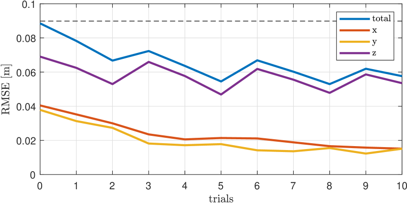
(a) 1 m/s

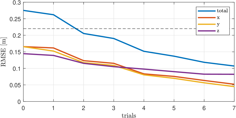
(b) 2 m/s

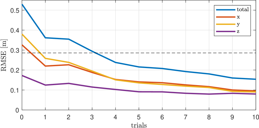
(c) 3 m/s

Figure 7: Tracking error (RMSE) of the tuning on three circular trajectories. The dashed line shows the RMSE achieved by hand-tuning.

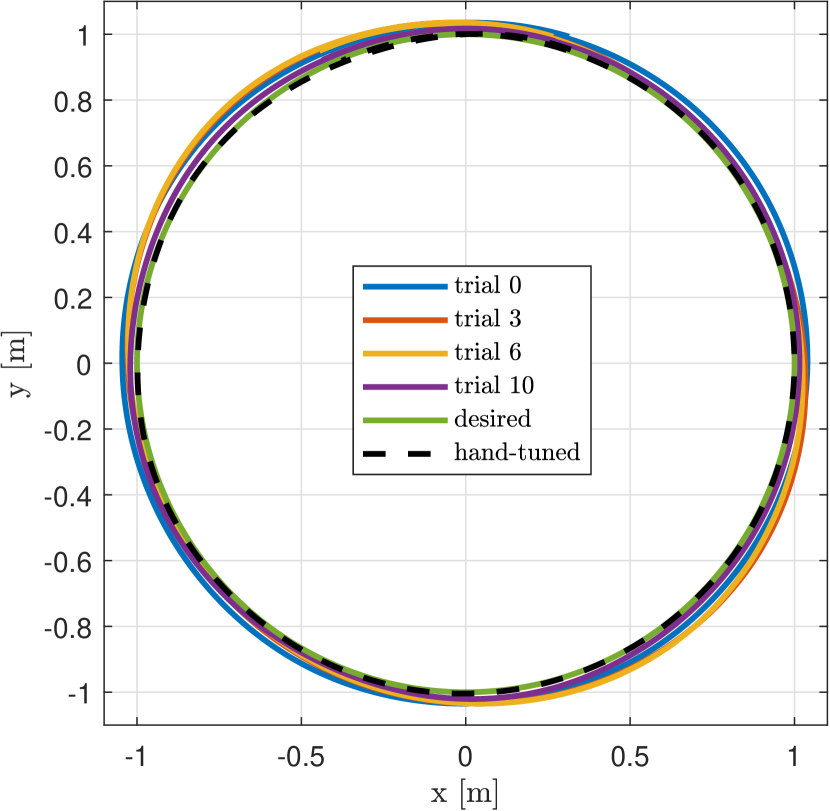
(a) 1 m/s

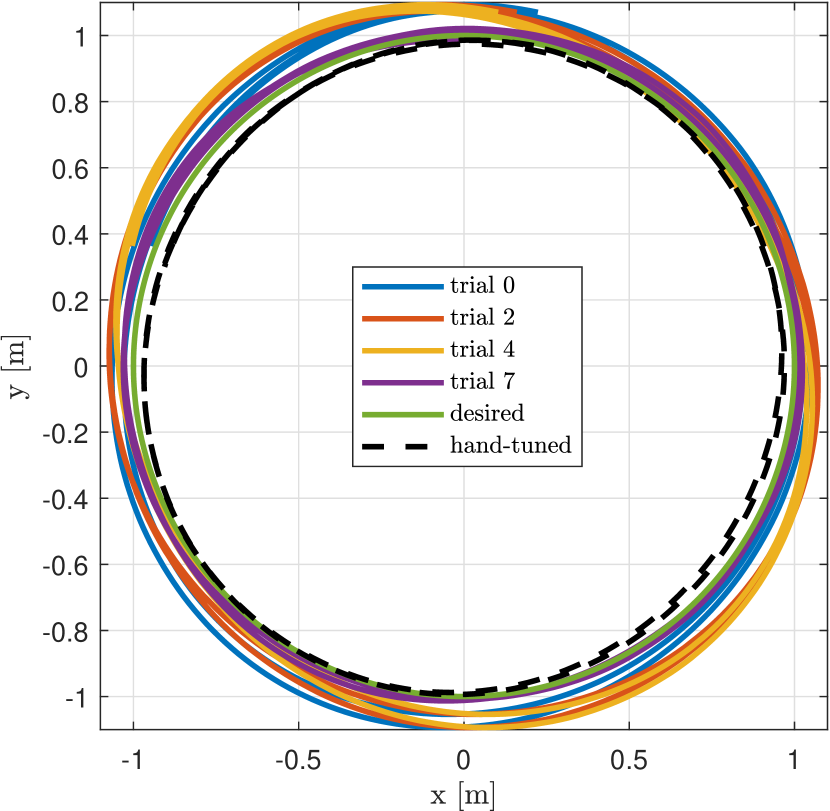
(b) 2 m/s

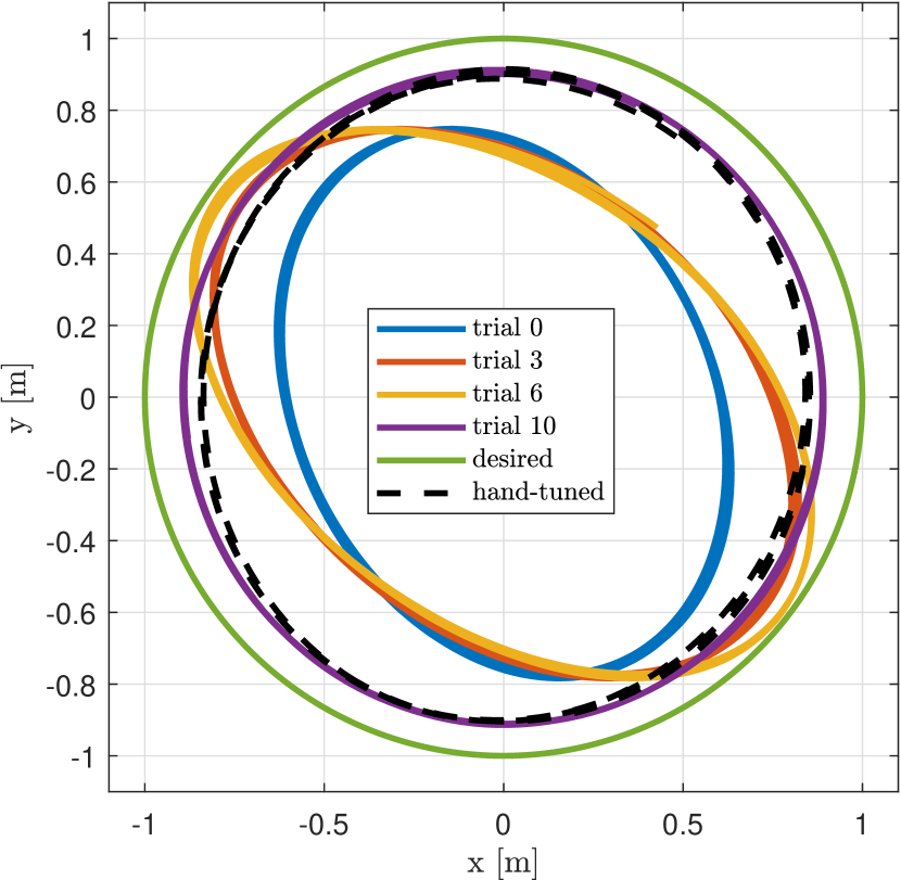
(c) 3 m/s

Figure 8: Horizontal trajectories of the quadrotor during tuning on three circular trajectories with different speeds.

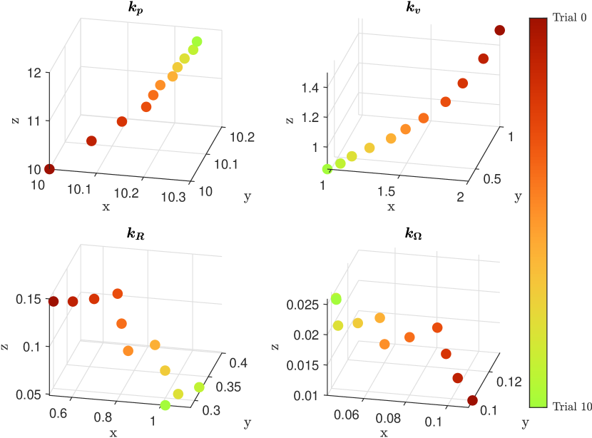
(a) 1 m/s

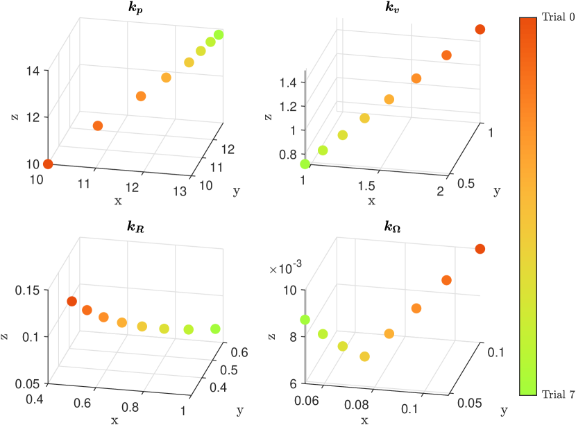
(b) 2 m/s

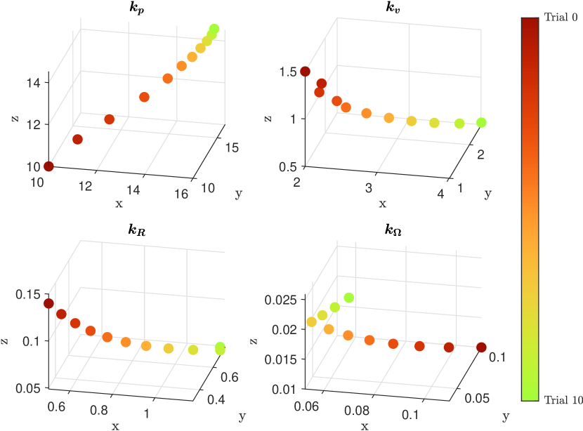
(c) 3 m/s

Figure 9: History of parameters during the tuning on three circular trajectories with different speeds.

We use a circular trajectory for tuning, where the speeds are set to $[1,2,3]$ m/s for a spectrum of agility from slow to aggressive. The controller is tuned individually for these three speeds, and we denote the final parameters by P1, P2, and P3 (associated with the speeds of 1, 2, and 3 m/s, respectively). The parameters P2 are obtained in seven trials because the quadrotor experiences oscillations after the seventh trial, and we decided to use the parameters tuned at the last non-oscillating trial. The reduction of the tracking RMSE is shown in Fig. 7. Comparing the tracking performance at the last trial to the initial trial, the RMSE has achieved 1.5x, 2.5x, and 3.5x reduction on the 1, 2, and 3 m/s circular trajectories, respectively. Furthermore, all the tuned parameters achieve lower tracking RMSEs than the hand-tuned parameters. While the reduction in tracking RMSE is monotone in the 2 and 3 m/s cases, for the case of 1 m/s, a minor fluctuation is superposed on the monotone reduction of the tracking RMSE. This phenomenon happens since the dominant $z$-axis RMSE fluctuates, which is caused by the large learning rate for $z$-axis tracking when the parameters are close to the (local) minimum of $z$-axis error (observe the $z$-axis RMSE reduces only from 6.8 to 5.5 cm). For the $x$- and $y$-axis tracking RMSE, we observe a monotone reduction in all three speeds. Notably, we observe the sensitivity of the angular velocity gains $\bm{k}_{\bm{\Omega}_{x}}$ and $\bm{k}_{\bm{\Omega}_{y}}$ are larger than the other parameters (by at least a magnitude). In other words, the partial derivatives $\partial L/\partial\bm{k}_{\bm{\Omega}_{x}}$ and $\partial L/\partial\bm{k}_{\bm{\Omega}_{y}}$ are large, which leads to significant changes in the gains $\bm{k}_{\bm{\Omega}_{x}}$ and $\bm{k}_{\bm{\Omega}_{y}}$. This reduction leads to a more agile response in rotational tracking on the roll and pitch commands, which efficiently improves the position tracking performance on the $x$- and $y$-axis. The trajectories on the horizontal plane through the tuning trials are shown in Fig. 8. For the 3 m/s circular tuning trajectory, we show the stacked images during the flight in Fig. LABEL:fig:_exp_stacked_images_3mps. It is clear that the quadrotor’s tracking of the circular trajectory becomes better through iterations.

The evolution of the parameters in the tuning trials is shown in Fig. 9. Overall, the parameters tend to converge following one direction, except for the derivative gain $\bm{k}_{\bm{\Omega}}$ for angular tracking. Specifically, near the end of the tuning, $\bm{k}_{\bm{\Omega}}$ shows a change of evolution direction, which indicates that the mapping from these parameters to the loss function is likely to lie on a nonlinear manifold. Such a nonlinear manifold is difficult for a human to perceive and understand in hand-tuning unless sufficiently many, possibly pessimistically unrealistically many, trials are provided, which leads to the challenges in tuning a nonlinear controller by hand. Furthermore, another challenge of hand tuning is that one may alter one or (at most) two parameters in each trial since humans essentially perform coordinate-wise finite differences via trial and error to tune the controller. These two factors combined result in inefficient tuning by hand, especially when the dimension of parameter space is high (e.g., 12 for the geometric control [59]). We display the tuned parameters in Table VI in Appendix C, along with the initial parameters and hand-tuned parameters for comparison.

VI-C Generalization

We conducted experiments to test the generalization capability of the tuned parameters in Section VI-B. The testing set contains circular, 3D figure 8, and vertical figure 8 trajectories, with their coordinates shown in Table III and shapes shown in Fig. 13 (in the Appendix C). The latter two trajectories are considered here for their wide range of speed and acceleration (see Table IV), which is in contrast to those static values of the circular trajectories. We test the three groups of tuned parameters P1, P2, and P3 on circular trajectories with 1, 2, and 3 m/s speed, respectively. The tracking performance of these tuned parameters on the testing trajectories is shown in Table IV, in which we also include the baseline of hand-tuned parameters.

TABLE III: Trajectories used in the generalizability study. The trajectories are parameterized by $v$, and their $xyz$-coordinates are shown in the “Function” column ($t$ is the time argument).

Trajectory	Notation	Function
		$x(t)=\sin(vt)$
Circular	$C(v)$	$y(t)=-\cos(vt)$
		$z(t)=-1$
		$x(t)=1.5\sin(vt/1.75)$
3D figure 8	$DF(v)$	$y(t)=\sin(2vt/1.75)$
		$z(t)=-1-0.3\sin(0.5vt/1.75)$
		$x(t)=1.5\sin(vt/1.25)$
Vertical figure 8	$VF(v)$	$y(t)=\sin(vt/1.25)$
		$z(t)=-1-0.3\sin(2vt/1.25)$

TABLE IV: Tracking RMSE [cm] in the generalizability test. The star indicates minor oscillations on the pitch angle of the quadrotor. “HT” stands for hand-tuned.

Traj.	Spd.	Acc.	P1	P2	P3	HT
unit	[m/s]	[m/s2]	[cm]	[cm]	[cm]	[cm]
$C(1)$	1	1	5.7	5.7	5.5*	9.0
$C(2)$	2	4	27.2	10.7	16.6	18.0
$C(3)$	3	9	72.8	31.7	15.4	28.6
$DF(1)$	0.59–1.43	0.00–1.35	5.5	4.9	4.8*	5.3
$DF(2)$	1.17–2.86	0.00–5.41	10.6	8.8	8.3	9.2
$VF(1)$	0.48–1.52	0.00–1.20	12.5	10.5	9.7*	9.6
$VF(2)$	0.96–3.04	0.00–4.81	17.8	13.0	9.8	12.7

When tested on the circular trajectories: the tuned parameters perform the best on the speed that they were tuned for, i.e., P$n$ performs the best on trajectory $C(n)$ for $n\in\{1,2,3\}$. The same phenomenon has been observed in [12] (although the controller therein is different from the one used here), where parameters perform the best over the trajectories that they are tuned on. This behavior is similar to an overfitted NN in machine learning. In our case, this type of “overfitting” is expected since the proportional-derivative structure of the geometric controller determines that there does not exist a group of parameters that work well for all conditions (e.g., the aggressive trajectory $C(3)$ demands a distinct parameter combination than for the slow trajectory $C(1)$). However, the parameters can still generalize to the 3D figure 8 and vertical figure 8 trajectories that are not used for tuning. Specifically, P2 and P3, which are tuned for increasingly aggressive maneuvers with fast-changing directions of velocity and acceleration, generalize to the two variants of the figure 8 trajectory that demands fast-changing speed and acceleration. P3 demonstrates better agility, which shows the best performance on $DF(2)$ and $VF(2)$. However, P3 is overly agile for the speed and acceleration in $DF(1)$ and $VF(1)$, which leads to minimum RMSE compared to P1 and P2, albeit with minor oscillations on the pitch angle.

VI-D Ablation Study

We conduct an ablation study of how much contribution DiffTune and $\mathcal{L}_{1}$AC provide to performance improvement. We repeat the tuning in Section VI-B but with $\mathcal{L}_{1}$AC in the loop, which results in different sets of parameters for the three trajectories denoted by Pn-$\mathcal{L}_{1}$ for $n\in\{1,2,3\}$ and shown in Table VI in Appendix C. Our implementation follows [60]. Unlike the simulations in Section V-B where we deliberately introduce uncertainties in MoI, in the experiment, we do not introduce uncertainties. The quadrotor naturally has uncertainties existing in the system (e.g., varying battery voltage in flight and mismatch between the actual MoI and estimated MoI through CAD computation), in which case $\mathcal{L}_{1}$AC can help compensate for these uncertainties and thus improve the tracking performance. The results are shown in Table V. Here, “DiffTune off” shows the performance of the initial parameters (no tuning occurs); “DiffTune on” shows the tracking performance in the final tuning trial. “$\mathcal{L}_{1}$ on/off” indicate whether $\mathcal{L}_{1}$AC is used or not during the tuning trials. We conclude that 1. DiffTune alone can improve the tracking performance, albeit the system has uncertainties and measurement noise. 2. When $\mathcal{L}_{1}$AC is combined with DiffTune, $\mathcal{L}_{1}$AC helps improve the performance in two ways: (i) compensating for the uncertainties so that the uncertainties’ degradation to system performance is mitigated; and (ii) DiffTune can proceed with less biased gradient thanks to the uncertainties being “canceled out” by $\mathcal{L}_{1}$AC, which leads to more efficient tuning. Intuitively, DiffTune raises the performance’s upper limit (in an ideal case subject to no uncertainty), whereas $\mathcal{L}_{1}$AC keeps the actual performance (in a realistic case subject to uncertainties) close to the upper limit. When the two are used together, the best performance is achieved.

TABLE V: Tracking RMSE [cm] in ablation study with DiffTune and $\mathcal{L}_{1}$AC.

Speed [m/s]		1		2		3
$\mathcal{L}_{1}$AC		off	on	off	on	off	on
DiffTune	off	8.9	7.5	27.5	25.1	61.8	46.6
	on	5.7	3.0	10.7	6.9	17.7	16.2

VII Conclusion

In this paper, we propose DiffTune: an auto-tuning method using auto-differentiation, with the advantage of stability, compatibility with data from physical systems, and efficiency. Given a performance metric, DiffTune gradually improves the performance using gradient descent, where the gradient is computed using sensitivity propagation that is compatible with physical systems’ data. We also show how to use $\mathcal{L}_{1}$AC to mitigate the discrepancy between the nominal model and the associated physical system when the latter suffers from uncertainties. Simulation results (on a Dubin’s car and a quadrotor) and experimental results (on a quadrotor) both show that DiffTune can efficiently improve the system’s performance. When uncertainties are present in a system, $\mathcal{L}_{1}$ adaptive control facilitates tuning by compensating for the uncertainties. Generalization of the tuned parameters to unseen trajectories during tuning is also illustrated in both simulation and experiments.

One limitation of the proposed approach is that it only applies to systems with differentiable dynamics and controllers. The requirement on differentiability is not met in contact-rich applications [61] (e.g., legged robots [62] and dexterous manipulation [63]) and systems with actuation limits [7] (e.g., saturations in magnitude or changing rate). Although subgradients [64] generally exist at the points of discontinuity, the impact of surrogate gradient on the tuning efficiency is unknown, which will be investigated in the future.

Appendix

VII-A Details of the Dubin’s car simulation

Dynamics and controller: Consider the following nonlinear model:

$$\dot{x}(t)=v(t)\cos(\psi(t)),\ \dot{y}(t)=v(t)\sin(\psi(t)),$$ (14a)

$$\dot{\psi}(t)=\omega(t),\ \dot{v}(t)=F(t)/m,\ \dot{w}(t)=M(t)/J,$$ (14b)

where the state contains five scalar variables, $(x,y,\psi,v,w)$, which stand for horizontal position, vertical position, yaw angle, linear speed in the forward direction, and angular speed. The control actions in this model include the force $F\in\mathbb{R}$ in the forward direction of the vehicle and the moment $M\in\mathbb{R}$. The vehicle’s mass and moment of inertia are known and denoted by $m$ and $J$, respectively. The feedback tracking controller with tunable parameter $\bm{\theta}=(k_{\bm{p}},k_{\bm{v}},k_{\psi},k_{\omega})$ is given by

$$F(t)= m(k_{\bm{p}}\bm{e}_{\bm{p}}(t)+k_{\bm{v}}\bm{e}_{\bm{v}}(t)+\dot{\bar{\bm{v}}}(t))^{\top}\bm{q}(t),$$ (15a)

$$M(t)= J(k_{\psi}e_{\psi}(t)+k_{\omega}e_{\omega}(t)+\dot{\bar{{\omega}}}(t)),$$ (15b)

where $\bar{\cdot}$ indicates the desired value, the error terms are defined by $\bm{e}_{\bm{p}}=\bar{\bm{p}}-\bm{p}$, $\bm{e}_{\bm{v}}=\bar{\bm{v}}-\bm{v}$, $e_{\psi}=\bar{\psi}-\psi$, and $e_{\omega}=\bar{\omega}-\omega$ for $\bm{p}$ and $\bm{v}$ being the 2-dimensional vector of position and velocity, respectively, $\bm{q}=[\cos(\psi)\ \sin(\psi)]^{\top}$ being the heading of the vehicle, $\bar{\bm{v}}=[\bar{v}\cos(\bar{\psi})\ \bar{v}\sin(\bar{\phi})]^{\top}$ and $\dot{\bar{\bm{v}}}$ being the desired linear velocity and acceleration, respectively. The control law (15) is a PD controller with proportional gains $(k_{\bm{p}},k_{\psi})$ and derivative gains $(k_{\bm{v}},k_{\omega})$. If $\bm{\theta}>0$, then this controller is exponentially stable for the tracking errors $(\lVert\bm{e}_{\bm{p}}\rVert,\lVert\bm{e}_{\bm{v}}\rVert,\lVert e_{\psi}\rVert,\lVert e_{\omega}\rVert)$. We set the loss function is the squared norm of the position tracking error, summed over a horizon of 10 s.

Tuning setup: For Autotune [12], we use a Gaussian distribution with variances set to 1 to sample the four parameters iteratively. The scoring function is the exponential of the tracking RMSE. Since sampling is used in AutoTune, we conduct 10 runs and show the mean, max, and min RMSEs in Fig. 3. For SafeOpt, we choose the standard radial basis function kernel for GP. The safety threshold is set to 1 m RMSE. For DiffTune, we use a learning rate $\alpha=1$. (The tracking RMSE’s reduction with different learning rates in Dubin’s car example is shown in Fig. 10, which is consistent with how learning rate influences the loss reduction in general in a gradient-descent algorithm.) The feasible set of each parameter is set to $[1,20]$ and applies to all three methods compared.

For the batch tuning for generalization, we choose $\alpha=0.1$ as the learning rate in the gradient descent algorithm and choose the termination condition as the relative reduction in the total loss between two consecutive steps being smaller than 1e-4 of the current loss value.

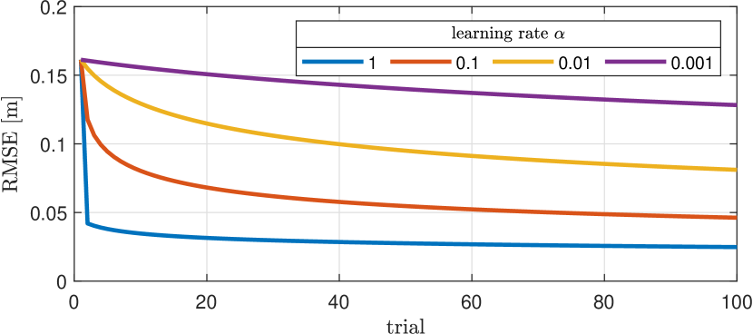
Figure 10: Performance of DiffTune in Dubin’s car example with different learning rates.

The trajectories used for batch tuning for Dubin’s car are shown in Fig. 11, where the tuned parameters can achieve acceptable tracking on these trajectories.

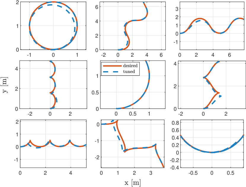
Figure 11: Trajectories for batch tuning in Dubin’s car example.

VII-B Details of the quadrotor simulation

Formulation: Consider the following model on SE(3):

$$\dot{\bm{p}}=\bm{v},\quad \dot{\bm{v}}=g\bm{e}_{3}-\frac{f}{m}R\bm{e}_{3},$$ (16a)

$$\dot{R}=R\bm{\Omega}^{\times},\quad \dot{\bm{\Omega}}=J^{-1}(\bm{M}-\bm{\Omega}\times J\bm{\Omega}),$$ (16b)

where $\bm{p}\in\mathbb{R}^{3}$ and $\bm{v}\in\mathbb{R}^{3}$ are the position and velocity of the quadrotor, respectively, $R\in SO(3)$ is the rotation matrix describing the quadrotor’s attitude, ${\bm{\Omega}\in\mathbb{R}^{3}}$ is the angular velocity, $g$ is the gravitational acceleration, $m$ is the vehicle mass, $J\in\mathbb{R}^{3\times 3}$ is the moment of inertia (MoI) matrix, $f$ is the collective thrust, and $\bm{M}\in\mathbb{R}^{3}$ is the moment applied to the vehicle. The wedge operator $\cdot^{\times}:\mathbb{R}^{3}\rightarrow\mathfrak{so}(3)$ denotes the mapping to the space of skew-symmetric matrices. The control actions $f$ and $\bm{M}$ are computed using the geometric controller [59]. The geometric controller has a 12-dimensional parameter space, which splits into four groups of parameters: $\bm{k}_{\bm{p}}$, $\bm{k}_{\bm{v}}$, $\bm{k}_{R}$, $\bm{k}_{\bm{\Omega}}$ (applying to the tracking errors in position, linear velocity, attitude, and angular velocity, respectively). Each group is a 3-dimensional vector (associated with the $x$-, $y$-, and $z$-component in each’s corresponding tracking error). The initial parameters for tuning are set as $\bm{k}_{\bm{p}}=16\mathbb{I}$, $\bm{k}_{\bm{v}}=5.6\mathbb{I}$, $\bm{k}_{R}=8.81\mathbb{I}$, and $\bm{k}_{\bm{\Omega}}=2.54\mathbb{I}$, for $\mathbb{I}=[1,1,1]^{\top}$. The feasible sets of controller parameters are set as $\bm{k}_{\bm{p}}\in[15,24]$, $\bm{k}_{\bm{v}}\in[4,16]$, $\bm{k}_{\bm{R}}\in[8,12]$, and $\bm{k}_{\bm{\Omega}}\in[0.1,3]$. We set the loss function as the squared norm of the position tracking error, summed over a horizon of 10 s. We add zero-mean Gaussian noise to the position, linear velocity, and angular velocity (with standard deviation 0.1 m, 0.1 m/s, 1e-3 rad/s, respectively).

TABLE VI: Comparison of the initial parameters, DiffTune final parameters (P1, P2, and P3), DiffTune-$\mathcal{L}_{1}$AC final parameters (P1-$\mathcal{L}_{1}$, P2-$\mathcal{L}_{1}$, and P3-$\mathcal{L}_{1}$), and hand-tuned parameters

Param.	$\bm{k}_{\bm{p}}$			$\bm{k}_{\bm{v}}$			$\bm{k}_{R}$			$\bm{k}_{\bm{\Omega}}$
axis	$x$	$y$	$z$	$x$	$y$	$z$	$x$	$y$	$z$	$x$	$y$	$z$
initial	10	10	10	2	1	1.5	0.5	0.3	0.14	0. 11	0.1	0.01
P1	10.25	10.20	11.72	0.97	0.35	0.85	1.02	0.29	0.05	0.05	0.10	0.03
P2	12.91	12.92	13.75	0.96	0.48	0.72	0.97	0.58	0.07	0.05	0.05	0.01
P3	15.56	16.62	14.54	4.01	2.59	0.52	1.16	0.78	0.05	0.07	0.03	0.03
P1-$\mathcal{L}_{1}$	10.52	10.44	10.04	0.71	0.34	1.40	1.15	0.67	0.13	0.06	0.04	0.03
P2-$\mathcal{L}_{1}$	11.79	11.77	12.14	0.96	0.48	0.72	0.97	0.58	0.22	0.05	0.05	0.01
P3-$\mathcal{L}_{1}$	16.29	16.11	16.26	1.27	0.95	0.52	1.29	0.77	0.05	0.07	0.04	0.03
hand-tuned	14	15	15	1.50	0.90	1.10	0.55	0.35	0.15	0.04	0.03	0.01

Tuning setup: For AutoTune [12], the variances of Gaussian distribution in the transition model are set to 2 for $\bm{k}_{\bm{p}}$, $\bm{k}_{\bm{v}}$, and $\bm{k}_{\bm{R}}$ and 1 for $\bm{k}_{\bm{\Omega}}$. The scoring function is the exponential of the RMSE trackign error. For the SafeOpt-PSO [31], we choose Matérn kernel with parameter $\nu=5/2$ and set safety threshold to be as 1 m RMSE. While following the default setting therein, we increase the swarm size to 400, considering the complexity of our problem. For DiffTune, the learning rate is set to 0.1. The same feasible set of parameters and horizon of sampling are used in all three methods.

For Difftune, we tested three learning rates of $\alpha\in\{0.1,\ 0.01,\ 0.001\}$. The results are shown in Fig. 12, where the rate of loss reduction is positively correlated to the magnitude of the learning rate. Furthermore, oscillation in the loss value is observed when $\alpha$ is relatively large (0.1), indicating the learning rate is too large when the parameters are close to the (local) minimum. These observations are consistent with how the learning rate influences the loss reduction in gradient descent.

In the ablation study of $\mathcal{L}_{1}$AC and DiffTune, we relax the upper bound on the feasible parameters so that the parameters can grow to higher values to handle the uncertainties.

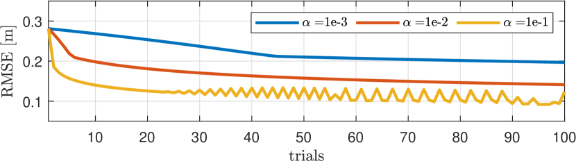
(a) 2D circle

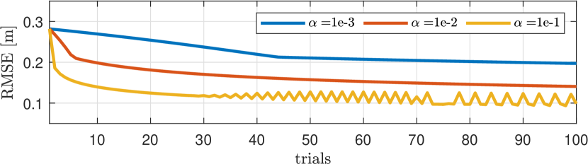
(b) 3D circle

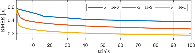
(c) 3D figure 8

Figure 12: Loss reduction by DiffTune under different learning rates $\alpha$ in the quadrotor simulation.

VII-C Details of the quadrotor experiment

We use a custom-built quadrotor to conduct the experiments. The quadrotor weighs 0.63 kg with a 0.22 m diagonal motor-to-motor distance. The quadrotor is controlled by a Pixhawk 4 mini flight controller running the ArduPilot firmware. We modify the firmware to enable the geometric controller and the $\mathcal{L}_{1}$ adaptive control, which both run at 400 Hz on the Pixhawk. Position feedback is provided by 9 Vicon V16 cameras. We use ArduPilot’s EKF to fuse the Vicon measurements with IMU readings onboard.

The tuned parameters, without and with $\mathcal{L}_{1}$AC in the loop, are shown in Table VI. The trajectories used for testing generalization in Table III are shown in Fig. 13.

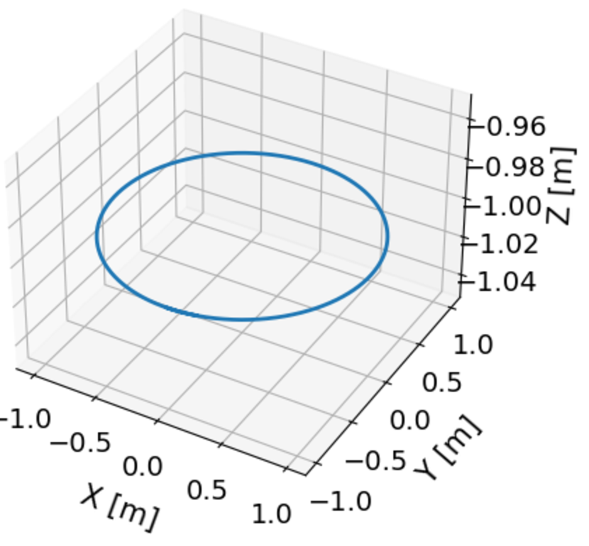
(a) Circle

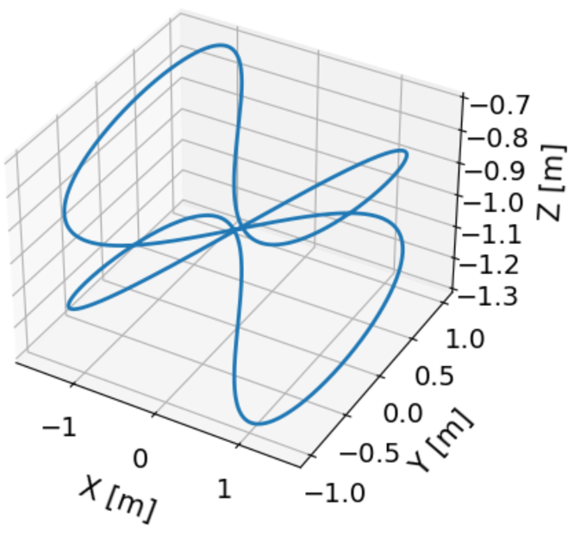
(b) 3D figure 8

(c) Vertical figure 8

Figure 13: Trajectories used in the generalization test.

References

- [1] A. O’dwyer, Handbook of PI and PID controller tuning rules. Singapore: World Scientific, 2009.
- [2] C.-C. Yu, Autotuning of PID controllers: A relay feedback approach. Berlin, Germany: Springer, 2006.
- [3] K. J. Åström, T. Hägglund, C. C. Hang, and W. K. Ho, “Automatic tuning and adaptation for PID controllers - a survey,” Control Engineering Practice, vol. 1, no. 4, pp. 699–714, 1993.
- [4] Y. Li, K. H. Ang, and G. C. Chong, “Patents, software, and hardware for PID control: an overview and analysis of the current art,” IEEE Control Systems Magazine, vol. 26, no. 1, pp. 42–54, 2006.
- [5] M. Zhuang and D. Atherton, “Automatic tuning of optimum PID controllers,” in IEE Proceedings D (Control Theory and Applications), vol. 140, no. 3. IET Digital Library, 1993, pp. 216–224.
- [6] S. Trimpe, A. Millane, S. Doessegger, and R. D’Andrea, “A self-tuning LQR approach demonstrated on an inverted pendulum,” IFAC Proceedings Volumes, vol. 47, no. 3, pp. 11 281–11 287, 2014.
- [7] A. R. Kumar and P. J. Ramadge, “DiffLoop: Tuning PID controllers by differentiating through the feedback loop,” in Proceedings of the 55th Annual Conference on Information Sciences and Systems, Baltimore, MD, USA, 2021, pp. 1–6.
- [8] A. Marco, P. Hennig, J. Bohg, S. Schaal, and S. Trimpe, “Automatic LQR tuning based on Gaussian process global optimization,” in Proceedings of IEEE International Conference on Robotics and Automation, Stockholm, Sweden, 2016, pp. 270–277.
- [9] F. Berkenkamp, A. P. Schoellig, and A. Krause, “Safe controller optimization for quadrotors with Gaussian processes,” in Proceedings of IEEE International Conference on Robotics and Automation, Stockholm, Sweden, 2016, pp. 491–496.
- [10] R. Calandra, N. Gopalan, A. Seyfarth, J. Peters, and M. P. Deisenroth, “Bayesian gait optimization for bipedal locomotion,” in Proceedings of the International Conference on Learning and Intelligent Optimization, Gainesville, FL, USA, 2014, pp. 274–290.
- [11] D. J. Lizotte, T. Wang, M. H. Bowling, and D. Schuurmans, “Automatic gait optimization with Gaussian Process Regression,” in Proceedings of the International Joint Conferences on Artificial Intelligence Organization, vol. 7, Hyderabad, India, 2007, pp. 944–949.
- [12] A. Loquercio, A. Saviolo, and D. Scaramuzza, “AutoTune: Controller tuning for high-speed flight,” IEEE Robotics and Automation Letters, vol. 7, no. 2, pp. 4432–4439, 2022.
- [13] M. Mehndiratta, E. Camci, and E. Kayacan, “Can deep models help a robot to tune its controller? A step closer to self-tuning model predictive controllers,” Electronics, vol. 10, no. 18, p. 2187, 2021.
- [14] R. Moriconi, M. P. Deisenroth, and K. Sesh Kumar, “High-dimensional Bayesian optimization using low-dimensional feature spaces,” Machine Learning, vol. 109, pp. 1925–1943, 2020.
- [15] B. Amos and J. Z. Kolter, “OptNet: Differentiable optimization as a layer in neural networks,” in Proceedings of the 34th International Conference on Machine Learning, Sydney, Australia, 2017, pp. 136–145.
- [16] B. Amos, I. Jimenez, J. Sacks, B. Boots, and J. Z. Kolter, “Differentiable MPC for end-to-end planning and control,” in Proceedings of the 32nd Conference on Neural Information Processing Systems, vol. 31, Montreal, Canada, 2018.
- [17] S. East, M. Gallieri, J. Masci, J. Koutnik, and M. Cannon, “Infinite-horizon differentiable model predictive control,” in Proceedings of the International Conference on Learning Representations, Online, 2020.
- [18] W. Jin, Z. Wang, Z. Yang, and S. Mou, “Pontryagin differentiable programming: An end-to-end learning and control framework,” in Proceedings of the 34th Conference on Neural Information Processing Systems, vol. 33, Vancouver, Canada, 2020, pp. 7979–7992.
- [19] W. Jin, T. D. Murphey, D. Kulić, N. Ezer, and S. Mou, “Learning from sparse demonstrations,” IEEE Transactions on Robotics, 2022.
- [20] H. Ma, B. Zhang, M. Tomizuka, and K. Sreenath, “Learning differentiable safety-critical control using control barrier functions for generalization to novel environments,” arXiv:2201.01347, 2022.
- [21] W. Xiao, R. Hasani, X. Li, and D. Rus, “BarrierNet: A safety-guaranteed layer for neural networks,” arXiv:2111.11277, 2021.
- [22] W. Xiao, T.-H. Wang, M. Chahine, A. Amini, R. Hasani, and D. Rus, “Differentiable control barrier functions for vision-based end-to-end autonomous driving,” arXiv:2203.02401, 2022.
- [23] H. Parwana and D. Panagou, “Recursive feasibility guided optimal parameter adaptation of differential convex optimization policies for safety-critical systems,” arXiv:2109.10949, 2021.
- [24] N. A. Vien and G. Neumann, “Differentiable robust LQR layers,” arXiv:2106.05535, 2021.
- [25] A. Paszke, S. Gross, F. Massa, A. Lerer, J. Bradbury, G. Chanan, T. Killeen, Z. Lin, N. Gimelshein, L. Antiga, A. Desmaison, A. Kopf, E. Yang, Z. DeVito, M. Raison, A. Tejani, S. Chilamkurthy, B. Steiner, L. Fang, J. Bai, and S. Chintala, “PyTorch: An imperative style, high-performance deep learning library,” in Proceedings of the 33rd Conference on Neural Information Processing Systems, Vancouver, Canada, 2019, pp. 8024–8035.
- [26] M. Abadi, A. Agarwal, P. Barham, E. Brevdo, Z. Chen, C. Citro, G. S. Corrado, A. Davis, J. Dean, M. Devin, S. Ghemawat, I. Goodfellow, A. Harp, G. Irving, M. Isard, Y. Jia, R. Jozefowicz, L. Kaiser, M. Kudlur, J. Levenberg, D. Mané, R. Monga, S. Moore, D. Murray, C. Olah, M. Schuster, J. Shlens, B. Steiner, I. Sutskever, K. Talwar, P. Tucker, V. Vanhoucke, V. Vasudevan, F. Viégas, O. Vinyals, P. Warden, M. Wattenberg, M. Wicke, Y. Yu, and X. Zheng, “TensorFlow: Large-scale machine learning on heterogeneous systems,” arXiv:1603.04467, 2016.
- [27] J. Bradbury, R. Frostig, P. Hawkins, M. J. Johnson, C. Leary, D. Maclaurin, G. Necula, A. Paszke, J. VanderPlas, S. Wanderman-Milne, and Q. Zhang, “JAX: composable transformations of Python+NumPy programs,” 2018. [Online]. Available: http://github.com/google/jax
- [28] J. A. E. Andersson, J. Gillis, G. Horn, J. B. Rawlings, and M. Diehl, “CasADi – A software framework for nonlinear optimization and optimal control,” Mathematical Programming Computation, vol. 11, no. 1, pp. 1–36, 2019.
- [29] H. K. Khalil, Nonlinear Control. London, United Kingdom: Pearson, 2015, vol. 406.
- [30] N. Hovakimyan and C. Cao, Adaptive Control Theory: Guaranteed Robustness with Fast Adaptation. Philadelphia, PA, USA: SIAM, 2010.
- [31] R. R. Duivenvoorden, F. Berkenkamp, N. Carion, A. Krause, and A. P. Schoellig, “Constrained bayesian optimization with particle swarms for safe adaptive controller tuning,” IFAC-PapersOnLine, vol. 50, no. 1, pp. 11 800–11 807, 2017.
- [32] J. C. Spall, Introduction to Stochastic Search and Optimization: Estimation, Simulation, and Control. Hoboken, NJ, USA: Wiley, 2005.
- [33] A. Romero, S. Sun, P. Foehn, and D. Scaramuzza, “Model predictive contouring control for time-optimal quadrotor flight,” IEEE Transactions on Robotics, vol. 38, no. 6, pp. 3340–3356, 2022.
- [34] A. Romero, Y. Song, and D. Scaramuzza, “Actor-critic model predictive control,” arXiv preprint arXiv:2306.09852, 2023.
- [35] N. J. Killingsworth and M. Krstic, “PID tuning using extremum seeking: online, model-free performance optimization,” IEEE Control Systems Magazine, vol. 26, no. 1, pp. 70–79, 2006.
- [36] W. K. Hastings, “Monte carlo sampling methods using markov chains and their applications,” 1970.
- [37] W. Edwards, G. Tang, G. Mamakoukas, T. Murphey, and K. Hauser, “Automatic tuning for data-driven model predictive control,” in Proceedings of the IEEE International Conference on Robotics and Automation, Xi’an, China, 2021, pp. 7379–7385.
- [38] G. Brockman, V. Cheung, L. Pettersson, J. Schneider, J. Schulman, J. Tang, and W. Zaremba, “Openai gym,” 2016.
- [39] M. A. Gelbart, J. Snoek, and R. P. Adams, “Bayesian optimization with unknown constraints,” arXiv preprint arXiv:1403.5607, 2014.
- [40] F. Berkenkamp, A. Krause, and A. P. Schoellig, “Bayesian optimization with safety constraints: safe and automatic parameter tuning in robotics,” Machine Learning, pp. 1–35, 2021.
- [41] A. S. Polydoros and L. Nalpantidis, “Survey of model-based reinforcement learning: Applications on robotics,” Journal of Intelligent & Robotic Systems, vol. 86, no. 2, pp. 153–173, 2017.
- [42] F. Tambon, G. Laberge, L. An, A. Nikanjam, P. S. N. Mindom, Y. Pequignot, F. Khomh, G. Antoniol, E. Merlo, and F. Laviolette, “How to certify machine learning based safety-critical systems? A systematic literature review,” Automated Software Engineering, vol. 29, no. 2, pp. 1–74, 2022.
- [43] H. Ravichandar, A. S. Polydoros, S. Chernova, and A. Billard, “Recent advances in robot learning from demonstration,” Annual Review of Control, Robotics, and Autonomous Systems, vol. 3, pp. 297–330, 2020.
- [44] J.-X. Xu, “A survey on iterative learning control for nonlinear systems,” International Journal of Control, vol. 84, no. 7, pp. 1275–1294, 2011.
- [45] D. A. Bristow, M. Tharayil, and A. G. Alleyne, “A survey of iterative learning control,” IEEE control systems magazine, vol. 26, no. 3, pp. 96–114, 2006.
- [46] L. Brunke, M. Greeff, A. W. Hall, Z. Yuan, S. Zhou, J. Panerati, and A. P. Schoellig, “Safe learning in robotics: From learning-based control to safe reinforcement learning,” Annual Review of Control, Robotics, and Autonomous Systems, vol. 5, pp. 411–444, 2022.
- [47] R. D. Neidinger, “Introduction to automatic differentiation and matlab object-oriented programming,” SIAM review, vol. 52, no. 3, pp. 545–563, 2010.
- [48] A. G. Baydin, B. A. Pearlmutter, A. A. Radul, and J. M. Siskind, “Automatic differentiation in machine learning: a survey,” Journal of Marchine Learning Research, vol. 18, pp. 1–43, 2018.
- [49] N. Parikh, S. Boyd et al., “Proximal algorithms,” Foundations and Trends® in Optimization, vol. 1, no. 3, pp. 127–239, 2014.
- [50] S. Cheng, L. Song, M. Kim, S. Wang, and N. Hovakimyan, “Difftune+: Hyperparameter-free auto-tuning using auto-differentiation,” in Learning for Dynamics and Control Conference. PMLR, 2023, pp. 170–183.
- [51] X. Wang and N. Hovakimyan, “ adaptive controller for nonlinear time-varying reference systems,” Systems & Control Letters, vol. 61, no. 4, pp. 455–463, 2012.
- [52] Z. Wu, S. Cheng, K. A. Ackerman, A. Gahlawat, A. Lakshmanan, P. Zhao, and N. Hovakimyan, “ adaptive augmentation for geometric tracking control of quadrotors,” in Proceedings of the International Conference on Robotics and Automation, Philadelphia, PA, USA, 2022, pp. 1329–1336.
- [53] J. Pravitra, K. A. Ackerman, C. Cao, N. Hovakimyan, and E. A. Theodorou, “-adaptive MPPI architecture for robust and agile control of multirotors,” in Proceedings of the IEEE/RSJ International Conference on Intelligent Robot and Systems, Las Vegas, NV, USA, 2020.
- [54] D. Hanover, P. Foehn, S. Sun, E. Kaufmann, and D. Scaramuzza, “Performance, precision, and payloads: Adaptive nonlinear MPC for quadrotors,” IEEE Robotics and Automation Letters, vol. 7, no. 2, pp. 690–697, 2021.
- [55] P. Zhao, Y. Mao, C. Tao, N. Hovakimyan, and X. Wang, “Adaptive robust quadratic programs using control lyapunov and barrier functions,” in 2020 59th IEEE Conference on Decision and Control (CDC). IEEE, 2020, pp. 3353–3358.
- [56] Z. Wu, S. Cheng, P. Zhao, A. Gahlawat, K. A. Ackerman, A. Lakshmanan, C. Yang, J. Yu, and N. Hovakimyan, “Quad: adaptive augmentation of geometric control for agile quadrotors with performance guarantees,” arXiv preprint arXiv:2302.07208, 2023.
- [57] A. Gahlawat, A. Lakshmanan, L. Song, A. Patterson, Z. Wu, N. Hovakimyan, and E. A. Theodorou, “Contraction -adaptive control using Gaussian processes,” in Proceedings of the 3rd Conference on Learning for Dynamics and Control, vol. 144, Online, 07 – 08 June 2021, pp. 1027–1040.
- [58] S. Cheng, L. Song, and M. Kim. [Online]. Available: https://github.com/Sheng-Cheng/DiffTuneOpenSource
- [59] T. Lee, M. Leok, and N. H. McClamroch, “Geometric tracking control of a quadrotor UAV on SE(3),” in Proceedings of the 49th IEEE Conference on Decision and Control, Atlanta, GA, USA, 2010, pp. 5420–5425.
- [60] Z. Wu, S. Cheng, P. Zhao, A. Gahlawat, K. A. Ackerman, A. Lakshmanan, C. Yang, J. Yu, and N. Hovakimyan, “Quad: adaptive augmentation of geometric control for agile quadrotors with performance guarantees,” arXiv preprint arXiv:2302.07208, 2023.
- [61] M. Parmar, M. Halm, and M. Posa, “Fundamental challenges in deep learning for stiff contact dynamics,” in 2021 IEEE/RSJ International Conference on Intelligent Robots and Systems (IROS). IEEE, 2021, pp. 5181–5188.
- [62] P.-B. Wieber, R. Tedrake, and S. Kuindersma, “Modeling and control of legged robots,” in Springer handbook of robotics. Springer, 2016, pp. 1203–1234.
- [63] W. Jin and M. Posa, “Task-driven hybrid model reduction for dexterous manipulation,” arXiv preprint arXiv:2211.16657, 2022.
- [64] S. Boyd, L. Xiao, and A. Mutapcic, “Subgradient methods,” Lecture notes of EE392o, Stanford University, Autumn Quarter, vol. 2004, pp. 2004–2005, 2003.