Liquid-Gas Transition and Coexistence in Ground State Bosons with Spin Twist

Abstract

We study the thermodynamic liquid-gas transition and coexistence (LGTC) for ground state bosons under contact interactions. We find that the LGTC can be facilitated by the mismatch of spin polarization, dubbed “spin twist”, between single-particle and interaction channels of bosons with spin degree of freedom. Such spin twist uniquely stabilizes the gas phase by creating an effective repulsion for low-density bosons, thereby enabling LGTC in the presence of a quantum droplet at much larger density. We have demonstrated the scheme for binary bosons subject to Rabi coupling and magnetic detuning, where the liquid-gas transition can be conveniently tuned and their coexistence can be characterized by discontinuous density profile in a harmonic trap. The spin twist scheme for LGTC can be generalized to a wide class of quantum systems with competing single-particle and interaction orders.

Introduction. Liquid-gas transition and coexistence (LGTC)Chaikin1995:PrinciplesCondensedMatter appear to be a common physical phenomenon in nature. Nowadays the phenomenon has got many industrial applications in oil, natural gas, aerospace, chemical engineering etc, and its research has recently even extended to hot nucleinuclear1 ; nuclear2 ; nuclear3 and active mattersactive_matter1 ; active_matter2 . All these systems have two common features. Namely, the LGTCs therein all occur at finite temperature($T$) within certain $T$-window, and they are all associated with long range interactions characterized by a repulsive core and an attractive tail (e.g., Lennard-Jones potential), as responsible for the liquid stabilization. Indeed, a textbook model for LGTC is based on the Van der Waals’ equation of stateLandau_Lifshitz ; Huang1991:StatisticalMechanics2nd , exactly reflecting the important roles played by thermal effect and long-range potential.

The question is can we go beyond the traditional frame to engineer LGTC, so as to broaden the understanding on its nature and enable its potential use in different systems. As a first attempt, Miller et al showed that the liquid-gas transition can occur at zero $T$ where the quantum statistics played a vital rolezero_T_1 ; zero_T_2 . Nevertheless, they still relied on the long-range interaction and concluded the absence of liquid-gas coexistence in bosons given the associated transition is of second order. On the other hand, the recent realization of quantum droplet in ultracold gasesFerrier-Barbut2016:ObservationQuantumDroplets ; Schmitt2016:SelfboundDropletsDilute ; Chomaz2016:QuantumFluctuationDrivenCrossoverDilute ; Cabrera2018:QuantumLiquidDroplets ; Cheiney2018:BrightSolitonQuantum ; Semeghini2018:SelfBoundQuantumDroplets ; DErrico2019:ObservationQuantumDroplets ; Modugno ; Pfau_4 ; Ferlaino_2 ; DJWang offers an unprecedented opportunity for addressing the question. These ultracold droplets (resemblance of liquids) are stabilized by an attractive mean-field interaction and a repulsive force from quantum fluctuationsPetrov2015:QuantumMechanicalStabilization , where the interaction is not necessarily long range but can be a contact one. However, the phenomenon of LGTC has not been deterministically observed in these systems up to date. It is essentially because the liquid-gas transition therein is continuous at zero $T$footnote , which cannot host any coexistence region as in accordance with Refs.zero_T_1 ; zero_T_2 . Note that the transitions measured in existing experimentsCabrera2018:QuantumLiquidDroplets ; Cheiney2018:BrightSolitonQuantum ; Semeghini2018:SelfBoundQuantumDroplets ; DErrico2019:ObservationQuantumDroplets ; DJWang are driven by the quantum pressure of finite-size system, instead of a thermodynamic one. Moreover, since the quantum droplet is quite fragile to thermal effect Ota2020:LeeHuangYangDescriptionSelfbound ; Wang2021:UltradiluteSelfboundQuantum ; Guebli2021:QuantumSelfboundDroplets , the LGTC at finite $T$, even exists, can be quite difficult to detect given the expected narrow $T$-window in reality.

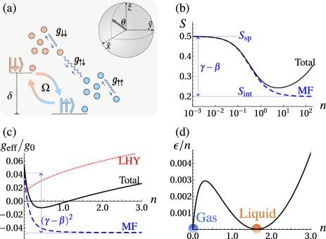
Figure 1: (a) Schematics of a spin twist setup. The spin state of binary bosons, $(\psi_{\uparrow},\psi_{\downarrow})\propto(\cos(\theta/2),\sin(\theta/2))$, can be mapped onto a Bloch sphere with polarization $S\equiv\langle\sigma_{z}\rangle=\cos\theta$. Single-particle potentials $\{\Omega,\ \delta\}$ and spin-dependent interactions $\{g_{\sigma\sigma^{\prime}}\}$ respectively optimize $\theta$ as $\theta_{\rm sp}$ and $\theta_{\rm int}$. A ’spin twist’ occurs when $\theta_{\rm sp}\neq\theta_{\rm int}$ and thus $S_{\rm sp}\neq S_{\rm int}$. (b) Density-tuned polarization from $S_{\rm sp}(=\gamma)$ to $S_{\rm int}(=\beta)$. Dashed and solid lines respectively show mean-field and total (with LHY correction) results. (c) Effective interaction (black solid line) and its individual contribution from mean-field(blue dashed) and LHY(red dot) sectors. The spin twist leads to an additional mean-field repulsion in low-density regime ($\sim(\gamma-\beta)^{2}$), as marked by blue vertical line, which uniquely stabilizes the gas state. (d) Energy per particle (shifted by single-particle energy $-\sqrt{\Omega^{2}+\delta^{2}}$) as a function of density, where the double minima indicate liquid-gas coexistence near their first-order transition. In (b,c,d) we take parameters $(\alpha,\beta,\gamma,\eta)=(-0.1,0.2,0.5,0.0137)$, and scale the density and energy per particle respectively by $\Omega/g_{0}$ and $\Omega$.

In this work, we unveil a new mechanism for the LGTC of ground state bosons (zero $T$) with contact interaction, thereby well beyond the traditional frame as well as previous theorieszero_T_1 ; zero_T_2 . Such mechanism is based on “spin twist”, which refers to a mismatch of spin polarization between single-particle and interaction channels for bosons with spin degrees of freedom. To demonstrate the idea, we consider a concrete setup of binary (pseudo-spin $1/2$) ultracold bosons subject to Rabi coupling ($\Omega$) and magnetic detuning($\delta$), see schematics in Fig.1(a), as explored in previous experimentsLavoine2021:BeyondMeanFieldEffectsRabiCoupled ; Hammond2022:TunableThreeBodyInteractions ; Oberthaler2011 ; Tarruell2022 ; Ferrari . The single-particle potentials ($\Omega,\ \delta$) determine an optimal spin polarization, which can be tuned to mismatch the one determined by spin-dependent interactions (Fig.1(b)). Such spin twist leads to an effective repulsion for low-density bosons (Fig.1(c)), which uniquely stabilizes the gas phase and renders the first-order LGTC in the presence of a quantum droplet at much larger density (Fig.1(d)). In this case, the resulted liquid-gas transition can be conveniently tuned by $\Omega,\ \delta$ and interaction strengths, and moreover, they all occur for thermodynamic systems, in contrast to the finite-size transitions observed previouslyCabrera2018:QuantumLiquidDroplets ; Cheiney2018:BrightSolitonQuantum ; Semeghini2018:SelfBoundQuantumDroplets ; DErrico2019:ObservationQuantumDroplets ; DJWang . To characterize the liquid-gas coexistence, we have pointed out their phase separation in a harmonic trap and further identified two universal exponents for the critical scaling of their densities. Our results can be readily detected in ultracold experiments, and the spin twist scheme can serve as a general tool to engineer LGTC in quantum systems.

Model. We consider the binary bosons ($\uparrow,\downarrow$) with Hamiltonian $H=H_{0}+U$: ($\hbar=1$)

$$H_{0} = \int d{\mathbf{r}}\sum_{\sigma\sigma^{\prime}}\psi_{\sigma}^{\dagger}({\mathbf{r}})\left(-\frac{\nabla^{2}}{2m}\delta_{\sigma\sigma^{\prime}}-[\Omega\sigma_{x}+\delta\sigma_{z}]_{\sigma\sigma^{\prime}}\right)\psi_{\sigma^{\prime}}({\mathbf{r}});$$

$$U = \frac{1}{2}\int d{\mathbf{r}}\sum_{\sigma\sigma^{\prime}}g_{\sigma\sigma^{\prime}}\psi_{\sigma}^{\dagger}({\mathbf{r}})\psi_{\sigma^{\prime}}^{\dagger}({\mathbf{r}})\psi_{\sigma^{\prime}}({\mathbf{r}})\psi_{\sigma}({\mathbf{r}}).$$ (1)

Here $\psi_{\sigma}^{\dagger}(\mathbf{r})$ is the creation operator of spin-$\sigma$, and $\sigma_{i}$ ($i=x,y,z$) are Pauli matrices; $\Omega$ and $\delta$ are respectively the strengths of Rabi coupling and magnetic detuning; $g_{\sigma\sigma^{\prime}}$ is the contact coupling strength between $\sigma$ and $\sigma^{\prime}$, and here we consider $g_{\uparrow\uparrow},g_{\downarrow\downarrow}>0$ and $\delta g\equiv g_{\uparrow\downarrow}+\sqrt{g_{\uparrow\uparrow}g_{\downarrow\downarrow}}<0$, where a stable quantum droplet can be supported in the absence of $\Omega$ and $\delta$Petrov2015:QuantumMechanicalStabilization . The multiple parameters in this problem can be recombined into four dimensionless ones:

$$\alpha\equiv\frac{\delta g}{g_{0}};\ \ \beta\equiv\frac{g_{\downarrow\downarrow}-g_{\uparrow\uparrow}}{4g_{0}};\ \ \gamma\equiv\frac{\delta}{\sqrt{\delta^{2}+\Omega^{2}}};\ \ \eta\equiv m^{3}\Omega g_{0}^{2};$$

with $g_{0}\equiv(g_{\uparrow\uparrow}+g_{\downarrow\downarrow}-2g_{\uparrow\downarrow})/4$. Here $\alpha$ characterizes the strength of overall attractive interaction; $\beta$ and $\gamma$, as shown later, stand for the optimal spin polarizations in interaction and single-particle channels, respectively; $\eta$ measures the Rabi field with respect to interaction strength. To simplify the discussions, in this work we mainly consider the effects of tunable $\alpha$ and $\gamma$.

Spin twist and the induced effective repulsion. Under the mean-field treatment, we replace the field operators by classical numbers: $\psi_{\uparrow}=\sqrt{n}\cos(\theta/2)$, $\psi_{\downarrow}=\sqrt{n}\sin(\theta/2)$, where $n$ is the total density, and $\theta$ determines the spin polarization

$$S\equiv\frac{n_{\uparrow}-n_{\downarrow}}{n_{\uparrow}+n_{\downarrow}}=\cos\theta.$$ (2)

The mean-field energy per volume, $\epsilon_{\rm mf}=E_{\rm mf}/V$, is

$$\epsilon_{\rm mf}=-(\sqrt{1-S^{2}}\Omega+S\delta)n+\frac{g_{0}n^{2}}{2}\left[(S-\beta)^{2}+\frac{g_{\uparrow\uparrow}g_{\downarrow\downarrow}-g_{\uparrow\downarrow}^{2}}{4g_{0}^{2}}\right].$$ (3)

Clearly, the first term contributed from single-particle potentials favors spin polarization $S_{\rm sp}=\gamma$, while the second term from interactions favors $S_{\rm int}=\beta$. A “spin twist” occurs when the two polarizations mismatch, i.e., $\beta\neq\gamma$. The overall mean-field polarization, as determined by $\partial\epsilon_{\rm mf}/\partial S=0$, is shown by dashed line in Fig.1(b), which is density-dependent and can change from $\gamma$ to $\beta$ as $n$ increases.

A remarkable effect of such spin twist is to induce an effective repulsion uniquely in low-density limit. Here we define the effective interaction as

$$g_{\rm eff}\equiv\frac{\partial^{2}\epsilon}{\partial n^{2}},$$ (4)

where $\epsilon$ is the energy density after optimizing $S$. In the absence of spin twist, the two terms in Eq.3 both favor $S=\beta=\gamma$, leading to $g_{\rm eff,mf}^{(0)}=(g_{\uparrow\uparrow}g_{\downarrow\downarrow}-g_{\uparrow\downarrow}^{2})/(4g_{0})$. This is the conventional case of binary bosons, whose mean-field stability is given by $g_{\uparrow\uparrow}g_{\downarrow\downarrow}>g_{\uparrow\downarrow}^{2}$ for any density. However, it is no longer true when spin twist occurs ($\beta\neq\gamma$). In this case, the single-particle and interaction terms compete with each other and the resulted $S$ and $g_{\rm eff,mf}$ are generally $n$-dependent. In the low $n$ limit, the single-particle terms dominate, which result in $S\sim\gamma$ and

$$g_{\rm eff,mf}=g_{\rm eff,mf}^{(0)}+{g_{0}}(\gamma-\beta)^{2}.$$ (5)

Here the spin twist leads to an additional repulsion $\sim{g_{0}}(\gamma-\beta)^{2}$ at the mean-field level. Its physical origin can be understood as follows: since the interactions favor $S\sim\beta$ as ground state, here $S\sim\gamma$ corresponds to an excited spin orientation in the interaction channel, which naturally generate an effective repulsion as above. Note that such repulsion only works for low densities but not high ones, where the interactions dominate and recover $S\sim\beta$ and $g_{\rm eff,mf}\sim g_{\rm eff,mf}^{(0)}$.

Beyond the mean-field treatment, we have further carried out the Bogoliubov analysis and extracted the Lee-Huang-Yang (LHY) energy $\epsilon_{\rm LHY}$ from quantum fluctuationssupple . In Fig.1(c), we plot out the typical $n$-dependent $g_{\rm eff}$ obtained from the total $\epsilon=\epsilon_{\rm mf}+\epsilon_{\rm LHY}$, as well as its individual contributions from mean-field and LHY parts. As expected, the mean-field contribution $g_{\rm eff,mf}$ is positive only in low $n$ limit, and gradually reduces to a negative value as $n$ increases. The reduction is exactly given by $\sim g_{0}(\gamma-\beta)^{2}$ due to spin twist (Eq.5). In comparison, the LHY contribution $g_{\rm eff,LHY}$ is always positive and continuously grows with $n$. The total $g_{\rm eff}$ then displays intriguing sign-changing as $n$ increases: it turns from positive to negative, and back to positive again at large $n$. Consequently, the energy per particle $\epsilon/n$ as a function of $n$ displays double minima, see Fig.1(d). Here the second minimum at finite $n$ is a self-bound droplet with zero pressure that is mainly balanced by mean-field attraction and LHY repulsion, sharing the same spirit as ordinary case Petrov2015:QuantumMechanicalStabilization . While the first minimum at $n=0$, newly found in this work, stands for a gas stabilized by unique low-$n$ repulsion under spin twist (c.f. Eq.5). Such double minima structure implies a first-order transition between liquid and gas as well as their coexistence under proper conditions. We have checked that similar structure cannot appear without spin twistsupple .

From the dressed basis perspective, the gas with $n\sim 0$ and $S\sim\gamma$ essentially occupies the lowest dressed branch as explored in experimentsLavoine2021:BeyondMeanFieldEffectsRabiCoupled ; Hammond2022:TunableThreeBodyInteractions ; Tarruell2022 ; while for the liquid phase at finite $n$, whose polarization can be far from $\gamma$, the single dressed branch is generally not a good description due to considerable population at higher branch.

Ground state phase diagram. The ground state (gas or self-bound droplet) is given by the global minimum in $\epsilon/n(n)$ curve, which is associated with the lowest chemical potential $\mu=\partial\epsilon/\partial n=\epsilon/n$. In Fig.2, we present the ground state phase diagram in $(\alpha,\gamma)$ plane for a given set of $\beta,\eta$. Four phases are shown, i.e., pure droplet (I), droplet with metastable gas (II), gas with metastable droplet (III), and pure gas (IV). Typical $\epsilon/n(n)$ landscapes for different regions are given in the inset plot. The double minima structure appears in regions II and III, and the liquid-gas transition occurs at II-III boundary when they have the same $\epsilon/n=\mu=-\sqrt{\Omega^{2}+\delta^{2}}$, i.e., the single-particle shift.

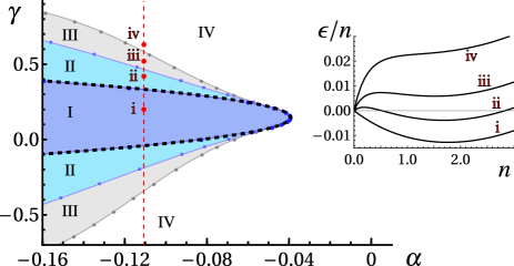
Figure 2: Ground state phase diagram in ($\alpha,\gamma$) plane with fixed $\beta=0.141,\eta=0.0157$. Here I,II,III,IV respectively denote the region where the ground state is a pure droplet, a droplet with metastable gas, a gas with metastable droplet, and a pure gas. The liquid-gas transition occurs at II-III boundary. The inset shows typical $\epsilon/n(n)$ curves for different regions, as marked by ’i,ii,iii,iv’ in the main plot. For each curve $\epsilon/n$ is shifted by single-particle energy ($-\sqrt{\Omega^{2}+\delta^{2}}$). We scale $n$ and $\epsilon/n$ respectively by $\Omega/g_{0}$ and $\Omega$.

We would like to remark a crucial difference between the liquid-gas transition here and those observed previously in binary bosonsCabrera2018:QuantumLiquidDroplets ; Cheiney2018:BrightSolitonQuantum ; Semeghini2018:SelfBoundQuantumDroplets ; DErrico2019:ObservationQuantumDroplets ; DJWang . In previous cases, the transition is driven by the gradually dominant quantum pressure as compared to interaction terms when the boson number $N$ decays, and therefore it occurs for finite-size systems when $N$ reaches a critical value. However, in our case the transition occurs in the thermodynamic limit ($N,V\rightarrow\infty$ with $n=N/V$) and is driven by the competition between single-particle and interaction potentials. Therefore, the current case allows a highly tunable transition point for an arbitrarily large system, and moreover, allows the exploration of liquid-gas coexistence in a considerably broad parameter regime, as shown below.

Liquid-gas coexistence. We now analyze the properties of bosons confined in a harmonic trap. We consider a realistic system of ³⁹K atoms with hyperfine states $|F=1,m_{F}=-1\rangle\equiv|\uparrow\rangle,\ |F=1,m_{F}=0\rangle\equiv|\downarrow\rangle$, as well studied in ultracold droplet experiments(Cabrera2018:QuantumLiquidDroplets, ; Cheiney2018:BrightSolitonQuantum, ; Semeghini2018:SelfBoundQuantumDroplets, ). In this system, $a_{\uparrow\uparrow}=35a_{0},\ a_{\uparrow\downarrow}=-53a_{0}$ ($a_{0}$ is the Bohr radius), and $a_{\downarrow\downarrow}$ is highly tunable by magnetic field. For a concrete demonstration, here we take $a_{\downarrow\downarrow}=64a_{0}$, $\Omega=(2\pi)3.5$kHz (thus $\alpha,\beta,\eta$ are all fixed), and only focus on the coexistence region tuned by $\delta$ (or $\gamma$).

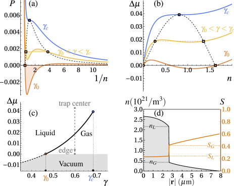
Figure 3: Liquid-gas coexistence(LGC) tuned by $\gamma$ at fixed $\alpha=-0.11,\beta=0.141,\eta=0.0157$. (a) Pressure $P$ as a function of $1/n$ for different $\gamma=0.465(=\gamma_{0}),\ 0.6,\ 0.683(=\gamma_{c})$ (from bottom to top). (b) Shifted chemical potential $\Delta\mu\equiv\mu+\sqrt{\Omega^{2}+\delta^{2}}$ as a function of $n$ for different $\gamma$ as in (a). The intersections between these curves and horizontal lines in (a,b) give the equilibrium densities of liquid ($n_{L}$, squares) and gas ($n_{G}$, circles), which are connected by binodal lines (dashed). For each curve in (a), the two shadow regions have the same area following the Maxwell’s construction. (c) Phase diagram of liquid, gas and vacuum in the ($\gamma,\Delta\mu$) plane. LGC occurs along the black line for $\gamma\in(\gamma_{0},\gamma_{c})$. At $\gamma<\gamma_{0}$, only a self-bound droplet (liquid) is present if $\Delta\mu$ is above the dashed line. At $\gamma>\gamma_{c}$, the liquid and gas are indistinguishable. (d) Profiles of total density($n$) and spin polarization($S$) for bosons in an isotropic harmonic trap with frequency $\omega=(2\pi)50$Hz, total number $N=4\times 10^{5}$ and $\gamma=0.6$, corresponding to the vertical trajectory shown in (c). The sharp jumps of $n$ and $S$ mark the location of LGC. For all plots, we scale the density and energy per particle respectively by $\Omega/g_{0}$ and $\Omega$.

The coexistence of liquid and gas requires

$$\mu(n_{L})=\mu(n_{G}),\ \ \ \ \ \ P(n_{L})=P(n_{G});$$ (6)

where $n_{L}\ (n_{G})$ is the liquid (gas) density at equilibrium, $\mu$ is the chemical potential and $P=\mu n-\epsilon$ is the pressure. In Fig.3(a,b), we plot out $P(1/n)$ and $\mu(n)$ for several typical $\gamma$. We can see that $P(1/n)$ shows similar lineshape as classical $P$-$V$ isotherms hosting LGTCLandau_Lifshitz ; Huang1991:StatisticalMechanics2nd . Here we have used the Maxwell’s construction to identify $n_{L}$ and $n_{G}$, as marked respectively by squares and circles in Fig.3(a). Specifically, $n_{L}$ ($n_{G}$) is given by the left (right) intersection between each $P(1/n)$ curve and a horizontal line, by requiring the same area of two separated shadow regions. The relation $\int d\mu=\int 1/ndP$ then guarantees the same $\mu$ at the intersections (see also Fig.3(b)), which will be denoted as $\mu_{\rm LGC}$ from now on.

Fig.3(a,b) also indicate a finite parameter window, $\gamma\in(\gamma_{0},\gamma_{c})$, for the occurrence of liquid-gas coexistence. At the lower bound $\gamma_{0}$, a gas phase starts to emerge at $n_{G}=0$ and the two phases have $\mu=-\sqrt{\Omega^{2}+\delta^{2}}$ and $P=0$. This is right at the ground state transition between liquid and gas, i.e., at the II-III boundary shown in Fig.2. As increasing $\gamma$, the coexisting phases has higher $\mu,\ P$ and meanwhile $n_{G}$ and $n_{L}$ get closer. Finally the coexistence terminates at the critical point $\gamma_{c}$ when $n_{L},\ n_{G}$ merge into a single value($n_{c}$) at the inflections of $\mu(n)$ and $P(1/n)$ curves. For even larger $\gamma>\gamma_{c}$, the gas and liquid become indistinguishable.

Fig.3(c) further summarizes the results in $(\gamma,\mu)$ plane, where $\mu_{\rm LGC}$ (solid line) separates the liquid and gas for $\gamma\in(\gamma_{0},\gamma_{c})$. To observe their coexistence, we suggest measuring the density profiles of bosons under an external trap, and here for brevity we consider an isotropic harmonic trap $V({\mathbf{r}})=m\omega^{2}{\bf r}^{2}/2$. Using the local density approximation $\mu({\mathbf{r}})=\mu(0)-V({\mathbf{r}})$, in Fig.3(d) we plot out the typical profiles of $n$ and $S$ in the trap showing liquid-gas phase separation, where liquid and gas respectively occupy the trap center and edge. At their interface $n$ ($S$) displays sharp jump from $n_{L}$ to $n_{G}$ ($S_{L}$ to $S_{G}$), marking the location of liquid-gas coexistence with $\mu=\mu_{\rm LGC}$. Note that $n_{L,G}$ and $S_{L,G}$ do not depend on specific boson number $N$, as long as it is above a critical valuesupple .

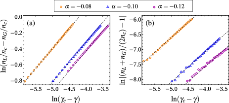
Figure 4: Universal critical scaling for the relative (a) and averaged (b) densities of liquid and gas at their coexistence. $\beta,\eta$ are the same as in Fig.3. Discrete points show numerical data and dashed lines show linear fittings. Here we take $\ln$-$\ln$ plot, and the slopes for all fitting lines in (a) are $1/2$ and in (b) are $1$, giving the according exponents $\lambda$ and $\xi$ defined in Eq.(7).

Interestingly, the liquid and gas obey universal critical scaling near the melting of LGTC. Here we explore the asymptotic behavior of their relative and mean densities near $\gamma\sim\gamma_{c}$ and $n_{L}\sim n_{G}\sim n_{c}$:

$$\frac{n_{L}-n_{G}}{n_{c}}\propto(\gamma_{c}-\gamma)^{\lambda};\ \ \ \frac{n_{L}+n_{G}}{2n_{c}}-1\propto(\gamma_{c}-\gamma)^{\xi},$$ (7)

with $\lambda,\ \xi$ the according critical exponents. In Fig.4(a,b), we have numerically extracted the exponents as $\lambda=1/2$ and $\xi=1$ for all given $\alpha$. These exponents also universally persist for other tunable parameters, such as changing $\gamma$ to $\alpha$supple . To explain such universal phenomenon, we have adopted a mean-field theory as in the classical treatment of finite $T$ liquid-gas transitionChaikin1995:PrinciplesCondensedMatter , which well predicts the universal critical exponents as abovesupple .

Here we clarify that the liquid-gas coexistence here should be distinguished from the equilibrium of a droplet and a fully polarized gas in previous studiesLGC1 ; LGC2 ; LGC3 ; LGC4 , where $\Omega,\delta$ are both absent. The latter is due to a preset spin population that deviates from the one preferred by droplet, and therefore the residue (single-species) bosons are repelled out of the droplet to form gas. In contrast, the coexistence here is associated with first-order liquid-gas transition (Fig.1), where the spin population is changeable and both species can transfer freely between two phases to reach mutual equilibration.

Summary. We have revealed a new mechanism using spin twist to engineer liquid-gas transition and coexistence (LGTC) in ground state bosons, which does not rely on thermal effect or long-range potential. The scheme is demonstrated with a specific model of binary bosons under Rabi coupling and magnetic detuning. Take the realistic ³⁹K atoms for example, in practice one can follow the strategy in Lavoine2021:BeyondMeanFieldEffectsRabiCoupled ; Hammond2022:TunableThreeBodyInteractions ; Tarruell2022 to prepare a gas at ground state, from which a liquid (droplet) can be approached by changing $\gamma$ or $\alpha$ following Fig.2. The LGTC naturally occur during this process, and the proposed phase separation in a trap and universal scaling of equilibrium densities can be readily tested in experiments.

Finally, we remark that the spin twist in creating an effective low-density repulsion for gas stabilization is a very robust mechanism, which can be applied to a wide class of quantum systems with competing single-particle and interaction orders. For instance, it is expected to still work when add more spin degrees of freedom, or change $\Omega,\delta$ to other single-particle potentials in altering spins. In this regard, the spin twist can serve as a general principle for achieving LGTC at ultra-low temperatures, which hopefully would promote the practical use of such phenomena in a fascinating quantum world in future.

Supplementary Materials

This supplemental file includes the derivations of beyond-mean-field correction, details on liquid-gas coexistence in trapped system, and theoretical explanation of universal scaling near the critical point.

I Beyond-mean-field correction

I.1 The Bogoliubov method and LHY correction

The Hamiltonian in the momentum space is $H=H_{0}+U$, where

$$H_{0} =\sum_{\mathbf{k}}\left[\epsilon^{0}_{\mathbf{k}}(\psi^{\dagger}_{\uparrow,\mathbf{k}}\psi_{\uparrow,\mathbf{k}}+\psi^{\dagger}_{\downarrow,\mathbf{k}}\psi_{\downarrow,\mathbf{k}})-{\Omega}(\psi^{\dagger}_{\uparrow,\mathbf{k}}\psi_{\downarrow,\mathbf{k}}+\psi^{\dagger}_{\downarrow,\mathbf{k}}\psi_{\uparrow,\mathbf{k}})-{\delta}(\psi^{\dagger}_{\uparrow,\mathbf{k}}\psi_{\uparrow,\mathbf{k}}-\psi^{\dagger}_{\downarrow,\mathbf{k}}\psi_{\downarrow,\mathbf{k}})\right];$$ (S1)

$$U =\frac{1}{2V}\sum_{\mathbf{q,p,k}}\sum_{\sigma\sigma^{\prime}}\left[g_{\sigma\sigma^{\prime}}\psi^{\dagger}_{\sigma,\mathbf{q+k}}\psi^{\dagger}_{\sigma^{\prime},\mathbf{q-k}}\psi_{\sigma^{\prime},\mathbf{q+p}}\psi_{\sigma,\mathbf{q-p}}\right]$$

According to the standard Bogoliubov method, we have the quadratic Hamiltonian

$$\frac{H}{V}=\frac{E_{\text{mf}}}{V}+\frac{1}{2V}\sum_{\sigma\sigma^{\prime}}g^{2}_{\sigma\sigma^{\prime}}n_{\sigma}n_{\sigma^{\prime}}\sum_{\mathbf{k}\neq 0}\frac{1}{2\epsilon^{0}_{\mathbf{k}}}-\frac{1}{2V}\sum_{\mathbf{k}\neq 0}\Big{(}2\epsilon^{0}_{\mathbf{k}}+{\Omega}\frac{(n_{\uparrow}+n_{\downarrow})}{\sqrt{n_{\uparrow}n_{\downarrow}}}+g_{\upuparrows}n_{\uparrow}+g_{\downdownarrows}n_{\downarrow}\Big{)}+\frac{1}{2V}\sum_{\mathbf{k}\neq 0}A^{\dagger}H_{\text{Bog}}A,$$ (S2)

where $A^{\dagger}=(\psi^{\dagger}_{\uparrow,\mathbf{k}},\psi_{\uparrow,-\mathbf{k}},\psi^{\dagger}_{\downarrow,\mathbf{k}},\psi_{\downarrow,-\mathbf{k}})$, and

$$H_{\text{Bog}}=\begin{pmatrix}\epsilon^{0}_{\mathbf{k}}+{\Omega}\sqrt{\frac{n_{\downarrow}}{n_{\uparrow}}}+g_{\upuparrows}n_{\uparrow}&g_{\upuparrows}n_{\uparrow}&g_{\uparrow\!\downarrow}\sqrt{n_{\uparrow}n_{\downarrow}}-{\Omega}&g_{\uparrow\!\downarrow}\sqrt{n_{\uparrow}n_{\downarrow}}\\ g_{\upuparrows}n_{\uparrow}&\epsilon^{0}_{\mathbf{k}}+{\Omega}\sqrt{\frac{n_{\downarrow}}{n_{\uparrow}}}+g_{\upuparrows}n_{\uparrow}&g_{\uparrow\!\downarrow}\sqrt{n_{\uparrow}n_{\downarrow}}&g_{\uparrow\!\downarrow}\sqrt{n_{\uparrow}n_{\downarrow}}-{\Omega}\\ g_{\uparrow\!\downarrow}\sqrt{n_{\uparrow}n_{\downarrow}}-{\Omega}&g_{\uparrow\!\downarrow}\sqrt{n_{\uparrow}n_{\downarrow}}&\epsilon^{0}_{\mathbf{k}}+{\Omega}\sqrt{\frac{n_{\uparrow}}{n_{\downarrow}}}+g_{\downdownarrows}n_{\downarrow}&g_{\downdownarrows}n_{\downarrow}\\ g_{\uparrow\!\downarrow}\sqrt{n_{\uparrow}n_{\downarrow}}&g_{\uparrow\!\downarrow}\sqrt{n_{\uparrow}n_{\downarrow}}-{\Omega}&g_{\downdownarrows}n_{\downarrow}&\epsilon^{0}_{\mathbf{k}}+{\Omega}\sqrt{\frac{n_{\uparrow}}{n_{\downarrow}}}+g_{\downdownarrows}n_{\downarrow}\end{pmatrix}.$$ (S3)

Under the Bogoliubov transformation, $H_{\text{Bog}}$ is diagonal in the basis of quasi-particle operators $\{b_{\pm,\mathbf{k}}\}$,

$$\dfrac{1}{2}A^{\dagger}H_{\text{Bog}}A=\frac{1}{2}\mathcal{E}_{+,\mathbf{k}}\Big{(}b^{\dagger}_{+,\mathbf{k}}b_{+,\mathbf{k}}+b_{+,-\mathbf{k}}b^{\dagger}_{+,-\mathbf{k}}\Big{)}+\frac{1}{2}\mathcal{E}_{-,\mathbf{k}}\Big{(}b^{\dagger}_{-,\mathbf{k}}b_{-,\mathbf{k}}+b_{-,-\mathbf{k}}b^{\dagger}_{-,-\mathbf{k}}\Big{)}.$$ (S4)

The Bogoliubov modes $\mathcal{E}_{\pm}$ satisfy

$$\bigg{\|}H_{\text{Bog}}-\mathcal{E}\begin{pmatrix}\sigma_{z}&0\\ 0&\sigma_{z}\end{pmatrix}\bigg{\|}=0.$$ (S5)

This gives

$$\mathcal{E}_{\{\pm\},\mathbf{k}}=\sqrt{D_{\mathbf{k}}\pm\sqrt{D_{\mathbf{k}}^{2}-\epsilon^{0}_{\mathbf{k}}\Big{(}\epsilon^{0}_{\mathbf{k}}+{\Omega}\frac{n_{\uparrow}+n_{\downarrow}}{\sqrt{n_{\uparrow}n_{\downarrow}}}\Big{)}\Big{[}\big{(}\epsilon^{0}_{\mathbf{k}}+2g_{\upuparrows}n_{\uparrow}+{\Omega}\sqrt{\frac{n_{\downarrow}}{n_{\uparrow}}}\big{)}\big{(}\epsilon^{0}_{\mathbf{k}}+2g_{\downdownarrows}n_{\downarrow}+{\Omega}\sqrt{\frac{n_{\uparrow}}{n_{\downarrow}}}\big{)}-\big{(}2g_{\uparrow\!\downarrow}\sqrt{n_{\uparrow}n_{\downarrow}}-{\Omega}\big{)}^{2}\Big{]}}}$$ (S6)

with

$$D_{\mathbf{k}}=\frac{1}{2}\Big{(}\epsilon^{0}_{\mathbf{k}}+g_{\upuparrows}n_{\uparrow}+{\Omega}\sqrt{\frac{n_{\downarrow}}{n_{\uparrow}}}\Big{)}^{2}+\frac{1}{2}\Big{(}\epsilon^{0}_{\mathbf{k}}+g_{\downdownarrows}n_{\downarrow}+{\Omega}\sqrt{\frac{n_{\uparrow}}{n_{\downarrow}}}\Big{)}^{2}+\Big{(}g_{\uparrow\!\downarrow}\sqrt{n_{\uparrow}n_{\downarrow}}-{\Omega}\Big{)}^{2}-\frac{1}{2}\sum_{\sigma\sigma^{\prime}}g_{\sigma\sigma^{\prime}}^{2}n_{\sigma}n_{\sigma^{\prime}}.$$ (S7)

The total energy density that includes the quantum fluctuation can be obtained from Eq.(S2) and (S4) as

$$\frac{E}{V}=\frac{E_{\text{mf}}}{V}+\frac{1}{2V}\sum_{\mathbf{k}\neq 0}\bigg{(}\sum_{\sigma\sigma^{\prime}}g^{2}_{\sigma\sigma^{\prime}}n_{\sigma}n_{\sigma^{\prime}}\frac{1}{2\epsilon^{0}_{\mathbf{k}}}-\Big{(}2\epsilon^{0}_{\mathbf{k}}+{\Omega}\frac{(n_{\uparrow}+n_{\downarrow})}{\sqrt{n_{\uparrow}n_{\downarrow}}}+g_{\upuparrows}n_{\uparrow}+g_{\downdownarrows}n_{\downarrow}\Big{)}+\mathcal{E}_{+,\mathbf{k}}+\mathcal{E}_{-,\mathbf{k}}\bigg{)}$$ (S8)

In the large k limit, $\mathcal{E}_{\pm,\bf k}$ has the form $\sqrt{{\epsilon^{0}_{\bf k}}^{2}+c{\epsilon^{0}_{\bf k}}+c_{0}\pm\sqrt{c_{1}{\epsilon^{0}_{\bf k}}^{2}+c_{2}{\epsilon^{0}_{\bf k}+c_{3}}}}$, where $c,c_{0},c_{1},c_{2}$, and $c_{3}$ are lengthy expressions extracted from Eq.(S6), e.g., $c=g_{\upuparrows}n_{\uparrow}+g_{\downdownarrows}n_{\downarrow}+\Omega\frac{(n_{\uparrow}+n_{\downarrow})}{\sqrt{n_{\uparrow}n_{\downarrow}}}$, $c_{0}=(g_{\upuparrows}+g_{\downdownarrows}-2g_{\uparrow\!\downarrow})\Omega\sqrt{n_{\uparrow}n_{\downarrow}}+\frac{(n_{\uparrow}+n_{\downarrow})^{2}\Omega^{2}}{2n_{\uparrow}n_{\downarrow}}$, and $c_{1}=4c_{0}-c^{2}+2\sum_{\sigma\sigma^{\prime}}g^{2}_{\sigma\sigma^{\prime}}n_{\sigma}n_{\sigma^{\prime}}$. Then we have $\mathcal{E}_{+,\bf k}+\mathcal{E}_{-,\bf k}\sim 2\epsilon^{0}_{\bf k}+c+(c_{0}-\frac{c^{2}}{4}-\frac{c_{1}}{4})\frac{1}{\epsilon^{0}_{\bf k}}+O(\frac{1}{{\epsilon^{0}_{\bf k}}^{2}})$, and therefore the ultraviolet divergence for the integration of various terms in Eq.(S8) can be exactly cancelled.

Given $E(n_{\uparrow},n_{\downarrow})=E(n,S)$ (here $S=\cos\theta$ is the spin polarization), one can find the optimal spin polarization via ${\partial E(n,S)}/{\partial S}=0$. In practice, we set $\delta g=0$ in numerically calculating quantum fluctuations in order to avoid the complex excitation spectra at small k. In fact, for $\delta g<0$ the imaginary excitation spectra can be rectified by considering the high-order fluctuations, and such high-order terms turn out to only produce little modification to the total fluctuation energy as long as $|\delta g|\ll|g_{ij}|$ [1].

I.2 Effective two-body interaction at low-density limit

In the low $n$ limit, the optimal spin polarization is given by the single-particle configuration, $\cos\theta=S_{\text{sp}}=\gamma$. Here we have the single-particle eigen-states:

$$\begin{pmatrix}\ket{-}\\ \ket{+}\end{pmatrix}=\begin{pmatrix}\cos\frac{\theta}{2}&\sin\frac{\theta}{2}\\ -\sin\frac{\theta}{2}&\cos\frac{\theta}{2}\end{pmatrix}\begin{pmatrix}\ket{\uparrow}\\ \ket{\downarrow}\end{pmatrix},$$ (S9)

and in such $\{+,-\}$ basis the original Hamiltonian (S1) can be translated into

$$H = \sum_{\bf k}\left[\left(\epsilon^{0}_{\bf k}-\sqrt{\Omega^{2}+\delta^{2}}\right)\psi_{-,\bf k}^{\dagger}\psi_{-,\bf k}+\left(\epsilon^{0}_{\bf k}+\sqrt{\Omega^{2}+\delta^{2}}\right)\psi_{+,\bf k}^{\dagger}\psi_{+,\bf k}\right]+\frac{1}{2V}\tilde{\sum}_{\bf\{k_{i}\}}\big{\{}\ g_{1}\psi_{-,\bf k_{1}}^{\dagger}\psi_{-,\bf k_{2}}^{\dagger}\psi_{-,\bf k_{3}}\psi_{-,\bf k_{4}}$$

$$+g_{2}\psi_{+,\bf k_{1}}^{\dagger}\psi_{+,\bf k_{2}}^{\dagger}\psi_{+,\bf k_{3}}\psi_{+,\bf k_{4}}+g_{3}(\psi_{-,\bf k_{1}}^{\dagger}\psi_{+,\bf k_{2}}^{\dagger}\psi_{+,\bf k_{3}}\psi_{-,\bf k_{4}}+{\rm h.c})+g_{4}(\psi_{-,\bf k_{1}}^{\dagger}\psi_{+,\bf k_{2}}^{\dagger}\psi_{-,\bf k_{3}}\psi_{+,\bf k_{4}}+{\rm h.c})$$

$$+g_{5}(\psi_{-,\bf k_{1}}^{\dagger}\psi_{-,\bf k_{2}}^{\dagger}\psi_{+,\bf k_{3}}\psi_{+,\bf k_{4}}+{\rm h.c.})+g_{6}(\psi_{-,\bf k_{1}}^{\dagger}\psi_{-,\bf k_{2}}^{\dagger}\psi_{-,\bf k_{3}}\psi_{+,\bf k_{4}}+{\rm h.c.})+g_{7}(\psi_{+,\bf k_{1}}^{\dagger}\psi_{+,\bf k_{2}}^{\dagger}\psi_{+,\bf k_{3}}\psi_{-,\bf k_{4}}+{\rm h.c.})\big{\}},$$

where $\tilde{\sum}_{\bf\{k_{i}\}}$ includes momentum conservation. The effective two-body interaction under the second-order perturbation is

$$g_{\text{eff}}^{(2)}=\leavevmode\hbox to4pt{\vbox to4pt{\text{[drawing]}}}+\leavevmode\hbox to4pt{\vbox to4pt{\text{[drawing]}}}+\leavevmode\hbox to4pt{\vbox to4pt{\text{[drawing]}}}+\leavevmode\hbox to4pt{\vbox to4pt{\text{[drawing]}}}, (v1)+(-0.4cm,+0.4cm) (v1)+(-0.4cm,-0.4cm) (v1)+(+0.4cm,+0.4cm) (v1)+(+0.4cm,-0.4cm) - - - - (v1)+(-0.4cm,+0.4cm) (v1)+(-0.4cm,-0.4cm) (v2)+(+0.4cm,+0.4cm) (v2)+(+0.4cm,-0.4cm) - -\ \ \ \ - - - -\ \ \ \ - - (v1)+(-0.4cm,+0.4cm) (v1)+(-0.4cm,-0.4cm) (v2)+(+0.4cm,+0.4cm) (v2)+(+0.4cm,-0.4cm) - +\ \ \ \ + - - +\ \ \ \ + - (v1)+(-0.4cm,+0.4cm) (v1)+(-0.4cm,-0.4cm) (v2)+(+0.4cm,+0.4cm) (v2)+(+0.4cm,-0.4cm) - +\ \ \ \ + - - -\ \ \ \ - - (v1)+(-0.4cm,+0.4cm) (v1)+(-0.4cm,-0.4cm) (v1)+(+0.4cm,+0.4cm) (v1)+(+0.4cm,-0.4cm) - - - - (v1)+(-0.4cm,+0.4cm) (v1)+(-0.4cm,-0.4cm) (v2)+(+0.4cm,+0.4cm) (v2)+(+0.4cm,-0.4cm) - -\ \ \ \ - - - -\ \ \ \ - - (v1)+(-0.4cm,+0.4cm) (v1)+(-0.4cm,-0.4cm) (v2)+(+0.4cm,+0.4cm) (v2)+(+0.4cm,-0.4cm) - +\ \ \ \ + - - +\ \ \ \ + - (v1)+(-0.4cm,+0.4cm) (v1)+(-0.4cm,-0.4cm) (v2)+(+0.4cm,+0.4cm) (v2)+(+0.4cm,-0.4cm) - +\ \ \ \ + - - -\ \ \ \ - -$$ (S11)

where the vertices are $\leavevmode\hbox to4pt{\vbox to4pt{\text{[drawing]}}}\equiv g_{1}=g_{\text{eff,mf}},\quad\leavevmode\hbox to4pt{\vbox to4pt{\text{[drawing]}}}\equiv g_{5}=g_{0}\sin^{2}{\theta},\quad\text{and}\quad\leavevmode\hbox to4pt{\vbox to4pt{\text{[drawing]}}}\equiv{g_{6}}/{\sqrt{2}}=\sqrt{2}\sin\!\theta(\cos\!\theta-\beta)g_{0}.$ The internal lines refer to the single-particle Green’s functions:

$$G^{0}_{--}(p)={1}/{(p^{0}-\epsilon_{p}^{0}+i0^{+})}\ \ \text{and}\ \ \ G^{0}_{++}(p)={1}/{(p^{0}-\epsilon_{p}^{0}-{2\sqrt{\Omega^{2}+\delta^{2}}}+i0^{+})}.$$ (S12)

With the renormalization relations $g_{\sigma\sigma^{\prime}}\to g_{\sigma\sigma^{\prime}}+g_{\sigma\sigma^{\prime}}^{2}\int\frac{1}{2\epsilon^{0}_{k}}\frac{d^{3}k}{(2\pi)^{3}}$ and the fact $\sum_{\sigma\sigma^{\prime}}g_{\sigma\sigma^{\prime}}^{2}n_{\sigma}n_{\sigma^{\prime}}/n^{2}=g_{1}^{2}+g_{5}^{2}+g_{6}^{2}/2$, we can straightforwardly perform

$$g_{\text{eff}}^{(2)} =g_{\text{eff,mf}}+g_{1}^{2}\int\!\frac{d^{3}k}{(2\pi)^{3}}\left(i\!\int\!\frac{dk^{0}}{2\pi}G^{0}_{--}(k)G^{0}_{--}(-k)+\frac{1}{2\epsilon^{0}_{k}}\right)$$ (S13)

$$\ \ \ +g_{5}^{2}\int\!\frac{d^{3}k}{(2\pi)^{3}}\left(i\!\int\!\frac{dk^{0}}{2\pi}G^{0}_{++}(k)G^{0}_{++}(-k)+\frac{1}{2\epsilon^{0}_{k}}\right)+\frac{g_{6}^{2}}{2}\int\!\frac{d^{3}k}{(2\pi)^{3}}\left(i\!\int\!\frac{dk^{0}}{2\pi}G^{0}_{++}(k)G^{0}_{--}(-k)+\frac{1}{2\epsilon^{0}_{k}}\right),$$

and obtain the effective interaction

$$g_{\text{eff}}^{(2)}=g_{\text{eff,mf}}+\frac{(1-\gamma^{2})^{3/4}}{2\pi}\left[1-\gamma^{2}+\sqrt{2}(\gamma-\beta)^{2}\right]\eta^{1/2}g_{0}.$$ (S14)

Note that $g_{\text{eff}}^{(2)}$ above is exactly the effective interaction for the lowest dressed branch of the single-particle states. It is composed by two parts: $g_{\text{eff,mf}}$ is the mean-field contribution, and the second part is contributed from the quantum fluctuations (or Lee-Huang-Yang(LHY) corrections), as shown by the red dot line in Fig.1(c) and Fig.S1 at $n\rightarrow 0$. In the special case $\beta=\gamma$, this part reproduces the LHY-induced two-body interaction as discussed in Ref.[2]. Here the existence of (meta)stable gas requires $g_{\text{eff}}^{(2)}>0$, and the boundary $g_{\text{eff}}^{(2)}=0$ is shown as the black dashed line in Fig.2 (separating regions I and II).

I.3 Spin twist and double minima structure

To demonstrate the vital role of spin twist played in the liquid-gas coexistence, in Fig.S1 we compare the $\epsilon/n(n)$ curves with and without spin twist. Fig.S1(a,b,c) are for the case with spin twist ($\beta\neq\gamma$), which are identical to Fig.1(b,c,d) in the main text. It shows that the spin twist can result in an additional mean-field repulsion in the low-$n$ regime, which uniquely stabilizes the gas state and facilitates the liquid-gas coexistence in view of the double minima structure of $\epsilon/n(n)$ curve. In comparison, Fig.S1(d,e,f) are for the case without spin twist ($\beta=\gamma$), where the mean-field contributions to $S$ and $g_{\rm eff}$ are both static for all densities and the resulted $\epsilon/n(n)$ can only show one minimum (representing either liquid or gas) but not two. In the latter case, the liquid and gas cannot be (locally) stable simultaneously and thus cannot coexist.

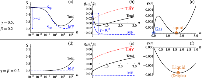
Fig. S1: The polarization, effective interaction and energy per particle curves, with (upper panel) and without (lower panel) spin-twist. The case of spin twist is identical to that shown in Fig.1(b,c,d). Without spin-twist, the total effective interaction $g_{\rm eff}$ always increases monotonically, and the energy per particle $\epsilon/n$ presents only one minimum, namely gas or droplet state. $\alpha$ and $\eta$ are the same as in Fig.1.

II Liquid-gas coexistence in a harmonic trap

Here we present more details on the coexistence of liquid and gas in an isotropic harmonic trap $V({\mathbf{r}})$, as shown by Fig.3 in the main text.

At the coexistence of liquid and gas, let us denote $\mu(n_{L})=\mu(n_{G})\equiv\mu_{\rm LGC}$. Then according to the $P(1/n)$ and $\mu(n)$ curves in Fig.3(a,b), we can see that the gas phase stays for $\mu<\mu_{\rm LGC}$, as it has a higher pressure (and thus a lower thermodynamic potential) than liquid; while the liquid phase stays for $\mu>\mu_{\rm LGC}$, at it has a higher pressure than gas. In Fig.S2(a), we show the occupation of gas and liquid in the $\mu$-$n$ plane taking a typical value of $\gamma\in(\gamma_{0},\gamma_{c})$.

Under the local density approximation $\mu({\mathbf{r}})=\mu(0)-V({\mathbf{r}})$, the local $\mu$ decays from the trap center to edge. Then it follows that the liquid phase with higher $\mu(>\mu_{\rm LGC})$ locates at the trap center, and the gas phase with lower $\mu(<\mu_{\rm LGC})$ locates at the edge. To enable the coexistence of liquid and gas in the trap, the chemical potential $\mu(0)$ at the trap center should be higher than $\mu_{\rm LGC}$, which requires the boson number $N$ be larger than a critical value $N_{c}$. In other words, at $N=N_{c}$, $\mu(0)$ reaches $\mu_{\rm LGC}$ and a liquid phase starts to emerge at the trap center. In Fig.S2(b), we plot out $N_{c}$ as a function of $\gamma$ (solid line). The liquid-gas coexistence occurs within $\gamma\in(\gamma_{0},\gamma_{c})$ once $N>N_{c}$, as shown by the colored region therein.

As shown by Fig.3(d) in the main text, at the liquid-gas interface the total density $n$ undergoes a discontinuous jump from $n_{L}$ to $n_{G}$, and the spin polarization $S$ jumps from $S_{L}$ to $S_{G}$. Here we emphasize that such discontinuities are universal for different $N(>N_{c})$. As shown by Fig.S2(c1,c2), different $N$ would not alter $n_{L,G}$ and $S_{L,G}$ at the liquid-gas interface, but just change the size of liquid phase in the trap. Therefore $n_{L,G}$ and $S_{L,G}$ can serve as universal quantities to characterize the liquid-gas coexistence for thermodynamic systems.

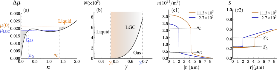
Fig. S2: Liquid-gas coexistence at fixed $\alpha=-0.11,\beta=0.141,\eta=0.0157$. (a) Shifted chemical potential $\Delta\mu\equiv\mu+\sqrt{\Omega^{2}+\delta^{2}}$ as a function of $n$ at $\gamma=0.6$. The blue horizontal line marks the shifted $\mu_{\rm LGC}$ at liquid-gas coexistence, and the orange horizontal line marks the shifted chemical potential $\mu(0)$ at trap center. The gas (liquid) state populates $\mu<\mu_{\rm LGC}$ ($\mu>\mu_{\rm LGC}$). (b) Phases tuned by $\gamma$ and boson number $N$ in an isotropic harmonic trap with frequency $\omega=(2\pi)50$Hz. The coexistence occurs in the colored region with $N>N_{c}$ and $\mu(0)>\mu_{\rm LGC}$. (c1,c2): Profiles of total density $n$ and spin polarization $S$ for different boson numbers $N$ at fixed $\gamma=0.6$. At the liquid-gas interface $n_{L,G}$ and $S_{L,G}$ are universal values for all $N(>N_{c})$. For all plots, we scale the density and energy per particle respectively by $\Omega/g_{0}$ and $\Omega$.

III Critical exponents near the melting of liquid-gas coexistence

Inspired by the classical treatment of temperature-driven liquid-gas coexistence in Ref.[3], here we introduce the mixed thermodynamic function $W(x,\mu,n)=\epsilon(x,\mu,n)-\mu n$, which determines the equilibrium state via $\partial W/\partial n=0$ and the coexistence critical point via $\partial^{2}W(x_{c},\mu_{c},n_{c})/\partial n^{2}=\partial^{3}W(x_{c},\mu_{c},n_{c})/\partial n^{3}=0$. The variable $x$ here can represent any tunable parameter we are interested in, such as $\gamma$ or $\alpha$ in this work.

We expand $W(x,\mu,n)$ near the critical point to the fourth-order of $(n-n_{c})$:

$$W(x,\mu,n)=W(x,\mu,n_{c})+\sum_{i=1}^{i=4}w_{i}(n-n_{c})^{i},$$ (S15)

where $w_{4}(x,\mu,n_{c})$ is finite, and $w_{1,2,3}(x,\mu,n_{c})$ is close to zero and can be expanded in terms of $(x-x_{c})$ and $(\mu-\mu_{c})$,

$$w_{1}=\frac{\partial W(x,\mu,n_{c})}{\partial n}=\frac{\partial^{2}\epsilon(x_{c},n_{c})}{\partial n\partial x}(x-x_{c})-(\mu-\mu_{c}),\quad w_{\{i=2,3\}}=\frac{\partial^{i}W(x,\mu,n_{c})}{i!\ \partial n^{i}}=\frac{\partial^{i+1}\epsilon(x_{c},n_{c})}{i!\ \partial n^{i}\partial x}(x-x_{c}).$$ (S16)

Denoting $\phi=(n_{L}-n_{G})/2$ and $\phi_{0}=(n_{L}+n_{G})/2-n_{c}$, we have

$$n_{L}-n_{c}=\phi_{0}+\phi\quad\text{and}\quad n_{G}-n_{c}=\phi_{0}-\phi.$$ (S17)

Substituting Eq.(S17) into Eq.(S15), and rearranging the expansion in terms of $\phi^{i}$, we have

$$W(x,\mu,n_{L}) =W(x,\mu,n_{c})+\sum_{i=1}^{i=4}\left(w_{i}\phi_{0}^{i}+\tilde{w}_{i}\phi^{i}\right),$$ (S18)

$$W(x,\mu,n_{G}) =W(x,\mu,n_{c})+\sum_{i=1}^{i=4}\left(w_{i}\phi_{0}^{i}+(-1)^{i}\tilde{w}_{i}\phi^{i}\right),$$

where the coefficients are

$$\tilde{w}_{1} =w_{1}+2w_{2}\phi_{0}+3w_{3}\phi_{0}^{2}+4w_{4}\phi_{0}^{3},$$ (S19)

$$\tilde{w}_{2} =w_{2}+3w_{3}\phi_{0}+6w_{4}\phi_{0}^{2},$$

$$\tilde{w}_{3} =w_{3}+4w_{4}\phi_{0},$$

$$\tilde{w}_{4} =w_{4}.$$

At coexistence, $n_{L}$ and $n_{G}$ share the same pressure $P(n_{L})=P(n_{G})\equiv-W(x,\mu,n)_{\rm min}$. This mean that for Eq.(S18) with a given $\phi_{0}$, we have $W(x,\mu,n_{L})=W(x,\mu,n_{G})$. Therefore, the terms of the odd-order of $\phi$ are absent in Eq.(S18), i.e., $\tilde{w}_{1}=\tilde{w}_{3}=0$, which leads to

$$\phi_{0}=\frac{-w_{3}}{4w_{4}}=\frac{-1}{4w_{4}}\frac{\partial^{4}\epsilon(x_{c},n_{c})}{\partial n^{3}\partial x}(x-x_{c}).$$ (S20)

The function $W(x,\mu,n)$ in Eq.(S18) is then reduced to $W_{0}(x,\mu,\phi_{0})+\tilde{w}_{2}\phi^{2}+w_{4}\phi^{4}$, whose minimum describes the equilibrium state with

$$\phi^{2}=\frac{-\tilde{w}_{2}}{2w_{4}}=\frac{-1}{2w_{4}}\frac{\partial^{3}\epsilon(x_{c},n_{c})}{\partial n^{2}\partial x}(x-x_{c})+O\left((x-x_{c})^{2}\right).$$ (S21)

Eq.(S20) and (S21) give the critical exponents $\xi=1$ and $\lambda=1/2$.

Note that above derivation applies to any tunable parameter $x$. In the main text we have chosen $x=\gamma$, while keeping other parameters fixed. In Fig.S3, we choose $x=\alpha$ as the tunable parameter, and find that the two critical exponents $\xi=1$ and $\lambda=1/2$ still apply in this case. Therefore, these exponents are universal ones in characterizing the liquid-gas coexistence in our system.

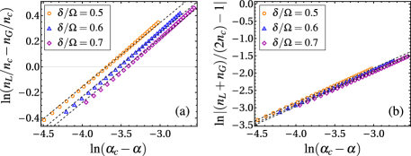
Fig. S3: Universal critical scaling for the relative (a) and averaged (b) densities of liquid and gas at their coexistence. Here we consider the liquid-gas coexistence tuned by $\alpha$. The slopes of all fitting lines in the (a) are $1/2$ and in (b) are $1$, giving the universal exponents $\lambda=1/2$ and $\xi=1$. $\beta,\eta$ are the same as in Fig.4.

References

• (1) P. M. Chaikin and T. C. Lubensky, Principles of Condensed Matter Physics (Cambridge University Press, Cambridge, 1995).
• (2) J. Richert, P. Wagner, Microscopic model approaches to fragmentation of nuclei and phase transitions in nuclear matter, Phys. Rep. 350, 1 (2001).
• (3) V. A. Karnaukhov, H. Oeschler, S. P. Avdeyev, E. V. Duginova, V. K. Rodionov, A. Budzanowski, W. Karcz, O. V. Bochkarev, E. A. Kuzmin, L. V. Chulkov, E. Norbeck, and A. S. Botvina, Critical temperature for the nuclear liquid-gas phase transition, Phys. Rev. C 67, 011601(R) (2003).
• (4) V. Vovchenko, M. I. Gorenstein, H. Stoecker, van der Waals Interactions in Hadron Resonance Gas: From Nuclear Matter to Lattice QCD, Phys. Rev. Lett. 118, 182301 (2017).
• (5) Michael E. Cates and Julien Tailleur, Motility-Induced Phase Separation, Annu. Rev. Condens. Matter Phys. 6, 219 (2015).
• (6) Ahmad K. Omar, Katherine Klymko, Trevor GrandPre, Phillip L. Geissler, Phase Diagram of Active Brownian Spheres: Crystallization and the Metastability of Motility-Induced Phase Separation, Phys. Rev. Lett. 126, 188002 (2021).
• (7) L. D. Landau and E. M. Lifshitz, Statistical Physics (Part 1), 3rd edition (Elsevier, Singapore, 2007).
• (8) K. Huang, Statistical Mechanics, 2nd edition (Wiley, New York, 1991).
• (9) M. D. Miller, L. H. Nosanow, L. J. Parish, Liquid-to-Gas Phase Transition in Quantum Systems at Zero Temperature, Phys. Rev. Lett. 35, 581 (1975).
• (10) M. D. Miller, L. H. Nosanow, Liquid-to-Gas Phase Transitions in Two-Dimensional Quantum Systems at Zero Temperature, Journal of Low Temperature Physics, 32, 145 (1978).
• (11) I. Ferrier-Barbut, H. Kadau, M. Schmitt, M. Wenzel, and T. Pfau, Observation of Quantum Droplets in a Strongly Dipolar Bose Gas, Phys. Rev. Lett. 116, 215301 (2016).
• (12) M. Schmitt, M. Wenzel, F. Böttcher, I. Ferrier-Barbut, and T. Pfau, Self-bound droplets of a dilute magnetic quantum liquid, Nature 539, 259 (2016).
• (13) L. Chomaz, S. Baier, D. Petter, M. J. Mark, F. Wächtler, L. Santos, and F. Ferlaino, Quantum-Fluctuation-Driven Crossover from a Dilute Bose-Einstein Condensate to a Macrodroplet in a Dipolar Quantum Fluid, Phys. Rev. X 6, 041039 (2016).
• (14) L. Tanzi, E. Lucioni, F. Fama, J. Catani, A. Fioretti, C. Gabbanini, R. N. Bisset, L. Santos, and G. Modugno, Observation of a Dipolar Quantum Gas with Metastable Supersolid Properties, Phys. Rev. Lett. 122, 130405 (2019).
• (15) F. Böttcher, J.-N. Schmidt, M. Wenzel, J. Hertkorn, M. Guo, T. Langen, and T. Pfau, Transient Supersolid Properties in an Array of Dipolar Quantum Droplets, Phys. Rev. X 9, 011051 (2019).
• (16) L. Chomaz, D. Petter, P. Ilzhöfer, G. Natale, A. Trautmann, C. Politi, G. Durastante, R.M.W. van Bijnen, A. Patscheider, M. Sohmen, M.J. Mark, and F. Ferlaino, Long-Lived and Transient Supersolid Behaviors in Dipolar Quantum Gases, Phys. Rev. X 9, 021012 (2019).
• (17) C. R. Cabrera, L. Tanzi, J. Sanz, B. Naylor, P. Thomas, P. Cheiney, and L. Tarruell, Quantum liquid droplets in a mixture of Bose-Einstein condensates, Science 359, 301 (2018).
• (18) P. Cheiney, C. R. Cabrera, J. Sanz, B. Naylor, L. Tanzi, and L. Tarruell, Bright Soliton to Quantum Droplet Transition in a Mixture of Bose-Einstein Condensates, Phys. Rev. Lett. 120, 135301 (2018).
• (19) G. Semeghini, G. Ferioli, L. Masi, C. Mazzinghi, L. Wolswijk, F. Minardi, M. Modugno, G. Modugno, M. Inguscio, and M. Fattori, Self-Bound Quantum Droplets of Atomic Mixtures in Free Space, Phys. Rev. Lett. 120, 235301 (2018).
• (20) C. D’Errico, A. Burchianti, M. Prevedelli, L. Salasnich, F. Ancilotto, M. Modugno, F. Minardi, and C. Fort, Observation of quantum droplets in a heteronuclear bosonic mixture, Phys. Rev. Res. 1, 033155 (2019).
• (21) Z. Guo, F. Jia, L. Li, Y. Ma, J. M. Hutson, X. Cui, and D. Wang, Lee-Huang-Yang effects in the ultracold mixture of 23Na and 87Rb with attractive interspecies interactions, Phys. Rev. Res. 3, 033247 (2021).
• (22) D. S. Petrov, Quantum Mechanical Stabilization of a Collapsing Bose-Bose Mixture, Phys. Rev. Lett. 115, 155302 (2015).
• (23) For thermodynamic boson mixtures, the equilibrium density of quantum droplet continuously goes to zero (gas) as the system is tuned across the mean-field collapse pointPetrov2015:QuantumMechanicalStabilization . This marks a continuous, rather than a first-order, liquid-gas transition at this point.
• (24) M. Ota and G. Astrakharchik, Beyond Lee-Huang-Yang description of self-bound Bose mixtures, SciPost Phys. 9, 020 (2020).
• (25) J. Wang, X.-J. Liu, and H. Hu, Ultradilute Self-Bound Quantum Droplets in Bose–Bose Mixtures at Finite Temperature, Chinese Phys. B 30, 010306 (2021).
• (26) N. Guebli and A. Boudjemâa, Quantum self-bound droplets in Bose-Bose mixtures: Effects of higher-order quantum and thermal fluctuations, Phys. Rev. A 104, 023310 (2021).
• (27) E. Nicklas, H. Strobel, T. Zibold, C. Gross, B. A. Malomed, P. G. Kevrekidis, and M. K. Oberthaler, Rabi Flopping Induces Spatial Demixing Dynamics, Phys. Rev. Lett. 107, 193001 (2011).
• (28) L. Lavoine, A. Hammond, A. Recati, D. S. Petrov, and T. Bourdel, Beyond-Mean-Field Effects in Rabi-Coupled Two-Component Bose-Einstein Condensate, Phys. Rev. Lett. 127, 203402 (2021).
• (29) A. Hammond, L. Lavoine, and T. Bourdel, Tunable Three-Body Interactions in Driven Two-Component Bose-Einstein Condensates, Phys. Rev. Lett. 128, 083401 (2022).
• (30) J. Sanz, A. Frölian, C. S. Chisholm, C. R. Cabrera, and L. Tarruell, Interaction Control and Bright Solitons in Coherently Coupled Bose-Einstein Condensates, Phys. Rev. Lett. 128, 013201 (2022).
• (31) R. Cominotti, A. Berti, C. Dulin, C. Rogora, G. Lamporesi, L. Carusotto, A. Recati, A. Zenesini, G. Ferrari, Revealing the ferromagnetic phase transition in an extended two-component atomic superfluid, arxiv:2209.13235.
• (32) See supplementary materials for more details.
• (33) T. Mithun, A. Maluckov, K. Kasamatsu, B. A. Malomed, and A. Khare, Modulational instability, intercomponent asymmetry, and formation of quantum droplets in one-dimensional binary Bose gases, Symmetry 12, 174 (2020).
• (34) M. N. Tengstrand and S. M. Reimann, Droplet-superfluid compounds in binary bosonic mixtures, Phys. Rev. A 105, 033319 (2022).
• (35) T. A. Flynn, L. Parisi, T. P. Billam, and N. G. Parker, Quantum Droplets in Imbalanced Atomic Mixtures, arxiv: 2209.04318.
• (36) L. He, H. Li, W. Yi, Z.-Q. Yu, Quantum criticality of liquid-gas transition in a binary boson mixture, arxiv:2209.13559.

References

• (1) Q. Gu and L. Yin, Phonon stability and sound velocity of quantum droplets in a boson mixture, Phys. Rev. B 102, 220503(R) (2020).
• (2) L. Lavoine, A. Hammond, A. Recati, D. S. Petrov, and T. Bourdel, Beyond-Mean-Field Effects in Rabi-Coupled Two-Component Bose-Einstein Condensate, Phys. Rev. Lett. 127, 203402 (2021).
• (3) P. M. Chaikin and T. C. Lubensky, Principles of Condensed Matter Physics (Cambridge University Press, Cambridge, 1995).