Metadata Archaeology: Unearthing Data Subsets
by Leveraging Training Dynamics

Abstract

Modern machine learning research relies on relatively few carefully curated datasets. Even in these datasets, and typically in ‘untidy’ or raw data, practitioners are faced with significant issues of data quality and diversity which can be prohibitively labor intensive to address. Existing methods for dealing with these challenges tend to make strong assumptions about the particular issues at play, and often require a priori knowledge or metadata such as domain labels. Our work is orthogonal to these methods: we instead focus on providing a unified and efficient framework for Metadata Archaeology – uncovering and inferring metadata of examples in a dataset. We curate different subsets of data that might exist in a dataset (e.g. mislabeled, atypical, or out-of-distribution examples) using simple transformations, and leverage differences in learning dynamics between these probe suites to infer metadata of interest. Our method is on par with far more sophisticated mitigation methods across different tasks: identifying and correcting mislabeled examples, classifying minority-group samples, prioritizing points relevant for training and enabling scalable human auditing of relevant examples.

1 Introduction

Modern machine learning is characterized by ever-larger datasets and models. The expanding scale has produced impressive progress [67, 30, 52] yet presents both optimization and auditing challenges. Real-world dataset collection techniques often result in significant label noise [64], and can present significant numbers of redundant, corrupted, or duplicate inputs [12]. Scaling the size of our datasets makes detailed human analysis and auditing labor-intensive, and often simply infeasible. These realities motivate a consideration of how to efficiently characterize different aspects of the data distribution.

Prior work has developed a rough taxonomy of data properties, or metadata which different examples might exhibit, including but not limited to: noisy [68, 71, 62, 63], atypical [25, 10, 21, 60], challenging [24, 3, 8, 49, 2], prototypical or core subset selection [49, 55, 56, 27] and out-of-distribution [36]. While important progress has been made on some of these metadata categories individually, these categories are typically addressed in isolation reflecting an overly strong assumption that only one, known issue is at play in a given dataset.

For example, considerable work has focused on the issue of label noise. A simple yet widely-used approach to mitigate label noise is to remove the impacted data examples [50]. However, it has been shown that it is challenging to distinguish difficult examples from noisy ones, which often leads to useful data being thrown away when both noisy and atypical examples are present [66, 61].

Figure 1: Examples surfaced through the use of MAP-D on ImageNet train set. Column title is the ground truth class, row title is the metadata category assigned by MAP-D. MAP-D performs metadata archaeology by curating a probe set and then probing for similar examples based on training dynamics. This approach can bring to light biases, mislabelled examples, and other dataset issues.

Meanwhile, loss-based prioritization [28, 31] techniques essentially do the opposite – these techniques upweight high loss examples, assuming these examples are challenging yet learnable. These methods have been shown to quickly degrade in performance in the presence of even small amounts of noise since upweighting noisy samples hurts generalization [26, 49].

The underlying issue with such approaches is the assumption of a single, known type of data issue. Interventions are often structured to identify examples as simple vs. challenging, clean vs. noisy, typical vs. atypical, in-distribution vs. out-of-distribution etc. However, large scale datasets may present subsets with many different properties. In these settings, understanding the interactions between an intervention and many different subsets of interest can help prevent points of failure. Moreover, relaxing the notion that all these properties are treated independently allows us to capture realistic scenarios where multiple metadata annotations can apply to the same datapoint. For example, a challenging example may be so because it is atypical.

In this work, we are interested in moving away from a siloed treatment of different data properties. We use the term Metadata Archaeology to describe the problem of inferring metadata across a more complete data taxonomy. Our approach, which we term Metadata Archaeology via Probe Dynamics (MAP-D), leverages distinct differences in training dynamics for different curated subsets to enable specialized treatment and effective labelling of different metadata categories. Our methods of constructing these probes are general enough that the same probe category can be crafted efficiently for many different datasets with limited domain-specific knowledge.

We present consistent results across six image classification datasets, CIFAR-10/CIFAR-100 [35], ImageNet [14], Waterbirds [54], CelebA [40] , Clothing1M [69] and two models from the ResNet family [22]. Our simple approach is competitive with far more complex mitigation techniques designed to only treat one type of metadata in isolation. Furthermore, it outperforms other methods in settings dealing with multiple sources of uncertainty simultaneously. We summarize our contributions as:

• We propose Metadata Archeology, a unifying and general framework for uncovering latent metadata categories.

• We introduce and validate the approach of Metadata Archaeology via Probe Dynamics (MAP-D): leveraging the training dynamics of curated data subsets called probe suites to infer other examples’ metadata.

• We show how MAP-D could be leveraged to audit large-scale datasets or debug model training, with negligible added cost - see Figure 1. This is in contrast to prior work which presents a siloed treatment of different data properties.

• We use MAP-D to identify and correct mislabeled examples in a dataset. Despite its simplicity, MAP-D is on-par with far more sophisticated methods, while enabling natural extension to an arbitrary number of modes.

• Finally, we show how to use MAP-D to identify minority group samples, or surface examples for data-efficient prioritized training.

2 Metadata Archaeology via Probe Dynamics (MAP-D)

Metadata is data about data, for instance specifying when, where, or how an example was collected. This could include the provenance of the data, or information about its quality (e.g. indicating that it has been corrupted by some form of noise). An important distinguishing characteristic of metadata is that it can be relational, explaining how an example compares to others. For instance, whether an example is typical or atypical, belongs to a minority class, or is out-of-distribution (OOD), are all dependent on the entire data distribution.

The problem of metadata archaeology is the inference of metadata $m\subset\mathcal{M}$ given a dataset $\mathcal{D}$. While methods for inferring $m$ might also be useful for semi-supervised labelling or more traditional feature engineering, and vice versa, it is the relational nature of metadata that makes this problem unique and often computationally expensive.

2.1 Methodology

Metadata Archaeology via Probe Dynamics (MAP-D), leverages differences in the statistics of learning curves across metadata features to infer the metadata of previously unseen examples.

We consider a model which learns a function $f_{\theta}:\mathcal{X}\mapsto\mathcal{Y}$ with trainable weights $\theta$. Given the training dataset $\mathcal{D}$, $f_{\theta}$ optimizes a set of weights $\theta^{*}$ by minimizing an objective function $L$ with loss $l$ for each example.

We assume that the learner has access to two types of samples for training. First is a training set $\mathcal{D}$:

$$\mathcal{D}:=\big{\{}(x_{1},y_{1}),\dots,(x_{N},y_{N})\big{\}}\subset\mathcal{X}\times\mathcal{Y}$$ (1)

where $\mathcal{X}$ represents the data space and $\mathcal{Y}$ the set of outcomes associated with the respective instances. Examples in the data space are also assumed to have associated, but unobserved, metadata $m\subset\mathcal{M}$.

Secondly, we assume the learner to also have access to a small curated subset of $j$ samples ($j\leq N$; typically $j\ll N$) associated with metadata $m\subset\mathcal{M}$, i.e.:

$$\mathcal{D}_{m}:=\{(x_{1},y_{1},m_{1}),\dots,(x_{j},y_{j},m_{j})\}\subset\mathcal{X}\times\mathcal{Y}\times\mathcal{M}\enspace$$ (2)

We refer to these curated subsets as probe suites. A key criteria is for our method to require very few annotated probe examples ($j\ll N$). In this work, we focus on probe suits which can be constructed algorithmically, as human annotations of metadata require costly human effort to maintain.

2.1.1 Assigning Metadata Features to Unseen Examples

MAP-D works by comparing the performance of a given example to the learning curves typical of a given probe type. Our approach is motivated by the observation that different types of examples often exhibit very different learning dynamics over the course of training (see Figure 3). In an empirical risk minimization setting, we minimize the average training loss across all training points.

$$L_{(}\theta)=\frac{1}{N}\sum_{i=1}^{N}\ell\left(x_{i},y_{i};\theta\right)$$

However, performance on a given subset will differ from the average error. Specifically, we firstly evaluate the learning curves of individual examples:

$$\textbf{s}_{i}^{t}:=\left(\ell(x_{i},y_{i};\theta_{1}),\ell(x_{i},y_{i};\theta_{2}),...,\ell(x_{i},y_{i};\theta_{t})\mid(x_{i},y_{i})\in\mathcal{D}\right)$$ (3)

where $\textbf{s}_{i}^{t}$ denotes the learning curve for the i^th training example, and $t$ is the current epoch. We then track the per-example performance on probes g for each metadata category $m\in\{m_{1},\dots,m_{|\mathcal{M}|}\}$, and refer to each probe as g($m$).

$$\textbf{g}_{j}^{t}(m):=\left(\ell(x_{j},y_{j};\theta_{1}),\ell(x_{j},y_{j};\theta_{2}),...,\ell(x_{j},y_{j};\theta_{t})\mid(x_{j},y_{j})\in\mathcal{D}_{m}\right)$$ (4)

where $\textbf{g}_{j}^{t}(m)$ denotes the learning curve computed on the j^th example chosen from a given probe category $m$. We use $\mathcal{D}_{g}$ as shorthand to refer to the set of all these trajectories for the different probe categories along with the category identity.

$$\mathcal{D}_{\textbf{g}}:=\left((\textbf{g}_{1}^{t}(m_{1}),m_{1}),\dots,(\textbf{g}_{|m_{1}|}^{t}(m_{1}),m_{1}),(\textbf{g}_{1}^{t}(m_{2}),m_{2}),\dots,(\textbf{g}_{|m_{|\mathcal{M}|}|}^{t}(m_{|\mathcal{M}|}),m_{|\mathcal{M}|})\right)$$ (5)

where $|m_{c}|$ refers the number of examples belonging to the metadata category $m_{c}$.

We assign metadata features to an unseen data point by looking up the example’s nearest neighbour from $\mathcal{D}_{\textbf{g}}$, using the Euclidean distance. In general, assignment of probe type could be done via any classification algorithm. However, in this work we use $k$-NN ($k$-Nearest Neighbours) for its simplicity, interpretability and the ability to compute the probability of multiple different metadata features.

$$p(m\mid\textbf{s}_{i}^{t})=\frac{1}{k}\;\sum_{(\mathbf{g},\hat{m})\;\in\;\textsc{NN}(\textbf{s}_{i}^{t},\mathcal{D}_{\textbf{g}},k)}\mathbbm{1}_{\hat{m}=m}$$ (6)

where $p(m\mid\textbf{s}_{i}^{t})$ is the probability assigned to probe category $m$ based on the $k$ nearest neighbors for learning curve of the i^th training example from the dataset, and $\textsc{NN}(\textbf{s}_{i}^{t},\mathcal{D}_{g},k)$ represents the top-$k$ nearest neighbors for $\textbf{s}_{i}^{t}$ from $\mathcal{D}_{\textbf{g}}$ (probe trajectory dataset) based on Euclidean distance between the loss trajectories for all the probe examples and the given training example. We fix $k$=20 in all our experiments.

This distribution over probes (i.e metadata features) may be of primary interest, but we are sometimes also interested in seeing which metadata feature a given example most strongly corresponds to; in this case, we compute the argmax:

$$m^{\prime}_{i}=\operatorname*{arg\,max}_{m\in\mathcal{M}}\;p(m\mid\textbf{s}_{i}^{t})$$ (7)

where $m^{\prime}_{i}$ denotes the assignment of the i^th example to a particular probe category.

We include the probe examples in the training set unless specified otherwise; excluding them in training can result in a drift in trajectories, and including them allows tracking of training dynamics.

Black bear

(a) Typical

Dishwasher

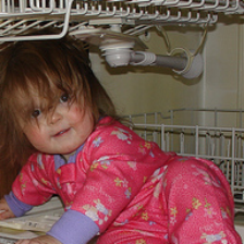
(b) Atypical

School bus

(c) Corrupted

Mud turtle

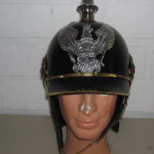
(d) Rand Label

Jeep

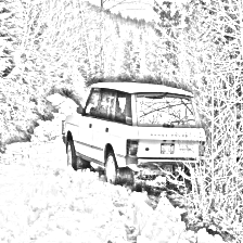
(e) OOD

Loafer

(f) Rand Input

Figure 2: An illustration of samples from our curated probes. Creating our probe suites requires no human annotation. We curate different subsets of data that might exist in a dataset including (a) typical, (b) atypical, (c) corrupted, (d) mislabeled, (e) out-of-distribution, and (f) random input examples, using simple transformations or existing scoring mechanisms.

2.2 Probe Suite Curation

While probe suites can be constructed using human annotations, this can be very expensive to annotate [4, 65]. In many situations where auditing is desirable (e.g. toxic or unsafe content screening), extensive human labour is undesirable or even unethical [58, 57]. Hence, in this work, we focus on probes that can be computationally constructed for arbitrary datasets – largely by using simple transformations and little domain-specific knowledge. We emphasize that our probe suite is not meant to be exhaustive, but to provide enough variety in metadata features to demonstrate the merits of metadata archaeology.

We visualize these probes in Figure 2, and describe below:

1. Typical We quantify typicality by thresholding samples with the top consistency scores from Jiang et al. [29] across all datasets. The consistency score is a measure of expected classification performance on a held-out instance given training sets of varying size sampled from the training distribution.

2. Atypical Similarly, atypicality is quantified as samples with the lowest consistency scores from Jiang et al. [29].

3. Random Labels Examples in this probe have their labels replaced with uniform random labels, modelling label noise.

4. Random Inputs & Labels These noisy probes are comprised of uniform $\mathcal{U}(0,1)$ noise sampled independently for every dimension of the input. We also randomly assign labels to these samples.

5. Corrupted Inputs Corrupted examples are constructed by adding Gaussian noise with 0 mean and 0.1 standard deviation for CIFAR-10/100 and 0.25 standard deviation for ImageNet. These values were chosen to make the inputs as noisy as possible while still being (mostly) recognizable to humans.

We curate 250 training examples for each probe category. For categories other than Typical/Atypical, we sample examples at random and then apply the corresponding transformations. All of the probes are then included during training so that we can study their training dynamics. We also curate 250 test examples for each probe category to evaluate the accuracy of our nearest neighbor assignment of metadata to unseen data points, where we know the true underlying metadata.

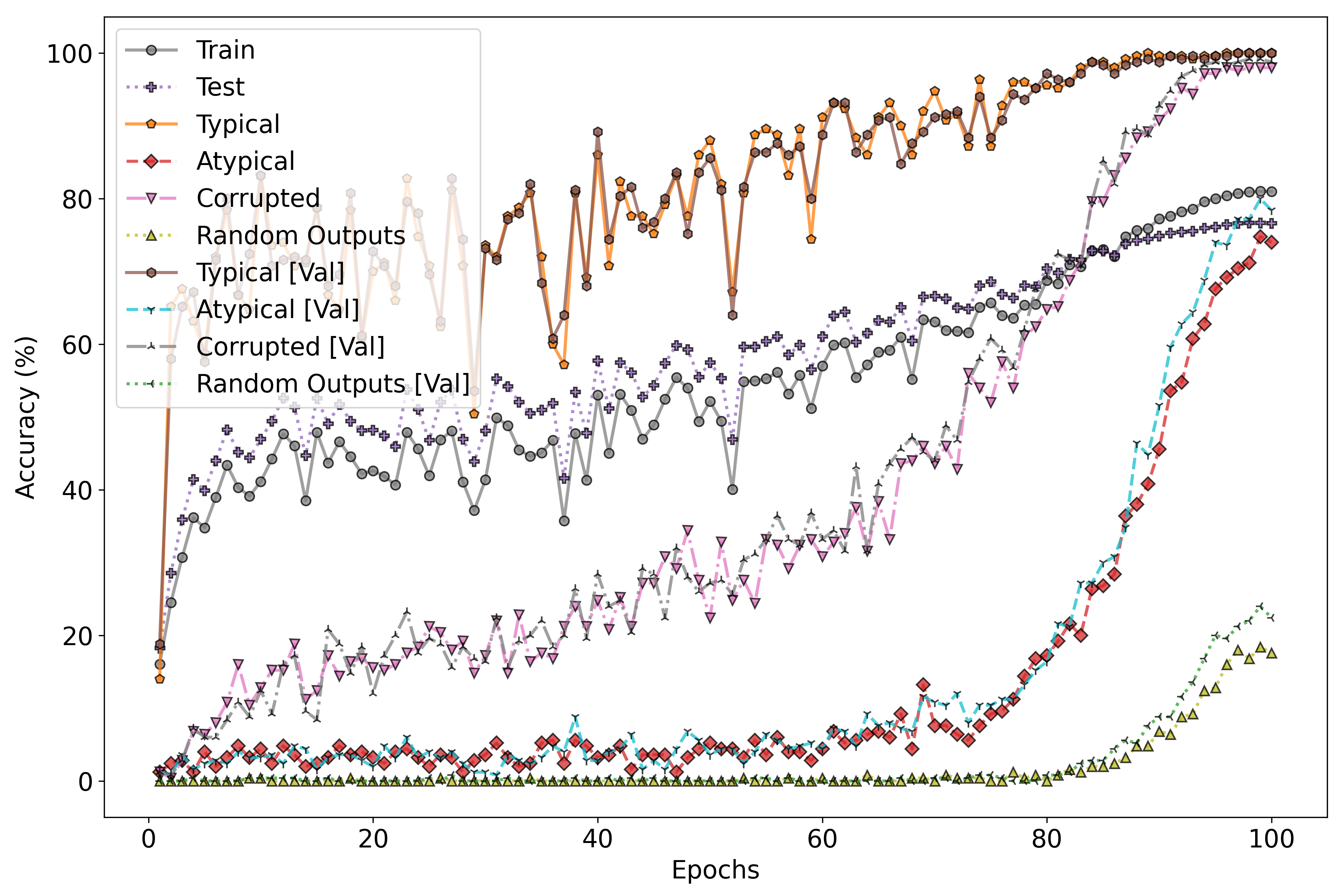
(a)

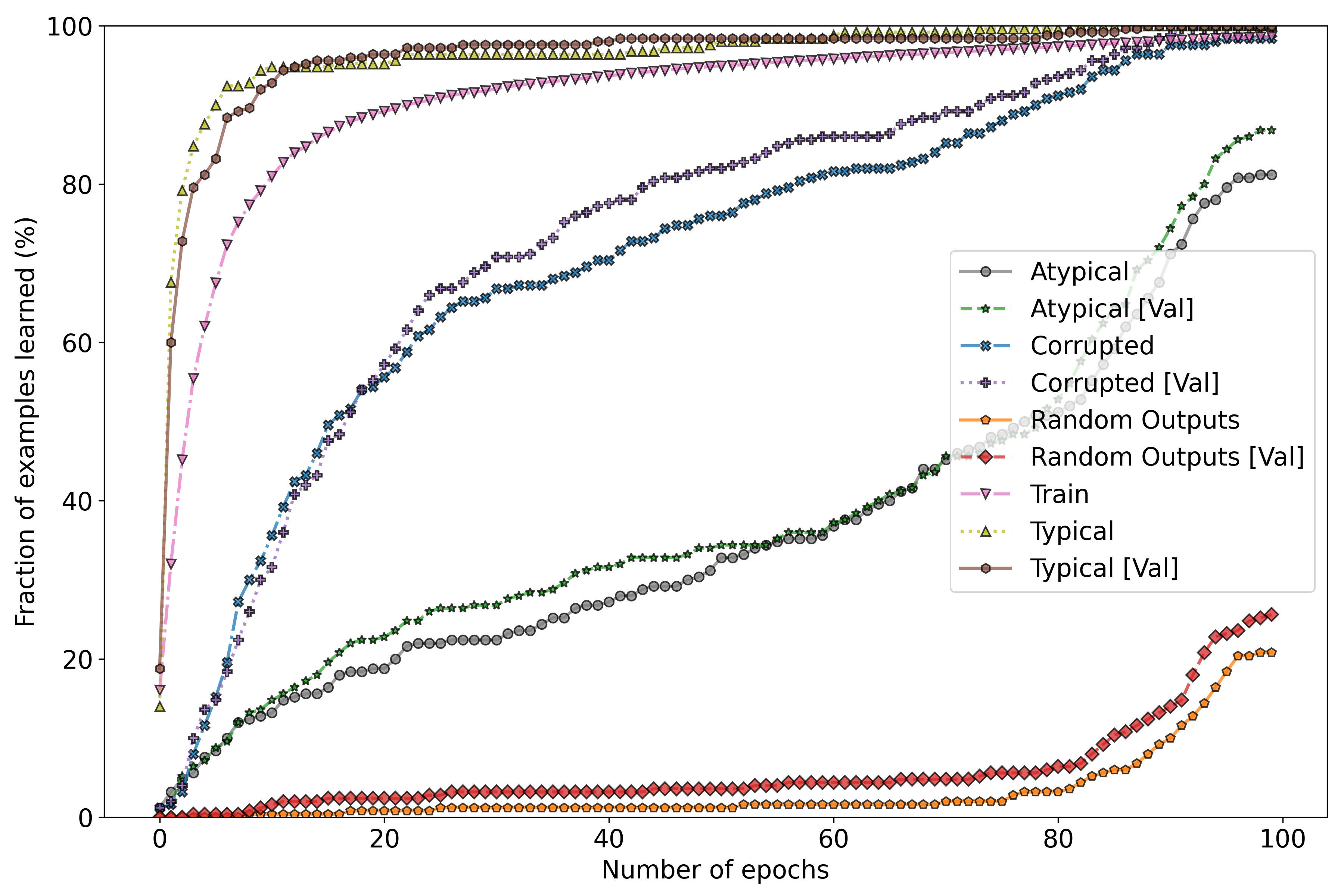
(b)

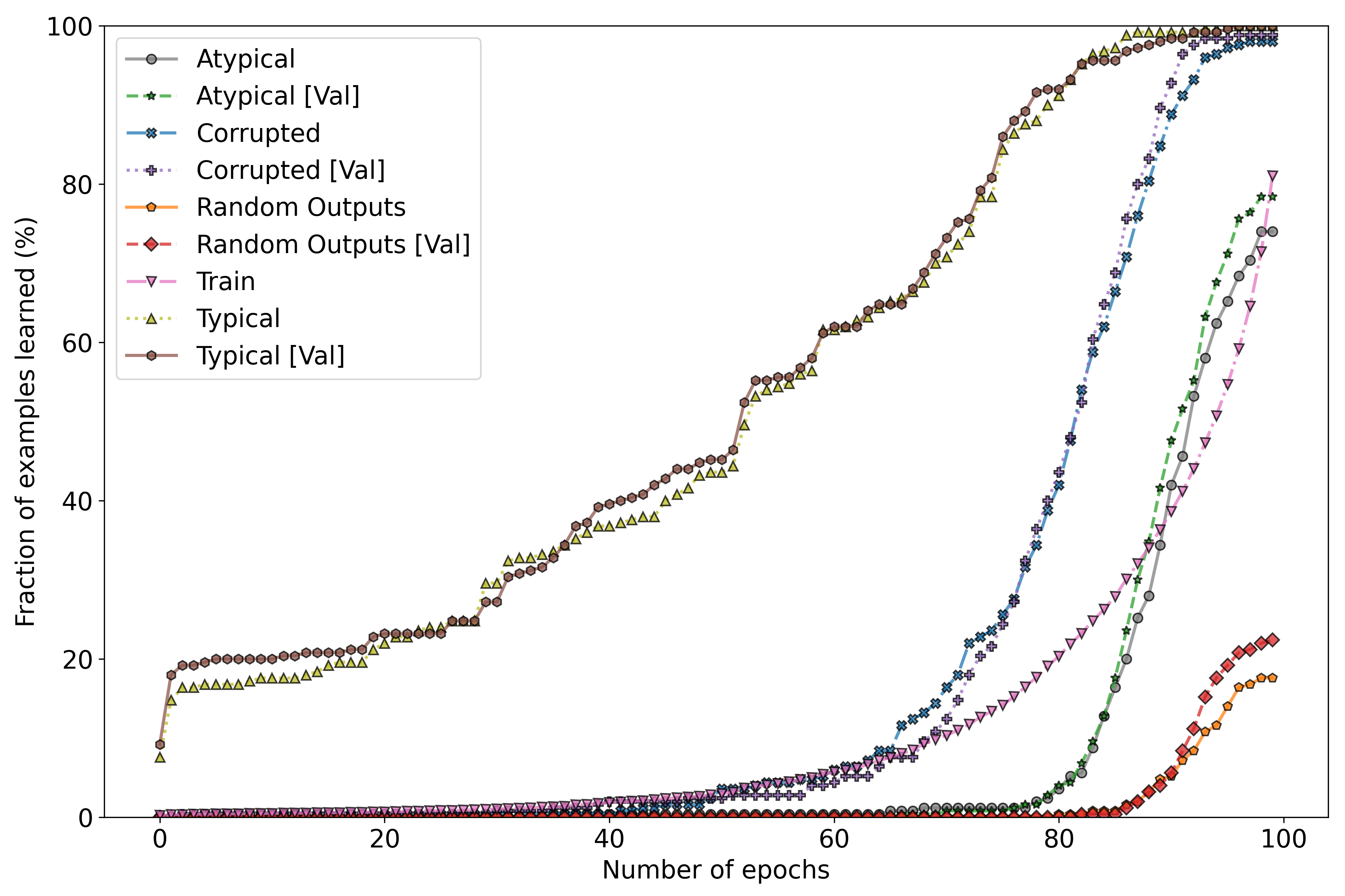
(c)

(d)

(e)

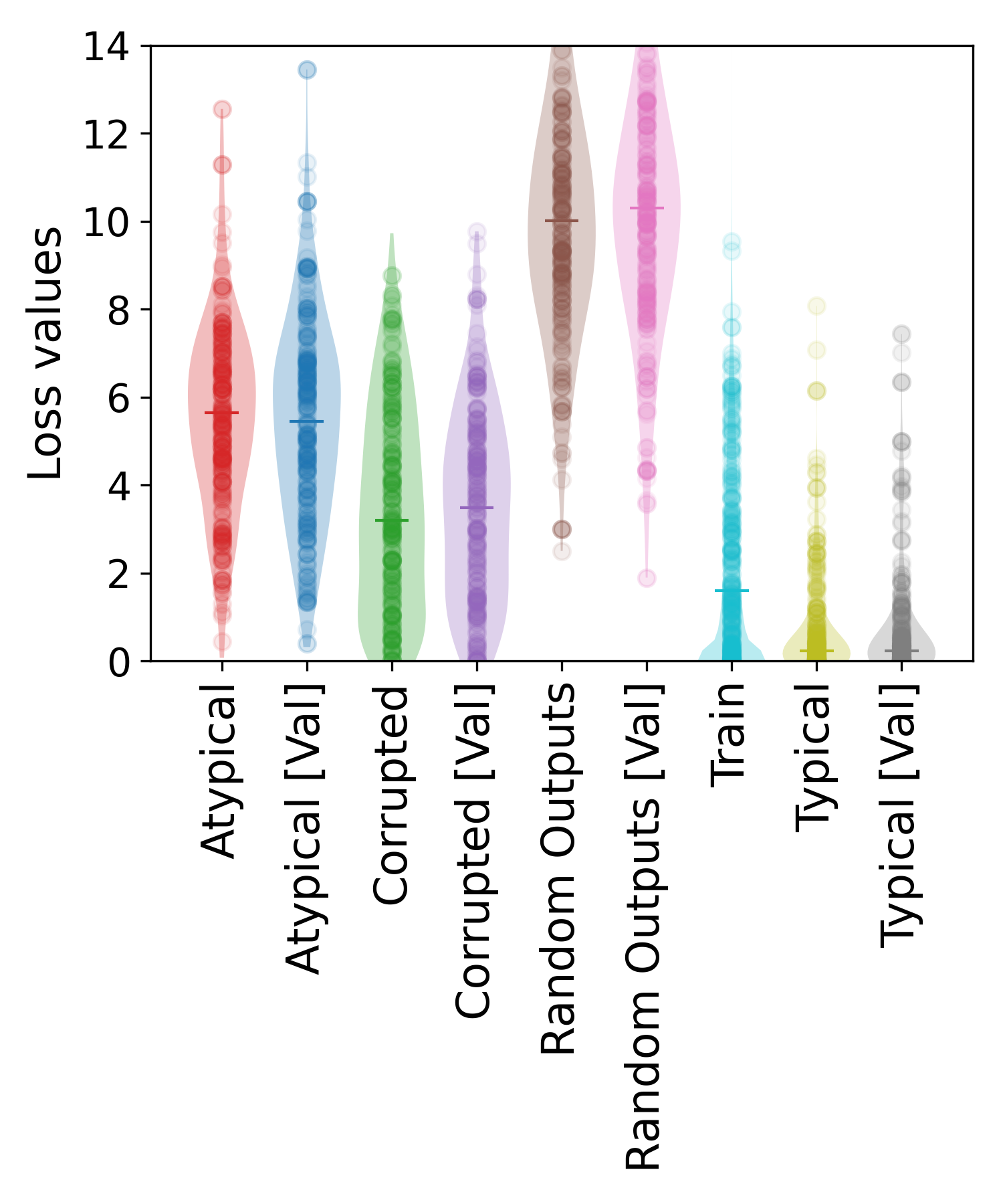
(f)

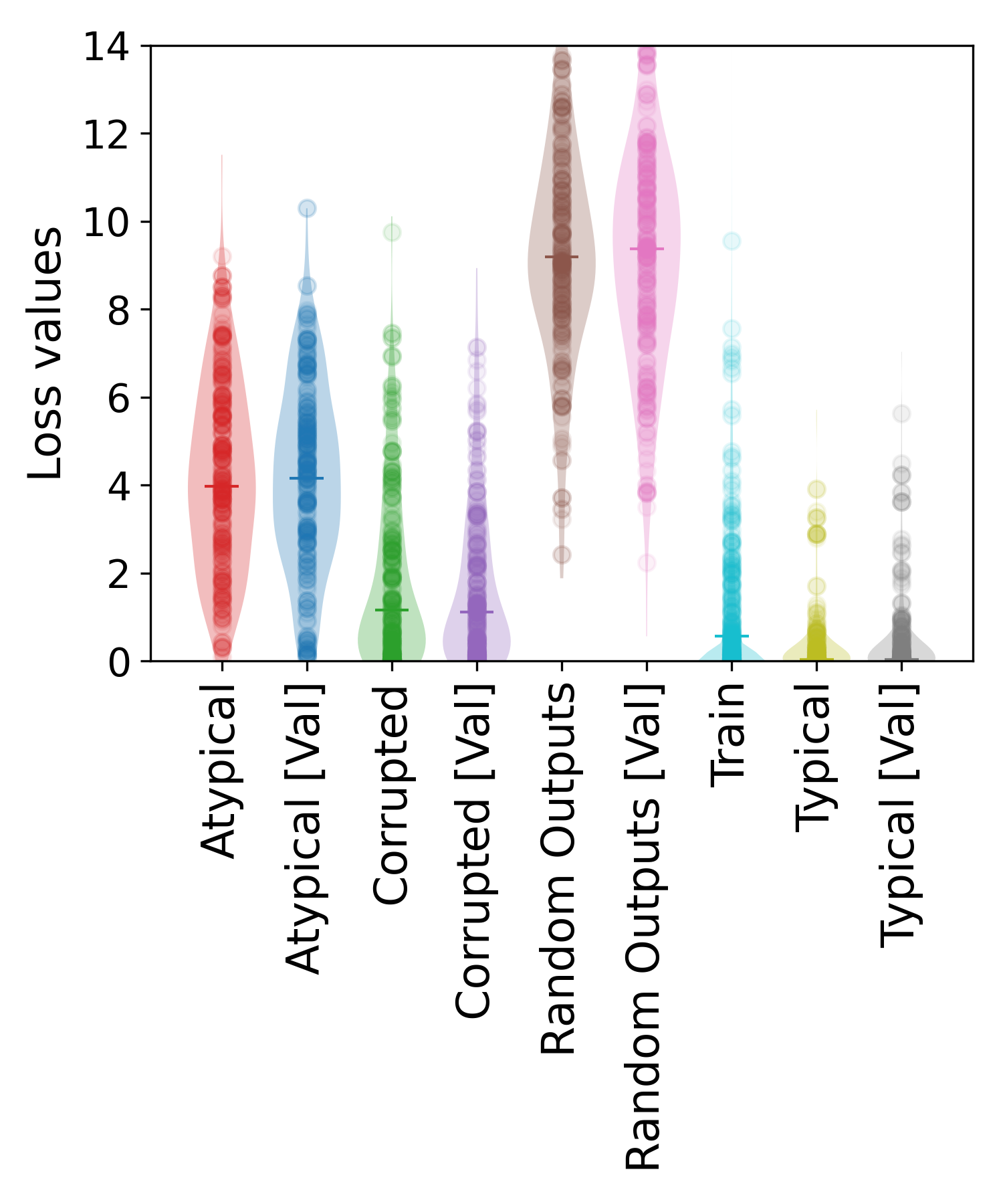
(g)

(h)

Figure 3: Probe categories are distinguishable via learning dynamics of a ResNet-50 trained on ImageNet, validating the approach of MAP-D. For each of the probe categories and at each epoch, we plot (a) each probe’s average accuracy; (b) the cumulative fraction of examples once predicted correctly by the nth epoch; and (c) the fraction that remain predicted correctly on all subsequent epochs. Bottom plots (d)-(h) show the spread of losses at various epochs of training.

3 Experiments and Discussion

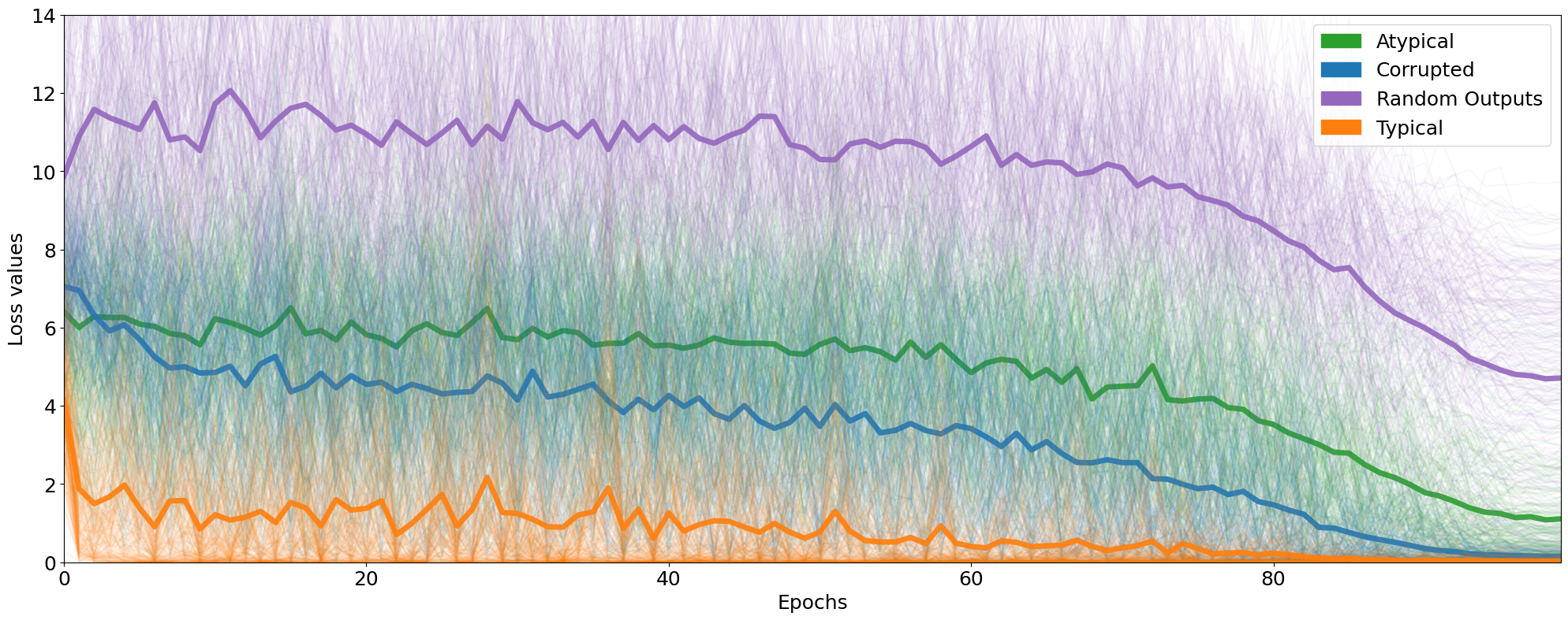
(a)

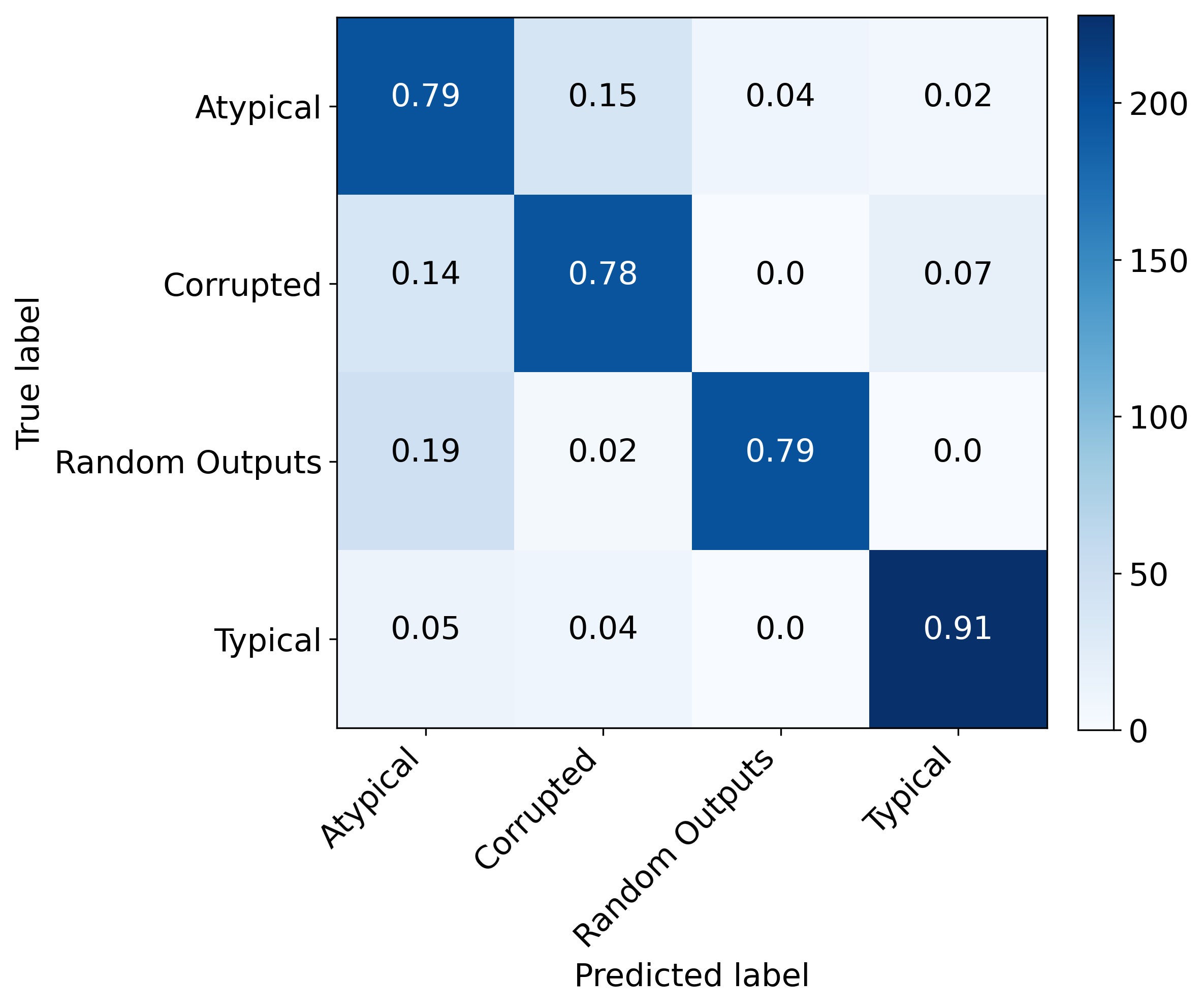
(b)

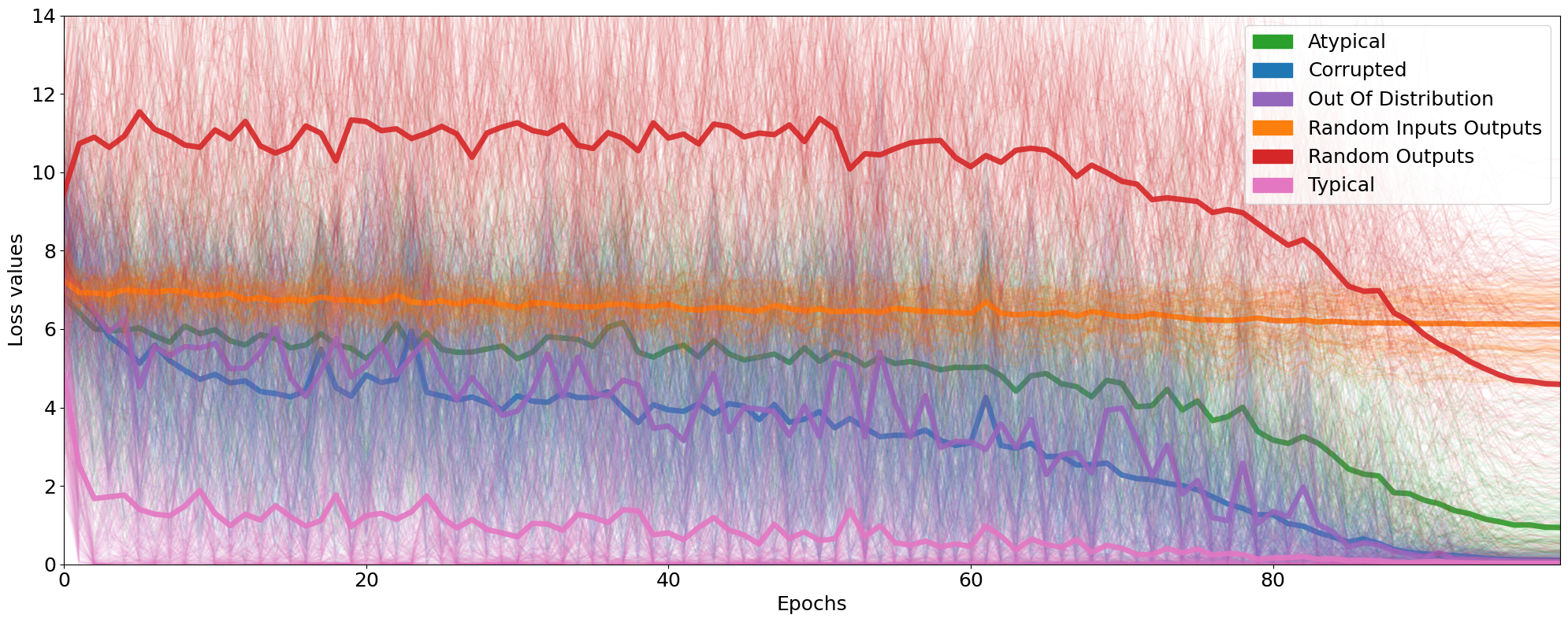
(c)

(d)

Figure 4: Sanity check showing performance of MAP-D on the probe suite test set using ResNet-50 on ImageNet, where we know the ground-truth metadata. (a) and (c) Solid line shows the mean learning curve while translucent lines are randomly sampled 250 individual trajectories for each probe category. Again, the separation of different probes is evident both in the dynamics over the course of training. (b) and (d) show confusion matrices between the true vs. predicted metadata features, demonstrating strong performance of the probes.

In the following sections, we perform experiments across 6 datasets: CIFAR-10/100, ImageNet, Waterbirds, CelebA, and Clothing1M. For details regarding the experimental setup, see Appendix A. We first evaluate convergence dynamics of different probe suites (Section 3.1), validating the approach of MAP-D. We then qualitatively demonstrate the ability to audit datasets using MAP-D (Section 3.2), and evaluate performance on a variety of downstream tasks: noise correction (Section 3.3), prioritizing points for training (Section 3.4), and identifying minority-group samples (Section 3.5).

3.1 Probe Suite Convergence Dynamics

In Figure 3, we present the training dynamics on the probe suites given a ResNet-50 model on ImageNet. For all datasets, we observe that probe suites have distinct learning convergence trajectories, demonstrating the efficacy of leveraging differences in training dynamics for the identification of probe categories. We plot average 1) Probe Accuracy over the course of training, 2) the Percent First-Learned i.e. the percentage of samples which have been correctly classified once (even if that sample was be later forgotten) over the course of training, and 3) the Percent Consistently-Learned i.e. the percentage of samples which have been learned and will not be forgotten for the rest of training.

We observe consistent results across all dimensions. Across datasets, the Typical probe has the fastest rate of learning, whereas the Random Outputs probe has the slowest. When looking at Percent First-Learned in Figure 3, we see a very clear natural sorting by the difficulty of different probes, where natural examples are learned earlier as compared to corrupted examples with synthetic noise. Examples with random outputs are the hardest for the model.

We also observe that probe ranking in terms of both Percent First-Learned and Percent Consistently-Learned is stable across training, indicating that model dynamics can be leveraged consistently as a stable signal to distinguish between different subsets of the distribution at any point in training. These results motivate our use of learning curves as signal to infer unseen metadata.

3.2 Auditing Datasets

Typical

Balloon

Typical

Mountain Bike

Typical

Ambulance

Typical

Banana

Typical

Microwave

Typical

Toaster

Typical

iPod

Typical

Milk Can

Figure 5: Examples surfaced through the use of MAP-D on ImageNet train set using the Typical probe (first image in each set, highlighted with black border) and Random Output probe (next two images). Sub-caption indicates the ground truth class. This showcases the utility of MAP-D for exploring a dataset, showing what the model considers typical for a class as well as uncovering potentially problematic examples.

A key motivation of our work is that the large size of modern datasets means only a small fraction of datapoints can be economically inspected by humans. In safety-critical or otherwise sensitive domains such as health care diagnostics [70, 19, 7, 46], self-driving cars [44], hiring [13, 20], and many others, providing tools for domain experts to audit models is of great importance to ensure scalable oversight.

We apply MAP-D to infer the metadata features of the underlying dataset. In Fig. 1, we visualize class specific examples surfaced by MAP-D on the ImageNet train set. Our visualization shows that MAP-D helps to disambiguate effectively between different types of examples and can be used to narrow down the set of datapoints to prioritize for inspection. We observe clear semantic differences between the sets. In Fig. 1, we observe that examples surfaced as Typical are mostly well-centered images with a typical color scheme, where the only object in the image is the object of interest. Examples surfaced as Atypical present the object in unusual settings or vantage points, or feature differences in color scheme from the typical variants. We observe examples that would be hard for a human to classify using the Random Output probe category. For example, we see incorrectly labeled images of a digital watch, images where the labeled object is hardly visible, artistic and ambiguous images, and multi-object examples where several different labels may be appropriate. We visualize more examples from the Random Output probe category in Fig. 5.

As a sanity check, in Fig. 4 we also evaluate the performance of MAP-D on the held-out probe test set, where we know the true underlying metadata used to curate that example. In (a), we compute performance on the four probes which are most easily separable via learning curves, and find that model was able to achieve high detection performance ($\sim 81.9\%$ accuracy). When including OOD and Random Output probe categories (bottom row (c) and (d)), we observe from the learning curves that there is overlap in probe dynamics; these two categories are difficult to disambiguate, and as a result, we see a slight drop in overall performance ($\sim 78\%$).

3.3 Label Noise Correction

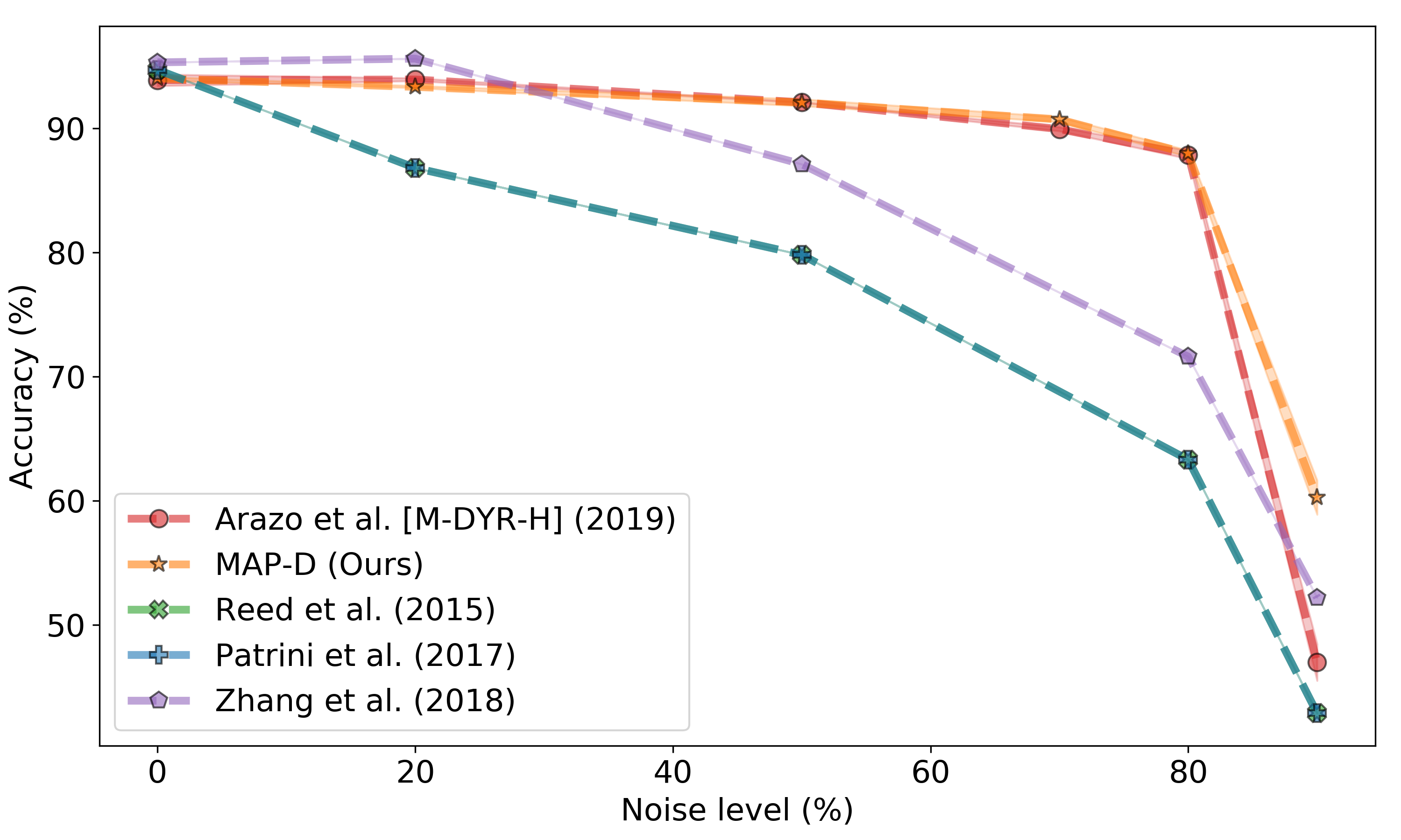
(a)

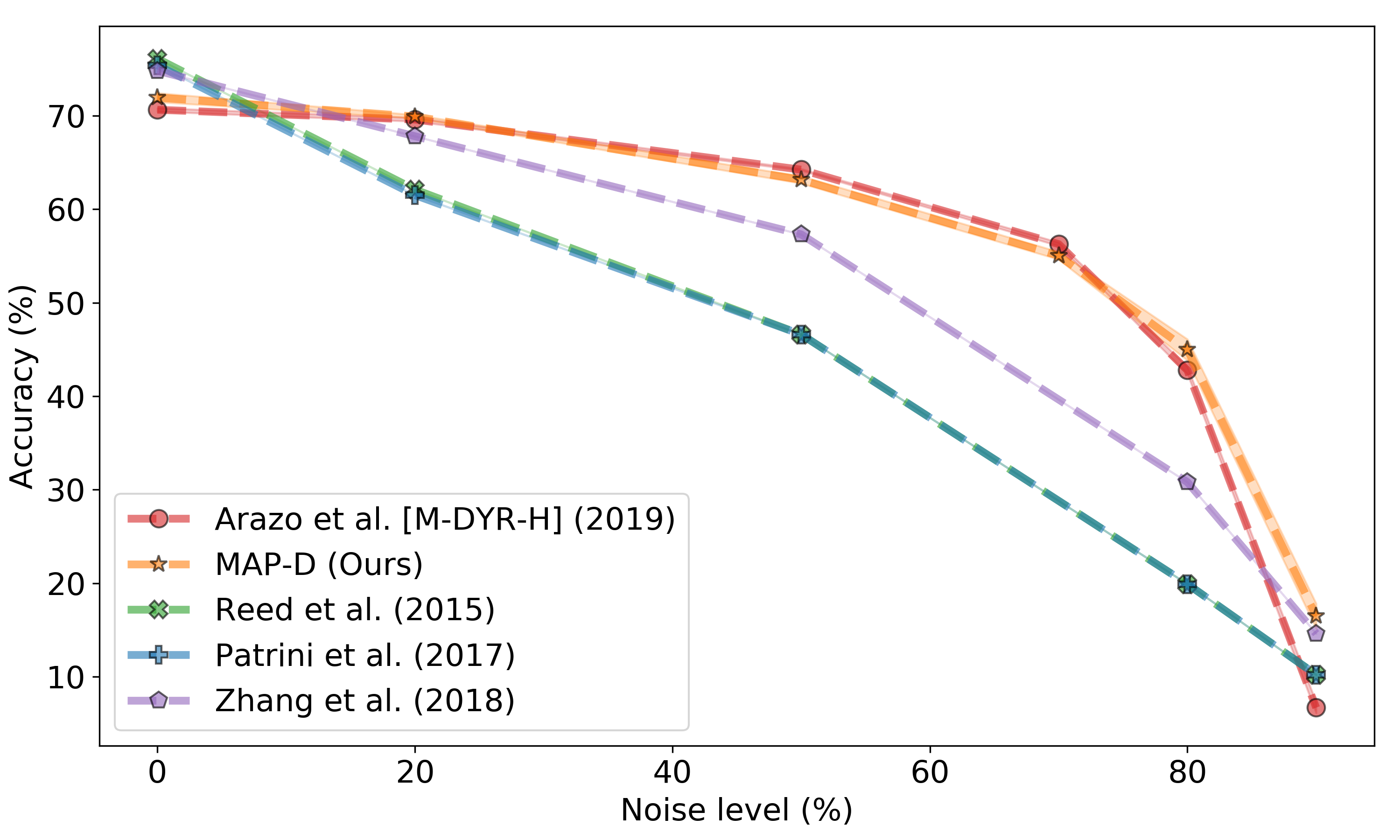
(b)

Figure 6: Comparison of different noise correction methods under the presence of label noise. Mean and standard deviation reported over 3 random runs. MAP-D is competitive with most other methods, many of which are particularly targeted towards this problem.

Here we apply MAP-D to detect and correct label noise, a data quality issue that has been heavily studied in prior works [73, 5, 6]. We benchmark against a series of different baselines (Arazo et al. [5], Zhang et al. [73], Patrini et al. [48], Reed et al. [51]), some of which are specifically developed to deal with label noise. We emphasize that our aim is not to develop a specialized technique for dealing with label noise, but to showcase that MAP-D, a general solution for metadata archaeology, also performs well on specialized tasks such as label correction.

To distinguish between clean and noisy samples using MAP-D, we add an additional random sample probe curated via a random sample from the (unmodified) underlying data, as a proxy for clean data. For this comparison, we follow the same experimental protocol as in [5] where all the methods we benchmark against are evaluated.

Concretely, for any label correction scheme, the actual label used for training is a convex combination of the original label and the model’s prediction based on the probability of the sample being either clean or noisy. Considering one-hot vectors, the correct label can be represented as:

$$\bar{y_{i}}=p(\texttt{clean}\mid\textbf{s}_{i}^{t})\times y_{i}+p(\texttt{noisy}\mid\textbf{s}_{i}^{t})\times\hat{y}_{i}$$ (8)

where $\bar{y_{i}}$ represents the corrected label used to train the model, $y_{i}$ represents the label present in the dataset weighted by the probability of the sample being clean $p(\texttt{clean}\mid\textbf{s}_{i}^{t})$, and $\hat{y}_{i}$ represents the model’s prediction (a one-hot vector computed via argmax rather than predicted probabilities) weighted by the probability of the sample being noisy $p(\texttt{noisy}\mid\textbf{s}_{i}^{t})$. Since we are only considering two classes, $p(\texttt{clean}\mid\textbf{s}_{i}^{t})=1-p(\texttt{noisy}\mid\textbf{s}_{i}^{t})$. We employ the online MAP-D trajectory scheme in this case, where the learning curve is computed given all prior epochs completed as of that point.

Despite the relative simplicity and generality of MAP-D, it generally performs as well as highly-engineereed methods developed specifically for this task. Our results are presented in Fig. 6. Specifically, at extremely high levels of noise, MAP-D performs significantly better on both CIFAR-10 and CIFAR-100 as compared to Arazo et al. [5] (CIFAR-10: $\sim 47\%$ vs $\sim 59\%$; CIFAR-100: $\sim 6.5\%$ vs $\sim 16.5\%$).

Number of epochs before noise correction

In the original setting proposed by  [5], the method requires pretraining for 105 epochs prior to label correction. We observe that a relative strength of MAP-D is the ability to forgo such prolonged pretraining while retraining for robust noisy example detection. We perform a simple experiment with a reduced number of pretraining epochs (10 instead of 105), with results presented in Fig. 7, demonstrating that there is only negligible impact of pretraining schedule on MAP-D performance, while the performance of Arazo et al. (2019) [5] is drastically impacted, specifically in no-noise and high-noise regimes.

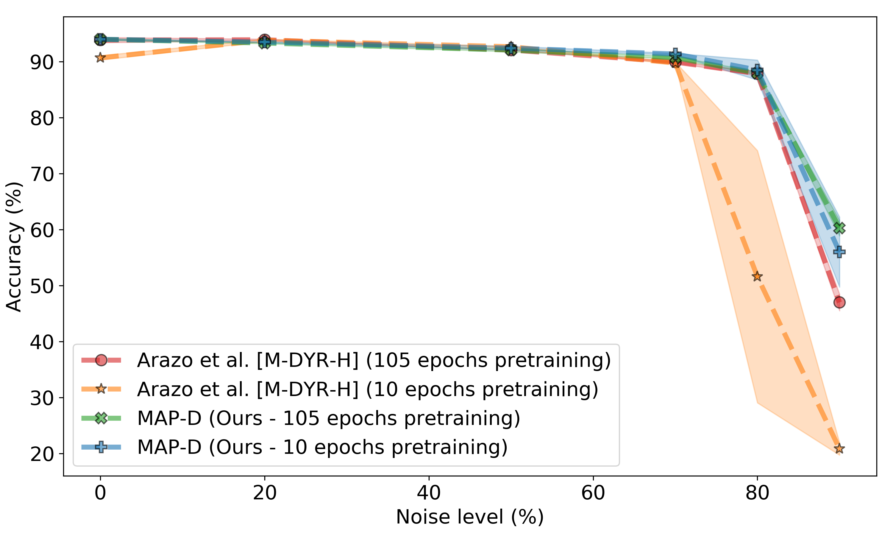
(a)

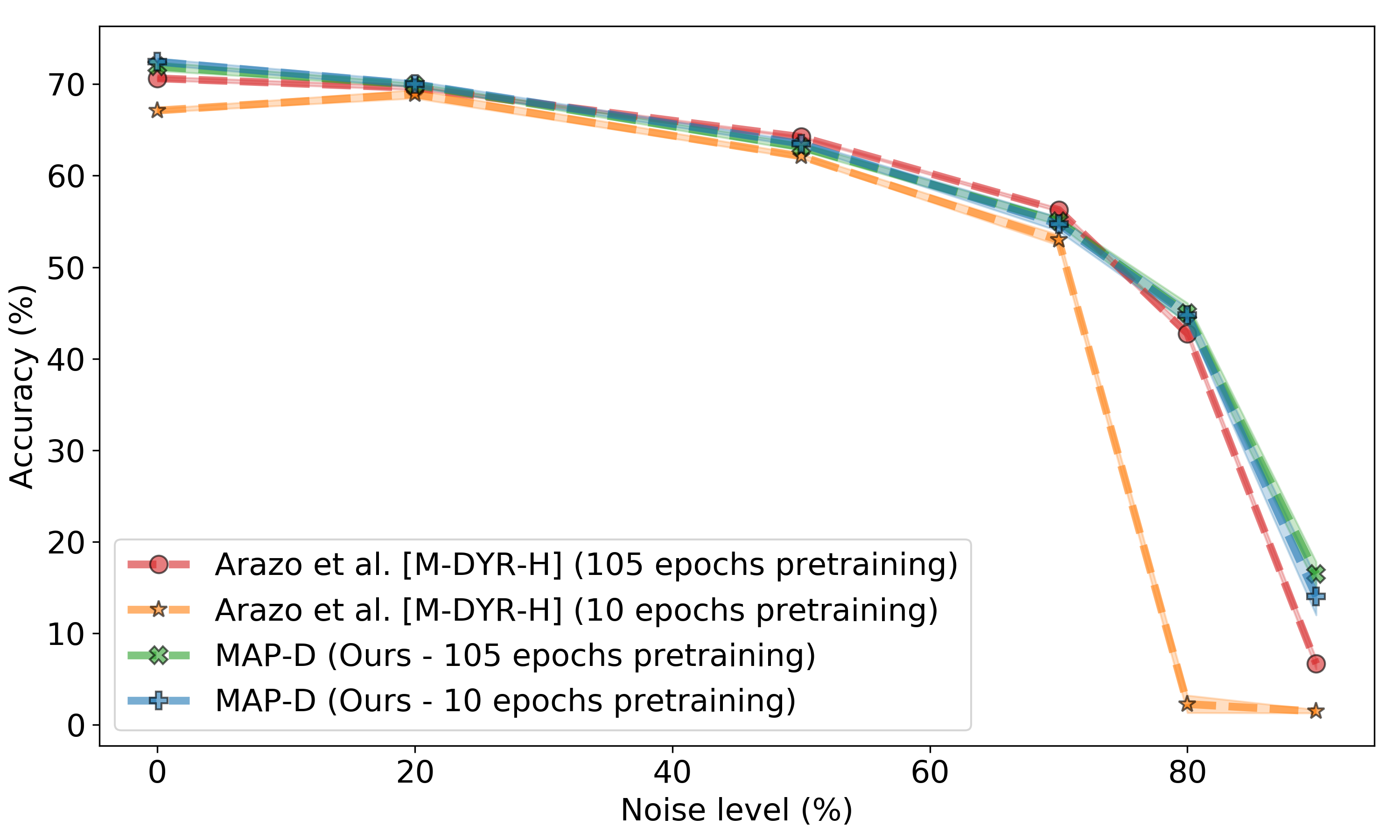
(b)

Figure 7: Comparison between pretraining schedules of 105 epochs (default value as set by Arazo et al. [5]) and 10 epochs. Mean and standard deviation reported over 3 random runs. MAP-D is robust against changes in the number of pretraining epochs, while the method in [5] achieves slightly poorer performance in the low-noise setting and significantly poorer performance in the high-noise setting.

3.4 Prioritized Training

Figure 8: Results for score-based prioritization with MAP-D (pink, lavender) compared against simple baselines. Mean and standard deviation computed over 3 random runs. The correct class score baselines (purple, orange) both select examples with the highest loss, which lead to poor performance due to label noise. Uniform selection baselines (blue, green) perform quite well, but take longer to train; out method achieves almost a 10x training speedup. RHO Loss* baseline (grey)) plots original results reported in [42] while all other results use our implementation. While * use a different reporting interval, results remain comparable. The two methods are similar in training speed, but MAP-D achieves higher accuracy.

Prioritized training refers to selection of most useful points for training in an online fashion with the aim of speeding up the training process. We consider the online batch selection scenario presented in [42], where we only train on a selected 10% of the examples in each minibatch. Simple baselines for this task include selecting points with high loss or at uniform random. It can be helpful to prioritize examples which are not yet learned (i.e. consistently correctly classified), but this can also select for mislabeled examples, which are common in large web-scraped datasets such as Clothing1M [69]. As noted by Mindermann et al. [42], we need to find points which are useful to learn. Applying MAP-D in this context allows us to leverage training dynamics to identify such examples - we look for examples that are not already learned, but which still have training dynamics that resemble clean data:

training_score = (clean_score + (1. - correct_class_confidence)) / 2. (9)

where clean_score is the probability of an example being clean (vs. noisy) according to the k-NN classifier described in Section 2.1.1. An example can achieve a maximum score of 1 under this metric when MAP-D predicts the example is clean, but the model assigns 0 probability to the correct label. Following Mindermann et al. [42], we select 32 examples from each minibatch of 320. For (class-)balanced sampling, we also ensure that we always select at least 2 examples from each of the 14 possible classes, which significantly improves performance. Figure 8 shows the effectiveness of this approach vs. these baselines; we achieve a 10x speedup over uniform random selection of examples.

We also report the original results from [42] for reference which uses a different reporting interval.  [42] requires pretraining a separate model, and uses the prediction of that model to decide which points to prioritize for training. Our method on the other hand uses an online MAP-D trajectory scheme to decide whether an example is clean or noisy. It is important to note that using balanced sampling with RHO Loss [42] is likely to also improve performance for [42].

3.5 Detection of Minority Group Samples

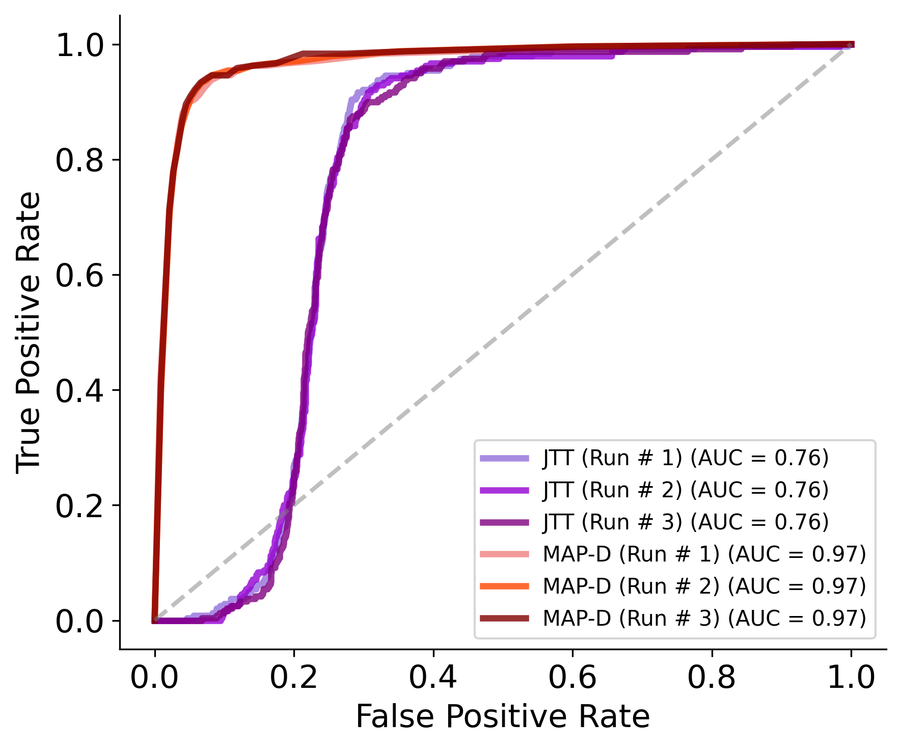
(a)

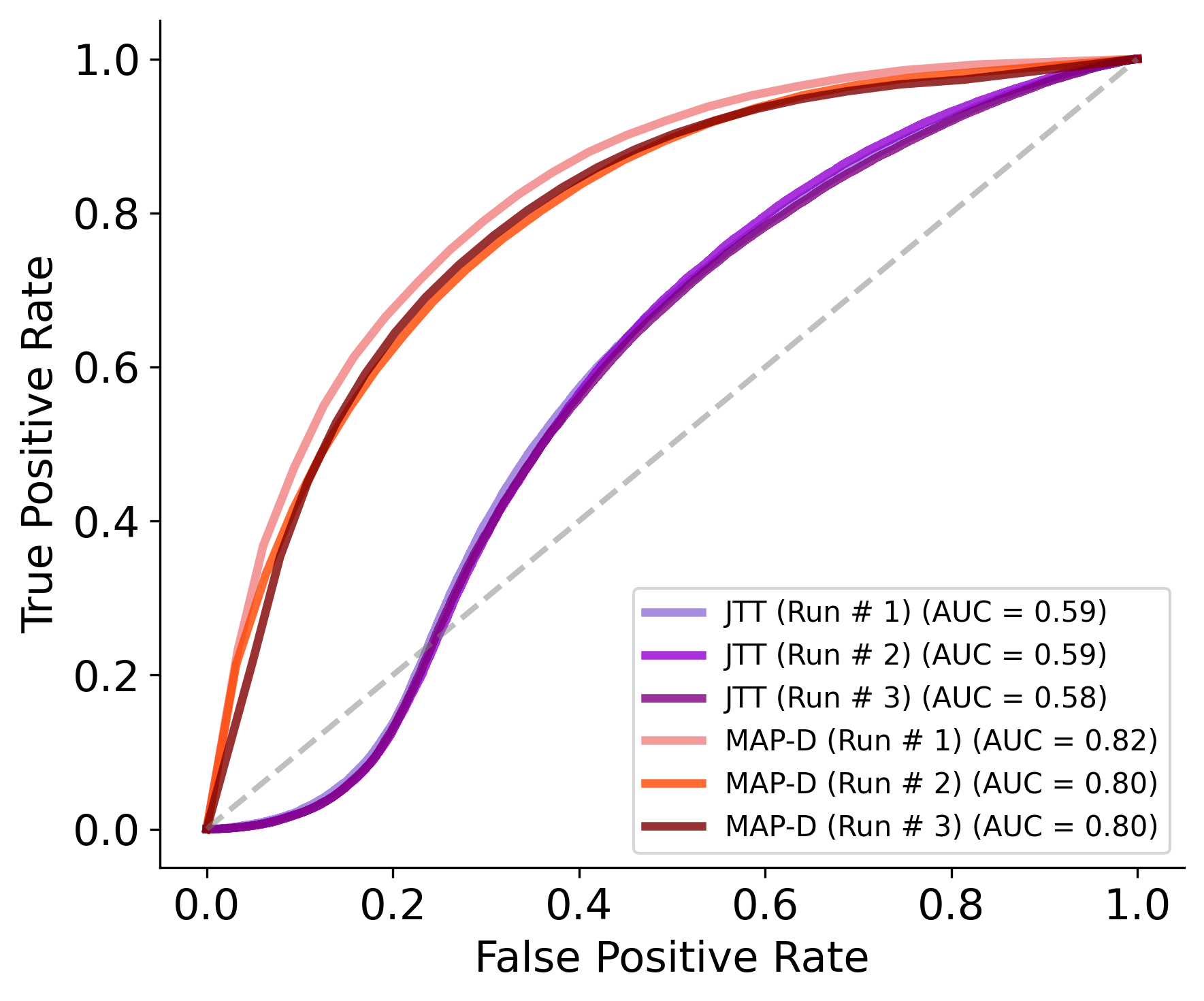
(b)

Figure 9: Demonstration of the effectiveness of MAP-D in detecting minority-group samples on two famous minority-group datasets with spurious correlations, compared to the detection performance of JTT [39] which relies on early-stopping. MAP-D achieves better or similar performance, without needing costly hyperparameter tuning or retraining.

Minimizing average-case error often hurts performance on minority sub-groups that might be present in a dataset [53, 54, 39]. For instance, models might learn to rely on spurious features that are only predictive for majority groups. Identifying minority-group samples can help detect and correct such issues, improving model fairness.

Previous works identify minority examples as those that are not already fit after some number of training epochs, and retrain from scratch with those examples upweighted [39, 75]. The number of epochs is treated as a hyperparameter; tuning it requires running the training process twice (without and then with upweighting) and evaluating on held-out known-to-be-minority examples. Instead of relying on the inductive bias that minority examples will be harder to fit, we apply MAP-D to find examples that match minority examples’ training dynamics, and find this is much more effective method of identifying minority examples, see Figure  9. This avoids the costly hyperparameter tuning required by previous methods. Instead of just using 250 examples per probe category, we use the complete validation set in this case to be consistent with prior work [39]. Furthermore, these examples are not included as part of the training set in order to match the statistics of examples at test time.

4 Related Work

Many research directions focus on properties of data and leveraging them in turn to improve the training process. We categorize and discuss each of these below.

Difficulty of examples

Koh and Liang [34] proposes influence functions to identify training points most influential on a given prediction. Work by Arpit et al. [6], Li et al. [38], Feldman [17], Feldman and Zhang [18] develop methods that measure the degree of memorization required of individual examples. While Jiang et al. [29] proposes a consistency score to rank each example by alignment with the training instances, Carlini et al. [11] considers several different measures to isolate prototypes that could conceivably be extended to rank the entire dataset. Agarwal et al. [2] leverage variance of gradients across training to rank examples by learning difficulty. Further, Hooker et al. [23] classify examples as challenging according to sensitivity to varying model capacity. In contrast to all these approaches that attempt to rank an example along one axis, MAP-D is able to discern between different sources of uncertainty without any significant computational cost by directly leveraging the training dynamics of the model.

Coreset selection techniques

The aim of these methods is to find prototypical examples that represent a larger corpus of data [74, 9, 32, 33], which can be used to speed up training [55, 56, 27] or aid in interpretability of the model predictions [72]. MAP-D provides a computationally feasible alternate to identify and surface these coresets.

Noisy examples

A special case of example difficulty is noisy labels, and correcting for their presence. Arazo et al. [5] use parameterized mixture models with two modes (for clean and noisy) fit to sample loss statistics, which they then use to relabel samples determined to be noisy. Li et al. [37] similarly uses mixture models to identify mislabelled samples, but actions on them by discarding the labels entirely and using these samples for auxiliary self-supervised training. These methods are unified by the goal of identifying examples that the model finds challenging, but unlike MAP-D, do not distinguish between the sources of this difficulty.

Leveraging training signal

There are several prior techniques that also leverage network training dynamics over distinct phases of learning [1, 29, 41, 16, 2]. Notably, Pleiss et al. [50] use loss dynamics of samples over the course of training, but calculate an Area-Under-Margin metric and show it can distinguish correct but difficult samples from mislabelled samples. In contrast, MAP-D is capable of inferring multiple data properties. Swayamdipta et al. (2020) [59] computed the mean and variance of the model’s confidence for the target label throughout training to identify interesting examples in the context of natural language processing. However, their method is limited in terms of identifying only easy, hard, or confusing examples. Our work builds upon this direction and can be extended to arbitrary sources of uncertainty based on defined probe suites leveraging loss trajectories.

Adaptive training

Adaptive training leverages training dynamics of the network to identify examples that are worth learning. Loss-based prioritization [28, 31] upweight high loss examples, assuming these examples are challenging yet learnable. These methods have been shown to quickly degrade in performance in the presence of even small amounts of noise since upweighting noisy samples hurts generalization [26, 49]. D’souza et al. [15] motivate using targeted data augmentation to distinguish between different sources of uncertainty, and adapting training based upon differences in rates of learning. On the other hand, several methods prioritize learning on examples with a low loss assuming that they are more meaningful to learn. Recent work has also attempted to discern between points that are learnable (not noisy), worth learning (in distribution), and not yet learned (not redundant) [42]. MAP-D can also be leveraged for adaptive training by defining the different sources of uncertainties of interest.

Minority group samples

The recent interest has been particularly towards finding and dealing with minority group samples to promote model fairness [53, 54, 39, 75, 43]. The dominant approach to deal with this problem without assuming access to group labels is to either pseudo-label the dataset using a classifier [43] or to train a model with early-stopping via a small validation set to surface minority group samples [39, 75]. However, this setting only works for the contrived datasets where the model can classify the group based on the background. MAP-D leverages the population statistics rather than exploiting the curation process of the dataset to naturally surface minority group samples, which is scalable and applicable in the real-world.

5 Conclusion

We introduce the problem of Metadata Archeology as the task of surfacing and inferring metadata of different examples in a dataset, noting that the relational qualities of metadata are of special interest (as compared to ordinary data features) for auditing, fairness, and many other applications. Metadata archaeology provides a unified framework for addressing multiple such data quality issues in large-scale datasets. We also propose a simple approach to this problem, Metadata Archaeology via Probe Dynamics (MAP-D), based on the assumption that examples with similar learning dynamics present the same metadata. We show that MAP-D is successful in identifying appropriate metadata features for data examples, even with no human labelling, making it a competitive approach for a variety of downstream tasks and datasets and a useful tool for auditing large scale datasets.

Limitations

This work is focused on a computer vision setting; we consider an important direction of future work to be extending this to other domains. MAP-D surfaces examples from the model based on the loss trajectories. This is based on a strong assumption that these loss trajectories are separable. It is possible that the learning curve for two set of probe categories exhibit similar behavior, limiting the model’s capacity in telling them apart. In this case, the learning curve is no longer a valid discriminator between probes. However, for good constructions of probe categories relying on global population statistics, we consider MAP-D to be a competitive and data-efficient method.

Appendix

Appendix A Experimental Details

In all experiments, we use variants of the ResNet architecture and leverage standard image classification datasets – CIFAR-10/100 and ImageNet. We train with SGD using standard hyperparameter settings: learning rate 0.1, momentum 0.9, weight-decay 0.0005, and a cosine learning rate decay. We achieve top-1 accuracies of 93.68% on CIFAR-10, 72.80% on CIFAR-100, and 73.94% on ImageNet.

CIFAR-10/100

To account for the smaller image size in this dataset, we follow standard practice and modify the models input layer to have stride 1 and filter size 3. We use a batch-size of 128 and train for 150 epochs. We use random horizontal flips and take a random crop of size $32\times 32$ after padding the image using reflection padding with a padding size of 4 [22]. For label noise correction experiments, we follow the experimental protocol of [5] with ResNet-18 where we train the model for 300 epochs with SGD and an initial learning rate of 0.1 decayed by a factor of 0.1 at the 100^th and 250^th epoch. A weight decay of 0.0001 is also applied.

ImageNet

We use a batch-size of 256 and train for 100 epochs. We apply center crop augmentation for testing as per the common practice (i.e. resize image to $256\times 256$ and take the center crop of size $224\times 224$)  [22, 45].

Waterbirds / CelebA

We use the same model architecture and hyperparameters as [39] in order to enable a fair and direct comparison. All experiments are based on the default ResNet-50 architecture. The Waterbirds models are trained for 300 epochs using SGD with an initial learning rate of 0.00001, and a high weight decay of 1.0. The model was early-stopped after the 60^th epoch for JTT [39]. The CelebA models are trained for 50 epochs using SGD with an initial learning rate of 0.00001, and a high weight decay of 0.1. The model was early-stopped after the first epoch for JTT [39].

Clothing1M

We use the online batch selection protocol from [42] where 32 examples are chosen from a large batch of 320 examples for training at each step. Following [42], we use AdamW optimizer with default hyperparameters as in PyTorch [47] and ImageNet pretrained ResNet-50. No learning rate decay is applied in this case.

Appendix B Probe suites for CIFAR-100

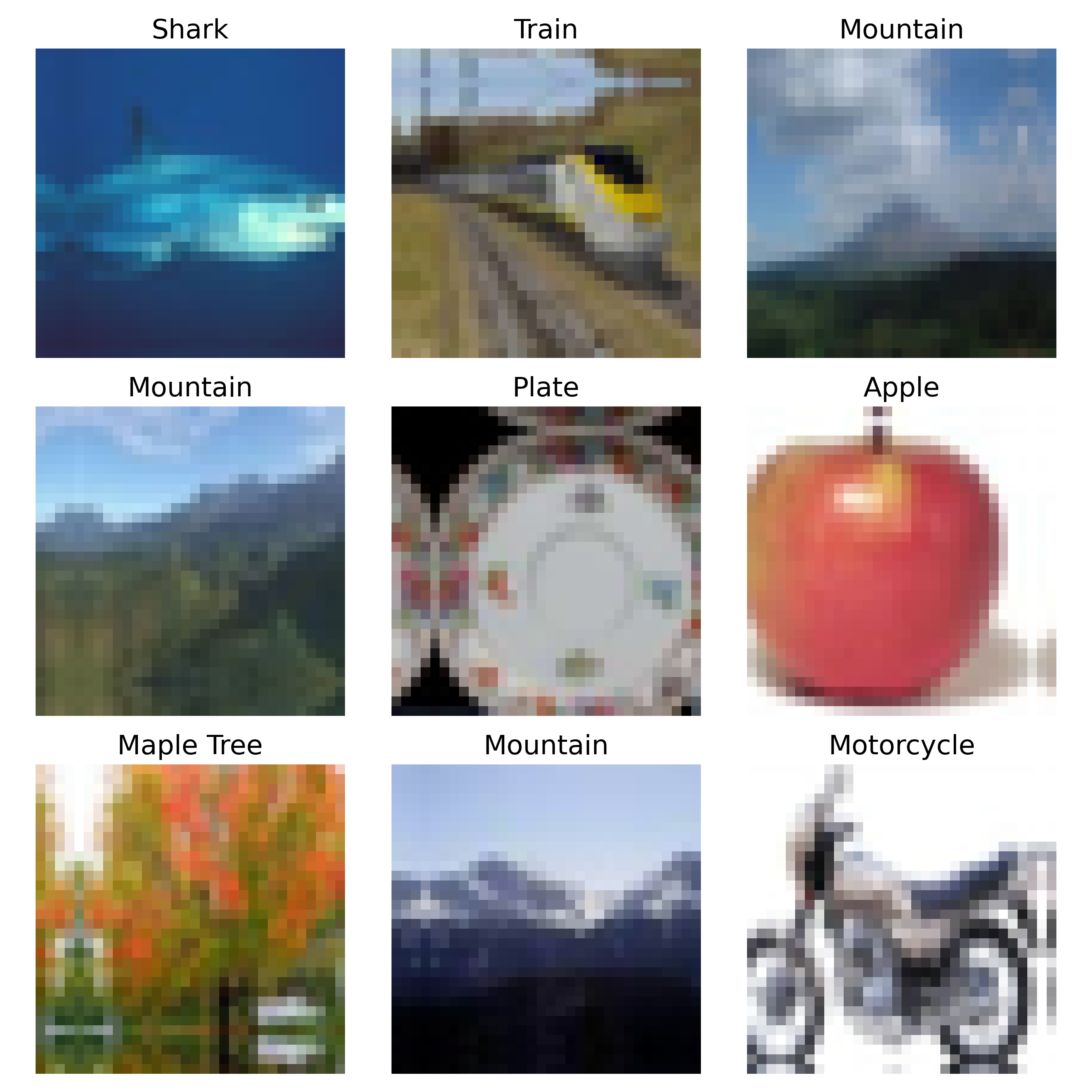
(a)

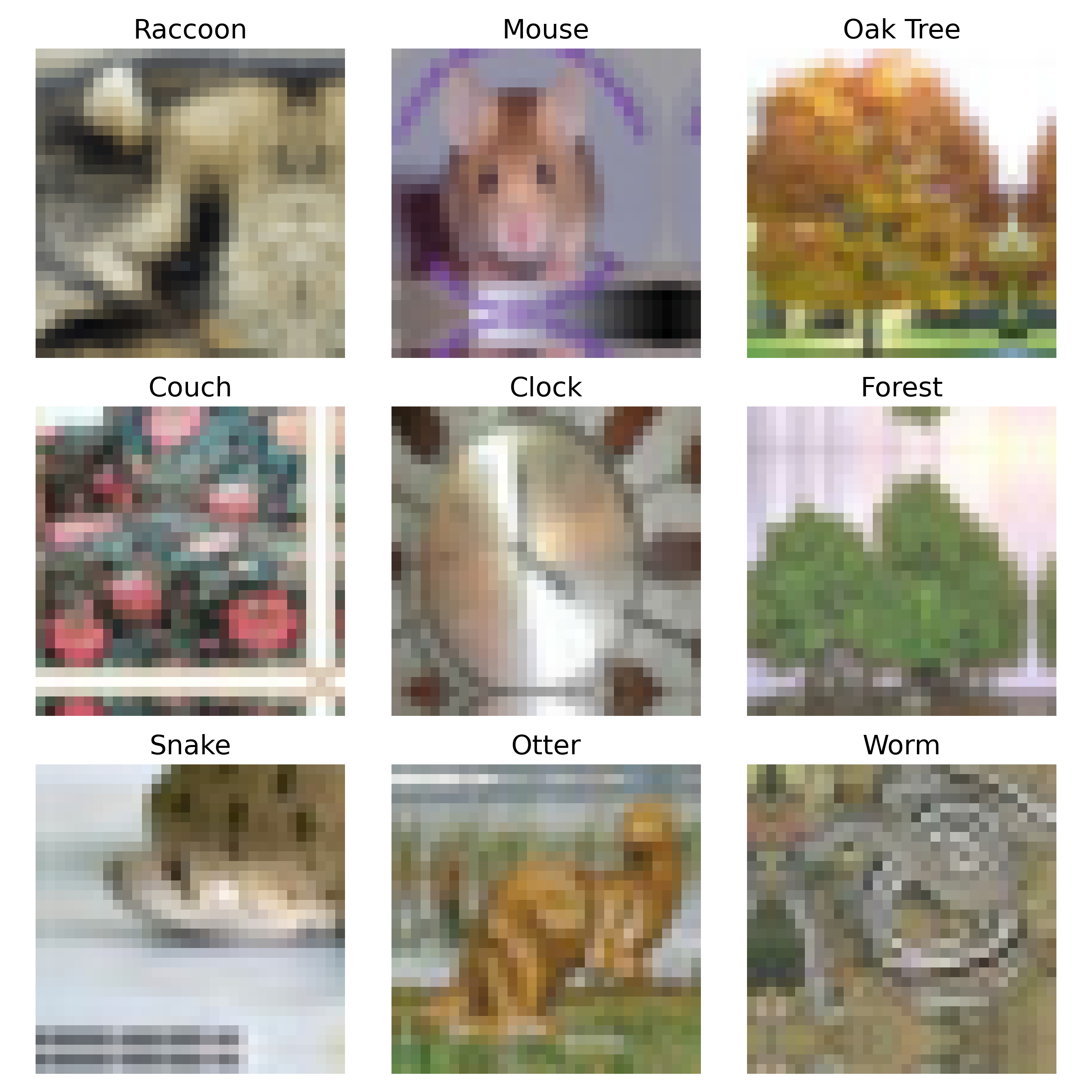
(b)

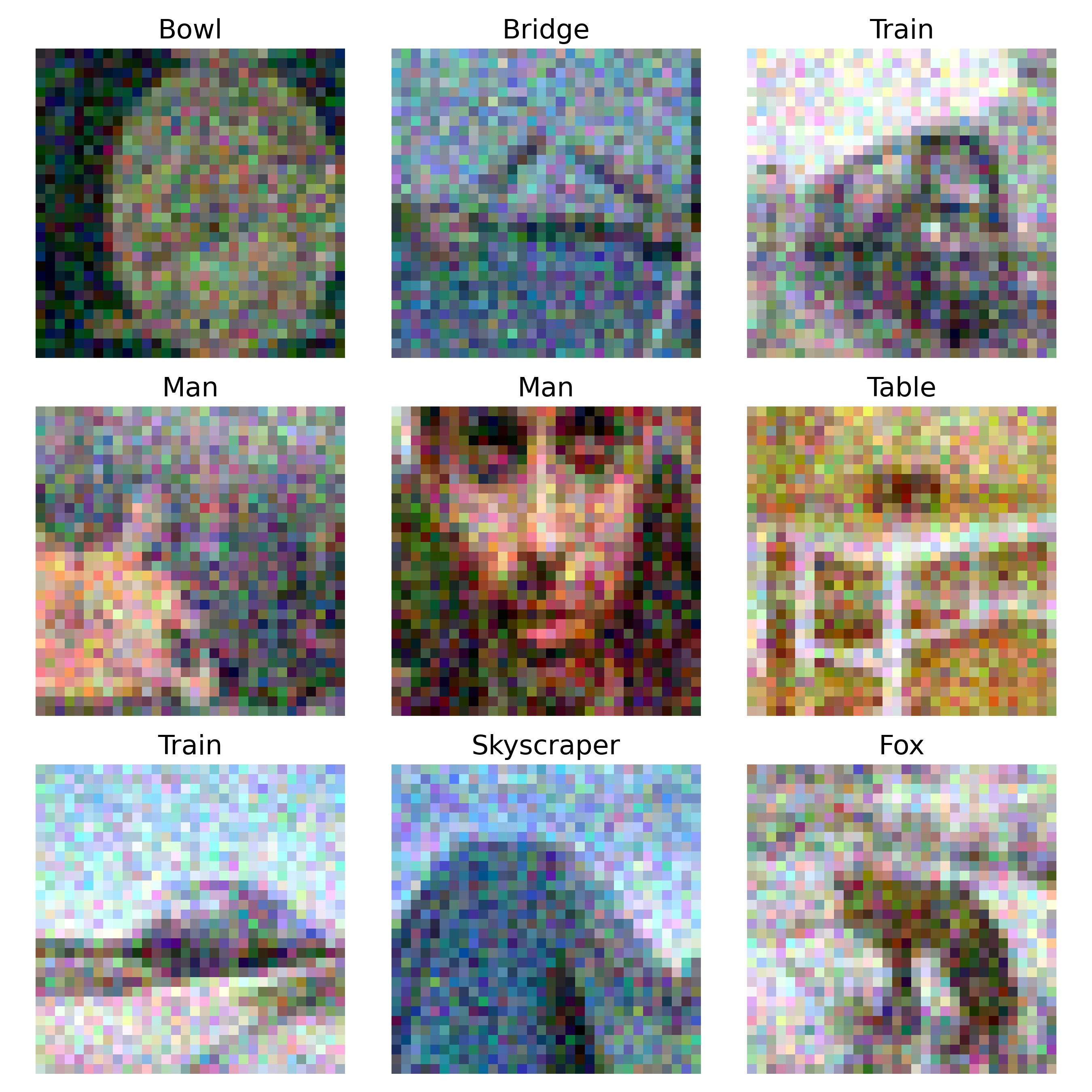
(c)

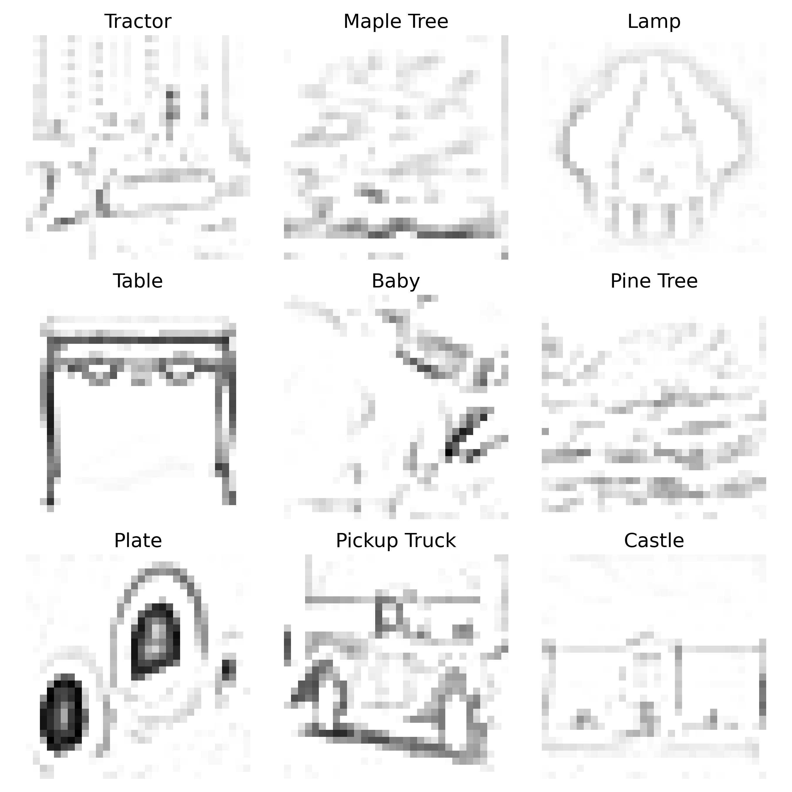
(d)

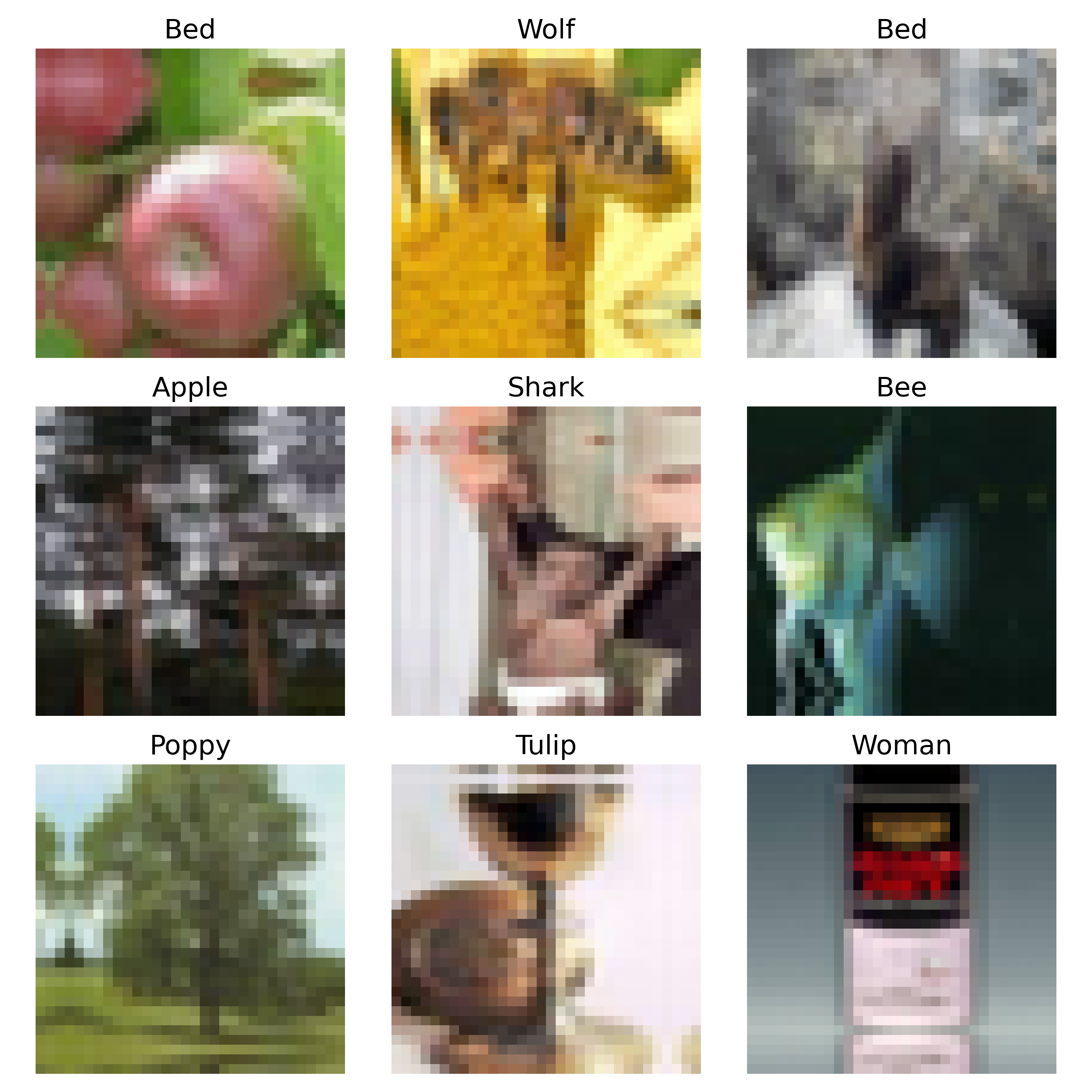
(e)

(f)

Figure 10: An example of the different kind of probes that can be defined on the CIFAR-100 dataset.

We present examples from the curated probe suites on CIFAR-100 in Fig. 10.

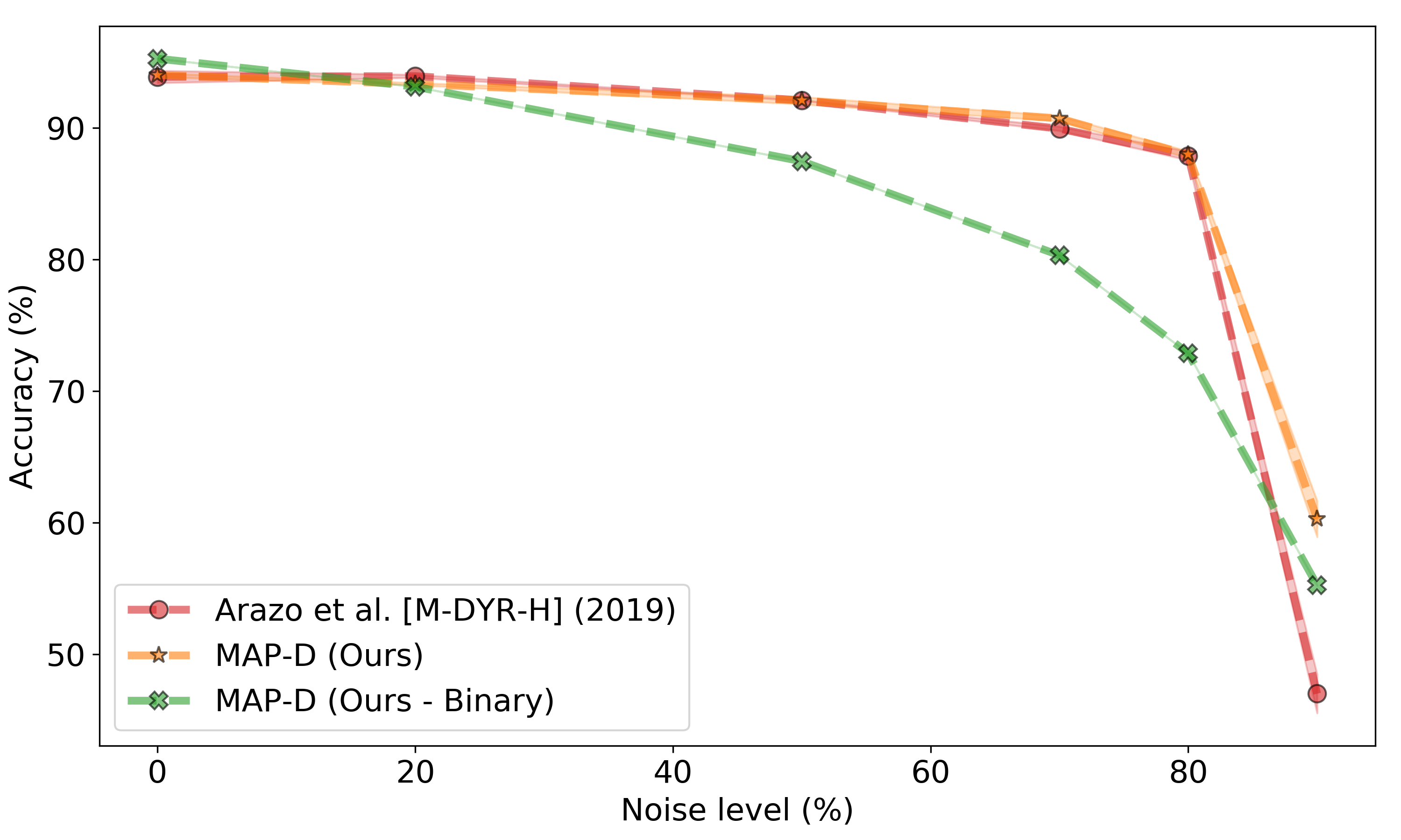
Figure 11: Ablation for label correction on CIFAR-10, where we use a binary prediction instead of probability estimates returned by MAP-D. This highlights the utility and effectiveness of the uncertainty estimates computed by MAP-D.

Appendix C Binary vs. Probabilistic Outputs in Label Correction

Arazo et al. (2019) [5] used a convex combination of the labels weighted by the actual probability returned by their BMM model. As MAP-D returns probability estimates, this enabled leveraging label correction framework in the same way. However, the utility of the uncertainty estimates is not immediately apparent. Therefore, in order to gauge the utility of these uncertainty estimates, we used binary predictions (argmax) instead of the actual probabilities returned by MAP-D. The results are visualized in Fig. 11. It is clear from the figure that the model struggles significantly in coping with noise when being restricted to binary predictions, indicating that the uncertainty estimates provided by MAP-D enables the model to learn the correct label.

References

- Achille et al. [2017] A. Achille, M. Rovere, and S. Soatto. Critical Learning Periods in Deep Neural Networks. ArXiv, abs/1711.08856, 2017.
- Agarwal et al. [2021] C. Agarwal, D. D’souza, and S. Hooker. Estimating Example Difficulty Using Variance of Gradients, 2021.
- Ahia et al. [2021] O. Ahia, J. Kreutzer, and S. Hooker. The Low-Resource Double Bind: An Empirical Study of Pruning for Low-Resource Machine Translation. In Findings of the Association for Computational Linguistics: EMNLP 2021, pages 3316–3333, Punta Cana, Dominican Republic, Nov. 2021. Association for Computational Linguistics. doi: 10.18653/v1/2021.findings-emnlp.282. URL https://aclanthology.org/2021.findings-emnlp.282.
- Andrus et al. [2021] M. Andrus, E. Spitzer, J. Brown, and A. Xiang. What We Can’t Measure, We Can’t Understand: Challenges to Demographic Data Procurement in the Pursuit of Fairness. In Proceedings of the 2021 ACM Conference on Fairness, Accountability, and Transparency, FAccT ’21, page 249–260, New York, NY, USA, 2021. Association for Computing Machinery. ISBN 9781450383097. doi: 10.1145/3442188.3445888. URL https://doi.org/10.1145/3442188.3445888.
- Arazo et al. [2019] E. Arazo, D. Ortego, P. Albert, N. O’Connor, and K. McGuinness. Unsupervised label noise modeling and loss correction. In International Conference on Machine Learning, pages 312–321. PMLR, 2019.
- Arpit et al. [2017] D. Arpit, S. Jastrzebski, N. Ballas, D. Krueger, E. Bengio, M. S. Kanwal, T. Maharaj, A. Fischer, A. Courville, Y. Bengio, et al. A closer look at memorization in deep networks. In International Conference on Machine Learning, pages 233–242. PMLR, 2017.
- Badgeley et al. [2019] M. Badgeley, J. Zech, L. Oakden-Rayner, B. Glicksberg, M. Liu, W. Gale, M. McConnell, B. Percha, and T. Snyder. Deep learning predicts hip fracture using confounding patient and healthcare variables. npj Digital Medicine, 2:31, 04 2019. doi: 10.1038/s41746-019-0105-1.
- Baldock et al. [2021] R. J. N. Baldock, H. Maennel, and B. Neyshabur. Deep Learning Through the Lens of Example Difficulty. In NeurIPS, 2021.
- Bien and Tibshirani [2012] J. Bien and R. Tibshirani. Prototype selection for interpretable classification. arXiv e-prints, art. arXiv:1202.5933, Feb. 2012.
- Buolamwini and Gebru [2018] J. Buolamwini and T. Gebru. Gender Shades: Intersectional Accuracy Disparities in Commercial Gender Classification. In S. A. Friedler and C. Wilson, editors, Proceedings of the 1st Conference on Fairness, Accountability and Transparency, volume 81 of Proceedings of Machine Learning Research, pages 77–91, New York, NY, USA, 23–24 Feb 2018. PMLR. URL http://proceedings.mlr.press/v81/buolamwini18a.html.
- Carlini et al. [2019] N. Carlini, Ú. Erlingsson, and N. Papernot. Distribution Density, Tails, and Outliers in Machine Learning: Metrics and Applications. arXiv e-prints, art. arXiv:1910.13427, Oct. 2019.
- Carlini et al. [2022] N. Carlini, D. Ippolito, M. Jagielski, K. Lee, F. Tramer, and C. Zhang. Quantifying Memorization Across Neural Language Models, 2022. URL https://arxiv.org/abs/2202.07646.
- Dastin [2018] J. Dastin. Amazon scraps secret AI recruiting tool that showed bias against women. Reuters, 2018. URL https://reut.rs/2p0ZWqe.
- Deng et al. [2009] J. Deng, W. Dong, R. Socher, L.-J. Li, K. Li, and L. Fei-Fei. ImageNet: A Large-Scale Hierarchical Image Database. In CVPR09, 2009.
- D’souza et al. [2021] D. D’souza, Z. Nussbaum, C. Agarwal, and S. Hooker. A tale of two long tails, 2021. URL https://arxiv.org/abs/2107.13098.
- Faghri et al. [2020] F. Faghri, D. Duvenaud, D. J. Fleet, and J. Ba. A Study of Gradient Variance in Deep Learning. arXiv e-prints, art. arXiv:2007.04532, July 2020.
- Feldman [2019] V. Feldman. Does learning require memorization? A short tale about a long tail. arXiv preprint arXiv:1906.05271, 2019.
- Feldman and Zhang [2020] V. Feldman and C. Zhang. What neural networks memorize and why: Discovering the long tail via influence estimation. arXiv preprint arXiv:2008.03703, 2020.
- Gruetzemacher et al. [2018] R. Gruetzemacher, A. Gupta, and D. B. Paradice. 3D deep learning for detecting pulmonary nodules in CT scans. Journal of the American Medical Informatics Association : JAMIA, 25 10:1301–1310, 2018.
- Harwell [2019] D. Harwell. A face-scanning algorithm increasingly decides whether you deserve the job. The Washington Post, 2019. URL https://wapo.st/2X3bupO.
- Hashimoto et al. [2018] T. Hashimoto, M. Srivastava, H. Namkoong, and P. Liang. Fairness Without Demographics in Repeated Loss Minimization. In J. Dy and A. Krause, editors, Proceedings of the 35th International Conference on Machine Learning, volume 80 of Proceedings of Machine Learning Research, pages 1929–1938, Stockholmsmässan, Stockholm Sweden, 10–15 Jul 2018. PMLR. URL http://proceedings.mlr.press/v80/hashimoto18a.html.
- He et al. [2016] K. He, X. Zhang, S. Ren, and J. Sun. Deep residual learning for image recognition. In Proceedings of the IEEE conference on computer vision and pattern recognition, pages 770–778, 2016.
- Hooker et al. [2019a] S. Hooker, A. Courville, G. Clark, Y. Dauphin, and A. Frome. What Do Compressed Deep Neural Networks Forget? arXiv e-prints, art. arXiv:1911.05248, Nov. 2019a.
- Hooker et al. [2019b] S. Hooker, A. Courville, G. Clark, Y. Dauphin, and A. Frome. What Do Compressed Deep Neural Networks Forget?, Nov. 2019b. URL https://arxiv.org/abs/1911.05248.
- Hooker et al. [2020] S. Hooker, N. Moorosi, G. Clark, S. Bengio, and E. Denton. Characterising Bias in Compressed Models, 2020.
- Hu et al. [2021] N. T. Hu, X. Hu, R. Liu, S. Hooker, and J. Yosinski. When does loss-based prioritization fail?, 2021.
- Huggins et al. [2017] J. H. Huggins, T. Campbell, and T. Broderick. Coresets for Scalable Bayesian Logistic Regression, 2017.
- Jiang et al. [2019] A. H. Jiang, D. L. K. Wong, G. Zhou, D. G. Andersen, J. Dean, G. R. Ganger, G. Joshi, M. Kaminksy, M. Kozuch, Z. C. Lipton, and P. Pillai. Accelerating deep learning by focusing on the biggest losers, 2019. URL https://arxiv.org/abs/1910.00762.
- Jiang et al. [2020] Z. Jiang, C. Zhang, K. Talwar, and M. C. Mozer. Characterizing Structural Regularities of Labeled Data in Overparameterized Models. arXiv e-prints, art. arXiv:2002.03206, Feb. 2020.
- Kaplan et al. [2020] J. Kaplan, S. McCandlish, T. Henighan, T. B. Brown, B. Chess, R. Child, S. Gray, A. Radford, J. Wu, and D. Amodei. Scaling laws for neural language models. CoRR, abs/2001.08361, 2020. URL https://arxiv.org/abs/2001.08361.
- Katharopoulos and Fleuret [2018] A. Katharopoulos and F. Fleuret. Not all samples are created equal: Deep learning with importance sampling, 2018. URL https://arxiv.org/abs/1803.00942.
- Kim et al. [2015] B. Kim, C. Rudin, and J. Shah. The Bayesian Case Model: A Generative Approach for Case-Based Reasoning and Prototype Classification. arXiv e-prints, art. arXiv:1503.01161, Mar. 2015.
- Kim et al. [2016] B. Kim, R. Khanna, and O. O. Koyejo. Examples are not enough, learn to criticize! Criticism for Interpretability. In D. D. Lee, M. Sugiyama, U. V. Luxburg, I. Guyon, and R. Garnett, editors, Advances in Neural Information Processing Systems 29, pages 2280–2288. Curran Associates, Inc., 2016. URL http://papers.nips.cc/paper/6300-examples-are-not-enough-learn-to-criticize-criticism-for-interpretability.pdf.
- Koh and Liang [2017] P. W. Koh and P. Liang. Understanding Black-box Predictions via Influence Functions. arXiv e-prints, art. arXiv:1703.04730, Mar. 2017.
- Krizhevsky et al. [2009] A. Krizhevsky, G. Hinton, et al. Learning multiple layers of features from tiny images. 2009.
- LeBrun et al. [2022] B. LeBrun, A. Sordoni, and T. J. O’Donnell. Evaluating Distributional Distortion in Neural Language Modeling. ArXiv, abs/2203.12788, 2022.
- Li et al. [2020a] J. Li, R. Socher, and S. C. Hoi. Dividemix: Learning with noisy labels as semi-supervised learning. arXiv preprint arXiv:2002.07394, 2020a.
- Li et al. [2020b] M. Li, M. Soltanolkotabi, and S. Oymak. Gradient descent with early stopping is provably robust to label noise for overparameterized neural networks. In International Conference on Artificial Intelligence and Statistics, pages 4313–4324. PMLR, 2020b.
- Liu et al. [2021] E. Z. Liu, B. Haghgoo, A. S. Chen, A. Raghunathan, P. W. Koh, S. Sagawa, P. Liang, and C. Finn. Just train twice: Improving group robustness without training group information. In International Conference on Machine Learning, pages 6781–6792. PMLR, 2021.
- Liu et al. [2015] Z. Liu, P. Luo, X. Wang, and X. Tang. Deep Learning Face Attributes in the Wild. In Proceedings of International Conference on Computer Vision (ICCV), December 2015.
- Mangalam and Prabhu [2019] K. Mangalam and V. U. Prabhu. Do deep neural networks learn shallow learnable examples first. In Workshop on Identifying and Understanding Deep Learning Phenomena at 36th International Conference on Machine Learning, 2019.
- Mindermann et al. [2022] S. Mindermann, J. Brauner, M. Razzak, M. Sharma, A. Kirsch, W. Xu, B. Höltgen, A. N. Gomez, A. Morisot, S. Farquhar, et al. Prioritized training on points that are learnable, worth learning, and not yet learnt. arXiv preprint arXiv:2206.07137, 2022.
- Nam et al. [2022] J. Nam, J. Kim, J. Lee, and J. Shin. Spread spurious attribute: Improving worst-group accuracy with spurious attribute estimation. arXiv preprint arXiv:2204.02070, 2022.
- NHTSA [2017] NHTSA. Technical report, U.S. Department of Transportation, National Highway Traffic, Tesla Crash Preliminary Evaluation Report Safety Administration. PE 16-007, Jan 2017.
- NVIDIA [2022] NVIDIA. ResNet v1.5 for pytorch: Nvidia NGC, 2022. URL https://catalog.ngc.nvidia.com/orgs/nvidia/resources/resnet_50_v1_5_for_pytorch.
- Oakden-Rayner et al. [2019] L. Oakden-Rayner, J. Dunnmon, G. Carneiro, and C. Ré. Hidden Stratification Causes Clinically Meaningful Failures in Machine Learning for Medical Imaging. arXiv e-prints, art. arXiv:1909.12475, Sep 2019.
- Paszke et al. [2019] A. Paszke, S. Gross, F. Massa, A. Lerer, J. Bradbury, G. Chanan, T. Killeen, Z. Lin, N. Gimelshein, L. Antiga, et al. Pytorch: An imperative style, high-performance deep learning library. Advances in neural information processing systems, 32, 2019.
- Patrini et al. [2017] G. Patrini, A. Rozza, A. Krishna Menon, R. Nock, and L. Qu. Making deep neural networks robust to label noise: A loss correction approach. In Proceedings of the IEEE conference on computer vision and pattern recognition, pages 1944–1952, 2017.
- Paul et al. [2021] M. Paul, S. Ganguli, and G. K. Dziugaite. Deep Learning on a Data Diet: Finding Important Examples Early in Training, 2021.
- Pleiss et al. [2020] G. Pleiss, T. Zhang, E. Elenberg, and K. Q. Weinberger. Identifying mislabeled data using the area under the margin ranking. Advances in Neural Information Processing Systems, 33:17044–17056, 2020.
- Reed et al. [2014] S. Reed, H. Lee, D. Anguelov, C. Szegedy, D. Erhan, and A. Rabinovich. Training deep neural networks on noisy labels with bootstrapping. arXiv preprint arXiv:1412.6596, 2014.
- Roberts et al. [2020] A. Roberts, C. Raffel, and N. Shazeer. How Much Knowledge Can You Pack Into the Parameters of a Language Model? CoRR, abs/2002.08910, 2020. URL https://arxiv.org/abs/2002.08910.
- Sagawa et al. [2019] S. Sagawa, P. W. Koh, T. B. Hashimoto, and P. Liang. Distributionally robust neural networks for group shifts: On the importance of regularization for worst-case generalization. arXiv preprint arXiv:1911.08731, 2019.
- Sagawa et al. [2020] S. Sagawa, A. Raghunathan, P. W. Koh, and P. Liang. An investigation of why overparameterization exacerbates spurious correlations. In International Conference on Machine Learning, pages 8346–8356. PMLR, 2020.
- Sener and Savarese [2018] O. Sener and S. Savarese. Active Learning for Convolutional Neural Networks: A Core-Set Approach, 2018.
- Shim et al. [2021] J. Shim, K. Kong, and S.-J. Kang. Core-set Sampling for Efficient Neural Architecture Search. In e ICML 2021 Workshop on Subset Selection in ML, 2021.
- Shmueli et al. [2021] B. Shmueli, J. Fell, S. Ray, and L.-W. Ku. Beyond fair pay: Ethical implications of nlp crowdsourcing. ArXiv, abs/2104.10097, 2021.
- Steiger et al. [2021] M. Steiger, T. J. Bharucha, S. Venkatagiri, M. J. Riedl, and M. Lease. The psychological well-being of content moderators: The emotional labor of commercial moderation and avenues for improving support. Proceedings of the 2021 CHI Conference on Human Factors in Computing Systems, 2021.
- Swayamdipta et al. [2020] S. Swayamdipta, R. Schwartz, N. Lourie, Y. Wang, H. Hajishirzi, N. A. Smith, and Y. Choi. Dataset cartography: Mapping and diagnosing datasets with training dynamics. arXiv preprint arXiv:2009.10795, 2020.
- Słowik and Bottou [2021] A. Słowik and L. Bottou. Algorithmic Bias and Data Bias: Understanding the Relation between Distributionally Robust Optimization and Data Curation. ArXiv, abs/2106.09467, 2021.
- Talukdar et al. [2021] A. Talukdar, M. Dagar, P. Gupta, and V. Menon. Training dynamic based data filtering may not work for NLP datasets. In Proceedings of the Fourth BlackboxNLP Workshop on Analyzing and Interpreting Neural Networks for NLP, pages 296–302, Punta Cana, Dominican Republic, Nov. 2021. Association for Computational Linguistics. doi: 10.18653/v1/2021.blackboxnlp-1.22. URL https://aclanthology.org/2021.blackboxnlp-1.22.
- Thulasidasan et al. [2019a] S. Thulasidasan, T. Bhattacharya, J. Bilmes, G. Chennupati, and J. Mohd-Yusof. Combating Label Noise in Deep Learning using Abstention. In K. Chaudhuri and R. Salakhutdinov, editors, Proceedings of the 36th International Conference on Machine Learning, volume 97 of Proceedings of Machine Learning Research, pages 6234–6243. PMLR, 09–15 Jun 2019a. URL http://proceedings.mlr.press/v97/thulasidasan19a.html.
- Thulasidasan et al. [2019b] S. Thulasidasan, T. Bhattacharya, J. A. Bilmes, G. Chennupati, and J. Mohd-Yusof. Combating Label Noise in Deep Learning Using Abstention. In ICML, 2019b.
- Vasudevan et al. [2022] V. Vasudevan, B. Caine, R. Gontijo-Lopes, S. Fridovich-Keil, and R. Roelofs. When does dough become a bagel? Analyzing the remaining mistakes on ImageNet, 2022. URL https://arxiv.org/abs/2205.04596.
- Veale and Binns [2017] M. Veale and R. Binns. Fairer machine learning in the real world: Mitigating discrimination without collecting sensitive data. Big Data & Society, 4(2):2053951717743530, 2017. doi: 10.1177/2053951717743530. URL https://doi.org/10.1177/2053951717743530.
- Wang et al. [2018] Y. Wang, W. Liu, X. Ma, J. Bailey, H. Zha, L. Song, and S. Xia. Iterative learning with open-set noisy labels. 2018 IEEE/CVF Conference on Computer Vision and Pattern Recognition, pages 8688–8696, 2018.
- Wei et al. [2022] J. Wei, Y. Tay, R. Bommasani, C. Raffel, B. Zoph, S. Borgeaud, D. Yogatama, M. Bosma, D. Zhou, D. Metzler, E. H. Chi, T. Hashimoto, O. Vinyals, P. Liang, J. Dean, and W. Fedus. Emergent abilities of large language models, 2022. URL https://arxiv.org/abs/2206.07682.
- Wu et al. [2020] P. Wu, S. Zheng, M. Goswami, D. Metaxas, and C. Chen. A Topological Filter for Learning with Label Noise, 2020.
- Xiao et al. [2015] T. Xiao, T. Xia, Y. Yang, C. Huang, and X. Wang. Learning from massive noisy labeled data for image classification. In CVPR, 2015.
- Xie et al. [2019] H. Xie, D. Yang, N. Sun, Z. Chen, and Y. Zhang. Automated pulmonary nodule detection in CT images using deep convolutional neural networks. Pattern Recognition, 85:109–119, 2019. ISSN 0031-3203. doi: https://doi.org/10.1016/j.patcog.2018.07.031. URL http://www.sciencedirect.com/science/article/pii/S0031320318302711.
- Yi and Wu [2019] K. Yi and J. Wu. Probabilistic End-to-end Noise Correction for Learning with Noisy Labels, 2019.
- Yoon et al. [2019] J. Yoon, S. O. Arik, and T. Pfister. RL-LIM: Reinforcement Learning-based Locally Interpretable Modeling, 2019.
- Zhang et al. [2017] H. Zhang, M. Cisse, Y. N. Dauphin, and D. Lopez-Paz. mixup: Beyond empirical risk minimization. arXiv preprint arXiv:1710.09412, 2017.
- Zhang [1992] J. Zhang. Selecting Typical Instances in Instance-Based Learning. In D. Sleeman and P. Edwards, editors, Machine Learning Proceedings 1992, pages 470–479. Morgan Kaufmann, San Francisco (CA), 1992. ISBN 978-1-55860-247-2. doi: https://doi.org/10.1016/B978-1-55860-247-2.50066-8. URL http://www.sciencedirect.com/science/article/pii/B9781558602472500668.
- Zhang et al. [2022] M. Zhang, N. S. Sohoni, H. R. Zhang, C. Finn, and C. Ré. Correct-n-contrast: A contrastive approach for improving robustness to spurious correlations. arXiv preprint arXiv:2203.01517, 2022.