ALMA Datacubes and Continuum Maps of the Irradiated Western Wall in Carina

Abstract

We present ALMA observations of the continuum and line emission of ¹²CO, ¹³CO, C¹⁸O, and [C I] for a portion of the G287.38-0.62 (Car 1-E) region in the Carina star-forming complex. The new data record how a molecular cloud responds on subarcsecond scales when subjected to a powerful radiation front, and provide insights into the overall process of star formation within regions that contain the most massive young stars. The maps show several molecular clouds superpose upon the line of sight, including a portion of the Western Wall, a highly-irradiated cloud situated near the young star cluster Trumpler 14. In agreement with theory, there is a clear progression from fluoresced H₂, to [C I], to C¹⁸O with distance into the PDR front. Emission from optically thick ¹²CO extends across the region, while ¹³CO, [C I] and especially C¹⁸O are more optically thin, and concentrate into clumps and filaments closer to the PDR interface. Within the Western Wall cloud itself we identify 254 distinct core-sized clumps in our datacube of C¹⁸O. The mass distribution of these objects is similar to that of the stellar IMF. Aside from a large-scale velocity gradient, the clump radial velocities lack any spatial coherence size. There is no direct evidence for triggering of star formation in the Western Wall in that its C¹⁸O clumps and continuum cores appear starless, with no pillars present. However, the densest portion of the cloud lies closest to the PDR, and the C¹⁸O emission is flattened along the radiation front.

1 Introduction

The first surveys of molecular clouds established that the densest portions of the clouds, known as cores, mark locations where stars are born (e.g. Myers & Benson, 1983). These observations make sense from a theoretical standpoint, as the densest parts of the cloud should be the first areas to collapse gravitationally, and numerical models predict that within quiescent regions core collapse should begin within its inner regions and then expand outward (e.g. Shu, 1977; Shu et al., 1987). As material accumulates, the central density and temperature of the core should rise until a protostar forms, and the object subsequently evolves along an evolutionary track in the HR-diagram determined primarily by its mass.

The decades since these early studies have witnessed an avalanche of new data related to star formation as space-based missions such as IRAS, Spitzer, Herschel, and WISE have surveyed the galactic plane across the entire infrared and far-infrared spectral bandpasses, while targeted ground-based studies in both continuum and various molecular emission lines provided deep maps with high spatial resolution of the dust distribution, molecular content, and dynamics within individual star-forming regions. Although the general scenario that stars form in molecular cloud cores remains intact, the new observations have made it clear that the actual process of star formation can be incredibly complex. In many and perhaps most regions, the factors behind this complexity seem to play a dominant role in determining whether or not a star forms at all, and also influence the masses, compositions, and orbital radii of planets that coalesce out of the protostellar disk material remaining after the star forms.

One of the main contributing factors to the complexity in star formation regions is simply the lack of spherical symmetry within molecular clouds. Recent parsec-scale maps with Herschel have shown that dust in molecular clouds appears highly filamentary (Hill et al., 2011; Arzoumanian et al., 2011), and velocity maps along these filaments display large-scale organized motions (Peretto et al., 2014; Kong et al., 2019), clearly demonstrating that simple 1-dimensional models of collapse do not represent the physics accurately. Polarization maps sometimes indicate ordered magnetic fields on large scales that could affect the dynamics, while other regions appear more chaotic and turbulent (Planck Collab., 2016; Hull et al., 2020). High-resolution maps of molecular clouds now available with ALMA also show geometrical complexity on small-scales ($\lesssim$ 0.01 pc Tokuda et al., 2020), where ambipolar diffusion is important to consider when assessing magnetic pressure support for collapsing cores (Chen & Ostriker, 2014). The additional physics introduced by these processes affects the efficiency of star formation within a cloud as well as the time scale for collapse. Geometrical factors are particularly important for massive stars, as cavities created along the rotation axes provide a means for radiation to escape while accretion is ongoing through a disk, without which it would be impossible to accumulate enough material to create the highest mass stars (Rosen et al., 2016; Krumholz et al., 2005).

Once stars form, the situation becomes even more complex because radiation from the newborn stars and collimated bipolar outflows deposit energy back into the surrounding cloud. This energy could cause the gas in the nascent cloud to disperse or drive turbulence into the cloud that adds a pressure term to counter gravitational collapse, effectively lowering the star formation rate. On the other hand, shock waves from outflows and radiation fronts also cause density enhancements, which in turn might trigger stars to form by pushing pre-existing clumps past their Jeans limit (e.g. Haworth et al., 2011). On large scales, because there is a finite amount of gas within the molecular cloud, a core that might otherwise form one or more stars may become starved of gas if a nearby area collapses first (Bonnell et al., 2003). These competitive accretion scenarios appear in numerical simulations, and are an attractive way to explain the morphologies of some regions (Wang et al., 2010; Sanhueza et al., 2019). Such large-scale environmental factors set the initial conditions for any core collapse, after which the atomic physics of molecular gas, dust, and ionization determine how rapidly the material cools and the degree to which ambipolar diffusion operates, which in turn influence fragmentation scales and ultimately the mass function of newborn stars and protostellar disks that emerge from the molecular cloud. Some recent theoretical studies indicate that the most massive stars originate from ridges in a molecular cloud that develop asymmetrical gas inflow streams (Motte et al., 2018).

Our understanding of cores has increased dramatically in the past few years owing to the availability of wide-field, high-resolution surveys of nearby star-forming regions such as Perseus (Enoch et al., 2008; Sadavoy et al., 2014), Aquila (Könyves et al., 2015), Chameleon (Winston et al., 2012), Corona Australis (Bresnahan et al., 2018), Lupus (Benedettini et al., 2018), Taurus (Marsh et al., 2016), Monoceros (Sokol et al., 2019), and Orion A (Polychroni et al., 2013) that identify cores as cold ($\sim$ 20 K) continuum sources. Observations of molecular lines complement core studies by providing intensity and velocity maps in the form of data cubes, which yield insights into turbulent size scales and internal motions (e.g. Roman-Duval et al., 2011; Chen et al., 2019b), and fine-structure lines in atomic transitions such as [C I] 609 $\mu$m probe regions of atomic gas that may surround or intermix with molecular gas (Tomassetti et al., 2014). Mass distributions of cores in low-mass star formation regions like those above generally follow the overall stellar initial mass function, suggesting a constant conversion efficiency from core mass to stellar mass (André, 2017; Könyves et al., 2020). However, even Orion A does not sample environments where the most massive early-O stars form and the effects of radiation will be strongest. We must begin to study cores in these environments if we are to understand the role radiation plays in forming stars.

Anchored by the extremely massive luminous blue variable star $\eta$ Car and home to more than 100 O-stars and early B-stars (Walborn et al., 2002; Smith, 2006) and ongoing star formation (Broos et al., 2011; Preibisch et al., 2011a; Smith et al., 2010; Gaczkowski et al., 2013), Carina OB1 is an ideal star-forming environment for studying radiative processes. Visible to the unaided eye, the Carina Nebula extends for almost two degrees on the sky ($\sim$ 80 pc for a distance of 2.3 kpc Lim et al., 2019), and contains a great deal of structure. Numerous surveys of the clouds in Carina, along with their associated catalogs and nomenclature, exist across the electromagnetic spectrum. The first low-resolution radio continuum surveys showed two main peaks, one associated with $\eta$ Carina (Car II) and another with an H II region to the west of the Tr 14 cluster (Car I ; Gardner et al., 1970), which later observations by Whiteoak (1994) resolved into three peaks, Car I-E, Car I-W, and Car I-S, atop a broad plateau. Car I-E (G287.38-0.62) is an H II region associated with a bright-rimmed dark cloud that extrudes from Carina’s main dark lane in the optical (Deharveng & Maucherat, 1975). Brooks et al. (2003) surveyed Car I in CO with SEST ($\sim$ 20″ resolution), and catalogued several clouds with angular sizes several beam widths in extent. This work also mapped [O I] and [C II] emission lines associated with photodissociation region (PDR) of the main dark cloud in Car I-E using the KAO, and similar hydrogen recombination line maps also exist for the Car I-E H II region (Brooks et al., 2001). A mm-continuum survey of the Carina Nebula for clumps at 870$\mu$m with an 18″ beam with the 12-m APEX dish found a power law spectrum with index $-1.95$, similar to that expected for the initial mass spectrum for high-mass stars (Pekruhl et al., 2013), and a large-scale map with the same instrument showed the warm dust associated with the irradiated cloud (Preibisch et al., 2011b). Carina was also included in the MOPRA survey, which had a 40″ beam and observed dense tracers such as C¹⁸O and HCO+ (Barnes et al., 2011).

Irradiated interfaces particularly stand out in near-IR H₂ images because FUV photons are absorbed into the Lyman and Werner bands of H₂ within the PDR, and the subsequent fluorescence emits 2.12 $\mu$m photons which can penetrate through the intervening dust. Continuum-subtracted H₂ images have $\sim$ 20 times the spatial resolution of pre-ALMA molecular maps, and uncovered several walls and fat pillars situated to the east, north, southwest, northwest and west of $\eta$ Car and Tr 14 (regions 9-15, 16-22, 44-50, 51-59, and 60, respectively of Hartigan et al., 2015). Menon et al. (2021) observed several of these pillars recently with ALMA, and found evidence for compressive turbulence induced by the radiation fronts. The brightest irradiated interface in the region as defined by the H₂ emission, aptly named the ‘Western Wall’, lies to the west of Tr 14. This object is the bright-rimmed dark cloud adjacent to the Car I-E H II region noted above, and is the source of the PDR emission lines that have been observed at this location at low spatial resolution.

As we will show in this paper, high-resolution ALMA maps resolve several molecular clouds with differing radial velocities along the line of sight to the Car I-E region. To avoid confusion, we use the term ‘Western Wall’ to refer to only the irradiated cloud in Car I-E. Despite appearing rather indistinct in the optical owing to foreground dust extinction, the Western Wall is one of the brightest objects in Carina when observed in the fluorescent lines of H₂ and recombination lines of Br$\gamma$ (Hartigan et al., 2015, 2020). It is a large structure about 2 arcminutes ($\sim$ 1.3 pc) in extent, illuminated by highly luminous, massive stars such as the O2 star HD 93129 in the nearby cluster Trumpler 14 (Sota et al., 2014; Brooks et al., 2003), and $\eta$ Car in the Trumpler 16 cluster (Wu et al., 2018). The cloud emits in a relatively narrow velocity range of a few km s^-1, making it possible to isolate the Western Wall cloud from the other clouds in datacube observations of the Car I-E region.

This paper presents new mm-continuum and emission-line maps acquired with ALMA in the region of southern portion of Carina’s Western Wall. Our goal is to quantify how a strong radiation field influences the development of star formation. With ALMA’s unprecedented resolution we can look for spatial offsets of emission lines predicted in this photodissociation region, explore the dynamics within the cloud at various optical depths, and resolve features as small as 0.01 pc. This combination gives us an exciting look at the effects that ionizing radiation has on molecular clouds on both large and small scales.

The paper is organized as follows. In Section 2 we discuss the acquisition and processing of the ALMA emission line and continuum observations at 0.62 mm and 1.33 mm, and Section 3 presents an overview of the continuum maps and data cubes we acquired in ¹²CO, ¹³CO, C¹⁸O, and C I. This section derives maps of the optical depths within the region, considers spatial offsets along the PDR, estimates a mass for the cloud, and examines continuum maps to constrain sizes of the dust grains. Section 4 focuses on identifying and characterizing clumps and cores within the region. Section 5 assesses the effect that radiation may have on star formation in the irradiated cloud, and considers whether or not protostars have formed in the area of our maps. The final section brings together the main conclusions for the paper.

2 Acquisition and Processing of ALMA Data

We used the Atacama Large Millimeter / Submillimeter Array (ALMA) on several dates between December 2015 and September 2016 to map a portion of Carina’s Western Wall. The maps, centered at $\alpha$(2000) = 10h43m30.64s, $\delta$(2000) = $-$59°35′57.4″ (see Fig. 1), covered a region $\sim$ 65″$\times$80″ in size, or 0.7 pc $\times$ 0.9 pc at a distance of 2.3 kpc (Lim et al., 2019). ALMA’s receivers were tuned to a wavelength of 1.33 mm (ALMA Band 6) to record the emission from the J = 2 - 1 transitions of ¹²CO, ¹³CO, and C¹⁸O, and to 0.62 mm (ALMA Band 8) for [C I] 609 $\mu$m. In Band 6, we observed the J = 2 - 1 transitions of ¹²CO 230.5380000 GHz ($\lambda$ = 1.30030 mm), ¹³CO 220.3986841 GHz ($\lambda$ = 1.36017 mm), and C¹⁸O 219.5603541 GHz ($\lambda$ = 1.36637 mm; Schöier et al., 2005). Each line was recorded with 0.122 MHz wide channels, corresponding to a velocity resolution of 0.166 km s^-1.

In Band 8, observations at 492.160651 GHz ($\lambda$ = 609.15 $\mu$m; Harris & Kramida, 2017) and 489.750921 GHz ($\lambda$ = 612.15 $\mu$m; Gottleib et al., 2003) provided measurements of the [C I] (³P${}_{1}-^{3}$P₀) and CS J = 10 - 9 lines, respectively. Both lines were recorded using 0.488 MHz wide channels, corresponding to a velocity resolution of 0.297 km s^-1, and the datacubes rebinned to 0.30 km s^-1. Our data set includes continuum settings in both bands. At Band 6, the ALMA correlator was set up with two 1.875 GHz-wide continuum bands centered at 231.602 GHz and 218.482 GHz, respectively, while in Band 8, two 1.875 GHz wide bands centered at 478 GHz and 480 GHz gave continuum.

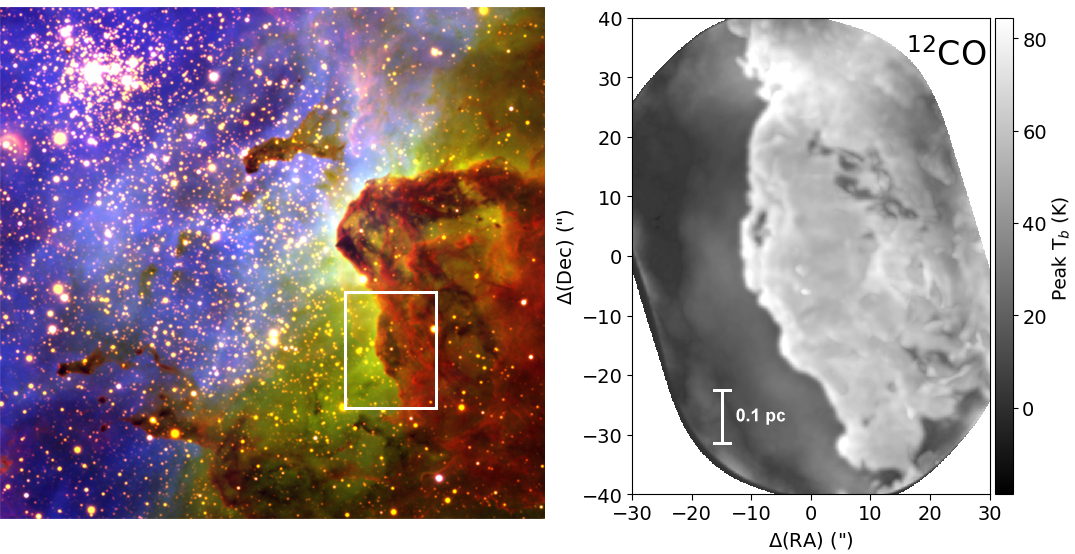
Figure 1: Left: Composite RGB image of the Western Wall region in the Carina nebula from Hartigan et al. (2015). The image spans approximately 4.25 pc in RA and 4.0 pc in DEC. Red, green, and blue colors indicate emission from H₂, Br$\gamma$, and [O III], respectively. The stellar cluster at the top-left is Trumpler 14. The white rectangle outlines the region expanded at right. Right: Peak brightness temperature in degrees K in the velocity interval $-$28.5 km s^-1 to $-$19.0 km s^-1 in ¹²CO J = 2 - 1 recorded by ALMA toward the Western Wall. The angular resolution of the ALMA observations (FWHM of the synthesized beam) is 1.0″ for ¹²CO J = 2 - 1. The spatial coordinates $\Delta$RA and $\Delta$DEC are relative to the central map position of $\alpha$(2000) = 10:43:30.64, $\delta$(2000) = $-$59:35:57.4.

The observations utilized the 12-m, 7-m, and total power antennas. For Band 6, the 12-m array achieved maximum baselines of 390 m, 460 m, and 6.3 km in three separate epochs, and the 7-m data derives from a compact configuration with maximum baselines of about 45 m. This combination of 12-m, 7-m, and total power data probes emission on spatial scales as small as about 0.04″ at 1.3 mm. We acquired Band 8 data in a single epoch when the 12-m array was on an extended configuration with baselines up to 6.3 km, resulting in a theoretical maximum angular resolution of 0.02″. Small mosaics of 5 and 13 pointings for the 7-m and 12-m arrays at Band 6, and 22 and 57 pointings for the 7-m and 12-m arrays at Band 8 sufficed to cover the region of interest. In all cases, mosaic pointings were spaced by 0.511$\times$HPBW (Half Primary Beam Width) to sample the emission at the Nyquist spatial frequency. We calibrated the data using version 4.7.0 of the ALMA pipeline except for the Band 8 data from the 12-m array, which we acquired as a non-standard mode and calibrated manually using CASA 4.7.2. Table 3 in the Appendix lists the calibrators we used to derive complex phase and amplitude gains, and also presents the observing log of the entire data set.

We combined the single-dish and interferometric observations for the line emission in the Fourier space using a modified version of TP2VIS (Koda et al., 2019) as described in the Appendix. Images of the continuum emission used only 7-m and 12-m array interferometric data. The task TCLEAN (CASA Version 5.6.0) generated both the continuum and line images. We performed image deconvolution in Band 6 using multi-scale cleaning with Briggs weighting and a robust parameter equal 1. This procedure resulted in a synthesized beam size of 0.7″ in the continuum and 1″ in the CO lines. For band 8, the continuum reductions adopted a Briggs weighting with robust 0.3 and applied a uv-taper corresponding to an on-sky FWHM of 0.25″. UV-tapering the band 8 data is necessary to remove the longest baselines and to achieve a synthesized beam with low side lobes. The angular resolution of the final Band 8 images is 1.2″$\times$0.9″ in the line emission and 1.1″$\times$1.4″ in the continuum.

3 Emission Line and Continuum Maps of ¹²CO, ¹³CO, C¹⁸O and [C I]

In this section we present results of the emission-line and continuum maps of the area outlined in Fig. 1. Sec. 3.1 identifies individual clouds superposed along the line of sight from their radial velocities and considers several compact sources visible in the ¹²CO datacube. Sec. 3.2 calculates [C I] and CO optical depths and abundance ratios, compares the [C I] data with CO, estimates a mass for the Western Wall cloud, examines spatial offsets between the emitting layers of the PDR, and provides an overview of the kinematics within the Western Wall cloud. Sec. 3.3 considers what the continuum observations of the region reveal about grain size, and investigates how the PDR influences the morphology of the densest concentration of clumps and cores in the area.

3.1 Overview of the Clouds and Compact Sources in the Map

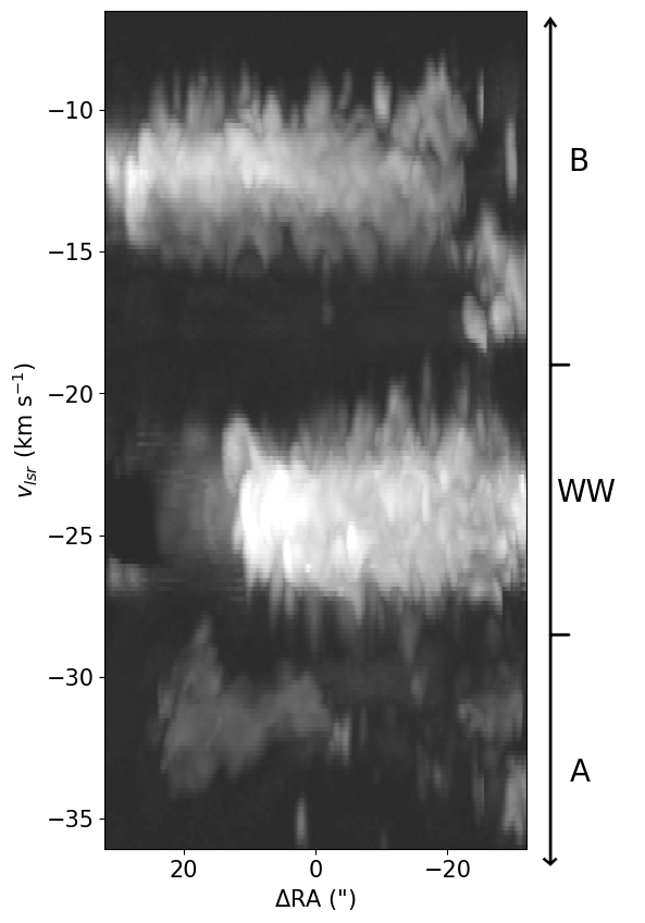
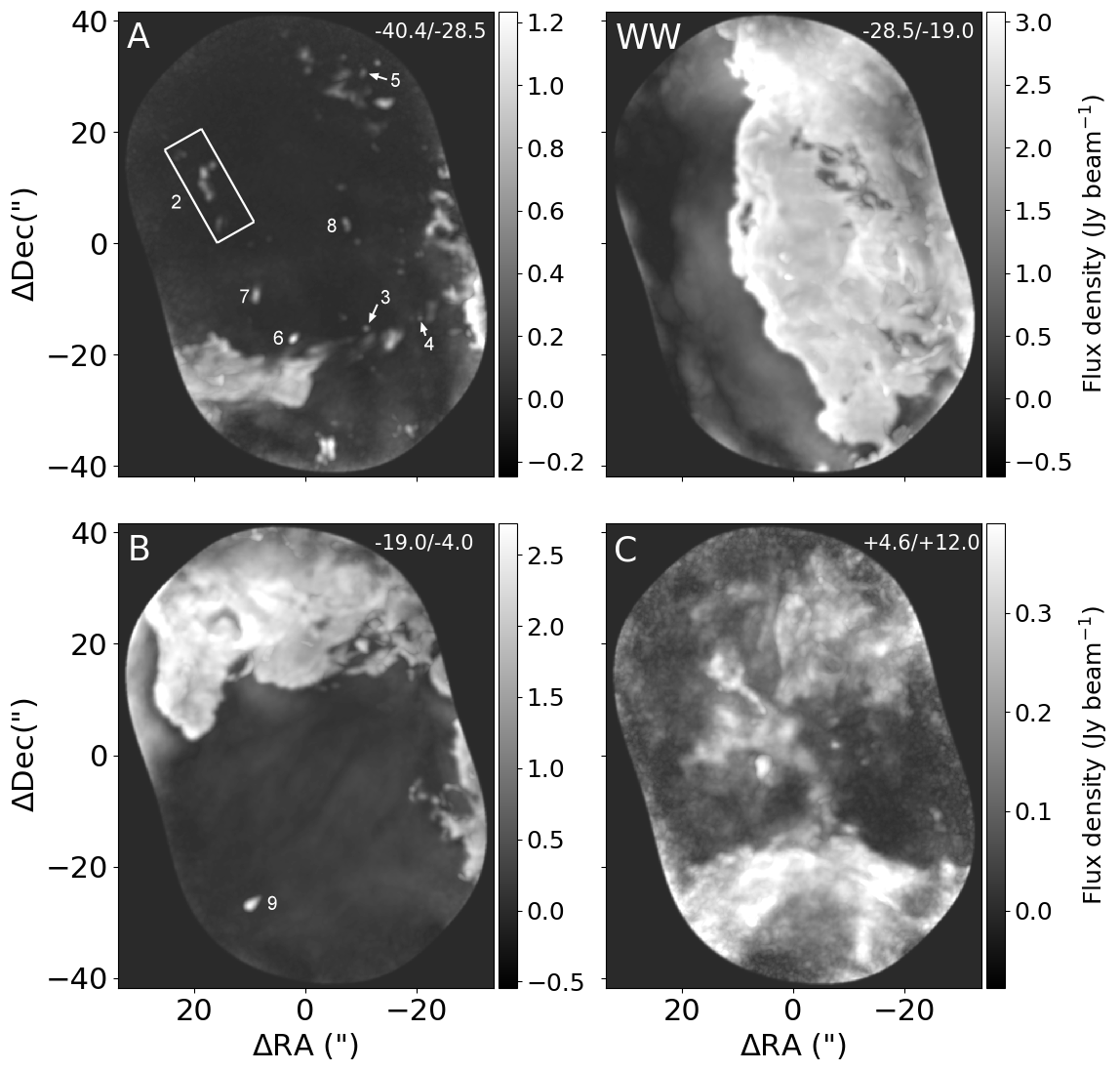
Figure 2: Left: position-velocity diagram of ¹²CO recorded in the area shown in Fig. 1, integrated over all declinations in the map. Right: maps of the peak intensity in the velocity range indicated in the top right of each panel. The ¹²CO emission separates into four distinct ranges in velocity. Velocity range A includes emission from $-$40.5 km s^-1 to $-$28.5 km s^-1, and contains several compact sources labeled with numbers as well as two clouds that appear unrelated to the Western Wall. The Western Wall cloud emits from $-$28.5 km s^-1 to $-$19.0 km s^-1 in CO, with most of the emission in the range from $-$21.3 km s^-1 to $-$27.1 km s^-1, and extends from north to south across the field of view. Region B, spanning $-$19.0 km s^-1 to $-$4 km s^-1, shows molecular clouds that reside within Carina OB1 but are unrelated to the photodissociation front. Clouds with velocities between +4.6 and +12.0 km s^-1 (region C), are diffuse and cover the entire field. The spatial offsets are defined relative to the central map position in Fig. 1.

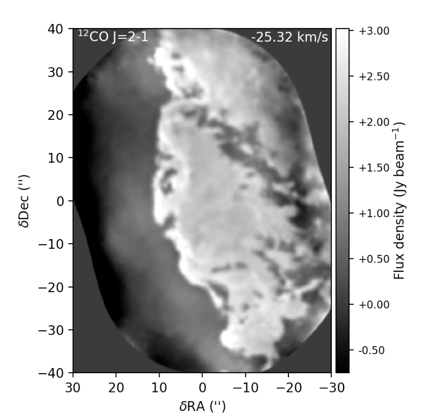
Figure 3: Animation through the channels in the ALMA ¹²CO datacube. The image is centered at $\alpha$(2000) = 10h43m30.64s, $\delta$(2000) = $-$59°35′57.4″, and ranges from $-$45.16 km s^-1 to $+$5.16 km s^-1 V_lsr in increments of 0.166 km s^-1. Each frame is normalized to the value indicated by the scale bar at right. The video duration is 75 seconds.

Fig. 1 shows that the region mapped by our ALMA observations covers roughly the southern half of the Western Wall, easily visible in the optical/infrared composite as a bright irradiated cloud characterized by H₂ fluorescence at the PDR interface and Br$\gamma$ emission that arises in the photoevaporative flow (Hartigan et al., 2015, 2020). A compact cluster of young stars known as Trumpler 14 situated about 3.5′ to the northeast of the Western Wall is the main source of irradiation, though additional massive stars, including $\eta$ Car and others in the young cluster Trumpler 16 located off the frame to the southeast, also irradiate the cloud.

The position-velocity diagram of ¹²CO emission shown in Fig. 2 and in the animation in Fig. 3 uncovered several distinct molecular clouds that lie within the area mapped by our observations. We refer to these features as ‘clouds’ rather than ‘clumps’ because their radial velocities differ markedly and they are unlikely to be associated with one-another. We use the term ‘clump’ to refer to small structures within our datacubes (see section 4). Carina is located within a degree of the galactic plane, so it would not be unusual to observe multiple molecular clouds projected along the line of sight.

Beginning with the most negative velocities in the data cube (panel A in Fig. 2), the first extended emission from molecular clouds in the region appears around $-$35 km s^-1 at the far southwestern edge of the mapped region near ($\Delta$RA,$\Delta$Dec) = ($-$25^′′,$-$15^′′). Because this feature only occurs at the edge of our map and is superposed spatially upon the molecular cloud that defines the Western Wall, it is difficult to identify any counterpart in the optical/IR composite with certainty. A second coherent structure in Panel A spans $\sim$ $\Delta$RA = 0^′′ to +15^′′, $\Delta$DEC = $-$30^′′ to $-$20^′′ and velocity range $-$29 km s^-1 to $-$34 km s^-1. This feature may be associated with a small area of dust that appears to lie in front of the H II region in Fig. 1. In any event, neither of these objects seems to be associated with the irradiated wall.

The dark cloud that makes up the irradiated Western Wall ranges in velocity between about $-$19 km s^-1 and $-$28.5 km s^-1. At the edges of its velocity range, the Western Wall molecular cloud breaks into fragments, probably because only the densest portions are optically thick at those velocities. The Western Wall becomes relatively smooth around $-$24 km s^-1 where the entire wall is optically thick. Overall, the shape of the Western Wall traced in CO follows the shape of the irradiated interface defined by the fluoresced H₂ emission. We discuss the velocity field within the Western Wall more fully in the next section.

The molecular cloud visible in panel B of Fig. 2 ($-$19 km s^-1 to $-$4 km s^-1) along the northern edge of the map (hereafter ‘Cloud B’) is associated with the Carina complex, as the edge of the cloud appears weakly in the H₂ and Br$\gamma$ images. However, this cloud is located behind the Western Wall, based on the extra Br$\gamma$ emission in this area as compared to what occurs at the position of the Western Wall molecular cloud, and the fact that the Western Wall blocks out what we can see of Cloud B in Fig 1. Cloud B provides a good comparison for the Western Wall cloud, in that both are located in the Carina complex but the two clouds have markedly differing radiation environments. In this velocity range there is also a strip of CO emission that runs vertically along the far western edge of the map and corresponds to the edge of a feature that also appears weakly in archival Spitzer images of the region (Tapia et al., 2015; Brooks et al., 2003). This emission arises from another, probably foreground molecular cloud in this area.

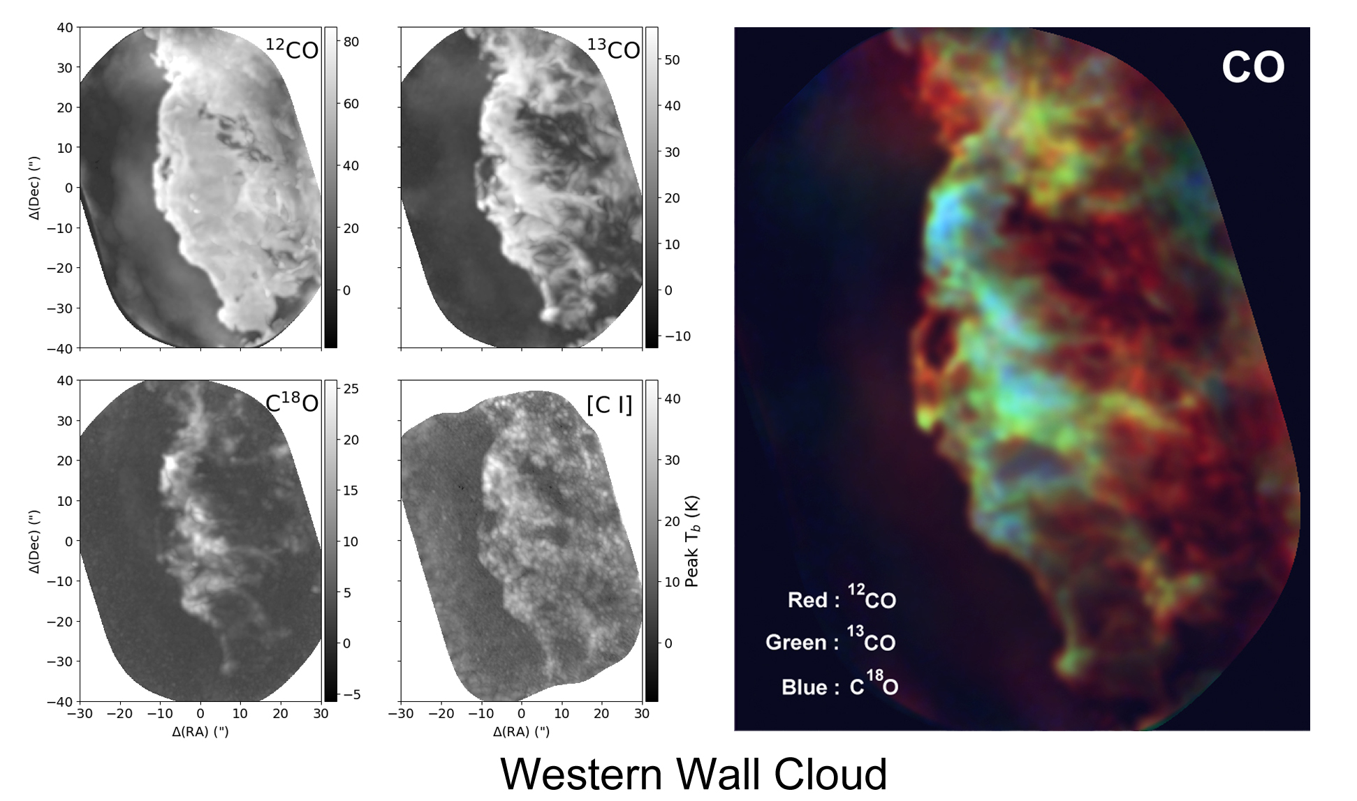
Figure 4: Left: Maps of the peak intensity of the ¹²CO, ¹³CO, C¹⁸O, and [C I] lines expressed in units of the brightness temperature (K). Right: Color composite of the CO emission from the Western Wall molecular cloud, constructed by integrating the datacubes of ¹²CO (red), ¹³CO (green), and C¹⁸O (blue) between V_lsr velocities $-$21.28 km s^-1 and $-$27.09 km s^-1. The densest portions of the cloud (areas with the strongest C¹⁸O emission) occur closer to the PDR interface relative to the ¹²CO image, which is optically thick everwhere.

At velocities more positive than those of the clouds in panel B of Fig. 2, the data cube is empty for a span of nearly 10 km s^-1 until an array of molecular clouds begins to fill the field (panel C). These clouds have no counterparts in the optical/IR composite, and are most likely to be background objects.

Table 1: Compact Sources in the ¹²CO Datacube

Source	$\alpha$ (2000)	$\delta$ (2000)	VLSR (km s-1)	IR Counterpart	Notes
(1)	(2)	(3)	(4)	(5)	(6)
1	10:43:28.84	$-$59:36:12.0	$-$42.0	H2 nebula
2	10:43:33.09	$-$59:35:44.4	$-$37 to $-40$	none	An arc with multiple knots; N-S velocity gradient
3	10:43:29.22	$-$59:36:12.6	$-$39.1	dark globule
4	10:43:27.94	$-$59:36:10.8	$-$38.4	dark globule
5	10:43:29.29	$-$59:35:26.5	$-$36.4	none
6	10:43:30.93	$-$59:36:14.3	$-$36.2	dark globule	Bipolar, PA $\sim$ 315 degrees
7	10:43:31.85	$-$59:36:06.7	$-$31.9	none
8	10:43:29.69	$-$59:35:53.7	$-$31.6	none	Bipolar, PA $\sim$ 20 degrees
9	10:43:32.00	$-$59:36:24.5	$-$5.4	proplyd	Teardrop-shaped extension at PA $\sim$ 305 degrees

The ¹²CO datacubes contain a dozen or so compact sources whose emission is restricted to an interval of $\sim$ 1 km s^-1, and are clearly distinct from the velocity fields associated with the spatially extended molecular clouds (see Table 1). These sources are labeled with numbers in Fig. 2 with the exception of object 1, which is too blueshifted to be included in the figure. Most of these sources appear to be individual globules situated either foreground or background to the Western Wall cloud, but some may represent outflows. Objects 3, 4, and 6 appear as small, bright-rimmed dark globules about 0.5 arcseconds (1150 AU) in diameter superposed upon the Western Wall cloud in H₂ and Br-$\gamma$ adaptive optics images of the region (Hartigan et al., 2020), while object 1 lies near a small arc of H₂ emission that may or may not be related to the CO source. Objects 6 and 8 have bipolar spatial morphologies in the ¹²CO cubes, and exhibit velocity gradients suggestive of an outflow. Object 2 has several knots arrayed along an arc with a clear velocity gradient, while object 9 is a teardrop-shaped cloud that resembles a proplyd, and glows faintly in H₂ but is invisible at Br-$\gamma$. This latter object, situated to the east of the Western Wall cloud, is the only source in Table 1 with a more redshifted radial velocity than the Western Wall cloud. The tail of the proplyd is more redshifted than the head, and breaks into three knots in its most redshifted velocity slice. Object 9 is probably located behind the Western Wall cloud, as this source has similar radial velocities to Cloud B (Fig 2), which must be a background object as noted above. Some of the knot-like morphology we observe in Fig 2 on scales of the beam size (e.g. the string of knots that comprise object 2) may be enhanced by noise or from uncertainties in the reconstruction of the images from the raw ALMA data. We defer additional discussion of these objects to future works.

3.2 The Western Wall Molecular Cloud

3.2.1 Optical Depths, Depletion from Irradiation, and Cloud Mass

Maps of the ¹²CO, ¹³CO, C¹⁸O, and [C I] line peak intensity recorded in the Western Wall velocity range are shown in Fig. 4. The intensity in the maps above the microwave background is in units of the brightness temperature $T_{b}$, calculated using the Planck equation as

$$T_{b}=\frac{h\nu}{k}\left[\ln\left(\frac{2h\nu^{3}\Omega}{c^{2}F_{\nu}}+1\right)\right]^{-1}.$$ (1)

where $F_{\nu}$ is the specific flux integrated over a resolution element defined by the solid angle $\Omega$ = $\pi\theta_{min}\theta_{max}$ / $(4\ln 2)$, where $\theta_{min}$ and $\theta_{max}$ are the minimum and maximum FWHM of the synthesized beam. The ¹²CO emission reaches a peak brightness temperature between 80 K and 90 K along the photoevaporation front where the stellar radiation heats the molecular cloud.

The observed brightness temperatures are somewhat lower than those found in the Orion Bar ($\sim$ 150 K) and NGC 7023 ($\sim$ 110 K), where the PDRs are located closer to their respective photoionization sources (Joblin et al., 2018). For example, the distance between $\theta^{1}$ Ori C, the hottest star in the Trapezium, and the main ionization front is about 0.25 pc, whereas the Western Wall is about 2.3 pc in projected distance away from Tr 14. Brooks et al. (2003) lists the irradiation flux at the Orion Bar as $\sim$ $4\times 10^{4}$ $G_{0}$ (where $G_{0}=1$ corresponds to a flux of $1.6\times 10^{-3}$ erg cm^-2 s^-1), while recent models of the Western Wall give a comparable value of $3\times 10^{4}$ $G_{0}$ (Wu et al., 2018). However, it is important to keep in mind that the Western Wall has $\sim$ 50 - 100 times the area of the Orion Bar, so radiation can influence molecular clouds in Carina on much larger scales than it can in less-massive regions such as Orion.

We can get some idea as to the optical depths we might expect for a line by calculating the optical depth at line center for thermal broadening under typical molecular cloud conditions and assuming standard abundances (see Eqn. C11 in the Appendix):

$$\tau_{0}=1741\ \lambda^{3}A_{21}\frac{g_{2}}{g_{1}}m^{0.5}T^{-0.5}S\frac{{\rm N}_{1}}{{\rm N}_{{\rm TOT}}}\frac{{\rm N}_{{\rm TOT}}}{{\rm N}_{H}}\frac{{\rm N}_{\rm H}}{10^{21}{\rm cm}^{-2}}$$ (2)

where $\lambda$ is the wavelength in microns, A₂₁ is the Einstein-A value for the transition in s^-1, g₂/g₁ is the ratio of the statistical weights between the upper and lower states, m is the species mass in amu, T is the temperature in K, S is a factor that corrects for stimulated emission and for departures from LTE, and the final three terms are, respectively, the fraction of species in the lower level state, the abundance of the species respective to hydrogen, and the hydrogen column density.

Taking T $\sim$ 30 K, an abundance ratio C I/CO $\sim$ 0.2 in the PDR with 40% of C locked in grains (see Appendix C, Table 4, and discussion below), and a fiducial hydrogen column density of 2.7$\times$10²¹ cm^-2, which corresponds to a visual extinction A_V $\sim$ 1 for a normal reddening law (Liszt, 2014), we find C¹⁸O is optically thin with $\tau$ $\sim$ 0.2 (with no radiative depletion), and [C I] should have an optical depth $\sim$ 0.8. ¹³CO should be more optically thick with $\tau$ $\sim$ 1.3, and ¹²CO has a very high optical depth of $\tau$ $\gtrsim$ 100. These numbers are meant only as guides to help interpret the images, as following the layered distribution of molecules, atoms, ions, and dust within a PDR is a complex problem that requires sophisticated modeling (e.g. Spaans, 1996). Nonetheless, overall we expect ¹²CO to be very optically thick and to probe only the outer layer of the cloud, ¹³CO to be either optically thick or thin depending on the region, [C I] to be mostly optically thin except perhaps in the dense cores, and C¹⁸O to be optically thin everywhere. These expectations are in agreement with the results in Fig. 5 described in Sec. 3.2.1. Optically thin lines tracers such as C¹⁸O J = 2 - 1, and, to a lesser extent [C I] 609 $\mu$m, probe the densest portions of the clouds. Of the two tracers, C¹⁸O has the better signal-to-noise, as its J = 2 - 1 1.3 mm line emits in ALMA’s Band 6, in contrast with the more difficult observation of [C I] 609$\mu$m in ALMA’s Band 8.

The line optical depth $\tau_{\nu}$ for a slab of gas in LTE at temperature T depends upon the observed specific line intensity I_ν via

$${\rm I}_{\nu}={\rm B}_{\nu}({\rm T})(1-e^{-\tau_{\nu}}),$$ (3)

where B_ν is the Planck function. With assumptions of constant temperature and fixed abundance ratios between ¹²CO, ¹³CO and C¹⁸O, the observed line ratios between these isotopologues in principle provide an optical depth map for the region at each velocity.

Unfortunately, this simple procedure fails for two reasons. First, the inner regions of molecular clouds are more shielded from external radiation, and thus are colder than the outer layers of the cloud. Because $\tau$ $\sim$ 1 occurs closer to the surface of a cloud for ¹²CO than it does for a less abundant isotopologue such as ¹³CO, the intensity of ¹²CO can be significantly higher than that of ¹³CO even when both lines are optically thick. Fig. 4 illustrates this effect, where the peak brightness temperature in ¹²CO is about 80 K, while that in ¹³CO is $\sim$ 50 K.

An even larger error is introduced by assuming constant abundance ratios for ¹²CO : ¹³CO : C¹⁸O throughout the cloud. As described by Miotello et al. (2014), the abundance ratio of, for example, C¹⁸O / ¹²CO can be depleted by up to a factor of 20 within irradiated clouds owing to processes that lead to selective dissociation of the different CO isotopologues. Photodissociation of CO is dominated by absorption into discrete bands above the CO dissociation energy of $\sim$ 11.1 eV and below the H-ionization limit of 13.6 eV (e.g. Letzelter et al., 1987), and the energy levels of these bands differ enough between C¹⁸O and ¹²CO, that ¹²CO effectively self-shields against dissociation close to the surface of the cloud without also shielding C¹⁸O. As a result, C¹⁸O is dissociated much deeper into the cloud (Bally & Langer, 1982; Visser et al., 2009).

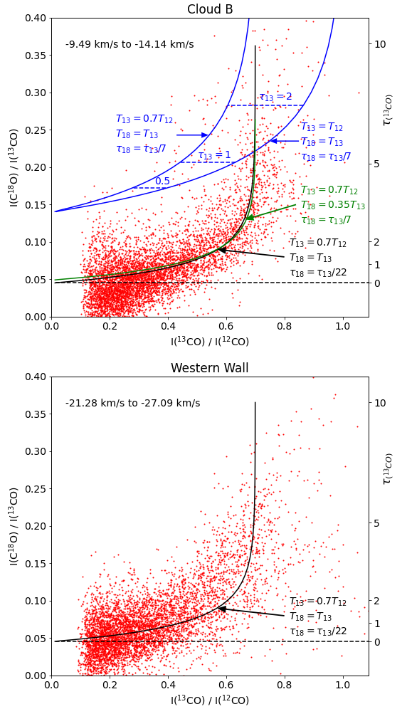
Figure 5: Observed intensity ratios between ¹²CO, ¹³CO, and C¹⁸O for Cloud B (top) and the Western Wall cloud (bottom). Ratios were taken from positions separated by $\sim$ 1 beam size within each 0.166 km s^-1 velocity channel spanned by the cloud, and are shown for all points in the datacube where the ¹³CO intensity exceeds 0.25 Jky/beam. Optical depths in ¹³CO for the black curve are shown on the scale at right. The simple models shown are discussed in the text.

Fig. 5 displays the observed line ratios between the three isotopologues of CO for the velocity range and spatial extent of Cloud B, located along the northern boundary of our map (Fig. 2) and for the Western Wall cloud. Cloud B is defined by a 40″ $\times$ 30″ box centered at $\alpha$(2000) = 10:43:31.9, $\delta$(2000) = $-$59:35:40.4 and encompassing $-$9.49 km s^-1 to $-$14.14 km s^-1, and the Western Wall cloud by a 36″ $\times$ 72″ box centered at $\alpha$(2000) = 10:43:30.0, $\delta$(2000) = $-$59:35:55 between $-$21.28 km s^-1 and $-$27.09 km s^-1. Cloud B is in the Carina Nebula, as it appears weakly in H₂ (Fig 1). However, its relative faintness in H₂ and lower peak temperature in ¹²CO ($\sim$ 60 K instead of $\sim$ 80 K for the Western Wall cloud) implies that the radiation field impinging upon Cloud B is substantially lower than it is for the Western Wall. Hence, any differences in the emission line ratios between these two clouds informs how radiation affects the isotopologues of CO in molecular clouds.

The blue curves in the diagrams illustrate the expected line ratios for the simplest case of fixed cosmic abundances and temperatures, where N(¹³CO) / N(C¹⁸O) = 7 and N(¹²CO) / N(¹³CO) = 77 (Wilson & Rood, 1994). The model with equal temperatures for ¹²CO and ¹³CO does not agree with the observations. Adopting T_b(¹³CO) = 0.7T_b(¹²CO) to account for the warmer temperatures associated with the ¹²CO emission near the surface of the cloud reproduces the asymptotic behavior of the I(¹²CO) / I(¹³CO) ratio where the regions are brightest and most optically thick, but this model fails to account for the anomalously low I(C¹⁸O) / I(¹³CO) ratio present in both clouds.

The black curve is a model calculated by reducing the abundance of N(C¹⁸O) / N(¹³CO) from 1/7 to 1/22, and this model matches the data reasonably well for Cloud B albeit with significant scatter. Adopting a greatly reduced temperature in the C¹⁸O emitting region relative to the temperature in the ¹³CO region (green curve) agrees equally well with the data, however this model would imply T(C¹⁸O) $\sim$ 0.25 T(¹²CO) $\lesssim$ 20 K, which seems rather low. The scatter at the left side of the plot arises primarily from low flux values, especially in the C¹⁸O map, while the scatter in the upper right probably arises mostly from variations in the temperature ratio between ¹²CO and ¹³CO across the region.

Although the irradiated Western Wall cloud generally follows the same trends as we see in Cloud B, the overall fit of the model to the data is not as good, most noticably where the data congregate above the black curve as the curve begins to bend upward. The differences between the model and Western Wall data are in the sense that C¹⁸O appears more abundant or warmer in the data relative to the model when $\tau$(¹³CO) $\sim$ 2. Regardless of the cause, there is a systematic difference between the isotopologue CO ratios in the highly-irradiated Western Wall cloud, and the more weakly-irradiated Cloud B.

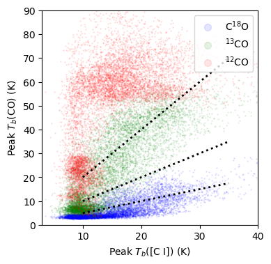
Figure 6: Peak brightness temperatures of the J = 2 - 1 transitions of ¹²CO (red), ¹³CO (green), and C¹⁸O (blue) plotted against the peak brightness temperature of [C I] 609 $\mu$m within the Western Wall molecular cloud. The dashed lines are fiducials with slopes of 0.5, 1, and 2. There is a nearly linear relationship between the peak brightness temperatures of the [C I] and C¹⁸O lines.

The axes on the right side of the plots in Fig. 5 show that ¹³CO ranges in optical depth within each velocity channel from optically thin to a maximum of $\sim$ 10. Hence, C¹⁸O is optically thin throughout the region, with an optical depth $\tau_{18}$ $\lesssim$ 0.5, and we can integrate the observed line flux to estimate a mass for the Western Wall cloud. The total flux of the line integrated over the Western Wall cloud between $-$27.09 km s^-1 and $-$21.28 km s^-1 is $1.7\times 10^{-15}$ erg cm^-2s^-1 with an error of 10% dominated by the systematic errors associated with the absolute flux calibrations in the total power data. At a distance of 2.3 kpc this flux translates to a line luminosity of L₂₁ = $1.1\times 10^{30}$erg s^-1. The line luminosity relates to the total number of C¹⁸O molecules in the J = 2 level N₂(C¹⁸O) via

$${\rm N}_{2}({\rm C}^{18}{\rm O})=\frac{{\rm L}_{21}}{{\rm A}_{21}{\rm h}\nu}=1.26\times 10^{51},$$ (4)

where we have used A₂₁ = $6.01\times 10^{-7}$ s^-1 as the Einstein-A coefficient and h$\nu$ = $1.45\times 10^{-15}$ erg as the transition energy.

For a characteristic temperature of 30 K and LTE population, 25% of the C¹⁸O molecules are in level 2, so adopting a conversion factor of 22$\times$77 = 1694 between the abundances of C¹⁸O and ¹²CO implies $8.5\times 10^{54}$ ¹²CO molecules. The abundance ratio between of H₂ and gaseous CO in star-forming regions varies between $\sim$ 3100 and 14500 (Lacy et al., 1994, 2017). Adopting 6000 for this value we calculate the mass of the portion of the Western Wall cloud in our ALMA datacube to be 85 M_⊙. The same calculation done with ¹³CO assuming a ratio of ¹²CO/¹³CO = 77 gives 52 M_⊙ for the mass, a lower value as expected given that much of the ¹³CO is optically thick.

Based on their lower-resolution ¹²CO and ¹³CO maps in the velocity range between $-$25 km s^-1 and $-$22 km s^-1, Brooks et al. (2003) found a much higher mass of $\sim$ 500 M_⊙ assuming either virial equilibrium or using a conversion from ¹³CO to H₂ applicable if the ¹³CO is optically thin. However, these estimates cover an area five times that of our map, and virial calculations will overestimate the masses in this region owing to the multiple velocity components along the line of sight. Fig. 1 also suggests that the entire Western Wall cloud contains several dense regions that are not included in our ALMA data. Overall, the Western Wall cloud is larger in area by a factor of $\sim$ 2 - 3 than our mapped region, so our best estimate for the total mass of the entire cloud is $\sim$ 240 M_⊙, though this number could change by a factor of two with more extensive mapping of the region. The uncertainties in these mass estimates are dominated by systematic errors associated with the H₂/CO conversion factors and the abundance ratios of the isotopes of CO, and are likely to be a factor of two given the observed range of these values between different molecular clouds.

3.2.2 [C I] in the Western Wall Cloud

In the Orion A and Orion B PDRs, there is a correlation between the brightness temperature of the [C I] ³P${}_{1}-^{3}$P₀ and that of ¹³CO J = 1 - 0 line, with $T_{b}(\textrm{[C~{}I]})\sim 0.6\times T_{b}(\textrm{${}^{13}$CO})$ (Ikeda et al., 1999, 2002). The intensity ratio indicates that [C I] 609$\mu$m has an optical depth that varies between about 0.3 and 2 and implies C I column densities between $10^{17}$ and 10¹⁸ cm^-2. These studies found that the abundance ratio between atomic carbon and CO molecules is almost constant between 0.1 and 0.2 across regions with different levels of star formation activities, such as Orion KL and the much more quiescent L1641 dark cloud. Hence, the C I/CO ratio is insensitive to the level of UV radiation, at least in Orion.

The ratio between the intensities of the CO and the C I lines measured toward the Western Wall region is shown in Fig. 6. Unlike Ikeda et al. (2002), our observations targeted the J = 2 - 1 transition of CO, covered three CO isotopologues, and resolved emission on spatial scales almost 30 times smaller than those observed in Orion. Despite the observational differences, we find a similar correlation between [C I] and CO line intensities. As expected for optically thin lines with an approximately constant abundance ratio, the correlation between [C I] and C¹⁸O is nearly linear, with the brightness temperature of [C I] 609 $\mu$m about twice that of C¹⁸O J = 2 - 1. However, there is scatter in the relationship and there are features that are unique to the [C I] map. For example, in Fig. 4 the [C I] emission lacks the bright, diffuse features present in the center of the C¹⁸O map. [C I] also shows additional small droplet-shaped overdensities with clear velocity gradients that are less apparent in C¹⁸O, and are approximately the same size of the beam ($\sim 1\arcsec$).

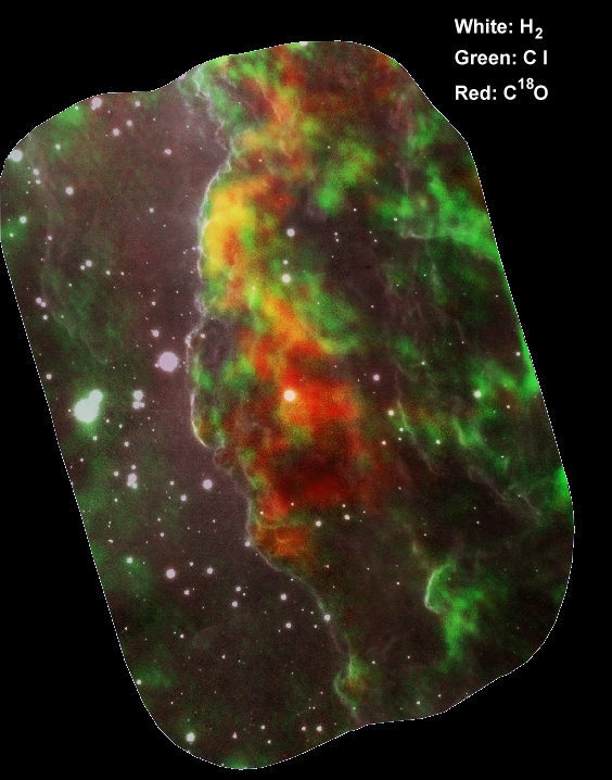
Figure 7: Color composite of H₂, [C I], and C¹⁸O in the Western Wall molecular cloud. The H₂ image in white is from Gemini South’s adaptive optics imager (Hartigan et al., 2020), and shows fluorescence at the boundary of the cloud. The [C I] (green), and C¹⁸O (red) images extracted from the ALMA datacubes between V_lsr velocities $-$21.28 km s^-1 and $-$27.09 km s^-1 are mostly optically thin. There is a general progression from H₂ to [C I] to C¹⁸O as one moves deeper into the cloud from left to right.

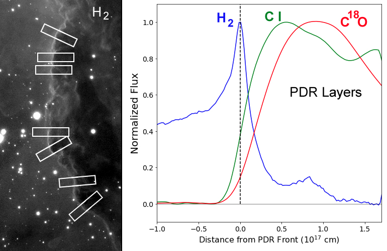
Figure 8: Average spatial offsets between H₂, C I, and C¹⁸O emission in the Western Wall molecular cloud. The average spatial line profiles shown in the graph at right were extracted from the seven boxed areas marked in the H₂ image from Hartigan et al. (2020) at left. The H₂ image includes continuum, which produces the plateau of emission upstream (to the left) of the PDR. The C I and C¹⁸O profiles were restricted to the velocity range associated with the cloud.

While there is a positive correlation between [C I] 609 $\mu$m and both ¹³CO J = 2 - 1 and ¹²CO J = 2 - 1 in Fig. 6, the relations do not fall on a line, especially for ¹²CO, which is very optically thick so its brightness temperature saturates at the thermal temperature of the gas. As in Orion, the peak brightness temperature of [C I] 609 $\mu$m is about half of that of the ¹³CO J = 2 - 1 over most of the Western Wall cloud.

3.2.3 Observable PDR Layers

Our ALMA data are ideal for illustrating the overall layered structure of a PDR because we observe both [C I] and C¹⁸O, and the C¹⁸O is optically thin and the [C I] mostly so. [C I] is predicted to have an emitting layer that lies closer to the PDR front than CO does (Spaans, 1996). Moreover, the Western Wall has a convex shape and we view it in profile, which greatly reduces problematic projection effects that complicate images of concave cavities such as the Orion Bar. Fig. 7 overlays the latest high-resolution adaptive-optics image of the region in H₂ (Hartigan et al., 2020) with the [C I] and C¹⁸O maps. As predicted by theory, H₂ traces the interface where radiation impinges upon the cloud. The interface is followed by a complex flocculent morphology in the ALMA images, but there is order in the sense that all the bright C¹⁸O features have a layer of [C I] between the CO and the H₂.

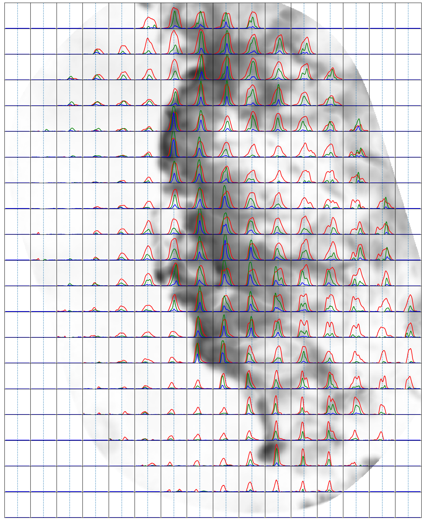
Figure 9: Spectra of the ¹²CO (red), ¹³CO (green), and C¹⁸O (blue) J = 2 - 1 lines recorded toward the Carina Western Wall molecular cloud. For a better comparison, the intensity of the ¹³CO and C¹⁸O lines were multiplied by a factor of 2 and 5, respectively. The spectra were obtained by spatially integrated the observed line emission across square regions of 4″$\times$4″, and span velocities between -29.59 km s^-1 to $-19.62$ km s^-1, from left to right in each box. As a reference, vertical dotted lines indicate the average velocity, -24.60 km s^-1 of the cloud. The background image shows the peak intensity map of ¹³CO. The wider and multi-peaked spectra in the cloud’s interior are likely due to multiple clumps overlapping along the line of sight. Conversely, the clumps located along the Western Wall’s edge have spectra with a single peak.

The offsets are perhaps easiest to see in Fig. 8, which combines the spatial emission profiles along seven transects, each 2″ in width, chosen to contain bright emission and to avoid stars. The excellent spatial resolution of the H₂ adaptive-optics image helps greatly to reduce stellar contamination in these profiles, but continuum light adds to the integrated flux in the H₂ profiles, especially east of the PDR in the direction of the radiation sources. Nonetheless, the integrated profiles display a sharp H₂ peak, which we take to define the location of the PDR. The profiles in Fig. 8 exhibit the expected layered structure, with offsets between the H₂, C I, and C¹⁸O emitting layers of $\sim$ $10^{17}$ cm, similar to the offsets observed between H₂ and Br-$\gamma$ in this region by Carlsten & Hartigan (2018).

3.2.4 Kinematics

Figure 9 depicts the complex kinematics within the Western Wall molecular cloud in the lines of ¹²CO, ¹³CO and C¹⁸O. Regions close to eastern edge where the Western Wall is irradiated have relatively narrow, single-peaked lines, whereas regions away from the photo-evaporation front exhibit wider, and sometimes multiple-peaked profiles. These multiple peaks make sense from a geometrical standpoint, as our line of sight passes through more of the cloud to the west as the projected distances from the front increase, so more clumps will appear within the beam if the clumps are distributed through the cloud. The line kinematics uncovered a large-scale velocity gradient south-to-north across the Western Wall cloud, with line emission from the north part of the object peaking at a velocity of about $-$24 km s^-1 and the south part peaking at velocities of $-$26 km s^-1. This gradient is particularly striking in the animation (Fig. 3). We defer further analysis of the kinematics within the Western Wall cloud and its connection to turbulence to a companion paper (Downes et al., 2022).

3.3 Comparing CO and Continuum Maps, Distortion of Cores at the PDR, Dust Properties

Eqn. 3 provides an optical depth measurement at each position and velocity from the observed intensity ratio between ¹³CO and C¹⁸O, under the assumption that the two species emit at the same temperature. Because all areas with substantial C¹⁸O flux are optically thick in ¹³CO (Fig. 5), this measurement is independent of the relative abundances of ¹³CO and C¹⁸O. The left panel of Fig. 10 shows the maximum optical depth achieved across the datacube for the Western Wall cloud. Interestingly, regions with higher optical depth are aligned along the Western Wall, suggesting that the photoevaporation front is responsible for compressing the molecular gas along this interface. In particular, the brightest knots within the boxed area tend to curve in the same direction as the PDR interface does. However, the flattened structures in C¹⁸O do not resolve into separate pillars, as should occur when a radiation front wraps around dense knots.

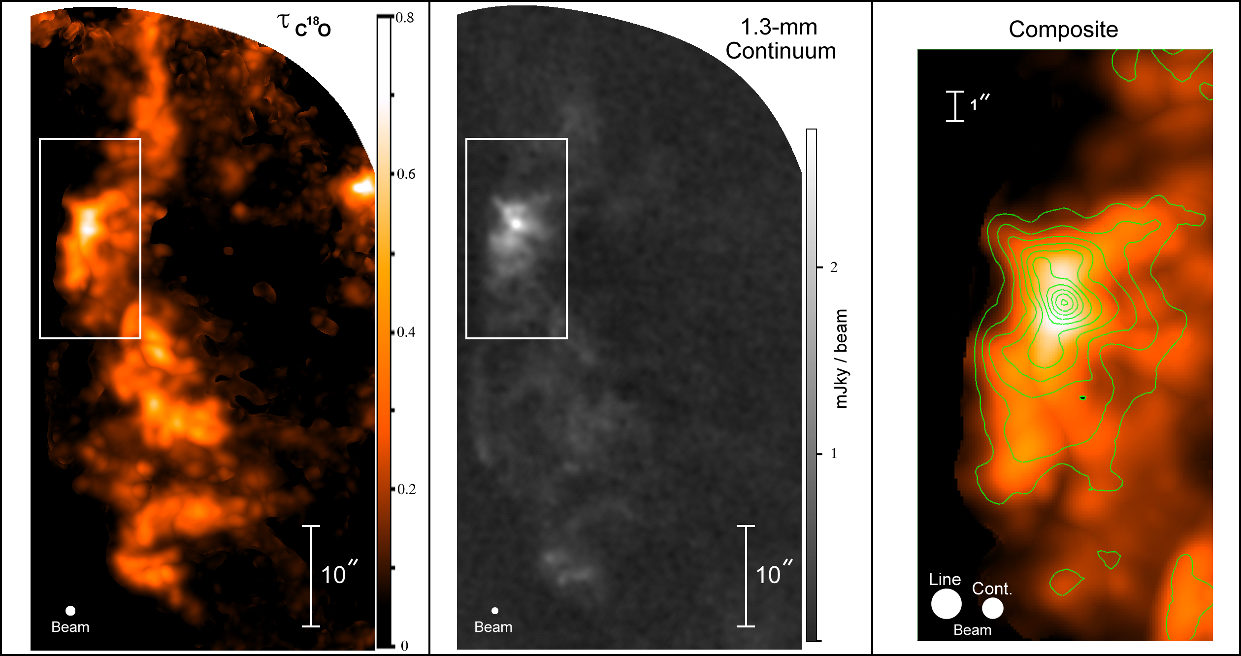
Figure 10: Left: Map of the peak optical depth in C¹⁸O for the Western Wall Cloud. The boxed region centered at $\alpha$ (2000) = 10:43:31.6 $\delta$ (2000) = $-$59:35:40.0 subtends 10″ $\times$ 20″, and contains several bright resolved structures. Center: 1.3 mm continuum map, acquired with a circular 0.7″ beam. There is a bright unresolved core near the location of peak C¹⁸O optical depth. Right: Expanded view of the boxed area. The color representation is the same C¹⁸O optical depth map at left, and contours in units of 0.3 mJy/beam depict the 1.3 mm continuum. The C¹⁸O is somewhat flattened along the PDR interface.

The flattening of dense structures along the PDR is somewhat less evident in the 1.3-mm continuum observations in the middle panel of Fig. 10. The continuum has an unresolved point source at 10:43:31.60 $-$59:35:38.6 embedded within an extended structure and surrounded by dense C¹⁸O knots. The brightness temperature of the continuum emission in Fig 10 reaches maximum values above the microwave background of about 2.5 K at 1.33 mm and 5.6 K at 0.62 mm. These temperatures are lower than those registered in the C¹⁸O emission line, and indicate that the continuum is optically thin. If the gas and dust temperatures are 30 K, the optical depth of the 1.33 mm continuum is $\sim$ 0.1, and the optical depth of the 0.62 mm continuum is $\sim$ 0.2.

Because the continuum at 1.3-mm is optically thin, the observed total specific flux integrated over the Western Wall cloud of 280 mJy provides a mass estimate for the cloud. Using the relation

$${\rm F}_{\nu}={\rm B}_{\nu}({\rm T})M\kappa/{\rm d}^{2}$$ (5)

and taking $\kappa$ = 0.006 cm²g^-1 as the opacity (this value includes the gas/dust ratio of 100 Beckwith & Sargent, 1991) the inferred mass is 31 M_⊙ for T = 30 K and 50 M_⊙ for T = 20 K. These values agree to within a factor of $\sim$ 2 with those measured from the C¹⁸O observations in Sec. 3.2.1. The total 1.3-mm continuum in the boxed region in Fig. 10 is 148 mJy at 225 GHz, which translates to 27 M_⊙ if T = 20 K or 16 M_⊙ if T = 30 K using Eqn. 5.

Figure 11: Animation through the velocity frames of the C¹⁸O ALMA datacube of the Western Wall Cloud (left) and the corresponding model produced by fitting 254 Gaussian clumps to the data. The animation moves through each frame between $-$26.76 km s^-1 and $-$22.61 km s^-1 in 0.17 km s^-1 intervals. The video duration is 23 seconds.

The signal-to-noise in the 0.62 mm continuum map is only high enough to estimate a spectral slope of the continuum between 1.33 mm and 0.62 mm over a limited area in our map, but this measurement is useful because it constrains the sizes of the dust grains responsible for the emission. The intensity of the dust continuum emission follows $I_{\nu}=B_{\nu}(T)(1-e^{-\tau_{\nu}})$, where the dust optical depth $\tau_{\nu}$ is the product of the dust column density $\Sigma$ and the dust opacity $\kappa_{\nu}$ = $\kappa_{0}(\nu/\nu_{0})^{\beta}$, where $\beta$ is a parameter that depends upon the dust grain size and composition (Draine, 2006). If the observed spectral index of the intensity is $\alpha$ so that I_ν $\sim$ $\nu^{\alpha}$, then for $\tau\ll 1$ as it is here we can estimate $\beta$ as

$$\beta=\alpha-\frac{\ln{(B_{\nu 1}(T)/B_{\nu 2}(T))}}{\ln{(\nu 1/\nu 2)}}.$$ (6)

For $\nu_{1}$ = 228 GHz and $\nu_{2}$ = 479 GHz, the spectral index $\alpha$ in our maps ranges between about 3.4 $-$ 3.75. If the dust grain temperature is between 20 K and 50 K, Eqn. 6 implies 1.5 $\lesssim$ $\beta$ $\lesssim$ 2.2. This value is similar to the index of 1.7 for interstellar grains, implying that the grains are smaller than 10 $-$ 100 $\mu$m (see, e.g, Fig. 4 in Testi et al., 2014). Hence, our data are consistent with the properties of interstellar dust, and provide no evidence for grain growth in the Carina Western Wall cloud on the $\sim$ 2300 au spatial scales probed by the observations.

4 C¹⁸O Clumps

In this section we focus on identifying and characterizing the densest regions in our maps as revealed by the most optically thin line tracer at hand, the C¹⁸O J = 2 - 1 emission line. In observational papers such as ours, it is standard practice to use the term ‘core’ to identify a localized peak in a mm-continuum map (e.g. Section 4.4 of Könyves et al., 2015). Because the signal-to-noise is lower in our continuum maps than it is in our datacubes, we focus primarily on the datacubes to identify compact structures. We call the localized emission peaks in our C¹⁸O cube ‘clumps’. ‘Clump’ is a flexible term star-formation researchers have used to refer to structures as large as a parsec (Sadavoy et al., 2014), or as small as a few hundred au (Kramer et al., 1998), depending on the instrumental resolution. In our maps, the C¹⁸O clumps are typically of order 0.01 pc. Chen et al. (2019a) identified small ($\sim$ 0.05 pc) coherent gas structures similar to our C¹⁸O clumps and called them ‘droplets’, with the definition that droplets must be pressure-confined and unbound gravitationally. As it is unclear whether a potential droplet is bound or unbound a-priori, we use the term ‘clump’ for these features, and assess their dynamical states later.

Fig. 10 shows there is a strong spatial correlation between the continuum cores and the C¹⁸O datacube clumps, though the peaks in each map do not always coincide. Once we identify a clump, we use the line luminosity in C¹⁸O to estimate its mass, and spectra of clumps measure both their internal velocity dispersion and the spatial distribution of clump velocities in the cloud. Properties of the dust in the continuum cores were described in Sec. 3.3.

Using clumps rather than cores has some benefits in identifying dense structures that may form stars in the future. Unlike continuum core masses, C¹⁸O clump masses are independent of the gas/dust ratio and the dust opacity law. In addition, because the C¹⁸O map is a data cube, it separates any spatially superposed dense concentrations with differing radial velocities, something not possible to do with continuum maps. Our ALMA C¹⁸O datacubes benefit from having higher signal-to-noise ratios than are present in the continuum. A drawback of using C¹⁸O to trace mass is that CO should freeze out onto grains when temperatures fall below $\sim$ 20 K, as typically occurs in the outer envelopes of protostars (Tafalla et al., 2002; Tychoniec et al., 2021). However as we discuss in Sec. 5.1, the strong external radiation fields throughout the Western Wall region should keep most of the cloud material in our ALMA maps above the CO freeze-out temperature, so in our case the C¹⁸O clumps are a reasonable proxy for the mass.

4.1 Identifying Clumps in the C¹⁸O Datacube

Astronomers have used several methods to identify clumps within datacubes, including the algorithm Clumpfind, which embeds peaks within progressively fainter intensity contours to find clump boundaries (Williams et al., 1994), fitting Gaussian peaks within a cube (Stutzki & Güsten, 1990), the Fellwalker and Reinhold algorithms of peak identification (Berry et al., 2007), and more advanced statistical constructs such as dendrograms which uncover the heirarchy of clustering spatial scales within a data set (e.g. Rosolowsky et al., 2008; Williams et al., 2019; Takemura et al., 2021). Based on numerical tests, Li et al. (2020) concluded that the Fellwalker, Gaussclump, and Dendrogram algorithms exhibited the best overall performance when tested by their ability to extract locations of known clumps within synthetic, noised datacubes.

It is important to keep in mind the final goal of the analysis, which is to identify mass concentrations that might later form a single star or perhaps a multiple star system in order to compare with the initial mass function for stars. Fractal-like structures with irregular shapes are not well-suited for such comparisons. In our datacube we found that Clumpfind often did not make the choices we would have when it came to breaking up irregularly-shaped bright clumps and it sometimes produced convoluted clump shapes. Overall, the C¹⁸O data cube largely consists of elliptically-shaped features in most of the velocity slices, so it makes sense to use a relatively simple shape such as a three-dimensional Gaussian to fit the data.

Table 2 compiles the properties of 254 Gaussian clumps identified using the fitting algorithm of Stutzki & Güsten (1990) as implemented by the CUPID package (Currie et al., 2013; Berry et al., 2007). The algorithm uses several parameters to distinguish clumps from noise, manage clump identification near the boundary of the map, define a minimum clump size, and terminate the search once the clump model matches the data sufficiently well (e.g. Kramer et al., 1998). Different model runs of the Gaussian fitting procedure produced different numbers of clumps, the main changes coming at the low-mass end where the algorithm is trying to decide if faint residual structures in the map deserve to be identified as clumps, and when the algorithm attempts to fit multiple Gaussians in an effort to match a non-Gaussian shape. The best way to decide if a model has missed any major features in the data or if it has overfit the data with too many clumps is simply to display the observed cube alongside the model cube and step through both in velocity. We present our best results with this type of animation in Fig. 11, so the reader can assess the overall performance of the model. In these models the minimum clump mass is 0.01 M_⊙.

4.2 Clump Masses, Sizes and Internal Dynamics

To find the mass of an individual clump, we use the procedure outlined in Sec. 3.2.1 to convert C¹⁸O line luminosities to masses. These calculations give the total mass of the Western Wall molecular cloud to be 85 M_⊙. The 254 clumps detected in the C¹⁸O datacube range in mass from 0.011 M_⊙ to 4.93 M_⊙, and together account for 75 M_⊙ in the mapped area. The 50 most massive clumps make up 55.3 M_⊙, or 74% of the total mass in clumps, while clumps below the median of 0.091 M_⊙ make up only 6.5 M_⊙, or 9% of the total.

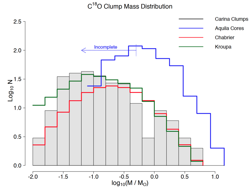
Figure 12: Observed clump mass distribution in the Western Wall molecular cloud plotted as a grey histogram. The blue histogram is the core mass distribution found by Könyves et al. (2015) in Herschel data of the Aquila Rift clouds (their Fig. 16). The red and green histograms correspond to 75 M_⊙ of material distributed among stars with M $<$ 6.31 M_⊙ according to the IMFs of Chabrier (2005) and Kroupa (2001), respectively.

Fig. 12 shows that the clump masses in the Western Wall generally follow the Chabrier (Chabrier, 2005) and Kroupa (Kroupa, 2001) IMFs, with a bit of a deficit at masses just below 1 M_⊙. The lowest clump masses match the Kroupa IMF somewhat better than the Chabrier IMF. As noted above, the number of very low mass ($\lesssim$ 0.05 M_⊙) clumps identified by Gaussclumps depends upon the parameters it uses, with more of these found with a higher number of iterations as the code endeavors to fit Gaussians to non-Gaussian shaped objects. This uncertainty should be kept in mind when evaluating the numbers in the lowest histogram bins in Fig. 12.

Like the IMF, the clump mass distribution in the Western Wall is shifted to lower masses when compared with the core mass distribution in the Aquila Rift clouds. However, our ALMA data resolve structures $\sim$ 4 times smaller than those achieved in the Aquila study (Aquila is $\sim$ 9 times closer than Carina but the spatial resolution of ALMA is 36 times better than the Herschel data used in Aquila). The smallest mass concentrations identified with ALMA would merge into fewer more massive structures at Herschel’s resolution. The effect of instrumental resolution on the properties of clumps extracted from observations has been noted before by several researchers (e.g. Schneider & Brooks, 2004, for molecular observations of Carina). A new CARMA study of C¹⁸O clumps in Orion A taken with a resolution of 3300 au (Takemura et al., 2021) compares more closely with our resolution of 2300 au, and found a relatively flat clump mass function between 0.07M_⊙ and 0.7 M_⊙, similar to that in Fig. 12. Because the distribution of clump masses we find is similar to that of the IMF, the clumps do not necessarily need to evolve further, for example by merging, to become precursors to stellar systems. However, as we will see below, the smallest clumps tend to be unbound gravitationally, implying that some additional processes of fragmentation and merging will be needed to create a typical IMF.

We need to estimate the radius of each clump to find its average density and to assess whether or not the clump is bound gravitationally. Gaussian clumps do not have a fixed radius, but are instead characterized by their standard deviations $\sigma$ along the major and minor axes, and a position angle. Table 2 gives the observed values of the Gaussian sigmas for both the major and minor axes, integrated over the velocity extent of the clump. We do not want to use the sizes within any single velocity slice, as those will underestimate the true size of the clump if any rotation or otherwise structured motion exists within the clump. After correcting for the ALMA beam size (FWHM = 1.0^′′, $\sigma_{res}$ = 0.42^′′), we average the Gaussian clump’s sigmas along the two spatial axes to obtain the spatial size $<\sigma_{R}>$. As most of the mass in a Gaussian clump is contained within a distance of 3-sigma of the center, we adopt the radius of the clump to be R = 3$<\sigma_{R}>$.

The average clump density of H₂ is about $10^{5}$ cm^-3 (top panel of Fig. 13), with a scatter of about a factor of $\sim$ 3 on either side of this value. The data span about an order of magnitude in radius, and have a weak trend in that larger clumps tend to have slightly lower average densities. Most of the clumps are rather oblate in shape, with a median eccentricity of 0.75 for the clumps with masses above the median mass (e.g. Fig. 11). The clump densities in Fig. 13 are on average higher than those in the Aquila Rift and Orion A cores by a factor of $\sim$ 3 (Könyves et al., 2015; Takemura et al., 2021), but these differences are not unexpected given the larger beam sizes used for those studies. Overall, there is nothing extraordinary about the average clump densities in Carina’s Western Wall cloud.

The C¹⁸O clumps in Table 2 show a clear positive correlation between their internal radial velocity dispersions $\sigma_{\rm Vrad}$ and their Masses (bottom panel of Fig. 13). For a constant density clump, M $\sim$ R³, and in virial equilibrium $\sigma_{\rm Vrad}$² $\sim$ M/R. Hence, we expect M $\sim$ $\sigma_{\rm Vrad}^{3}$ for this simple model, shown as a dashed line in the figure. This relationship fits the observations reasonably well, though the scatter is large.

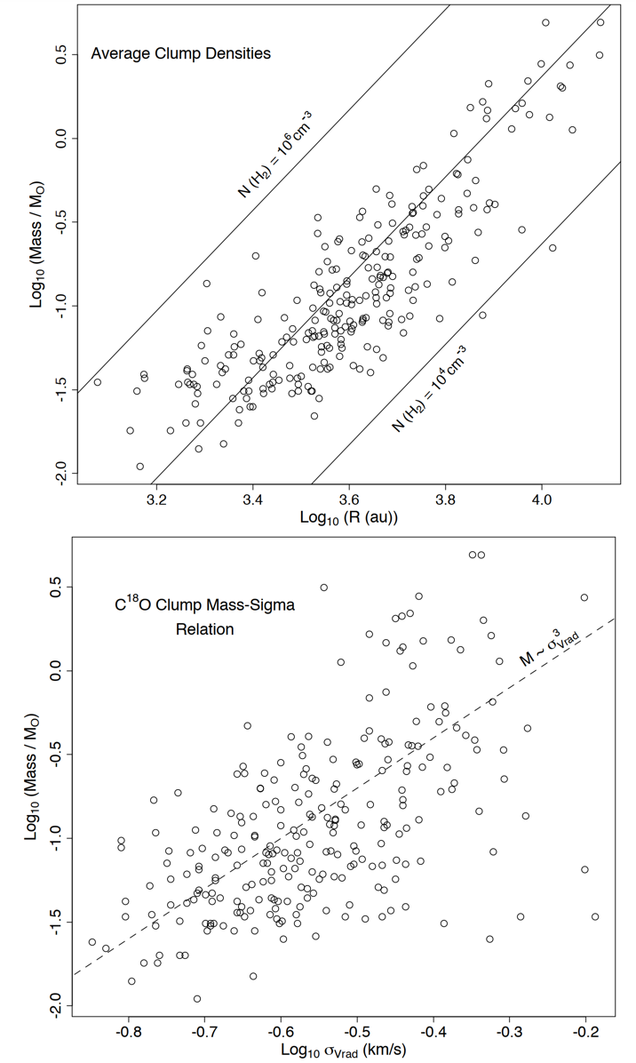
Figure 13: Top: Average densities within C¹⁸O clumps. Bottom: Relationship between the clump mass and the internal velocity dispersion in the C¹⁸O line. The dashed line is what would be expected from a simple virial model for a constant density sphere.

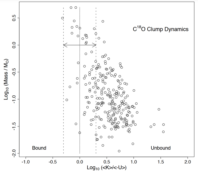
Figure 14: Ratio of the total kinetic energy <K> to the total potential energy <U> for C¹⁸O clumps of different masses. The boundary where log₁₀<K>/$-$<U> = 0 separates unbound clumps from bound clumps. The other two vertical lines indicate factors of two uncertainties about this value. Such uncertainties, can arise from differences in how the mass is distibuted within the clumps and the radius used to define the full extent of the clump.

The gravitational potential energy for a sphere of radius R is $-\xi$GM²/R, where $\xi$ is a constant of order unity that depends upon the radial distribution of mass in the sphere. The value of $\xi$ equals 0.6 for a uniform density sphere and increases as the density becomes more centrally concentrated. For example, $\xi$ = 1.2 for a polytrope with polytropic index $\gamma$ = 1.4, as appropriate for purely diatomic molecular gas. The kinetic energy of the clump is given by <K> = 0.5M<V²>, where <V²> = 3<V${}^{2}_{rad}$> = 3<$\sigma^{2}_{Vrad}$>. Here, V_rad is the radial velocity relative to the mean clump velocity and <$\sigma_{Vrad}$> is the radial velocity sigma corrected for instrumental broadening (instrumental FWHM = 2 channels = 0.28 km s^-1, so $\sigma_{Vinst}$ = 0.12 km s^-1). The criterion for a bound clump then becomes <K> $<$ <$-$U>, or M $>$ 1.5R$\sigma_{Vrad}^{2}$/($\xi$G). To within a factor of order unity, this is the Bonnor-Ebert mass (Bonnor, 1956).

Fig. 14 shows the ratio of kinetic energy to potential energy for the C¹⁸O clumps in our datacube. The heavy-dashed line corresponds to $\xi$ = 1, and the light-dashed lines on either side depict a factor of two error in the value of <K>/<$-$U>. The results show that the most massive clumps congregate near the boundary of stability, while the clumps less massive than $\sim$ 0.5 M_⊙ become progressively less gravitationally bound on average.

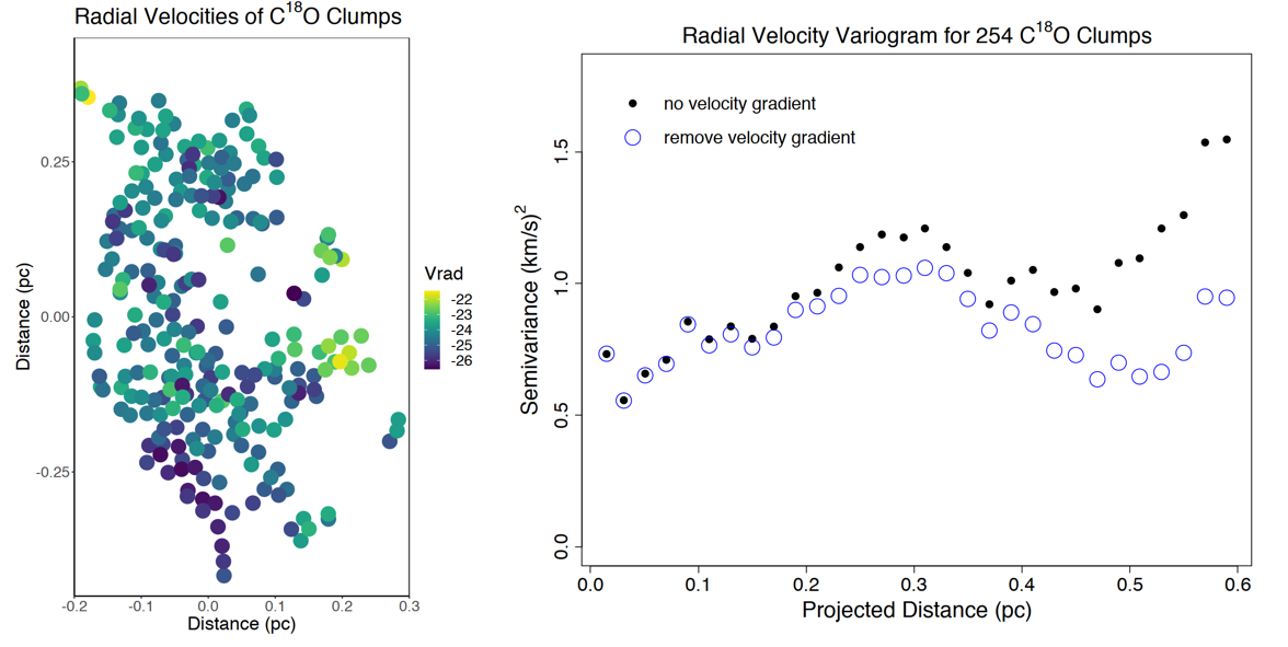
Figure 15: Left: Map of the LSR radial velocities Vrad of the C¹⁸O clumps. The color scale units are km s^-1. Right: Variogram of the C¹⁸O radial velocities, with and without the velocity gradient of the cloud removed (blue circles and black dots, respectively).

The observed line widths in the clumps are wider than expected for thermal broadening of CO, but in most cases the motions within the clumps do not need to be supersonic. The first and third quartiles of the deconvolved C¹⁸O Gaussian $\sigma_{Vrad}$ in the clumps are 0.19 km s^-1 and 0.32 km s^-1, respectively. The isothermal sound speed of pure H₂ gas at 30 K is C_S = 0.42 km s^-1, implying $\sigma_{Cs}$ = C_S/$\gamma^{0.5}$ = 0.35 km s^-1, which is on the order of the observed motions. For reference, the expected thermal $\sigma_{Vrad}$ for C¹⁸O at 30 K is only 0.09 km s^-1. Hence, subsonic turbulence can account for the observed velocity broadening in most clumps, and any nonthermal magnetic broadening will also contribute to the line widths.

4.3 Kinematics Between Clumps

The left side of Fig. 15 shows the clump V_LSR radial velocities across the Western Wall cloud. The radial velocites of our collection of 254 clumps vary between $-$26.59 km s^-1 and $-$21.46 km s^-1, with a median of $-$24.44 km s^-1. There is a small velocity gradient from south to north across the cloud (Sec. 3.2.4, Fig. 3). A good way to assess correlation lengths of spatial data such as these is with a variogram like the one shown on the right side of Fig. 15 (see, e.g., Feigelson, & Babu, 2012, for a description of the mathematics of variograms). In this figure, the variogram calculates the velocity scatter within an annulus of a given projected distance from each point. If there were a preferred correlation length, for example from individual clouds that fragmented into clumps, then the variogram should reveal the characteristic size of the parent clouds.

However, when corrected for the velocity gradient across the cloud, the variogram in Fig. 15 is essentially flat with projected distance, indicating that the velocity scatter from nearby clumps is the same as that for more distant clumps. There is a weak peak at 0.3 pc, and another one at 0.6 pc, but the latter is of low confidence because 0.6 pc is a significant fraction of the size of the entire mapped area. The takeaway here is that once the velocity gradient is removed there are no other significant velocity concentrations present in the clump data.

The typical value of $\sim$ 0.7 km²s^-2 for the semivariance implies 1.4 for the variance, or $\sim$ 1.2 km s^-1 for $\sigma_{Vrad}$. This value is about a factor of three to five times larger than the velocity dispersion within a typical clump. This finding is consistent with the typical core velocity dispersion properties detailed in the models of Chen et al. (2019a), who found markedly smaller velocity dispersions within individual cores as compared with the velocity dispersion of the cloud as a whole. The overall dynamical picture is summarized graphically in Fig. 16.

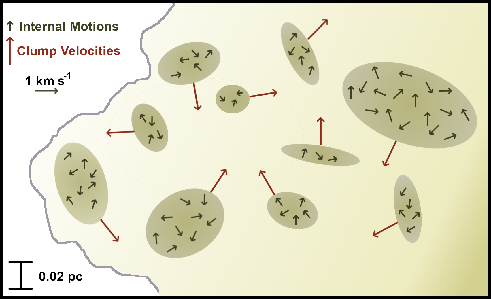
Figure 16: Summary of the observed dynamics of clumps in the Western Wall molecular cloud. The internal velocity dispersions within single clumps, depicted by dark arrows, are on the order of the sound speed in the gas and are larger in the more massive clumps. Motions between clumps, shown as red arrows, are typically 3 $-$ 5 times larger than the sound speed.

5 Discussion

5.1 Are There Protostars in the Western Wall?

In Section 4.2, we found that several of the most massive clumps in Western Wall cloud approach or exceed the threshold to be gravitationally bound. This result raises the question of whether these clumps may already have formed protostars at their centers, which would imply we should uncover them as strong sources of infrared continuum (see, e.g., Dunham et al., 2014).

To investigate this possibility, we searched the standard infrared survey catalogs for point sources over the range of the ALMA map. 2MASS (Skrutskie et al., 2006) detected three point sources within the Western Wall region, but these sources do not overlap with any of our clumps, and are likely to be background objects. Brooks et al. (2001) observed 4.8 GHz continuum along the PDR of the Western Wall cloud, but their maps have a 10-arcminute field of view so it is difficult to compare them with the ALMA data. The one compact source they noted is located well to the north and west of our map. Of the 642 point-like Herschel continuum sources found between 70 $\mu$m and 500 $\mu$m in Carina by Gaczkowski et al. (2013), only J104331.2–593529 and J104331.8–593554 lie within our ALMA field, and neither of these coincides with a C¹⁸O clump. Gaczkowski et al. (2013, see also ()) observed diffuse 160 $\mu$m emission along the Western Wall, but this emission is not clearly associated with a protostar. The H₂ adaptive optics image (Fig. 7; Hartigan et al., 2020) shows over 100 stars visible at 2.12 $\mu$m, but none of these show any obvious relationship with the ALMA C¹⁸O clumps. The lack of far-IR sources in the portion of the Western Wall cloud we mapped with ALMA implies that the clumps we identified in C¹⁸O are starless.

In the last two decades, several theoretical works have calculated the temperature of starless cores as a function of physical parameters such as the gas density, the dust opacity, and the interstellar radiation field (e.g., Evans et al., 2001; Stamatellos & Whitworth, 2003; Stamatellos et al., 2004). In general, these studies found that varying the gas density and dust opacity within reasonable ranges leads to relatively small temperature variations. However, an increase of the external radiation intensity from 1$G_{0}$ to 100$G_{0}$ could double the temperature at the center of a dense core to $\gtrsim$ 20 K (Galli et al., 2002; Lippok et al., 2016). In the Western Wall cloud the radiation field is $\sim$ 3$\times$10⁴ G₀ (Wu et al., 2018), comparable to what is observed in the Orion Nebula, so the observed brightness temperatures in Fig. 4 make sense from a theoretical standpoint without a need to invoke additional internal sources of radiation.

5.2 Effects of External Illumination on the Molecular Gas in the Western Wall Cloud

Our new ALMA maps of the Western Wall cloud have shown that strong external radiation fields affect some characteristics of star-forming regions, while leaving others relatively unchanged. The most obvious effect of radiation occurs along the surface of the PDR, where high-resolution images in H₂ uncover a variety of intriguing structures such as waves, Kelvin-Helmholz shear, and irregular interfaces amplified by shadowing as the gas photoablates from the surface of the cloud. This photoevaporation reduces the lifetime of the molecular cloud, and, in turn, the time available for planets to form within circumstellar disks embedded in this environment. Another obvious effect of the radiation is to increase the overall density of the molecular cloud along the dissociation front, as evidenced by the increased number of C¹⁸O clumps situated near the surface of the cloud compared with the number present in the interior. In this sense, radiation helps to trigger star formation in that it creates conditions immediately behind the front where the densities are closer to those needed for gravitational collapse. Other less-obvious effects of radiation include changing the isotopic CO flux ratio plots in Fig. 5 as discussed in Sec. 3.2.1.

On the other hand, the ALMA data do not reveal any cases where we can clearly point to a new protostar that is forming owing to the compression caused by the radiation front. The C¹⁸O clumps that congregate behind the dissociation front all appear to be starless. Unlike in the southern reaches of the Carina Nebula, we do not observe any pillars jutting out of the Western Wall. There are no instances of long pillars tailing away from the radiation front with a protostar located at the head of the pillar where one might argue that the radiation front helped to confine the protostar laterally after the front moved past the collapsing core. It is possible that magnetic fields play a major role in inhibiting pillar development in the Western Wall, as the morphology of the H₂ image along the curved portion of the PDR immediately facing Trumpler 14 shows a series of relatively smooth ridges Hartigan et al. (2020). Higher internal temperatures for the Western Wall caused by the radiation field may also play a role to inhibit star formation. Our maps do not cover the entire cloud, and studies over a wider field of view may yet uncover protostar activity in this region.

Because our ALMA data have extraordinarily high spatial resolution, we were able to identify clumps that are significantly below the mass cutoff limit of core surveys in many other regions. Nonetheless, as for the previous core survey results, the overall shape of the mass distribution of the C¹⁸O clumps resembles that of the IMF, and the clump densities and internal velocities seem fairly ordinary. There is no clear indication that the fragmentation and merging processes in the Western Wall differ significantly from those in less-exteme environments, despite the fact that the temperatures are higher in this cloud than they are in more quiescent regions.

6 Conclusions

The G287.38-0.62 (Car 1-E) region in the Carina star-forming complex provides an ideal environment to study how strong radiation fields from massive stars influence the observable properties of the molecular clouds in their vicinity. Our program combined ALMA’s 7-m, 12-m, and Total Power arrays to create 1^′′ (0.011 pc) resolution datacubes and continuum maps of ¹²CO, ¹³CO, C¹⁸O, and [C I] over a field of view of $\sim$ 60^′′ $\times$ 80^′′ (0.66 $\times$ 0.88 pc). Situated near the young star cluster Trumpler 14, the Western Wall cloud is the most highly-irradiated structure in the region, though our maps reveal several molecular clouds with different radial velocities that superpose upon the line of sight. At least one of these clouds is part of the Carina complex, so we can compare the Western Wall cloud with a less-irradiated counterpart in the same map.

In agreement with theoretical expectations, there is a clear progression from fluoresced H₂, to [C I], to C¹⁸O with distance into the PDR front of the Western Wall, with spatial offsets between these regions $\sim$ $10^{17}$ cm. Emission from the optically thick ¹²CO line extends across the region, while ¹³CO, [C I] and especially C¹⁸O are more optically thin, and concentrate into clumps and filaments closer to the PDR interface.

The temperature in the Western Wall cloud reaches $\sim$ 80 K in its outer layes, about 20% higher than that within the less-irradiated cloud. As predicted by theoretical models, C¹⁸O must be depleted relative to ¹³CO to explain the observed flux ratios among the CO isotopologues in both clouds. The flux ratios are generally similar between the two clouds, though some systematic differences exist. Dust sizes inferred from continuum measurements at two frequencies are consistent with interstellar grains, with no evidence for grain growth in the Western Wall region. We discovered several bright, compact sources in the CO cubes that may represent disks or outflows from young stars, but these all have velocities significantly different from those in the Western Wall cloud, and so are most likely to be foreground or background objects.

Using a Gaussian fitting algorithm, we identified 254 distinct C¹⁸O clumps in the Western Wall cloud. The mass distribution of these objects is similar to that of the stellar IMF. More massive clumps exhibit higher internal velocity dispersions than less massive clumps do, and the line widths generally follow what is expected from virial equilibrium, with significant scatter. Smaller clumps tend to be weakly unbound, and more massive clumps are more likely to be bound. The average clump density is $\sim$ $10^{5}$ cm^-3 across clumps of all sizes. A typical clump radius is 0.02 pc, or $\sim$ 4 ALMA beam sizes. Clumps tend to be oblate, with a median eccentricity of 0.75 for clumps with masses above the median mass.

The observed line widths in clumps significantly exceed those expected for simple thermal broadening in CO, but can be explained by $\sim$ Mach 1 motions within the clumps in most cases. The variation of velocities between clumps is higher, implying Mach numbers of 3 $-$ 5 for these relative motions. A variogram analysis of the radial velocities of the clumps does not show any characteristic coherent spatial scales among the cores, though there is a velocity gradient of a few km s^-1 north to south across the Western Wall cloud. The ALMA data show no direct evidence for triggering in the Western Wall in that the clumps and cores within the mapped area appear starless, and no pillars are present. However, the densest portion of the cloud lies closest to the PDR, and some of the C¹⁸O emission is flattened along the radiation front.

The extraordinary spatial resolution of ALMA as compared with single dish observations makes it possible to compare molecular maps on the same footing as optical and near-infrared images. This capability shows its true power in a complex region like Carina, where several molecular clouds exist along the line of sight, intricate interface shapes abound, and hundreds of stars are visible within a square parsec. The high spatial resolution of ALMA enables studies of line ratios and kinematics like those presented in this paper that explore scales ranging from a few thousand au to $\sim$ 1 pc in a single cohesive data set. This multi-scale observational capability is an excellent way to inform analogous models as to the main physical properties at work in these environments.

Table 2: Gaussian model fits for C¹⁸O clumps. Column 1: ID number of the clump; Columns 2 and 3: Coordinates; Column 4: V_LSR of the clump; Columns 5 and 6: sigma of the Gaussian clump shape in arcseconds along major and minor axes respectively, summed over velocity and corrected for the 0.47^′′ 1-sigma ALMA beam size; Column 7: Position angle of the Gaussian clump’s major axis on the sky when integrated over velocity; Column 8: Sigma of Gaussian clump dispersion in km/s integrated over the spatial extent of the clump after correcting for the spectral resolution of the observations; Column 9: Peak flux in Jy beam^-1; Column 10: Mass in solar units.

ID	RA (2000.0)	Dec (2000.0)	VLSR	dMax	dMin	PA	Width	Flux	Mass
			(km s-1)	(arcsec)	(arcsec)	(deg)	(km s-1)	(Jky/beam)	(M⊙)
1	10:43:31.64	$-$59:35:38.754	$-$24.804	2.05	1.04	88	0.46	0.93	4.92
2	10:43:30.71	$-$59:35:57.119	$-$24.927	2.77	1.18	118	0.45	0.74	4.93
3	10:43:30.71	$-$59:35:51.174	$-$25.523	1.50	0.92	141	0.36	0.70	2.12
4	10:43:31.77	$-$59:35:43.146	$-$24.348	1.45	0.90	92	0.33	0.64	1.66
5	10:43:30.11	$-$59:35:58.608	$-$25.059	1.67	1.34	168	0.38	0.56	2.79
6	10:43:30.78	$-$59:36:14.024	$-$25.920	1.80	1.05	158	0.37	0.54	2.21
7	10:43:30.82	$-$59:35:28.015	$-$24.123	2.65	1.28	85	0.29	0.52	3.15
8	10:43:31.03	$-$59:35:48.537	$-$24.524	1.22	1.01	90	0.42	0.49	1.53
9	10:43:30.88	$-$59:36:09.897	$-$25.436	1.31	1.09	24	0.34	0.51	1.47
10	10:43:30.18	$-$59:36:07.792	$-$25.092	2.07	1.22	169	0.35	0.47	2.05
11	10:43:31.23	$-$59:35:35.765	$-$24.134	1.22	0.87	44	0.37	0.44	1.07
12	10:43:31.25	$-$59:35:30.799	$-$23.608	0.97	0.88	2	0.33	0.43	0.69
13	10:43:31.23	$-$59:35:53.561	$-$24.749	1.43	0.95	67	0.36	0.42	1.31
14	10:43:31.43	$-$59:35:44.995	$-$24.833	1.96	0.84	85	0.47	0.41	1.62
15	10:43:30.70	$-$59:35:49.172	$-$24.980	1.92	0.96	135	0.36	0.41	1.39
16	10:43:30.88	$-$59:36:03.166	$-$25.354	0.94	0.63	21	0.38	0.38	0.50
17	10:43:31.74	$-$59:35:36.834	$-$24.763	0.76	0.44	155	0.24	0.40	0.20
18	10:43:31.16	$-$59:36:05.457	$-$24.521	1.70	1.00	112	0.39	0.37	1.51
19	10:43:31.61	$-$59:36:01.706	$-$23.382	1.02	0.65	141	0.27	0.35	0.41
20	10:43:31.16	$-$59:36:12.577	$-$25.519	0.80	0.60	93	0.22	0.34	0.24
21	10:43:30.77	$-$59:36:00.291	$-$24.838	2.50	0.85	156	0.46	0.34	2.01
22	10:43:31.16	$-$59:35:40.116	$-$24.508	2.05	1.38	84	0.63	0.34	2.74
23	10:43:31.86	$-$59:35:40.580	$-$24.478	0.87	0.49	81	0.37	0.33	0.27
24	10:43:31.63	$-$59:35:47.997	$-$24.044	1.05	0.76	8	0.48	0.32	0.65
25	10:43:30.64	$-$59:35:31.627	$-$24.236	2.57	0.93	61	0.30	0.32	1.13
26	10:43:29.40	$-$59:35:21.485	$-$23.355	0.78	0.72	177	0.34	0.30	0.37
27	10:43:30.34	$-$59:36:09.265	$-$24.607	0.96	0.70	177	0.27	0.30	0.31
28	10:43:31.14	$-$59:35:55.510	$-$24.524	0.78	0.54	79	0.49	0.30	0.34
29	10:43:30.03	$-$59:36:00.336	$-$25.677	1.60	0.65	149	0.23	0.29	0.47
30	10:43:29.73	$-$59:35:33.006	$-$24.309	1.20	1.01	134	0.34	0.29	0.75
31	10:43:30.28	$-$59:35:52.879	$-$25.736	1.03	0.63	8	0.43	0.29	0.46
32	10:43:30.54	$-$59:36:12.143	$-$25.451	1.03	0.62	27	0.23	0.29	0.24
33	10:43:30.69	$-$59:35:23.617	$-$24.376	1.37	0.76	108	0.41	0.29	0.62
34	10:43:30.55	$-$59:36:13.531	$-$26.438	1.02	0.54	145	0.17	0.28	0.17
35	10:43:30.56	$-$59:35:33.370	$-$23.815	0.87	0.63	41	0.27	0.26	0.24
36	10:43:29.40	$-$59:35:25.062	$-$23.623	1.00	0.78	58	0.37	0.26	0.36
37	10:43:30.97	$-$59:35:46.556	$-$24.298	0.91	0.82	78	0.25	0.26	0.28
38	10:43:30.14	$-$59:36:03.509	$-$25.191	2.21	0.94	17	0.43	0.26	1.34
39	10:43:30.50	$-$59:35:58.547	$-$24.326	1.10	0.75	134	0.32	0.26	0.40
40	10:43:31.02	$-$59:35:29.477	$-$23.656	0.87	0.48	71	0.15	0.25	0.10
41	10:43:30.63	$-$59:36:07.488	$-$25.579	1.19	0.94	2	0.29	0.25	0.38
42	10:43:30.44	$-$59:36:16.615	$-$26.216	0.74	0.62	148	0.27	0.24	0.16
43	10:43:26.88	$-$59:36:09.501	$-$25.230	0.74	0.52	176	0.21	0.24	0.11
44	10:43:29.80	$-$59:36:28.907	$-$25.243	1.08	0.71	56	0.34	0.24	0.39
45	10:43:31.18	$-$59:35:32.735	$-$24.230	1.25	0.63	9	0.22	0.24	0.27
46	10:43:31.43	$-$59:36:02.974	$-$23.853	1.00	0.54	25	0.26	0.23	0.20
47	10:43:31.12	$-$59:36:10.105	$-$25.803	1.37	0.47	113	0.39	0.24	0.27
48	10:43:30.55	$-$59:35:47.066	$-$24.616	1.33	0.81	146	0.40	0.24	0.61
49	10:43:30.43	$-$59:35:53.745	$-$24.733	1.69	0.97	163	0.49	0.23	1.14
50	10:43:30.49	$-$59:35:26.901	$-$23.579	1.29	0.69	70	0.27	0.23	0.35
51	10:43:30.91	$-$59:35:26.376	$-$24.594	0.87	0.65	143	0.24	0.23	0.20
52	10:43:31.16	$-$59:35:24.412	$-$23.747	1.03	0.86	170	0.41	0.23	0.50
53	10:43:29.57	$-$59:35:37.227	$-$24.905	0.81	0.55	168	0.27	0.22	0.18
54	10:43:31.98	$-$59:36:01.642	$-$23.630	0.78	0.62	91	0.37	0.22	0.25
55	10:43:30.99	$-$59:35:51.958	$-$24.712	0.86	0.49	134	0.30	0.22	0.16
56	10:43:31.69	$-$59:35:40.166	$-$25.586	0.76	0.41	141	0.22	0.22	0.09
57	10:43:30.84	$-$59:35:36.921	$-$23.568	0.89	0.60	4	0.45	0.22	0.34
58	10:43:31.61	$-$59:36:04.859	$-$24.526	0.78	0.60	175	0.25	0.21	0.17
59	10:43:32.33	$-$59:35:18.473	$-$22.183	0.98	0.61	108	0.39	0.21	0.30
60	10:43:31.42	$-$59:35:39.024	$-$24.743	0.59	0.46	85	0.53	0.21	0.14
61	10:43:29.63	$-$59:36:08.484	$-$24.415	0.94	0.84	92	0.37	0.20	0.36
62	10:43:31.54	$-$59:36:00.121	$-$24.095	0.83	0.70	170	0.34	0.20	0.25
63	10:43:29.51	$-$59:36:05.349	$-$25.600	1.18	0.81	128	0.33	0.20	0.44
64	10:43:30.17	$-$59:36:17.875	$-$26.385	0.78	0.65	89	0.22	0.20	0.14
65	10:43:27.55	$-$59:35:58.912	$-$22.465	1.07	0.81	94	0.29	0.20	0.30
66	10:43:29.65	$-$59:35:23.098	$-$24.397	1.06	0.67	53	0.32	0.19	0.28
67	10:43:31.14	$-$59:35:44.848	$-$25.034	1.25	0.63	75	0.53	0.20	0.45
68	10:43:30.09	$-$59:35:27.107	$-$23.026	1.04	0.56	9	0.30	0.18	0.21
69	10:43:28.90	$-$59:36:00.208	$-$25.128	1.64	0.68	154	0.41	0.17	0.56
70	10:43:30.92	$-$59:36:05.661	$-$24.037	0.89	0.56	69	0.23	0.17	0.14
71	10:43:30.95	$-$59:36:08.944	$-$24.809	0.95	0.39	99	0.25	0.18	0.09
72	10:43:27.84	$-$59:35:58.018	$-$22.936	0.85	0.77	88	0.29	0.18	0.20
73	10:43:31.89	$-$59:35:44.640	$-$24.468	0.69	0.43	131	0.24	0.17	0.07
74	10:43:31.56	$-$59:35:55.610	$-$23.623	0.91	0.48	56	0.49	0.17	0.23
75	10:43:31.03	$-$59:36:03.548	$-$24.768	1.30	0.96	59	0.45	0.17	0.39
76	10:43:31.67	$-$59:35:22.272	$-$24.066	0.92	0.84	90	0.35	0.17	0.29
77	10:43:29.83	$-$59:36:03.646	$-$22.839	0.77	0.54	7	0.29	0.17	0.13
78	10:43:28.07	$-$59:35:45.473	$-$23.748	0.90	0.75	168	0.20	0.17	0.15
79	10:43:31.54	$-$59:35:36.100	$-$25.732	0.79	0.44	50	0.32	0.17	0.12
80	10:43:31.37	$-$59:35:51.233	$-$23.449	0.75	0.69	85	0.42	0.16	0.21
81	10:43:31.26	$-$59:35:27.015	$-$23.767	0.79	0.57	29	0.23	0.16	0.10
82	10:43:31.32	$-$59:35:59.581	$-$24.764	1.43	0.62	130	0.25	0.16	0.22
83	10:43:29.96	$-$59:36:08.892	$-$24.451	0.79	0.40	17	0.18	0.16	0.06
84	10:43:30.88	$-$59:35:24.546	$-$23.601	0.73	0.45	91	0.17	0.16	0.05
85	10:43:29.95	$-$59:35:56.818	$-$25.117	0.55	0.38	43	0.17	0.16	0.04
86	10:43:30.86	$-$59:35:54.685	$-$23.835	1.38	1.09	93	0.26	0.15	0.40
87	10:43:29.33	$-$59:36:04.085	$-$24.782	1.01	0.88	83	0.28	0.15	0.23
88	10:43:31.63	$-$59:35:34.984	$-$23.753	1.87	0.51	49	0.18	0.16	0.19
89	10:43:29.60	$-$59:36:06.708	$-$24.683	1.72	0.63	172	0.32	0.15	0.28
90	10:43:30.44	$-$59:36:05.644	$-$24.924	1.64	0.40	12	0.30	0.15	0.13
91	10:43:30.33	$-$59:35:29.511	$-$23.474	0.89	0.74	78	0.24	0.15	0.16
92	10:43:29.88	$-$59:35:26.015	$-$23.809	1.03	0.77	177	0.41	0.14	0.27
93	10:43:30.29	$-$59:35:56.709	$-$24.015	1.30	0.76	111	0.24	0.15	0.24
94	10:43:29.91	$-$59:36:21.853	$-$26.078	0.97	0.63	88	0.25	0.15	0.15
95	10:43:30.25	$-$59:35:26.132	$-$23.636	0.76	0.56	0	0.34	0.14	0.13
96	10:43:27.72	$-$59:35:43.213	$-$22.039	0.94	0.52	145	0.22	0.14	0.10
97	10:43:28.69	$-$59:36:16.452	$-$24.781	1.17	0.85	134	0.27	0.14	0.26
98	10:43:30.07	$-$59:35:29.280	$-$24.453	1.19	0.94	92	0.38	0.14	0.35
99	10:43:31.39	$-$59:35:53.887	$-$25.135	0.92	0.47	109	0.34	0.14	0.09
100	10:43:27.98	$-$59:35:40.129	$-$24.253	0.77	0.53	143	0.18	0.14	0.07
101	10:43:29.44	$-$59:35:32.294	$-$24.602	0.75	0.57	44	0.35	0.14	0.12
102	10:43:29.77	$-$59:35:34.826	$-$24.429	1.07	0.58	4	0.19	0.14	0.11
103	10:43:29.89	$-$59:35:34.208	$-$26.379	0.79	0.57	1	0.29	0.13	0.12
104	10:43:30.65	$-$59:35:34.548	$-$24.563	1.07	0.45	3	0.34	0.14	0.12
105	10:43:31.02	$-$59:35:34.340	$-$24.439	0.94	0.39	155	0.28	0.13	0.06
106	10:43:31.36	$-$59:35:24.205	$-$23.328	1.04	0.57	100	0.28	0.13	0.15
107	10:43:29.35	$-$59:35:22.390	$-$24.099	0.86	0.60	24	0.23	0.13	0.10
108	10:43:31.46	$-$59:36:05.723	$-$24.447	0.66	0.57	3	0.19	0.13	0.06
109	10:43:28.21	$-$59:36:00.033	$-$25.138	1.20	0.48	10	0.30	0.13	0.15
110	10:43:29.19	$-$59:35:26.830	$-$23.425	0.72	0.58	60	0.20	0.12	0.07
111	10:43:29.48	$-$59:35:59.571	$-$25.406	0.97	0.62	50	0.36	0.12	0.17
112	10:43:27.59	$-$59:35:56.712	$-$21.962	0.74	0.64	137	0.38	0.12	0.13
113	10:43:30.66	$-$59:35:41.234	$-$24.939	0.71	0.39	22	0.30	0.13	0.06
114	10:43:29.72	$-$59:36:02.703	$-$25.934	0.85	0.54	134	0.21	0.12	0.08
115	10:43:31.76	$-$59:35:37.737	$-$25.784	0.68	0.38	61	0.19	0.13	0.04
116	10:43:31.10	$-$59:35:59.506	$-$23.285	1.54	0.87	129	0.35	0.12	0.38
117	10:43:30.73	$-$59:36:00.098	$-$23.902	1.30	0.55	119	0.17	0.12	0.11
118	10:43:30.86	$-$59:35:49.359	$-$23.446	0.84	0.61	177	0.27	0.12	0.11
119	10:43:29.18	$-$59:36:07.288	$-$23.954	1.30	0.62	18	0.22	0.12	0.14
120	10:43:31.30	$-$59:35:22.824	$-$23.952	0.88	0.69	22	0.26	0.12	0.11
121	10:43:28.85	$-$59:36:13.545	$-$24.950	0.81	0.77	88	0.28	0.12	0.13
122	10:43:29.57	$-$59:36:03.513	$-$23.458	1.26	0.59	51	0.41	0.12	0.19
123	10:43:28.08	$-$59:35:41.920	$-$22.608	0.85	0.59	143	0.24	0.12	0.08
124	10:43:27.38	$-$59:35:54.264	$-$22.623	0.96	0.65	114	0.19	0.11	0.08
125	10:43:30.17	$-$59:36:01.501	$-$24.857	1.07	0.44	175	0.20	0.11	0.07
126	10:43:31.94	$-$59:36:02.057	$-$24.653	0.74	0.57	82	0.25	0.11	0.08
127	10:43:27.96	$-$59:36:20.728	$-$24.595	0.98	0.66	9	0.36	0.11	0.16
128	10:43:29.29	$-$59:35:31.207	$-$24.611	0.54	0.47	4	0.22	0.11	0.04
129	10:43:29.09	$-$59:35:28.536	$-$23.599	0.72	0.42	172	0.20	0.11	0.05
130	10:43:30.09	$-$59:35:57.785	$-$24.770	0.69	0.37	116	0.52	0.11	0.03
131	10:43:29.73	$-$59:35:31.599	$-$25.088	0.82	0.64	111	0.21	0.11	0.08
132	10:43:31.65	$-$59:35:20.603	$-$24.460	0.66	0.45	52	0.33	0.11	0.07
133	10:43:30.23	$-$59:35:36.145	$-$23.644	1.00	0.66	155	0.42	0.11	0.20
134	10:43:30.85	$-$59:36:07.713	$-$25.265	0.60	0.42	71	0.26	0.11	0.03
135	10:43:30.75	$-$59:36:02.023	$-$23.009	0.86	0.51	152	0.27	0.11	0.09
136	10:43:27.74	$-$59:35:54.436	$-$22.761	0.95	0.70	83	0.25	0.11	0.12
137	10:43:30.01	$-$59:35:37.248	$-$24.254	0.96	0.80	81	0.22	0.10	0.12
138	10:43:30.90	$-$59:35:37.596	$-$24.136	0.61	0.40	134	0.27	0.10	0.04
139	10:43:28.72	$-$59:36:06.324	$-$23.923	0.78	0.62	81	0.24	0.10	0.07
140	10:43:30.08	$-$59:36:10.929	$-$25.120	0.85	0.71	44	0.29	0.10	0.12
141	10:43:28.87	$-$59:35:37.141	$-$25.102	0.93	0.62	22	0.46	0.10	0.14
142	10:43:29.49	$-$59:36:10.097	$-$24.959	1.15	0.65	3	0.33	0.10	0.16
143	10:43:29.84	$-$59:36:24.636	$-$26.091	0.85	0.50	93	0.25	0.10	0.07
144	10:43:31.42	$-$59:35:33.319	$-$24.091	0.66	0.49	115	0.20	0.10	0.05
145	10:43:30.48	$-$59:35:46.647	$-$25.645	0.86	0.66	173	0.21	0.10	0.09
146	10:43:31.30	$-$59:35:38.633	$-$23.573	1.24	0.41	32	0.27	0.10	0.07
147	10:43:30.46	$-$59:36:02.704	$-$25.793	0.72	0.48	81	0.22	0.10	0.04
148	10:43:29.76	$-$59:35:52.963	$-$25.097	1.58	0.85	140	0.44	0.10	0.41
149	10:43:26.75	$-$59:36:07.963	$-$23.755	0.86	0.45	30	0.16	0.10	0.03
150	10:43:28.48	$-$59:36:01.407	$-$25.289	1.17	0.53	135	0.30	0.09	0.13
151	10:43:28.50	$-$59:35:59.033	$-$24.969	0.57	0.49	8	0.26	0.09	0.04
152	10:43:30.60	$-$59:36:10.255	$-$26.273	0.78	0.61	21	0.26	0.10	0.08
153	10:43:29.53	$-$59:36:05.532	$-$24.104	0.78	0.64	114	0.32	0.09	0.07
154	10:43:29.93	$-$59:36:04.300	$-$23.332	0.62	0.47	147	0.27	0.09	0.05
155	10:43:29.39	$-$59:36:01.568	$-$25.595	1.08	0.75	51	0.36	0.09	0.19
156	10:43:26.73	$-$59:36:06.366	$-$23.746	0.66	0.50	155	0.18	0.09	0.03
157	10:43:27.25	$-$59:35:58.501	$-$22.659	1.11	0.66	82	0.20	0.09	0.09
158	10:43:30.92	$-$59:35:41.714	$-$24.115	0.79	0.42	147	0.26	0.09	0.06
159	10:43:30.37	$-$59:35:46.092	$-$24.109	1.06	0.54	132	0.26	0.09	0.10
160	10:43:28.40	$-$59:36:20.680	$-$23.602	0.76	0.63	91	0.36	0.09	0.11
161	10:43:31.12	$-$59:35:46.912	$-$26.098	0.87	0.62	134	0.29	0.09	0.11
162	10:43:28.61	$-$59:36:03.709	$-$24.924	0.74	0.61	95	0.32	0.09	0.08
163	10:43:29.28	$-$59:35:37.324	$-$24.779	0.71	0.46	158	0.48	0.09	0.08
164	10:43:28.84	$-$59:36:17.273	$-$25.266	0.75	0.45	143	0.19	0.09	0.04
165	10:43:27.96	$-$59:35:39.623	$-$22.969	0.83	0.67	149	0.24	0.09	0.08
166	10:43:29.81	$-$59:36:26.860	$-$25.771	0.64	0.45	53	0.24	0.09	0.04
167	10:43:29.85	$-$59:35:30.037	$-$24.461	0.91	0.45	64	0.24	0.09	0.06
168	10:43:27.96	$-$59:36:19.998	$-$23.457	0.78	0.62	44	0.31	0.09	0.09
169	10:43:28.87	$-$59:35:31.328	$-$23.801	0.81	0.51	61	0.26	0.09	0.07
170	10:43:29.70	$-$59:35:27.797	$-$24.126	0.90	0.62	176	0.37	0.08	0.12
171	10:43:28.40	$-$59:35:48.919	$-$25.436	0.68	0.51	145	0.23	0.09	0.05
172	10:43:27.75	$-$59:35:57.981	$-$21.633	0.75	0.59	134	0.21	0.09	0.06
173	10:43:31.35	$-$59:35:30.704	$-$23.127	0.62	0.45	76	0.34	0.08	0.03
174	10:43:30.31	$-$59:36:13.278	$-$26.250	0.79	0.62	170	0.29	0.08	0.06
175	10:43:28.56	$-$59:35:48.111	$-$26.586	0.50	0.46	44	0.35	0.08	0.04
176	10:43:29.19	$-$59:36:11.067	$-$24.959	0.87	0.64	134	0.29	0.08	0.08
177	10:43:27.84	$-$59:35:42.698	$-$24.280	0.60	0.50	178	0.14	0.08	0.02
178	10:43:28.45	$-$59:36:23.864	$-$23.771	0.64	0.49	57	0.28	0.08	0.05
179	10:43:30.24	$-$59:36:04.331	$-$24.055	2.33	0.87	171	0.28	0.08	0.22
180	10:43:28.61	$-$59:36:22.207	$-$25.418	0.71	0.62	173	0.23	0.08	0.05
181	10:43:30.37	$-$59:35:33.977	$-$24.440	0.76	0.53	69	0.34	0.08	0.07
182	10:43:29.86	$-$59:35:49.328	$-$23.632	0.65	0.58	179	0.38	0.07	0.07
183	10:43:30.04	$-$59:36:02.124	$-$24.422	0.92	0.47	166	0.31	0.08	0.07
184	10:43:30.48	$-$59:35:59.845	$-$23.751	1.11	0.63	2	0.22	0.08	0.07
185	10:43:30.83	$-$59:35:22.508	$-$23.597	1.71	0.68	151	0.15	0.08	0.09
186	10:43:31.81	$-$59:35:21.667	$-$23.275	0.61	0.43	171	0.24	0.07	0.04
187	10:43:32.00	$-$59:36:00.095	$-$25.106	1.80	0.98	100	0.32	0.08	0.28
188	10:43:30.54	$-$59:36:01.414	$-$26.274	0.96	0.55	24	0.16	0.08	0.04
189	10:43:30.45	$-$59:35:28.837	$-$24.929	0.78	0.55	25	0.35	0.08	0.06
190	10:43:29.84	$-$59:35:28.454	$-$24.968	0.69	0.64	4	0.20	0.07	0.05
191	10:43:30.00	$-$59:35:34.039	$-$25.609	0.72	0.65	7	0.36	0.07	0.07
192	10:43:28.17	$-$59:36:02.992	$-$25.127	0.65	0.48	150	0.22	0.07	0.04
193	10:43:30.41	$-$59:35:30.020	$-$25.932	1.19	0.42	107	0.21	0.07	0.06
194	10:43:28.88	$-$59:35:28.749	$-$25.422	0.96	0.69	137	0.24	0.07	0.09
195	10:43:30.41	$-$59:35:31.170	$-$24.790	0.66	0.53	44	0.22	0.07	0.04
196	10:43:30.26	$-$59:35:56.592	$-$23.387	1.02	0.63	21	0.24	0.07	0.08
197	10:43:30.95	$-$59:35:20.255	$-$24.442	0.65	0.39	112	0.17	0.07	0.02
198	10:43:30.10	$-$59:35:31.372	$-$23.463	0.73	0.67	179	0.28	0.07	0.06
199	10:43:28.91	$-$59:35:59.111	$-$24.434	0.77	0.48	111	0.27	0.07	0.04
200	10:43:29.65	$-$59:36:19.842	$-$25.444	1.24	0.84	88	0.27	0.07	0.14
201	10:43:30.25	$-$59:35:46.140	$-$25.778	0.60	0.45	83	0.32	0.07	0.03
202	10:43:29.08	$-$59:35:59.030	$-$23.786	1.04	0.61	70	0.26	0.06	0.08
203	10:43:28.48	$-$59:36:02.523	$-$26.095	0.70	0.42	163	0.20	0.07	0.03
204	10:43:29.20	$-$59:35:45.345	$-$24.596	0.77	0.44	147	0.17	0.07	0.03
205	10:43:32.10	$-$59:35:54.949	$-$23.786	0.67	0.45	127	0.34	0.06	0.05
206	10:43:30.53	$-$59:36:03.120	$-$23.420	0.81	0.63	26	0.31	0.07	0.07
207	10:43:29.29	$-$59:36:18.435	$-$25.588	1.11	0.86	53	0.18	0.06	0.08
208	10:43:28.11	$-$59:35:56.623	$-$23.102	0.88	0.62	108	0.30	0.06	0.08
209	10:43:30.85	$-$59:35:41.846	$-$25.468	0.91	0.47	116	0.20	0.07	0.04
210	10:43:29.63	$-$59:35:29.354	$-$24.446	0.62	0.49	50	0.25	0.06	0.03
211	10:43:31.58	$-$59:35:46.144	$-$23.278	0.79	0.57	159	0.24	0.07	0.06
212	10:43:30.45	$-$59:36:17.447	$-$25.765	0.79	0.39	130	0.22	0.06	0.03
213	10:43:29.74	$-$59:35:41.147	$-$22.789	0.51	0.44	9	0.17	0.06	0.02
214	10:43:28.30	$-$59:36:22.158	$-$23.282	0.78	0.56	26	0.37	0.06	0.07
215	10:43:29.96	$-$59:36:18.443	$-$26.251	0.72	0.57	80	0.25	0.06	0.04
216	10:43:30.51	$-$59:35:55.600	$-$23.116	0.70	0.47	163	0.34	0.06	0.05
217	10:43:30.66	$-$59:35:42.363	$-$24.120	0.70	0.48	62	0.23	0.06	0.03
218	10:43:29.26	$-$59:35:59.906	$-$25.437	0.74	0.42	131	0.31	0.06	0.04
219	10:43:28.95	$-$59:35:54.749	$-$23.609	0.87	0.66	47	0.28	0.06	0.06
220	10:43:32.08	$-$59:35:51.953	$-$24.112	0.69	0.39	50	0.37	0.06	0.04
221	10:43:28.92	$-$59:36:07.849	$-$23.627	0.89	0.66	61	0.18	0.06	0.04
222	10:43:29.09	$-$59:36:16.425	$-$25.111	0.78	0.62	113	0.27	0.06	0.05
223	10:43:27.96	$-$59:35:55.725	$-$22.304	0.69	0.61	110	0.15	0.06	0.02
224	10:43:29.13	$-$59:35:38.040	$-$25.110	0.68	0.42	24	0.17	0.06	0.02
225	10:43:28.01	$-$59:35:59.159	$-$22.614	0.64	0.43	113	0.30	0.06	0.03
226	10:43:30.68	$-$59:35:53.313	$-$24.278	0.66	0.38	42	0.65	0.06	0.03
227	10:43:29.32	$-$59:36:12.854	$-$23.789	0.77	0.59	170	0.25	0.05	0.04
228	10:43:29.83	$-$59:35:59.485	$-$23.616	1.09	0.64	10	0.29	0.06	0.08
229	10:43:28.65	$-$59:36:01.780	$-$24.436	0.76	0.60	172	0.23	0.05	0.04
230	10:43:28.98	$-$59:36:14.733	$-$24.443	0.79	0.47	135	0.23	0.05	0.04
231	10:43:31.69	$-$59:35:25.539	$-$23.613	0.64	0.43	49	0.16	0.05	0.01
232	10:43:30.16	$-$59:36:14.880	$-$25.420	0.99	0.59	8	0.24	0.05	0.06
233	10:43:29.47	$-$59:36:07.758	$-$23.455	0.82	0.50	74	0.20	0.05	0.03
234	10:43:29.68	$-$59:35:37.741	$-$24.119	0.88	0.48	42	0.23	0.05	0.03
235	10:43:28.55	$-$59:35:56.231	$-$22.796	0.87	0.73	2	0.20	0.05	0.05
236	10:43:32.08	$-$59:35:56.719	$-$24.116	0.68	0.56	34	0.29	0.05	0.04
237	10:43:30.20	$-$59:35:34.021	$-$25.274	0.66	0.55	90	0.63	0.05	0.07
238	10:43:29.88	$-$59:36:15.442	$-$24.788	0.70	0.55	169	0.25	0.05	0.04
239	10:43:32.20	$-$59:35:19.751	$-$21.458	0.50	0.45	175	0.20	0.05	0.01
240	10:43:30.35	$-$59:35:28.017	$-$25.759	0.61	0.44	75	0.28	0.05	0.03
241	10:43:29.97	$-$59:35:32.070	$-$24.103	0.76	0.43	16	0.41	0.05	0.03
242	10:43:28.84	$-$59:35:57.535	$-$23.288	0.86	0.60	114	0.21	0.05	0.04
243	10:43:30.92	$-$59:36:11.429	$-$26.446	0.82	0.40	161	0.20	0.05	0.03
244	10:43:30.28	$-$59:36:10.551	$-$24.120	0.71	0.40	119	0.19	0.05	0.02
245	10:43:30.70	$-$59:36:04.747	$-$23.289	0.73	0.47	12	0.26	0.05	0.04
246	10:43:30.17	$-$59:36:19.546	$-$25.769	0.74	0.52	97	0.20	0.05	0.03
247	10:43:29.16	$-$59:35:37.835	$-$24.104	0.72	0.52	29	0.21	0.05	0.03
248	10:43:31.63	$-$59:35:47.525	$-$22.793	0.64	0.48	167	0.25	0.05	0.03
249	10:43:31.25	$-$59:36:03.136	$-$24.114	0.65	0.48	82	0.47	0.05	0.03
250	10:43:27.93	$-$59:35:42.927	$-$22.447	0.63	0.48	63	0.18	0.05	0.02
251	10:43:28.21	$-$59:36:02.033	$-$25.607	0.78	0.52	94	0.20	0.05	0.03
252	10:43:28.57	$-$59:35:54.036	$-$23.115	0.65	0.53	72	0.25	0.05	0.03
253	10:43:32.31	$-$59:35:19.252	$-$23.117	0.76	0.37	111	0.23	0.05	0.01
254	10:43:30.69	$-$59:35:42.455	$-$25.781	0.71	0.57	114	0.25	0.05	0.03

Appendix A Summary of the observations

Table 3 lists the main properties of ALMA interferometric observations reported in this paper, including the frequency bands (1), the antenna array (2), the observation dates (3), the complex gain calibrator (4), bandpass calibrators (5), and the maximum (6) and minimum (7) antenna baselines.

Table 3: Summary of the Interferometric Observations

Band	Array	Date	Gain cal.	Bandpass cal.	Max. Baseline	Min. Baseline
(1)	(2)	(3)	(4)	(5)	(6)	(7)
6	12-m	19-Dec-2015	J1047-6217	J1107-4449	6300m	15.1m
		02-Mar-2016	J1047-6217	J1107-4449	390.0m	15.2m
		17-Mar-2016	J1047-6217	J1107-4449	460.0m	15.2m
6	7-m	28-Jun-2016	J1147-6753	J0854+2006	49.0m	8.8m
		30-Jun-2016	J1147-6753	J0854+2006	43.2m	8.8m
		30-Jun-2016	J1147-6753	J1058+0133	43.2m	8.8m
		30-Jun-2016	J1147-6753	J1427-4206	43.2m	8.8m
8	12-m	19-Dec-2015	J0490-6107	J1256-0547	6300m	15.1m
8	7-m	09-Aug-2016	J1047-6217	J0522-3627	45.0m	8.9m
		20-Aug-2016	J1047-6217	J1256-0547	45.0m	8.9m
		21-Aug-2016	J1047-6217	J1256-0547	45.0m	8.9m
		25-Aug-2016	J1047-6217	J1256-0547	45.0m	8.9m
		07-Sep-2016	J1047-6217	J0522-3627	45.0m	8.9m
		08-Sep-2016	J1047-6217	J1256-0547	45.0m	8.9m

Appendix B Combining single-dish and interferometric data

In this section we describe the procedure followed to combine single-dish and interferometric ALMA data. As a preliminary step, we independently imaged 12-m and 7-m array observations of the targeted emission lines. This step is not necessary for combining the data but it provides images of the high spatial frequency components of the emission that can be compared to the combined images. All the images discussed in this section were produced using the task TCLEAN provided in version 5.6.0 of the CASA package.

The best practice for combining single-dish and interferometric data is matter of debate. Several techniques have been proposed, including combining data before, during, or after deconvolution (see Koda et al., 2019, for a recent review). In this paper, we combined interferometric and single-dish data in the Fourier space before deconvolution using the publicly available Total Power to Visibilities (TP2VIS) algorithm presented in Koda et al. (2019). This method requires deconvolving the single-dish image with the single-dish beam to obtain an infinite resolution model for the emission. This model is then Fourier-transformed to obtain a set of “single-dish” visibilities which are concatenated to the interferometric visibilities and imaged using a standard CLEAN algorithms.

The publicly available version of TP2VIS performs the deconvolution of single-dish images by Fourier-transforming them and dividing the resulting visibilities by the Fourier transform of the synthesized beam. We find that this direct approach to deconvolution does not work well with our data because the line emission extends to the edge of the image field in most of the channels. In such cases, the Fourier transform of a single-dish image acquires strong high frequency components owing to the sharp cutoff of the emission at the image edges. TP2VIS provides a few tapering options to mitigate this issue but none of them led to acceptable results for this data set.

Instead, we deconvolved the single-dish data using an algorithm similar to CLEAN. We performed the decolvolution in the image plane by subtracting point source components. The model image is then Fourier transformed using TP2VIS. The resulting visibilties are combined to the interferometric data and imaged using TCLEAN. We checked the fidelity of the single-dish image deconvolution by re-imaging the calculated single-dish visibilities using TCLEAN and comparing the resulting images to the original single-dish maps. In general, we find that the final images differ from the original images only by a few percent.

Appendix C Optical Depth Calculations

This section calculates the optical depth at line center for a few transitions of interest in PDRs and molecular clouds, assuming standard solar abundances (Asplund et al., 2009) and a thermal broadening profile for a H-column density of $2.7\times 10^{21}$ cm^-2, which corresponds to a visual extinction A_V = 1 (Liszt, 2014). The derivation largely follows that of Chapter 10 of Rybicki & Lightman (1979).

The optical depth $\tau_{\nu}$ at frequency $\nu$ is related to the differential path length $dl$ and the opacity $\alpha_{\nu}$ via $d\tau_{\nu}$ = $\alpha_{\nu}dl$, so for a uniform gas with constant path length $L$, the optical depth integrated along the line of sight becomes

$$\tau_{\nu}=\alpha_{\nu}L$$ (C1)

The opacity is related to the Einstein B coefficients between the upper level (denoted by 2) and lower level (denoted by 1), and their corresponding number densities $n_{1}$ and $n_{2}$ via

$$\alpha_{\nu}={\frac{h\nu}{4\pi}\left[n_{1}B_{12}-n_{2}B_{21}\right]\phi(\nu)}$$ (C2)

where the normalized line profile $\phi(\nu)$ for thermal broadening is

$$\phi(\nu)=\frac{1}{\Delta\nu_{D}\sqrt{\pi}}e^{-\left[(\nu-\nu_{\circ})^{2}/(\Delta\nu_{D})^{2}\right]}$$ (C3)

and

$$\Delta\nu_{D}=\frac{\nu_{\circ}}{c}\sqrt{\frac{2kT}{m}}$$ (C4)

is the Doppler broadening coefficient. Here, $\nu_{\circ}$ is the frequency of the transition at line center, m is the mass of the atom or molecule, and k is Boltzman’s constant and T is the temperature.

Using the Einstein relations

$$A_{21}=\frac{2h\nu^{3}}{c^{2}}B_{21}\ ;\ B_{21}=\frac{g_{1}}{g_{2}}B_{12}$$ (C5)

we can rewrite the term inside the brackets in Equation C2 as

$$n_{1}B_{12}-n_{2}B_{21}=\frac{g_{2}n_{1}A_{21}c^{2}}{2g_{1}h\nu^{3}}{\left[1-\eta e^{-{h\nu/kT}}\right]}$$ (C6)

where we define

$$\eta=\left(\frac{n_{2}}{n_{1}}\right)\bigg{/}\left(\frac{n_{2}}{n_{1}}\right)_{LTE}$$ (C7)

and

$$\left(\frac{n_{2}}{n_{1}}\right)_{LTE}=\ \ \frac{g_{2}}{g_{1}}{\rm e}^{-{h\nu/kT}}$$ (C8)

Defining

$$S=1-\eta e^{-{h\nu/kT}}$$ (C9)

and combining equations C1, C2, C3, C4, C6 and C9 leads to

$$\tau_{\circ}=\frac{\lambda^{3}A_{21}g_{2}}{8\pi g_{1}}\left(\frac{m}{2\pi kT}\right)^{\frac{1}{2}}S{\rm N}_{1}$$ (C10)

for the optical depth at line center, where the column density in the lower level is N₁ = $n_{1}L$. Normalizing N₁ by the total column density N_TOT of the atom or molecule, and noting that the ratio N_TOT/N_H is the abundance of the specie relative to hydrogen, when we insert numbers into Equation C10 we obtain

$$\tau_{\circ}=1741\left[\frac{\lambda}{1\ \mu{\rm m}}\right]^{3}\left[\frac{A_{21}}{1\ \rm{sec}^{-1}}\right]\left[\frac{g_{2}}{g_{1}}\right]\left[\frac{m}{1\ {\rm amu}}\right]^{1/2}\\ \times\ \left[\frac{T}{1\ {\rm K}}\right]^{-1/2}\left[\frac{S}{1}\right]\left[\frac{{\rm N}_{1}}{{\rm N}_{\rm TOT}}\right]\left[\frac{{\rm N}_{\rm TOT}}{{\rm N}_{\rm H}}\right]\left[\frac{{\rm N}_{\rm H}}{10^{21}{\rm cm}^{-2}}\right]$$ (C11)

Table 4: Optical Depth Calculations for A_V = 1 at Line Center

Specie	$\lambda$ ($\mu$m)	A21 (s-1)	g2/g1	m (amu)	T (K)	S	N1/NTOT	NTOT/NH	$\tau_{\circ}$
(1)	(2)	(3)	(4)	(5)	(6)	(7)	(8)	(9)	(10)
12CO (2-1)	1300	$6.91\times 10^{-7}$	1.67	28	30	0.308	0.22	$1.34\times 10^{-4}$	108
[C II]	158	$2.29\times 10^{-6}$	2	12	100	0.598	0.55	$2.69\times 10^{-4}$	2.6
13CO (2-1)	1360	$6.04\times 10^{-7}$	1.67	29	30	0.297	0.22	$1.76\times 10^{-6}$	1.3
[C I]	609	$7.93\times 10^{-8}$	3	12	30	0.545	0.33	$2.69\times 10^{-5}$	0.77
C18O (2-1)	1366	$6.01\times 10^{-7}$	1.67	30	30	0.296	0.22	$2.44\times 10^{-7}$	0.19
[O I]	63.1	$8.91\times 10^{-5}$	0.6	16	$10^{4}$	0.023	0.53	$4.90\times 10^{-4}$	0.015
"	"	"	"	"	100	0.898	0.93	"	10.3
[S II]	0.673	$7.84\times 10^{-4}$	1	32	$10^{4}$	0.882	0.75	$1.62\times 10^{-5}$	$6.8\times 10^{-7}$

We present the results of Equation C11 in Table 4 for the lines observed in this paper, for PDR lines [O I] 63 $\mu$m and [C II] 158 $\mu$m, and for [S II] 6731Å, a typical optical forbidden line transition. The A-values and wavelengths were taken from the 2020 version of the LAMDA database (Schöier et al., 2005) and from Mendoza (1983). The temperatures in the Table represent typical values for molecular clouds (for CO and C I), PDRs (for C II and O I), and H II regions or radiative shocks (for O I and S II). The partition function needed to find N₁/N_TOT assumes the transition is in its high-density limit, so a Boltzmann distribution describes the level populations (i.e., $\eta$ = 1 in Equation C7). If this condition is not satisfied, the optical depths at line center in column 10 will be lower than those tabulated here.

We take all C to be C II, all S to be S II, and all O to be O I for calculations of [C II] 158 $\mu$m, [S II] 0.673 $\mu$m and [O I] 63 $\mu$m, respectively. As described in Sec. 3.2, for CO and C I within the molecular cloud we adopt an abundance ratio of H₂:CO = 3700 (Lacy et al., 1994), which for modern solar elemental abundances (Asplund et al., 2009) means that 50% of carbon resides in CO. We then take C I:CO $\sim$ 0.2, so 10% of carbon is in C I, with the remaining 40% of carbon locked in grains. The actual ratios could vary substantially between different regions. Finally, for the CO isotopolgues we adopt abundance ratios of ¹²CO/¹³CO = 77 and ¹²CO/C¹⁸O = 550.

The table shows we expect ¹²CO to be very optically thick, ¹³CO to be optically thick in some places and thin in others, [C I] to have optical depth of order unity, and C¹⁸O to be optically thin. Typical optical emission lines such as [S II] 6731Å are very optically thin, while fine structure atomic lines such as [O I] 63 $\mu$m and [C II] 158 $\mu$m may be optically thick or thin depending upon how broadened the lines are in the emitting region.

References

- André (2017) André, P. 2017, CRGeo, 349, 187
- André et al. (2014) André, P., Di Francesco, J., Ward-Thompson, D., Inutsuka, S.-I., Pudritz, R. E., & Pineda, J. E. 2014, in Protostars and Planets VI, H. Beuther, R. Klessen, C. Dullemond & T. Henning eds. (Tucson:Univ. of Arizona Press) 27
- André et al. (2010) André, P., Menshchikov, A., Bontemps, S., et al. 2010, A&A 518, L102
- Asplund et al. (2009) Asplund, M., Grevesse, N., Sauval, A. J., & Scott, P. 2009, ARA&A 47, 481
- Arzoumanian et al. (2011) Arzoumanian, D., Andre,́ Ph., Didelon, P., et al. 2011, A&A 529, L6
- Bally & Langer (1982) Bally, J., & Langer, W. D. 1982, ApJ 255, 143
- Barnes et al. (2011) Barnes, P. J., Yonekura, Y., Fukui, Y., et al. 2011, ApJS 196, 12
- Beckwith & Sargent (1991) Beckwith, S. V. W., & Sargent, A. I. 1991, ApJ 381, 250
- Benedettini et al. (2018) Benedettini, M., Pezzuto, S., Schisano, E., et al. 2018, A&A 619, A52
- Berry et al. (2007) Berry, D. S., Reinhold, K., Jenness, T. & Economou, F. 2007, in Astronomical Data Analysis Software and Systems XVI, R. A. Shaw, F. Hill, & D. J. Bell eds., (San Francisco: Astronomical Society of the Pacific), ASP Conf. Ser. 376, 425
- Black (1994) Black, J. H. 1994, in The First Symposium on the Infrared Cirrus and Diffuse Interstellar Clouds R. M. Cutri & W. B. Latter eds. (San Francisco: Astronomical Society of the Pacific) ASP Conf. Ser. 58, 355.
- Bonnell et al. (2003) Bonnell, I.A., Bate, M.R., & Vine, S.G. 2003, MNRAS 343, 413
- Bonnor (1956) Bonnor, W. B. 1956, MNRAS 116, 351
- Bresnahan et al. (2018) Bresnahan, D., Ward-Thompson, D., & Kirk, J. M., et al. 2018, A&A 615, A125
- Brooks et al. (2001) Brooks, K. J., Storey, J. W., V., & Whiteoak, J. B. Z. 2001, MNRAS 327 46
- Brooks et al. (2003) Brooks, K. J., Cox, P., Schneider, N., et al. 2003, A&A 412, 751
- Broos et al. (2011) Broos, P. S., Townsley, L. K., Feigelson, E. D., et al. 2011, ApJS 194, 2
- Carlsten & Hartigan (2018) Carlsten, S., & Hartigan, P. 2018, ApJ 869, 77
- Chabrier (2005) Chabrier, G. 2005, in The Initial Mass Function 50 Years Later, E. Corbelli, F. Palla & H. Zinnecker eds., (Dordrecht: Springer), Astrophysics and Space Science Library, 327, 41
- Chen & Ostriker (2014) Chen, C.-Y., & Ostriker, E. C. 2014, ApJ 785, 69
- Chen et al. (2019a) Chen, H, H.-H., Pineda, J. E., Goodman, A. A., et al. 2019a, ApJ 877, 93
- Chen et al. (2019b) Chen, H, H.-H., Pineda, J. E., Offner, S. et al. 2019b, ApJ 886, 119
- Contreras et al. (2019) Contreras, Y., Rebolledo, D., Breen, S. L., Green, A. J., & Burton, M. G. 2019, MNRAS483, 1437
- Currie et al. (2013) Currie, M. J., Berry, D. S., Jenness, T., et al. 2013, in Astronomical Data Analysis Software and Systems XXIII, N. Manset & P. Forshay eds., (San Francisco: Astronomical Society of the Pacific), ASP Conf. Ser. 485, 391
- Deharveng & Maucherat (1975) Deharveng, L., & Maucherat, M. 1975, A&A 41, 27
- Downes et al. (2022) Downes, T., Hartigan, P., & Isella, A. 2022, submitted to MNRAS
- Draine (2006) Draine, B. T. 2006, ApJ 636, 1114
- Dunham et al. (2014) Dunham, M. M., Stutz, A. M., Allen, L. E., et al. 2014, in Protostars and Planets VI, H. Beuther, R. Klessen, C. Dullemond & T. Henning eds. (Tucson:Univ. of Arizona Press) 195
- Enoch et al. (2008) Enoch, M. L., Evans, N. J., Sargent, A. I., et al. 2008, ApJ 684, 1240
- Evans et al. (2001) Evans, N. J. II, Rawlings, J. M. C., Shirley, Y. L. & Mundy, L. G. 2001, ApJ 557, 193
- Feigelson, & Babu (2012) Feigelson, E. D., & Babu, G. J. 2012, Modern Statistical Methods for Astronomy, (New York: Cambridge Univ. Press), p362
- Finkbeiner et al. (1999) Finkbeiner, D. P., Davis, M., & Schlegel, D. J. 1999, ApJ 524, 867
- Galli et al. (2002) Galli, D., Walmsley, M. & Gonçalves, J. 2002, A&A 394, 275
- Gaczkowski et al. (2013) Gaczkowski, B., Preibisch, T., Ratzka, T., et al. 2013, A&A 549, A67
- Gardner et al. (1970) Gardner, F. F., Milne, D. K., Mezger, P. G., & Wilson, T. L. 1970, A&A 7, 349
- Gottleib et al. (2003) Gottlieb, C. A., Myers, P. C., & Thaddeus, P. 2003, ApJ 588, 655
- Harris & Kramida (2017) Haris, K. & Kramida, A. 2017, ApJS 233, 16
- Hartigan et al. (2020) Hartigan, P., Downes, T., & Isella, A. 2020, ApJ 902, 1
- Hartigan et al. (2015) Hartigan, P., Reiter, M., Smith, N., & Bally, J. 2015, AJ 149, 101
- Haworth et al. (2011) Haworth, T. J. & Harries, T. J. 2011, MNRAS 420, 562
- Hill et al. (2011) Hill, T., Motte, P., Didelon, P., et al. 2011, A&A 533, A94
- Hull et al. (2020) Hull, C. L. H., Le Gouellec, V. J. M., Girart, J. M., Tobin, J. J., & Bourke, T. L. 2020, ApJ 892, 152
- Ikeda et al. (1999) Ikeda, M., Maezawa, H., Ito, T., et al. 1999, ApJ 527, L59
- Ikeda et al. (2002) Ikeda, M., Oka, T., Tatematsu, K., Sekimoto, Y. & Yamamoto, S. 2002, ApJS 139, 467
- Joblin et al. (2018) Joblin, C., Bron, E., Pinto, C., et al. 2018, A&A 615, A129
- Kirk et al. (2010) Kirk, H., Pineda, J. E., Johnstone, D., & Goodman, A. 2010, ApJ 723, 457
- Koda et al. (2019) Koda, J., Teuben, P., Sawada, T., Plunkett, A. & Fomalont, E. 2019, PASP 131, 54505
- Kong et al. (2019) Kong, S., Arce, H. G., Maureira, M., J., et al. 2019, ApJ 874, 104
- Könyves et al. (2015) Könyves, V., André, P., Menshchikov, A., et al. 2015, A&A 584, A91
- Könyves et al. (2020) Könyves, V., André, P., Arzoumanian, D., et al. 2020, A&A 635, A34
- Kramer et al. (1998) Kramer, C., Stutzki, J. Rohrig, R. et al. 1998, A&A 329, 249
- Kroupa (2001) Kroupa, P. 2001, MNRAS 322, 231
- Krumholz et al. (2005) Krumholz, M. R., McKee, C. F., & Klein, R. I. 2005, ApJ 618, L33
- Lacy et al. (1994) Lacy, J. H., Knacke, R., Geballe, T. R. & Tokunaga, A. T. 1994, ApJ 428, L69
- Lacy et al. (2017) Lacy, J. H., Sneden, C., Kim, H., & Jaffe, D. T. 2017, ApJ 838, 66
- Lee et al. (2013) Lee, K., Looney, L. W., Schnee, S., & Li, Z.-Y., 2013, ApJ 772, 100
- Letzelter et al. (1987) Letzelter, C., Eidelsberg, M., Rostas, F., Breton, J., & Thieblemont, B. 1987, CP 114, 273
- Li et al. (2020) Li, C., Wang, H.-C., Wu, Yuan-Wei, Ma, Y.-H., & Lin, L.-H. 2020, RAA 20, 28
- Lim et al. (2019) Lim, B., Naze,́ Y., Gosset, E., & Rauw, G. 2019, MNRAS 490, 440
- Lippok et al. (2016) Lippok, N., Launhardt, R., Henning, Th., et al. 2016, A&A 592, A61
- Liszt (2014) Liszt, H. 2014, ApJ 780, 10
- Mälicke & Schneider (2019) Mälicke, M., & Schneider, H. D. 2019, Zenodo, 3552235
- Mangum et al. (1992) Mangum, J. G., Wootten, A., & Mundy, L. G. 1992, ApJ 388, 467
- Marsh et al. (2016) Marsh, K. A., Kirk, J. M., André, P., et al. 2016, MNRAS 459, 342
- Massey et al. (2001) Massey, P., DeGioia-Eastwood, K., & Waterhouse, E. 2001, AJ 121, 1050
- Mendoza (1983) Mendoza, C. 1983, IAU Symp. 103, Planetary nebulae, D. Flower ed., (Dordrecht: Reidel), p.143
- Menon et al. (2021) Menon, S. H., Federrath, C., Klaassen, P., Kuiper, R., & Reiter, M. 2021, MNRAS 500, 1721
- Miotello et al. (2014) Miotello, A. Bruderer, S., & van Dishoeck, E. F. 2014, A&A 572, A96
- Motte et al. (2018) Motte, F., Bontemps, S., & Louvet, F. 2018, ARA&A 56, 41
- Myers & Benson (1983) Myers, P. C., & Benson, P. J. 1983, ApJ 266, 309
- Pekruhl et al. (2013) Pekruhl, S., Preibisch, T., Schuller, F., & Menten, K. 2013, A&A 550, A29
- Peretto et al. (2014) Peretto, N., Fuller, G. A., André, P., et al. 2014, A&A 561, A83
- Planck Collab. (2016) Planck Collab. Int. XXXV. 2016, A&A 586, A138
- Preibisch et al. (2011a) Preibisch, T., Ratzka, T., Kuderna, B., et al. 2011a, A&A 530, A34
- Preibisch et al. (2011b) Preibisch, T., Schuller, F., Ohlendorf, H., et al. 2011b, A&A 525, A92
- Polychroni et al. (2013) Polychroni, D., Schisano, E., Elia, D., et al. 2013, ApJ 777, L33
- Purcell et al. (2012) Purcell, C. R., Longmore, S. N., Walsh, A. J., et al. 2012, MNRAS 426, 1972
- Roman-Duval et al. (2011) Roman-Duval, J., Federrath, C., Brunt, C., et al. 2011, ApJ 740, 120
- Rosen et al. (2016) Rosen, A. L., Krumholz, M. R., McKee, C. F., & Klein, R. I. 2016, MNRAS 463, 2553
- Rosolowsky et al. (2008) Rosolowsky, E. W., Pineda, J. E., Kauffmann, J., et al. 2008, ApJ 679, 1338
- Rybicki & Lightman (1979) Rybicki, G. B., & Lightman, A. P. 1979, Radiative Processes in Astrophysics, (New York:John Wiley & Sons)
- Sadavoy et al. (2014) Sadavoy, S. I., Di Francesco, J. & André, P., et al. 2014, ApJ 787, L18
- Sanhueza et al. (2019) Sanhueza, P., Contreras, Y., Wu, B., et al. 2019, ApJ 886, 102
- Schnee et al. (2009) Schnee, S., Rosolowsky, E., Foster, J., Enoch, M. & Sargent, A. 2009, ApJ 691, 1754
- Schnee et al. (2008) Schnee, S., Li, J., Goodman, A. A., & Sargent, A. I. 2008, ApJ 684, 1228
- Schneider et al. (2015) Schneider, N., Csengeri, T., Klessen, R. S., et al. 2015, A&A 578, A29
- Schöier et al. (2005) Schöier, F. L., van der Tak, F. F. S., van Dishoeck E. F., & Black, J. H. 2005, A&A 432, 369
- Schneider & Brooks (2004) Schneider, N., & Brooks, K. 2004, PASA 21, 290
- Shirley et al. (2011) Shirley, Y. L., Huard, T. L., Pontoppidan, K. M., et al. 2011, ApJ 728, 143
- Shu (1977) Shu, F. H. 1977, ApJ 214, 488
- Shu et al. (1987) Shu, F. H., Adams, F. C., & Lizano, S. 1987, ARA&A 25, 23
- Skrutskie et al. (2006) Skrutskie, M. F., Cutri, R. M., Stiening, R., et al. 2006, AJ 131, 1163
- Smith (2006) Smith, N. 2006, MNRAS 367, 763
- Smith et al. (2010) Smith, N., Povich, M., Whitney, B. et al. 2010 MNRAS 406, 952
- Sokol et al. (2019) Sokol, A. D., Gutermuth, R. A., Pokhrel, R., et al. 2019, MNRAS 483, 407
- Sota et al. (2014) Sota, A., Maíz Apellániz, J., Morrell, N. I., et al. 2014, ApJS 211, 10
- Spaans (1996) Spaans, M. 1996, A&A 307, 271
- Stamatellos & Whitworth (2003) Stamatellos, D., & Whitworth, A. P. 2003, A&A 407, 941
- Stamatellos et al. (2004) Stamatellos, D., Whitworth, A. P., André, P. & Ward-Thompson, D. 2004, A&A 420, 1009
- Stutzki & Güsten (1990) Stutzki, J., & Güsten, R. 1990, ApJ 356, 513
- Tafalla et al. (2002) Tafalla, M., Myers, P. C., Caselli, P., et al. 2002, ApJ 569, 815
- Takemura et al. (2021) Takemura, H., Nakamura, F., Kong, S., et al. 2021, ApJ 910, L6
- Takemura et al. (2022) Takemura, H., Nakamura, F., Ishii, S., et al. 2022, PASJ 73, 487
- Tan et al. (2014) Tan, J. C., Beltrán, M. T., Caselli, P., et al. 2014, in Protostars and Planets VI, H. Beuther, R. Klessen, C. Dullemond & T. Henning eds. (Tucson:Univ. of Arizona Press) 149
- Tanaka et al. (2017) Tanaka, K. E. I., Tan, J. C., & Zhang, Y. 2017, ApJ 835, 32
- Tapia et al. (2015) Tapia, M., Roth, M., Persi, P. 2015, MNRAS 446, 4088
- Testi et al. (2014) Testi, L., Birnstiel, T., Ricci, L., et al. 2014, in Protostars and Planets VI, H. Beuther, R. Klessen, C. Dullemond & T. Henning eds. (Tucson:Univ. of Arizona Press) 339
- Tokuda et al. (2020) Tokuda, K., Fujishiro, K., Tachihara, K., et al. 2020, ApJ 899, 10
- Tomassetti et al. (2014) Tomassetti, M., Porciani, C., Romano-Diaz, E., Ludlow, A. D., & Papadopoulos, P. P. 2014, MNRAS 445, L124
- Tychoniec et al. (2021) Tychoniec, L., van Dishoeck, E.F., van’t Hoff, M.L.R., et al. 2021, A&A 655, 65
- van der Tak et al. (2007) van der Tak, F. F. S., Black, J. H., Schöier, F. L., Jansen, D. J. & van Dishoeck, E. F. 2007, A&A 468, 627
- Visser et al. (2009) Visser, R., van Dishoeck, E. F., & Black, J. H. 2009, A&A 503, 323
- Walborn et al. (2002) Walborn, N. R., Howarth, I. D., Lennon, D. J., et al. 2002, AJ 123, 2754
- Wang et al. (2010) Wang, P., Li, Z.-Y., Abel, T., & Nakamura, F. 2010, ApJ 709, 27
- Ward-Thompson et al. (2007) Ward-Thompson, D., André, P., Crutcher, R., et al. 2007, in Protostars and Planets V, B. Reipurth, D. Jewitt, & K. Keil eds. (Tucson:Univ. of Arizona Press) 33
- Whiteoak (1994) Whiteoak, J.B.Z. 1994, ApJ 429, 225.
- Williams et al. (1994) Williams, J. P., de Geus, E. J., & Blitz, L. 1994, ApJ 428, 693
- Williams et al. (2019) Williams, T.G, Gear, W.K., & Smith, M.W.L. 2019, MNRAS 483, 5135
- Wilson & Rood (1994) Wilson, T. L., & Rood, R. 1994, ARA&A 32, 191
- Winston et al. (2012) Winston, E., Cox, N. L. J., Prusti, T., et al. 2012, A&A 545, A145
- Wu et al. (2018) Wu, R., Bron, E., Onaka, T., et al. 2018, A&A 618, A53