Elucidating the finite temperature quasiparticle random phase approximation

Abstract

In numerous astrophysical scenarios, such as core-collapse supernovae and neutron star mergers, as in well as heavy-ion collision experiments, transitions between thermally populated nuclear excited states have been shown to play an important role. Due to its simplicity and excellent extrapolation ability, the finite-temperature quasiparticle random phase approximation (FT-QRPA) presents itself as an efficient method to study the properties of hot nuclei. The statistical ensembles in the FT-QRPA make the theory much richer than its zero-temperature counterpart, but also obscure the meaning of various physical quantities. In this work, we clarify several aspects of the FT-QRPA, including notations seen in the literature, and demonstrate how to extract physical quantities from the theory. To exemplify the correct treatment of finite-temperature transitions, we place special emphasis on the charge-exchange transitions described within the proton-neutron FT-QRPA (FT-PNQRPA). With the FT-PNQRPA built on the nuclear energy-density functional theory, we obtain solutions using a relativistic matrix approach and also the non-relativistic finite amplitude method. We show that the Ikeda sum rule is fulfilled with the proper treatment of de-excitations from thermally populated excited states. Additionally, we demonstrate the impact of these transitions on stellar electron capture (EC) rates in ^58,78Ni. While their inclusion does not influence the EC rates in ⁵⁸Ni, the rates in ⁷⁸Ni are dominated by de-excitations for temperatures $T>0.5$ MeV. In systems with a large negative $Q$-value, the inclusion of de-excitations within the FT-QRPA is necessary for a complete description of reaction rates at finite temperature.

I Introduction

Nuclear decays from thermally populated excited states are ubiquitous, occurring in settings from heavy-ion fusion reactions in laboratories to extreme astrophysical environments such as supernovae and neutron star mergers Janka et al. (2007); Egido and Ring (1993a); Thielemann et al. (2017); Kajino et al. (2019); Shlomo and Kolomietz (2004); Gross (1990). The temperature-dependent mean field theory is a reasonable method for describing thermally equilibrated nuclear systems because its numerical efficiency scales slowly with system size, and symmetry-unrestricted mean field calculations with density-dependent effective interactions provide an accurate, microscopic description of nuclear structure and dynamics. Moreover, nuclear density functional theory (DFT) based on energy-density functionals (EDFs) with no connection to an underlying interaction can effectively incorporate correlations while still using the simple mean-field description Nikšić et al. (2011); Schunck (2019); Roca-Maza and Paar (2018, 2018).

One common approach to construct finite-temperature mean-field theories is based on statistical ensembles Goodman (1981); Sano and Yamasaki (1963); Egido and Ring (1993a). Expectation values of an operator at finite-temperature are taken with respect to the mean-field statistical density operator, which implies the Boltzmann weighted summation over quasiparticle states, assuming either the canonical or grand-canonical ensemble. In the case of superfluid nuclei, the finite-temperature Hartree-Fock-Bogoliubov (FT-HFB) equations were derived in Ref. Goodman (1981); Egido and Ring (1993a), having the same form as the zero-temperature HFB equations but involving temperature-dependent densities Goodman (1986); Egido and Ring (1993a); Reiß et al. (1999); Martin et al. (2003); Niu et al. (2013). On the other hand, instead of using the statistical ensembles one can use the notion of a thermal vacuum within the thermo-field dynamics (TFD) TAKAHASHI and UMEZAWA (1996); Umezawa et al. (1982). The thermal vacuum within TFD is defined such that it yields expectation values equivalent to the corresponding statistical ensemble thermal averages. To this aim, the dimension of the original Hamiltonian is doubled by introducing the so-called fictitious system operators. The thermal vacuum is then constructed by a Bogoliubov transformation between original and fictitious system operators.

The finite-temperature quasiparticle random-phase approximation (FT-QRPA) is the linearized time-dependent FT-HFB theory. Its zero-temperature limit is well known for its success in describing small-amplitude collective motion Paar et al. (2007); Roca-Maza and Paar (2018). The FT-QRPA, much like FT-HFB, can be built either using statistical ensembles Ring et al. (1984); Sommermann (1983) or by the TFD formalism (also known as the thermal QRPA or TQRPA) Civitarese and DePaoli (1992). The latter is achieved by introducing the phonon creation operator containing combinations of both the original and fictitious quasiparticle operators and diagonalizing the corresponding residual interaction Hamiltonian in that basis. Thus, the transitions between the original one-phonon states are described as excitations while the transitions to fictitious one-phonon states represent de-excitations (transitions with energy below the $Q$-value threshold). The TFD formulation has been applied to study the thermal evolution of the multipole strength functions and weak-interaction rates in numerous works Alasia and Civitarese (1990); Dzhioev et al. (2016, 2015, 2020, 2010, 2009, 2019, 2008).

The FT-QRPA, based on taking the FT-HFB thermal averages, was derived in Ref. Sommermann (1983), with a plethora of implementations employing various model interactions. Especially significant are the early implementations based on schematic models Ring et al. (1984); Barranco et al. (1985); Civitarese and Reboiro (2001); Civitarese and Ray (1999); Civitarese et al. (2000) and recent self-consistent implementations based on nuclear EDFs, both non-relativistic Khan et al. (2004); Minato and Hagino (2009); Paar et al. (2009); Yüksel et al. (2017, 2019) and relativistic Niu et al. (2011, 2009); Yüksel et al. (2020); Ravlić et al. (2021a). Furthermore, in the recent works of Refs. Litvinova and Wibowo (2018); Wibowo and Litvinova (2019); Litvinova and Wibowo (2019); Litvinova and Robin (2021); Litvinova et al. (2020) the finite-temperature nuclear response is formulated beyond the one-loop approximation of the FT-QRPA within the finite-temperature relativistic time-blocking approximation (FT-RTBA).

The FT-QRPA based on thermal averages is, however, conceptually difficult to interpret. Furthermore, several different notations have been used for the FT-QRPA, and the connection between these notations has not been explicitly clarified. Especially confusing is the use of the so-called thermal prefactor which multiplies the overall strength function. It is defined as $(1-e^{-\beta\omega})^{-1}$ where $\omega$ is the excitation energy and $\beta=1/(k_{B}T)$, $T$ being the temperature and $k_{B}$ the Boltzmann constant. This prefactor, which is typically derived by invoking the principle of detailed balance Sommermann (1983); Ring et al. (1984); Chomaz et al. (1990); Dzhioev et al. (2015), has not been consistently included in FT-QRPA calculations. In part, this may be attributed to uncertainty as to whether detailed balance applies in specific physical applications, such as weak reactions in stellar environments. The thermal prefactor significantly modifies low-lying strength at finite-temperature, as was exemplified in Refs. Chomaz et al. (1990); Wibowo and Litvinova (2019), so its use should be understood and justified. In addition to the prefactor, the identification of transitions in FT-QRPA strength function is also difficult. In a shell model calculation, for example, every transition is calculated explicitly. However, the FT-QRPA includes transitions among phonons in a thermal ensemble of many-quasiparticle states, and it is not immediately clear where specific excitations and de-excitations appear in the strength function. This obfuscates comparisons between strength functions computed with the FT-QRPA and other approaches like the shell model. In this work, we aim to clarify all these aspects of the FT-QRPA and emphasize the proper way to use the theory to study decays in hot nuclei.

We demonstrate the correctness of our discussion by investigating implications for the temperature evolution of Gamow-Teller (GT) strength in ⁵⁸Ni as well as the electron capture (EC) rates in ^58,78Ni for temperatures up to 2 MeV. These nuclei are found in abundance during the late-stage core-collapse supernovae (CCSNe) evolution Sullivan et al. (2015); Janka et al. (2007); Langanke et al. (2021). Calculations are performed using two different state-of-the-art models, the non-relativistic Skyrme FT-QRPA based on the proton-neutron finite-amplitude method (PNFAM) and the relativistic proton-neutron FT-QRPA (FT-PNRQRPA) employing the D3C^∗ interaction (refer to Ref. Giraud et al. (2022) for more details).

This paper is structured as follows: In Sec. II we expound on the notation and properties of the FT-QRPA seen in the literature, supplemented with Appendix A. Section III demonstrates how the FT-QRPA approximates the exact linear response function and explains how to extract physical quantities from it. To illustrate the discussion in Sec. III, we calculate Gamow-Teller strength functions using the charge-exchange FT-QRPA in Sec. IV. We discuss the results in the context of the Ikeda sum rule, which is derived in the present formulation of the FT-QRPA (with additional details in Appendices B and C), and show that it is fulfilled if the FT-QRPA strength function is treated correctly. Finally, in Sec. V we study implications for the temperature evolution of stellar EC rates in ^58,78Ni.

II Properties of the FT-QRPA

II.1 Finite-temperature linear response

The seminal work of Ref. Sommermann (1983) derived the linear response equations for FT-HFB ensembles Goodman (1981). There, the resulting expressions are given in a particular temperature-symmetric form. In this work, however, we focus on a less symmetrical but more general form and discuss how it relates to Ref. Sommermann (1983). To see this temperature symmetry more clearly, we keep all temperature-dependent factors separate from temperature-independent factors in our discussion, except when indicated by a tilde.

The FT-HFB linear response equations are derived by linearizing the time-dependent FT-HFB equations. We can write the result from Ref. Sommermann (1983) compactly as,

$$\begin{gathered}\Big{[}\widetilde{\mathcal{S}}-\omega M\Big{]}\delta\widetilde{R}(\omega)=-T\mathcal{F}(\omega)\\ \widetilde{\mathcal{S}}\equiv T\mathcal{H}+\mathcal{E},\quad\delta\widetilde{R}\equiv T\delta R\,,\end{gathered}$$ (1)

where above matrices and vectors are defined in an extended 4-component supermatrix space whose elements live in an enlarged two-quasiparticle space. The matrix $\mathcal{H}$ represents the residual interaction, where expressions for its sub-matrices appear in Appendix B of Ref. Sommermann (1983), while the quantity $M$ takes the role of the metric in the 4-component supermatrix space. Matrix elements of $T$ and $\mathcal{E}$ depend on the quasiparticle occupations, $f_{\alpha}=\left[1+\exp\left(E_{\alpha}/k_{B}T\right)\right]^{-1},$ and energies, $E_{\alpha}$, for two quasiparticles. Using the abbreviations $E^{\pm}_{\alpha\beta}\equiv E_{\alpha}\pm E_{\beta}$ and $f^{\pm}_{\alpha\beta}\equiv f_{\alpha}\pm f_{\beta}$, the matrices in Eq. (1) are defined as,

$$T_{\alpha\beta,\gamma\delta} =\text{diag}[f_{\beta\alpha}^{-},(1-f_{\alpha\beta}^{+}),(1-f_{\alpha\beta}^{+}),f_{\beta\alpha}^{-}]\delta_{\gamma\delta}$$ (2)

$$\mathcal{E}_{\alpha\beta,\gamma\delta} =\text{diag}[E_{\alpha\beta}^{-},E_{\alpha\beta}^{+},E_{\alpha\beta}^{+},E_{\alpha\beta}^{-}]\delta_{\gamma\delta}$$

$$M_{\alpha\beta,\gamma\delta} =\text{diag}[\phantom{-}1,\phantom{-}1,-1,-1]\delta_{\alpha\beta,\gamma\delta}$$

$$\mathcal{H}_{\alpha\beta,\gamma\delta} =\frac{\partial H_{\alpha\beta}}{\partial R_{\gamma\delta}}\,.$$

Finally, the vectors in Eq. (1) are the density response, ${\delta{R}_{\alpha\beta}(\omega)=(P_{\alpha\beta},X_{\alpha\beta},Y_{\alpha\beta},Q_{\alpha\beta})}$, and the external field, $\mathcal{F}_{\alpha\beta}(\omega)=(F^{11}_{\alpha\beta},F^{20}_{\alpha\beta},F^{02}_{\alpha\beta},F^{\bar{11}}_{\alpha\beta})$.

The connection to Ref. Sommermann (1983) comes from imposing restrictions on the form of $T$ and grouping the temperature-dependent factors in a particular way. Assuming the system is not degenerate, without loss of generality we can construct the two-quasiparticle basis $\{\alpha\beta\}$ in an order such that $E_{\alpha}>E_{\beta}$. Then $T$ is positive definite, and we may define powers of $T$ in the sense that $T=T^{1-p}T^{p}$ for $0\leq p\leq 1\in\mathbb{R}$. By eliminating a factor of $T^{1-p}$ on the left from both sides, we see that Eq. (1) is just one of an infinite class of equations defined by different temperature dependence:

$$\begin{gathered}\Big{[}\widetilde{\mathcal{S}}_{p}-\omega M\Big{]}\delta\widetilde{R}_{p}(\omega)=-T^{p}\mathcal{F}(\omega)\\ \widetilde{\mathcal{S}}_{p}\equiv T^{p}\mathcal{H}T^{1-p}+\mathcal{E},\quad\delta\widetilde{R}_{p}\equiv T^{p}\delta R\,.\end{gathered}$$ (3)

Equation (1) corresponds to $p=1$. The only member of this class of equations that contains a Hermitian $\widetilde{\mathcal{S}}_{p}$ is the one where $p=1/2$, which is exactly the temperature-symmetric set of equations discussed in Ref. Sommermann (1983).

We note that if $T$ is positive semidefinite (e.g., due to degeneracies) this gives rise to redundant degrees of freedom for which the linear response equations read ${0=0}$. In these situations, we must work in the reduced space of non-trivial degrees of freedom for the above arguments to hold. Otherwise a power of $T$ cannot formally be factored out of Eq. (1).

Before moving on to discuss the FT-QRPA equations, we wish to mention an additional way to view Eq. (1). Aside from the $p=1/2$ formulation discussed above, there is only one other possible formulation of the finite-temperature linear response equations that is based on a Hermitian matrix. It comes from grouping the temperature dependence into the metric to re-write the equations as,

$$\begin{gathered}\Big{[}\widetilde{\mathcal{S}}_{M}-\omega\widetilde{M}\Big{]}{\delta R}(\omega)=-T\mathcal{F}(\omega)\\ \widetilde{\mathcal{S}}_{M}\equiv T\mathcal{H}T+\mathcal{E}T,\quad\widetilde{M}\equiv MT\,.\end{gathered}$$ (4)

The temperature-dependent metric is also used, for example, in the thermal RPA theory developed in Ref. Tanabe and Sugawara-Tanabe (1986). As we will show, the properties of the FT-QRPA matrix arising from this formulation are more natural to compare to those of the zero-temperature equations.

We emphasize that, while Eq. (1) is always true (it is simply the linear response of the FT-HFB theory), the other formulations based on $\widetilde{\mathcal{S}}_{M}$ or $\widetilde{\mathcal{S}}_{p\neq 1}$ require careful treatment of the matrix $T$. In the latter formulation, it must be constructed in a basis ordered such that $T$ is positive definite so that $T^{p}$ is well-defined for non-integer $p$. Moreover, in both formulations we must be careful to work only with non-trivial degrees of freedom, which may be a sub-block of the full two-quasiparticle space. The original formulation, Eq. (1), is more useful in approaches that solve the linear response equations directly, such as those based on the finite amplitude method Nakatsukasa et al. (2007); Avogadro and Nakatsukasa (2011); Mustonen et al. (2014). Formulations based on the Hermitian matrices $\widetilde{\mathcal{S}}_{M}$ or $\widetilde{\mathcal{S}}_{p=1/2}$ are better used in matrix methods which solve the FT-QRPA eigenvalue problem. Thus, the connection between all formulations is important to illustrate. In the following sections we focus on the original formulation, Eq. (1), and then discuss how it relates to the $p$-dependent (Eq. (3)) and temperature-dependent metric (Eq. (4)) formulations.

II.2 Finite-temperature QRPA

The free response of Eq. (1) results in the FT-QRPA equations, a non-Hermitian eigenvalue problem which reads,

$$\big{(}M\widetilde{\mathcal{S}}\,\big{)}\,\delta\widetilde{R}_{k}=\Omega_{k}\,\delta\widetilde{R}_{k}\,.$$ (5)

Again, we see that by taking the appropriate basis order and non-trivial sub-space we can eliminate a factor of $T^{1-p}$ on the left from both sides of this equation to get a family of eigenvalue problems for the matrix $M\widetilde{\mathcal{S}}_{p}$. These matrices share the same eigenvalues as in Eq. (5), but have eigenvectors $\delta\widetilde{R}^{k}_{p}=T^{p}\delta R^{k}$ that differ in the temperature dependence. Similarly, under the same assumptions we may multiply both sides of Eq. (5) by $T^{-1}$ to show that $\widetilde{M}^{-1}\widetilde{\mathcal{S}}_{M}$ also shares the same eigenvalues and has temperature-independent eigenvectors $\delta R_{k}$.

Having different eigenvectors for the different formulations raises the question as to whether these eigenvalue problems are strictly equivalent. To address this, we examine several properties of the $p$-dependent class of equations in Appendix A. There we show that all physical quantities are independent of $p$, and therefore the formulations are indeed equivalent. For example, we show that the scalar product of left and right eigenvectors is independent of $p$. Furthermore, if the conditions are met such that the eigenvectors are orthogonal, this scalar product defines the normalization condition

$$(\delta R^{k})^{\dagger}MT\,\delta R^{l}=\delta_{kl}\,,$$ (6)

which is also independent of $p$. The same results follow immediately for solutions of the temperature-dependent metric formulation, where the eigenvectors are temperature-independent and the metric becomes $\widetilde{M}=MT$.

It is also instructive to discuss here the equivalence of the stability condition for the different formulations. In Appendix A we prove that the stability for all formulations depends only on the Hermitian matrix $\widetilde{\mathcal{S}}_{M}$, and can be stated concisely as,

$$\widetilde{\mathcal{S}}_{M}>0\,.$$ (7)

If $\widetilde{\mathcal{S}}_{M}$ is positive-definite, it follows that the eigenvalues of $\widetilde{M}^{-1}\widetilde{\mathcal{S}}_{M}$ and $M\widetilde{\mathcal{S}}_{p}$ are real, and the sign of the eigenvalue matches the sign of the norm of the corresponding eigenvector. An identical statement can be made about the zero-temperature QRPA Ripka and Blaizot (1986), whose stability matrix is $\mathcal{S}$ and eigenvalue problem is for $M\mathcal{S}$.

With these considerations, we argue that the formulation that uses the temperature-dependent metric is the most natural version of the FT-QRPA. The other formulations require some careful treatment of the temperature dependence in the eigenvectors, which can differ between left and right eigenvalue problems for non-Hermitian $\widetilde{\mathcal{S}}_{p}$. On the other hand, $\widetilde{\mathcal{S}}_{M}$ is both Hermitian and coincides with the stability matrix, and $\widetilde{M}^{-1}\widetilde{\mathcal{S}}_{M}$ has temperature-independent eigenvectors. Therefore the properties of FT-QRPA eigenvalue problem in this formulation directly mirror those of the zero-temperature problem, so long as we work in the expanded $4\times 4$ supermatrix space and use the temperature-dependent metric $\widetilde{M}$.

II.3 FT-QRPA strength function

In this section we discuss the FT-QRPA transition strength function. With the spectral decomposition of the FT-QRPA matrix, we can formally invert $[\widetilde{\mathcal{S}}-\omega M]$ in Eq. (1) to express the response function (i.e., the Greens function), $\widetilde{G}(\omega)$, in terms of FT-QRPA eigen-solutions. The response function is defined as the connection between the external field and the density response, $\delta\widetilde{R}(\omega)=\widetilde{G}(\omega)\mathcal{F}$. In the case of Eq. (1), it is,

$$\widetilde{G}(\omega)=-T{\mathcal{X}}(\widetilde{\mathcal{O}}-\omega)^{-1}M^{\prime}{\mathcal{X}}^{\dagger}T\,,$$ (8)

where $T{\mathcal{X}}$ is a matrix whose columns are right eigenvectors of $M\widetilde{\mathcal{S}}$, and $\mathcal{O}=\text{diag}(\Omega_{k-},\Omega_{k+},-\Omega_{k+},-\Omega_{k-})$ is a matrix of the corresponding eigenvalues Sommermann (1983). To write Eq. (8) we used the orthogonality relation (cf. Appendix A Property 2) to express the inverse of $T{\mathcal{X}}$ in terms of its adjoint, $(T{\mathcal{X}})^{-1}=M^{\prime}{\mathcal{X}}^{\dagger}M$, where $M^{\prime}$ has the same form as $M$ but has the dimension of the eigenvalue problem.

The eigenvalues $\Omega_{k+}$ are equal to $E_{\alpha}+E_{\beta}$ in the FT-HFB limit and represent the usual transitions from the ground state to excited states. $\Omega_{k-}$ are new at finite temperature. They equal $E_{\alpha}-E_{\beta}$ in the FT-HFB limit, and come from excitations among thermally populated excited states. If the stability condition in Eq. (7) is met, then $\Omega_{k\pm}>0$ and the $\Omega_{k-}$ fall in-between the $\Omega_{k+}$.

Now, the transition strength function contains squared transition amplitudes. The zero-temperature strength is typically expressed as $\lvert\bra{k}\hat{F}\ket{0}\rvert^{2}$, where $\ket{k}$ is a QRPA phonon, $\ket{0}$ is the QRPA ground state, and $\hat{F}$ is an external field. For an analogous expression at finite temperature, we examine the FT-QRPA equations of motion Sommermann (1983),

$$\left\langle\left[\delta\Gamma^{k},\left[H,\Gamma^{k\dagger}\right]\right]\right\rangle=\Omega_{k}\left\langle\left[\delta\Gamma^{k},\Gamma^{k\dagger}\right]\right\rangle$$ (9)

where

$$\Gamma^{k\dagger}=\sum\limits_{\beta<\alpha}P^{k}_{\alpha\beta}a^{\dagger}_{\alpha}a_{\beta}+X^{k}_{\alpha\beta}a^{\dagger}_{\alpha}a^{\dagger}_{\beta}-Y^{k*}_{\alpha\beta}a_{\beta}a_{\alpha}-Q^{k*}_{\alpha\beta}a^{\dagger}_{\beta}a_{\alpha}$$ (10)

is an operator that creates a phonon in an ensemble where quasiparticle $\alpha$ has occupation $f_{\alpha}$. The ensemble average $\langle\rangle$ means to trace with the FT-HFB statistical density operator,

$$\langle\mathcal{O}\rangle=\text{Tr}[\mathcal{O}D]$$ (11)

and $D$ takes the well known form Goodman (1981),

$$D=\frac{e^{-\beta H_{\text{HFB}}}}{\text{Tr}[e^{-\beta H_{\text{HFB}}}]}=\frac{\prod_{\alpha}\left[f_{\alpha}a^{\dagger}_{\alpha}a_{\alpha}+(1-f_{\alpha})a_{\alpha}a^{\dagger}_{\alpha}\right]}{\prod_{\alpha}\left[1+e^{-\beta E_{\alpha}}\right]}\,.$$ (12)

From the equations of motion, the FT-QRPA amplitudes can be written Sommermann (1983)

$$\left\langle\left[a^{\dagger}_{\beta}a_{\alpha},\Gamma^{k\dagger}\right]\right\rangle =(f_{\beta}-f_{\alpha})P^{k}_{\alpha\beta}$$ (13)

$$\left\langle\left[a_{\beta}a_{\alpha},\Gamma^{k\dagger}\right]\right\rangle =(1-f_{\alpha}-f_{\beta})X^{k}_{\alpha\beta}$$

$$\left\langle\left[a^{\dagger}_{\alpha}a^{\dagger}_{\beta},\Gamma^{k\dagger}\right]\right\rangle =(1-f_{\alpha}-f_{\beta})Y^{k}_{\alpha\beta}$$

$$\left\langle\left[a^{\dagger}_{\alpha}a_{\beta},\Gamma^{k\dagger}\right]\right\rangle =(f_{\beta}-f_{\alpha})Q^{k}_{\alpha\beta}\,.$$

and we can express the finite-temperature analogue of the zero-temperature transition matrix element $\bra{0}\hat{F}\ket{k}$ as,

$$\left\langle\left[\hat{F},\hat{\Gamma}^{k\dagger}\right]\right\rangle=\mathcal{F}^{\dagger}\delta\widetilde{R}^{k}$$ (14)

$$=\sum\limits_{\beta<\alpha}F^{{11}}_{\alpha\beta}(f_{\beta}-f_{\alpha})P^{k}_{\alpha\beta}+F^{02}_{\alpha\beta}(1-f_{\beta}-f_{\alpha})X^{k}_{\alpha\beta}$$

$$\qquad+F^{20}_{\alpha\beta}(1-f_{\beta}-f_{\alpha})Y^{k}_{\alpha\beta}+F^{\bar{11}}_{\alpha\beta}(f_{\beta}-f_{\alpha})Q^{k}_{\alpha\beta}\,.$$

As discussed in Appendix A, this physical result can be obtained from any formulation by tracing the eigenvector with the appropriate factor of $T$.

From here it is evident that a function of squared transition amplitudes must be quadratic in $T$ and $\mathcal{F}$. For Eqs. (1) and (8) we need only trace the density response with the external field, which gives,

$$\widetilde{S}_{F}(\omega) =\mathcal{F}^{\dagger}\widetilde{G}(\omega)\mathcal{F}=\mathcal{F}^{\dagger}\delta\widetilde{R}(\omega)$$ (15)

$$=\sum\limits_{k\pm>0}\left[\frac{\big{\lvert}\big{\langle}\big{[}\Gamma^{k},\hat{F}\big{]}\big{\rangle}\big{\rvert}^{2}}{\omega-\Omega_{k}}-\frac{\big{\lvert}\big{\langle}\big{[}\Gamma^{k},\hat{F}^{\dagger}\big{]}\big{\rangle}\big{\rvert}^{2}}{\omega+\Omega_{k}}\right]$$

where the sum is over FT-QRPA modes with positive eigenvalues.

As for the $p$-dependent formulations, the Greens function is not unique. It becomes ${\widetilde{G}_{p}(\omega)=-T^{p}{\mathcal{X}}(\widetilde{\mathcal{O}}-\omega)^{-1}M^{\prime}{\mathcal{X}}^{\dagger}T}$, and the strength function is thus obtained as $\widetilde{S}_{F}(\omega)=(T^{1-p}\mathcal{F})^{\dagger}\delta\widetilde{R}_{p}(\omega)$. Similarly, for the temperature-dependent metric formulation, the Greens function takes the form ${\widetilde{G}_{M}(\omega)=-{\mathcal{X}}(\widetilde{\mathcal{O}}-\omega)^{-1}M^{\prime}{\mathcal{X}}^{\dagger}T}$, and the strength function is $\widetilde{S}_{F}(\omega)=(T\mathcal{F})^{\dagger}\delta\widetilde{R}_{M}(\omega)$. In all cases, we are able to arrive at the same strength function, Eq. (15).

III Transitions in the FT-QRPA

III.1 Exact transition strength

To elucidate the meaning of some of the quantities discussed in the previous section, we briefly review some expressions from the exact linear response of a finite-temperature ensemble. The exact finite-temperature response function is Vautherin et al. (1984); Chomaz et al. (1990)

$$\widetilde{G}^{e}_{\mu\mu^{\prime},\nu\nu^{\prime}}=\frac{1}{Z}\sum\limits_{i,f} e^{-\beta\omega_{i}}\Bigg{[}\frac{\bra{i}a^{\dagger}_{\mu^{\prime}}a_{\mu}\ket{f}\bra{f}a^{\dagger}_{\nu}a_{\nu^{\prime}}\ket{i}}{\omega-(\omega_{f}-\omega_{i})}$$ (16)

$$-\frac{\bra{i}a^{\dagger}_{\nu}a_{\nu^{\prime}}\ket{f}\bra{f}a^{\dagger}_{\mu^{\prime}}a_{\mu}\ket{i}}{\omega+(\omega_{f}-\omega_{i})}\Bigg{]}$$

where $Z$ is the partition function, $\ket{i}$ and $\ket{f}$ are exact eigenstates of the Hamiltonian, and $\omega_{i}$ and $\omega_{f}$ are their eigenvalues. The exact finite-temperature strength function is then,

$$\widetilde{S}^{e}(\omega) =\sum\limits_{\mu^{\prime}<\mu,\nu^{\prime}<\nu}\mathcal{F}^{\dagger}_{\mu\mu^{\prime}}\widetilde{G}^{e}_{\mu\mu^{\prime},\nu\nu^{\prime}}\mathcal{F}_{\nu\nu^{\prime}}$$ (17)

$$=\frac{1}{Z}\sum\limits_{i,f}e^{-\beta\omega_{i}}\left[\frac{\big{\lvert}\bra{f}\hat{F}\ket{i}\big{\rvert}^{2}}{\omega-(\omega_{f}-\omega_{i})}-\frac{\big{\lvert}\bra{f}\hat{F}^{\dagger}\ket{i}\big{\rvert}^{2}}{\omega+(\omega_{f}-\omega_{i})}\right]\,.$$

On the real axis, the imaginary part of this function is related to the distribution,

$$\frac{dB}{d\omega}^{\prime} =-\frac{1}{\pi}\imaginary[\widetilde{S}^{e}(\omega)]$$ (18)

$$=\frac{1}{Z}\sum\limits_{i,f}e^{-\beta\omega_{i}}\Big{[}\lvert\bra{f}\hat{F}\ket{i}\rvert^{2}\delta(\omega-(\omega_{f}-\omega_{i}))$$

$$\qquad\qquad-\lvert\bra{f}\hat{F}^{\dagger}\ket{i}\rvert^{2}\delta(\omega+(\omega_{f}-\omega_{i}))\Big{]}\,,$$

where all terms in Eq. (18) are defined at both positive and negative $\omega$. The prime emphasizes that Eq. (18) differs from the physical strength distribution $dB/d\omega$. At zero temperature, we need only to consider positive $\omega$, and the physical transition strength distribution is directly related to the imaginary part of the strength function at these energies. However, at finite temperature there is the possibility that a thermally populated excited state will transition to a state of lower energy. This is evident by the double sum over both $i$ and $f$, which implies that both excitations — transitions from $\ket{i}$ to $\ket{f}$ — as well de-excitations — transitions from $\ket{f}$ to $\ket{i}$ — are included. The de-excitation transitions have negative energies.

To make the distinction between excitations and de-excitations more obvious, we rewrite Eq. (18) with a sum over only unique pairs of states. We then have terms for excitations induced by the external field $\hat{F}$ (denoted with a superscript $+$),

$$\frac{dB}{d\omega}^{+}(\hat{F}) =\frac{1}{Z}\sum\limits_{i<f}e^{-\beta\omega_{i}}\lvert\bra{f}\hat{F}\ket{i}\rvert^{2}\delta(\omega-(\omega_{f}-\omega_{i}))$$ (19)

$$\frac{dB}{d\omega}^{+}(\hat{F}^{\dagger}) =\frac{1}{Z}\sum\limits_{i<f}e^{-\beta\omega_{i}}\lvert\bra{f}\hat{F}^{\dagger}\ket{i}\rvert^{2}\delta(\omega+(\omega_{f}-\omega_{i}))\,,$$

and terms for de-excitations (denoted with a superscript $-$),

$$\frac{dB}{d\omega}^{-}(\hat{F}) =\frac{1}{Z}\sum\limits_{i<f}e^{-\beta\omega_{f}}\lvert\bra{i}\hat{F}\ket{f}\rvert^{2}\delta(\omega-(\omega_{i}-\omega_{f}))$$ (20)

$$\frac{dB}{d\omega}^{-}(\hat{F}^{\dagger}) =\frac{1}{Z}\sum\limits_{i<f}e^{-\beta\omega_{f}}\lvert\bra{i}\hat{F}^{\dagger}\ket{f}\rvert^{2}\delta(\omega+(\omega_{i}-\omega_{f}))\,.$$

The full Eq. (18) can then be re-written as,

$$\frac{dB}{d\omega}^{\prime}=\left(\frac{dB}{d\omega}^{+}(\hat{F})+\frac{dB}{d\omega}^{-}(\hat{F})\right)-\left(\frac{dB}{d\omega}^{+}(\hat{F}^{\dagger})+\frac{dB}{d\omega}^{-}(\hat{F}^{\dagger})\right)\,.$$ (21)

Let us now consider a single energy $\omega_{fi}=\omega_{f}-\omega_{i}$. The transition strength evaluated at this energy reads,

$$\frac{dB}{d\omega}^{\prime}\Bigg{\rvert}_{\omega=\omega_{fi}}=\left(\frac{dB}{d\omega}^{+}(\hat{F})-\frac{dB}{d\omega}^{-}(\hat{F}^{\dagger})\right)\Bigg{\rvert}_{\omega=\omega_{fi}}\,.$$ (22)

This demonstrates that Eq. (18) on its own is not exactly equal to the physical strength distribution. At a given energy, the de-excitation strength for the reverse process governed by $\hat{F}^{\dagger}$ interferes with the excitation strength for the forward process, $\hat{F}$, and vice versa. We can, however, eliminate the reverse process contributions very easily. Since $\lvert\bra{f}\hat{F}\ket{i}\rvert^{2}=\lvert\bra{i}\hat{F}^{\dagger}\ket{f}\rvert^{2}$, and through the delta function $\omega=\omega_{fi}$, we can show that

$$e^{-\beta\omega}\frac{dB}{d\omega}^{+}(\hat{F})\Bigg{\rvert}_{\omega=\omega_{fi}} =\frac{dB}{d\omega}^{-}(\hat{F}^{\dagger})\Bigg{\rvert}_{\omega=\omega_{fi}}\,,$$ (23)

where $e^{-\beta\omega}=e^{-\beta\omega_{f}}/e^{-\beta\omega_{i}}$ is simply the ratio of the ensemble weights for the states $\ket{i}$ and $\ket{f}$ involved in the transition. Such a relation is often assumed on the basis of detailed balance Egido and Ring (1993b); Sommermann (1983); Dzhioev et al. (2015), but for Eq. (18) it holds even without this assumption. The expression here and from detailed balance have identical forms because, in the case of the grand canonical ensemble, the ensemble weights are Boltzmann factors.

Thus, for a given $\omega$, the second term in Eq. (17) contributes the same as the first term, up to the factor $e^{-\beta\omega}$. We can therefore express the strength function as,

$$\widetilde{S}^{e}(\omega)=\frac{1}{Z}\sum\limits_{i,f}e^{-\beta\omega_{i}}\frac{\big{\lvert}\bra{f}\hat{F}\ket{i}\big{\rvert}^{2}}{\omega-(\omega_{f}-\omega_{i})}\left[1-e^{-\beta\omega}\right]\,.$$ (24)

It is now clear that the physical strength distribution for the forward process (which still contains both excitations and de-excitations), is obtained from $\widetilde{S}^{e}(\omega)$ through

$$\frac{dB}{d\omega} =-\frac{1}{\pi}\imaginary\left[\frac{\widetilde{S}^{e}(\omega)}{1-e^{-\beta\omega}}\right]$$ (25)

$$=\frac{1}{Z}\sum\limits_{i,f}e^{-\beta\omega_{i}}\big{\lvert}\bra{f}\hat{F}\ket{i}\big{\rvert}^{2}\delta(\omega-(\omega_{f}-\omega_{i}))\,.$$

To summarize, we have shown that some of the physical strength comes from de-excitations, which are located at $\omega<0$, in addition to excitations at $\omega>0$. The imaginary part of the response function is related to a distribution that contains contributions from the forward and reverse processes. At zero temperature, these contributions are well separated, but at finite temperature they interfere. However, the interfering contributions are related by their ensemble weights, which can be used to eliminate the unwanted strength. This is the source of the thermal prefactor, $(1-e^{-\beta\omega})^{-1}$, which must be included to obtain the physical strength distribution, as in Eq. (25).

III.2 Comparison to FT-QRPA

We now wish to leverage our understanding of the exact transition strength distribution to identify where the various contributions appear in the FT-QRPA. From Eq. (15) we see that the exact distribution in Eq. (18) is approximated in the FT-QRPA by

$$\frac{dB}{d\omega}^{\prime}\approx\sum_{k\pm>0}\big{\lvert}\big{\langle}\big{[}\Gamma^{k},\hat{F}\big{]}\big{\rangle}\big{\rvert}^{2}\delta(\omega-\Omega_{k})-\big{\lvert}\big{\langle}\big{[}\Gamma^{k},\hat{F}^{\dagger}\big{]}\big{\rangle}\big{\rvert}^{2}\delta(\omega+\Omega_{k})\,.$$ (26)

Using Eq. (21) to relate FT-QRPA expressions to the exact expression at the same energies, we have

$$\frac{dB}{d\omega}^{+}(\hat{F}) -\frac{dB}{d\omega}^{-}(\hat{F}^{\dagger})$$ (27)

$$\approx\sum\limits_{k\pm>0}\big{\lvert}\big{\langle}\big{[}\Gamma^{k},\hat{F}\phantom{{}^{\dagger}}\big{]}\big{\rangle}\big{\rvert}^{2}\delta(\omega-\Omega_{k}),\quad\omega>0$$

$$\frac{dB}{d\omega}^{+}(\hat{F}^{\dagger}) -\frac{dB}{d\omega}^{-}(\hat{F})$$

$$\approx\sum\limits_{k\pm>0}\big{\lvert}\big{\langle}\big{[}\Gamma^{n},\hat{F}^{\dagger}\big{]}\big{\rangle}\big{\rvert}^{2}\delta(\omega+\Omega_{k}),\quad\omega<0\,.$$

Coupled with Eq. (23), we can now make the following claims about what the FT-QRPA quantities approximate:

$$\frac{\big{\lvert}\big{\langle}\big{[}\Gamma^{k},\hat{F}^{\phantom{\dagger}}\big{]}\big{\rangle}\big{\rvert}^{2}}{1-e^{-\beta\omega}} \approx\frac{1}{Z}\sum\limits_{i<f}e^{-\beta\omega_{i}}\lvert\bra{f}\hat{F}\ket{i}\rvert^{2}\quad\forall\quad(\omega_{f}-\omega_{i})\approx\Omega_{k}>0$$ (28)

$$-\frac{\big{\lvert}\big{\langle}\big{[}\Gamma^{k},\hat{F}^{\dagger}\big{]}\big{\rangle}\big{\rvert}^{2}}{1-e^{-\beta\omega}} \approx\frac{1}{Z}\sum\limits_{i<f}e^{-\beta\omega_{f}}\lvert\bra{i}\hat{F}\ket{f}\rvert^{2}\quad\forall\quad(\omega_{i}-\omega_{f})\approx-\Omega_{k}<0\,.$$

Clearly, in the FT-QRPA we still need to include strength due to de-excitations at $\omega<0$. We also need the thermal prefactor to eliminate interference due to the reverse process. We should therefore continue to use Eq. (25) to compute the physical strength distribution from the FT-QRPA strength function.

The relations in Eq. (28) are somewhat unusual because some of the physical strength comes from both terms in the strength function. In contrast, at zero temperature only the term at $\omega>0$ is used, and the one at $\omega<0$ is considered unphysical and neglected. Further adding to the confusion, at finite temperature the de-excitations are located at $\omega<0$, but all stable FT-QRPA eigenvalues are positive. To clarify these issues, we examine the energy-weighted sum rule.

The exact sum rule is related to the first moment of the physical strength distribution,

$$\Sigma^{1}=\int_{-\infty}^{+\infty}d\omega\ \omega\frac{dB}{d\omega}=\frac{1}{Z}\sum\limits_{i,f}e^{-\beta\omega_{i}}\lvert\bra{f}\hat{F}\ket{i}\rvert^{2}(\omega_{f}-\omega_{i})\,.$$ (29)

This can be expressed as a double commutator, which reads,

$$\Sigma^{1}=\frac{1}{2}\left\langle\left[\hat{F}^{\dagger},\left[H,\hat{F}\right]\right]\right\rangle\,.$$ (30)

In the FT-QRPA we can evaluate the double commutator using a generalization of Thouless’ theorem Thouless (1961); Sommermann (1983); Ring and Schuck (2004),

$$\left\langle\left[\hat{F}^{\dagger},\left[H,\hat{F}\right]\right]\right\rangle =\sum\limits_{k\pm>0}\Omega_{k}\left(\left\lvert\langle[\Gamma^{k},\hat{F}]\rangle\right\rvert^{2}+\left\lvert\langle[\Gamma^{k},\hat{F}^{\dagger}]\rangle\right\rvert^{2}\right)\,.$$ (31)

Using the relations in Eq. (27), with a little algebra we can show that the FT-QRPA sum rule approximates the exact relation,

$$\sum\limits_{k\pm>0}\Omega_{k}\left(\left\lvert\langle[\Gamma^{k},\hat{F}]\rangle\right\rvert^{2}+\left\lvert\langle[\Gamma^{k},\hat{F}^{\dagger}]\rangle\right\rvert^{2}\right)$$ (32)

$$\approx\Big{(}\frac{dB}{d\omega}^{+}(\hat{F})(\omega_{f}-\omega_{i})+\frac{dB}{d\omega}^{-}(\hat{F})(\omega_{i}-\omega_{f})\Big{)}+h.c.$$

Note that the $\omega_{f}-\omega_{i}$ terms fall under the sums in Eqs. (19) and (20). Through this exercise we can see how even though we only sum over $\Omega_{k\pm}>0$, because the ensemble averages contain an interference between forward and reverse processes, we still get the correct contributions from de-excitations at $\omega<0$. They originate from the term proportional to $\hat{F}^{\dagger}$ in the FT-QRPA strength function, Eq. (15).

IV Gamow-Teller strength and sum rule

In this section we apply the formalism outlined in this work to the calculation of the charge-exchange Gamow-Teller (GT) strength functions. The GT transitions correspond to coupling the total angular momentum and parity to $J^{\pi}=1^{+}$ with the total isospin $T=0$ and spin $S=1$. The external field operator takes the well known form $\bm{\sigma}\tau_{\pm}$ representing GT^± excitations, where $\bm{\sigma}$ is the Pauli spin matrix and $\tau_{\pm}$ the isospin raising (lowering) operator. The GT⁺ transition corresponds to the change of isospin projecton $\Delta T_{z}=+1$ and describes transitions between proton to neutron states $p\to n$, while the opposite is true for GT^-. It is important to note that GT transitions connect nuclei with different charges and therefore different ground states. We demonstrate that the Ikeda sum rule Ikeda et al. (1963) is satisfied within the present formalism and perform calculations of the GT strength in ⁵⁸Ni employing both the relativistic matrix FT-PNQRPA and non-relativistic finite-temperature charge-changing finite amplitude method (FT-PNFAM).

IV.1 Ikeda sum rule with FT-QRPA

The zeroth moment of the physical strength distribution is given by

$$\Sigma^{0}=\int\limits_{-\infty}^{\infty}d\omega\frac{dB}{d\omega}=\frac{1}{Z}\sum\limits_{if}e^{-\beta\omega_{i}}|\langle f|\hat{F}|i\rangle|^{2}.$$ (33)

In order to derive the Ikeda sum rule, the external field operator assumes the GT form $\hat{F}=\bm{\sigma}\tau_{-}$. The Ikeda sum rule is then defined by the difference Ikeda et al. (1963)

$$\begin{split}&\Sigma^{0}(\hat{F})-\Sigma^{0}(\hat{F}^{\dagger})=\langle[\hat{F}^{\dagger},\hat{F}]\rangle,\end{split}$$ (34)

where we have used the definition of the finite-temperature density operator $\hat{D}=\frac{1}{Z}\sum\limits_{i}e^{-\beta\omega_{i}}|i\rangle\langle i|$ and definition of the thermal average (cf. Eq. (11)). At this point we approximate the thermal average using the statistical density operator of independent quasiparticles in Eq. (12). The external field operator in the proton-neutron quasiparticle basis takes the form

$$\hat{F}=\sum\limits_{\pi\nu}F_{\pi\nu}^{11}a_{\pi}^{\dagger}a_{\nu}+F^{20}_{\pi\nu}a_{\pi}^{\dagger}a_{\nu}^{\dagger}+F^{02}_{\pi\nu}a_{\pi}a_{\nu}+F^{\bar{11}}_{\pi\nu}a_{\pi}a_{\nu}^{\dagger},$$ (35)

where $\pi$ ($\nu$) denote proton and neutron quasiparticles, respectively. We can evaluate the ensemble averages $\langle\hat{F}\hat{F}^{\dagger}\rangle$ and $\langle\hat{F}^{\dagger}\hat{F}\rangle$ using the expressions $\langle a_{\alpha}^{\dagger}a_{\beta}\rangle=f_{\alpha}\delta_{\alpha\beta}$ and ${\langle a_{\alpha}a_{\beta}^{\dagger}\rangle=(1-f_{\alpha})\delta_{\alpha\beta}}$ Sommermann (1983). Finally, for the commutator we have

$$\begin{split}&\langle[\hat{F}^{\dagger},\hat{F}]\rangle=F^{11}_{\pi\nu}(F^{\dagger})^{11}_{\pi\nu}(f_{\nu}-f_{\pi})+(1-f_{\nu}-f_{\pi})F^{20}_{\pi\nu}(F^{\dagger})^{20}_{\pi\nu}\\ &-(1-f_{\pi}-f_{\nu})F^{02}_{\pi\nu}(F^{\dagger})^{02}_{\pi\nu}-F^{\bar{11}}_{\pi\nu}(F^{\dagger})^{\bar{11}}_{\pi\nu}(f_{\nu}-f_{\pi}).\end{split}$$ (36)

The above expression can be evaluated either using the FT-HFB or the FT-HFBCS approximations (neglecting higher-order correlations), which yields the well-known result

$$\langle[\hat{F}^{\dagger},\hat{F}]\rangle=3(N-Z),$$ (37)

where $N$ ($Z$) denotes neutron (proton) number. The derivation within the FT-HFB theory is given in Appendix B.

On the other hand, we can start the derivation from the physical strength distribution as approximated by the FT-QRPA response in Eq. (26). We evaluate the difference between zeroth moments as

$$\begin{split}&\Sigma^{0}(\hat{F})-\Sigma^{0}(\hat{F}^{\dagger})=\int\limits_{-\infty}^{\infty}d\omega\left[\frac{dB}{d\omega}(\hat{F})-\frac{dB}{d\omega}(\hat{F}^{\dagger})\right]\\ &=\sum\limits_{k\pm>0}\left(|\langle[\Gamma^{k},\hat{F}]\rangle|^{2}-|\langle[\Gamma^{k},\hat{F}^{\dagger}]\rangle|^{2}\right).\end{split}$$ (38)

It can be shown that the above expression reduces to the thermal average of the commutator as in Eq. (36) (see Appendix C for details). Therefore, we have demonstrated that the Ikeda sum rule is satisfied within the present formalism. In particular, we have shown that when the thermal prefactor is included, as motivated in Sections III.1 and III.2, the Ikeda sum rule is satisfied only when the strength due to de-excitations (at $\omega<0$) is also included in the sum.

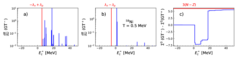
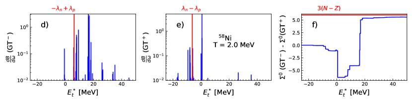
Figure 1: The temperature evolution of the Gamow-Teller strength distribution $dB/d\omega$ in ⁵⁸Ni with respect to the excitation energy $E^{*}_{t}$ of the parent nucleus in the (a),(d) GT^- and (b),(e) GT⁺ directions. Results are shown for temperatures (a)–(c) $T=0.5$ MeV and (d)–(f) $T=2.0$ MeV. The threshold between positive and negative energy transitions ($E^{*}_{t}=\pm(\lambda_{n}-\lambda_{p})$ for GT^±) is plotted with the red vertical line. (c),(f) the difference between zeroth moments $\Sigma^{0}(\text{GT}^{-})-\Sigma^{0}(\text{GT}^{+})$, with the red horizontal line denoting the result of the Ikeda sum rule $3(N-Z)$. Calculations are performed with the FT-HBCS+FT-PNRQRPA model using the D3C^∗ interaction.

IV.2 Sum rule with the relativistic FT-PNQRPA

The relativistic FT-PNQRPA (FT-PNRQRPA) calculation is based on the relativistic mean field theory where pairing correlations are treated within the finite-temperature Hartree Bardeen-Cooper-Schrieffer (FT-HBCS) theory with a monopole pairing interaction Yüksel et al. (2020); Ravlić et al. (2020). For the mean field part of the Hamiltonian we employ the D3C^∗ relativistic EDF Marketin et al. (2007) and assume spherical symmetry. The FT-PNRQRPA eigenvalue problem is derived from Eq. (4) by expanding the density response $\delta\tilde{\mathcal{R}}$ in the configuration space of the (quasi)proton-(quasi)neutron basis. For a detailed description of the method, check Refs. Sommermann (1983); Yüksel et al. (2017, 2020); Ravlić et al. (2021b). From the FT-PNRQRPA eigensolutions we compute the GT transition strengths according to Eq. (14) and construct the physical strength distribution from them by including the thermal prefactor,

$$\begin{split}\frac{dB}{d\omega}(\mathrm{GT}^{\pm})&=\frac{1}{1-e^{-\beta\omega}}\sum\limits_{k\pm>0}\left(|\langle[\Gamma^{k},\bm{\sigma}\tau_{\pm}]\rangle|^{2}\delta(\omega-\Omega_{k})\right.\\ &-\left.|\langle[\Gamma^{k},\bm{\sigma}\tau_{\mp}]\rangle|^{2}\delta(\omega+\Omega_{k})\right).\end{split}$$ (39)

To study the temperature evolution of the GT strength function and for the numerical check of the Ikeda sum rule, we select ⁵⁸Ni and perform calculations of the GT^± strength functions at temperatures $T=0.5$ and 2 MeV. For this calculation, the same numerical cut-offs are used as in Ref. Giraud et al. (2022). Namely, the nuclear ground state at finite temperature is obtained by solving the FT-HBCS equations in the spherical harmonic oscillator basis with $N_{\mathrm{osc}}=20$ oscillator shells. At the FT-PNRQRPA level, the maximal two-quasiparticle excitation energy is cut-off at 100 MeV, i.e., ${E_{\pi}+E_{\nu}<100~{}\mathrm{MeV}}$, and threshold for the product of FT-HBCS occupation amplitudes is set to $u_{(\pi,\nu)}v_{(\nu,\pi)}>0.01$. The monopole pairing strength for neutrons in ⁵⁸Ni is $G_{n}=24.3$ MeV/A, adjusted to reproduce the pairing gap calculated using the five-point formula Bender et al. (2000). Note that due to the shell closure at $Z=20$, no pairing occurs for proton states. Results are displayed in Fig. 1(a)–(c), for $T=0.5$ MeV and Fig. 1(d)–(f) for $T=2.0$ MeV. We plot the GT^± strength distributions as functions of the excitation energy with respect to the parent (i.e., the target) nucleus, $E^{*}_{t}=\omega\pm(\lambda_{n}-\lambda_{p})$ . The GT^- strength appears in Fig. 1(a),(d), the GT⁺ strength in Fig. 1(b),(e), and the difference between zeroth moments $\Sigma^{0}(\text{GT}^{-})-\Sigma^{0}(\text{GT}^{+})$ in Fig. 1(c),(f).

The main effect of finite temperature is the appearance of GT strength below the threshold, which is defined by $E^{*}_{t}=\pm(\lambda_{n}-\lambda_{p})$ for GT^± transitions. In the following, we denote such strength as de-excitations or simply, negative energy transitions. At $T=0.5$ MeV there is almost no contribution of the de-excitations. Overall, the strength function above threshold displays only moderate changes related to the reduction of pairing with increasing temperature. Since the FT-HBCS model is formulated within a grand canonical ensemble, a sharp vanishing of pairing gaps occurs at the critical temperature $T_{c}$ Goodman (1981). For ⁵⁸Ni pairing properties vanish at $T_{c}=0.74$ MeV. However, strength below the threshold increases with increasing temperature. This is a consequence of the thermal prefactor in Eq. (39) which allows for a larger number of transitions with excitation energies below the threshold to contribute to the strength function. At $T=2.0$ MeV the appearance of negative energy strength is clearly seen for both GT⁺ and GT^- transitions. Above the pairing collapse temperature, apart from inducing more transition strength below the threshold, temperature also modifies the strength function above the threshold due to the thermal unblocking, i.e., altering the occupation factors of quasiparticle levels. This effect allows for previously blocked transitions between fully occupied levels to occur.

In Fig. 1(c),(f), the difference between zeroth moments $\Sigma^{0}(\text{GT}^{-})-\Sigma^{0}(\text{GT}^{+})$ reproduces the Ikeda sum rule (red solid line) up to 93%. It is well known that for zero-temperature PNRQRPA based on relativistic interactions it is necessary to include the antiparticle-hole contribution to reproduce the sum rules Paar et al. (2003, 2004). In the present work we omit the antiparticle transitions for simplicity, and the small discrepancy in the sum rule is attributed to these missing contributions which, to a good approximation, can be neglected in charge-exchange calculations.

The above numerical example demonstrates the need for a consistent treatment of the FT-PN(R)QRPA strength function. To satisfy the Ikeda sum rule using the correct interpretation of the physical strength distribution, which includes the thermal prefactor, it is necessary to include the negative energy transitions.

IV.3 Sum rule with the finite amplitude method

To complement the calculations in Section IV.2, we now demonstrate the Ikeda sum rule for ⁵⁸Ni using the non-relativistic FT-PNQRPA and the charge-changing finite amplitude method (PNFAM) Mustonen et al. (2014). The FAM is an efficient means to solve the linear response equations while avoiding the expensive construction of the residual interaction matrix. It accomplishes this by computing the perturbation of the Hamiltonian directly with a finite difference,

$$\delta\widetilde{H}(\omega) =\frac{\partial H}{\partial R}\Bigg{\rvert}_{R=\widetilde{R}_{0}}\delta\widetilde{R}(\omega)$$ (40)

$$=\lim_{\eta\rightarrow 0}\frac{1}{\eta}\left[H[\widetilde{R}_{0}+\eta\delta\widetilde{R}(\omega)]-H[\widetilde{R}_{0}]\right]$$

$$=(\delta\widetilde{H}^{11},\delta\widetilde{H}^{20},\delta\widetilde{H}^{02},\delta\widetilde{H}^{\bar{11}})\,,$$

where $\widetilde{R}_{0}$ is the FT-HFB solution for the generalized density. In terms of the Hamiltonian perturbation, we can rearrange Eq. (1) to obtain the FT-FAM equations,

$$\left[\mathcal{E}-\omega M\right]\delta\widetilde{R}(\omega)=T\left[\delta\widetilde{H}(\omega)+\mathcal{F}(\omega)\right]\,,$$ (41)

which can be solved for the density response by iteration. From the FAM response we can then obtain the transition strength function through Eq. (15). In the charge-changing case, the perturbed Hamiltonian for Skryme functionals without proton-neutron mixing can be evaluated directly with the perturbed density, i.e., $\delta\widetilde{H}=H[\delta\widetilde{R}]$.

The Ikeda sum rule is computed from the residues of Eq. (15) for the Gamow-Teller external field operator. We obtain a sum of the residues via complex contour integration of the physical strength distribution,

$$\Sigma^{0}(\text{GT}^{\pm})=\frac{1}{2\pi i}\oint_{C}d\omega\ \frac{\widetilde{S}_{\mathrm{GT}^{\pm}}(\omega)}{1-e^{-\beta\omega}}\,,$$ (42)

where we take the contour $C$ to be a circle centered on the real axis.

The thermal prefactor appearing in Eq. (42), however, is difficult to treat with the complex contour integration method. We need to include strength from excitations at $\omega>0$ and de-excitations at $\omega<0$, but the thermal prefactor contains poles along the imaginary axis at $\omega=n(2\pi/\beta)i$ for $n=0,1,2,\ldots$ that should not be included in the contour integration. Naively, we might try to avoid these poles by using two contours. We can place one on either side of the imaginary axis and adjust the bounds so they come close to, but do not touch, the imaginary axis itself. In practice, however, if the boundary of a contour passes very near to one of these poles, the contour integration suffers numerical instabilities unless an unfeasibly dense discretization is used in the region near the pole.

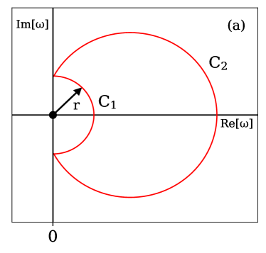
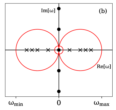
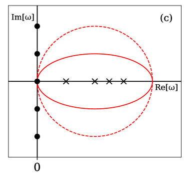
Figure 2: Schematic representations of (a) contours and pole at $\omega=0$ for the fractional residue proof (see main text), (b) all contours required for the finite-temperature sum rule, and (c) deforming the contour to avoid poles on the imaginary axis. Poles on the real and imaginary axes are black markers, with circles representing poles from the thermal prefactor and crosses poles from the FT-QRPA strength function.

Table 1: Contributions to the Ikeda sum rule in ⁵⁸Ni computed with the FT-PNFAM and the SKO’ interaction. Columns labeled % indicate ${(\Sigma^{0}(\mathrm{GT}^{-})-\Sigma^{0}(\mathrm{GT}^{+}))/3(N-Z)\times 100\%}$.

	$\omega<0$			$\omega>0$			Total
T[MeV]	$\Sigma^{0}(\mathrm{GT}^{+})$	$\Sigma^{0}(\mathrm{GT}^{-})$	%	$\Sigma^{0}(\mathrm{GT}^{+})$	$\Sigma^{0}(\mathrm{GT}^{-})$	%	$\Sigma^{0}(\mathrm{GT}^{+})$	$\Sigma^{0}(\mathrm{GT}^{-})$	%
0.0	$0.0$	$0.0$	$0.0$	$5.87592$	$11.86673$	$99.84677$	$5.87592$	$11.86673$	$99.84677$
0.5	$0.03442$	$0.00607$	$-0.47251$	$6.38447$	$12.41216$	$100.46141$	$6.41890$	$12.41823$	$99.98890$
1.0	$0.21849$	$0.08811$	$-2.17301$	$6.25650$	$12.38840$	$102.19831$	$6.47499$	$12.47651$	$100.02530$
1.5	$0.61711$	$0.19318$	$-7.06545$	$6.18013$	$12.60575$	$107.09364$	$6.79724$	$12.79893$	$100.02819$
2.0	$1.07395$	$0.45722$	$-10.27882$	$6.02681$	$12.64820$	$110.35647$	$7.10076$	$13.10542$	$100.07764$

Our solution to this problem is to use two contours on either side of the imaginary axis, but place them such that they pass through the pole at $\omega=0$. We find that, so long as no point on the discretized contour lies exactly on $\omega=0$, the integration yields a stable result with a reasonably dense grid. We can understand this behavior with the concept of fractional residues. One can prove that if $z_{0}$ is a simple pole of $g(z)$, and $C(r)$ is an arc of the circle defined by $\{r=\absolutevalue{z-z_{0}}\}$ subtended by an arc of angle $\alpha$, then Gamelin (2001),

$$\lim\limits_{r\rightarrow 0}\int_{C(r)}g(z)\,dz=\alpha i\,\text{Res}[g(z),z_{0}]\,.$$ (43)

Thus, if we take $C(r)$ to be $C_{1}$ in Fig. 2(a), in the limit that $r\rightarrow 0$ (and $C_{2}$ shifts such that $C_{1}$+$C_{2}$ remains a closed contour), we find that the contour integration yields half the usual residue, $\lim\limits_{r\rightarrow 0}\int_{C_{1}(r)+C_{2}}g(z)\,dz=\pi i\,\text{Res}[g(z),0]$. The inclusion of (a part of) the residue in the contour contributes to the stability of the numerical integration. Thus, to sum all the strength we can perform two types of integrations: one involving contours that intersect $\omega=0$, and one with a contour around just the pole at $\omega=0$ so that we can subtract (half) its contribution from the former results. The latter integration is numerically stable so long as the pole is centered in the contour, because the value of $\widetilde{S}_{F}(\omega)/(1-e^{-\beta\omega})$ will not vary much along the contour. Figure 2(b) exemplifies all the contours necessary for a complete calculation. This approach to the sum rule necessarily differs, for example, from the one described in Ref. Hinohara et al. (2013) because the thermal prefactor prohibits calculating the strength function near or along the imaginary axis.

While the contour integration method just described works well for high temperatures, for low temperatures the poles off the real axis can also get very close to the boundaries of large contours and induce instabilities in the integration. To address this issue, we deform the contour slightly into an ellipse such that the lowest pole on the imaginary axis is sufficiently far from the edge of the contour, as illustrated in Fig 2(c). We find that maintaining a distance of $2\pi/\beta$ is sufficient. For the smallest temperatures, this approach requires deforming the contour so much that it gets very close to the real axis everywhere, which is also undesirable. In these cases, however, the thermal prefactor is effectively a unit step function and de-excitations are negligible. We therefore neglect de-excitations and exclude the prefactor for temperatures at or below $1.0~{}\mathrm{GK}\approx 0.1~{}\mathrm{MeV}$.

Applying this procedure for summing the strength, we use the axially-deformed Skyrme PNFAM to calculate the Ikeda sum rule in ⁵⁸Ni for $T=0$–2 MeV. We use the Skyrme functional SKO’ fit for the global calculations of Refs. Mustonen and Engel (2016); Ney et al. (2020) with an effective axial vector coupling $g_{A}=1.0$. We included QRPA energies from $\omega=-50~{}\mathrm{MeV}$ to $+50~{}\mathrm{MeV}$, and 88 point Gauss-Legendre quadratures were performed for all contour integrations. Our results, which appear in Table 1, are within 0.1% of the exact sum rule for all temperatures studied. The very small deviation is likely attributed to a small amount of missing strength beyond the energy range considered and the buildup of small numerical errors. Although we do not gain information about the strength distribution from the contour integration, we can isolate the relative contributions from excitations ($\omega>0$) and de-excitations ($\omega<0$) to the sum rule. We see from Table 1 that de-excitations become increasingly important with temperature, accounting for more than 10% of the sum rule at a temperature of 2.0 MeV.

V Stellar electron capture rates

To exemplify how our presentation of the FT-QRPA impacts nuclear decays, we compute stellar EC rates. The stellar environment just prior to the supernova explosion (presupernova) is characterized by a high temperature $T$, and a product of baryon density $\rho$ and electron-to-baryon ratio $Y_{e}$ ($\rho Y_{e}$). Atoms are assumed to be fully ionized and the electron gas is described by a Fermi-Dirac distribution. Under the extreme presupernova conditions, nuclei can be found in highly-excited states. Decays from such states, characterized by negative $Q$-values, are known as de-excitations Dzhioev et al. (2010, 2019). Therefore, the FT-QRPA and its inclusion of transitions from thermally populated excited states is well suited to describe stellar weak-interaction rates. In this section, we investigate stellar EC rates using both relativistic and non-relativistic models from Section IV. Calculations are performed for ⁵⁸Ni and ⁷⁸Ni which are known to be of importance for the dynamics of CCSNe Sullivan et al. (2015); Suzuki et al. (2011).

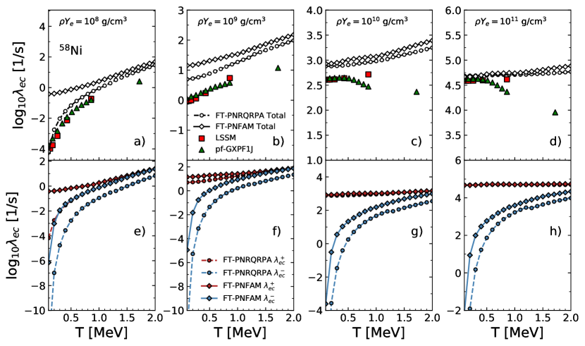
Figure 3: (a)–(d) the temperature dependence of the total electron capture (EC) rate $\lambda_{ec}$ in ⁵⁸Ni in the range $T=0$–$2$ MeV at stellar densities $\rho Y_{e}=10^{8}$–$10^{11}$ g/cm³. Results are calculated with the non-relativistic FT-PNFAM (diamonds) and relativistic FT-PNQRPA (circles), and compared with the large scale shell-model calculations (red squares) Langanke and Martínez-Pinedo (2000) and shell-model calculations based on the pf-GXPF1J interaction (green triangles) Suzuki et al. (2011); Mori et al. (2016). (e)–(h) contribution of the rate from excitations $\lambda_{ec}^{+}$ (red) and from de-excitations $\lambda_{ec}^{-}$ (blue) to the total EC rate as calculated with the FT-PNFAM (diamonds) and FT-PNRQRPA (circles).

Here we provide a brief outline of the EC rate calculation, with details appearing in Ref. Giraud et al. (2022). In this work we assume the allowed GT approximation, thus stellar EC rates can be written as

$$\lambda_{ec}=\frac{\text{ln}2}{\kappa}\frac{1}{Z}\sum\limits_{i,f}e^{-\beta\omega_{i}}|\langle f|\bm{\sigma}\tau_{+}|i\rangle|^{2}f(W_{0}^{i,f},\mu),$$ (44)

where $|i(f)\rangle$ are the exact initial (final) nuclear states with energy $\omega_{i(f)}$ and angular momenta $J_{i(f)}$, $\kappa=6147$ s is the decay constant, and $Z=\sum_{i}(2J_{i}+1)e^{-\beta\omega_{i}}$ is the partition function. The dimensionless phase space factor $f(W_{0}^{i,f},\mu)$ is an integral over electron energies $W=E_{e}/m_{e}c^{2}$, where $m_{e}$ is the electron mass. The energy $W_{0}^{(i,f)}$ is the maximum electron energy for the transition from $\ket{i}$ to $\ket{f}$ in the $\beta^{+}$ direction. The phase space integrand is folded with a Fermi-Dirac distribution of electrons, which depends on the electron chemical potential $\mu$ determined from the charge-neutrality condition for a given stellar density $\rho Y_{e}$ Giraud et al. (2022).

In the FT-QRPA, the EC rate can be expressed in terms of residues of the strength function

$$\lambda_{ec}=\frac{\text{ln}2}{\kappa}\sum\limits_{k\pm}\text{Res}\left[\frac{\tilde{S}_{\mathrm{GT}^{+}}(\omega)}{1-e^{-\beta\omega}}f(W_{0}[\omega]),\ \Omega_{k}\right],$$ (45)

where the summation is performed over FT-QRPA modes with both positive and negative eigenvalues and $W_{0}[\omega]$ is the threshold energy expressed in terms of the FT-QRPA perturbing energy $\omega$ Giraud et al. (2022). From the PNFAM, the sum of residues can be obtained via complex contour integration, while from the matrix theory the residues are computed from the FT-PNQRPA eigenvectors. In principle, at finite temperature the excitation energies can take values $-\infty<\omega<\infty$. However, the prefactor $(1-e^{-\beta\omega})^{-1}$ provides a cut-off for large negative energies, and the phase space integral provides a cut-off for large positive energies. To illustrate the contribution of de-excitations, we separate the rate into $\lambda_{ec}=\lambda^{+}_{ec}+\lambda^{-}_{ec}$, where $\lambda^{+}_{ec}=\lambda_{ec}\big{\lvert}_{\omega>0}$ is the rate from excitations and $\lambda^{-}_{ec}=\lambda_{ec}\big{\lvert}_{\omega<0}$ is the rate from de-excitations. The axial-vector coupling constant $g_{A}$ is quenched from the free nucleon value to $g_{A}=1.0$ in both calculations, consistent with previous works on EC Giraud et al. (2022); Ravlić et al. (2020); Niu et al. (2011); Paar et al. (2009).

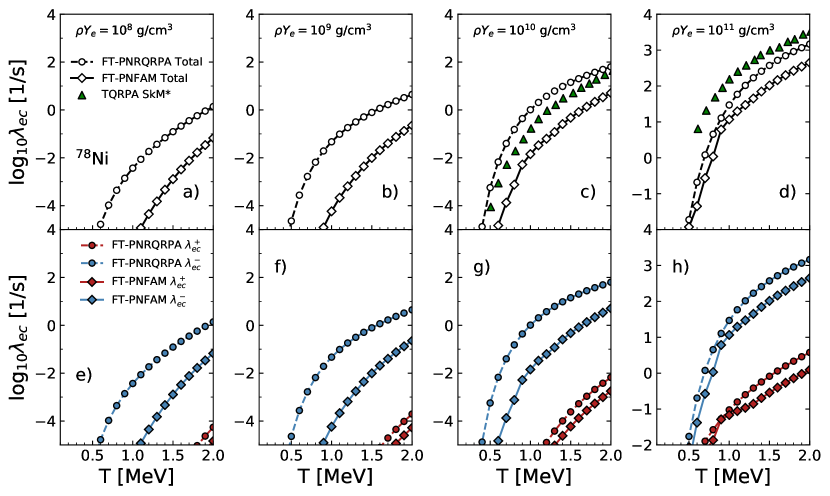
Figure 4: The same as in Fig. 3 but for ⁷⁸Ni. Results are compared with the TQRPA calculations based on the non-relativistic SkM^∗ interaction in Ref. Dzhioev et al. (2019) (green triangles).

In Fig. 3(a)–(d) we show the temperature dependence of the allowed $J^{\pi}=1^{+}$ EC rate $(\lambda_{ec}$) in ⁵⁸Ni at stellar densities in the range $\rho Y_{e}=10^{8}$–$10^{11}$ g/cm³. Results are displayed for both the relativistic FT-PNQRPA and non-relativistic FT-PNFAM calculations, and compared with the large scale shell-model calculations in Ref. Langanke and Martínez-Pinedo (2000) and the shell-model calculations based on the pf-GXPF1J interaction Suzuki et al. (2011); Mori et al. (2016). It is observed that EC rates in ⁵⁸Ni tend to increase with increasing temperature and increasing stellar density. The former is a consequence of the so-called thermal unblocking effect, where correlations due to finite temperature allow for previously blocked GT transitions (the contribution of de-excitations can be neglected for ⁵⁸Ni), while the latter stems from the fact that higher density implies higher electron chemical potential, thus allowing for more strength to contribute to the overall rate.

At the lower stellar densities of $10^{8}$–$10^{9}$ g/cm³ there are substantial differences in the total EC rate as calculated with the FT-PNFAM and FT-PNRQRPA. This is related to employing different model interactions. Namely, the FT-PNFAM employs the non-relativistic Skyrme SkO’ interaction and allows for axial deformations, while the relativistic FT-PNQRPA is based on the D3C^∗ interaction and is restricted to spherical configurations. This leads to systematic variance between two calculations since different effective interactions predict different quasiparticle bases. In particular, the FT-PNFAM calculation finds the potential energy surface of ⁵⁸Ni to be extremely shallow, with an oblate local minimum providing the lowest energy solution. Additionally, this axially-deformed ground state has a non-zero EC $Q$-value, explaining why the rate does not tend to zero at low temperatures and densities.

However, these differences become less important above the critical temperature for shape transition, where small deformation effects in ⁵⁸Ni get washed out Egido and Ring (1993a). Indeed, we observe differences between the model calculations decreasing with increasing temperature in Fig. 3. For higher stellar densities ($10^{10}$–$10^{11}$ g/cm³) the EC rates are almost independent of the particular details in the GT strength function, implying that only the overall GT strength matters Langanke et al. (2021); Giraud et al. (2022). Hence, the variance between both model calculations decreases with increasing $\rho Y_{e}$. A fair agreement of the total EC rate, as calculated with our FT-QRPA models, is obtained with respective shell-model calculations, although both FT-QRPA calculations tend to overestimate the shell-model EC rates.

In Fig. 3(e)–(h) the total EC rate in ⁵⁸Ni is decomposed into contributions from excitations ($\lambda_{ec}^{+}$) and de-excitations ($\lambda_{ec}^{-}$). It is observed that the rate due to de-excitations increases considerably with temperature. However, its overall impact on the total rate ($\lambda_{ec}$) is negligible up to $T=2$ MeV. A similar trend is confirmed for both model calculations in this work.

To observe how the contribution of de-excitations can lead to significant changes in the EC rates, in Fig. 4(a)–(d) we display the total EC rate in ⁷⁸Ni for stellar densities in the range $10^{8}$–$10^{11}$ g/cm³, with decomposition into the excitation and de-excitation rates in Fig. 4(e)–(h). Clearly, the contribution of de-excitations dominates the EC rates for all stellar densities, starting already at $T\approx 0.5$ MeV for both model calculations. It is larger than the respective excitation contribution by more than a few orders of magnitude. There is again variation between the FT-PNFAM and FT-PNRQRPA rates, but the trend is observed in both. Since ⁷⁸Ni is predicted as doubly-magic (and thus spherical) in both calculations, the variation is a consequence of different effective interactions. In Fig. 4(c)–(d) we have also displayed the data from Ref. Dzhioev et al. (2019) based on the TQRPA with the non-relativistic SkM^∗ interaction (green triangles). With the proper interpretation of the FT-QRPA strength function, as clarified in this work, we can reproduce the TQRPA rates with both the FT-PNRQRPA and FT-PNFAM. Otherwise, both FT-QRPA rates would considerably underestimate the TQRPA rates. Again, note that all three calculations use different effective interactions, thus agreement between the different models, FT-QRPA using either matrix FT-PNRQRPA or FT-PNFAM formulation, and the TQRPA is quite satisfying.

To explain why de-excitations dominate in ⁷⁸Ni but contribute much less in ⁵⁸Ni, we note that ⁵⁸Ni is located near the valley of stability, with a considerable amount of the GT⁺ strength (cf. Table 1). Therefore, the EC rates are going to have a significant contribution from the GT⁺ strength even at low temperatures. However, due to its neutron excess, GT⁺ strength in ⁷⁸Ni is substantially suppressed. On the other hand, because of its large GT^- strength, with increasing temperature the thermal prefactor in Eq. (45) allows for more strength to contribute to the total EC rate. This sudden jump in the de-excitation contribution at $\rho Y_{e}=10^{8}$ g/cm³ occurs around $T=0.5$ MeV, and at somewhat smaller temperatures at higher densities. Although with increasing stellar density the rate from excitations also increases, even at $\rho Y_{e}=10^{11}$ g/cm³ the de-excitation contribution for $T>0.5$ MeV is larger by a few orders of magnitude.

VI Conclusions

In this work, we presented a detailed investigation of the FT-QRPA derived in terms of thermal averages over the FT-HFB (or FT-HFBCS) statistical ensemble. We demonstrated connections between different formulations of the FT-QRPA linear response equations used in the literature and showed that all physical quantities are independent of the formulation used. Furthermore, we illustrated how the temperature-dependent metric formulation presents itself as the natural choice for the FT-QRPA equation because its properties mirror those of the zero-temperature QRPA. We then elucidated several properties of the FT-QRPA strength function, showing that the thermal prefactor and strength from both excitations and de-excitations are essential. We also located individual transitions in the FT-QRPA strength function, demonstrating that the strength at a given FT-QRPA energy approximates a thermal average over all transitions with a fixed transition energy.

To illustrate the correctness of our discussion, we employed two recently developed models in the charge-exchange channel: the non-relativistic, axially deformed FT-PNFAM based on the Skyrme EDFs and the relativistic, spherical FT-PNQRPA based on the meson-exchange D3C^∗ EDF. We verified analytically, and then numerically with both models for the case of ⁵⁸Ni, that the Ikeda sum rule is satisfied with the correct treatment of the FT-QRPA strength function. As a physical application, we then computed stellar EC rates for ^58,78Ni for a range of stellar densities and temperatures. Although de-excitations play almost no role in the EC rate for ⁵⁸Ni up to $T=2$ MeV, they dominate the EC rate in ⁷⁸Ni starting already from $T\approx 0.5$ MeV at $\rho Y_{e}=10^{8}$ g/cm³ because of its large negative $Q$-value. Only with the inclusion of de-excitations are we able to obtain reasonable agreement between our calculations and the EC rates based on the non-relativistic TQRPA calculations in Ref. Dzhioev et al. (2019). Similar trends are confirmed for both relativistic and non-relativistic FT-QRPA calculations in this work.

Recently, in Ref. Giraud et al. (2022) we have demonstrated that present models produce consistent results for EC rates of nuclei in the $N=50$ region, thus yielding small uncertainties for main CCSNe observables. This gives us confidence that the main correlations necessary for the description of EC rates are well enveloped, at least under extreme stellar conditions. Applying present models to other astrophysical scenarios, as well as to systematic calculation of EC rates across the nuclear chart, remain important tasks that should be pursued to further constrain astrophysical uncertainties.

Appendix A FT-QRPA proofs

In this section we enumerate several properties of the FT-QRPA matrix for the class of eigenvalue problems originating from Eq. (3),

$$(M\widetilde{\mathcal{S}}_{p})\ \delta\widetilde{R}_{p}^{k}=\Omega^{k}\ \delta\widetilde{R}_{p}^{k}\,.$$ (46)

Similar proofs for the zero-temperature RPA matrix are well-known, see for example Refs. Ring and Schuck (2004) and Ripka and Blaizot (1986). Here we extend these proofs to the $p$-dependent FT-QRPA eigenvalue problems and show they largely still apply in the same way as in the zero-temperature case, with a few caveats related to the temperature dependence. Moreover, we show that several key quantities are independent of $p$, demonstrating the equivalence of all formulations.

All of the proofs that follow require that the two-quasiparticle basis is constructed such that $E_{\alpha}>E_{\beta}$ and therefore $T$ is real and positive definite. Additionally, for the sake of simplicity we assume $\Omega^{k}\neq 0$.

Property 1.

Given the right eigenvalue problem in Eq. (46), the matrix $M\widetilde{\mathcal{S}}_{p}$ has a left eigenvector ${\delta\widetilde{L}_{p}=(\delta\widetilde{R}_{1-p}^{k})^{\dagger}M}$ with eigenvalue $\Omega^{k}_{(L)}=\Omega^{k*}$.

Proof.

By definition,

$$\delta\widetilde{L}_{p}^{k}(M\widetilde{\mathcal{S}}_{p})=\Omega^{k}_{(L)}\delta\widetilde{L}_{p}^{k}\,.$$ (47)

Using the claim for $\delta\widetilde{L}_{p}$ as an ansatz, the transpose of Eq. (47) states,

$$(M\widetilde{\mathcal{S}}_{p})^{T}(\delta\widetilde{L}_{p}^{k})^{T}=(MM\widetilde{\mathcal{S}}_{1-p}\ \delta\widetilde{R}_{1-p}^{k})^{*}=\Omega^{k*}(\delta\widetilde{L}_{p}^{k})^{T}\,.$$ (48)

The second equality follows from the properties $M^{2}=1$, and if $T>0$, then $T^{1-p}$ is real and $\widetilde{\mathcal{S}}_{p}^{\dagger}=\widetilde{\mathcal{S}}_{1-p}$. ∎

Property 2.

Eigenvectors of $M\widetilde{\mathcal{S}}_{p}$ are orthogonal if $\Omega^{k}\neq\Omega^{l*}$.

Proof.

For the non-hermitian eigenvalue problem, the norm is defined as the scalar product of left and right eigenvectors, and is independent of $p$,

$$\delta\widetilde{L}_{p}^{k}\delta\widetilde{R}_{p}^{l}=(\delta R^{k})^{\dagger}MT\ \delta R^{l}\,.$$ (49)

Now consider the left and right eigenvalue problems for any two solutions. Let us take the difference between

$$\delta\widetilde{L}_{p}^{l}\left[(M\widetilde{\mathcal{S}}_{p})\delta\widetilde{R}_{p}^{k}=\Omega^{k}\delta\widetilde{R}_{p}^{k}\right]\,,$$ (50)

and

$$\left[\delta\widetilde{L}_{p}^{l}(M\widetilde{\mathcal{S}}_{p})=\Omega^{l}_{(L)}\delta\widetilde{L}_{p}^{l}\right]\delta\widetilde{R}_{p}^{k}\,.$$ (51)

The $p$-dependence on the left-hand-side disappears, giving $(\delta R^{k})^{\dagger}\widetilde{\mathcal{S}}_{M}\delta R^{l}$ for both equations, which cancels after taking the difference. We are left with,

$$0=(\Omega^{k}-\Omega^{l*})(\delta R^{l})^{\dagger}MT\delta R^{k}$$ (52)

where we have used that $\Omega^{l}_{(L)}=\Omega^{l*}$ from Property 1. So long as $\Omega^{k}\neq\Omega^{l*}$, the eigenvectors are orthogonal. This result is independent of $p$. ∎

Corollary 2.1.

Eigenvectors belonging to complex eigenvalues have zero norm.

Proof.

If $\imaginary[\Omega^{k}]\neq 0$, then $\Omega^{k}-\Omega^{k*}\neq 0$, and Eq. (52) requires the norm to be zero. ∎

Property 3.

If the Hermitian matrix $\widetilde{\mathcal{S}}_{M}=T\mathcal{H}T+\mathcal{E}T$ has all positive eigenvalues, the eigenvalues of $M\widetilde{\mathcal{S}}_{p}$ are real and the sign of the eigenvalue matches the sign of the norm.

Proof.

Multiplying the right eigenvalue problem for $M\widetilde{\mathcal{S}}_{p}$ on the left by the corresponding left eigenvector leads to

$$(\delta R^{k})^{\dagger}\widetilde{\mathcal{S}}_{M}\delta R^{k} =\Omega^{k}(\delta R^{k})^{\dagger}MT\delta R^{k}$$ (53)

The right-hand side is the eigenvalue times the norm and the left-hand side is an expectation value of a Hermitian operator. To distinguish solutions of $\widetilde{\mathcal{S}}_{M}$ in the present context, we denote them with a subscript $(M)$. Using the completeness relation for the solutions of $\widetilde{\mathcal{S}}_{M}$ we can show,

$$(\delta R^{k})^{\dagger}\widetilde{\mathcal{S}}_{M}\delta R^{k}=\sum\limits_{n}\Omega^{n}_{(M)}\left\lvert(\delta R^{k})^{\dagger}\delta{R}_{(M)}^{n}\right\rvert^{2}\,.$$ (54)

Since $\widetilde{\mathcal{S}}_{M}$ is Hermitian, $\Omega_{(M)}^{n}$ are real and Eq. (54) proves the expectation value on the left-hand side is real. Inserting this result into Eq. (53), we can make the following conclusions:

1. If $\imaginary[\Omega^{k}]\neq 0$, by Corollary 2.1, the right-hand side of Eq. (53) vanishes, and therefore $\widetilde{\mathcal{S}}_{M}$ cannot have all positive eigenvalues.

2. If all of the eigenvalues of $\widetilde{\mathcal{S}}_{M}$ are positive, the eigenvalues of $M\widetilde{\mathcal{S}}_{p}$ are real and ${\text{sign}[\Omega^{k}]=\text{sign}[(\delta R^{k})^{\dagger}MT\delta R^{k}]}$.

∎

Property 4.

The right eigensolutions of $M\widetilde{\mathcal{S}}_{p}$ come in two sets. For every solution $\{\Omega^{k},\delta\widetilde{R}_{p}^{k}\}$, there is an orthogonal solution $\{-\Omega^{k*},\gamma\ \delta\widetilde{R}_{p}^{k*}\}$.

Proof.

The FT-QRPA matrix obeys the relation,

$$(M\widetilde{\mathcal{S}}_{p})^{*}=-\gamma\,(M\widetilde{\mathcal{S}}_{p})\,\gamma,\quad\gamma\equiv\begin{pmatrix}0&0&0&1\\ 0&0&1&0\\ 0&1&0&0\\ 1&0&0&0\end{pmatrix}\,.$$ (55)

From the complex conjugate eigenvalue problem, we can deduce,

$$(M\widetilde{\mathcal{S}}_{p}\delta\widetilde{R}_{p}^{k} =\Omega^{k}\delta\widetilde{R}_{p}^{k})^{*}$$ (56)

$$-\gamma M\widetilde{\mathcal{S}}_{p}\gamma\ \delta\widetilde{R}_{p}^{k*} =\Omega^{k*}\delta\widetilde{R}_{p}^{k*}$$

$$M\widetilde{\mathcal{S}}_{p}(\gamma\delta\widetilde{R}_{p}^{k*}) =-\Omega^{k*}(\gamma\delta\widetilde{R}_{p}^{k*})\,.$$

By Property 2, the eigenvectors $\gamma\delta\widetilde{R}_{p}^{k*}$ are orthogonal to $\delta\widetilde{R}_{p}^{k}$. We may call this result an upper-lower duality (by virtue of $\gamma$ swapping the upper and lower components of $\delta R^{k}$), while Property 1 defines a left-right duality. We can therefore summarize the FT-QRPA solutions accordingly:

	Upper	Lower
Right	$\{\Omega^{k},\ \delta\widetilde{R}_{p}^{k}\}$	$\{-\Omega^{k*},\ \gamma\delta\widetilde{R}_{p}^{k*}\}$
Left	$\{\Omega^{k*},\ (\delta\widetilde{R}_{1-p}^{k})^{\dagger}M\}$	$\{-\Omega^{k},\ (\delta\widetilde{R}^{k}_{1-p})^{T}\gamma M\}$

∎

Property 5.

If all the eigenvalues of $M\widetilde{\mathcal{S}}_{p}$ are real, the eigenvectors form a linearly independent complete set that obeys the closure relation in Eq. (60).

Proof.

The solutions are linearly independent if an only if

$$\sum\limits_{k}c^{k}\delta\widetilde{R}_{p}^{k}=0\,,$$ (57)

is satisfied by $c^{k}=0\ \ \forall\ \ k$. Multiplying by any left eigenvector, the orthogonality relation from Property 2 gives

$$\delta\widetilde{L}_{p}^{l}\sum\limits_{k}c^{k}\delta\widetilde{R}_{p}^{k}=c^{l}\ (\delta R^{l})^{\dagger}\,TM\,\delta R^{l}\,.$$ (58)

If all the eigenvalues are real, then all norms are non-zero, linear independence is satisfied, and the number of linearly independent vectors is equal to the dimension of $M\widetilde{\mathcal{S}}_{p}$, forming a complete set. Furthermore, the expression,

$$\sum\limits_{k}\delta\widetilde{R}_{p}^{k}\,\delta\widetilde{L}_{p}^{k}$$ (59)

applied to any vector in the complete set returns the same vector and is therefore equal to unity, proving the closure relation.

We can expand Eq. (59) to write the closure relation in terms of the upper and lower dual eigenvectors. If we take all positive eigenvalues to be in the set $\{\Omega^{k},\ \delta\widetilde{R}_{p}^{k}\}$, by Property 3 they have all have positive norms. Accordingly, the set $\{-\Omega^{k*},\ \gamma\,\delta\widetilde{R}_{p}^{k*}\}$ has all negative eigenvalues and negative norms. We can therefore normalize the upper and lower dual vectors to $+1$ and $-1$, respectively, and can write the closure relation as,

$$\sum\limits_{k>0}\delta\widetilde{R}_{p}^{k}\,\delta\widetilde{L}_{p}^{k}-(\gamma\delta\widetilde{R}_{p}^{k*})((\delta\widetilde{R}_{1-p}^{k})^{T}\gamma M)=1\,.$$ (60)

where the sum is over modes with positive norm. ∎

Property 6.

The $p$-dependent solutions of $M\widetilde{\mathcal{S}}_{p}$ can be used to calculate the same physical transition amplitude.

Proof.

The physical transition amplitude contains exactly one factor of $T$ as a result of taking the ensemble average. We can demonstrate this using the equations of motion of the FT-QRPA Sommermann (1983). For excitation operator,

$$\Gamma^{k\dagger}=\sum\limits_{\mu>\nu}P^{k}_{\mu\nu}b^{\dagger}_{\mu}b_{\nu}+X^{k}_{\mu\nu}b^{\dagger}_{\mu}b^{\dagger}_{\nu}-Y^{k}_{\mu\nu}b_{\nu}b_{\mu}-Q^{k}_{\mu\nu}b^{\dagger}_{\nu}b_{\mu}\,,$$ (61)

they read,

$$\left\langle\left[\delta\Gamma^{k},\left[H,\Gamma^{k\dagger}\right]\right]\right\rangle=\Omega^{k}\left\langle\left[\delta\Gamma^{k},\Gamma^{k\dagger}\right]\right\rangle\,.$$ (62)

This implies the amplitudes correspond to thermal averages as given in Eq. (13), so the ensemble averaged transition amplitudes are

$$\left\langle\left[\hat{F},\hat{\Gamma}^{k\dagger}\right]\right\rangle=\mathcal{F}^{\dagger}\,T\,\delta R^{k}\,.$$ (63)

Therefore, to get the physical transition amplitude from the eigenvectors of $M\widetilde{\mathcal{S}}_{p}$, we simply need to trace with the appropriate factor of $T$, i.e.,

$$\left\langle\left[\hat{F},\hat{\Gamma}^{k\dagger}\right]\right\rangle=(T^{1-p}\mathcal{F})^{\dagger}\delta\widetilde{R}_{p}^{k}\,.$$ (64)

∎

Appendix B Derivation of the Ikeda sum rule within the FT-H(F)B or FT-H(F)BCS

In the proton-neutron single-particle basis the external field operator can be written as

$$\hat{F}=\sum\limits_{pn}F_{pn}c_{p}^{\dagger}c_{n},$$ (65)

where $F_{pn}$ is the matrix element of the external field operator and $c^{\dagger}_{p(n)},c_{p(n)}$ proton (neutron) creation and annihilation operators respectively. To write the above expression in the quasiparticle basis we use the Bogoliubov transformation Ring and Schuck (2004)

$$c_{p}^{\dagger}=\sum\limits_{\pi}U_{p\pi}a_{\pi}+V^{*}_{p\pi}a_{\pi}^{\dagger},\quad c_{n}=\sum\limits_{\nu}U_{n\nu}^{*}a_{\nu}^{\dagger}+V_{n\nu}a_{\nu},$$ (66)

where $\pi$$(\nu)$ denotes the quasi-proton(neutron) states, $a^{\dagger}_{p(n)},a_{p(n)}$ are the corresponding quasiparticle operators and $U$, $V$ are the Bogoliubov matrices. The external field operator $\hat{F}$ in the quasiparticle basis has the form as in Eq. (35) with components

$$\begin{split}F^{11}_{\pi\nu}&=(U^{\dagger}FU)_{\pi\nu},\quad(F^{\dagger})^{11}_{\pi\nu}=(U^{T}FU^{*})_{\pi\nu},\\ F^{20}_{\pi\nu}&=(U^{\dagger}FV^{*})_{\pi\nu},\quad(F^{\dagger})^{20}_{\pi\nu}=(U^{T}F^{\dagger}V)_{\pi\nu},\\ F^{02}_{\pi\nu}&=(V^{T}FU)_{\pi\nu},\quad(F^{\dagger})^{02}_{\pi\nu}=(V^{\dagger}F^{\dagger}U^{*})_{\pi\nu},\\ F^{\bar{11}}_{\pi\nu}&=(V^{T}FV^{*})_{\pi\nu},\quad(F^{\dagger})^{\bar{11}}_{\pi\nu}=(V^{\dagger}F^{\dagger}V)_{\pi\nu}.\\ \end{split}$$ (67)

We can now evaluate the expression in Eq. (36) to get

$$\begin{split}\langle[\hat{F}^{\dagger},\hat{F}]\rangle&=\sum\limits_{pn}F_{pn}(F^{\dagger})_{pn}\left\{(UfU^{\dagger})_{nn}\left[(U^{*}U^{T})_{pp}+(VV^{\dagger})_{pp}\right]\right.\\ &-(U^{*}fU^{T})_{pp}\left[(UU^{\dagger})_{nn}+(V^{*}V^{T})_{nn}\right]\\ &-(V^{*}fV^{T})_{nn}\left[(U^{*}U^{T})_{pp}+(VV^{\dagger})_{pp}\right]\\ &+(VfV^{\dagger})_{pp}\left[(UU^{\dagger})_{nn}+(V^{*}V^{T})_{nn}\right]\\ &+\left.(U^{*}U^{T})_{pp}(V^{*}V^{T})_{nn}-(VV^{\dagger})_{pp}(UU^{\dagger})_{nn}\right\}.\end{split}$$ (68)

Using the unitarity of the Bogoliubov transformation Ring and Schuck (2004)

$$UU^{\dagger}+V^{*}V^{T}=1,\quad U^{*}U^{T}+VV^{\dagger}=1,$$ (69)

we can rewrite above expression as

$$\begin{split}\langle[\hat{F}^{\dagger},\hat{F}]\rangle&=\sum\limits_{pn}F_{pn}(F^{\dagger})_{pn}\left\{(UfU^{\dagger})_{nn}+[V^{*}(1-f)V^{T}]_{nn}\right.\\ &-\left.(U^{*}fU^{T})_{pp}-[V(1-f)V^{\dagger}]_{pp}\right\}\\ &=\sum\limits_{pn}F_{pn}(F^{\dagger})_{pn}\left\{n_{n}-n_{p}\right\},\end{split}$$ (70)

where $n_{n}=(UfU^{\dagger})_{nn}+[V^{*}(1-f)V^{T}]_{nn}$ and $n_{p}=(U^{*}fU^{T})_{pp}+[V(1-f)V^{\dagger}]_{pp}$ denote neutron and proton number of a given single-particle state. By inserting the GT operator as the external field

$$F_{pn}=\langle p||\bm{\sigma}\tau_{-}||n\rangle,\quad(F^{\dagger})_{pn}=\langle n||\bm{\sigma}\tau_{+}||p\rangle,$$ (71)

we get the well known result

$$\langle[\hat{F}^{\dagger},\hat{F}]\rangle=3(N-Z).$$ (72)

Same result can be reproduced within the H(F)-BCS formalism by replacing the Bogoliubov transformation with

$$c_{p}^{\dagger}=\delta_{p\pi}(u_{\pi}a_{\pi}^{\dagger}+v_{\pi}a_{\bar{\pi}}),\quad c_{n}=\delta_{n\nu}(u_{\nu}a_{\nu}+v_{\nu}a_{\bar{\nu}}^{\dagger}),$$ (73)

where $u,v$ are the H(F)-BCS amplitudes, and $\bar{\pi}$($\bar{\nu}$) denotes the time-reversed quasiparticle states Ring and Schuck (2004).

Appendix C Derivation of the Ikeda sum rule within the FT-PNQRPA

In this section we show that expression in Eq. (38) reduces to the well-known result of the Ikeda sum rule, $3(N-Z)$ Ikeda et al. (1963). We can rewrite Eq. (38) in matrix form as

$$\begin{split}&\Sigma^{0}(\hat{F})-\Sigma^{0}(\hat{F}^{\dagger})=\int\limits_{-\infty}^{\infty}d\omega\left[\frac{dB}{d\omega}(\hat{F})-\frac{dB}{d\omega}(\hat{F}^{\dagger})\right]\\ &=\sum\limits_{k\pm>0}\left(\frac{|\langle[\Gamma^{k},\hat{F}]\rangle|^{2}}{1-e^{-\beta\Omega_{k}}}-\frac{|\langle[\Gamma^{k},\hat{F}^{\dagger}]\rangle|^{2}}{1-e^{\beta\Omega_{k}}}\right)\\ &\qquad\qquad-\left(\frac{|\langle[\Gamma^{k},\hat{F}^{\dagger}]\rangle|^{2}}{1-e^{-\beta\Omega_{k}}}-\frac{|\langle[\Gamma^{k},\hat{F}]\rangle|^{2}}{1-e^{\beta\Omega_{k}}}\right)\\ &=\sum\limits_{k\pm>0}\left(|\langle[\Gamma^{k},\hat{F}]\rangle|^{2}-|\langle[\Gamma^{k},\hat{F}^{\dagger}]\rangle|^{2}\right)\\ &=\begin{pmatrix}\langle[\Gamma_{1},\hat{F}]\rangle^{*}\ldots\langle[\Gamma_{2N},\hat{F}]\rangle^{*}\langle[\Gamma_{1},\hat{F}^{\dagger}]\rangle\ldots\langle[\Gamma_{2N},\hat{F}^{\dagger}]\rangle\end{pmatrix}\\ &\times\begin{pmatrix}1&&&&&\\ &\ddots&&&&\\ &&1&&&\\ &&&-1&&\\ &&&&\ddots&\\ &&&&&-1\\ \end{pmatrix}\begin{pmatrix}\langle[\Gamma_{1},\hat{F}]\rangle\\ \vdots\\ \langle[\Gamma_{2N},\hat{F}]\rangle\\ \langle[\Gamma_{1},\hat{F}^{\dagger}]\rangle^{*}\\ \vdots\\ \langle[\Gamma_{2N},\hat{F}^{\dagger}]\rangle^{*}\\ \end{pmatrix},\end{split}$$ (74)

where $N$ is the number of (quasi)particle-(quasi)hole pairs, and the total dimension of the FT-PNQRPA matrix is $4N\times 4N$. The FT-PNQRPA equation can be written in the matrix form as already introduced in Sec. II

$$[\mathcal{E}+T\mathcal{H}]T\mathcal{X}=M{T}\mathcal{X}\mathcal{O},$$ (75)

where $\mathcal{X}$ is the matrix whose columns consist of the temperature-independent FT-PNQRPA eigenvectors

$$\mathcal{X}=\begin{pmatrix}P_{1}\ldots P_{2N}&Q_{1}^{*}\ldots Q_{2N}\\ X_{1}\ldots X_{2N}&Y_{1}^{*}\ldots Y_{2N}\\ Y_{1}\ldots Y_{2N}&X_{1}^{*}\ldots X_{2N}\\ Q_{1}\ldots Q_{2N}&P_{1}^{*}\ldots P_{2N}\\ \end{pmatrix},$$ (76)

while $\mathcal{O}=\text{diag}(\Omega_{1}\ldots\Omega_{N},-\Omega_{1},\ldots-\Omega_{N})$ contains the FT-PNQRPA eigenvalues (cf. Sec. II). Starting from the FT-PNQRPA phonon operator in Eq. (10) we can evaluate the required ensemble averages according to Eq. (14). It is straightforward to verify that

$$\begin{pmatrix}\langle[\Gamma_{1},\hat{F}]\rangle\\ \vdots\\ \langle[\Gamma_{2N},\hat{F}]\rangle\\ \langle[\Gamma_{1},\hat{F}^{\dagger}]\rangle^{*}\\ \vdots\\ \langle[\Gamma_{2N},\hat{F}^{\dagger}]\rangle^{*}\\ \end{pmatrix}=\mathcal{X}^{\dagger}T\mathcal{F}.$$ (77)

Using the normalization condition for the FT-PNQRPA eigenvectors

$$\mathcal{X}^{\dagger}TM\mathcal{X}=M,$$ (78)

Eq. (74) can be written as

$$\begin{split}&\Sigma^{0}(\hat{F})-\Sigma^{0}(\hat{F}^{\dagger})=\mathcal{F}^{\dagger}T\mathcal{X}M\mathcal{X}^{\dagger}T\mathcal{F}=\mathcal{F}^{\dagger}TM\mathcal{F}\\ &=F^{11}_{\pi\nu}(F^{\dagger})^{11}_{\pi\nu}(f_{\nu}-f_{\pi})+(1-f_{\nu}-f_{\pi})F^{20}_{\pi\nu}(F^{\dagger})^{20}_{\pi\nu}\\ &-(1-f_{\pi}-f_{\nu})F^{02}_{\pi\nu}(F^{\dagger})^{02}_{\pi\nu}-F^{\bar{11}}_{\pi\nu}(F^{\dagger})^{\bar{11}}_{\pi\nu}(f_{\nu}-f_{\pi}),\end{split}$$ (79)

which agrees with the expression for $\langle[\hat{F}^{\dagger},\hat{F}]\rangle$ of Eq. (36).

References

- Janka et al. (2007) H.-T. Janka, K. Langanke, A. Marek, G. Martínez-Pinedo, and B. Müller, Physics Reports 442, 38 (2007), the Hans Bethe Centennial Volume 1906-2006.
- Egido and Ring (1993a) J. L. Egido and P. Ring, Journal of Physics G: Nuclear and Particle Physics 19, 1 (1993a).
- Thielemann et al. (2017) F.-K. Thielemann, M. Eichler, I. Panov, and B. Wehmeyer, Annual Review of Nuclear and Particle Science 67, 253 (2017), https://doi.org/10.1146/annurev-nucl-101916-123246 .
- Kajino et al. (2019) T. Kajino, W. Aoki, A. Balantekin, R. Diehl, M. Famiano, and G. Mathews, Progress in Particle and Nuclear Physics 107, 109 (2019).
- Shlomo and Kolomietz (2004) S. Shlomo and V. M. Kolomietz, Reports on Progress in Physics 68, 1 (2004).
- Gross (1990) D. H. E. Gross, Reports on Progress in Physics 53, 605 (1990).
- Nikšić et al. (2011) T. Nikšić, D. Vretenar, and P. Ring, Progress in Particle and Nuclear Physics 66, 519 (2011).
- Schunck (2019) N. Schunck, ed., Energy Density Functional Methods for Atomic Nuclei, 2053-2563 (IOP Publishing, 2019).
- Roca-Maza and Paar (2018) X. Roca-Maza and N. Paar, Progress in Particle and Nuclear Physics 101, 96 (2018).
- Goodman (1981) A. L. Goodman, Nucl. Phys. A352, 30 (1981).
- Sano and Yamasaki (1963) M. Sano and S. Yamasaki, Progress of Theoretical Physics 29, 397 (1963), https://academic.oup.com/ptp/article-pdf/29/3/397/5367704/29-3-397.pdf .
- Goodman (1986) A. L. Goodman, Phys. Rev. C 34, 1942 (1986).
- Reiß et al. (1999) C. Reiß, M. Bender, and P.-G. Reinhard, The European Physical Journal A - Hadrons and Nuclei 6, 157 (1999).
- Martin et al. (2003) V. Martin, J. L. Egido, and L. M. Robledo, Phys. Rev. C 68, 034327 (2003).
- Niu et al. (2013) Y. F. Niu, Z. M. Niu, N. Paar, D. Vretenar, G. H. Wang, J. S. Bai, and J. Meng, Phys. Rev. C 88, 034308 (2013).
- TAKAHASHI and UMEZAWA (1996) Y. TAKAHASHI and H. UMEZAWA, International Journal of Modern Physics B 10, 1755 (1996), https://doi.org/10.1142/S0217979296000817 .
- Umezawa et al. (1982) H. Umezawa, H. Matsumoto, and M. Tachiki, Thermo field dynamics and condensed states (North-Holland, Netherlands, 1982).
- Paar et al. (2007) N. Paar, D. Vretenar, E. Khan, and G. Colò, Reports on Progress in Physics 70, 691 (2007).
- Ring et al. (1984) P. Ring, L. Robledo, J. Egido, and M. Faber, Nuclear Physics A 419, 261 (1984).
- Sommermann (1983) H. M. Sommermann, Ann. Phys. (N. Y.) 151, 163 (1983).
- Civitarese and DePaoli (1992) O. Civitarese and A. L. DePaoli, Zeitschrift für Physik A Hadrons and Nuclei 344, 243 (1992).
- Alasia and Civitarese (1990) F. Alasia and O. Civitarese, Phys. Rev. C 42, 1335 (1990).
- Dzhioev et al. (2016) A. A. Dzhioev, A. I. Vdovin, G. Martínez-Pinedo, J. Wambach, and C. Stoyanov, Phys. Rev. C 94, 015805 (2016).
- Dzhioev et al. (2015) A. A. Dzhioev, A. I. Vdovin, and J. Wambach, Phys. Rev. C 92, 045804 (2015).
- Dzhioev et al. (2020) A. A. Dzhioev, K. Langanke, G. Martínez-Pinedo, A. I. Vdovin, and C. Stoyanov, Phys. Rev. C 101, 025805 (2020).
- Dzhioev et al. (2010) A. A. Dzhioev, A. I. Vdovin, V. Y. Ponomarev, J. Wambach, K. Langanke, and G. Martínez-Pinedo, Phys. Rev. C 81, 015804 (2010).
- Dzhioev et al. (2009) A. A. Dzhioev, A. I. Vdovin, V. Y. Ponomarev, and J. Wambach, Physics of Atomic Nuclei 72, 1320 (2009).
- Dzhioev et al. (2019) A. A. Dzhioev, A. I. Vdovin, and C. Stoyanov, Phys. Rev. C 100, 025801 (2019).
- Dzhioev et al. (2008) A. A. Dzhioev, A. I. Vdovin, V. Y. Ponomarev, and J. Wambach, Bulletin of the Russian Academy of Sciences: Physics 72, 269 (2008).
- Barranco et al. (1985) M. Barranco, A. Polls, and J. Martorell, Nuclear Physics A 444, 445 (1985).
- Civitarese and Reboiro (2001) O. Civitarese and M. Reboiro, Phys. Rev. C 63, 034323 (2001).
- Civitarese and Ray (1999) O. Civitarese and A. Ray, Physica Scripta 59, 352 (1999).
- Civitarese et al. (2000) O. Civitarese, J. G. Hirsch, F. Montani, and M. Reboiro, Phys. Rev. C 62, 054318 (2000).
- Khan et al. (2004) E. Khan, N. Van Giai, and M. Grasso, Nuclear Physics A 731, 311 (2004).
- Minato and Hagino (2009) F. Minato and K. Hagino, Phys. Rev. C 80, 065808 (2009).
- Paar et al. (2009) N. Paar, G. Colò, E. Khan, and D. Vretenar, Phys. Rev. C 80, 055801 (2009).
- Yüksel et al. (2017) E. Yüksel, G. Colò, E. Khan, Y. F. Niu, and K. Bozkurt, Phys. Rev. C 96, 024303 (2017).
- Yüksel et al. (2019) E. Yüksel, G. Colò, E. Khan, and Y. F. Niu, The European Physical Journal A 55, 230 (2019).
- Niu et al. (2011) Y. F. Niu, N. Paar, D. Vretenar, and J. Meng, Phys. Rev. C 83, 045807 (2011).
- Niu et al. (2009) Y. Niu, N. Paar, D. Vretenar, and J. Meng, Physics Letters B 681, 315 (2009).
- Yüksel et al. (2020) E. Yüksel, N. Paar, G. Colò, E. Khan, and Y. F. Niu, Phys. Rev. C 101, 044305 (2020).
- Ravlić et al. (2021a) A. Ravlić, Y. F. Niu, T. Nikšić, N. Paar, and P. Ring, Phys. Rev. C 104, 064302 (2021a).
- Litvinova and Wibowo (2018) E. Litvinova and H. Wibowo, Phys. Rev. Lett. 121, 082501 (2018).
- Wibowo and Litvinova (2019) H. Wibowo and E. Litvinova, Phys. Rev. C 100, 024307 (2019).
- Litvinova and Wibowo (2019) E. Litvinova and H. Wibowo, The European Physical Journal A 55, 223 (2019).
- Litvinova and Robin (2021) E. Litvinova and C. Robin, Phys. Rev. C 103, 024326 (2021).
- Litvinova et al. (2020) E. Litvinova, C. Robin, and H. Wibowo, Physics Letters B 800, 135134 (2020).
- Chomaz et al. (1990) P. Chomaz, D. Vautherin, and N. Vinh Mau, Phys. Lett. B 242, 313 (1990).
- Sullivan et al. (2015) C. Sullivan, E. O’Connor, R. G. T. Zegers, T. Grubb, and S. M. Austin, The Astrophysical Journal 816, 44 (2015).
- Langanke et al. (2021) K. Langanke, G. Martínez-Pinedo, and R. G. T. Zegers, Reports on Progress in Physics 84, 066301 (2021).
- Giraud et al. (2022) S. Giraud, R. G. T. Zegers, B. A. Brown, J.-M. Gabler, J. Lesniak, J. Rebenstock, E. M. Ney, J. Engel, A. Ravlić, and N. Paar, Phys. Rev. C 105, 055801 (2022).
- Tanabe and Sugawara-Tanabe (1986) K. Tanabe and K. Sugawara-Tanabe, Physics Letters B 172, 129 (1986).
- Nakatsukasa et al. (2007) T. Nakatsukasa, T. Inakura, and K. Yabana, Phys. Rev. C 76, 024318 (2007).
- Avogadro and Nakatsukasa (2011) P. Avogadro and T. Nakatsukasa, Phys. Rev. C 84, 014314 (2011).
- Mustonen et al. (2014) M. T. Mustonen, T. Shafer, Z. Zenginerler, and J. Engel, Phys. Rev. C 90, 024308 (2014).
- Ripka and Blaizot (1986) G. Ripka and J.-P. Blaizot, Quantum theory of finite systems (The MIT Press, 1986).
- Vautherin et al. (1984) D. Vautherin, N. Mau, and N. Vinh Mau, Nucl. Phys. A 422, 140 (1984).
- Egido and Ring (1993b) J. L. Egido and P. Ring, J. Phys. G 19, 1 (1993b).
- Thouless (1961) D. J. Thouless, Nuclear Physics 22, 78 (1961).
- Ring and Schuck (2004) P. Ring and P. Schuck, The Nuclear Many-Body Problem (Springer, 2004).
- Ikeda et al. (1963) K. Ikeda, S. Fujii, and J. Fujita, Physics Letters 3, 271 (1963).
- Ravlić et al. (2020) A. Ravlić, E. Yüksel, Y. F. Niu, G. Colò, E. Khan, and N. Paar, Phys. Rev. C 102, 065804 (2020).
- Marketin et al. (2007) T. Marketin, D. Vretenar, and P. Ring, Phys. Rev. C 75, 024304 (2007).
- Yüksel et al. (2017) E. Yüksel, G. Colò, E. Khan, Y. F. Niu, and K. Bozkurt, Phys. Rev. C 96, 24303 (2017).
- Ravlić et al. (2021b) A. Ravlić, E. Yüksel, Y. F. Niu, and N. Paar, Phys. Rev. C 104, 054318 (2021b).
- Bender et al. (2000) M. Bender, K. Rutz, P.-G. Reinhard, and J. A. Maruhn, The European Physical Journal A 8, 59 (2000).
- Paar et al. (2003) N. Paar, P. Ring, T. Nikšić, and D. Vretenar, Phys. Rev. C 67, 034312 (2003).
- Paar et al. (2004) N. Paar, T. Nikšić, D. Vretenar, and P. Ring, Phys. Rev. C 69, 054303 (2004).
- Gamelin (2001) T. Gamelin, Complex Analysis (Springer, 2001) p. 209.
- Hinohara et al. (2013) N. Hinohara, M. Kortelainen, and W. Nazarewicz, Phys. Rev. C 87, 064309 (2013).
- Mustonen and Engel (2016) M. T. Mustonen and J. Engel, Phys. Rev. C 93, 014304 (2016).
- Ney et al. (2020) E. M. Ney, J. Engel, T. Li, and N. Schunck, Phys. Rev. C 102, 034326 (2020).
- Suzuki et al. (2011) T. Suzuki, M. Honma, H. Mao, T. Otsuka, and T. Kajino, Phys. Rev. C 83, 044619 (2011).
- Langanke and Martínez-Pinedo (2000) K. Langanke and G. Martínez-Pinedo, Nuclear Physics A 673, 481 (2000).
- Mori et al. (2016) K. Mori, M. A. Famiano, T. Kajino, T. Suzuki, J. Hidaka, M. Honma, K. Iwamoto, K. Nomoto, and T. Otsuka, The Astrophysical Journal 833, 179 (2016).