A Survey of CO, CO₂, and H₂O in Comets and Centaurs

Abstract

CO and CO₂ are the two dominant carbon-bearing molecules in comae and have major roles in driving activity. Their relative abundances also provide strong observational constraints to models of solar system formation and evolution but have never been studied together in a large sample of comets. We carefully compiled and analyzed published measurements of simultaneous CO and CO₂ production rates for 25 comets. Approximately half of the comae have substantially more CO₂ than CO, about a third are CO-dominated and about a tenth produce a comparable amount of both. There may be a heliocentric dependence to this ratio with CO dominating comae beyond 3.5 au. Eight out of nine of the Jupiter Family Comets in our study produce more CO₂ than CO. The six dynamically new comets produce more CO₂ relative to CO than the eight Oort Cloud comets that have made multiple passes through the inner solar system. This may be explained by long-term cosmic ray processing of a comet nucleus’s outer layers. We find (Q_CO/Q${}_{H_{2}O}$)_median = 3 $\pm$ 1% and (Q${}_{CO_{2}}$/Q${}_{H_{2}O}$)_median = 12 $\pm$ 2%. The inorganic volatile carbon budget was estimated to be (Q_CO+Q${}_{CO_{2}}$)/Q${}_{H_{2}O}$ $\sim$ 18% for most comets. Between 0.7 to 4.6 au, CO₂ outgassing appears to be more intimately tied to the water production in a way that the CO is not. The volatile carbon/oxygen ratio for 18 comets is C/O_median $\sim$ 13%, which is consistent with a comet formation environment that is well within the CO snow line.

1 Introduction

The physico-chemical conditions in the protosolar nebula varied with distance from the early Sun, which led to the freezing out of volatiles at different distances, and remnants from this early epoch are found in the ices of present day comets (Mumma & Charnley, 2011; Willacy et al., 2015; van Dishoeck & Bergin, 2020; Raymond & Morbidelli, 2020). Numerical models predict that most comets formed throughout a trans-Neptunian region (Nesvorný et al., 2017; Vokrouhlický et al., 2019) and that gravitational interaction with giant planets moved them into different orbits (Gomes et al., 2005; Tsiganis et al., 2005; Morbidelli et al., 2005; Walsh et al., 2011; Levison et al., 2011; Batygin, 2013; Brasser & Morbidelli, 2013). Comets are commonly sub-classified by their dynamical properties. For example, Jupiter Family comets (JFCs) have low-inclination orbits that mostly stay within Jupiter’s orbit and likely originated from the Kuiper Belt. Centaurs are low inclination comets in unstable orbits that are in transition between Kuiper Belt Objects (KBOs), also referred to as Trans-Neptunian Objects (TNOs), and JFCs (Dones et al., 2015a; Sarid et al., 2019). Oort Cloud comets (OCCs) have scattered inclinations with orbital distances extending as far as 10,000 - 50,000 au and rarely pass through the inner solar system. The Tisserand parameter with respect to Jupiter, T_J, is a numerical value calculated from orbital elements of a comet and Jupiter, and is often used in the classification schema. We adopt the identification of JFCs are comets with 2 <T_J <3, while OCCs and Halley type comets (HTCs) have T_J <2 (Levison, 1996). HTCs mostly orbit between Saturn and Neptune with higher inclination orbits, and some may originate from the Oort Cloud (Levison, 1996).

Measuring the relative abundances of key diagnostic cometary volatiles is a powerful constraint to solar system formation models (Lewis & Prinn, 1980; Pollack & Yung, 1980; Womack et al., 1992; Fegley, 1999; Lodders, 2003; A’Hearn et al., 2012; Guilbert-Lepoutre et al., 2015). The orbital families of comets and the chemical composition of their comae may be interdependent, and through observations we can test models of solar system formation (e.g., A’Hearn et al. (2012)). One critical pair of volatiles in comae is CO₂ and CO, and their abundance ratio is also useful for constraining physical models of comet nuclei as conveyed by outgassing behavior over different heliocentric distances (Prialnik et al., 2004; Belton & Melosh, 2009; Mousis et al., 2016; Sarid et al., 2019).

The most abundant parent volatile observed in comae is usually H₂O, followed by smaller contributions from CO₂, CO, and numerous relatively minor species (Bockelée-Morvan et al., 2004). Within heliocentric distance, R_Helio, of 2.5 au, water-ice sublimation proceeds efficiently and releases other volatiles, icy grains, and dust from the nucleus(Weaver, 1989; Prialnik et al., 2004; Meech & Svoren, 2004). Beyond $\sim$ 3 au, water-ice sublimation decreases substantially, and fewer comets show noticeable dust comae (Meech & Hainaut, 2001; Mazzotta Epifani et al., 2009; Ivanova et al., 2011; Sárneczky et al., 2016; Jewitt et al., 2017; Hui et al., 2019; Yang et al., 2021). Models of distant activity are generally based on a relatively unprocessed and volatile-rich nucleus and may include significant outgassing of other cosmogonically abundant volatiles in the nucleus, crystallization of amorphous water-ice process, sublimation of icy grains in the coma, jets, landslides, and even impacts (Womack et al., 2017). Because of outgassing variations with heliocentric distance, nucleus composition models must incorporate analysis of coma mixing ratios as a function of R_Helio (Huebner & Benkhoff, 1999). This paper focuses on CO and CO₂ measurements due to their relatively high abundance in comae and low sublimation temperatures, which are expected to contribute to cometary activity (Ootsubo et al., 2012; A’Hearn et al., 2012; Reach et al., 2013; Bauer et al., 2015). CO and CO₂ production rates are also useful for assessing the C/O ratio in comae, which is a key diagnostic of solar nebula chemistry in the comet-forming region (Öberg et al., 2011).

CO can be observed in comae from both ground- and space-based telescopes at a variety of its molecular transitions; however, due to severe telluric contamination and lack of a permanent dipole moment, CO₂ can only be observed directly from space. Indirect measurements of CO₂ emission are sometimes possible via spectroscopy of related CO Cameron bands and forbidden oxygen emission, but are difficult to carry out and not often derived with simultaneous CO production rates. Thus, the limiting volatile for this mixing ratio is CO₂, which has been detected or measured to significant limits in far fewer comets than CO. The largest single survey of simultaneous CO₂ and CO measurements thus far was made with the AKARI space telescope (Ootsubo et al., 2012). AKARI detected CO₂ in seventeen comets, but simultaneous detections or significant upper limits for CO were achieved in only eleven. The CO/CO₂ production rate ratios from the AKARI survey showed a great deal of variation among the comets with seven (64%) being CO₂-dominant. This was interpreted as possible evidence for a highly oxidized comet formation environment and/or that CO was exhausted near the surface of the comet nuclei (Ootsubo et al., 2012). By itself, the AKARI sample size of the CO/CO₂ mixing ratio in eleven comets was too small to test models of the predicted roles that comet families or heliocentric distance may have played.

In order to explore the CO/CO₂ mixing ratio in a much larger sample, as well as the parameters of comet families and heliocentric distances, we compiled a dataset of all contemporaneous CO and CO₂ measurements from the literature for 25 comets, and their water production rates when available. From this dataset we analyzed the production rate ratios for CO/CO₂, CO/H₂O, CO₂/H₂O, (CO+CO₂)/H₂O. We also present and discuss the C/O ratio, and the Q_CO/(surface area) and Q${}_{CO_{2}}$/(surface area) ratios derived using published diameters.

2 Methods and Analysis

We compiled all known published measurements of CO and CO₂ production rates in comets and Centaurs. The subset of objects for which both CO and CO₂ were detected or measured to a significant limit is given in Table 2.1. The vast majority of published production rates were calculated under the assumption that CO and CO₂ came from the nucleus, while some indicated that CO emission may also arise from an extended source and contribute another 10 - 50% to the overall CO coma (DiSanti et al., 1999; Brooke et al., 2003; Gunnarsson et al., 2008; Biver et al., 2018). For the one paper in this survey that did provide production rates for both nucleus and extended sources of CO (Combes et al., 1988), we used only the nucleus value for consistency with the other values. The CO₂ production rates we used were all assumed to be coming from the nucleus with no extended source contributions.

Half of the CO/CO₂ mixing ratios in this dataset were obtained using data obtained with the same technique (generally from space-borne infrared spectroscopy). The other half were compiled with different techniques and/or not truly simultaneous, but were close in time. Since a variety of ground- space-based techniques were used to collect these data, we briefly summarize them and explain how we handled issues that arose. For reference, the methods used for each comet are summarized in Table 2.1.

2.1 Overview of measurements techniques for CO and CO₂ measurements

Most of the Q_CO/Q${}_{CO_{2}}$ ratios were derived from observations of emission from the anti-symmetric stretch in the $\nu_{3}$ band of CO₂ at 4.26 $\mu$m and the first excited state to the vibrational ground state of CO at 4.67 $\mu$m (Crovisier et al., 1999a; Bockelée-Morvan et al., 2004). Spectroscopic techniques with AKARI, Vega, ISO, and Deep Impact/EPOXI space-based instruments provided simultaneous measurements of these bands in 15 comets (see Figure 1 and Table 5.1). When two aperture sizes were used (such as with the AKARI and Deep Impact instruments) we kept the data that were obtained with the larger aperture since it had the higher signal-to-noise ratio (Feaga et al., 2014). This may have introduced a small amount of emission from extended sources The production rates are 10-20% higher in the larger aperture sizes, but correcting for this is beyond the scope of this work and is probably within the uncertainties quoted for these comets. Wide bandpass filters spanning $\sim$ 4 - 5 $\mu$m were also used to measure these CO and CO₂ emission bands towards dozens of comets with the Spitzer (Reach et al., 2013) and NEOWISE space telescopes (Bauer et al., 2015). Unfortunately, this method collects photons from both species and cannot be used to derive individual measurements of each molecule (see Figure 1). It is also impossible to discern whether CO or CO₂ is observed from the filtered images without separate spectra of one of the volatiles. Except in rare cases (such as comets known to be either CO₂ or CO dominated, ie., 103P or 29P, respectively), the production rates in publications from the Spitzer and NEOWISE surveys are not good approximations for individual molecules, but instead serve as flags for targets of study and may be useful to track overall CO+CO₂ production. Due to the inability to determine a CO/CO₂ mixing ratio from these data alone, we did not include any production rates that were reported solely from the Spitzer or NEOWISE photometry techniques. We did, however, use these data when independent CO data were also obtained simultaneously, which permitted a CO₂ production rate to be inferred (see Section 2.2).

Because of a factor of $\sim$ 11.6 in fluorescence efficiencies (see Section 2.2), CO₂ will often have a higher line strength than CO at 4.5 $\mu$m wavelength region, even if the CO production rate is several times higher. An example of this can be seen in Figure 1, where the calculated CO production rate of Hale-Bopp was 5 times higher than that of CO₂, and yet the CO₂ line strength is noticeably taller in the spectrum. Moreover, the presence of a CO₂ line and absence of a CO emission line does not automatically convey that CO₂ is the dominant volatile, due to the significant difference in their fluorescence efficiencies. Numerous examples exist in the AKARI dataset (Ootsubo et al., 2012) where CO₂ was detected and CO was not, and yet CO’s production rate upper limit is higher than that derived from the CO₂ detection. Thus, caution should be used when interpreting which gas is likely dominating in 4.5 $\mu$m imaging or spectral data.

We included measurements of the CO J=2-1 rotational transition at 230 GHz that were obtained of C/2016 R2 using millimeter-wavelength spectroscopy with the Arizona Radio Observatory Submillimeter Telescope (Wierzchos & Womack, 2018). Due to its rotational symmetry, CO₂ does not have not any pure rotational transitions.

For several comets, we inferred the CO/CO₂ mixing ratio using indirect measurements. For example, CO₂ production rates relative to water can be inferred from optical spectra of forbidden oxygen lines when cometary and telluric emission is significantly separated by Doppler shift (Decock et al., 2013; McKay et al., 2016; Raghuram & Bhardwaj, 2014). These lines are formed when oxygen in an O-bearing molecule photodissociates and provides a green line at 5577Å and two red lines at 6300Å and 6364Å. Photochemical models predict that H₂O, CO₂, and CO in comae could all be the parents of the dissociation of oxygen, and that if the green to red doublet flux ratio (G/R) is larger than 0.1, then it is likely that either CO or CO₂ is the main parent and the percentage relative to H₂O can be estimated (Festou & Feldman, 1981; Cochran & Cochran, 2001). CO is not considered to be a large contributor to most cometary [OI] lines since the dissociation energy of CO to O(¹D) and O(¹S) is higher than the ionization energy (Raghuram et al., 2020). By itself, this method does not provide a way of discerning whether CO or CO₂ is present, and measurements from another technique are needed to see which molecule is dominant. For comets 46P and 21P, we used CO₂ production rate values that were derived from OI lines using the Harlan Smith Telescope and Subaru Telescope, respectively, while also using infrared spectroscopy with NASA IRTF iShell to establish the CO production rates (Roth et al., 2020; McKay et al., 2021; Shinnaka et al., 2020).

CO₂ and CO production rates were also derived from ultraviolet spectra of the CO Cameron and CO 4^th Positive bands. The Cameron bands ($a^{3}$ $\Pi\rightarrow$ $X^{1}$ $\Sigma^{+}$, central wavelength at 198.6 nm) are a spin forbidden transition of a CO molecule that is a dissociation product of CO₂, and thus can be used to infer CO₂ production rates (Raghuram & Bhardwaj, 2012). This technique works well for CO-depleted comets (comets 103P, C/1979 Y1 Bradfield, C/1989 X1 Austin, C/1990 K1 Levy), or comets which are observed with high enough spectral resolution (comets C/1996 B2 Hyakutake, 9P/Tempel, and 103P/ Hartley 2) (Bockelée-Morvan et al., 2004). Emission from the CO 4^th Positive bands ($A^{1}$ $\Pi\rightarrow$ $X^{1}$ $\Sigma^{+}$, central wavelength at 158.9 nm) can be modeled to provide CO production rates. The CO Cameron and 4^th Positive bands were also sometimes measured simultaneously to provide CO₂ and CO production rates, respectively, for comets C/1979 Y1 Bradfield, C/1989 X1 Austin, and C/1990 K1 Levy using the IUE SWP (Feldman et al., 1997) and for comet C/1996 B2 Hyakutake using the HST FOS (McPhate, 1999). Additional observations were used from the CO 4^th Positive bands obtained with the HST COS (for comet 103P) and ACS (for comet 9P) instruments (Weaver et al., 2011; Feldman et al., 2006).

Table 1: Overview of Simultaneous CO and CO₂ measurements in 25 comae

Instrument	Molecular transitions	Comets	References
AKARI IRC/NC	CO2 ($\nu_{3}$), CO v(1–0)	22P, 29P, 81P, 88P, 144P	1
”	”	C/2006 OF2, C/2006 Q1
”	”	C/2006 W3, C/2007 N3
”	”	C/2007 Q3, C/2008 Q3
Vega IKS	CO2 ($\nu_{3}$), CO v(1-0)	1P	2
ISO ISOPHOT-S	CO2 ($\nu_{3}$), CO v(1-0)	C/1995 O1	7
Deep Impact/EPOXI HRI	CO2 ($\nu_{3}$), CO v(1-0)	9P, 103P, C/2009 P1	4, 5, 9
Spitzer IRAC	CO2 ($\nu_{3}$), CO v(1-0)	C/2016 R2, C/2012 S1, 29P	8, 10, 14, 17, 18
ARO Submm Telescope	CO J=2-1	C/2016 R2	8, 14
Smith Optical Telescope	[OI] for CO2	46P	11
Subaru Telescope HDS	[OI] for CO2	21P	20
IRTF iShell	CO v(1-0)	21P, 46P	11, 19
IUE SWP	CO 4th Positive, CO Cameron	C/1979 Y1, C/1989 X1	13, 15
”	”	C/1990 K1
HST FOS	CO 4th Positive, CO Cameron	C/1996 B2	16
HST COS/ACS	CO 4th Positive	9P, 103P	3, 6
ROSETTA ROSINA	CO2, CO	67P	12

References. — 1: Ootsubo et al. (2012), 2: Combes et al. (1988), 3: Weaver et al. (2011), 4: A’Hearn et al. (2011), 5: Feaga et al. (2007), 6: Feldman et al. (2006), 7: Crovisier et al. (1999a), 8: McKay et al. (2019), 9: Feaga et al. (2014), 10: Lisse et al. (2013), 11: McKay et al. (2021), 12: Combi et al. (2020), 13: Feldman et al. (1997) 14: McKay, A. et al. (in prep), 15: Tozzi et al. (1998), 16: McPhate (1999), 17: Wierzchos (2019), 18: Meech et al. (2013), 19:Roth et al. (2020), 20: Shinnaka et al. (2020)

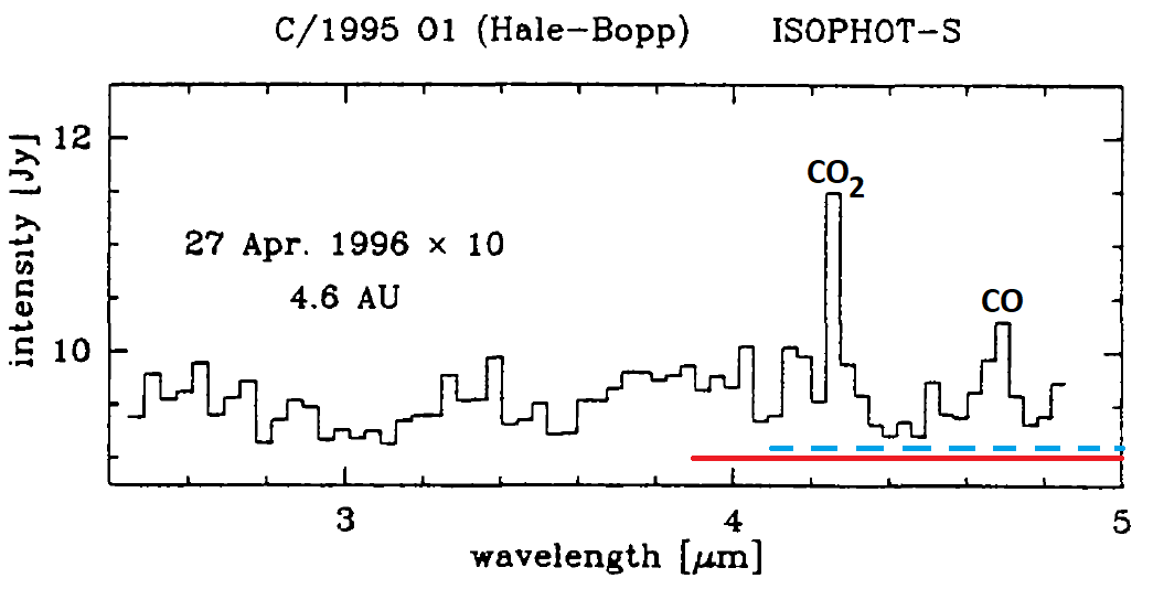
Figure 1: This figure shows the ambiguity of measuring CO₂ (4.26 $\mu$m) and CO (4.67 $\mu$m) production rates with broadband infrared imaging. The wavelength ranges for Spitzer IRAC channel 2 (red solid line) and for NEOWISE channel W2 (blue dashed line) are plotted on an infrared spectrum of comet C/1995 O1 Hale-Bopp obtained with the Infrared Space Observatory (adapted from the Figure 1 of Crovisier et al. (1999a)). Both CO and CO₂ emission bands fall within the channel bandpasses and cannot be distinguished without independent measurements of at least one of the volatiles. This figure also shows that the CO₂ emission line is $\sim$ 2x higher than CO’s, even though the CO production rate was five times greater, due to differences in fluorescence excitation rates.

We also used measurements obtained by spacecraft instruments for five comets. Vega 1’s IKS IR spectrometer provided CO and CO₂ data for gas production rates in 1P/Halley’s coma (Combes et al., 1988). Using the HRI-IR spectrometer, Deep Impact obtained measurements of CO₂ in 9P/Tempel 1 during its original mission (Feaga et al., 2007), and then of CO₂ in 103P/Hartley 2, and both CO and CO₂ in C/2009 P1 during its extended EPOXI mission (A’Hearn et al., 2011; Feaga et al., 2014). No detections were achieved for CO with the HRI-IR spectrometer for 9P/Tempel 1 and 103P/Hartley 2 (Feaga et al., 2007; A’Hearn et al., 2011), so we used measurements of the CO 4^th Positive bands that were obtained simultaneously with the CO₂ HRI-IR measurements to derive the CO/CO₂ mixing ratios (Feldman et al., 2006; Weaver et al., 2011). For 67P, we used analysis of data from the Rosetta ROSINA DFMS mass spectrometer for CO and CO₂ from Combi et al. (2020).

2.2 Inferring CO₂ from CO+CO₂ infrared photometry and independent CO measurements

We disambiguated the combined CO+CO₂ emission at $\sim$ 4.5 $\mu$m in Spitzer and NEOWISE infrared imaging data for three comets by using simultaneous independently measured CO emission. As an example, we explain the steps used with C/2016 R2 data. First, Spitzer data was used to calculate a gas production rate with the assumption that all the excess emission in the 4.5 $\mu$m range, after dust subtraction, came from CO. This is typically called the “CO production rate proxy”, Q${}_{CO_{proxy}}$ (Bauer et al., 2015). The CO production rate was also calculated using independent measurements, Q${}_{CO_{independent}}$ (in this case, the Arizona Radio Observatory 10-m Submillimeter Telescope) was subtracted from the Spitzer value, leaving a residual value, Q_residual:

$$Q_{CO_{residual}}=Q_{CO_{proxy}}-Q_{CO_{independent}}.$$ (1)

The residual CO proxy production rate was then converted to a CO₂ production rate following:

$$Q_{CO_{2}}=Q_{CO_{residual}}{{g_{CO}}\over{g_{CO_{2}}}},$$ (2)

where the fluorescence efficiencies at 1 au are $g_{CO}$ = 2.46 x 10^-4 sec^-1 and $g_{CO_{2}}$ = 2.86 x 10^-3 sec^-1 (Crovisier & Encrenaz, 1983).

At heliocentric distances less than $\sim$ 1.8 au, Spitzer CO+CO₂ observations can have significant dust contamination (Bauer et al., 2021). However, the data we used were obtained from comets well beyond that distance: C/2016 R2 was at 2.76 au and 4.73 au, C/2012 S1 was at 3.34 au, and 29P at 6.1 au. Thus, we do not think that there is any significant thermal dust signal contamination in the Spitzer data.

We provide additional details for inferring CO₂ from C/2012 S1 and 29P in Section 4.

2.3 When CO and CO₂ measurements are obtained with different techniques and/or are not simultaneous

CO₂, CO, and H₂O can rarely be detected simultaneously while using the same instrumentation, so some ratios are derived using different techniques and at slightly different times. We acknowledge that this mixing of techniques makes it difficult to quantify uncertainties of these derived ratios. Because modeling of CO, CO₂, and H₂O in comets is significantly hindered by lack of measurements we carefully included some measurements that were obtained with a different techniques. We alleviated this concern by analyzing case studies of when the individual volatiles were obtained by multiple techniques for a comet and checking for agreement in production rates that were obtained at overlapping times.

For example, with comet 9P, measurements of water production rates from the infrared are in excellent agreement with those derived from OH at 3080 Angstroms (Section 4.2). Similarly, the water production rates are in good agreement for those derived via IR and optical techniques for 46P (Section 4.6), and for those derived from IR, Radio and UV techniques for C/2016 R2 (Section 4.19). Regarding CO, the production rates for C/2016 R2 derived via IR and mm-wavelengths techniques, including with different telescopes and observing teams, agree very well (McKay et al., 2019). Similar excellent agreement was also found for CO in 29P with IR and mm-wavelength techniques (Senay & Jewitt, 1994; Paganini et al., 2013; Wierzchos & Womack, 2020; Bockelée-Morvan et al., 2022). CO₂ and H₂O production rates that were obtained for Hale-Bopp with a variety of different methods also showed good agreement (Weaver et al., 1997; Crovisier et al., 1999a; Biver et al., 2002). In particular, the CO₂ production rates for Hale-Bopp that were inferred from the ultraviolet CO Cameron bands are within $\sim$ 15% of the production rates derived from IR detections of CO₂ three days later (Weaver et al., 1997; Crovisier et al., 1999a). This is discussed in more detail in Section 4.12. This gave us confidence in combining production rates derived from different techniques. In Section 4 we provide more details of the comparisons for the multiple techniques observed for individual comets.

Since comets undergo heating that can significantly alter production rates and sometimes trigger outbursts, it is important to measure CO and CO₂ at the same time to ensure that the mixing ratio is not affected by changes in nucleus volatile production. There are many published measurements of CO and CO₂ for the same comet that were obtained weeks, months and sometimes years apart that we did not use to calculate a CO/CO₂ mixing ratio. There are not many instances where CO and CO₂ were measured at the same time or even approximately the same time, and all of the values are listed in Table 5.1, with the exception of 67P, which has a plethora of values of both volatiles from the Rosetta mission. The selected values of Q_CO and Q${}_{CO_{2}}$ for 67P in this study are representative of the comet’s behavior at the time and are not outliers. Unfortunately, there are not enough published data for all the other comets to establish long term production rates of CO2, especially in coordination with CO.

There are five comets for which measurements were not simultaneous, but were taken close enough in time to use: C/2016 R2, 9P, 21P, 46P, and 103P. CO and CO₂ data were obtained 11 hours apart for R2, 1.7 days apart for 9P, 1.1 days apart for 103P, 3 days apart for 46P, and 7 days apart for 21P. Extensive monitoring of these comets with all techniques indicated that there were no outbursts or significant variation in outgassing rates over the observed time periods, so we are confident about their mixing ratios being stable over these short time periods (Feaga et al., 2007; Feldman et al., 2006; A’Hearn et al., 2011; Weaver et al., 2011; McKay et al., 2021; Roth et al., 2020; Shinnaka et al., 2020).

2.4 Uncertainties of production rate ratios

Error bars for the production rate ratios in Figures 2, 3, 4, 5, 6, and 7 were calculated with the standard propagation of error using the production rate uncertainties. Unfortunately, publications do not always include these values. When production rate uncertainties were provided they are given in the tables, i.e., see Table 5.1, for 1P, C/1996 B2, C/2006 W3, C/2008 Q3, and C/2009 P1. These uncertainties ranged from 14% - 34% and the average was 20%. In order to estimate a reasonable uncertainty for the mixing ratios for the comets without published uncertainties, we assumed a 25% uncertainty for Q_CO and Q${}_{CO_{2}}$, which we do not include in the tables. Throughout Section 3 we also discuss how distantly active comets are more likely to have CO, CO₂, and/or H₂O detected, which might be a contributing factor to the lack of JFCs that we see beyond 3.5 au. This could contribute a bias in the results that is not accounted for in the numbers provided in the paper.

3 Results and Discussion

3.1 Aggregate findings: CO/CO₂

CO₂ and CO production rates were measured in the comae of 25 comets over the heliocentric distance range of 0.71 au to 6.18 au, with values ranging from Q${}_{CO_{2}}$ = (0.06 – 740) $\times$ 10²⁶ molecules sec^-1 (0.4 – 5,400 kg sec^-1) and Q_CO = (0.2 – 3,000) $\times$ 10²⁶ molecules sec^-1 (1 – 14,000 kg sec^-1) (see Table 5.1). The production rate ratios Q_CO/Q${}_{CO_{2}}$ are plotted against heliocentric distance in Figure 2. In order to facilitate comparison, we identified which volatile was dominant by marking these divisions in Figure 2, Figure 3, and Figure 4 using these dividing lines:

• Q_CO/Q${}_{CO_{2}}$ $\geq$ 4/3 (CO-dominant)

• 2/3 $<$ Q_CO/Q${}_{CO_{2}}<$ 4/3 (CO and CO₂ comparable)

• Q_CO/Q${}_{CO_{2}}$ $\leq$ 2/3 (CO₂-dominant)

These limits serve as a guide to help explore the volatile dominance shown by each comet. Upper limits to the production rate ratios were only included when they were less than or equal to 2/3. Only one lower limit was used (for Centaur 29P) where CO was detected and only a significant limit was set for CO₂ emission. As Figure 2 shows, the ratios vary significantly from Q_CO/Q${}_{CO_{2}}$ $\sim$ 0.01 for 103P/Hartley 2 at 1 au to Q_CO/Q${}_{CO_{2}}$ $>$ 98 for 29P at 6 au.

Using the above divisions and looking at all objects as an aggregate, thirteen comets (52%) fall in the CO₂-dominant category, nine (36%) are CO-dominant, and three (12%) have comparable amounts of CO and CO₂ in their coma (see Table 2). However, a closer look indicates that the mixing ratio may follow a trend with heliocentric distance, and there may be differences between comet families. We investigate these possibilities in the following sections.

3.2 Taxonomical families compared against CO/CO₂

A comet’s family assignment is typically made based on its current orbital parameters and deduced formation history (see Section 1). Comae compositional variations may be due to differences in formation scenarios and/or physical processing histories of comet nuclei after formation (Tsiganis et al., 2005; O’Brien et al., 2006; Mandt et al., 2015; Mumma et al., 2003; Mumma & Charnley, 2011). In this section we examine whether there are measurable differences between Q_CO/Q${}_{CO_{2}}$ ratios among the family groups of OCCs and JFCs. In Table 2 each cometary family is quantified based on their CO/CO₂ ratios.

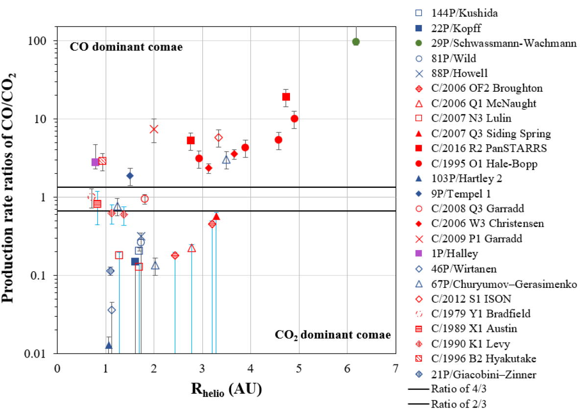
Figure 2: Q_CO/Q${}_{CO_{2}}$ production rate ratios are plotted vs. heliocentric distance for 25 comets. The objects are identified by name and are color coded to indicate family or class (red = Oort Cloud, blue = JFC, purple = Halley Type, green = Centaur). Two horizontal lines are drawn for values at $\pm$ 33% of 1, and comets within these two lines are considered to have comparable values of CO and CO₂ in their coma. Comae with Q_CO/Q${}_{CO_{2}}$ $\geq$ 4/3 are considered to be CO-dominant and those with Q_CO/Q${}_{CO_{2}}$ $\leq$ 2/3 are CO₂-dominant. Comets that are dynamically new are denoted with blue error error bars. Eight out of the nine JFCs are CO₂-dominated. The fourteen OCCs at first appear evenly distributed across the three categories, but including dynamical age divides them into two groups (see Figure 4). The aggregate data are consistent with CO becoming increasingly dominant in most comae beyond 3.5 au, possibly because CO requires a lower sublimation temperature than CO2. However, CO is not necessarily expected to dominate at large distances based on volatility effects alone. Since CO ice sublimates more efficiently than CO2 at large heliocentric distances, it could also be expected that CO should have been exhausted from at least the top layers of OCC nuclei long ago. Even so, mass loss of material during the perihelion passage might open deeper layers, which may be associated with the very high gas and dust production rates typical for many OCCs near perihelion.

As Figure 2 shows, eight of the nine JFCs fall in the CO₂-dominant category. 9P is the only JFC that has a CO-dominant coma, with Q_CO/Q${}_{CO_{2}}$ $\sim$ 2, as previously noted by A’Hearn et al. (2012). Given that most JFCs are thought to originate from Centaurs, it would be useful to see whether the CO/CO₂ mixing ratio changes as a comet moves from the Centaur to JFC region. The lone Centaur with a CO/CO₂ ratio, 29P, is CO-dominant, while most of the JFCs are CO₂-dominant; however, since 29P is at $\sim$ 6 au, it is subjected to much less heating than the JFCs, most of which were observed within $\sim$ 2.5 au, so 29P’s high CO abundance may be a solar heating effect. In contrast, the fourteen OCCs are more evenly distributed across the three categories with 36% of the OCCs (red) are CO₂-dominant, 43% are CO-dominant, and $\sim$ 21% have comparable amounts in their coma. Thus, looking at all the measurements combined, it seems as though JFCs might be more dominated by CO₂ than OCCs. However, there may be a selection effect at work. All of the JFCs were observed within 3.5 au, while the OCCs ratios were obtained across a larger range of heliocentric distances. The lack of data for JFCs beyond 3.5 au may be at least partly due to the fact that JFC nuclei tend to be smaller than those of OCCs. Smaller comets are generally less active at larger heliocentric distances and also fainter. Thus, the values at large heliocentric distances may not be typical of all distant comets (for example, consider the larger nuclei of Hale-Bopp and 29P at 6 au), and additional measurements of comets, especially JFCs, beyond 4 au are needed to better constrain cometary models.

Before exploring this difference in CO/CO₂ mixing ratios between JFCs and OCCs further for possible formation or physical processing causes, we search for possible solar heating effects since we have data ranging from 1 to 6 au.

Table 2: Overview of Comet Families in CO/CO₂ Survey

Family Class	CO2	CO	CO and CO2	Total
	Dominant	Dominant	Comparable
JFC	8	1	-	9
OCC	5	6	3	14
HTC	-	1	-	1
Centaur	-	1	-	1
Total	13	9	3	25

3.3 CO/CO₂ and heliocentric dependence or true anomaly

The aggregate data are consistent with an increasing CO/CO₂ production rate ratio with increasing distance from the Sun. In addition, all comae beyond $\sim$ 3.5 au are dominated by CO (see Figure 2). Although there are not many distantly active comets in this sample, they are all consistent with preferential release of CO over CO₂ from the nucleus. Coma abundances at large heliocentric distances may be a poor reflection of nucleus abundances, and instead, measurements of comets closer to the Sun might be a better indicator of nuclear abundances. Nonetheless, the larger heliocentric distance data are included to test models of the behavior of the release of volatiles from the nucleus as a function of heliocentric distance (Huebner & Benkhoff, 1999). Although we know that water-ice, the dominant volatile component in most comets, does not sublimate very efficiently at large distances, the outgassing of CO and CO₂ at large distances is not as well understood. The CO-dominance observed in comae beyond 3.5 au may be due to a few comets which have higher amounts of CO and are intrinsically more productive. This could also be caused by a heating effect on the nucleus and preferential release of volatiles for all comets. There are not many measurements of CO and CO₂ in JFCs observed beyond 3 au and so we cannot rule out a selection effect. More simultaneous measurements of CO and CO₂ production rates are needed in JFCs beyond 3 au to provide strong observational constraints.

Another way to explore possible heating effects is to examine the mixing ratio as a function of true anomaly, which is the angle between the periapsis and observed position relative to the Sun, and is often used to look for changes in a comet’s behavior as it goes through perihelion passage. In Figure 3 we do not see a significant difference between the CO/CO₂ mixing ratio in pre- and post-perihelion of any comets either as an aggregate group, or based on dynamical classes. However, all comets observed beyond $\pm$ 120 degrees are CO-dominant, which is consistent with also being beyond 3.5 au.

We have an opportunity to check for heliocentric dependence in this mixing ratio for four comets: C/2006 W3, C/1995 O1 Hale-Bopp, C/2016 R2, and 67P. Comets C/1995 O1 Hale-Bopp and C/2016 R2 were always CO-dominant and became slightly more CO-dominant after perihelion. C/2006 W3 produced slightly more CO than CO₂ when it was farther from the Sun pre-perihelion, but it was not measured post-perihelion. The Q_CO/Q${}_{CO_{2}}$ ratio of 67P varied in a complicated way during its perihelion passage. 67P was first measured as CO-dominated at $\sim$ 3.5 au pre-perihelion, then switched to CO₂-dominated from 3-2.5 au, and then produced approximately equal amounts of CO and CO₂ from 2 au to perihelion at 1.2 au. Thereafter, it switched to a CO₂-dominated coma, which it maintained for the most of the post-perihelion passage. Since most of the 67P measurements showed it to have far more CO₂ than CO, we put it in the CO₂ dominant category, although there are many many (20+) observations for the CO and CO₂ we only include three representative values for 67P in the figures. Clearly, the production of CO and CO₂ in 67P’s coma over time is complex and may be affected by the bi-lobed structure, which sometimes produced different amounts of volatiles (Combi et al., 2020) (see Section 4.7 for further discussion).

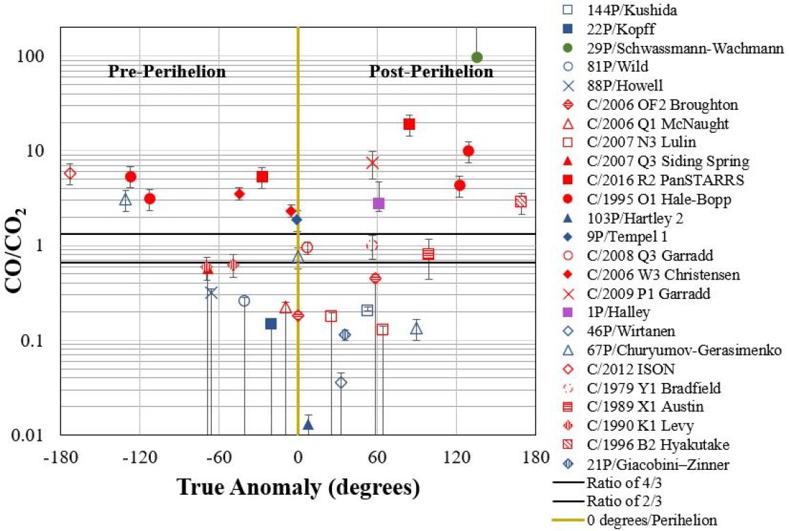
Figure 3: The CO/CO₂ production rate ratio is plotted against the true anomaly, which highlights the difference between pre- and post-perihelion values. Perihelion is at 0 degrees and is denoted with a yellow vertical line. Two horizontal lines are drawn within $\pm$ 33% of 1 and the color codes are the same as with Figure 2. The post-perihelion production rate ratios show a slight increase in CO post-perihelion for comets C/2016 R2 and C/1995 O1 Hale-Bopp. Comets with true anomalies greater than $\pm$ 120 degrees (both incoming and outgoing) are CO-dominant.

29P is a unique case since it is a Centaur and has a near-circular orbit at $\sim$ 6 au and is thus difficult to include in a heliocentric distance analysis. CO₂ was only measured once (as an upper limit) in 29P (and calculated indirectly twice, see Section 4.5, so it is not possible to study the mixing ratio’s change over time. However, the visible dust coma and CO production rate both show signs of a heliocentric dependence for the quiescent outgassing behavior, as well as a reported correlation of outbursts seen post-perihelion, see Wierzchos & Womack (2020) for details.

Due to the small number of comets observed, the significantly increased production of CO over CO₂ in distant comets can only be considered a preliminary result. If this holds for other comets, then it may be an important clue to the mechanical release of volatiles in distantly active comets and Centaurs when water-ice sublimation is less active. It is not clear how much CO-dominance beyond 3.5 au is due to a selection effect of comets with higher amounts of CO being intrinsically more productive and how much is due to a heating effect on the nucleus and the release of volatiles since CO requires a lower temperature to sublimate than CO₂.

Therefore, when considering comae beyond 3.5 au, and in the absence of information on both species, it may be appropriate to assume the dominant volatile is CO rather than CO₂, as originally noted in Figure 9 in Bauer et al. (2015). For example, when analyzing gaseous emission in NEOWISE and Spitzer CO+CO₂ images for comets beyond $\sim$ 3.5 au, when independent data is not available for either molecules, the default volatile proxy should be CO. In some cases, NEOWISE and Spitzer gas production rates values for comets beyond 3.5 au are provided in the literature as CO₂ values. Converting them to CO is straightforward and would increase the gas production rates by a factor of $\sim$ 11.6, the ratio of the fluorescence efficiencies (see Section 2.2). In addition, many comets within 3.5 au may produce a significant fraction of CO, so caution should be observed when relying on published CO₂ production rates from Spitzer and NEOWISE studies.

3.4 Dynamical Age (1/$a_{0}$) of Oort Cloud Comets

The number of perihelion passages a comet has made is directly related to the total heating its nucleus has experienced, which may in turn affect its coma composition. The inverse of the original semi-major axis, 1/$a_{0}$, is often used as a parameter for exploring solar heating in OCCs, since these comets have sustained stable orbits for a long period of time and are much farther from the Sun than JFCs or HTCs (A’Hearn et al., 1995). Furthermore, if we look at OCCs by their so-called dynamical age, we might expect that dynamically new (DN) comets would have experienced less processing from the Sun than dynamically older (DO) ones. Consequently, DN comet nuclei are typically assumed to have retained their primordial composition which should be evident in their comae near the Sun, including the CO/CO₂ mixing ratio.

Figure 4: Dynamical age, as probed with the inverse of the original semi-major axis, 1/a₀, is plotted for fourteen Oort Cloud comets within 3.5 au. We also plot the original semi-major axis, a₀, scale across the top axis. Dynamically new (DN) comets are often defined as those with 1/a₀ $<$ 10^-4 ${au}^{-1}$, which applies to the six left-most comets (C/2006 OF2 Broughton, C/2006 Q1 McNaught, C/2007 N3 Lulin, C/2007 Q3 Siding Springs, C/1989 X1 Austin, C/1990 K1 Levy). DN comets have the lowest CO/CO₂ ratios in this sample and a trend may be present with increasing CO produced with more thermal processing from the Sun (moving toward the right). OCCs on their first trip to the inner solar system produce more CO₂ than CO when within 3.5 au of the Sun, while those on their second or later trip tend to be CO-dominant. This is interesting, since CO is much more volatile than CO₂, and might be expected to have outgassed more than CO₂ over billions of years. Instead, this can be explained if CO ice is depleted from the outermost layer of the nucleus by galactic cosmic radiation during Oort Cloud storage, and then sublimates more readily after the outside cosmic-ray processed layer is eroded during its perihelion passage by the Sun, which exposes deeper layers where CO ice is still present (Maggiolo et al., 2020). As with previous figures, two horizontal lines are drawn within 33% of 1, and comets within these lines are considered to have comparable values of CO and CO₂ in their coma. DN comets are are highlighted by having blue error bars rather than black error bars.

In Figure 4 we plotted the CO/CO₂ production rate ratios of each OCC observed within 3.5 au as a function of 1/a₀. Within 3.5 au, water-ice sublimation proceeds efficiently and we can assume a quasi-steady-state coma abundance for CO and CO₂. We use 3.5 au as the cutoff rather than an even more conservative 2.5 au, because the identity of a CO-dominated or CO₂-dominated coma of these comets did not change between 2.5 and 3.5 au, and using 3.5 au provides more data points to probe whether CO or CO₂ was more dominant in the coma. For example, all of the CO/CO₂ ratios that we have for C/2006 OF2 shows that it had more CO₂ than CO in its coma, whether we use the measurements at 2.4 au or 3.2 au. We include only one data point for each comet and use the lowest heliocentric distance measurement available in order to minimize possible solar heating effects.

Table 3: Abundances Relative to Water for Comets under 2.5 au

Volatile/s	# JFCs	# OCCs	# HTCs	# Interstellar	Total # Comets	% of Water (Median)
CO	6	23	3	1	32	3 ± 1
CO2	14	8	1	-	23	12 ± 2
CO+CO2	9	8	1	-	18	18 ± 4

Interestingly, Figure 4 shows that comets on their first trip to the inner solar system produce more CO₂ than CO, while those on their second or later trips tend to produce more CO. This is the opposite of what models typically predict, which is that comets with the longest time in the Oort Cloud should have the more pristine composition. This result is consistent with what was found in a smaller study of only five comets (A’Hearn et al., 1995), which at the time was attributed to small-number statistics and/or by selection effects in the data set. Now with almost triple the number of comets in the 2012 study we see the same trend that DN comets produce more CO₂ relative to CO than the other Oort Cloud comets that have made multiple passes through the inner solar system.

This result may be explained by a model in which galactic cosmic ray impacts damaged ices in the outer layers of OCCs (while JFCs and Centaurs were relatively protected in the ecliptic). This led to a preferential loss of CO over CO₂ in these top layers down to several meters (due to CO’s much lower sublimation temperature and the modest energy increase from the cosmic rays), which then is observed in the low CO/CO₂ mixing ratios during the comets’ first approach to the Sun. This highly processed layer is significantly eroded and more well-preserved ices are exposed and outgas during subsequent perihelia (Gronoff et al., 2020; Maggiolo et al., 2020). Thus, the comae of DO comets are more pristine than those of DN comets. Figure 4 also shows that there may be a trend of increasing CO produced with more solar passages (increasing 1/a₀) for dynamically older comets, which should be confirmed with more measurements. Further efforts to confirm this observational result and to test models of comet nucleus processing from both solar heating and cosmic irradiation over very long periods are strongly encouraged.

One exception to the trend of increasing Q_CO/Q${}_{CO_{2}}$ with increasing 1/a₀ is C/1979 Y1, which is the dynamically oldest comet in this study and yet has comparable amounts of CO and CO₂, instead of producing far more CO. Including HTC 1P/Halley in Figure 4, would put it all the way to the right as the most solar radiation processed comet in the figure, just beyond C/1979 Y1, and it has a CO/CO₂ mixing ratio of $\sim$ 3. Interestingly, C/1979 Y1 may more accurately belong in the HTC category based on its orbital characteristics (Section 4). Thus, 1P’s CO/CO₂ mixing ratio more closely resembles that of the other DO OCCs than C/1979 Y1. Comets Y1 and 1P might be another part of the trend that link DO comets and HTCs, or that 1P and/or C/1979 Bradfield are outliers. Adding all of the available data (including the JFCs) to Figure 4 would introduce more CO₂-dominant comae to the far right side. It is interesting that the CO/CO₂ mixing ratios of the dynamically new OCCs are comparable to those of the highly-processed JFCs and yet are possibly explained by different types of processing - cosmic irradiation for the DN and solar irradiation for the JFCs.

Whether this result that DN comets produce more CO₂ than CO at perihelion holds for all Oort Cloud comets can be tested this year with the DN comet C/2017 K2 (PanSTARRS), which first became active at large distances. CO was detected in K2 at 6.7 au with Q_CO = 1.6 x 10²⁷ molecules/sec (Yang et al., 2021). K2 has 1/a₀ = 4.4x10^-5 (according to MPC) and thus would be located between C/2006 Q1 and C/1990 K1 on the figure. If K2’s nucleus has preferentially lost CO relative to CO₂ in its outer layers due to cosmic ray processing, then it is likely to have Q_CO/Q${}_{CO_{2}}$ <2/3 and will produce at least as much CO₂ as CO when it is near perihelion on Dec 19, 2022 at 1.8 au. Future measurements of both CO and CO₂ emission in C/2017 K2, and other DN comets, are needed to confirm the unexpected results in Figure 4 and cosmic ray processing model of Gronoff et al. (2020); Maggiolo et al. (2020).

Figure 5: CO/H₂O data from 45 comae. Comets from the previous figures are plotted using the same color scheme. Comets that did not have simultaneous CO and CO₂ detections are plotted with new colors: added OCCs are magenta, added JFCs are cyan, and one added interstellar comet is orange (2I/Borisov). The dashed horizontal line shows the median of all data (except Borisov) obtained within R${}_{Helio}<2.5$ au: (Q_CO/Q${}_{H_{2}O}$)_median = 3.3 $\pm$ 1.3%, with a higher Q_CO/Q${}_{H_{2}O}$ value for most OCCs compared with JFCs. This plot also shows how anomalous C/2016 R2’s composition was compared to all other comets and is consistent with a very distant formation region beyond the CO snow line, while most other comets have low CO/H₂O ratios consistent with formation within the CO snow line. Outside 2.5 au, the fractional abundance of CO to H₂O steadily increases, which is likely due to the decreased efficiency of water-ice sublimation at larger heliocentric distances. Overall, a two-slope fit to this data results in Q_CO/Q${}_{H_{2}O}$ $\sim$ R${}_{Helio}^{1.6}$ between 0.5 au to 2.5 au, and Q_CO/Q${}_{H_{2}O}$ $\sim$ R${}_{Helio}^{3.6}$ from 2.5 au to 4.6 au. The fits were calculated using detections only and did not include upper limits, nor were they weighted by uncertainties. Beyond 2.5 au, the slope for CO/H₂O is noticeably steeper than that for CO₂’s/H₂O (see Figure 6). Accounting for the upper limits would further increase the CO/H₂O slope for the large R_Helio comets, but also increase the scatter in the fit. At larger distances there are fewer measurements, and the fit from 2.5 au to 4.6 au should be considered with caution. The data are listed in Table 5.1 and Table 5.1.

3.5 CO/H₂O, CO₂/H₂O, (CO+CO₂)/H₂O, and C/O production rate ratios

We also used the compiled production rates to examine the relative amounts of CO and CO₂ with respect to H₂O and to explore the total carbon volatile budget in comae. CO, CO₂, and H₂O production rates are listed in Table 5.1 when all three volatiles were measured contemporaneously, and in Table 5.1 when either of the paired production rates of CO and H₂O, or CO₂ and H₂O, were obtained at the same time. Production rate ratios of Q_CO/Q${}_{H_{2}O}$ and Q${}_{CO_{2}}$/Q${}_{H_{2}O}$ as a function of heliocentric distance are plotted in Figure 5 and Figure 6, respectively. We also examined the combined CO and CO₂ production rates with respect to water in Figure 7 and the estimated volatile carbon/oxygen ratios in Figure 9. We discuss implications of these figures in this section.

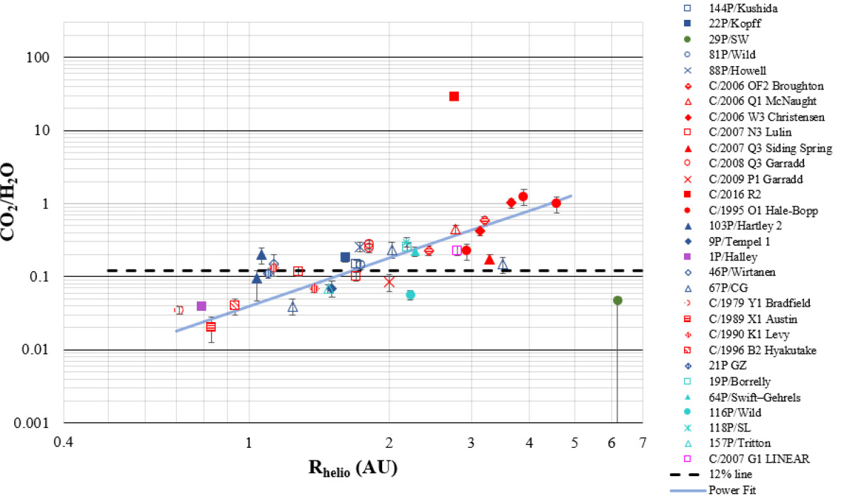
Figure 6: The fractional production rate of CO₂ to water is plotted against heliocentric distance and appears to follow a relationship of Q${}_{CO_{2}}$/Q${}_{H_{2}O}$ $\sim$ R${}_{Helio}^{2.2}$ from 0.71 to 4.58 au. In contrast to CO, the CO₂ to water ratio increases less steeply with heliocentric distance and shows a tighter correlation with heliocentric distance (compare to Figure 5). The dashed line indicates the median value of Q${}_{CO_{2}}$/Q${}_{H_{2}O}$ = 12% $\pm$ 2% for all comae below 2.5 au. The data are provided in Table 5.1 and Table 5.1.

Figure 5 shows the CO/H₂O production rate ratios plotted for 45 comets as a function of heliocentric distance and coded for orbital family. The CO/H₂O ratio for comae within 2.5 au (which includes 32 of the 45 comets) ranges from 0.3% to 26% with a median of 3.3 ± 1.3%. Within 2.5 au, the OCCs tend to have a higher CO/H₂O ratio than the JFCs, which may be in part due to different formation environments. This result is based on values from six JFCs, three HTCs, and 23 OCCs and should be confirmed with more observations. The median was calculated using detections in both Table 5.1 and Table 5.1, and no upper limits were used. If instead of a median, we calculate an average, we find CO/H₂O = 6.4 ± 1.3% within 2.5 au, which is consistent with what was reported for the average of 24 comets of 5.2 ± 1.3% in another study (Dello Russo et al., 2016).

The production rate ratio of Q_CO/Q${}_{H_{2}O}$ for all comae over the entire range of heliocentric distances observed (Figure 5) is noticeably steeper than that of Q${}_{CO_{2}}$/Q${}_{H_{2}O}$ (Figure 6). Moreover, the CO fractional abundance may exhibit a change in slope at $\sim$ 2.5 au, being flatter interior and steeper further out. To illustrate this point and for easier comparison with the CO₂ data, we calculated two slopes using a least squares fit, resulting in Q_CO/Q${}_{H_{2}O}$ $\sim$ R${}_{Helio}^{1.6}$ between 0.5 au to 2.5 au, and Q_CO/Q${}_{H_{2}O}$ $\sim$ R${}_{Helio}^{3.6}$ from 2.5 au to 4.6 au. The CO/H₂O data have a significant amount of scatter and we caution against over-interpreting these values, but it is worth noting that this possible change in slope for CO/H₂O at 2.5 au coincides with the distance within which the water ice sublimation starts to become less efficient. When looking at the fits to Figure 5 the large heliocentric measurements of comets are biased towards comets that are active and productive enough to be measured, and so tend to favor larger comets. Since the upper limits were not included in the fits to Figure 5 a possible bias might be introduced again against lower CO comets being included in the analysis. If upper limits were included, the slopes would be even steeper and the scatter would be increased.

The CO₂/H₂O production rate ratios were compiled for 23 coma measurements within 2.5 au, and they range from 2% to 30% with a median value of (Q${}_{CO_{2}}$/Q${}_{H_{2}O})_{median}$ = 12 ± 2%. For comparison, the median is $\sim$ 30% smaller than the 17% value derived by Ootsubo et al. (2012). We attribute this difference to our sample size being almost twice as large as the AKARI survey, and to the fact that most of these additional comets had much lower fractional CO₂/H₂O abundances.

In contrast to CO, the CO₂ to water ratio increases less steeply with heliocentric distance and shows a tighter correlation with water from 0.7 to 4.6 au with Q${}_{CO_{2}}$/Q_H2O $\sim$ R${}_{Helio}^{2.2}$ (again excluding C/2016 R2). This may mean that production of CO₂ is intimately tied to water production in a way that CO is not. In contrast, the CO production rate has a much stronger response to solar heating than CO₂, which is consistent with it being a much more volatile ice. Interestingly, despite apparent possible strong ties to water, the aggregate CO₂/H₂O data do not show evidence for a break in slope at $\sim$ 2.5 au where water-ice sublimation typically changes significantly for comets.

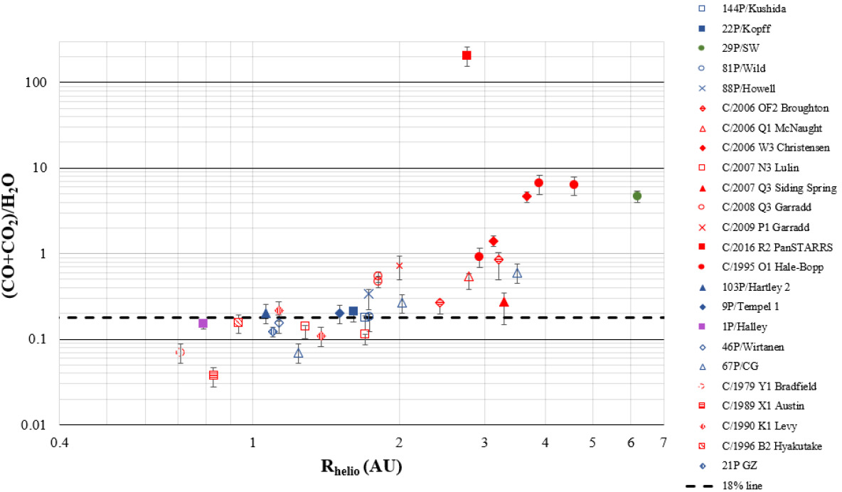
Figure 7: This figure plots the ratio of the total inorganic carbon-bearing volatile (as represented by CO and CO₂) to water production rates as a function of heliocentric distance. The same color conventions are used for the different comet families as the previous figures. The dashed line shows the location of the median production rate ratio of Q${}_{CO+CO_{2}}$/Q${}_{H_{2}O}$ = 18 $\pm$ 4% for all comets within 2.5 au.

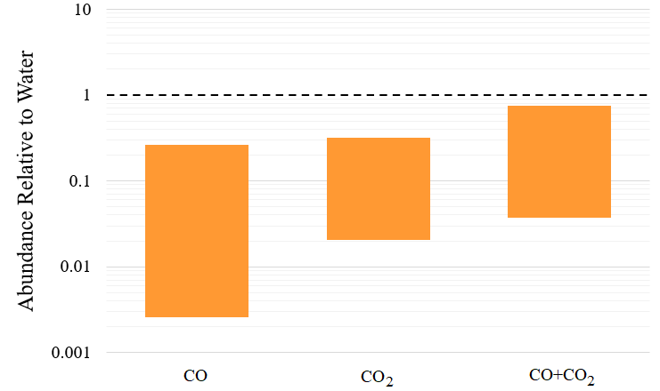
Figure 8: The ranges of fractional production rates of CO, CO₂, and CO+CO₂ with respect to water H₂O for comae within 2.5 au. The CO/H₂O ratio has a wider range than CO₂, which could be partly due to the fact that there are almost twice as many CO detections than CO₂. Although the (CO₂+CO)H₂O abundance ratio range in this figure is large, measurements for most comets fall within a much narrower range of 18% $\pm$ 4%, as shown in Figure 7.

We also examined the total CO+CO₂ production rates as a proxy for the total inorganic volatile carbon budget, since the vast majority of carbon will be found in these two volatiles (A’Hearn et al., 1995). Only 18 of the 25 comets that have CO and CO₂ production rates were observed below 2.5 au. We restricted our calculation to comets observed below 2.5 au, which should minimize possible bias introduced by differential outgassing of CO and CO₂ that we see farther out. The median production rate ratios of (Q_CO + Q${}_{CO_{2}}$)/Q${}_{H_{2}O}$ for all comets within 2.5 au is 18 ± 4%, although we point out that there is some substantial deviation from this value for a few comets (notably C/1989 X1 Austin with $\sim$ 3.7% and C/2009 P1 Garradd at $\sim$ 70%). However, most of the comets are consistent with the median value of 18%, which indicates that the total amounts of CO and CO₂ produced within 2.5 au may be conserved for most comets and is close to the $\sim$ 20% value proposed by A’Hearn et al. (2012); Lisse et al. (2021). Thus, the (Q_CO + Q${}_{CO_{2}}$)/Q${}_{H_{2}O}$ ratio for comets observed within 2.5 au could serve as a possible cosmogonic indicator providing insight on formation temperatures of the early solar system (Faggi et al., 2018; Lippi et al., 2020). This could support the theories that comets retain a strong amount of their natal composition. We are cautious because his study is based on a relatively small sample size, and more observations would be helpful to see how pervasive this is. We can also see that the CO+CO₂ seems to be well conserved in comets, and is indicative of comets forming in the same region. This is from the fact that when we look at comets observed within 2.5 au in Figure 7 (where there are about nine JFCs and eight OCCs), and most of the comets, regardless of their dynamical family, stay relatively level/flat along the median abundance ratio (i.e. no strong outliers like C/2016 R2) is suggestive that comets share a similar natal formation region.

Next, we consider the carbon/oxygen ratio tied up in gas comae as a probe of the cometary formation environment (c.f., Öberg et al. (2011); Eistrup et al. (2018)). We use CO, and CO₂ to represent carbon, since they are the largest carbon-contributors by far to the gas coma, and we use H₂O, CO, and CO₂ for the main contributors of oxygen (see Milam et al. (2006); Remijan et al. (2008); Dello Russo et al. (2016)). In Figure 9 we plot the carbon to oxygen ratio that we calculated using

$$C/O={{Q_{CO}+Q_{CO_{2}}}\over{Q_{CO}+2Q_{CO_{2}}+Q_{H_{2}O}}}$$ (3)

for all comets where all three species were detected at the same time (Table 5.1). A caveat is that the total cometary C/O ratio will also include the solid dust/grain component, but here we address only the volatile sources of carbon and oxygen as a probe of the gas and ice components.

The heating effects of solar radiation can be seen in Figure 9 where comets that are closer to the Sun produce significantly more water compared to carbon monoxide and carbon dioxide (resulting in a lower overall ratio). Within $\sim$ 2.5 au, where water sublimation is vigorous and individual comae probably achieved approximate compositional stability, we find C/O_average $\sim$ 15% and C/O_median $\sim$ 13%, which are similar to values found by Seligman et al. (2022) for a sample of solar system comets, and is consistent with these comets forming within the CO snow line (i.e., C/O $<$ 0.2) (Seligman et al., 2022). We see no distinction between the JFCs and OCCs with respect to C/O ratios within 2.5 au. This may be explained by models which predict that both Kuiper Belt and Oort Cloud reservoirs have similar origins and that they both formed within the region of the giant planets (i.e. 5-30 au), and were later moved to their present positions (see discussion by Dones et al. (2015b)). The low C/O gas-phase values are consistent with forming within the CO snow line Öberg et al. (2011)). Comets with higher values, such as C/2016 R2 with C/O $\sim$ 0.9, may have formed much farther out, even beyond the CO snow line. Caution should be used for high C/O values derived for comets beyond $\sim$ 3.5 au, such as C/2006 W3 Christensen, Hale-Bopp, and 29P, which are likely increased due to the lowered sublimation of water-ice at these distances and these values should not be used to constrain formation models.

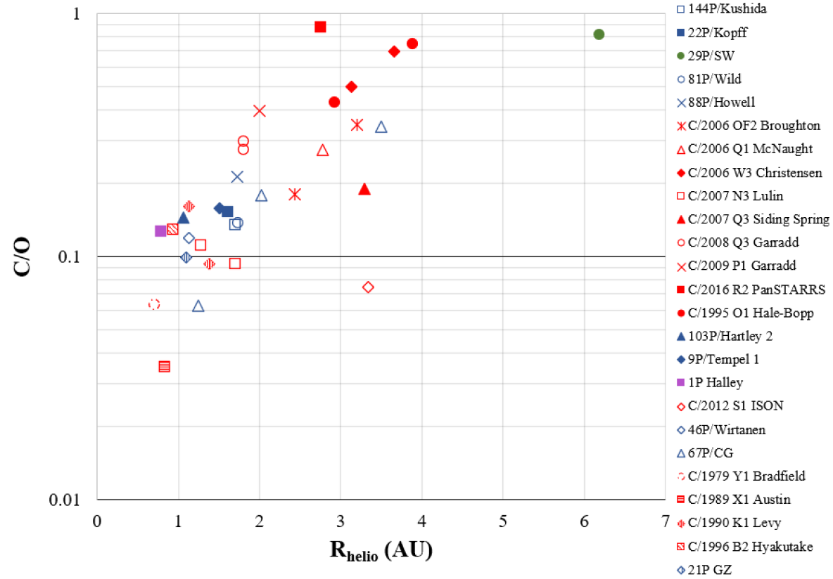
Figure 9: The carbon/oxygen ratio for the gaseous component (determined from CO, CO₂ and H₂O production rates) is plotted as a function over heliocentric distance. The same color convention is used for the different comet families as the previous figures. There is no discernible difference between the gaseous C/O ratios in JFCs and OCCs, which is consistent with the comet families forming in overlapping regions. The median C/O ratio in the gaseous component for comae within 2.5 au is $\sim$ 13%, and this low value is consistent with most comets forming within the CO snow line. C/2016 R2’s high value of C/O $\sim$ 0.9 is better fit by having formed much farther out, possibly beyond the CO snow line.

It is possible that water production rates may include substantial contributions from the sublimation of icy grains that have been dragged out from the nucleus, in addition to sublimating directly from water-ice on the nucleus (cf. A’Hearn et al. (2011); Sunshine & Feaga (2021)). For comets referred to as “hyperactive” (such as 21P, 41P, 45P, 46P, and 103P), the amount of water vapor may be substantial and even rival what is produced by direct sublimation of water ice from the nucleus and lead to what is reported as a lower CO/H₂O and CO₂/H₂O production rate ratio than what is actually coming from the comet. Thus for hyperactive comets we might be observing lower fractional abundances of CO and CO₂ due to the“over-production” of water. It is also possible that CO₂ ice grains can be ejected from CO which is more volatile. Other ejected ice grains that are from less volatile molecules (sublimate at higher temperatures) being released from gases that are more volatile (sublimate at lower temperatures) would increase the observed production rate of the volatile with the higher sublimation temperature. This would tend to increase the observed production rate of CO₂ over CO (Sunshine & Feaga, 2021). No attempt was made to separate those contributions in this analysis and we just use total water production rates. Caution is warranted for interpreting results for fractional water abundances in comets beyond $\sim$ 3 au since the coma abundances at larger heliocentric distances might be a poor reflection of nucleus abundances. The larger heliocentric observed comet data are provided to test models of their volatility as a function of heliocentric distance.

Opacity is another factor that could affect the production rates, especially for the inner coma and very productive comets. Most reported production rates were calculated assuming optically thin conditions and therefore had minimal-to-no corrections applied (Feldman et al., 2006; Feaga et al., 2007; Ootsubo et al., 2012; Feaga et al., 2014; McKay et al., 2015). In other cases, the optically thick inner coma region was small compared to the field of view, and thus it was assumed not to contribute much to the observed flux (Ootsubo et al., 2012; Wierzchos & Womack, 2018). However, if there was a larger optical depth, then this would lower the reported production rate of each respective volatile (Beth et al., 2019).

While extended sources of CO have been observed in some comets like 1P, C/1995 O1, C/2016 R2 (Eberhardt et al., 1987; Disanti et al., 1999; Cordiner et al., 2022), instruments like HST, with high spatial resolution, are better equipped to get native source sublimation. In this paper we note that extended sources of CO and possibly CO₂ could contribute to the production rates but not to the extent that would dramatically change the results. For example, photodissociation of CO₂ and H₂CO could contribute a small amount (less than 10%) to the total CO of 103P (Weaver et al., 2011). In another example, there is no evidence for an increase in production rates with larger aperture sizes with Spitzer measurements of C/2016 R2 (McKay et al., 2019).

3.6 Carbon-depleted comets

Some of the comets in this CO/CO₂ survey have also been classified as “carbon-depleted” by their carbon chain abundance in other papers (A’Hearn et al., 1995; Cochran et al., 2012), largely based on their C₂/CN and C₃/CN production rate ratios. In A’Hearn et al. (1995) comets 1P, 9P, 22P, 46P, 88P, 103P, C/1979 Y1, C/1989 X1, and C/1990 K1 are considered typical and comets 21P, 67P, and 81P are considered carbon-depleted. Cochran et al. (2012) uses stricter limits for classifying comets, and favors the following as typical: 1P, 9P, 22P, 67P, 88P, 144P, C/1989 X1, C/1990 K1, C/1995 O1, and C/1996 B2; and the following as carbon-depleted: 21P, 81P, and 1979 Y1. Both papers agree that 1P, 9P, 22P, 81P, 88P, C/1989 X1, and C/1990 K1 are typical and comets 21P and 81P are carbon-depleted. These classifications are summarized in Figure 10. Looking at the comets that the two teams agree on, carbon-depleted comets 21P and 81P are CO₂-dominant in our survey, but so are typical comets 22P, 88P, C/1990 K1. There are also other typical comets, 1P, 9P, and C/1989 X1, that produce more CO than CO₂. Thus, we do not see any correlation between carbon-depletion designation and the relative CO/CO₂ ratio.

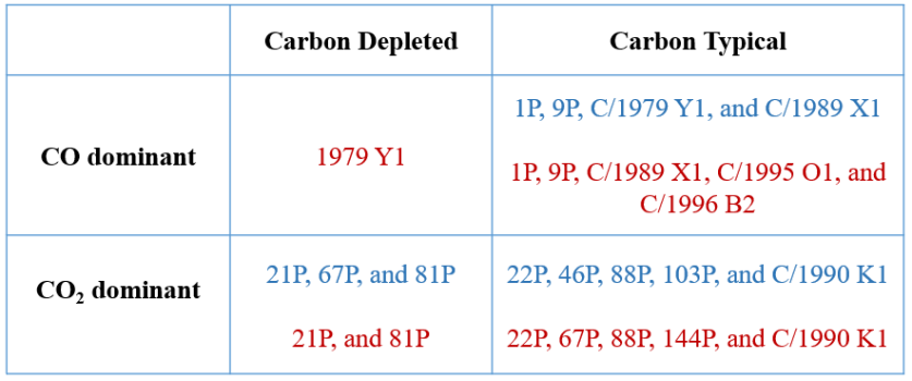
Figure 10: The classification of carbon richness (depleted/typical) is compared against the CO and CO₂-dominance from this paper. The blue text in the box uses the categorization of depletion or typical carbon content from A’Hearn et al. (1995), while the red is the categorization from Cochran et al. (2012).

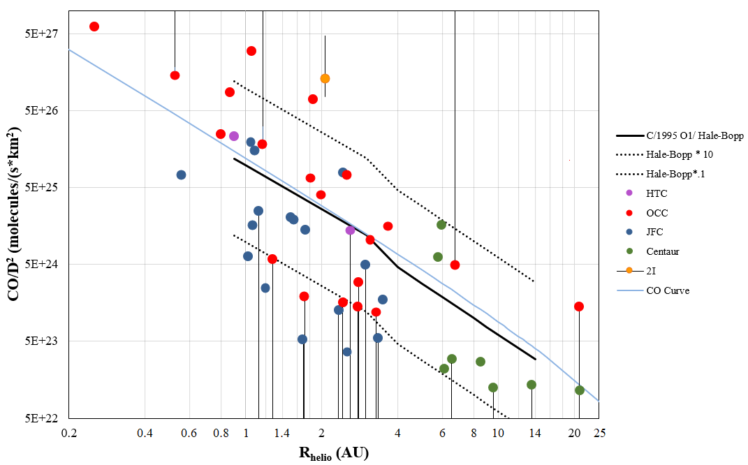
Figure 11: Here we plot specific production rate per unit of area, Q_CO/D², vs. heliocentric distance. Overlaid in a blue line is the sublimation curve from Sekanina (1992) for CO for a comet with a diameter of 32 km. When observed over 1 to 2 au, OCCs produce significantly more CO per surface area than most JFCs. One Centaur (29P) shows elevated productivity for its size at 6 au, while all other Centaurs measured to date produce very little CO for their size, or none at all. This could be a response to decreased solar heating of the Centaurs at larger distances. C/2017 K2’s CO detection at $\sim$ 6 au and diameter upper limits indicate that the this OCC is producing high amounts of CO for its size, possibly out-producing Hale-Bopp and 29P at this distance. For comparison, the specific production rate for C/1995 O1 Hale-Bopp is shown in solid black line.

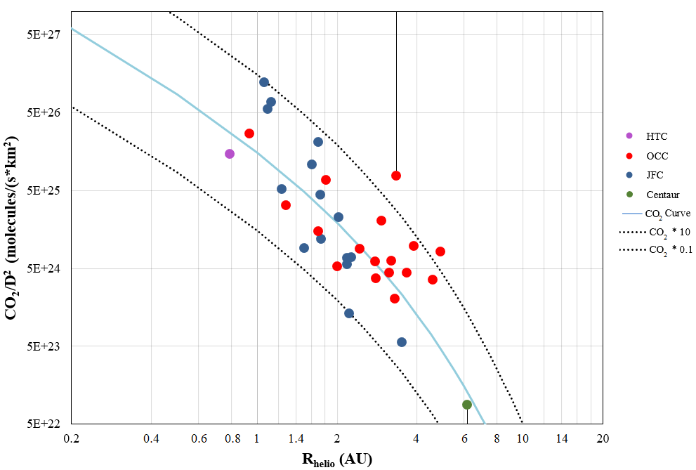
Figure 12: Here we plot specific production rate per unit of area, Q${}_{CO_{2}}$/D², vs. heliocentric distance. Overlaid in a blue line is the sublimation curve from Sekanina (1992) for $CO_{2}$ for a comet with a diameter of 10 km. The dotted lines above and below the CO₂ curve are for the cases when there is ten times more CO₂ production and a tenth of the CO₂ production, respectively.

3.7 Active fraction areas for CO and CO₂

We normalized CO production rates for surface area (assuming a spherical shape) for comets using published diameters and plotted them against heliocentric distance (Figure 11). The references for the diameters and the CO productions are in Table 5.1. Three of our comets have significant upper limits for diameters: C/2001 A2, C/2012 S1, and C/2017 K2.

In Figure 11, interstellar comet 2I Borisov produces more than 10 times the CO production of C/1995 Hale-Bopp for its surface area and is similar to some other OCCs from our solar system around the distance it was observed. Distantly active comet C/2017 K2 is also in the graph where it shows significant activity at large distances, even above the activity level of C/1995 O1 Hale-Bopp, despite its size not being determined yet. If its nucleus is even smaller than the upper limits used, then C/2017 K2’s will have an even higher specific CO production rate for its surface area.

A CO vaporization curve is superimposed in Figure 11, which is the sublimation rate as a function of heliocentric distance for a comet with a 32 km diameter. Interestingly, when looking at 1-4 au in Figure 11, the CO specific production rates of most JFCs are an order of magnitude lower than C/1995 O1 Hale-Bopp. In contrast, within 1 au, the CO specific production rates for all OCCs are located above the C/1995 O1 line, and at distances above 1 au most OCCs show less activity. The two Halley type comets are similar to the C/1995 O1 Hale-Bopp line, which would support the idea that some HTCs originated from the Oort Cloud (Levison, 1996). Centaurs are dispersed with a couple of values from 29P (the lowest from quiescent activity and the highest from outburst activity), much lower detections from Centaurs Echeclus and Chiron, and several upper limits for other Centaurs which are significantly lower than C/1995 O1 Hale-Bopp. The lower CO/D² values for the Centaurs could either be from incorporation of less CO in the nucleus, or inhibition of CO outgassing at these large distances (Wierzchos et al., 2017).

Figure 12 shows the normalized CO₂ production rates for surface area (assuming a spherical shape) with their respective references listed in Table 5.1. Comet C/2012 S1 is the only comet in this figure with an upper limit diameter. Figure 12 has CO₂ vaporization curve for a comet with a 10 km diameter superimposed on the graph. Unlike Figure 11, in Figure 12 both JFCs and OCCs follow the behavior of the CO₂ sublimation curve with less scatter. There is only one data point in the Q${}_{CO_{2}}$/D² graph representing HTCs and Centaurs so we can not say anything definitive about either of those classes of objects, other than both appear to fall very near the sublimation line.

4 Individual comets

Next we provide additional background information, context, and any additional analysis steps we carried out for the comets analyzed for contemporaneous CO and CO₂ measurements. Comets 144P, C/1989 X1, C/1990 K1, C/2006 Q1, C/2007 Q3, and C/2008 Q3 do not have individual subsections. The telescopes used to obtain the CO and CO₂ of the individual comets here are listed in Table 2.1.

4.1 1P/Halley

We used CO and CO₂ production rates obtained from the Vega spacecraft infrared spectroscopy measurements (Combes et al., 1988). Production rates were also inferred from ultraviolet spectra of CO with similar numbers, but we instead use infrared spectroscopy because of the direct simultaneous measurements of CO and CO₂. 1P/Halley is CO-dominant compared to CO₂, which might be consistent with Halley retaining much of its natal abundances.

4.2 9P/Tempel 1

9P is a notably potato-shaped comet visited by Deep Impact and Stardust spacecraft. It has a short orbital period of six years and a 6 km diameter, with circular features on its surface consistent with a layered nucleus (Thomas et al., 2007). We use the pre-impact measurements of CO and CO₂ measured by Deep Impact and HST. The Deep Impact HRI-IR spectrometer detected CO₂ and H₂O emission on July 4, ten minutes before impact, but did not detect CO (Feaga et al., 2007). The HST ACS Solar Blind Channel detected CO 4^th Positive gaseous emission a day earlier, which we used for CO production rate (Feldman et al., 2006).

For comparison, the pre-impact H₂O production rate of 5 $\times$ 10²⁷ molecules sec^-1 derived from OH photometry also on July 4 Schleicher (2007) is in good agreement with the 4.6 $\times$ 10²⁷ molecules sec^-1 derived by Feaga et al. (2007) on the same day that we used.

The CO/CO₂ ratio is 1.88 at R_Helio = 1.51 au (pre-impact), and it is the only JFC to be have a CO-dominated coma instead of CO₂.

Interestingly, post-impact IR measurements (Mumma et al., 2005) show a lower CO/H₂O ratio than the pre-impact values. It is not clear what causes these differences (different techniques or pre-to-post impact changes), but if the IR values are accurate, and CO₂ production relative to water remained constant, then it is possible that 9P’s coma may not always be CO dominated compared to CO₂.

4.3 21P/Giacobini-Zinner

This well-studied comet has been observed over many apparitions by several spacecraft, ICE, Pioneer Venus 1, and many ground-based telescopes. It is also considered by many to be the prototypical carbon-depleted comet (Moulane et al., 2020; Roth et al., 2020).

We calculated the CO/CO₂ mixing ratio using a combination of the individual CO and H₂O production rates derived from IR data (Roth et al., 2020) and a CO₂/H₂O production rate ratio that was inferred from analysis of the green to red doublet ratio (G/R) of forbidden oxygen that was obtained on October 3, 2018 (Shinnaka et al., 2020). We then calculated the CO/CO₂ mixing ratio using the CO₂/H₂O ratio, taken on October 3, 2018 (Shinnaka et al., 2020), and the H₂O and CO detections observed seven days later on October 10, 2018 (Roth et al., 2020), according to:

$${{Q_{CO}}\over{Q_{CO_{2}}}}={{{Q_{CO}}\over{Q_{H_{2}O}}}\times{{Q_{H_{2}O}}\over{Q_{CO_{2}}}}}$$ (4)

The Q_CO/Q${}_{CO_{2}}$ ratio = 0.114, which makes it a CO₂-dominant comet, like 8 out of 9 JFCs in our sample.

4.4 22P/Kopff

22P is a highly active JFC (Lamy et al., 2002) and a dynamical study indicates that it recently transferred from the Centaur to JFC region, possibly within the last $\sim$ 100 years (Pozuelos et al., 2014). The CO/CO₂ ratio is an upper limit of 0.15 (Ootsubo et al., 2012), which makes it a CO₂-dominant comet, like 8 out of 9 JFCs in our study.

4.5 29P/Schwassmann-Wachmann

29P was previously considered by many to be a JFC, however orbital dynamical studies showed that 29P is a transitional object between Centaurs and JFCs, and is the first known inhabitant of the “Gateway” transition region just beyond Jupiter’s orbital distance from the Sun (Sarid et al., 2019). 29P is also unusual in that it has a nearly circular orbit at $\sim$ 6 AU, and with an ever-present dust coma, likely driven by CO outgassing (Senay & Jewitt, 1994). In addition to its constant, low-variable, quiescent activity, it has has several substantial outbursts per year (Trigo-Rodríguez et al., 2008; Womack et al., 2017; Wierzchos & Womack, 2020) and a persistent 24 $\mu$m “wing” feature that is largely created by solar radiation pressure on micron-sized grains (Schambeau et al., 2015).

CO is readily measured at millimeter- and infrared-wavelengths, but CO₂ emission has not been detected yet in 29P. Ootsubo et al. (2012) reported strong upper limits obtained of its 4.67 $\mu$m band with AKARI which yields an average production rate ratio for CO/CO₂ $>$ 84, the highest value in our dataset.

In order to further quantify the CO₂ contribution to the coma, we infer the CO₂ production rate following the method described in Section 2.2. To carry out this analysis, we used the total CO+CO₂ emission recorded by Spitzer (Reach et al., 2013) and NEOWISE (Bauer et al., 2015) infrared space telescopes, CO mm-wavelength data obtained with the IRAM 30-m (Bockelée-Morvan et al., 2022), and visible magnitude data (Trigo-Rodríguez et al., 2010), all of which were observed during the first half of 2010.

The independent CO data were not obtained simultaneously with the Spitzer data, however, independent visual monitoring showed no evidence of major dust outbursts within a few days of the NEOWISE data (Trigo-Rodríguez et al., 2010). This Centaur is continuously active and exhibits a relatively constant amount of CO emission and dust, except when in outbursting mode when it increases significantly. A recent study showed that outbursts of CO gas and dust in 29P do not always correlate in time Wierzchos & Womack (2020), so caution is warranted.

The IRAM 30-m observations did not showed gas production rates that varied little over their five observing dates from 2010 February 12 to May 29 with an average of Q_CO = 4.6 x 10²⁸ mol s^-1. The visual lightcurve data show no evidence of a dust outburst at the time the Spitzer data were obtained on 2010 Jan 25, so we use the average CO production rate from IRAM for Q_independent in Equation 1, and 11.6 for the ratio of the fluorescence efficiencies (Equation 2) to derive Q${}_{CO_{2}}$ = (5$\pm$3)x10²⁶ mol s^-1 and a mixing ratio of CO/CO₂ $\sim$ 92 using the Spitzer and IRAM data. Within the uncertainties, this is consistent with the AKARI spectroscopic measurements of Q${}_{CO_{2}}$ $<$ 3.5x10²⁶ molecules s^-1 and CO/CO₂ $>$ 84 obtained on 2009 Nov 19 (Ootsubo et al., 2012). The combined Spitzer and IRAM analysis confirm that CO₂ emission has a very small presence in 29P’s coma, approximately 1% of CO and 14% of H₂O.

The same process was applied to the NEOWISE data, which was also obtained during spring 2010 near when CO was also observed with IRAM. This leads to a Q${}_{CO_{2}}$ $\sim$ 3x10²⁷ mol s^-1. This is $\sim$ eight times lower than the AKARI lower limit in Nov 2009 and the value we derive from Spitzer in Jan 2010, and the mixing ratio is CO/CO₂ $\sim$ 16. Although more CO₂ is inferred from the NEOWISE data, they are still consistent with CO₂ emission being a minor contributor to 29P’s coma.

29P clearly has the most CO-dominated coma compared to CO₂ in this study. Further studies may clarify how much of this difference is due to intrinsic chemical composition of its nucleus, and how much can be attributed to its relatively far distance from the Sun, which might favor CO release over the less volatile CO₂ (see Section 3.1). A recent study proposes that the preferential release of CO over CO₂ in 29P can be explained largely by amorphous water ice converting to the crystalline state upon increased heating in its relatively new orbit (Lisse et al. 2022, under review).

4.6 46P/Wirtanen

CO₂ emission was not directly detected for 46P, but its relative abundance to water was inferred through analysis of forbidden oxygen (see Section 2.1), as was a measurement of the water production rate. Three days later, a H₂O production rate was also measured with infrared spectroscopy, along with an upper limit to the CO emission. The water production rates obtained on both days (through [OI] and infrared techniques) agreed within 3.6% and was used to extract a CO₂ production rate. We assume that the production rates for CO and CO₂ were also stable over these three days (cf. McKay et al. (2021).)

4.7 67P/Churyumov–Gerasimenko

We used simultaneous mass spectroscopy measurements for CO and CO₂ from (Combi et al., 2020). Over time, the CO/CO₂ production rate ratio spans all three regions (CO-dominant, CO₂-dominant, and equal parts). The start of Rosetta’s observations of 67P recorded higher CO than CO₂. Shortly after, while 67P was still traveling inward, the CO and CO₂ production rates were almost comparable with the CO₂ production detected being slightly greater than the CO production. After reaching perihelion the CO₂ production was greater than the CO production recorded (Combi et al., 2020). The CO and CO₂ presented in the figures and table are representative of the production rates at the observed times, and not outliers. Although numerous measurements are available throughout its perihelion passage, we use just three values to represent CO/CO₂ behavior of 67P at 1.2 au, 2.0 au, and 3.5 au.

This comet is also known for its rubber duck-like shape, thought to have been the result of two cometesimals colliding. It is sometimes considered as two objects since the interior layers of the lobes are oriented in different directions (Massironi et al., 2015). 67P was measured to be alternately CO and CO₂-dominated during its inward journey, most of this variation was determined to be a seasonal effect and partially due to compositional differences between the two lobes of the nucleus (Fougere et al., 2016; Hässig et al., 2015; Combi et al., 2020; Fornasier et al., 2021). Overall it was considered to be a CO₂-dominant coma where the average CO/CO₂ production rate ratio in the coma was 0.67 (Combi et al., 2020). Interestingly, the smaller lobe has a CO₂ spot that is active while the waist, or neck, of 67P has shown more H₂O activity and not as much CO₂. The changes in the activity of the volatiles are attributed to seasonal effects and heliocentric distance (Fougere et al., 2016; Combi et al., 2020).

4.8 81P/Wild 2

In 1974, 81P passed within 0.006 au of Jupiter which dramatically changed its orbit, and simulations indicate that it was previously in a Centaur-like orbit, and that in $\sim$ 8,000 years, 81P may no longer be a JFC (Królikowska & Szutowicz, 2006). Thus, despite its current JFC designation, 81P may be relatively unprocessed compared to many other JFCs. It has Q_CO/Q${}_{CO_{2}}$ $<$ 0.26 (Ootsubo et al., 2012), which puts it in the CO₂-dominant category, similar to 8 out 9 JFCs observed for CO and CO₂.

4.9 88P/Howell

Although measured with multiple techniques, the most constraining measurement of the relative amounts of CO and CO₂ in 88P’s coma is an upper limit of Q_CO/Q${}_{CO_{2}}$ $<$ 0.31 derived from AKARI space telescope measurements at 1.73 au on July 3, 2009 based on a detection of Q${}_{CO_{2}}$ = $8.65\times 10^{26}$ molecules/sec and an upper limit for CO (Ootsubo et al., 2012). Two prominent jets were observed on 88P at 1.47 au a month later on Aug 8 with Spitzer IRAC, and CO₂ was attributed as the main driver of activity for the jets (Reach et al., 2013).

4.10 103P/Hartley 2

Peanut-shaped 103P was visited by the Deep Impact spacecraft, which found it had hyperactive behavior, meaning that it released larger amounts of H₂O than expected for the nucleus’ surface area (A’Hearn et al., 2011). Other known hyperactive comets include 21P and 46P.

We used the CO₂ detection obtained with the HRI-IR spectrometer (A’Hearn et al., 2011) and the CO measured from the 4^th Positive Bands with HST (Weaver et al., 2011). There was an upper limit obtained for the CO₂ (Weaver et al., 2011) (<2 x 10²⁷ molecules sec${}^{-}1$) and CO was not detected with the HRI-IR (Feaga et al., 2014). The upper limit from Weaver et al. (2011) is in agreement with the detection from A’Hearn et al. (2011).

The CO/CO₂ production rate ratio is 0.01, which makes it the most CO₂-dominated coma in our study. CO₂ is the primary driver of activity in 103P and likely contributed to dragging out chunks of nearly pure water-ice, which then sublimated in the coma to provide a large fraction of the total H₂O gaseous output of the comet (A’Hearn et al., 2012).

4.11 C/1979 Y1 Bradfield

C/1979 Y1 was the first comet for which UV measurements were taken over a range of heliocentric distances (0.71 au to 1.55 au) (Levasseur-Regourd, 1988). The UV measurements we used are from Feldman et al. (1997), where the CO was obtained via the 4^th Positive band, and the CO₂ production rate was calculated from CO Cameron Band emission. In Figure 4 C/1979 Y1 Bradfield has a smaller semi-major axis than other OCCs in the figure, and with a CO/CO₂ = 1.00 it does not follow the behavior of other OCCs that have had multiple trips to thine inner solar system and have CO-dominant comae. It is possible that the low CO/CO₂ C/1979 Y1 could be due to the inhibition of CO by a chemical or morphological feature on the comet, or that what we see is the result of the small sample size of OCCs.

The CO/CO₂ mixing ratio is 1.00, consistent with comparable amounts of CO and CO₂ in the coma. Upon discovery, it was considered to be one of the gassiest comets, comparable to 2P/Encke, with a gas to dust ratio of 22 at 0.8 au (A’Hearn et al., 1981). Although categorized as coming from the Oort Cloud, its orbital characteristics may be consistent with a Halley type comets (A’Hearn et al., 1995). For comparison, comet Halley had a ratio of $\sim$ 3.

4.12 C/1995 O1 Hale-Bopp

C/1995 O1 Hale-Bopp was well-studied due to its long-term bright behavior starting upon discovery in 1995. Notable structural features observed in C/1995 O1 Hale-Bopp include three distinct tails: gas, dust, and sodium (Cremonese et al., 1997), jets, and curved features in the dust coma (Warell et al., 1999; Braunstein et al., 1997; Womack et al., 2021). The CO/CO₂ ratios are observed for multiple dates at large heliocentric distances and all of the ratios show that C/1995 O1 Hale-Bopp had far more CO than CO₂ in its coma. All measurements of CO₂ were made when the comet was beyond 3 au. There was CO₂ obtained from CO Cameron bands with the HST FOS on September 23, 1996 around the same time as one of the observations from ISO (September 26, 1996). The CO₂ from HST was 8.8 x 10²⁸ and the from ISO was 7.4 x 10²⁸ (Crovisier et al., 1999a). We also see more data, from Table 5.1 and in Figure 5, showing that CO/H₂O was seen in higher amounts compared to most other comets at the same distance, especially at lower heliocentric distances.

4.13 C/1996 B2 Hyakutake

C/1996 B2 Hyakutake is among the brightest comets in the last century and it was discovered about six months after C/1995 O1 Hale-Bopp. C/1996 B2 was the first comet where ethane was detected and in abundance (Mumma et al., 1996).

The CO/CO₂ ratio is 2.83 and was measured via CO 4^th Positive band and confirmed with CO Cameron band measurements (McPhate, 1999). Given the high CO abundance, the CO Cameron bands were attributed to CO instead of CO₂.

4.14 C/2006 OF2 Broughton

Comet C/2006 OF2 Broughton was identified as a carbon-chain depleted comet based on its CN and C₃ abundances (Kulyk et al., 2021). CO was not detected, but CO₂ was detected with the AKARI telescope, so the CO/CO₂ ratios obtained are upper limits, with the most conservative (highest) value being $<$0.45 (Ootsubo et al., 2012), consistent with a CO₂-dominated coma.

4.15 C/2006 W3 Christensen

This distantly active comet never approached closer than $\sim$ 3 au of the Sun during its perihelion passage and was found to be rich in molecules more volatile than water and the distant CO production was proposed to be largely released during the crystallization of amorphous water ice near the nucleus surface (Bockelée-Morvan et al., 2010; Prialnik et al., 2004). CO and CO₂ emission was detected by AKARI with values ranging from Q_CO/Q${}_{CO_{2}}$ = 2.3 to 3.5. This high ratio was attributed to being at least partly due to insufficient sublimation of CO₂ at relatively large distances of 3.13 and 3.66 au from the Sun (Ootsubo et al., 2012).

4.16 C/2007 N3 Lulin

C/2007 N3 is a dynamically new comet with two near polar jets and a morphology that is different from that of the water outgassing, and thus was proposed to have either CO₂ or CO as the main drivers of activity (Gibb et al., 2012a; Bair et al., 2018). Given that Q${}_{CO_{2}}$ $>>$ Q_CO from the AKARI measurements, it seems that the jets were most likely driven by CO₂ outgassing. Comparison with water production rates also shows that CO was present in very small amounts with the highest abundance ratio reaching 2.2%. In this coma very low relative to H₂O (Ootsubo et al., 2012; Gibb et al., 2012b), see Table 5.1, and Table 5.1.

4.17 C/2009 P1 Garradd

The HRI-IR detected for both CO and CO₂ emission in C/2009 P1 during its extended EPOXI mission (A’Hearn et al., 2011; Feaga et al., 2014).

The CO/CO₂ ratio was 7.44, corresponding to a CO-dominant coma. C/2009 P1 Garradd’s active fraction of the nucleus exceeded 50 % (Boissier et al., 2013) and the CO production significantly increased after perihelion (Bodewits et al., 2014; Feaga et al., 2014).

4.18 C/2012 S1 ISON

The CO₂ production rate for comet C/2012 S1 was calculated using Spitzer 4.5 $\mu$m combined CO+CO₂ images (Lisse et al., 2013) and an independently modeled CO production rate that agreed with estimates from CO from HST and a marginal CO detection at mm-wavelengths. Modeling showed that CO₂ was an unlikely match to the Spitzer excess emission (Meech et al., 2013) and instead the activity was probably driven by CO. We used this CO value to extract a CO₂ production rate from the Spitzer measurements.

4.19 C/2016 R2 PanSTARRS

C/2016 R2 pre-perihelion observations were taken from Arizona Radio Observatory 10-m SMT (CO J=2-1) on February 13, 2018 at 5:16 UT and with Spitzer IRAC on February 12, 2018 at 18:22 UT (CO₂+CO), with a difference of $\sim$ 11 hours between them. The post-perihelion observations were taken on June 12, 2019 with the ARO SMT and on June 10, 2019 with Spitzer IRAC so the date between them June 11, 2019, was used to represent the data. CO detections observed pre-perihelion taken a couple weeks before by the IRTF iShell were in agreement with the CO obtained with the SMT (McKay et al., 2019), but since we were trying to use the measurements that were taken the closest together in time we use the CO from the SMT.

Unlike other comets that are mainly composed of H₂O, the dominant volatiles in comet C/2016 R2 are N₂ and CO (McKay et al., 2019). Interestingly, despite extraordinarily high fractional abundances of CO and CO₂ with water, the CO/CO₂ (determined by Equations 1 and 2) ratios are more similar to what other Oort Cloud comets had at similar distances (Figure 2). Due to its distinct molecular composition, it is believed that C/2016 R2 formed further out than where H₂O rich comets formed and the likelihood of observing a similar comet to C/2016 R2 is low (Mousis et al., 2021). The factor of 3.6 increase in the CO/CO₂ ratio from pre-perihelion to post-perihelion looks like fellow OCC, C/1995 O1 Hale-Bopp. Not only is this comet CO rich in the coma, it is very H₂O poor, and some have wondered whether it could have formed beyond the N₂ ice line or be a fragment from a TNO (Wierzchos & Womack, 2018; Biver et al., 2018).

C/2016 R2 also has the highest fractional abundances of CO/H₂O and CO₂/H₂O distinct from composition from all other comets. Even the interstellar comet, 2I/Borisov, only had a CO/H₂O ratio of 1.425 at 2.12 au while C/2016 R2’s CO/H₂O ratio was 177.42 at 2.76 au.

5 Summary and Conclusions

We compiled a comprehensive survey of published contemporaneous CO and CO₂ production rates in 25 comets, and we include water production rates and nucleus diameters when available. We supplemented this analysis with additional measurements of water, CO, and CO₂. From this dataset we analyzed key production rate ratios, including the volatile C/O ratio, and searched for possible correlations with heliocentric distance, orbital families, and nucleus surface area. Key findings are listed below, including some interesting trends, which can be tested with future observations.

1. We infer Q${}_{CO_{2}}$ = (5$\pm$3)x10²⁶ mol s^-1 for 29P using contemporaneous data from the Spitzer and the IRAM 30-m telescopes. This value indicates that CO₂ is present in the Centaur’s coma at the level of $\sim$ 1% of CO and 5% of H₂O. 29P clearly has the highest CO/CO₂ mixing ratio in this study. It is not clear how much of this difference between CO and CO₂ release is due to chemical composition of the nucleus and how much can be attributed to preferential CO release over the less volatile CO₂ at $\sim$ 6 au from the Sun.

2. Collectively, approximately half of the 25 comets had more CO₂ than CO in their coma, one third were CO-dominated, and about a tenth had comparable amounts of CO and CO₂.

3. Eight of the nine JFCs had CO₂-dominated comae, which may be partly explained by preferential loss of CO vs. CO₂ over millenia.

4. All six comets on their first trip from the Oort Cloud to the inner solar system (dynamically new) produced more CO₂ than CO when within 2.5 au of the Sun, while the remaining eight comets, which were on their second or later trip, produced more CO at this distance. DN comets produce more CO₂ relative to CO than the other Oort Cloud Comets that have made multiple passes through the inner solar system. There may also be a trend where the Q_CO/Q${}_{CO_{2}}$ ratio increases with dynamical age, as first pointed out by A’Hearn et al. (2012). These results are inconsistent with models that predict that the least processed comets should have more CO than CO₂ and raises questions about comet formation and evolution models. A low CO/CO₂ production rate ratio for dynamically new comets may instead be explained by a model that includes galactic cosmic rays processing that alters the ice composition down to meters below the surface, resulting in CO-depletion with respect to CO₂ (Gronoff et al., 2020; Maggiolo et al., 2020). This highly processed layer is then eroded during the first perihelion passage, revealing relatively fresher surface layers with pockets of CO ice that are liberated during subsequent passages.

5. All comae observed beyond 3.5 au were dominated by CO. This could be due to the higher volatility of CO, but a selection effect due to the small sample size of active comets beyond 3.5 au could also be a contributing factor. Based on the results of this study, when independent measurements are not possible for both species for an active comet beyond 3.5 au, it may be appropriate to assume that the dominant volatile is CO rather than CO₂.

6. Given the possible trend of increasing Q_CO/Q${}_{CO_{2}}$ with larger heliocentric distance, and the lack of JFC measurements of these species beyond $\sim$ 3.5 au, there may be a selection effect which leads to the lower Q_CO/Q${}_{CO_{2}}$ in JFCs. Many additional measurements of Q_CO/Q${}_{CO_{2}}$ in JFCs at larger distances, especially beyond 4 au, are needed to determine the contributions due to thermal heating and chemical composition of the nucleus as primary contributors for the apparent difference between the JFC and OCC comae.

7. If the trend of Q${}_{CO_{2}}$ $\geq$ Q_CO for dynamically new comets holds (Section 3.4), then we anticipate that the incoming DN comet C/2017 K2 (PanSTARRS) should produce more CO₂ than CO when it is near perihelion.

8. For comets within 2.5 au, the CO/H₂O production rate ratio has a median of 3 ± 1%, with a range from 0.3% to 26%. For CO₂/H₂O, the median is higher, 12 ± 2% with a range from 2% to 30%. The production rate ratio for CO may change slope at $\sim$ 2.5-3.0 au, where water ice sublimation noticeably changes its efficiency.

9. For all comets from 0.7 to 4.6 au, Q${}_{CO_{2}}$/Q${}_{H_{2}O}$ shows a much tighter correlation (less scatter) with respect to heliocentric distance than does Q_CO/Q${}_{H_{2}O}$. This may mean that the production of CO₂ and CO has significantly different mechanisms over this range, and that CO₂ outgassing may be more intimately tied to water production than CO is. In contrast, the fractional CO production rate has a much stronger response to solar heating than does CO₂, which is consistent with CO being much more volatile.

10. The median production rate ratios of (Q_CO + Q${}_{CO_{2}}$)/Q${}_{H_{2}O}$ for all comets within 2.5 au is 18 ± 4%, although there is some substantial deviation from this value for a few comets. This indicates that the total amounts of CO and CO₂ produced within 2.5 au is conserved for most comets and represents $\sim$ 20% of the total volatile component, as proposed by A’Hearn et al. (2012); Lisse et al. (2021). This may support the theories that comets retain a strong amount of their natal composition.

11. When observed over the heliocentric distance range of 1 au to 2 au, most Oort Cloud comets produce significantly more CO per surface area than JFCs. No distinction is seen for CO₂ between the two groups of comets.

12. We computed the carbon-to-oxygen ratio for the gaseous component using contemporaneous production rates of CO, CO₂, and H₂O in 18 comets, the largest sources of carbon and oxygen in comae. We find C/O_average $\sim$ 15% and C/O_median $\sim$ 13%, which is consistent with most comets forming within the CO snow line (i.e., C/O $<$ 0.2) (Seligman et al., 2022). A notable exception is the anomalous C/2016 R2, with C/O $\sim$ 0.9, which can be explained by forming farther out, possibly beyond the CO snow line. We see no distinction between the JFCs and OCCs with respect to C/O ratios. This may be explained by models which predict that both Kuiper Belt and Oort Cloud reservoirs have similar origins and that they both formed within the region of the giant planets (i.e. 5-30 au).

5.1 Large Tables

Table 4: Contemporaneous CO, CO₂, and H₂O Measurements in Comets

Comet	Date	RHelio	True Anomaly	QCO	Q${}_{CO_{2}}$	Q${}_{H_{2}O}$	QCO/Q${}_{CO_{2}}$	QCO/Q${}_{H_{2}O}$	Q${}_{CO_{2}}$/Q${}_{H_{2}O}$	1/$a_{0}$	Ref.
	(YYYY/MM/DD)	(AU)	(degrees)	$10^{26}$ sec-1	$10^{26}$ sec-1	$10^{26}$ sec-1				$10^{-4}$ AU-1
1P/Halley	1986/03/06	0.79	61	500.00	180.00	4500.0	2.78	0.110	0.04	-	2
9P/Tempel 1	2005/07/03	1.51	359	5.00	-	-	-	-	-	-	6
9P/Tempel 1	2005/07/04	1.51	359	-	3.20	46.0	1.88	0.130	0.07	-	5
21P/G-Z	2018/10/03	1.07	28	-	-	-	-	-	0.11	-	21
21P/G-Z	2018/10/10	1.10	36	2.55	-	203.7	0.11	0.013	-	-	20
22P/Kopff	2009/04/22	1.61	340	$<$1.65	10.96	59.4	$<$0.15	$<$0.030	0.18	-	1
29P/S-W 1	2009/11/18	6.18	135	291.5	$<$3.5	67.8	$>$83.2	4.630	$<$0.05	-	1
46P/Wirtanen	2019/01/08	1.11	29	-	8.55	-	$<$0.04	-	0.15	-	11
46P/Wirtanen	2019/01/11	1.13	33	$<$0.31	-	57.0	$<$0.04	$<$0.005	-	-	11
67P/C-G	2014/08/23	3.50	229	0.21	0.07	0.5	3.06	0.450	0.15	-	12
67P/C-G	2015/08/13	1.24	359	4.78	6.26	158.1	0.76	0.030	0.04	-	12
67P/C-G	2016/01/02	2.03	89	0.36	2.71	11.5	0.13	0.030	0.24	-	12
81P/Wild 2	2009/12/14	1.74	320	$<$2.24	8.63	60.0	$<$0.26	$<$0.040	0.14	-	1
88P/Howell	2009/07/03	1.73	294	$<$2.72	8.65	33.5	$<$0.31	$<$0.080	0.26	-	1
103P/Hartley 2	2010/11/02	1.06	8	-	20.00	100.0	0.01	0.003	0.20	-	4
103P/Hartley 2	2010/11/04	1.06	8	0.26	-	-	-	-	-	-	3
144P/Kushida	2009/04/18	1.70	53	$<$1.14	5.57	37.6	$<$0.20	$<$0.030	0.15	-	1
C/1979 Y1	1980/01/10	0.71	56	51.00	51.00	1460.0	1.00	0.030	0.03	232.7	13,15
C/1989 X1	1990/05/09	0.83	99	17.00	21.00	1020.0	0.81	0.020	0.02	0.3	13,15
C/1990 K1	1990/08/26	1.38	291	101.00	170.00	2480.0.0	0.59	0.040	0.07	0.7	13,15
C/1990 K1	1990/09/18	1.13	311	168.00	268.00	2010.0	0.63	0.080	0.13	0.7	13,15
C/1995 O1	1996/04/27	4.58	233	700.00	130.00	131.0	5.38	5.340	0.99	38.4	7,16
C/1995 O1	1996/09/26	2.93	248	2300.00	740.00	3300.0	3.11	0.700	0.22	38.4	7
C/1995 O1	1997/12/29	3.89	122	1500.00	350.00	280.0	4.29	5.360	1.25	38.4	7
C/1995 O1	1998/04/06	4.90	129	3000.00	300.00	-	10.00	-	-	38.4	7
C/1996 B2	1996/06/02	0.94	170	180.00	60.00	1530	2.83	0.111	0.04	15.5	17
C/2006 OF2	2008/09/16	2.43	0	$<$2.52	13.97	61.2	$<$0.18	$<$0.040	0.23	0.2	1
C/2006 OF2	2009/03/28	3.20	59	$<$4.46	9.90	17.0	$<$0.45	$<$0.260	0.58	0.2	1
C/2006 Q1	2008/06/03	2.78	351	$<$3.67	16.19	36.3	$<$0.23	$<$0.100	0.45	0.4	1
C/2006 W3	2008/12/21	3.66	315	299.30	84.59	83.0	3.54	3.610	1.02	3.7	1
C/2006 W3	2009/06/16	3.13	355	197.70	84.66	201.0	2.34	0.980	0.42	3.7	1
C/2007 N3	2009/02/05	1.28	26	$<$8.67	48.48	409.1	$<$0.18	$<$0.020	0.12	0.3	1
C/2007 N3	2009/03/30	1.70	64	$<$2.86	22.42	223.8	$<$0.13	$<$0.010	0.10	0.3	1
C/2007 Q3	2009/03/03	3.29	292	$<$3.97	6.95	39.8	$<$0.57	$<$0.100	0.17	0.3	1
C/2008 Q3	2009/07/05	1.81	7	29.30	31.04	112.0	0.94	0.260	0.28	2.5	1
C/2009 P1	2012/03/26	2.00	56	290.00	39.00	460.0	7.44	0.630	0.08	4.2	9
C/2012 S1	2013/06/13	3.34	187	7.00	1.21	$<$100.0	5.79	*	*	1.2	10,19
C/2016 R2	2018/02/12	2.76	332	-	90.50	-	-	-	-	11.7	8
C/2016 R2	2018/02/13	2.76	333	550.00	-	-	6.08	-	-	11.7	8
C/2016 R2	2018/02/21	2.73	335	-	-	3.1	-	177.420	29.19	11.7	8
C/2016 R2	2019/06/10	4.72	84	-	6.21	-	19.00	-	-	11.7	14
C/2016 R2	2019/06/12	4.73	84	118.00	-	-	-	-	-	11.7	18

References. — 1: Ootsubo et al. (2012), 2: Combes et al. (1988), 3: Weaver et al. (2011), 4: A’Hearn et al. (2011), 5: Feaga et al. (2007), 6: Feldman et al. (2006), 7: Crovisier et al. (1999a), 8: McKay et al. (2019), 9: Feaga et al. (2014), 10: Lisse et al. (2013), 11: McKay et al. (2021), 12: Combi et al. (2020), 13: Feldman et al. (1997), 14: private communication with Adam McKay (Spitzer CO proxy), 15: Tozzi et al. (1998), 16: Colom et al. (1997) OH production given as a proxy for H₂O, 17: McPhate (1999) H₂O is derived from the OH band, 18: Wierzchos (2019), 19: Meech et al. (2013), 20:Roth et al. (2020), 21: Shinnaka et al. (2020) The 1/$a_{0}$ values are from the MPC database and are used to construct Figure 4. *: The water production is an upper limit the production rate ratios.

Table 5: Additional CO, CO₂, and H₂O Measurements in Comets

Comet	Date	RHelio	Q${}_{H_{2}O}$	QCO	Q${}_{CO_{2}}$	QCO/Q${}_{H_{2}O}$	Ref.
	(YYYY/MM/DD)	(AU)	$10^{26}$ sec-1	$10^{26}$ sec-1	$10^{26}$ sec-1	or Q${}_{CO_{2}}$/Q${}_{H_{2}O}$
19P/Borrelly	2008/12/30	2.19	6.4	-	1.6	0.250	16
64P/Swift–Gehrels	2009/11/23	2.27	6.9	-	1.5	0.220	16
103P/Hartley 2	1997/12/31	1.04	-	-	12.0	-	1
103P/Hartley 2	1998/01/01	1.04	124.0	-	-	0.097	1
116P/Wild 4	2009/05/16	2.22	15.8	-	0.9	0.056	16
118P/Shoemaker–Levy 4	2009/09/08	2.18	10.0	-	3.0	0.300	16
157P/Tritton	2009/12/30	1.48	4.5	-	0.3	0.069	16
C/2007 G1 (LINEAR)	2008/08/20	2.80	18.4	-	4.2	0.230	16
8P/Tuttle	2008/01/27	1.03	544.0	2.4	-	0.004	24
8P/Tuttle	2007/12/23	1.15	212.8	$<$0.8	-	$<$0.004	25
21P/Giacobini–Zinner	1998/10/02	1.25	320.0	33.0	-	0.100	27
21P/Giacobini–Zinner	2018/07/30	1.17	231.6	5.5	-	0.024	28
21P/Giacobini–Zinner	2018/10/07	1.09	258.3	3.7	-	0.014	28
41P/Tuttle–Giacobini–Kresák	2017/04/26	1.06	50.0	$<$8.5	-	$<$0.170	28
45P/Honda–Mrkos–Pajdušáková	2017/01/08	0.56	372.0	1.9	-	0.005	31
73P/Schwassmann–Wachmann 3	2006/05/27	0.95	131.0	0.6	-	0.005	26
153P/Ikeya–Zhang	2002/04/20	0.89	2150.0	154.0	-	0.072	23
C/1995 O1 (Hale-Bopp)	1997/01/27	1.49	*	*	-	0.267	22
C/1995 O1 (Hale-Bopp)	1997/03/01	1.06	*	*	-	0.271	22
C/1995 O1 (Hale-Bopp)	1997/04/09	0.93	*	*	-	0.276	22
C/1995 O1 (Hale-Bopp)	1997/05/01	1.06	*	*	-	0.280	22
C/1996 B2 (Hyakutake)	1996/03/24	1.06	2540.0	-	-	-	20
C/1996 B2 (Hyakutake)	1996/03/24	1.06	-	440.0	-	0.170	21
C/1996 B2 (Hyakutake)	1996/04/12	0.64	3990.0	-	-	-	20
C/1996 B2 (Hyakutake)	1996/04/12	0.64	-	803.0	-	0.200	21
C/1999 H1 (Lee)	1999/08/20	1.06	1260.0	23.0	-	0.018	19
C/1999 S4 (LINEAR)	2000/07/13	0.81	446.0	2.0	-	0.004	18
C/1999 T1 (McNaught-Hartley)	2001/01/13	1.3	820.0	140.0	-	0.170	17
C/2000 WM1 (LINEAR)	2001/11/25	1.32	177.1	0.9	-	0.005	15
C/2001 A2 (LINEAR)	2001/07/10	1.17	-	16.6	-	-	13
C/2001 A2 (LINEAR)	2001/07/10	1.17	430.0	-	-	0.039	14
C/2001 Q4 (NEAT)	2004/04/26	1.02	2000.0	176.0	-	0.088	23
C/2004 Q2 (Machholz)	2004/11/29	1.48	1253.0	63.5	-	0.051	12
C/2006 M4 (SWAN)	2006/11/07	1.08	1756.0	8.7	-	0.005	11
C/2006 P1 (McNaught)	2007/01/27	0.55	17400.0	341.0	-	0.020	10
C/2007 N3 (Lulin)	2009/02/01	1.26	2013.0	43.6	-	0.022	9
C/2007 W1 (Boattini)	2008/07/10	0.90	122.3	5.5	-	0.045	8
C/2009 P1 (Garradd)	2011/09/21	2.01	1410.0	67.0	-	0.048	7
C/2009 P1 (Garradd)	2011/10/10	1.85	1640.0	103.0	-	0.063	7
C/2009 P1 (Garradd)	2012/01/25	1.62	1050.0	164.0	-	0.160	7
C/2009 P1 (Garradd)	2012/02/27	1.69	1000.0	196.0	-	0.196	7
C/2010 G2 (Hill)	2012/01/10	2.51	61.0	47.0	-	0.770	6
C/2012 S1 (ISON)	2013/11/17	0.53	1827.0	22.4	-	0.012	4
C/2012 F6 (Lemmon)	2013/03/31	0.75	4590.0	195.0	-	0.042	5
C/2013 R1 (Lovejoy)	2013/10/24	1.34	153.2	15.2	-	0.099	2
C/2013 R1 (Lovejoy)	2013/12/10	0.84	*	*	-	0.123	3
C/2020 F3 (NEOWISE)	2020/07/20	0.56	4413.0	82.8	-	0.019	29
C/2020 F3 (NEOWISE)	2020/08/01	0.83	1176.5	30.0	-	0.026	29
2I/Borisovaverage	2019/(12/19-22), 01/13/2020	2.12 (median)	**	**	-	1.425 (median)	30

References. — 1: Crovisier et al. (1999b), 2: Paganini et al. (2014a), 3: Dello Russo et al. (2016), 4: DiSanti et al. (2016), 5: Paganini et al. (2014b), 6: Kawakita et al. (2014), 7: McKay et al. (2015), 8:Villanueva et al. (2011), 9: Gibb et al. (2012b), 10: Dello Russo et al. (2009), 11: DiSanti et al. (2009), 12: Bonev et al. (2009), 13: Magee-Sauer et al. (2008), 14: Dello Russo et al. (2005), 15: Radeva et al. (2010). 16: Ootsubo et al. (2012), 17: Mumma et al. (2001a), 18: Mumma et al. (2001b), 19: Mumma et al. (2001c), 20: Dello Russo et al. (2002), 21: DiSanti et al. (2003), 22: DiSanti et al. (2001), 23: Lupu et al. (2007), 24: Böhnhardt et al. (2008), 25: Bonev et al. (2008), 26: DiSanti et al. (2007), 27: Mumma et al. (2000), 28: Faggi et al. (2019), 29: Faggi et al. (2021), 30: Bodewits et al. (2020), 31: DiSanti et al. (2017), * = Comets for which only the CO/H₂O ratio was given (rather than production rates, ** = This ratio was obtained as the median of the rage of ratios from the dates given.)

Table 6: CO and Diameter Measurements

Comet	Date	RHelio for QCO	QCO	Diameter	QCO/D2	References
	(YYYY/MM/DD)	(AU)	$10^{26}$ sec-1	km	$10^{26}$ sec-1 km-2
1P/Halley	1986/03/13	0.9	281.00	11.0	2.320	1,2
2P/Encke	2003/11/05-06	1.2	0.57	4.8	0.025	20,2
8P/Tuttle	2008/01/27	1.0	2.43	6.2	0.063	12,13
9P/Temple 1	2005/07/03	1.5	5.00	5.95	0.206	14,45
21P/Giacobini–Zinner	2018/10/07	1.1	3.72	2.0	1.500	18,2
29P/Schwassmann–Wachmann 1	2016/02/28	6.0	593.00	60.0	0.165	30,44
41P/Tuttle–Giacobini–Kresák	2017/04/01-02	1.1	3.80	1.4	1.940	16,2
45P/Honda–Mrkos–Pajdušáková	2017/01/08	0.6	1.87	1.6	0.730	17,2
46P/Wirtanen	2019/01/11	1.1	$<$0.31	1.1	0.250	39,40
67P/Churyumov–Gerasimenko	2014/08/23	3.5	0.21	3.44	0.017	26,31
67P/Churyumov–Gerasimenko	2015/01/18	2.5	0.04	3.44	0.004	26,31
67P/Churyumov–Gerasimenko	2015/10/31	1.6	2.27	3.44	0.192	26,31
77P/Longmore*	2010/05/05	3.0	3.31	8.2	0.049	25,22
77P/Longmore*	2010/08/16	3.3	0.37	8.2	0.006	24,22
81P/Wild 2*	2010/04/12	1.7	0.37	8.43	0.005	24,45
88P/Howell	2009/07/03	1.7	$<$2.72	4.4	$<$0.140	21,22
94P/Russell 4*	2010/07/13	2.3	0.35	5.2	0.013	24,23
103P/Hartley 2	2010/11/04	1.1	0.26	1.27	0.161	19,45
174P/Echeclus	2016/(05/28– 06/09)	6.1	7.700	83.6	0.0011	4,41
(2060) Chiron	1995/06/10-12	8.5	130.00	218.0	0.003	5,6
342842	2011/10/28	6.6	$<$13.18	67.0	$<$0.003	7,8
95626	2002/05/22	21.1	$<$64.57	237.0	$<$0.001	7,9
(2060) Chiron	1999/06/25	9.5	$<$60.26	218.0	$<$0.001	7,6
(10199) Chariklo	1999/02/28	13.5	$<$83.18	248.0	$<$0.001	7,6
C/1996 B2 (Hyakutake)	1996/02/10	1.9	124.00	4.2	7.030	10,11
C/1996 B2 (Hyakutake)	1996/03/24	1.1	517.00	4.2	29.300	10,11
C/1996 B2 (Hyakutake)	1996/04/28	0.3	1080.00	4.2	61.200	10,11
C/1999 S4 (LINEAR)	2000/07/13	0.8	2.00	0.9	2.470	27,28
C/2001 A2 (LINEAR)	2001/07/10	1.2	16.60	$<$3.0	$>$1.840	32,33
C/2006 OF2 (Broughton)	2008/09/16	2.4	$<$2.52	12.5	$<$0.016	21,45
C/2006 Q1 (McNaught)	2008/06/03	2.8	$<$3.67	16.2	$<$0.014	21,45
C/2006 W3 (Christensen)	2008/12/21	3.7	299.30	43.75	0.156	21,45
C/2006 W3 (Christensen)	2009/06/16	3.1	197.70	43.75	0.103	21,45
C/2007 G1 (LINEAR)	2008/08/20	2.8	$<$3.19	10.5	$<$0.029	21,45
C/2007 N3 (Lulin)	2009/02/05	1.3	$<$8.67	12.2	$<$0.058	21,45
C/2007 N3 (Lulin)	2009/03/30	1.7	$<$2.86	12.2	$<$0.019	21,45
C/2007 Q3 (Siding Spring)	2009/03/03	3.3	$<$3.97	18.3	$<$0.012	21,45
C/2008 Q3 (Garradd)	2009/07/05	1.8	29.30	6.7	0.653	21,45
C/2009 P1 (Garradd)	2012/03/26	2.0	290.00	27.0	0.398	46,45
C/2010 G2 (Hill)	2012/01/10	2.5	47.00	8.0	0.731	47,45
C/2012 S1 (ISON)	2013/11/17	0.5	22.00	$<$1.3	$>$14.080	34,35
C/2014 UN271 (Bernardinelli–Bernstein)	2020/11/26-28	20.9	$<$200.00	119.0	$<$0.014	42,43
C/2016 S1 (PanSTARRS)*	2016/12/01	2.6	3.67	5.2	0.140	3
C/2017 K2 (PanSTARRS)	2021/04/01	6.7	16.00	$<$18.0	$>$0.050	36
2I/Borisov	2019/12/11	2.1	7.50	0.4 $<$ D $<$1.0	46.900 $>$ P $>$7.500	37, 38

References. — 1: Feldman et al. (1997), 2: Lamy et al. (2004), 3: Rosser et al. (2018), 4: Wierzchos et al. (2017), 5: Womack & Stern (1999), 6: Fornasier et al. (2013), 7: Drahus et al. (2017), 8: Bauer et al. (2013), 9: Duffard et al. (2014), 10: Biver et al. (1999), 11: JPL Horizons Small-Body Database, 12: Böhnhardt et al. (2008), 13: Harmon et al. (2010), 14: Feldman et al. (2006), 15: A’Hearn et al. (2005), 16: Wierzchos & Womack (2017), 17: DiSanti et al. (2017), 18: Faggi et al. (2019), 19: Weaver et al. (2011), 20: Radeva et al. (2013), 21: Ootsubo et al. (2012), 22: Scotti et al. (1994), 23: Snodgrass et al. (2008), 24: Reach et al. (2013), 25: Bauer et al. (2015), 26: Combi et al. (2020), 27: Mumma et al. (2001b), 28: Altenhoff et al. (2002), 29: Biver et al. (2008), 30: Wierzchos & Womack (2020) the highest (from outburst) and lowest (from quiescent) CO productions are plotted in Figure 11, 31: Sierks et al. (2015), 32: Magee-Sauer et al. (2008), 33: Nolan et al. (2006), 34: DiSanti et al. (2016), 35: Delamere et al. (2013), 36: Yang et al. (2021), 37: Bodewits et al. (2020), 38: Jewitt et al. (2020), 39:McKay et al. (2021), 40:Boehnhardt et al. (2002), 41:Stansberry et al. (2008), 42:Hui et al. (2022), 43:Farnham et al. (2021), 44: Schambeau et al. (2015), 45: Bauer et al. (2017), 46: Feaga et al. (2014), 47: Kawakita et al. (2014) *Q_COs were obtained by multiplying by the Q${}_{CO_{2}}$ by 11.6, these values are treated as upper limits. Encke type comets are under the same color scheme as JFCs. P = Q_CO/D²

Table 7: CO₂ and Diameter Measurements

Comet	Date	RHelio for Q${}_{CO_{2}}$	Q${}_{CO_{2}}$	Diameter	Q${}_{CO_{2}}$/D2	References
	(YYYY/MM/DD)	(AU)	$10^{26}$ sec-1	km	$10^{26}$ sec-1 km-2
1P/Halley	1986/03/06	0.79	180.00	11.00	1.4900	11,12
9P/Tempel 1	2005/07/04	1.51	3.20	5.95	0.0904	9,3
19P/Borrelly	2008/12/30	2.19	1.62	5.36	0.0564	1,3
21P/Giacobini–Zinner	2018/10/10	1.10	22.41	2.00	5.6000	20,21,12
22P/Kopff	2009/04/22	1.61	10.96	3.18	1.0800	1,2
29P/Schwassmann–Wachmann 1	2009/11/18	6.18	$<$3.22	60.40	$<$0.0009	1,4
46P/Wirtanen	2019/01/11	1.13	8.55	1.12	6.8200	16,17
64P/Swift–Gehrels	2009/11/23	2.27	1.52	4.66	0.0700	1,3
67P/Churyumov–Gerasimenko	2014/08/23	3.50	0.07	3.44	0.0057	22,23
67P/Churyumov–Gerasimenko	2015/08/13	1.24	6.26	3.44	0.5290	22,23
67P/Churyumov–Gerasimenko	2016/01/02	2.03	2.71	3.44	0.2290	22,23
81P/Wild 2	2009/12/14	1.74	8.63	8.43	0.1210	1,3
88P/Howell	2009/07/03	1.73	8.65	4.40	0.4470	1,5
103P/Hartley 2	2010/11/02	1.06	20.00	1.27	12.4000	7,3
116P/Wild 4	2009/05/16	2.22	0.89	8.25	0.0131	1,3
118P/Shoemaker–Levy 4	2009/09/08	2.18	2.99	6.58	0.0691	1,2
144P/Kushida*	2009/04/18	1.70	5.57	1.62	2.1200	1,2
C/1995 O1 (Hale-Bopp)	1996/04/27	4.58	130.00	60.00	0.0361	8,6
C/1995 O1 (Hale-Bopp)	1996/09/26	2.93	740.00	60.00	0.2060	8,6
C/1995 O1 (Hale-Bopp)	1997/12/29	3.89	350.00	60.00	0.0972	8,6
C/1995 O1 (Hale-Bopp)	1998/04/06	4.90	300.00	60.00	0.0833	8,6
C/1996 B2 (Hyakutake)	1996/06/02	0.94	63.00	4.80	2.7300	18,19
C/2006 OF2 (Broughton)	2008/09/16	2.43	13.97	12.54	0.0888	1,3
C/2006 OF2 (Broughton)	2009/03/28	3.20	9.90	12.54	0.0630	1,3
C/2006 Q1 (McNaught)	2008/06/03	2.78	16.19	16.23	0.0615	1,3
C/2006 W3 (Christensen)	2008/12/21	3.66	84.59	43.75	0.0442	1,3
C/2006 W3 (Christensen)	2009/06/16	3.13	84.66	43.75	0.0442	1,3
C/2007 G1 (LINEAR)	2008/08/20	2.80	4.17	10.50	0.0378	1,3
C/2007 N3 (Lulin)	2009/02/05	1.28	48.48	12.20	0.3260	1,3
C/2007 N3 (Lulin)	2009/03/30	1.70	22.42	12.20	0.1510	1,3
C/2007 Q3 (Siding Spring)	2009/03/03	3.29	6.95	18.30	0.0208	1,3
C/2008 Q3 (Garradd)	2009/07/05	1.81	31.04	6.70	0.6910	1,3
C/2009 P1 (Garradd)	2012/03/26	2.00	39.00	27.00	0.0535	10,3
C/2012 S1 (ISON)	2013/06/13	3.34	1.21	$<$1.25	$>$0.7740	13,14,15

References. — 1: Ootsubo et al. (2012), 2: Fernández et al. (2013), 3:Bauer et al. (2017), 4: Schambeau et al. (2015), 5: Scotti et al. (1994), 6: Fernández (2002), 7: A’Hearn et al. (2011), 8: Crovisier et al. (1999a), 9: Feaga et al. (2007), 10: Feaga et al. (2014), 11: Combes et al. (1988), 12: Lamy et al. (2004), 13: Lisse et al. (2013), 14: Meech et al. (2013), 15: Delamere et al. (2013), 16: McKay et al. (2021), 17: Boehnhardt et al. (2002), 18: McPhate (1999), 19: Lisse et al. (1999), 20: Roth et al. (2020), 21: Shinnaka et al. (2020), 22: Combi et al. (2020), 23: Sierks et al. (2015) *The smaller radius was used for comets which had multiple radii given.

References

- A’Hearn et al. (1995) A’Hearn, M. F., Millis, R. C., Schleicher, D. O., Osip, D. J., & Birch, P. V. 1995, Icarus, 118, 223, doi: 10.1006/icar.1995.1190
- A’Hearn et al. (1981) A’Hearn, M. F., Millis, R. L., & Birch, P. V. 1981, AJ, 86, 1559, doi: 10.1086/113039
- A’Hearn et al. (2005) A’Hearn, M. F., Belton, M. J. S., Delamere, W. A., et al. 2005, Science, 310, 258, doi: 10.1126/science.1118923
- A’Hearn et al. (2011) A’Hearn, M. F., Belton, M. J. S., Delamere, W. A., et al. 2011, Science, 332, 1396, doi: 10.1126/science.1204054
- A’Hearn et al. (2012) A’Hearn, M. F., Feaga, L. M., Keller, H. U., et al. 2012, ApJ, 758, 29, doi: 10.1088/0004-637X/758/1/29
- Altenhoff et al. (2002) Altenhoff, W. J., Bertoldi, F., Menten, K. M., et al. 2002, A&A, 391, 353, doi: 10.1051/0004-6361:20020783
- Bair et al. (2018) Bair, A. N., Schleicher, D. G., & Knight, M. M. 2018, AJ, 156, 159, doi: 10.3847/1538-3881/aad549
- Batygin (2013) Batygin, K. 2013, arXiv e-prints, arXiv:1304.5166. https://arxiv.org/abs/1304.5166
- Bauer et al. (2021) Bauer, J. M., Gicquel, A., Kramer, E., & Meech, K. J. 2021, \psj, 2, 34, doi: 10.3847/PSJ/abd3ff
- Bauer et al. (2013) Bauer, J. M., Grav, T., Blauvelt, E., et al. 2013, ApJ, 773, 22, doi: 10.1088/0004-637X/773/1/22
- Bauer et al. (2015) Bauer, J. M., Stevenson, R., Kramer, E., et al. 2015, ApJ, 814, 85, doi: 10.1088/0004-637X/814/2/85
- Bauer et al. (2017) Bauer, J. M., Grav, T., Fernández, Y. R., et al. 2017, AJ, 154, 53, doi: 10.3847/1538-3881/aa72df
- Belton & Melosh (2009) Belton, M. J. S., & Melosh, J. 2009, Icarus, 200, 280, doi: 10.1016/j.icarus.2008.11.012
- Beth et al. (2019) Beth, A., Galand, M., & Heritier, K. L. 2019, A&A, 630, A47, doi: 10.1051/0004-6361/201833517
- Biver et al. (1999) Biver, N., Bockelée-Morvan, D., Crovisier, J., et al. 1999, AJ, 118, 1850, doi: 10.1086/301033
- Biver et al. (2002) Biver, N., Bockelée-Morvan, D., Colom, P., et al. 2002, Earth Moon and Planets, 90, 5, doi: 10.1023/A:1021599915018
- Biver et al. (2008) Biver, N., Bockelée-Morvan, D., Wiesemeyer, H., et al. 2008, in LPI Contributions, Vol. 1405, Asteroids, Comets, Meteors 2008, 8146
- Biver et al. (2018) Biver, N., Bockelée-Morvan, D., Paubert, G., et al. 2018, A&A, 619, A127, doi: 10.1051/0004-6361/201833449
- Bockelée-Morvan et al. (2004) Bockelée-Morvan, D., Crovisier, J., Mumma, M. J., & Weaver, H. A. 2004, The composition of cometary volatiles, ed. M. C. Festou, H. U. Keller, & H. A. Weaver, 391
- Bockelée-Morvan et al. (2010) Bockelée-Morvan, D., Hartogh, P., Crovisier, J., et al. 2010, A&A, 518, L149, doi: 10.1051/0004-6361/201014655
- Bockelée-Morvan et al. (2022) Bockelée-Morvan, D., Biver, N., Schambeau, C. A., et al. 2022, arXiv e-prints, arXiv:2205.11425. https://arxiv.org/abs/2205.11425
- Bodewits et al. (2014) Bodewits, D., Farnham, T. L., A’Hearn, M. F., et al. 2014, ApJ, 786, 48, doi: 10.1088/0004-637X/786/1/48
- Bodewits et al. (2020) Bodewits, D., Noonan, J. W., Feldman, P. D., et al. 2020, Nature Astronomy, 4, 867, doi: 10.1038/s41550-020-1095-2
- Boehnhardt et al. (2002) Boehnhardt, H., Delahodde, C., Sekiguchi, T., et al. 2002, A&A, 387, 1107, doi: 10.1051/0004-6361:20020494
- Böhnhardt et al. (2008) Böhnhardt, H., Mumma, M. J., Villanueva, G. L., et al. 2008, ApJ, 683, L71, doi: 10.1086/591446
- Boissier et al. (2013) Boissier, J., Bockelée-Morvan, D., Groussin, O., et al. 2013, A&A, 557, A88, doi: 10.1051/0004-6361/201321372
- Bonev et al. (2009) Bonev, B. P., Mumma, M. J., Gibb, E. L., et al. 2009, ApJ, 699, 1563, doi: 10.1088/0004-637X/699/2/1563
- Bonev et al. (2008) Bonev, B. P., Mumma, M. J., Radeva, Y. L., et al. 2008, ApJ, 680, L61, doi: 10.1086/589649
- Brasser & Morbidelli (2013) Brasser, R., & Morbidelli, A. 2013, Icarus, 225, 40, doi: 10.1016/j.icarus.2013.03.012
- Braunstein et al. (1997) Braunstein, M., Comstock, R., Hoffman, P., et al. 1997, Earth Moon and Planets, 78, 219, doi: 10.1023/A:1006201100330
- Brooke et al. (2003) Brooke, T. Y., Weaver, H. A., Chin, G., et al. 2003, Icarus, 166, 167, doi: 10.1016/j.icarus.2003.08.008
- Cochran et al. (2012) Cochran, A. L., Barker, E. S., & Gray, C. L. 2012, Icarus, 218, 144, doi: 10.1016/j.icarus.2011.12.010
- Cochran & Cochran (2001) Cochran, A. L., & Cochran, W. D. 2001, Icarus, 154, 381, doi: 10.1006/icar.2001.6718
- Colom et al. (1997) Colom, P., Gérard, E., Crovisier, J., et al. 1997, Earth Moon and Planets, 78, 37, doi: 10.1023/A:1006206924786
- Combes et al. (1988) Combes, M., Moroz, V. I., Crovisier, J., et al. 1988, Icarus, 76, 404, doi: 10.1016/0019-1035(88)90013-9
- Combi et al. (2020) Combi, M., Shou, Y., Fougere, N., et al. 2020, Icarus, 335, 113421, doi: 10.1016/j.icarus.2019.113421
- Cordiner et al. (2022) Cordiner, M. A., Coulson, I. M., Garcia-Berrios, E., et al. 2022, ApJ, 929, 38, doi: 10.3847/1538-4357/ac5893
- Cremonese et al. (1997) Cremonese, G., Boehnhardt, H., Crovisier, J., et al. 1997, The Astrophysical Journal, 490, L199–L202, doi: 10.1086/311040
- Crovisier & Encrenaz (1983) Crovisier, J., & Encrenaz, T. 1983, A&A, 126, 170
- Crovisier et al. (1999a) Crovisier, J., Leech, K., Bockelée-Morvan, D., et al. 1999a, in ESA Special Publication, Vol. 427, The Universe as Seen by ISO, ed. P. Cox & M. Kessler, 137
- Crovisier et al. (1999b) Crovisier, J., Encrenaz, T., Lellouch, E., et al. 1999b, in ESA Special Publication, Vol. 427, The Universe as Seen by ISO, ed. P. Cox & M. Kessler, 161
- Decock et al. (2013) Decock, A., Jehin, E., Hutsemékers, D., & Manfroid, J. 2013, A&A, 555, A34, doi: 10.1051/0004-6361/201220414
- Delamere et al. (2013) Delamere, W. A., McEwen, A. S., Li, J. Y., et al. 2013, Central Bureau Electronic Telegrams, 3720, 1
- Dello Russo et al. (2005) Dello Russo, N., Bonev, B. P., DiSanti, M. A., et al. 2005, ApJ, 621, 537, doi: 10.1086/427473
- Dello Russo et al. (2016) Dello Russo, N., Kawakita, H., Vervack, R. J., & Weaver, H. A. 2016, Icarus, 278, 301, doi: 10.1016/j.icarus.2016.05.039
- Dello Russo et al. (2002) Dello Russo, N., Mumma, M. J., DiSanti, M. A., & Magee-Sauer, K. 2002, Journal of Geophysical Research (Planets), 107, 5095, doi: 10.1029/2001JE001838
- Dello Russo et al. (2009) Dello Russo, N., Vervack, R. J., Weaver, H. A., & Lisse, C. M. 2009, Icarus, 200, 271, doi: 10.1016/j.icarus.2008.11.008
- DiSanti et al. (1999) DiSanti, M., Mumma, N. J., Dello Russo, N., et al. 1999, Nature, 399, 662
- DiSanti et al. (2007) DiSanti, M. A., Anderson, W. M., Villanueva, G. L., et al. 2007, ApJ, 661, L101, doi: 10.1086/518716
- DiSanti et al. (2003) DiSanti, M. A., Mumma, M. J., Dello Russo, N., Magee-Sauer, K., & Griep, D. M. 2003, Journal of Geophysical Research (Planets), 108, 5061, doi: 10.1029/2002JE001961
- Disanti et al. (1999) Disanti, M. A., Mumma, M. J., Dello Russo, N., et al. 1999, Nature, 399, 662, doi: 10.1038/21378
- DiSanti et al. (2001) DiSanti, M. A., Mumma, M. J., Russo, N. D., & Magee-Sauer, K. 2001, Icarus, 153, 361, doi: 10.1006/icar.2001.6695
- DiSanti et al. (2009) DiSanti, M. A., Villanueva, G. L., Milam, S. N., et al. 2009, Icarus, 203, 589, doi: 10.1016/j.icarus.2009.05.026
- DiSanti et al. (2016) DiSanti, M. A., Bonev, B. P., Gibb, E. L., et al. 2016, ApJ, 820, 34, doi: 10.3847/0004-637X/820/1/34
- DiSanti et al. (2017) DiSanti, M. A., Bonev, B. P., Russo, N. D., et al. 2017, AJ, 154, 246, doi: 10.3847/1538-3881/aa8639
- Dones et al. (2015a) Dones, L., Brasser, R., Kaib, N., & Rickman, H. 2015a, Space Sci. Rev., 197, 191, doi: 10.1007/s11214-015-0223-2
- Dones et al. (2015b) —. 2015b, Space Sci. Rev., 197, 191, doi: 10.1007/s11214-015-0223-2
- Dones et al. (2004) Dones, L., Weissman, P. R., Levison, H. F., & Duncan, M. J. 2004, Oort cloud formation and dynamics, ed. M. C. Festou, H. U. Keller, & H. A. Weaver, 153
- Drahus et al. (2017) Drahus, M., Yang, B., Lis, D. C., & Jewitt, D. 2017, MNRAS, 468, 2897, doi: 10.1093/mnras/stw2227
- Duffard et al. (2014) Duffard, R., Pinilla-Alonso, N., Santos-Sanz, P., et al. 2014, A&A, 564, A92, doi: 10.1051/0004-6361/201322377
- Dybczyński (2001) Dybczyński, P. A. 2001, A&A, 375, 643, doi: 10.1051/0004-6361:20010834
- Eberhardt et al. (1987) Eberhardt, P., Krankowsky, D., Schulte, W., et al. 1987, A&A, 187, 481
- Eistrup et al. (2018) Eistrup, C., Walsh, C., & van Dishoeck, E. F. 2018, A&A, 613, A14, doi: 10.1051/0004-6361/201731302
- Faggi et al. (2021) Faggi, S., Lippi, M., Camarca, M., et al. 2021, AJ, 162, 178, doi: 10.3847/1538-3881/ac179c
- Faggi et al. (2019) Faggi, S., Mumma, M. J., Villanueva, G. L., Paganini, L., & Lippi, M. 2019, AJ, 158, 254, doi: 10.3847/1538-3881/ab4f6e
- Faggi et al. (2018) Faggi, S., Villanueva, G. L., Mumma, M. J., & Paganini, L. 2018, AJ, 156, 68, doi: 10.3847/1538-3881/aace01
- Farnham et al. (2021) Farnham, T. L., Kelley, M. S. P., & Bauer, J. M. 2021, \psj, 2, 236, doi: 10.3847/PSJ/ac323d
- Feaga et al. (2007) Feaga, L. M., A’Hearn, M. F., Sunshine, J. M., Groussin, O., & Farnham, T. L. 2007, Icarus, 190, 345, doi: 10.1016/j.icarus.2007.04.009
- Feaga et al. (2014) Feaga, L. M., A’Hearn, M. F., Farnham, T. L., et al. 2014, AJ, 147, 24, doi: 10.1088/0004-6256/147/1/24
- Fegley (1999) Fegley, Bruce, J. 1999, Space Sci. Rev., 90, 239, doi: 10.1023/A:1005214618305
- Feldman et al. (1997) Feldman, P. D., Festou, M. C., Tozzi, P., & Weaver, H. A. 1997, ApJ, 475, 829, doi: 10.1086/303553
- Feldman et al. (2006) Feldman, P. D., Lupu, R. E., McCandliss, S. R., et al. 2006, ApJ, 647, L61, doi: 10.1086/507464
- Fernández (2002) Fernández, Y. R. 2002, Earth Moon and Planets, 89, 3, doi: 10.1023/A:1021545031431
- Fernández et al. (2013) Fernández, Y. R., Kelley, M. S., Lamy, P. L., et al. 2013, Icarus, 226, 1138, doi: 10.1016/j.icarus.2013.07.021
- Festou & Feldman (1981) Festou, M., & Feldman, P. D. 1981, A&A, 103, 154
- Fornasier et al. (2021) Fornasier, S., Bourdelle de Micas, J., Hasselmann, P. H., et al. 2021, arXiv e-prints, arXiv:2107.00978. https://arxiv.org/abs/2107.00978
- Fornasier et al. (2013) Fornasier, S., Lellouch, E., Müller, T., et al. 2013, A&A, 555, A15, doi: 10.1051/0004-6361/201321329
- Fougere et al. (2016) Fougere, N., Altwegg, K., Berthelier, J. J., et al. 2016, MNRAS, 462, S156, doi: 10.1093/mnras/stw2388
- Gibb et al. (2012a) Gibb, E. L., Bonev, B. P., Villanueva, G., et al. 2012a, ApJ, 750, 102, doi: 10.1088/0004-637X/750/2/102
- Gibb et al. (2012b) —. 2012b, ApJ, 750, 102, doi: 10.1088/0004-637X/750/2/102
- Gomes et al. (2005) Gomes, R., Levison, H. F., Tsiganis, K., & Morbidelli, A. 2005, Nature, 435, 466, doi: 10.1038/nature03676
- Gronoff et al. (2020) Gronoff, G., Maggiolo, R., Cessateur, G., et al. 2020, ApJ, 890, 89, doi: 10.3847/1538-4357/ab67b9
- Guilbert-Lepoutre et al. (2015) Guilbert-Lepoutre, A., Besse, S., Mousis, O., et al. 2015, Space Sci. Rev., 197, 271, doi: 10.1007/s11214-015-0148-9
- Gunnarsson et al. (2008) Gunnarsson, M., Bockelée-Morvan, D., Biver, N., Crovisier, J., & Rickman, H. 2008, A&A, 484, 537, doi: 10.1051/0004-6361:20078069
- Harmon et al. (2010) Harmon, J. K., Nolan, M. C., Giorgini, J. D., & Howell, E. S. 2010, Icarus, 207, 499, doi: 10.1016/j.icarus.2009.12.026
- Hässig et al. (2015) Hässig, M., Altwegg, K., Balsiger, H., et al. 2015, Science, 347, aaa0276, doi: 10.1126/science.aaa0276
- Horner et al. (2003) Horner, J., Evans, N. W., Bailey, M. E., & Asher, D. J. 2003, MNRAS, 343, 1057, doi: 10.1046/j.1365-8711.2003.06714.x
- Huebner & Benkhoff (1999) Huebner, W. F., & Benkhoff, J. 1999, Space Sci. Rev., 90, 117, doi: 10.1023/A:1005289829692
- Hui et al. (2019) Hui, M.-T., Farnocchia, D., & Micheli, M. 2019, AJ, 157, 162, doi: 10.3847/1538-3881/ab0e09
- Hui et al. (2022) Hui, M.-T., Jewitt, D., Yu, L.-L., & Mutchler, M. J. 2022, arXiv e-prints, arXiv:2202.13168. https://arxiv.org/abs/2202.13168
- Ivanova et al. (2011) Ivanova, O. V., Skorov, Y. V., Korsun, P. P., Afanasiev, V. L., & Blum, J. 2011, Icarus, 211, 559, doi: 10.1016/j.icarus.2010.10.026
- Jewitt et al. (2020) Jewitt, D., Hui, M.-T., Kim, Y., et al. 2020, ApJ, 888, L23, doi: 10.3847/2041-8213/ab621b
- Jewitt et al. (2017) Jewitt, D., Hui, M.-T., Mutchler, M., et al. 2017, ApJ, 847, L19, doi: 10.3847/2041-8213/aa88b4
- Kawakita et al. (2014) Kawakita, H., Dello Russo, N., Vervack, Ron, J., et al. 2014, ApJ, 788, 110, doi: 10.1088/0004-637X/788/2/110
- Królikowska & Szutowicz (2006) Królikowska, M., & Szutowicz, S. 2006, A&A, 448, 401, doi: 10.1051/0004-6361:20053756
- Kulyk et al. (2021) Kulyk, I., Korsun, P., Lukyanyk, I., et al. 2021, Icarus, 355, 114156, doi: 10.1016/j.icarus.2020.114156
- Lamy et al. (2004) Lamy, P. L., Toth, I., Fernandez, Y. R., & Weaver, H. A. 2004, The sizes, shapes, albedos, and colors of cometary nuclei, ed. M. C. Festou, H. U. Keller, & H. A. Weaver, 223
- Lamy et al. (2002) Lamy, P. L., Toth, I., Jorda, L., et al. 2002, Icarus, 156, 442, doi: 10.1006/icar.2001.6785
- Levasseur-Regourd (1988) Levasseur-Regourd, A. 1988, Journal de Physique, 49, 25
- Levison (1996) Levison, H. F. 1996, in Astronomical Society of the Pacific Conference Series, Vol. 107, Completing the Inventory of the Solar System, ed. T. Rettig & J. M. Hahn, 173–191
- Levison et al. (2011) Levison, H. F., Morbidelli, A., Tsiganis, K., Nesvorný, D., & Gomes, R. 2011, AJ, 142, 152, doi: 10.1088/0004-6256/142/5/152
- Lewis & Prinn (1980) Lewis, J. S., & Prinn, R. G. 1980, ApJ, 238, 357, doi: 10.1086/157992
- Lippi et al. (2020) Lippi, M., Villanueva, G. L., Mumma, M. J., et al. 2020, AJ, 159, 157, doi: 10.3847/1538-3881/ab7206
- Lisse et al. (2021) Lisse, C., Young, L., Cruikshank, D., et al. 2021, Icarus, 356, 114072, doi: 10.1016/j.icarus.2020.114072
- Lisse et al. (1999) Lisse, C. M., Fernández, Y. R., Kundu, A., et al. 1999, Icarus, 140, 189, doi: 10.1006/icar.1999.6131
- Lisse et al. (2013) Lisse, C. M., Vervack, R. J., Weaver, H. A., et al. 2013, Central Bureau Electronic Telegrams, 3598, 2
- Lodders (2003) Lodders, K. 2003, ApJ, 591, 1220, doi: 10.1086/375492
- Lupu et al. (2007) Lupu, R. E., Feldman, P. D., Weaver, H. A., & Tozzi, G.-P. 2007, ApJ, 670, 1473, doi: 10.1086/522328
- Magee-Sauer et al. (2008) Magee-Sauer, K., Mumma, M. J., DiSanti, M. A., et al. 2008, Icarus, 194, 347, doi: 10.1016/j.icarus.2007.10.006
- Maggiolo et al. (2020) Maggiolo, R., Gronoff, G., Cessateur, G., et al. 2020, ApJ, 901, 136, doi: 10.3847/1538-4357/abacc3
- Mandt et al. (2015) Mandt, K. E., Mousis, O., Marty, B., et al. 2015, Space Sci. Rev., 197, 297, doi: 10.1007/s11214-015-0161-z
- Massironi et al. (2015) Massironi, M., Simioni, E., Marzari, F., et al. 2015, Nature, 526, 402, doi: 10.1038/nature15511
- Mazzotta Epifani et al. (2009) Mazzotta Epifani, E., Palumbo, P., & Colangeli, L. 2009, A&A, 508, 1031, doi: 10.1051/0004-6361/200912611
- McKay et al. (2016) McKay, A. J., Kelley, M. S. P., Cochran, A. L., et al. 2016, Icarus, 266, 249, doi: 10.1016/j.icarus.2015.11.004
- McKay et al. (2015) McKay, A. J., Cochran, A. L., DiSanti, M. A., et al. 2015, Icarus, 250, 504, doi: 10.1016/j.icarus.2014.12.023
- McKay et al. (2019) McKay, A. J., DiSanti, M. A., Kelley, M. S. P., et al. 2019, AJ, 158, 128, doi: 10.3847/1538-3881/ab32e4
- McKay et al. (2021) McKay, A. J., DiSanti, M. A., Cochran, A. L., et al. 2021, The Planetary Science Journal, 2, 21, doi: 10.3847/PSJ/abd71d
- McPhate (1999) McPhate, J. B. 1999, PhD thesis, Johns Hopkins University, Maryland
- Meech & Hainaut (2001) Meech, K. J., & Hainaut, O. R. 2001, Distant comet observations, ed. M. Y. Marov & H. Rickman, Vol. 261, 163–172, doi: 10.1007/978-94-010-0712-2_10
- Meech & Svoren (2004) Meech, K. J., & Svoren, J. 2004, in Comets II, ed. G. W. Kronk, 317
- Meech et al. (2013) Meech, K. J., Yang, B., Kleyna, J., et al. 2013, ApJ, 776, L20, doi: 10.1088/2041-8205/776/2/L20
- Milam et al. (2006) Milam, S. N., Remijan, A. J., Womack, M., et al. 2006, ApJ, 649, 1169, doi: 10.1086/506501
- Morbidelli et al. (2005) Morbidelli, A., Levison, H. F., Tsiganis, K., & Gomes, R. 2005, Nature, 435, 462, doi: 10.1038/nature03540
- Moulane et al. (2020) Moulane, Y., Jehin, E., Rousselot, P., et al. 2020, A&A, 640, A54, doi: 10.1051/0004-6361/202037997
- Mousis et al. (2021) Mousis, O., Aguichine, A., Bouquet, A., et al. 2021, \psj, 2, 72, doi: 10.3847/PSJ/abeaa7
- Mousis et al. (2016) Mousis, O., Ronnet, T., Brugger, B., et al. 2016, ApJ, 823, L41, doi: 10.3847/2041-8205/823/2/L41
- Mumma & Charnley (2011) Mumma, M. J., & Charnley, S. B. 2011, ARA&A, 49, 471, doi: 10.1146/annurev-astro-081309-130811
- Mumma et al. (2001a) Mumma, M. J., Dello Russo, N., DiSanti, M. A., et al. 2001a, IAU Circ., 7578, 2
- Mumma et al. (1996) Mumma, M. J., Disanti, M. A., dello Russo, N., et al. 1996, Science, 272, 1310, doi: 10.1126/science.272.5266.1310
- Mumma et al. (2003) Mumma, M. J., DiSanti, M. A., Dello Russo, N., et al. 2003, Advances in Space Research, 31, 2563, doi: 10.1016/S0273-1177(03)00578-7
- Mumma et al. (2000) Mumma, M. J., DiSanti, M. A., Dello Russo, N., Magee-Sauer, K., & Rettig, T. W. 2000, ApJ, 531, L155, doi: 10.1086/312530
- Mumma et al. (2001b) Mumma, M. J., Dello Russo, N., DiSanti, M. A., et al. 2001b, Science, 292, 1334, doi: 10.1126/science.1058929
- Mumma et al. (2001c) Mumma, M. J., McLean, I. S., DiSanti, M. A., et al. 2001c, ApJ, 546, 1183, doi: 10.1086/318314
- Mumma et al. (2005) Mumma, M. J., DiSanti, M. A., Magee-Sauer, K., et al. 2005, Science, 310, 270, doi: 10.1126/science.1119337
- Nesvorný et al. (2017) Nesvorný, D., Vokrouhlický, D., Dones, L., et al. 2017, ApJ, 845, 27, doi: 10.3847/1538-4357/aa7cf6
- Nolan et al. (2006) Nolan, M. C., Harmon, J. K., Howell, E. S., Campbell, D. B., & Margot, J.-L. 2006, Icarus, 181, 432, doi: 10.1016/j.icarus.2005.11.010
- Öberg et al. (2011) Öberg, K. I., Murray-Clay, R., & Bergin, E. A. 2011, ApJ, 743, L16, doi: 10.1088/2041-8205/743/1/L16
- O’Brien et al. (2006) O’Brien, D. P., Morbidelli, A., & Levison, H. F. 2006, Icarus, 184, 39, doi: 10.1016/j.icarus.2006.04.005
- Oort (1951) Oort, J. H. 1951, The Observatory, 71, 129
- Ootsubo et al. (2012) Ootsubo, T., Kawakita, H., Hamada, S., et al. 2012, ApJ, 752, 15, doi: 10.1088/0004-637X/752/1/15
- Paganini et al. (2013) Paganini, L., Mumma, M. J., Boehnhardt, H., et al. 2013, ApJ, 766, 100, doi: 10.1088/0004-637X/766/2/100
- Paganini et al. (2014a) Paganini, L., Mumma, M. J., Villanueva, G. L., et al. 2014a, ApJ, 791, 122, doi: 10.1088/0004-637X/791/2/122
- Paganini et al. (2014b) Paganini, L., DiSanti, M. A., Mumma, M. J., et al. 2014b, AJ, 147, 15, doi: 10.1088/0004-6256/147/1/15
- Pollack & Yung (1980) Pollack, J. B., & Yung, Y. L. 1980, Annual Review of Earth and Planetary Sciences, 8, 425, doi: 10.1146/annurev.ea.08.050180.002233
- Pozuelos et al. (2014) Pozuelos, F. J., Moreno, F., Aceituno, F., et al. 2014, A&A, 568, A3, doi: 10.1051/0004-6361/201423762
- Prialnik et al. (2004) Prialnik, D., Benkhoff, J., & Podolak, M. 2004, Modeling the structure and activity of comet nuclei, ed. M. C. Festou, H. U. Keller, & H. A. Weaver, 359
- Radeva et al. (2010) Radeva, Y. L., Mumma, M. J., Bonev, B. P., et al. 2010, Icarus, 206, 764, doi: 10.1016/j.icarus.2009.09.014
- Radeva et al. (2013) Radeva, Y. L., Mumma, M. J., Villanueva, G. L., et al. 2013, Icarus, 223, 298, doi: 10.1016/j.icarus.2012.11.023
- Raghuram & Bhardwaj (2012) Raghuram, S., & Bhardwaj, A. 2012, Planet. Space Sci., 63, 139, doi: 10.1016/j.pss.2011.11.011
- Raghuram & Bhardwaj (2014) —. 2014, A&A, 566, A134, doi: 10.1051/0004-6361/201321921
- Raghuram et al. (2020) Raghuram, S., Hutsemékers, D., Opitom, C., et al. 2020, A&A, 635, A108, doi: 10.1051/0004-6361/201936713
- Raymond & Morbidelli (2020) Raymond, S. N., & Morbidelli, A. 2020, Planet formation: key mechanisms and global models. https://arxiv.org/abs/2002.05756
- Reach et al. (2013) Reach, W. T., Kelley, M. S., & Vaubaillon, J. 2013, Icarus, 226, 777, doi: 10.1016/j.icarus.2013.06.011
- Remijan et al. (2008) Remijan, A. J., Milam, S. N., Womack, M., et al. 2008, ApJ, 689, 613, doi: 10.1086/592242
- Rosser et al. (2018) Rosser, J. D., Bauer, J. M., Mainzer, A. K., et al. 2018, AJ, 155, 164, doi: 10.3847/1538-3881/aab152
- Roth et al. (2020) Roth, N. X., Gibb, E. L., Bonev, B. P., et al. 2020, AJ, 159, 42, doi: 10.3847/1538-3881/ab536b
- Sarid et al. (2019) Sarid, G., Volk, K., Steckloff, J. K., et al. 2019, ApJ, 883, L25, doi: 10.3847/2041-8213/ab3fb3
- Sárneczky et al. (2016) Sárneczky, K., Szabó, G. M., Csák, B., et al. 2016, AJ, 152, 220, doi: 10.3847/0004-6256/152/6/220
- Schambeau et al. (2015) Schambeau, C. A., Fernández, Y. R., Lisse, C. M., Samarasinha, N., & Woodney, L. M. 2015, Icarus, 260, 60, doi: 10.1016/j.icarus.2015.06.038
- Schleicher (2007) Schleicher, D. G. 2007, Icarus, 190, 406, doi: 10.1016/j.icarus.2007.04.013
- Scotti et al. (1994) Scotti, J., Larson, S., Howell, E., et al. 1994, in AAS/Division for Planetary Sciences Meeting Abstracts, Vol. 26, AAS/Division for Planetary Sciences Meeting Abstracts #26, 1598
- Sekanina (1992) Sekanina, Z. 1992, in Asteroids, Comets, Meteors 1991, ed. A. W. Harris & E. Bowell, 545
- Seligman et al. (2022) Seligman, D. Z., Rogers, L. A., Cabot, S. H. C., et al. 2022, arXiv e-prints, arXiv:2204.13211. https://arxiv.org/abs/2204.13211
- Senay & Jewitt (1994) Senay, M. C., & Jewitt, D. 1994, Nature, 371, 229, doi: 10.1038/371229a0
- Shinnaka et al. (2020) Shinnaka, Y., Kawakita, H., & Tajitsu, A. 2020, AJ, 159, 203, doi: 10.3847/1538-3881/ab7d34
- Sierks et al. (2015) Sierks, H., Barbieri, C., Lamy, P. L., et al. 2015, Science, 347, aaa1044, doi: 10.1126/science.aaa1044
- Snodgrass et al. (2008) Snodgrass, C., Lowry, S. C., & Fitzsimmons, A. 2008, MNRAS, 385, 737, doi: 10.1111/j.1365-2966.2008.12900.x
- Stansberry et al. (2008) Stansberry, J., Grundy, W., Brown, M., et al. 2008, in The Solar System Beyond Neptune, ed. M. A. Barucci, H. Boehnhardt, D. P. Cruikshank, A. Morbidelli, & R. Dotson, 161
- Sunshine & Feaga (2021) Sunshine, J. M., & Feaga, L. M. 2021, \psj, 2, 92, doi: 10.3847/PSJ/abf11f
- Thomas et al. (2007) Thomas, P. C., Veverka, J., Belton, M. J. S., et al. 2007, Icarus, 187, 4, doi: 10.1016/j.icarus.2006.12.013
- Tozzi et al. (1998) Tozzi, G. P., Feldman, P. D., & Festou, M. C. 1998, A&A, 330, 753
- Trigo-Rodríguez et al. (2010) Trigo-Rodríguez, J. M., García-Hernández, D. A., Sánchez, A., et al. 2010, MNRAS, 409, 1682, doi: 10.1111/j.1365-2966.2010.17425.x
- Trigo-Rodríguez et al. (2008) Trigo-Rodríguez, J. M., García-Melendo, E., Davidsson, B. J. R., et al. 2008, A&A, 485, 599, doi: 10.1051/0004-6361:20078666
- Tsiganis et al. (2005) Tsiganis, K., Gomes, R., Morbidelli, A., & Levison, H. F. 2005, Nature, 435, 459, doi: 10.1038/nature03539
- van Dishoeck & Bergin (2020) van Dishoeck, E. F., & Bergin, E. A. 2020, arXiv e-prints, arXiv:2012.01472. https://arxiv.org/abs/2012.01472
- Villanueva et al. (2011) Villanueva, G. L., Mumma, M. J., DiSanti, M. A., et al. 2011, Icarus, 216, 227, doi: 10.1016/j.icarus.2011.08.024
- Vokrouhlický et al. (2019) Vokrouhlický, D., Nesvorný, D., & Dones, L. 2019, The Astronomical Journal, 157, 181, doi: 10.3847/1538-3881/ab13aa
- Walsh et al. (2011) Walsh, K. J., Morbidelli, A., Raymond, S. N., O’Brien, D. P., & Mandell, A. M. 2011, Nature, 475, 206, doi: 10.1038/nature10201
- Warell et al. (1999) Warell, J., Lagerkvist, C. I., & Lagerros, J. S. V. 1999, A&AS, 136, 245, doi: 10.1051/aas:1999213
- Weaver (1989) Weaver, H. A. 1989, Highlights of Astronomy, 8, 387
- Weaver et al. (1997) Weaver, H. A., Feldman, P. D., A’Hearn, M. F., & Arpigny, C. 1997, Science, 275, 1900, doi: 10.1126/science.275.5308.1900
- Weaver et al. (2011) Weaver, H. A., Feldman, P. D., A’Hearn, M. F., Dello Russo, N., & Stern, S. A. 2011, ApJ, 734, L5, doi: 10.1088/2041-8205/734/1/L5
- Wierzchos (2019) Wierzchos, K. 2019, PhD thesis, University of South Florida, United States
- Wierzchos & Womack (2017) Wierzchos, K., & Womack, M. 2017, in AAS/Division for Planetary Sciences Meeting Abstracts, Vol. 49, AAS/Division for Planetary Sciences Meeting Abstracts #49, 305.08
- Wierzchos & Womack (2018) Wierzchos, K., & Womack, M. 2018, AJ, 156, 34, doi: 10.3847/1538-3881/aac6bc
- Wierzchos & Womack (2020) —. 2020, AJ, 159, 136, doi: 10.3847/1538-3881/ab6e68
- Wierzchos et al. (2017) Wierzchos, K., Womack, M., & Sarid, G. 2017, AJ, 153, 230, doi: 10.3847/1538-3881/aa689c
- Willacy et al. (2015) Willacy, K., Alexander, C., Ali-Dib, M., et al. 2015, Space Science Reviews, 197, 151–190, doi: 10.1007/s11214-015-0167-6
- Womack et al. (2017) Womack, M., Sarid, G., & Wierzchos, K. 2017, PASP, 129, 031001, doi: 10.1088/1538-3873/129/973/031001
- Womack & Stern (1999) Womack, M., & Stern, S. A. 1999, Solar System Research, 33, 187
- Womack et al. (1992) Womack, M., Wyckoff, S., & Ziurys, L. M. 1992, ApJ, 401, 728, doi: 10.1086/172100
- Womack et al. (2021) Womack, M., Curtis, O., Rabson, D. A., et al. 2021, \psj, 2, 17, doi: 10.3847/PSJ/abd32c
- Yang et al. (2021) Yang, B., Jewitt, D., Zhao, Y., et al. 2021, ApJ, 914, L17, doi: 10.3847/2041-8213/ac03b7