Power of Explanations: Towards automatic debiasing in hate speech detection

Abstract

Hate speech detection is a common downstream application of natural language processing (NLP) in the real world. In spite of the increasing accuracy, current data-driven approaches could easily learn biases from the imbalanced data distributions originating from humans. The deployment of biased models could further enhance the existing social biases. But unlike handling tabular data, defining and mitigating biases in text classifiers, which deal with unstructured data, are more challenging. A popular solution for improving machine learning fairness in NLP is to conduct the debiasing process with a list of potentially discriminated words given by human annotators. In addition to suffering from the risks of overlooking the biased terms, exhaustively identifying bias with human annotators are unsustainable since discrimination is variable among different datasets and may evolve over time. To this end, we propose an automatic misuse detector (MiD) relying on an explanation method for detecting potential bias. And built upon that, an end-to-end debiasing framework with the proposed staged correction is designed for text classifiers without any external resources required.

I Introduction

Although the recent breakthrough led by attention mechanism [30] is beneficial to the increasing performance in downstream tasks [17], the growing complexity of models leads to more concerns about machine learning fairness due to the opacity [31, 19]. Previous work shows that bias widely exists in various corpora for natural language processing (NLP) [7, 27] and can be easily learned by even the most advanced text classifiers [14]. Hate speech detection as one of the downstream tasks has been widely applied on social media platforms. Biases held by these detectors will certainly harm the right of specific groups to be referred to or express themselves. Solving bias in this scenario is therefore crucial.

With years of discussion on machine learning fairness, the majority puts their efforts into defining and mitigating bias in classifiers for tabular data. But the unstructured nature of textual data forbids the direct use of numerous debiasing methods [10, 11, 9] specialized for structured data. A popular solution for identifying bias in NLP is to manually select a list of words from the given vocabulary, which usually refer to demographic information (for example, gender and ethnicity), then measure the performance difference under similar contexts for various groups as bias [16, 8]. Having the bias defined, the improvement of text classifiers in terms of fairness is feasible through different approaches, such as instance weighting [34], data augmentation [25], and feature attribution suppression [14, 33]. However, using a manually defined list can again introduce discrimination to the debiasing process by either under-/over-representing demographic groups in the list as shown in Fig. 1.

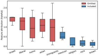
Figure 1: Feature attribution extracted from a fine-tuned BERT model without debiasing for words omitted/included in the manual list used in [14]. The omitted neutral group identifiers actively contributing to the prediction as hateful, which indicates strong biases, are overlooked by human annotators. On the contrary, some less biased words are selected for the debiasing list.

While omitting discriminated group identifiers can undoubtedly strengthen specific biases, over-representation in the debiasing list could also limit model performance through indirect impacts as demonstrated by our experimental results. Moreover, discrimination learned by models is variable to datasets, hyperparameters, and training processes. Hence, exhaustively defining bias through human annotators is unsustainable.

To this end, we proposed a fully automatic misuse detector (MiD), which deploys an explanation method, to identify potentially biased features (tokens/words) at the training stage without any external knowledge or resources. Aiming to perform the detection at runtime, we introduced the false positive proportion FPP as an efficient proxy of feature contributions to predictions since the time complexity of feature attribution examination with the explanation method is impractical. Built upon that, an end-to-end debiasing framework is designed to mitigate bias in hate speech classifiers during the training process. The experimental results show that the list of potentially biased words delivered by the proposed MiD has good coverage on the manually defined list and results in an outstanding performance in balancing accuracy and fairness. Another key finding is that the correction targeting single words has indirect impacts on their semantic neighbors, which calls for more attention to potential effects the debiasing process could bring into hate speech detectors.

The rest of the paper is organized as follows. In Section II, we discuss the related work of machine learning fairness and current progress in explainable AI (XAI), which is an essential component of the proposed framework. Section III details the proposed method MiD for automatic bias detection. Afterwards, the debiasing framework with a staged correction is introduced in Section IV. To evaluate the proposed method, we conduct detailed experiments in Section V. Finally, we discuss and conclude the findings of this work in Section VI.

II Related work

To mitigate discrimination in hate speech classifiers, there are debiasing methods at different stages of the machine learning pipeline proposed. Data augmentation tackles the problem at the data preprocessing stage. Instances relating to under-represented groups are augmented through random combinations of pre-defined templates and group identifiers [36, 16, 7]. But augmentation without supervision always delivers meaningless and unrealistic instances, which could introduce potential risks into the system. Similar to the previous solution, instance weighting balances the distribution of class labels over ethnic groups by editing the weights of entries in the training set [34] during the preprocessing. Without creating synthetic samples, it avoids the potential risks.

Our work is highly related to the recently emerging work which mitigates bias at the training stage. The idea is to debias hate speech classifiers during training by suppressing unwanted model attention on selected neutral words [14]. A static list of group identifiers gives the definition of the sensitive neutral words. Instead of preparing a pre-defined list, [33] suggests correcting model behaviors by involving human-in-the-loop. For both methods, the essential part is the employment of an explanation method, which dominates the derivation of feature attribution.

A feature/word is not necessary to be biased even if it frequently appears in incorrect predictions. Therefore, obtaining insights into the decision making process is the key to the precise treatment for its bias. Recent developments in XAI, especially in explaining text classifiers [5, 20, 4], offer a solution to the detailed analysis by revealing the evidence supporting a decision through explanations. Among different categories, model-agnostic local explanation methods [23, 18] are in favor with debiasing text classifiers, as methods belonging to this category would not harm the flexibility of the debiasing framework since no prerequisites are present for the targeting model, In addition, because state-of-the-art text classifiers treat the same token differently depending on the context [22, 26], we prefer a local explanation method that interprets one decision at a time rather than a global one. Regarding the concrete form of presenting explanations, feature importance [29] outperforms other choices, such as saliency map [28] and counterfactual [21], as it quantifies feature contributions to a prediction, which is accessible to both machine and human.

III Automatic misuse detector

Before introducing the misuse detector, we specify the targeting bias to mitigate in this paper. Imbalanced data distribution is a common problem while solving tasks with data-driven approaches. The same problem also holds for hate speech detection. For example, there are more toxic speeches against specific demographic groups on social media platforms because of social bias and stereotypes. Hate speech detectors trained on these datasets could be biased while observing the high co-occurrence between the group identifiers and the hateful sentiment, which means they may use sensitive identifiers (e.g., “Muslim”, “Jewish”) as evidence for their prediction. This kind of bias is highly undesired and is referred to as “wrong reasons” since it is an obvious misuse of features. Here, we summarize the misuse into two cases:

• Wrong for wrong reasons: a model delivers wrong decisions based on incorrect reasoning of the observations.

• Right for wrong reasons: a model delivers right decisions based on incorrect reasoning of the observations.

Regarding the first case, it is natural that problematic inference produces wrong predictions. However, models could also coincidentally output accurate classification for biased reasons. Detecting misuses in the second case is extremely difficult as we cannot distinguish unreasonable right decisions from the justified ones without external resources. Therefore, we decided to concentrate on bias and misuse that result in wrong decisions as the first step towards automatic bias detection in text classification.

In the following parts of this section, we introduce the proposed automatic misuse detector (MiD). It firstly filters out potentially biased words using an efficient proxy of feature importance (Section III-A, Section III-B) and then conducts a more detailed investigation using an explanation method to finalize the list of discriminated words (Section III-C).

III-A Wrong for wrong reasons

Given a hate speech detector $\mathcal{M}(\cdot)$ and a dataset $\mathcal{D}$ containing input texts $x\in\mathcal{D}$ with each text consisting of a list of tokens (words) in sequential order $x=\{w_{0},w_{1},...,w_{n}\}$, we define a wrong reason for wrong decisions in (1) as a feature $w^{*}$ whose average contribution $\bar{\phi}(w^{*})$ to the misclassified instances is greater than a given threshold $\tau$,

$$\bar{\phi}(w^{*})_{\hat{y}\neq y}=\mathbb{E}_{\hat{y}\neq y}[\phi(w^{*})]>\tau$$ (1)

where $\phi(\cdot)$ denotes the function of deriving feature importance, $\hat{y}$ denotes the prediction on an instance containing the wrong reason $w^{*}$, and $y$ denotes the ground truth of the corresponding instance.

For the sake of simplicity, we here assume the given model $\mathcal{M}$ to be a binary classifier with the output value ranging from 0 to 1, where an output close to $1$ indicates the positive class ($\hat{y}=1$) and vice versa. The contribution of a feature to the prediction can be measured using feature importance score (also known as feature attribution) which is the output of explanation methods. We choose a state-of-the-art explanation method named Sampling and Occlusion (SOC) [12] for our debiasing framework, which defines feature importance as:

$$\phi(w^{*})=\mathbb{E}_{\mathcal{X}_{\delta}}[\mathcal{M}(x)-\mathcal{M}(x\backslash w^{*})]$$

where $\mathcal{X}_{\delta}$ denotes the context of the relevant input $x$. The context consists of the neighboring instances derived from the input $x$ by randomly masking words with padding tokens. The contribution of the feature $w^{*}$ is measured by the expected impact of excluding the target feature from all variants in the given context. With the contribution defined, an intuitive solution for identifying wrong reasons would be finding features whose importance scores are highly correlated to the occurrence of misclassifications. But this is unrealistic at runtime as computations for explaining all inputs are unaffordable. To this end, we propose in the next subsection a loosened proxy of attribution for filtering out the suspicious features, which allows us to conduct the detection in real-time.

It has to be mentioned that other popular explanation methods (e.g., SHAP [18]), which is differentiable, could also be adopted, but SOC is in favor for the efficiency reason. It can concentrate on the filtered out features rather than the whole input and thus helps reduce the computational complexity.

III-B False positive proportion as a proxy of feature attribution

It is more urgent to solve bias that leads to misclassification as hateful than the other way around. Hence, we focus on the false positive instances. But the same theory also applies to the opposite case. For the false positive decision made on the input $x$, a feature which is mainly responsible for the prediction possesses the average importance score $\bar{\phi}(w^{*})_{FP}>\tau$. Although finding words with high attribution values which frequently appear in false positive instances could be an ideal way to determine the potentially misused features, computations carried by explanation methods are usually expensive [24]. It becomes unbearable if such computations have to be carried throughout the whole vocabulary since the size of vocabulary in up-to-date NLP models can easily go up to the order of tens of thousands [6]. Therefore, we use the false positive proportion as an efficient proxy for the detection of the aforementioned wrong reasons supported by the Proposition 1. The false positive proportion of a feature $FPP_{w}$ is defined in (2).

$$\begin{split}FPP_{w}=&~{}\frac{FP_{w}}{FP_{w}+FN_{w}+TP_{w}+TN_{w}}\end{split}$$ (2)

Note that the FPP is slightly different from the false positive rate by definition. It is the ratio of false positive samples among all relevant samples rather than the relevant negatives.

Proposition 1.

For a wrong reason $w^{*}$ where $\phi(w^{*})>\tau$, its false positive proportion satisfies $FPP_{w^{*}}>\tau$.

Proof.

Given a feature $w^{*}$ and the set of false positive instances $FP_{w^{*}}$ possessing the feature $w^{*}$, if $w^{*}$ is responsible for the misclassification, we have:

$$\bar{\phi}(w^{*})_{FP_{w^{*}}}= ~{}\mathbb{E}_{FP_{w^{*}}}[\phi(w^{*})]$$

$$= ~{}\mathbb{E}_{FP_{w^{*}}}[\mathbb{E}_{\mathcal{X}_{\delta}}[\mathcal{M}(x^{\prime})-\mathcal{M}(x^{\prime}\backslash w^{*})]]$$

$$= ~{}\mathbb{E}_{FP_{w^{*}}}[\mathcal{M}(x)-\mathcal{M}(x\backslash w^{*})]$$

$$= ~{}\mathbb{E}_{FP_{w^{*}}}[\mathcal{M}(x)]-\mathbb{E}_{FP_{w^{*}}}[\mathcal{M}(x\backslash w^{*})]>\tau$$

$$\iff ~{}\mathbb{E}_{FP_{w^{*}}}[\mathcal{M}(x)]>\mathbb{E}_{FP_{w^{*}}}[\mathcal{M}(x\backslash w^{*})]+\tau$$

where $x^{\prime}$ indicates an instance from the context $\mathcal{X}_{\delta}$ and $x$ denotes a text that belongs to the set $FP_{w^{*}}$. Here we assume that the average impact of simply masking out $w^{*}$ from all $x\in FP_{w^{*}}$ is equal to the mean of the feature importance, which is derived from the expected impact of excluding $w^{*}$ in the given context $\mathcal{X}_{\delta}$. The greater expected model outcome implies that the given text containing the word $w^{*}$ is more likely to be classified as positive, and thus:

$$\implies ~{}\textbf{Pr}(x\in FP_{w^{*}}|w^{*})>\textbf{Pr}(x\in FP_{w^{*}}|\bar{w}^{*})+\tau$$

$$\iff ~{}\textbf{Pr}(x\in FP_{w^{*}}|w^{*})>\tau$$

$$\iff ~{}\frac{\textbf{Pr}(x\in FP_{w^{*}},w^{*})}{\textbf{Pr}(w^{*})}>\tau$$

$$\iff ~{}\frac{FP_{w^{*}}/|\mathcal{D}|}{(FP_{w^{*}}+FN_{w^{*}}+TP_{w^{*}}+TN_{w^{*}})/|\mathcal{D}|}>\tau$$

$$\iff ~{}FPP_{w^{*}}>\tau$$

where the symbol $\bar{w}^{*}$ indicates that the feature $w^{*}$ is masked out. ∎

For better efficiency of the proxy, we choose another threshold $\eta$ ($\eta\geq\tau$) for the false positive proportion $FPP_{w^{*}}$ as a complement of the neglected term $\textbf{Pr}(x\in FP|\bar{w}^{*})$ on the right side of the inequation during the proof. However, words with FPPs satisfying $FPP_{w}>\eta$ are not directly applicable for the debiasing purpose since the reverse of Proposition 1 does not hold as stated in Proposition 2.

Proposition 2.

For a word $\dot{w}$, the significance of its false positive proportion ($FPP_{\dot{w}}>\tau$) does not imply that it is a considerable reason for the wrong predictions.

Proof.

Given a word $w$ as a wrong reason, if there exists another word $\dot{w}$ which has unconditional high co-occurrence with $w$ (e.g., for semantic/syntactic reasons), it means:

$$\textbf{Pr}(w)=\textbf{Pr}(w,\dot{w})=\textbf{Pr}(\dot{w})$$ (3)

$$\textbf{Pr}(w|x\in FP)=\textbf{Pr}(w,\dot{w}|x\in FP)=\textbf{Pr}(\dot{w}|x\in FP)$$ (4)

The statement about the significant false positive proportion holds for $\dot{w}$ without any constraints on its importance score $\phi(\dot{w})$.

$$\textbf{Pr}(x\in FP|\dot{w})= ~{}\frac{\textbf{Pr}(\dot{w}|x\in FP)}{\textbf{Pr}(\dot{w})}\cdot\textbf{Pr}(x\in FP)$$

$$\overset{\eqref{eq_pr_overall}}{=} ~{}\frac{\textbf{Pr}(\dot{w}|x\in FP)}{\textbf{Pr}(w)}\cdot\textbf{Pr}(x\in FP)$$

$$\overset{\eqref{eq_pr_cond}}{=} ~{}\frac{\textbf{Pr}(w|x\in FP)}{\textbf{Pr}(w)}\cdot\textbf{Pr}(x\in FP)$$

$$= ~{}\textbf{Pr}(x\in FP|w)>\tau$$

$$\iff ~{}FPP_{\dot{w}}>\tau$$

∎

Proposition 2 indicates that the false positive proportion is a loosened proxy of the feature attribution, which requires an in-depth analysis of the identified words to condense the word list before it serves for the debiasing task.

Computation of the FPP can be done in linear time (dependent on the size of the dataset) as model predictions are available during training time. Hence, its computation is much more efficient than exhaustively performing the chosen explanation method for feature attribution. According to Proposition 1, we apply FPP as a proxy to filter out the potentially biased words and then utilize the SOC explainer to exclude features with limited contributions from the final list following Proposition 2. Note that obtaining feature importance is practical after the filtering as the number of words under investigation is about $0.2\%$ of the vocabulary size.

III-C Misuse detection

For the trade-off between accuracy and fairness, we intend to debias a model with minimal external restrictions applied. A model is updating itself for the given task during training. Misconduct of the model at the current step could be self-corrected after finishing further training steps. Accordingly, the misuse detector in the debiasing framework is designed to examine FPPs of features periodically during the training phase instead of completing the detection at once. MiD integrates a sliding window with size $l$ recording the most recent feature statistics. Only features with at least $k$ records in the sliding window, whose FPP exceeds the user-defined threshold $\eta$, namely $FPP_{w}>\eta$, will be added to the candidate list. Fig. 2 demonstrates an example of the candidate list absorbing and rejecting the features according to their FPPs.

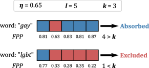
Figure 2: Absorbing and excluding potentially biased features through FPP

Words filtered out by FPP are candidates of debiasing targets. And because of Proposition 2, investigation on their feature importance scores is mandatory. Only candidates with an importance score assigned by SOC greater than the given threshold $\tau$ will be inserted into the debiasing list $W$. The finalized debiasing list $W$ will contribute to the correction of the model.

IV Staged training

Based on MiD proposed in previous subsection, we introduce a staged training process for automatic debiasing in this section. The training process consists of three stages: i) vanilla, ii) correction, and iii) stabilization, which are listed following their orders in the training process. The training process enters the next stage when $n$ training iterations are completed.

At the vanilla stage, no restrictions are applied to the training target. The misuse detector is recording statistics of suspicious features periodically (as entries in the sliding window) in parallel for the construction of the debiasing list $W$. Words inserted into $W$ remain in the list even if their importance scores drop below the threshold $\tau$. The debiasing list $W$ is thus continually growing until the vanilla stage ends. The correction stage follows the end of the vanilla. Misconduct of the model is corrected at this stage with restrictions being applied to the target model based on the debiasing list $W$. To implement the restrictions, the objective function is updated with a regularized explanation term added to the classification objective $\mathcal{L}$ as follows:

$$\mathcal{L}_{E}=\mathcal{L}+\lambda\sum_{w\in W}|\hat{y}-y|\cdot\phi(w)^{2}$$

The second term is the regularization term with the strength controlled by a hyperparameter $\lambda$. Since our focus is solving wrong for wrong reasons, penalties are laid solely on misclassified instances containing features listed in $W$. The debiasing list remains static at this stage regardless of the possible changes of either feature attribution or FPP. After the correction, the debiasing list is resolved. And finally, as the stabilization stage, the model is trained without restrictions for another $n$ steps.

The first two stages are critical in the training process. Unlike the other debiasing methods for text classifiers, which define the debiasing list manually ahead of the training, we first train the target model for $n$ steps and actively search for the discriminated words. It encourages the debiasing framework to be more responsive to the actual model behaviors, which could be affected by trivial changes (e.g., varying random seeds [37]) in the training settings. The variable nature of the training process is another reason why a pre-defined debiasing list should be less favored than maintaining a list at runtime. We apply the extracted knowledge to enforce the correction at the second stage. Though it is not mandatory, the stabilization step is arranged to enable the model to optimize itself but at the risk of reappearing recovered bias.

V Experiments

We designed comprehensive experiments to study the performance of the proposed debiasing framework. Firstly, we analyze the outputs of MiD in a qualitative manner (Section V-B). Secondly, we compare the model which is trained using the staged debiasing framework to its competitors (Section V-C). Last but not least, an investigation to uncover the indirect impacts of debiasing is conducted. And we discuss the overall coverage of MiD on the manual list considering both direct and indirect debiasing impacts (Section V-D). The concrete experimental settings are discussed in the coming Section V-A.

V-A Experiment Details

Dataset: We evaluate our approach on the ”Gab Hate Corpus” [13] dataset. The dataset contains $27,655$ speeches sampled from a social network named ”Gab” which is populated by ”Alt-right” [2] with a high rate of hate speech. There are $22,036$ instances in the training set with $1941$ of them being labeled as hateful ($y=1$) by human annotators and the remaining as non-hateful ($y=0$). The validation set has a size of $2,755$ with $245$ instances as hateful. The test set has the same size as the validation set and includes $264$ positive instances.

Text classifier: The debiasing target is a text classifier solving the hate speech detection task given by the aforementioned dataset. We select BERT [15], a state-of-the-art language model based on the attention mechanism [30], for our experiments. Although BERT has been utilized for numerous downstream tasks, recent researches demonstrate various biases (e.g. gender [3], ethnic [1] bias) it could induce. We fine-tune the pre-trained version that is publicly available in the transformers library [32].

Hyperparameters: For the misuse detector MiD, the two thresholds $\eta$ (for FPP) and $\tau$ (for feature importance score) give the definition of misused terms. A strict definition with high thresholds will lead to the risk of overlooking biases; meanwhile, a detector with low thresholds may involve irrelevant tokens and thus cause damage to the model’s performance. We here determine $\eta$ and $\tau$ via grid search and set them to $0.65$ and $0.45$, respectively. The misuse detector records FPPs of suspicious features every $50$ iteration with the sliding window size $l$ equals $10$ and the requirement of the minimal count $k$ equals $7$. As for the debiasing framework, the strength of the explanation regularization is $0.1$ following the optimal parameter setting in [14]. The training iteration is set to $1,000$ equally for each stage, which indicates $3,000$ training iterations in total.

Competitors: We compare the model corrected by the proposed framework to the two models with the same structure but trained under various circumstances. One is trained under the vanilla setting with no restrictions. The other is trained with the debiasing method proposed in [14], which is considered as a baseline. The baseline employs a manually defined static debiasing list and the strength of the regularization is the same as our method (i.e., $\lambda=0.1$). The static debiasing restrictions take effect during the whole training process, while ours educates the model for fairness only during the middle stage (correction). For both the vanilla setting and the baseline, the models are trained for $3,000$ iterations, which is identical to the total amount of training iterations in the staged correction.

V-B Evaluating misuse detector

We first evaluate the misuse detector as it is the base of the proposed debiasing framework. The list of potentially biased words given by MiD during the first stage is presented in Table I along with the manually selected ones used in the baseline. The words shared by the two lists are marked as bold and summarized in the first row. And for words contained in the manual list, the box plots of the biased feature attribution and the visualization of corresponding FPPs can be found in Fig. 3.

TABLE I: Lists of words for debiasing

Shared by both lists	muslim muslims islam islamic jew jews jewish gay white whites black blacks
Only in MiD	immigrant immigrants left liberal democrats communist african racist nazi leftist corrupt migrants liberals traitor homo rap slave terrorist fucking gender
Only in Manual list	woman women democrat allah lesbian transgender brown race mexican religion homosexual homosexuality africans

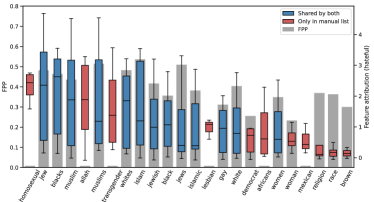
Figure 3: Feature attribution of the manually selected words

The automatically constructed debiasing list covered 12 out of 25 words given in the manual list, which is considered sensitive and potentially discriminated. For example, sensitive group identifiers (such as “muslim”, “black”, and “gay”) are covered by both lists. In addition, MiD successfully identifies words referring to demographic information, like “immigrant” and “liberal”, which are overlooked by the human annotators.

At the same time, we are not surprised that potentially hateful words such as ”nazi” and ”fucking” are also listed. Unreasonably referring to an individual or a group of people as “nazi” is truly hateful and should be filtered out before it gets published in public environments. But the model may ban proper expressions or discussions (e.g., on histories) if it becomes over-sensitive to the potential evidence for hate sentiments. Although the main focus of the work is to mitigate biases carried by hate speech classifiers, over-sensitivity towards potential evidence may also be the wrong reason that is responsible for wrong decisions. It is also a reason why we named the proposed method as misuse detector rather than bias detector.

Furthermore, the box plots of feature attribution in Fig. 3 show that the misuse detector excludes less discriminated words like “race” and “brown”, which exist in the manual list, from the automatic one. Despite the truth that human annotators consider these words discriminated, they play a neutral role (told by the relatively low feature importance scores shown in the box plots) during the decision-making process. In principle, we could include all neutral words in the debiasing list for models’ fairness. But since the experiment in Section V-D demonstrates that attribution suppression on single words would affect their semantic neighbors, we argue that the debiasing list should be concise for model capacities by excluding less biased words.

Apart from the merits, the detector overlooks some manually selected words that are misused, such as “homosexual” and “transgender”. Illustrated by their considerably lower FPPs, the main reason for the incompleteness is that these wrong reasons lead to right predictions. While concentrating on correcting wrong decisions, we selectively neglect the case “right for wrong reasons” as discussed in Section III. Nevertheless, we demonstrate in Section V-D that the debiasing framework lays approving impacts on these words (feature importance scores dropped over $50\%$) even though they are not directly affected.

V-C Evaluating debiasing framework

To reveal the impact of the debiasing framework on training a model, we present in Fig. 4 the training losses under different circumstances.

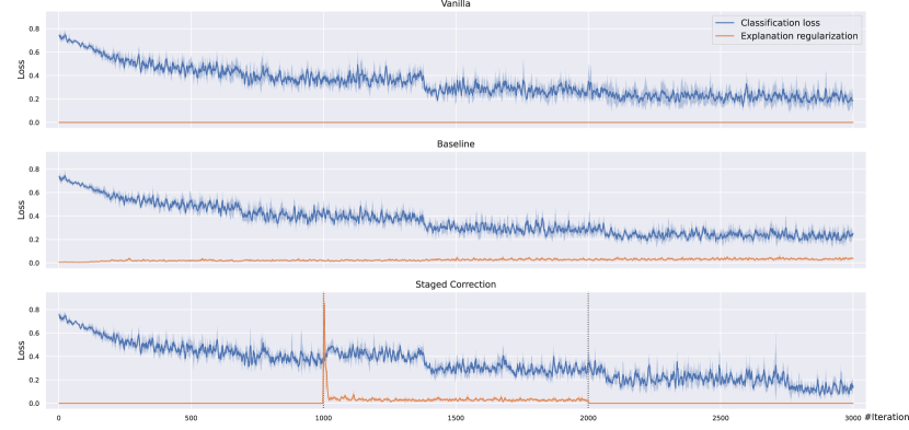
Figure 4: Training loss over iteration with/-out debiasing

Having the lines in blue indicate the pure classification loss (cross-entropy), the orange lines refer to the penalties regularized by explanations, and the sum of the two values is the final back-propagated loss. The model is trained using the same hyperparameters with the only difference in the random seed for 10 times under each setting, and the reported losses are the averaged values of the 10 versions. For the vanilla setting, the penalty introduced by the regularization term is identical to $0$ as no restrictions were applied. And a decreasing trend can be observed for the loss until around the $1,500_{th}$ iteration. The baseline adopted a pre-defined list for debiasing, which remained in force during the whole process. As a consequence of the applied restrictions, the regularization term stays close to $0$, which indicates the extremely low attribution of the debiasing targets. Finally, the loss fluctuates at a level close to the same value under the vanilla setting with a similar progressing period.

As for the staged correction method, we separate the training stages by the vertical dotted line at the $1,000_{th}$ and $2,000_{th}$ iterations. The change of the classification loss is similar to the other two settings at the first stage. The restrictions for debiasing come into effect when the first stage ended. Unlike what is shown in the baseline, the penalty here starts with a very high value at the beginning of the correction stage as certain misbehaviors of the model have been detected by MiD during the first $1,000$ iterations. And the model manages to correct the misuse instantly (less than $100$ iterations) following the guidance of the explanations. At the same time, since the constraints limit the model reasoning its predictions, we observe a notable increase in terms of classification loss. But the model adapts to the changes quickly and starts improving its classification performance again. The restrictions are resolved when the last stage begins, which leads to a further decrease in the classification loss. And surprisingly, the model trained with the staged correction achieved the lowest classification loss among three. A possible cause of the observation is that explanations as guidance for model attribution can improve its performance [35]. Although we do not bring the full expected feature attribution, excluding the irrelevant/wrong features may have a similar effect by reducing the search space.

For a more comprehensive study on the impact of debiasing approaches on the classification task, we also report the performance of the three versions of the same model in Table II. And again, the model is trained $10$ times with various random seeds for each setting, and the averaged performance on the test set followed by the standard deviation is presented. For the staged correction, we store the best performing model on the validation set for each stage separately and then evaluate them with the test set.

TABLE II: Classification performance on the test set

Setting	Acc.	F1	Precision	Recall
Vanilla	87.96 ± 1.22	48.59 ± 1.75	41.47 ± 3.30	59.17 ± 3.13
Baseline	86.85 ± 1.29	44.88 ± 1.26	37.85 ± 2.60	55.83 ± 4.77
MiD-Van.	86.31 ± 0.88	48.45 ± 0.98	38.02 ± 1.68	67.10 ± 3.15
MiD-Cor.	88.93 ± 0.60	47.18 ± 1.51	43.71 ± 2.29	51.73 ± 4.75
MiD-Sta.	89.06 ± 1.42	48.02 ± 1.52	45.08 ± 5.23	52.53 ± 5.36
Accuracy, F1, Precision, Recall (%) are reported on the test set. Van., Cor., and Sta. are the abbreviations of the vanilla, correction, and stabilization stages respectively.

Models from the MiD-Vanilla stage have the lowest averaged accuracy on the test set as it is trained only for $1,000$ iterations. Although they achieve the highest recall in detecting hateful speeches, the obviously low precision indicates that many false positive decisions have been made, which agrees with the high FPPs visualized in Fig. 3. During the correction stage, the biases of the training targets are mitigated, which results in the second highest precision. As a side effect, constraints on the decision making process limit model performance in terms of recall. It also results in an average F1 score that is roughly $1.4\%$ lower than the highest obtained in the vanilla setting. Consistent with the training loss, the final models (at the stabilization stage) delivered by the staged correction reach the highest accuracy among the competitors. In fact, the performance is improved for all listed metrics in comparison with the results of the correction stage. And even though the restrictions have been resolved, the mean precision increases rather than decreases. On the contrary, the baseline, which also debiases the training target by suppressing unwanted attribution, attains a fairly poor performance with all the figures being lower than the vanilla ones. A possible explanation for this observation is that the manually defined debugging list applied during the whole process limits the convergence of the training targets towards the global optimal.

In Fig. 5(a), we show the changes of averaged feature attribution (FA) and averaged false positive proportion FPP over iterations for the words extracted by MiD. For a better comparison between our debiasing framework and the baseline, we visualize the same statistics for the baseline. We want to point out that the words behind the figures are not identical for the two methods as listed in Table I. Records of different training settings are distinguished by color. The solid and dotted lines indicate the averaged FA and FPP of the debiasing targets respectively. A primary observation is the correlation between FA and FPP, especially for the synchronized drop at the beginning of the correction stage and the fluctuation with similar trends since the $1,500_{th}$ iteration. The same observation holds for the plots of the baseline, whose debiasing list has an overlap with the wrong reasons detected by MiD. But finding the correlation in the baseline requires a closer look as the plots are rather flattened. The observed correlation supports our propositions and the usage of FPP as a proxy of feature attribution for identifying wrong reasons for wrong decisions.

The baseline maintained the lower feature attribution for the selected words during the whole process. Suppression of the incorrect reasoning contributes to the low FPP ($\approx 0.1$), which is only one-third of the averaged FPP ($\approx 0.3$) of the same words in a biased model as shown in Fig. 3.

As for the proposed method, the records for the staged correction do not start at the first iteration, because the misuse detector requires time to confirm that the model consistently discriminates against certain features. Corresponding to the massive regularization penalty at the beginning of the correction stage, the averaged feature attribution of the automatically detected words is relatively high before the correction ($\#iter\leq 1,000$) in the proposed debiasing framework. And a sharp decrease of the FA at the start of the correction stage matches the drop of the regularization term reported in the training loss. The feature attribution keeps falling during the correction and becomes competitive at the end of the second stage to the same value in the baseline. Simultaneously, the FPP is experiencing a decrease. After entering the stabilization stage, the FA of the biased words starts recovering because of the release of the restrictions. In spite of the slight increase in the FA, the decline of FPP continues. Starting from an extremely high point of the FPP, our debiasing framework with the staged correction outperforms the baseline in the middle of the correction stage and ends up with the FPP approaching $0$, even though it possesses a larger debiasing list. The loosened restrictions in the staged correction allow the model better explore the solution space and are considered to be the main cause of the better performance compared to the baseline.

V-D Indirect impacts of correction

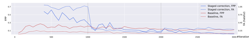
(a) Comparison between the staged correction and the baseline by FA and FPP

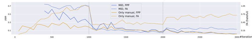
(b) Changes of FA and FPP for words included (“MiD”) and excluded (“Only manual”) in the staged correction

Figure 5: Changes of feature attribution (FA) and false positive proportion (FPP) over iterations

Despite the absence of some manually selected words in the automatically extracted word list, an impressive consistency between the changes of the feature attribution highlights itself in Fig. 5(b). The figure demonstrates the FPP and FA changes for two groups of words in the staged debiasing framework: i) words included in the staged correction process; ii) words omitted by the detector but contained in the manual list. While the debiasing process suppresses the feature attribution of the debiasing targets, the words that are not explicitly included also get affected. Since the experiment is carried on the BERT model, which represents similar tokens with similar embeddings, we believe that correction on single words also brings the effects to their semantic neighbors as they are implicitly connected through semantic meanings.

Motivated by the idea, we conduct further experiments to verify the existence of the indirect impacts. The size of the debiasing list extracted by MiD with the standard parameters is fairly large. To prevent the possible cross effects among multiple features from introducing additional complexity to the analysis, we reduce the number of debiasing targets by raising the two thresholds in MiD to tighten the definition of the wrong reason. By applying the change, the shortened debiasing list (in Table III) contains $6$ words.

TABLE III: Shortened debiasing list

muslims islam jews communist racist homo

In addition to the automatically detected words, from the manual list, we select three words with high cosine similarities to the multiple terms in the previous list, namely “muslim”, “islamic”, and “jewish”. We also choose the two words “homosexuality” and “black” with each having medium similarity to one term and one word “race”, whose embedding is dissimilar to the others. The correlation matrix of the changes in feature attribution and the cosine similarities among word embeddings are presented in Fig. 6. In addition to the listed words

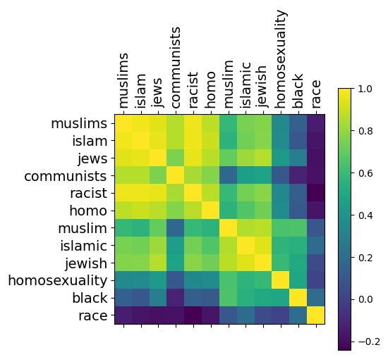
(a) Correlation matrix of FA

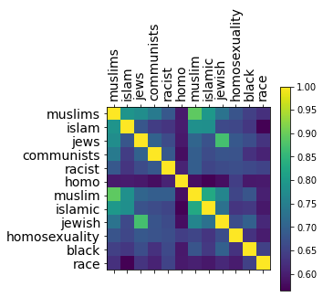
(b) Cosine similarity

Figure 6: Indirect impacts analysis

The bright square at the upper left corner of the correlation matrix in Fig. 6(a) is directly caused by the correction, all the $6$ words relating to the square are actively suppressed by the debiasing framework. And the three words with high similarities to at least two tokens show a strong correlation in terms of feature attribution. For the remaining words, the lower correlations agree with the fact that their embeddings are less similar to the targeting ones. The finding further confirms that suppressing feature attribution of words would indirectly affect their semantic neighbors in a similar way. The more detailed analysis further reveals that overlaying the indirect effects (e.g., indirect effects originating from “muslims” and “islam” on “islamic”) could strengthen the correlation. Considering the semantically similar words shared by both lists in Table I, we, therefore, argue that the proposed misuse detector has better coverage (direct and indirect) on the manual list than it appears to be.

VI Conclusion

In this work, we proposed MiD, a fully automatic misuse detector with the main purpose of uncovering biases learned by a text classifier during the training phase. With the deployment of the detector, the training object is debiased through a staged correction process. Our experiments show the outstanding coverage of the automatically extracted list on the discriminated terms. Based on the dynamically constructed debiasing list, the model trained with the staged correction process achieves similar performance in terms of fairness to the baseline, which applies the strict restrictions for debiasing through the whole training process. Moreover, our debiased model maintains the competitive classification performance in comparison with the biased model trained under no constraints.

We also study the indirect impacts of the word-level correction on the semantically connected words, which are underexplored in previous work. Having the experimental results supporting our assumption about the existence of indirect impacts, we argue that the word list for debiasing should be minimized by excluding less related tokens to avoid introducing unexpected effects to the training target. Additionally, the observation also strengthens the belief that debiasing is a multi-staged task through the NLP pipeline. Bias-free embeddings from the preprocessing stage with sensitive group identifiers distant from sentimental words could reduce the risks of the unintended indirect impacts brought by bias mitigation at the fine-tuning stage into the model capacity.

References

- [1] Jaimeen Ahn and Alice Oh. Mitigating language-dependent ethnic bias in bert. arXiv preprint arXiv:2109.05704, 2021.
- [2] Andrew Anthony. Inside the hate-filled echo chamber of racism and conspiracy theories. The guardian, 18, 2016.
- [3] Rishabh Bhardwaj, Navonil Majumder, and Soujanya Poria. Investigating gender bias in bert. Cognitive Computation, 13(4):1008–1018, 2021.
- [4] Yi Cai, Arthur Zimek, and Eirini Ntoutsi. XPROAX-local explanations for text classification with progressive neighborhood approximation. In 2021 IEEE 8th International Conference on Data Science and Advanced Analytics (DSAA), pages 1–10. IEEE, 2021.
- [5] Hanjie Chen, Guangtao Zheng, and Yangfeng Ji. Generating hierarchical explanations on text classification via feature interaction detection. In Proceedings of the 58th Annual Meeting of the Association for Computational Linguistics, pages 5578–5593, 2020.
- [6] Wenhu Chen, Yu Su, Yilin Shen, Zhiyu Chen, Xifeng Yan, and William Wang. How large a vocabulary does text classification need? a variational approach to vocabulary selection. In Proceedings of NAACL-HLT, pages 3487–3497, 2019.
- [7] Lucas Dixon, John Li, Jeffrey Sorensen, Nithum Thain, and Lucy Vasserman. Measuring and mitigating unintended bias in text classification. In Proceedings of the 2018 AAAI/ACM Conference on AI, Ethics, and Society, pages 67–73, 2018.
- [8] Sahaj Garg, Vincent Perot, Nicole Limtiaco, Ankur Taly, Ed H Chi, and Alex Beutel. Counterfactual fairness in text classification through robustness. In Proceedings of the 2019 AAAI/ACM Conference on AI, Ethics, and Society, pages 219–226, 2019.
- [9] Moritz Hardt, Eric Price, and Nati Srebro. Equality of opportunity in supervised learning. Advances in neural information processing systems, 29, 2016.
- [10] Vasileios Iosifidis, Besnik Fetahu, and Eirini Ntoutsi. FAE: A fairness-aware ensemble framework. In 2019 IEEE International Conference on Big Data (Big Data), pages 1375–1380. IEEE, 2019.
- [11] Vasileios Iosifidis and Eirini Ntoutsi. Adafair: Cumulative fairness adaptive boosting. In Proceedings of the 28th ACM International Conference on Information and Knowledge Management, pages 781–790, 2019.
- [12] Xisen Jin, Zhongyu Wei, Junyi Du, Xiangyang Xue, and Xiang Ren. Towards hierarchical importance attribution: Explaining compositional semantics for neural sequence models. In International Conference on Learning Representations, 2019.
- [13] Brendan Kennedy, et al. The gab hate corpus: A collection of 27k posts annotated for hate speech.
- [14] Brendan Kennedy, Xisen Jin, Aida Mostafazadeh Davani, Morteza Dehghani, and Xiang Ren. Contextualizing hate speech classifiers with post-hoc explanation. In Proceedings of the 58th Annual Meeting of the Association for Computational Linguistics, pages 5435–5442, 2020.
- [15] Jacob Devlin, Ming-Wei Chang Kenton, and Lee Kristina Toutanova. Bert: Pre-training of deep bidirectional transformers for language understanding. In Proceedings of NAACL-HLT, pages 4171–4186, 2019.
- [16] Svetlana Kiritchenko and Saif Mohammad. Examining gender and race bias in two hundred sentiment analysis systems. In Proceedings of the Seventh Joint Conference on Lexical and Computational Semantics, pages 43–53, 2018.
- [17] Qian Li, et al. A survey on text classification: From traditional to deep learning. ACM Transactions on Intelligent Systems and Technology (TIST), 13(2):1–41, 2022.
- [18] Scott M Lundberg and Su-In Lee. A unified approach to interpreting model predictions. Advances in neural information processing systems, 30, 2017.
- [19] Vincent C Müller. Ethics of artificial intelligence and robotics. The Stanford Encyclopedia of Philosophy, 2020.
- [20] W James Murdoch, Peter J Liu, and Bin Yu. Beyond word importance: Contextual decomposition to extract interactions from lstms. In International Conference on Learning Representations, 2018.
- [21] Philip Naumann and Eirini Ntoutsi. Consequence-aware sequential counterfactual generation. In Joint European Conference on Machine Learning and Knowledge Discovery in Databases, pages 682–698. Springer, 2021.
- [22] Matthew E Peters, Waleed Ammar, Chandra Bhagavatula, and Russell Power. Semi-supervised sequence tagging with bidirectional language models. In Proceedings of the 55th Annual Meeting of the Association for Computational Linguistics (Volume 1: Long Papers), pages 1756–1765, 2017.
- [23] Marco Tulio Ribeiro, Sameer Singh, and Carlos Guestrin. ” why should i trust you?” explaining the predictions of any classifier. In Proceedings of the 22nd ACM SIGKDD international conference on knowledge discovery and data mining, pages 1135–1144, 2016.
- [24] Laura Rieger, Chandan Singh, William Murdoch, and Bin Yu. Interpretations are useful: penalizing explanations to align neural networks with prior knowledge. In International conference on machine learning, pages 8116–8126. PMLR, 2020.
- [25] Rachel Rudinger, Jason Naradowsky, Brian Leonard, and Benjamin Van Durme. Gender bias in coreference resolution. In Proceedings of NAACL-HLT, pages 8–14, 2018.
- [26] Justyna Sarzynska-Wawer, et al. Detecting formal thought disorder by deep contextualized word representations. Psychiatry Research, 304:114135, 2021.
- [27] Timo Schick, Sahana Udupa, and Hinrich Schütze. Self-diagnosis and self-debiasing: A proposal for reducing corpus-based bias in nlp. Transactions of the Association for Computational Linguistics, 9:1408–1424, 2021.
- [28] Daniel Smilkov, Nikhil Thorat, Been Kim, Fernanda Viégas, and Martin Wattenberg. Smoothgrad: removing noise by adding noise. arXiv preprint arXiv:1706.03825, 2017.
- [29] Erik Štrumbelj and Igor Kononenko. Explaining prediction models and individual predictions with feature contributions. Knowledge and information systems, 41(3):647–665, 2014.
- [30] Ashish Vaswani, et al. Attention is all you need. Advances in neural information processing systems, 30, 2017.
- [31] Eric Wallace, et al. Allennlp interpret: A framework for explaining predictions of nlp models. In Proceedings of the 2019 Conference on Empirical Methods in Natural Language Processing and the 9th International Joint Conference on Natural Language Processing (EMNLP-IJCNLP): System Demonstrations, pages 7–12, 2019.
- [32] Thomas Wolf, et al. Transformers: State-of-the-art natural language processing In Proceedings of the 2020 conference on empirical methods in natural language processing: system demonstrations, pages 38–45, 2020.
- [33] Huihan Yao, Ying Chen, Qinyuan Ye, Xisen Jin, and Xiang Ren. Refining language models with compositional explanations. Advances in Neural Information Processing Systems, 34, 2021.
- [34] Guanhua Zhang, et al. Demographics should not be the reason of toxicity: Mitigating discrimination in text classifications with instance weighting. In Proceedings of the 58th Annual Meeting of the Association for Computational Linguistics, pages 4134–4145, 2020.
- [35] Zijian Zhang, Koustav Rudra, and Avishek Anand. Explain and predict, and then predict again. In Proceedings of the 14th ACM International Conference on Web Search and Data Mining, pages 418–426, 2021.
- [36] Jieyu Zhao, Tianlu Wang, Mark Yatskar, Vicente Ordonez, and Kai-Wei Chang. Gender bias in coreference resolution: Evaluation and debiasing methods. In Proceedings of the 2018 Conference of the North American Chapter of the Association for Computational Linguistics: Human Language Technologies, volume 2, 2018.
- [37] Donglin Zhuang, Xingyao Zhang, Shuaiwen Song, and Sara Hooker. Randomness in neural network training: Characterizing the impact of tooling. Proceedings of Machine Learning and Systems, 4, 2022.