A Demonstration of Over-the-Air Computation for Federated Edge Learning

Abstract

In this study, we propose a general-purpose synchronization method that allows a set of software-defined radios to transmit or receive any in-phase/quadrature data with precise timings while maintaining the baseband processing in the corresponding companion computers. The proposed method relies on the detection of a synchronization waveform in both receive and transmit directions and controlling the direct-memory access blocks jointly with the processing system. By implementing this synchronization method on a set of low-cost SDRs, we demonstrate the performance of -based , i.e., an over-the-air computation scheme for federated edge learning, and introduce the corresponding procedures. Our experiment shows that the test accuracy can reach more than 95% for homogeneous and heterogeneous data distributions without using channel state information at the edge devices.

I Introduction

over-the-air computation (OAC) leverages the signal-superposition property of wireless multiple-access channels to compute a nomographic function [1]. It has recently gained major attention to reduce the per-round communication latency that linearly increases with the number of edge devices for federated edge learning (FEEL), i.e., an implementation of federated learning (FL) in a wireless network [2, 3]. Despite its merit, an OAC scheme may require the EDs to start their transmissions synchronously with high accuracy [4], which can impose stringent requirements for the underlying mechanisms. In a practical network, time synchronization can be maintained via an external timing reference such as the Global Positioning System (GPS) (see [5] and the references therein), a triggering mechanism as in IEEE 802.11 [6], or well-designed synchronization procedures over random-access and control channels as in cellular networks [7]. However, while using a GPS-based solution can be costly and not suitable for indoor applications, the implementations of a trigger-based synchronization or some synchronization protocols may not be self-sufficient. This is because an entire baseband besides the synchronization blocks may need to be implemented as a hard-coded block to satisfy the timing constraints. On the other hand, when a SDR is used as an I/O peripheral connected to a companion computer (CC) for flexible baseband processing, the transmission/reception instants are subject to a large jitter due to the underlying protocols (e.g., USB, TCP/IP) for the communication between the CC and the SDR. Hence, it is not trivial to use SDRs to test an OAC scheme in practice.

In the state-of-the-art, proof-of-concept OAC demonstrations are particularly in the area of wireless sensor networks. For example, in [8], a statistical OAC is implemented with twenty-one RFID tags to compute the percentages of the activated classes that encode various temperature ranges. A trigger signal is used to achieve time synchronization across the RFIDs. In [9], Goldenbaum and Stańczak’s scheme [10] is implemented with three SDRs emulating eleven sensor nodes and a fusion center. The arithmetic and geometric mean of the sensor readings are computed over a 5 MHz signal. The time synchronization across the sensor nodes is maintained based on a trigger signal and the proposed method is implemented in a field-programmable gate array (FPGA). A calibration procedure is also discussed to ensure amplitude alignment at the fusion center. In [11], the summation is evaluated with a testbed that involves three SDRs as transmitters and an SDR as a receiver. The scheme used in this setup is based on channel inversion. However, the details related to the synchronization are not provided. To the best of our knowledge, an OAC scheme has not been demonstrated in practice for FEEL. In this study, we address this gap and introduce a synchronization method suitable for SDRs. Our contributions are as follows:

Synchronization for CC-based baseband processing: To maintain the time synchronization in an SDR-based network while maintaining the baseband in the CCs, we propose a hard-coded block that is agnostic to the in-phase/quadrature (IQ) data desired to be communicated in the CC. We discuss the corresponding procedures, calibration, and synchronization waveform to address the hardware limitations.

Realization of OAC in practice for FEEL: We realize the proposed method with an intellectual property (IP) core embedded into Adalm Pluto SDR. By using the proposed synchronization method, we demonstrate the performance of -based (FSK-MV) [12, 13, 14], i.e., an OAC scheme for FEEL, for both homogeneous and heterogeneous data distribution scenarios. We also provide the corresponding procedures.

Notation: The complex and real numbers are denoted by $\mathbb{C}$ and $\mathbb{R}$, respectively.

II Proposed Synchronization Method

Consider a scenario where $K$ EDs transmit a set of complex-valued vectors denoted by $\{\textbf{x}_{{\rm UL},k}\in\mathbb{C}^{1\times N_{\rm UL}}|k={1,\hbox to10.00002pt{.\hss.\hss.},K}\}$ to an edge server (ES) in the uplink (UL) in response to the vector $\textbf{x}_{\rm DL}\in\mathbb{C}^{1\times N_{\rm DL}}$ transmitted in the downlink (DL) from the ES, as illustrated in Figure 1LABEL:sub@subfig:systemModel. Assume that the implementation of each ED (and the ES) is based on an SDR where the baseband processing is handled by a CC. Also, due to the communication protocol between the CC and the SDR, consider a large jitter (e.g., in the range of 100 ms) when the IQ data is transferred between the CC and the SDR. Given the large jitter, our goal is to ensure 1) the reception of the vector $\textbf{x}_{\rm DL}$ at the CC of each ED and 2) the reception of the superposed vector $\sum_{k=1}\textbf{x}_{{\rm UL},k}$ (i.e., implying synchronous transmissions for simultaneous reception) at the ES with precise timings (e.g., in the order of $\mu s$) while maintaining the baseband at the CCs.

To address the scenario above, the main strategy that we adopt is to separate any signal processing blocks that maintain the synchronization from the ones that do not need to be implemented under strict timing requirements so that the baseband can still be kept in the CC. Based on this strategy, we propose a hard-coded block that is solely responsible for time synchronization. As shown in 1LABEL:sub@subfig:diagram, the proposed block jointly controls the TX direct-memory access (DMA) and the RX DMA with the processing system (PS) (e.g., Linux on the SDR) as a function of the detection of the synchronization waveform, denoted by $\textbf{x}_{\rm SYNC}$, in the transmit or receive directions through the (active-high) digital signals $e_{\rm tx}[n]\in\{0,1\}$ and $e_{\rm rx}[n]\in\{0,1\}$, respectively. We define two modes for the block:

Mode 1: The default values of $e_{\rm tx}[n]$ and $e_{\rm rx}[n]$ are $0$, i.e., TX DMA and RX DMA cannot transfer the IQ samples. The block listens to the output of the transceiver IP (i.e., the IQ samples in the receive direction), denoted by $x_{\rm rx}[n]$, and constantly searches for the synchronization waveform $\textbf{x}_{\rm SYNC}$. If the vector $\textbf{x}_{\rm SYNC}$ is detected, it sequentially sets $(e_{\rm tx}[n],e_{\rm rx}[n])=(0,1)$ for $T_{\rm RX}$ seconds to allow the RX DMA to move the received IQ samples to the RAM, sets $(e_{\rm tx}[n],e_{\rm rx}[n])=(0,0)$ for $T_{\rm PC}$ seconds, and finally sets $(e_{\rm tx}[n],e_{\rm rx}[n])=(1,0)$ for $T_{\rm TX}$ seconds to allow TX DMA to transfer the IQ samples from the RAM to the transceiver IP.

Mode 2: The default values of $e_{\rm tx}[n]$ and $e_{\rm rx}[n]$ are $1$, i.e., TX DMA and RX DMA can transfer the IQ samples. However, the block listens to the output of the TX DMA (the IQ samples in the transmit direction), denoted by $x_{\rm tx}[n]$. It searches for the vector $\textbf{x}_{\rm SYNC}$. If the vector $\textbf{x}_{\rm SYNC}$ is detected, it blocks the reception by setting $e_{\rm rx}[n]=0$ for $T_{\rm PC}$ seconds.

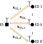
(a) Scenario.

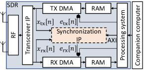
(b) SDR with the proposed synchronization IP.

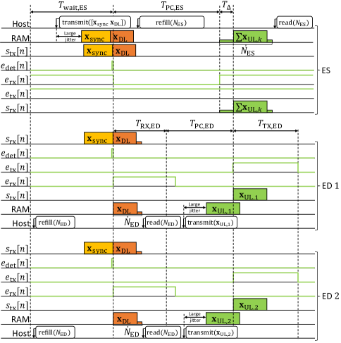
(c) The proposed procedure. While there is a large jitter for any transactions between the RAM and the CC, the proposed block ensures precise timings for the reception of $\textbf{x}_{\rm DL}$ at the EDs, the synchronous transmissions of ${\textbf{x}_{{\rm UL},1}}$ and ${\textbf{x}_{{\rm UL},2}}$ to the ES, and the reception of the superposed signal.

Figure 1: The proposed synchronization block and the corresponding procedure.

Now, assume that the SDRs at the EDs and the ES are equipped with the proposed block and operate at Mode 1 and Mode 2, respectively. We propose the following procedure, illustrated in Figure 1LABEL:sub@subfig:timing, for synchronous communication:

Step 1 (EDs): The CC at each ED executes a command (i.e., $\mathop{\mathrm{refill}}({N_{\rm ED}})$) to fill the RAM with $N_{\rm ED}$ IQ samples in the receive direction for $N_{\rm ED}\geq N_{\rm DL}$. Since RX DMA is disabled by the proposed block at this point, the CC waits for the RX DMA to be enabled by the block.

Step 2 (ES): After the CC at the ES synthesizes the vector $\textbf{x}_{\rm DL}$, it prepends $\textbf{x}_{\rm SYNC}$ to initiate the procedure. It writes $[\textbf{x}_{\rm SYNC}~{}\textbf{x}_{\rm DL}]$ to the RAM and starts TX DMA by executing a command (i.e., $\mathop{\mathrm{transmit}}({[\textbf{x}_{\rm SYNC}~{}\textbf{x}_{\rm DL}]})$). As soon as the block detects the vector $\textbf{x}_{\rm SYNC}$ in the transmit direction, it disables RX-DMA for $T_{\rm PC,ES}$ seconds. Subsequently, the CC issues another command, i.e., $\mathop{\mathrm{refill}}({N_{\rm ES}})$, to fill its RAM in the receive direction, where $N_{\rm ES}$ is the number of IQ samples to be acquired. However, the reception does not start for $T_{\rm PC,ES}$ seconds due to the disabled RX DMA.

Step 3 (EDs): The transceiver IP at each ED receives $[\textbf{x}_{\rm SYNC}~{}\textbf{x}_{\rm DL}]$. As soon as the block detects $\textbf{x}_{\rm SYNC}$, it enables RX DMA. Assuming that $T_{\rm RX,ED}$ is large enough to acquire $N_{\rm ED}$ samples, the RX DMA transfers $N_{\rm ED}$ samples to the RAM as the PS requests for $N_{\rm ED}$ IQ samples on Step 1. The CC reads $N_{\rm ED}$ IQ samples in the RAM via a command, i.e., $\mathop{\mathrm{read}}({N_{\rm ED}})$. As a result, $\textbf{x}_{\rm DL}$ is received with a precise timing.

Step 4 (EDs): The CC at the $k$th ED processes the vector $\textbf{x}_{\rm DL}$ and synthesizes $\textbf{x}_{{\rm UL},k}$ as a response. It then writes $\textbf{x}_{{\rm UL},k}$ to the RAM and initiates TX DMA by executing $\mathop{\mathrm{transmit}}({[\textbf{x}_{\rm SYNC}~{}\textbf{x}_{\rm DL}]})$ before the block enables the TX DMA to transfer. Hence, $\textbf{x}_{{\rm UL},k}$ should be ready in the RAM within $T_{\rm RX,ED}+T_{\rm PC,ED}$ seconds.

Step 5 (EDs): The proposed block at the ED enables the TX-DMA for $T_{\rm TX,ED}$ seconds, where $T_{\rm TX,ED}$ is assumed to be large enough to transmit $N_{\rm UL}$ IQ samples. At this point, the EDs start their transmissions simultaneously.

Step 6 (ES): Assuming that $T_{\rm PC,ES}=T_{\rm RX,ED}+T_{\rm PC,ED}-T_{\Delta}$ and $N_{\rm ES}\geq N_{\rm UL}+\lceil T_{\Delta}/T_{\rm sample}\rceil$, the RX DMA at the ES starts to transfer $N_{\rm ES}$ IQ samples (due to the request in Step 2) $T_{\Delta}$ second before the EDs’ transmissions, where $T_{\rm sample}$ is the sample period. After executing $\mathop{\mathrm{read}}({N_{\rm ES}})$, the ES receives the superposed signal starting from the $\lceil T_{\Delta}/T_{\rm sample}\rceil$ sample.

The procedure can be repeated after the ES waits for $T_{\rm wait,ES}$ seconds to allow the EDs to be ready for the next communication cycle and complete its own internal signal processing, where each cycle takes $T_{\rm PC,ED}+T_{\rm RX,ED}+T_{\rm TX,ED}+T_{\rm wait,ES}$ seconds. Note that the parameters $T_{\rm PC,ED}$, $T_{\rm RX,ED}$, $T_{\rm TX,ED}$, $T_{\rm PC,ES}$, $T_{\Delta}$ and $T_{\rm wait,ES}$ can be pre-configured or configured online by the CC (e.g., through an advanced extensible interface (AXI)). Their values depend on the (slowest) processing speed of the constituent CCs in the network. The timers for $T_{\rm PC,ED}$, $T_{\rm RX,ED}$, $T_{\rm TX,ED}$, and $T_{\rm PC,ES}$ can be implemented as counters that count up on each FPGA clock tick. The distinct feature of the proposed block and the corresponding procedure is that the timers are set up via $\textbf{x}_{\rm SYNC}$ in the receive and transmit directions at both EDs and ES without using the CC.

II-A Synchronization Waveform Design and Its Detection

The design of the synchronization waveform $\textbf{x}_{\rm SYNC}$ and its detection under carrier frequency offset (CFO) with limited FPGA resources were two major issues that we dealt with in our implementation. We address these challenges by synthesizing $\textbf{x}_{\rm SYNC}$ based on a single-carrier (SC) waveform with the roll-off factor of 0.5 by upsampling a repeated binary phase shift keying (BPSK) modulated sequence, i.e., $2[\textbf{g}~{}\textbf{g}~{}\textbf{g}~{}\textbf{g}]-1$, by a factor of $N_{\rm up}=2$ and passing it through a root-raised cosine (RRC) filter, where $\textbf{g}=[g_{1},\hbox to10.00002pt{.\hss.\hss.},g_{32}]\in\mathbb{R}^{1\times 32}$ is a binary Golay sequence. As a result, the null-to-null bandwidth of $\textbf{x}_{\rm SYNC}$ is equal to $0.75f_{\rm sample}$, where $f_{\rm sample}$ is the sample rate.

The rationale behind the design of $\textbf{x}_{\rm SYNC}$ is as follows: 1) An SC waveform with a low-order modulation has a small dynamic range. Hence, it requires less power back-off while it can be represented better after the quantization. 2) A cross-correlation operation can take a large number of FPGA resources due to the multiplications. However, the resulting waveform with the SC waveform with a large roll-off factor is similar to the SC waveform with a rectangular filter. Hence, we can approximately calculate the normalized cross-correlation by using its approximate SC waveform where its samples are either $1$ or $-1$. Hence, the multiplications needed for the cross-correlation can be implemented with additions or subtractions. 3) In practice, $\textbf{x}_{\rm SYNC}$ is distorted due to the CFO. Hence, using a long sequence for cross-correlation can deteriorate the detection performance. To address this issue, we detect the presence of a shorter sequence, i.e., g, back to back four times to declare a detection (i.e., $e_{\rm det}[n]=1$). We choose four repetitions as it provides a good trade-off between overhead and the detection performance. The metric that we use for the detection of g can be expressed as

$$m[n]\triangleq\frac{1}{\lVert\textbf{b}\rVert^{2}}\frac{|\rho[n]|^{2}}{|r[n]|^{2}}=\frac{1}{\lVert\textbf{b}\rVert^{2}}\frac{\langle\textbf{s}_{n},\textbf{b}\rangle^{2}}{\langle\textbf{s}_{n},\textbf{s}_{n}\rangle^{2}}=\frac{\langle\textbf{s}_{n},\textbf{b}\rangle^{2}/2^{12}}{\lVert\textbf{s}_{n}\rVert^{2}}$$ (1)

where b is based on the approximate SC waveform with the rectangular filter and equal to $\textbf{b}=2[g_{32},g_{32},g_{31},g_{31},\hbox to10.00002pt{.\hss.\hss.},g_{1},g_{1}]-1\in\mathbb{R}^{1\times 64}$ for $N_{\rm up}=2$ and $\textbf{s}_{n}$ is $[x_{\rm rx}[n-63],x_{\rm rx}[n-62],\hbox to10.00002pt{.\hss.\hss.},x_{\rm rx}[n]]$ for Mode 1 or $[x_{\rm tx}[n-63],x_{\rm tx}[n-62],\hbox to10.00002pt{.\hss.\hss.},x_{\rm tx}[n]]$ for Mode 2. The block declares a detection if $m[n]$ is larger than 1/4 for four times with 64 samples apart.

II-B Addressing Inaccurate Clocks with Calibration Procedure

The baseband processing (and the additional processing for FEEL) at the ED can take time in the order of seconds. In this case, $T_{\rm PC}$ may need to be set to a large value accordingly. However, using a large value for $T_{\rm PC}$ (also for $T_{\rm RX}$ and $T_{\rm TX}$) results in a surprising time offset problem due to the inaccurate and unstable FPGA clock. To elaborate on this, we model the instantaneous FPGA clock period $T^{{}^{\prime}}_{{\rm clk,}k}[n]$ at the $k$th ED as $T^{{}^{\prime}}_{{\rm clk,}k}[n]=T_{\rm clk}+\Delta T_{{\rm clk},k}+n_{{\rm clk},k}[n]$ where $T_{\rm clk}$ is the ideal clock period and $\Delta T_{{\rm clk},k}$ and $n_{{\rm clk},k}[n]$ are the offset and the jitter due to the imperfect oscillator on the SDR, respectively. The proposed block at the $k$th ED measures $T_{\rm RX,ED}+T_{\rm PC,ED}$ through a counter that counts up till $N_{{\rm cnt}}=(T_{\rm RX,ED}+T_{\rm PC,ED})/{T_{\rm clk}}$ with the FPGA clock ticks. Therefore, the difference between $T_{\rm RX,ED}+T_{\rm PC,ED}$ and the measured one can be calculated as

$$\Delta T_{k}=T_{\rm PC}-\sum_{n=0}^{N_{{\rm cnt}}-1}T^{{}^{\prime}}_{{\rm clk,}k}[n]={N_{{\rm cnt}}\Delta T_{{\rm clk},k}}+{\sum_{n=0}^{N_{{\rm cnt}}-1}n_{{\rm clk},k}[n]}~{},$$

which implies that a large $N_{{\rm cnt}}$ causes not only a large time offset (the first term) but also a large jitter (second term). The jitter can be mitigated by reducing $N_{{\rm cnt}}$ or using a more stable oscillator in the SDR. To address the time offset, we propose a closed-loop calibration procedure as illustrated in Figure 2. In this method, the ES transmits a trigger signal, denoted by ${\textbf{t}_{\rm cal}}$, along with $\textbf{x}_{\rm SYNC}$ as shown in Figure 2LABEL:sub@subfig:calTrigger. After the $k$th ED receives ${\textbf{t}_{\rm cal}}$, it responds to the trigger signal with a calibration signal, denoted by $\textbf{x}_{{\rm cal},k}$, $\forall k$, such that the received calibration signals are desired to be aligned back to back. With cross-correlations, the ES calculates $\Delta T_{k}$, $\forall k$. It then transmits a feedback signal denoted by ${\textbf{t}_{\rm feed}}$ as in Figure 2LABEL:sub@subfig:calFeedback, where ${\textbf{t}_{\rm feed}}$ contains time offset information for all EDs, i.e., $\{\Delta T_{k},\forall k\}$. Subsequently, each ED updates its local $T_{\rm PC,ED}$ as $T_{\rm PC,ED}+\Delta T_{k}$. In this study, we construct ${\textbf{t}_{\rm cal}}$ based on a custom design, detailed in Section IV, while the calibration signals are based on Zadoff-Chu (ZC) sequences.

It is worth noting that the feedback signal may be generalized to include information related received signal power, transmit power increment, or CFO. In this study, the feedback signal also contains transmit power offset and CFO for each ED so that a coarse power alignment and frequency synchronization can be maintained within the capabilities of the SDRs.

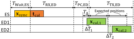
(a) Calibration trigger.

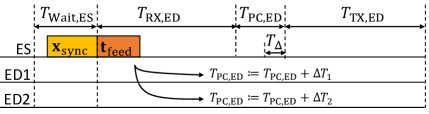
(b) Calibration feedback.

Figure 2: The proposed procedure for calibration.

III Proposed OAC Procedure for FEEL

In this study, we implement FEEL based on the OAC scheme, i.e., FSK-MV, originally proposed in [12] and extended in [14] with the absentee votes. To make the reader familiar with this scheme, let $\mathcal{D}_{k}$ denote the local data set containing the labeled data samples $({\textrm{{x}}}_{{\ell}},{y}_{{\ell}})$ at the $k$th ED for $k=1,\hbox to10.00002pt{.\hss.\hss.},K$, where ${\textrm{{x}}}_{{\ell}}$ and ${y}_{{\ell}}$ are ${\ell}$th data sample and its associated label, respectively. The main problem tackled with FEEL can be expressed as

$${\textbf{w}^{*}}=\arg\min_{\textbf{w}}F(\textbf{w})=\arg\min_{\textbf{w}}\frac{1}{|\mathcal{D}|}\sum_{\forall({\textrm{{x}}},{y})\in\mathcal{D}}f(\textbf{w},{\textrm{{x}}},{y})~{},$$ (2)

where $\mathcal{D}=\mathcal{D}_{1}\cup\cdots\cup\mathcal{D}_{K}$ and $f(\textbf{w},{\textrm{{x}}},{y})$ is the sample loss function measuring the labeling error for $({\textrm{{x}}},{y})$ for the parameter vector $\textbf{w}=[{w}_{1},\hbox to10.00002pt{.\hss.\hss.},{w}_{Q}]^{\rm T}\in\mathbb{R}^{Q}$.

To solve (2) in a wireless network with OAC in a distributed manner (i.e., the global data set $\mathcal{D}$ cannot be formed by uploading the local data sets to the ES), for the $n$th parameter-update round, the $k$th ED first calculates the local stochastic gradients as

$$\tilde{\textbf{g}}_{k}^{(n)}=\nabla F_{k}(\textbf{w}^{(n)})=\frac{1}{n_{\rm b}}\sum_{\forall({\textrm{{x}}}_{{\ell}},{y}_{{\ell}})\in\mathcal{\tilde{D}}_{k}}\nabla f(\textbf{w}^{(n)},{\textrm{{x}}}_{{\ell}},{y}_{{\ell}})~{},$$ (3)

where $\tilde{\textbf{g}}_{k}^{(n)}=[{\tilde{g}}_{k,1}^{(n)},\hbox to10.00002pt{.\hss.\hss.},{\tilde{g}}_{k,Q}^{(n)}]$ is the gradient vector, $\mathcal{\tilde{D}}_{k}\subset\mathcal{D}_{k}$ is the selected data batch from the local data set and $n_{\rm b}=|\mathcal{\tilde{D}}_{k}|$ as the batch size. Similar to the distributed training strategy by the MV with sign stochastic gradient descent (signSGD) [15], each ED then activates one of the two subcarriers determined by the time-frequency index pairs $(m^{+},l^{+})$ and $(m^{-},l^{-})$ for $m^{+},m^{-}\in\{0,1,\hbox to10.00002pt{.\hss.\hss.},S-1\}$ and $l^{+},l^{-}\in\{0,1,\hbox to10.00002pt{.\hss.\hss.},M-1\}$ with the symbols $t_{k,{l^{+}},{m^{+}}}^{(n)}$ and $t_{k,{l^{-}},{m^{-}}}^{(n)}$, $\forall q$ as

$$t_{k,{l^{+}},{m^{+}}}^{(n)}=\sqrt{E_{\rm s}}s_{k,q}^{(n)}\omega{\left({\tilde{g}}_{k,q}^{(n)}\right)}\mathbb{I}\left[{\operatorname{sign}({\tilde{g}}_{k,q}^{(n)})=1}\right]~{},$$ (4)

and

$$t_{k,{l^{-}},{m^{-}}}^{(n)}=\sqrt{E_{\rm s}}s_{k,q}^{(n)}\omega{\left({\tilde{g}}_{k,q}^{(n)}\right)}\mathbb{I}\left[{\operatorname{sign}({\tilde{g}}_{k,q}^{(n)})=-1}\right]~{},$$ (5)

respectively, where $\omega{\left({\tilde{g}}_{k,q}^{(n)}\right)}=1$ for $|{\tilde{g}}_{k,q}^{(n)}|\geq\mathscr{t}$, otherwise it is $0$, $E_{\rm s}=2$ is the normalization factor, $s_{k,q}^{(n)}$ is a random quadrature phase-shift keying (QPSK) symbol to reduce the peak-to-mean envelope power ratio (PMEPR), the function $\operatorname{sign}\left(\cdot\right)$ results in $1$, $-1$, or $\pm 1$ at random for a positive, a negative, or a zero-valued argument, respectively, and the function $\mathbb{I}\left[{\cdot}\right]$ results in $1$ if its argument holds, otherwise it is $0$. The $K$ EDs then access the wireless channel on the same time-frequency resources simultaneously with $S$ OFDM symbols consisting of $M$ active subcarriers. In [14], it is shown that $\mathscr{t}>0$ (i.e., enabling absentee votes) can improve the test accuracy by eliminating the converging EDs from the MV calculation when the data distribution is heterogeneous.

Let $r_{{l^{+}},{m^{+}}}^{(n)}$ and $r_{{l^{-}},{m^{-}}}^{(n)}$ be the received symbols after the superposition for the $q$th gradient at the ES. The ES detects the MV for the $q$th gradient with an energy detector as

$${v}^{(n)}_{q}=\operatorname{sign}\left({\Delta}^{(n)}_{q}\right)~{},$$ (6)

where ${\Delta}^{(n)}_{q}\triangleq{e_{q}^{+}-e_{q}^{-}}$ for $e_{q}^{+}\triangleq|r_{{l^{+}},{m^{+}}}^{(n)}|_{2}^{2}$ and $e_{q}^{-}\triangleq|r_{{l^{+}},{m^{+}}}^{(n)}|_{2}^{2}$, $\forall q$. Finally, the ES transmits $\textbf{v}^{(n)}=[{v}^{(n)}_{1},\hbox to10.00002pt{.\hss.\hss.},{v}^{(n)}_{Q}]^{\rm T}$ to the EDs and the models at the EDs are updated as $\textbf{w}^{(n+1)}=\textbf{w}^{(n)}-\eta\textbf{v}^{(n)}$, where $\eta$ is the learning rate.

In [12] and [14], the reception of the MV vector by the EDs is assumed to be perfect. In practice, the MVs can be communicated via traditional communication methods. Nevertheless, as it increases the complexity of the EDs, we also use the FSK in the DL in our implementation as done for the UL.

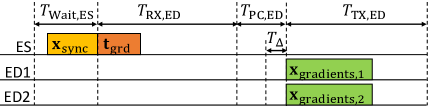
(a) Gradient trigger.

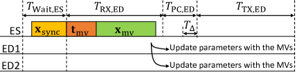
(b) MV feedback.

Figure 3: The proposed procedure for OAC with FSK-MV.

In Figure 3, we illustrate the proposed procedure for FSK-MV. Assuming that the calibration is done via the procedure in Section II-B, the ES initiates the OAC by transmitting a trigger signal, i.e., ${\textbf{t}_{\rm grd}}$, along with the synchronization waveform. The $k$th EDs responds to the received ${\textbf{t}_{\rm grd}}$ with $\textbf{x}_{{\rm gradients},k}$, $\forall k$, i.e., the IQ samples calculated based on (4) and (5). After the ES receives the superposed modulation symbols, it calculates the MVs with (6), $\forall q$. Afterwards, it synthesizes the IQ samples consisting the OFDM symbols based on FSK, i.e., $\textbf{x}_{{\rm mv}}$ and transmits $\textbf{x}_{{\rm mv}}$ along with ${\textbf{t}_{\rm mv}}$ as shown in Figure 3LABEL:sub@subfig:MVfeed. Each ED decodes ${\textbf{t}_{\rm mv}}$ to detect the following samples include the MVs. After decoding the received $\textbf{x}_{{\rm mv}}$, each ED updates its model parameters. Similar to ${\textbf{t}_{\rm cal}}$ and ${\textbf{t}_{\rm feed}}$, the signals ${\textbf{t}_{\rm grd}}$ and ${\textbf{t}_{\rm mv}}$ are based on the physical layer protocol data unit (PPDU) discussed in Section IV. Over all procedure including the calibration phase within one communication round is illustrated in Figure 4.

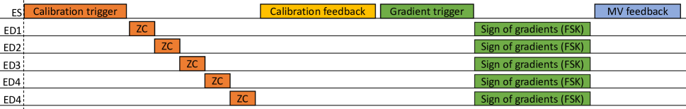
Figure 4: The procedure for FSK-MV along with calibration phase. With the calibration feedback, power offset, CFO, and time offset are fed back to each ED.

IV Proposed PPDU for Signaling

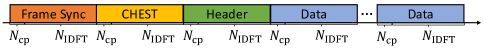
Figure 5: The structure of the proposed PPDU for ${\textbf{t}_{\rm cal}}$, ${\textbf{t}_{\rm feed}}$, ${\textbf{t}_{\rm grd}}$, ${\textbf{t}_{\rm mv}}$

The signaling between EDs and ES in this study is maintained over a custom PPDU as shown in Figure 5, and the signaling occurs through the bits transmitted over the PPDU. In this design, there are four different fields, i.e., frame synchronization, channel estimation (CHEST), header, and data fields, where each field is based on OFDM symbols. We express an OFDM symbol as

$$\textbf{{t}}=\textbf{{A}}\textbf{{F}}_{N_{\rm IDFT}}^{\rm H}\textbf{{M}}_{\textrm{f}}\textbf{{d}}~{},$$ (7)

where $\textbf{{A}}\in\mathbb{R}^{N_{\rm IDFT}+N_{\rm cp}\times N_{\rm IDFT}}$ is the cyclic prefix (CP) addition matrix, $\textbf{{F}}_{N_{\rm IDFT}}^{\rm H}\in\mathbb{C}^{N_{\rm IDFT}\times N_{\rm IDFT}}$ is the normalized $N_{\rm IDFT}$-point inverse DFT (IDFT) matrix (i.e., $\textbf{{F}}_{N_{\rm IDFT}}^{\rm H}\textbf{{F}}_{N_{\rm IDFT}}={\textbf{{I}}_{N_{\rm IDFT}}}$), $\textbf{{M}}_{\textrm{f}}\in\mathbb{R}^{N_{\rm IDFT}\times M}$ is the mapping matrix that maps the modulation symbols to the subcarriers, and $\textbf{{d}}\in\mathbb{C}^{M\times 1}$ contains the modulation symbols on $M$ subcarriers. For all fields, we set the IDFT size and the CP size as $N_{\rm IDFT}=256$ and $N_{\rm cp}=64$, respectively. For CHEST, header, and data fields, we use $M=192$ active subcarriers along with 8 direct current (DC) subcarriers. For the frame synchronization field, the DC subcarriers are also utilized.

IV-A Frame synchronization field

The frame synchronization field is a single OFDM symbol. Every other active subcarrier within the band is utilized with a ZC sequence of length $97$. Therefore, the corresponding OFDM symbols has two repetitions in the time domain. While the repetitions are used to estimate the CFO at the receiver, the null subcarriers are utilized to estimate the noise variance.

IV-B CHEST field

The CHEST field is a single OFDM symbol. The modulation symbols are the elements of a pair of QPSK Golay sequences of length $96$, denoted by $(\textbf{g}_{\rm a},\textbf{g}_{\rm b})$. The vector d is constructed by concatenating $\textbf{g}_{\rm a}$ and $\textbf{g}_{\rm b}$.

IV-C Header field

The header is a single OFDM symbol. It is based on BPSK symbols with a polar code of length $128$ with the rate of $1/2$. We reserve 56 bits for a sequence of signature bits, the number of codewords in the data field, i.e., $N_{\rm cw}$, and the number of pre-padding bits, i.e., $N_{\rm pad}$. The rest of the $8$ bits are reserved for cyclic redundancy check (CRC). We also use QPSK-based phase tracking symbols for every other two subcarriers, where the tracking symbols are the elements of a QPSK Golay sequence of length $64$.

IV-D Data field

Let $N_{\rm bit}$ be the number of information bits to be communicated. We calculate the number of codewords and the number of pre-padding bits as $N_{\rm cw}=\lceil N_{\rm bit}/56\rceil$ and $N_{\rm pad}=56N_{\rm cw}-N_{\rm bit}$. After the information bits are padded with $N_{\rm pad}$, they are grouped into $N_{\rm cw}$ messages of length 56 bits. The concentration of each message sequence and its corresponding CRC is encoded with a polar code of length $128$ with the rate of $1/2$. We carry one codeword on each OFDM symbol with BPSK modulation. Hence, the number of OFDM symbols in the data field is also $N_{\rm cw}$. Similar to the header, QPSK-based phase tracking symbols are used for every other two subcarriers.

IV-E Signaling

Throughout this study, we use the information bits that are transmitted over the PPDU to signal ${\textbf{t}_{\rm cal}}$, ${\textbf{t}_{\rm feed}}$, ${\textbf{t}_{\rm grd}}$, ${\textbf{t}_{\rm mv}}$ and user multiplexing. We dedicate $4$ bits for signaling type and $25$ bits for user multiplexing. If the signaling type is the calibration feedback, we define 32 bits for time offset and 8 bits for power control for each ED.

V Experiment

For the experiment, we consider the learning task of handwritten-digit recognition with $K=5$ EDs and ES, where each of them is implemented with Adalm Pluto (Rev. C) SDRs. We develop the IP core for the proposed synchronization method by using MATLAB HDL Coder and embed it to the FPGA (Xilinx Zynq XC7Z010) based on the guidelines provided in [16]. As shown in Figure 6, we use a Microsoft Surface Pro 4 for the EDs, where an independent thread runs for each ED. The CC for the ES is an NVIDIA Jetson Nano development module. The baseband and machine learning algorithms are written in the Python language. We run the experiment in an indoor environment where the mobility is relatively low. The link distance between an ED and the ES is approximately 5 m. The sample rate is $f_{\rm sample}=20$ Msps for all radios and the signal bandwidth is approximately $15$ MHz. We synthesize the vectors ${\textbf{t}_{\rm cal}}$, ${\textbf{t}_{\rm feed}}$, ${\textbf{t}_{\rm grd}}$, ${\textbf{t}_{\rm mv}}$ based on the custom PPDU discussed in Section IV and consider the same OFDM symbol structure in the PPDU for $\textbf{x}_{{\rm mv}}$ $\textbf{x}_{{\rm gradients},k}$, and $\textbf{x}_{{\rm cal},k}$, $\forall k$. For the synchronization IP, the pre-configured values of $T_{\rm wait,ES}$, $T_{\rm PC,ED}$, $T_{\rm RX,ED}$, $T_{\rm TX,ED}$, and $T_{\Delta}$ are $750$ ms, $750$ ms, $50$ ms, $50$ ms, and $100~{}\mu$s, respectively.

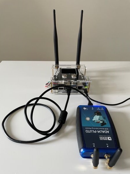
(a) The ES with an NVIDIA Jetson Nano.

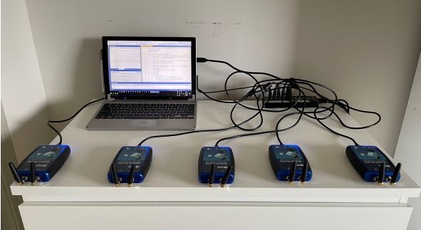
(b) The EDs with Microsoft Surface Pro 4. An independent thread runs for each SDR.

Figure 6: The implemented EDs and ES with an NVIDIA Jetson Nano, a Microsoft Surface Pro 4, and 6 Analog Device Adalm Pluto SDRs for FEEL.

We use the MNIST database that contains labeled handwritten-digit images. To prepare the data, we first choose $|\mathcal{D}|=25000$ training images from the database, where each digit has distinct $2500$ images. For homogeneous data distribution, each ED has $500$ distinct images for each digit. For heterogeneous data distribution, $k$th ED has the data samples with the labels $\{k-1,k,1+k,2+k,3+k,4+k\}$. For both distributions, the EDs do not have common training images. For the model, we consider a convolution neural network (CNN) that consists of two 2D convolutional layers with the kernel size $[5,5]$, stride $[1,1]$, and padding $[2,2]$, where the former layer has $1$ input and $16$ output channels and the latter one has $16$ input and $32$ output channels. Each layer is followed by batch norm, rectified linear units, and max pooling layer with the kernel size 2. Finally, we use a fully-connected layer followed by softmax. Our model has $Q=29034$ learnable parameters that result in $S=303$ OFDM symbols for FSK-MV. We set $\eta=0.001$ and $n_{\rm b}=100$. For the test accuracy, we use $10000$ test samples in the database.

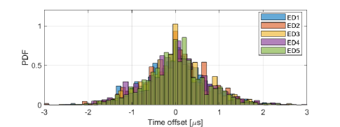
Figure 7: The distribution of time synchronization error due to the imperfect clocks in Adalm Pluto SDRs.

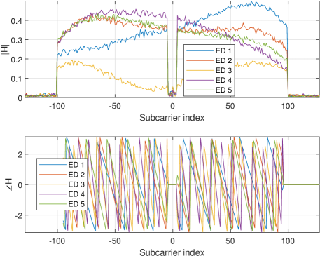
Figure 8: An instant of channel frequency response during the experiment.

The experiment reveals many practical issues. The FPGA clock rate of Adalm Pluto SDR is 100 MHz, generated from a 40 MHz oscillator where the frequency deviation is rated at 20 PPM. Due to the large deviation and $T_{\rm PC,ED}+T_{\rm RX,ED}$, we observe a large time offset and a large jitter as discussed in Section II-B. Hence, the ES initiates the calibration procedure in Figure 2 after completing the OAC procedure in Figure 3, sequentially. In Figure 7, we provide the distribution of the jitter after the calibration, where the standard deviation of the jitter is around $1~{}\mu$s for $T_{\rm PC,ED}+T_{\rm RX,ED}=0.8$ s. Although the jitter can be considerably large, we conduct the experiment under this impairment to demonstrate the robustness of FSK-MV against synchronization errors. In the experiment, a line-of-sight path is present. Nevertheless, the channel between an ED and the ES is still frequency selective as can be seen in Figure 8. In the experiment, we observe that the magnitudes of the channel frequency coefficients do not change significantly due to the low mobility. However, their phases change in an intractable manner due to the random time offsets. Nevertheless, this is not an issue for FSK-MV as it does not require a phase alignment. Note that we also implement a closed-loop power control by using the calibration procedure to align the received signal powers. However, an ideal power alignment is challenging to maintain. For example, ED 3’s channel in Figure 8 is relatively under a deep fade, but the SDR’s transmit power cannot be increased further. Similar to the jitter, we run the experiment under non-ideal power control.

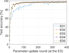
(a) Homegenous, wo. absentee votes.

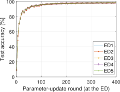
(b) Homegenous, w. absentee votes.

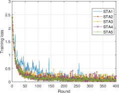
(c) Homegenous, wo. absentee votes.

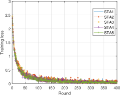
(d) Homegenous, w. absentee votes.

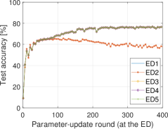
(e) Heterogeneous, wo. absentee votes.

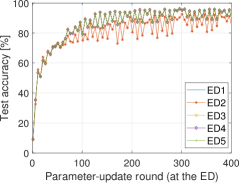
(f) Heterogeneous, w. absentee votes.

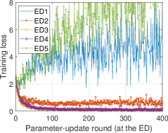
(g) Heterogeneous, wo. absentee votes.

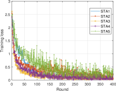
(h) Heterogeneous, w. absentee votes.

Figure 9: Experiment results for the FEEL with the OAC scheme FSK-MV with/without absentee votes.

Finally, in Figure 9, we provide the test accuracy and training loss at each ED when the training is done without absentee votes ($\mathscr{t}=0$) and with absentee votes ($\mathscr{t}=0.005$). For homogeneous data distribution, the test accuracy for each ED quickly reaches 97.5% for both cases as given in Figure 9LABEL:sub@subfig:acc_hete0_abs0 and Figure 9LABEL:sub@subfig:acc_hete0_abs1. The corresponding training losses also decrease as shown in Figure 9LABEL:sub@subfig:loss_hete0_abs0 and Figure 9LABEL:sub@subfig:loss_hete0_abs1. For heterogeneous data distribution scenario, eliminating converging ED improves the test accuracy considerably. For example, in Figure 9LABEL:sub@subfig:loss_hete1_abs0, the training losses for ED 1 and ED 5 gradually increase, which indicates that the digit $0$ and the digit $9$ cannot be learned well since these images are available at ED 1 and ED 5. Therefore, the test accuracy drops below 80% as shown in Figure 9LABEL:sub@subfig:acc_hete1_abs0. However, with absentee votes, this issue is largely addressed and test accuracy reaches 95% as can be seen in Figure 9LABEL:sub@subfig:acc_hete1_abs1.

VI Conclusion

In this study, we propose a method that can maintain the synchronization in an SDR-based network without implementing the baseband as a hard-coded block. We also provide the corresponding procedure and discuss the design of the synchronization waveform to address the hardware limitations. Finally, by implementing the proposed concept with Adalm Pluto SDRs, for the first time, we demonstrate the performance of an OAC, i.e., FSK-MV, for FEEL. Our experiment shows that FSK-MV provides robustness against time synchronization errors and can result in a high test accuracy in practice.

References

- [1] M. Goldenbaum, H. Boche, and S. Stańczak, “Nomographic functions: Efficient computation in clustered gaussian sensor networks,” IEEE Trans. Wireless Commun., vol. 14, no. 4, pp. 2093–2105, 2015.
- [2] G. Zhu, Y. Du, D. Gündüz, and K. Huang, “One-bit over-the-air aggregation for communication-efficient federated edge learning: Design and convergence analysis,” IEEE Trans. Wireless Commun., vol. 20, no. 3, pp. 2120–2135, Nov. 2021.
- [3] P. Liu, J. Jiang, G. Zhu, L. Cheng, W. Jiang, W. Luo, Y. Du, and Z. Wang, “Training time minimization for federated edge learning with optimized gradient quantization and bandwidth allocation,” Front Inform Technol Electron Eng, vol. 23, no. 8, pp. 1247–1263, 2022.
- [4] U. Altun, G. K. Kurt, and E. Ozdemir, “The magic of superposition: A survey on simultaneous transmission based wireless systems,” 2021. [Online]. Available: https://arxiv.org/abs/2102.13144
- [5] K. Alemdar, D. Varshney, S. Mohanti, U. Muncuk, and K. Chowdhury, “RFClock: Timing, phase and frequency synchronization for distributed wireless networks,” in Proc. International Conference on Mobile Computing and Networking (MobiCom), 2021, p. 15–27.
- [6] B. Bellalta and K. Kosek-Szott, “AP-initiated multi-user transmissions in IEEE 802.11ax WLANs,” Ad Hoc Networks, vol. 85, pp. 145–159, 2019.
- [7] E. Dahlman, S. Parkvall, and J. Skold, 5G NR: The Next Generation Wireless Access Technology, 1st ed. USA: Academic Press, Inc., 2018.
- [8] P. Jakimovski, F. Becker, S. Sigg, H. R. Schmidtke, and M. Beigl, “Collective communication for dense sensing environments,” in Proc. IEEE Intelligent Environments, 2011, pp. 157–164.
- [9] A. Kortke, M. Goldenbaum, and S. Stańczak, “Analog computation over the wireless channel: A proof of concept,” in Proc. IEEE Sensors, 2014, pp. 1224–1227.
- [10] M. Goldenbaum and S. Stanczak, “Robust analog function computation via wireless multiple-access channels,” IEEE Trans. Commun., vol. 61, no. 9, pp. 3863–3877, 2013.
- [11] U. Altun, S. T. Başaran, H. Alakoca, and G. K. Kurt, “A testbed based verification of joint communication and computation systems,” in Proc. IEEE Telecommunication Forum (TELFOR), 2017, pp. 1–4.
- [12] A. Şahin, B. Everette, and S. Hoque, “Distributed learning over a wireless network with FSK-based majority vote,” in Proc. IEEEE International Conference on Advanced Communication Technologies and Networking (CommNet), Dec. 2021, pp. 1–9.
- [13] M. H. Adeli and A. Şahin, “Multi-cell non-coherent over-the-air computation for federated edge learning,” in Proc. IEEE International Conference on Communications (ICC), Apr. 2022, pp. 1–6.
- [14] A. Şahin, “Distributed learning over a wireless network with non-coherent majority vote computation,” 2022. [Online]. Available: https://arxiv.org/abs/2209.04692
- [15] J. Bernstein, Y.-X. Wang, K. Azizzadenesheli, and A. Anandkumar, “signSGD: Compressed optimisation for non-convex problems,” in Proc. in International Conference on Machine Learning, vol. 80. Proceedings of Machine Learning Research, 10–15 Jul 2018, pp. 560–569.
- [16] Analog Device, “plutosdr-fw, v34,” 2022. [Online]. Available: https://github.com/analogdevicesinc/plutosdr-fw.git