Contextuality as a precondition for entanglement

Abstract

Quantum theory features several phenomena which can be considered as resources for information processing tasks. Some of these effects, such as entanglement, arise in a non-local scenario, where a quantum state is distributed between different parties. Other phenomena, such as contextuality can be observed, if quantum states are prepared and then subjected to sequences of measurements. Here we provide an intimate connection between different resources by proving that entanglement in a non-local scenario can only arise if there is preparation & measurement contextuality in a sequential scenario derived from the non-local one by remote state preparation. Moreover, the robust absence of entanglement implies the absence of contextuality. As a direct consequence, our result allows to translate any inequality for testing preparation & measurement contextuality into an entanglement test; in addition, entanglement witnesses can be used to obtain novel contextuality inequalities.

Introduction

Quantum information science bears the promise to lead to novel ways of information processing, which are superior to classical methods. This begs the question, which quantum phenomena are responsible for the quantum advantage and which resources are needed to overcome classical limits. There are two main scenarios where genuine quantum effects are studied. First, in the nonlocal scenario (NLS), two parties, Alice and Bob, share a bipartite quantum state $\rho_{AB}$ and perform different measurements on it. This leads to a joint probability distribution for the possible outcomes. Second, in the sequential scenario (SQS), Alice prepares some quantum state $\sigma$, transmits the quantum state to Bob which performs a measurement. Clearly, these scenarios are connected: In the NLS Alice and Bob can, using classical communication, postselect on the outcome of Alice’s measurement, so that Alice remotely prepares the state $\sigma$ for Bob, see also Fig. 1.

In both scenarios, several notions of classicality are known and have been identified as resources for special tasks. For the NLS a major example is entanglement which arises if the quantum state cannot be generated by local operations and classical communication [1, 2]. Entanglement has been identified as a resource for tasks like quantum key distribution [3] or quantum metrology [4, 5]. Other examples of non-classicality in the NLS are quantum steering and [6] and Bell nonlocality [7].

For the SQS a major notion of non-classicality is based on quantum contextuality [8, 9]. For preparation noncontextuality one asks whether there is a hidden variable (HV) model for Alice’s preparations obeying some assumptions, while measurement noncontextuality refers to the same question for Bob’s measurements. Often, the underlying notions of classicality are combined to preperation and measurement (P&M) contextuality, sometimes also called simplex embeddability [10, 11, 12, 13]. Effects of contextuality can be viewed as resources in various tasks, such as quantum state discrimination [14] and parity-oblivious multiplexing [15].

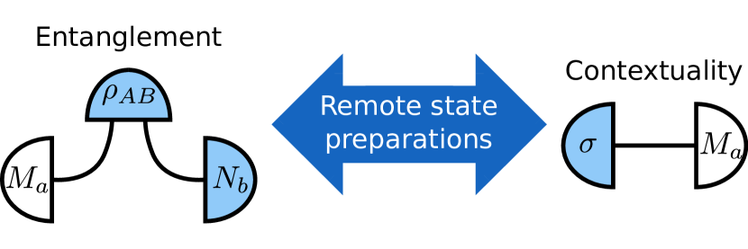
Figure 1: Connections between entanglement in the nonlocal scenario and contextuality in the sequential scenario. In the nonlocal scenario, one considers probability distributions of the type $p(a,b|\rho_{AB})=\operatorname{Tr}[(M_{a}\otimes N_{b})\rho_{AB}]$, where $M_{a}$ and $N_{b}$ describe measurements. In the sequential scenario, Alice prepares a quantum state $\sigma$, transmits it to Bob, leading to the probabilities $p(a|\sigma)=\operatorname{Tr}(\sigma M_{a})$ of his measurements. We show that entanglement in the nonlocal scenario is practically equivalent to noncontextuality in the sequential scenario, if the state $\sigma\sim\operatorname{Tr}_{B}[(\operatorname{\mathds{1}}_{a}\otimes N_{b})\rho_{AB}]$ is prepared remotely by performing a measurement on Bob’s part of the nonlocal scenario.

Are there any connections between quantum resources arising in the nonlocal and the sequential scenario? This is a key question for understanding the quantum advantage in information processing. For quantum key distribution it was already observed some time ago that prepare and measure schemes (like the BB84 protocol) can be mapped to entanglement-based schemes, which allows for a common security analysis of both scenarios based on entanglement theory [3, 16]. More recently, the notion of remote state preparation was used to show that steerability of a quantum state $\rho_{AB}$ corresponds to preparation noncontextuality [17], while steerability of an assemblage corresponds to measurement noncontextuality [18], see also Ref. [12] for a discussion.

In this paper we show that entanglement in the NLS corresponds to P&M contextuality in the SQS. We use the fact that any bipartite quantum state gives rise to some sequential scenario by using a kind of remote state preparation [19, 20]. Then, P&M contextuality in this SQS is precondition of entanglement of the bipartite state. Our results imply that one can map noncontextuality inequalities to entanglement witnesses and that one can use classes of entanglement witnesses to obtain noncontextuality inequalities. Our research was motivated by recent findings on a connection between noncontextuality and the mathematical notion of generalized separability of the identity map [21].

Entanglement and remote preparations

Assume that two remote parties, Alice and Bob, share a bipartite quantum state $\rho_{AB}$. We then say that the bipartite state $\rho_{AB}$ is entangled if it cannot be prepared using local operations and classical communication [22]. This is the same as requiring that the state $\rho_{AB}$ is not separable, i.e., there is no decomposition of the form $\rho_{AB}=\sum_{i}p_{i}\sigma_{i}^{A}\otimes\sigma_{i}^{B}$, where the $p_{i}$ form a probability distribution and $\sigma_{i}^{A}$ and $\sigma_{i}^{B}$ are some states of Alice’s and Bob’s system.

Given a bipartite state $\rho_{AB}$ Bob can apply a measurement to his part of the system and announce the outcome, which results in remotely preparing the state $\operatorname{Tr}_{B}[(\operatorname{\mathds{1}}_{A}\otimes E_{B})\rho_{AB}]$ for Alice. While a single remotely prepared state does not capture the properties of the bipartite state $\rho_{AB}$ shared between Alice and Bob, it is intuitive that the set of all possible remotely preparable states should have some properties based on whether the shared bipartite state $\rho_{AB}$ is entangled or not. In order to investigate this, we denote by $\Lambda_{A}(\rho_{AB})$ the set of all possible states that Bob can remotely prepare for Alice using the shared bipartite state $\rho_{AB}$. Mathematically $\Lambda_{A}(\rho_{AB})$ is defined as

$$\begin{split}\Lambda_{A}(\rho_{AB})=\{&\sigma_{A}\in\operatorname{\mathcal{D}}(\operatorname{\mathcal{H}}_{A}):E_{B}\geq 0\\ &\sigma_{A}=\operatorname{Tr}_{B}[(\operatorname{\mathds{1}}_{A}\otimes E_{B})\rho_{AB}]\},\end{split}$$ (1)

where $\operatorname{\mathcal{H}}_{A}$ is the Hilbert space corresponding to Alice’s system, $\operatorname{\mathcal{D}}(\operatorname{\mathcal{H}}_{A})$ is the set of density matrices on $\operatorname{\mathcal{H}}_{A}$, and $E_{B}\geq 0$ means that $E_{B}$ is a positive semidefinite operator. $\Lambda_{B}(\rho_{AB})$ is defined analogically. Note that these sets of quantum states play a role in recent approaches to tackle the problem of quantum steering [20, 23].

Contextuality

There are several notions of contextuality, here we are interested in so-called preparation & measurement (P&M) noncontextual models in the sense of Spekkens [8, 9]. In this approach one considers a set of preparations and a set of measurements. Two preparations are operationally equivalent if, for all measurements, they give rise to the same probability distribution of outcomes. Analogously, two measurements are operationally equivalent if they result in the same probability distribution for any available state preparation.

In a HV model for this scenario, the assumption of preparation noncontextuality states that two equivalent preparations give rise to the same probability distribution over the HV. Similarly, measurement noncontextuality assumes that equivalent measurements are described by the same response functions. In addition, for a HV model one makes the general assumption of convex linearity. This means that if one chooses randomly one of two preparations, then the resulting probability distribution of the HV is the mixture of the two distributions of the preparations. An analogous assumption is made on random choices of measurements.

In quantum mechanics, state preparations are described by density matrices and measurement probabilities are computed by effects. Thus, a quantum system has a P&M noncontextual HV model if for every density matrix $\rho\in K$ (where $K$ is a convex subset of density matrices that corresponds to the prepareable states) and for every POVM $\operatorname{\mathsf{M}}=\{M_{a}\}$, $0\leq M_{a}\leq\operatorname{\mathds{1}}$, $\sum_{a}M_{a}=\operatorname{\mathds{1}}$, we have

$$\operatorname{Tr}(\rho M_{a})=\sum_{\lambda}p(\lambda|\rho)p(a|\lambda,\operatorname{\mathsf{M}})$$ (2)

where $p(\lambda|\rho)$ is a linear function of $\rho$ and $p(a|\lambda,\operatorname{\mathsf{M}})$ is a linear function of $M_{a}$, see [17] for a detailed explanation.

For our purposes, it is useful to rewrite Eq. (2). Since $p(\lambda|\rho)$ is a linear function of $\rho$ it follows that there are operators $N_{\lambda}$ such that $p(\lambda|\rho)=\operatorname{Tr}(\rho N_{\lambda})$ that satisfy the positivity and normalization conditions:

$$\operatorname{Tr}(\rho N_{\lambda})\geq 0 \sum_{\lambda}\operatorname{Tr}(\rho N_{\lambda})=1,$$ and (3)

for all $\rho\in K$. Note that this does not imply that $N_{\lambda}$ is a POVM. In fact, whenever $K$ is a strict subset of the density matrices, then according to the hyperplane separation theorem [24] there is some $N_{\lambda}$ that satisfies the positivity condition in Eq. (3) that is not a positive semidefinite operator. Analogically, we require that $p(a|\lambda,\operatorname{\mathsf{M}})$ is a linear function of $M_{a}$ so we have $p(a|\lambda,\operatorname{\mathsf{M}})=\operatorname{Tr}(\omega_{\lambda}M_{a})$, where $\omega_{\lambda}\in\operatorname{\mathcal{D}}(\operatorname{\mathcal{H}})$. Putting everything together, we get that there exists preparation & measurement noncontextual HV model for states in $K$ if for every $\rho\in K$ and every POVM $\operatorname{\mathsf{M}}=\{M_{a}\}$ we have

$$\operatorname{Tr}(\rho M_{a})=\sum_{\lambda}\operatorname{Tr}(\rho N_{\lambda})\operatorname{Tr}(\omega_{\lambda}M_{a}).$$ (4)

Main Results

We can directly formulate our first main result:

Theorem 1.

Let $\rho_{AB}$ be a bipartite quantum state and assume that there exists a P&M noncontextual model for the set of states $\Lambda_{A}(\rho_{AB})$ and all possible measurements. Then, $\rho_{AB}$ is separable.

The proof is given in Appendix A. The underlying idea is that in the P&M noncontextual model from Eq. (4) the term $\operatorname{Tr}(\omega_{\lambda}M_{a})$ can be interpreted as measurement on Alice’s side of a separable decomposition $\rho_{AB}=\sum_{\lambda}\omega_{\lambda}\otimes K_{\lambda}$, where Bob’s parts $K_{\lambda}$ in the decomposition are given by $K_{\lambda}=\operatorname{Tr}_{A}[(N_{\lambda}\otimes\operatorname{\mathds{1}}_{B})\rho_{AB}]$.

In the following theorem we will prove that a separable state $\rho_{AB}=\sum_{\lambda}\omega_{\lambda}\otimes K_{\lambda}$ yields remotely preparable set $\Lambda_{A}(\rho_{AB})$ with a preparation & measurement noncontextual model if the operators $K_{\lambda}$ in the separable decomposition can be chosen such that they belong to the linear hull of $\Lambda_{B}(\rho_{AB})$. We will get rid of this condition later by considering robust remote preparations.

Theorem 2.

Let $\rho_{AB}$ be a separable bipartite quantum state with the decomposition $\rho_{AB}=\sum_{\lambda}\omega_{\lambda}\otimes K_{\lambda}$, where $\omega_{\lambda}\geq 0$, $\operatorname{Tr}(\omega_{\lambda})=1$ and $K_{\lambda}\geq 0$. Assume that $K_{\lambda}$ belongs to the linear hull of $\Lambda_{B}(\rho_{AB})$ for all $\lambda$. Then there exists P&M noncontextual model for $\Lambda_{A}(\rho_{AB})$.

The proof can be found in Appendix B. The following example shows that Theorem 2 cannot be directly extended to all states. Consider the separable qubit-ququart state

$$\begin{split}\rho_{AB}&=\frac{1}{4}(|0\rangle\!\langle 0|\otimes|00\rangle\!\langle 00|+|1\rangle\!\langle 1|\otimes|01\rangle\!\langle 01|\\ &+|+\rangle\!\langle+|\otimes|10\rangle\!\langle 10|+|-\rangle\!\langle-|\otimes|11\rangle\!\langle 11|).\end{split}$$ (5)

This does not meet the condition in Theorem 2; at least for the decomposition in Eq. (5) this is obvious: $\Lambda_{B}(\rho_{AB})$ is three-dimensional, while there are four linearly independent $K_{\lambda}$. On the other hand, we have $\Lambda_{A}(\rho_{AB})=\operatorname{conv}(\{|0\rangle\!\langle 0|,|1\rangle\!\langle 1|,|+\rangle\!\langle+|,|-\rangle\!\langle-|\})$, and we will show below that a preparation & measurement noncontextual model for $\Lambda_{A}(\rho_{AB})$ does not exist using violation of the contextuality inequality that we will derive in Proposition 5, see Eq.  (15) below.

Clearly, the linear hull condition in the Theorem 2 is met, if the set $\Lambda_{B}(\rho_{AB})$ spans the entire operator space. Not surprisingly, this is the generic case, and one can get rid of the pathological cases by considering robust remote preparations, i.e., by adding an infinitesimal amount of random separable noise. This idea is summarized in the following theorem, the proof can be found in the Appendix C.

Theorem 3.

Let $\rho_{AB}$ be a separable quantum state. Then for almost all separable quantum states $\tau_{AB}$ there is a $\delta(\tau_{AB})>0$ depending on $\tau_{AB}$, such that for every $\varepsilon\in(0,\delta)$ there exists P&M noncontextual model for $\Lambda_{A}[(1-\varepsilon)\rho_{AB}+\varepsilon\tau_{AB}]$.

Mapping noncontextuality inequalities to entanglement witnesses

Using the results of Theorem 3 one can obtain entanglement witnesses from noncontextuality inequalities. The only caveat is that the noncontextuality inequalities must be formulated in terms of unnormalized states, this is necessary to account for the fact that $\operatorname{Tr}_{B}[(\operatorname{\mathds{1}}_{A}\otimes E_{B})\rho_{AB}]$ is not normalized for $E_{B}\geq 0$. This is because the set of $E_{B}$ such that $\operatorname{Tr}[(\operatorname{\mathds{1}}_{A}\otimes E_{B})\rho_{AB}]=1$ in general depends on $\rho_{AB}$.

We will demonstrate the method using the noncontextuality inequality presented in Ref. [25]. Let $K$ be the set of allowed preparations. By $\operatorname{cone}(K)$ we denote the set of all unnormalized allowed preparations, that is all operators of the form $\mu\tilde{\sigma}$, where $\mu\in\operatorname{\mathbb{R}}$, $\mu\geq 0$ and $\tilde{\sigma}\in K$. Let $\sigma_{t,b}\in\operatorname{cone}(K)$ for $t\in\{1,2,3\}$ and $b\in\{0,1\}$ be such that $\sigma_{*}=\frac{1}{2}(\sigma_{t,0}+\sigma_{t,1})$ is the same for all $t\in\{1,2,3\}$ and let $M_{t,b}$ be positive operators, $M_{t,b}\geq 0$, such that $\frac{1}{3}\sum_{t=1}^{3}M_{t,b}=\frac{\operatorname{\mathds{1}}}{2}$ and $M_{t,0}+M_{t,1}=\operatorname{\mathds{1}}$. In other words, $M_{t,b}$ are three binary POVMs such that their uniform mixture corresponds to the random coin toss. Then the unnormalized version of noncontextuality inequality from Ref. [25] is as follows: If there is a P&M noncontextual model for $K$, then we have

$$\sum_{t=1}^{3}\sum_{b=0}^{1}\operatorname{Tr}(\sigma_{t,b}M_{t,b})\leq 5\operatorname{Tr}(\sigma_{*}).$$ (6)

See Appendix D for the proof of this modified noncontextuality inequality. Using this inequality we obtain the following entanglement witness:

Proposition 4.

Let $\rho_{AB}$ be a separable quantum state. Let $E_{t,b}$ and $M_{t,b}$ be positive operators, $E_{t,b}\geq 0$ and $M_{t,b}\geq 0$, such that $E_{*}=\frac{1}{2}(E_{t,0}+E_{t,1})$, $\frac{1}{3}\sum_{t=1}^{3}M_{t,b}=\frac{\operatorname{\mathds{1}}_{A}}{2}$ and $\operatorname{\mathds{1}}_{A}=M_{t,0}+M_{t,1}$ for all $t\in\{1,2,3\}$ and $b\in\{0,1\}$. Then

$$\sum_{t=1}^{3}\sum_{b=0}^{1}\operatorname{Tr}[(M_{t,b}\otimes E_{t,b})\rho_{AB}]\leq 5\operatorname{Tr}[(\operatorname{\mathds{1}}_{A}\otimes E_{*})\rho_{AB}].$$ (7)

Moreover, there is an entangled state $\rho_{AB}$ that violates Eq. (7) for suitable choice of the operators $E_{t,b}$ and $M_{t,b}$.

The proof follows from Theorem 3, since if $\rho_{AB}$ is separable, then Eq. (7) is satisfied for all $\Lambda_{A}[(1-\varepsilon)\rho_{AB}+\varepsilon\tau_{AB}]$ for all $\varepsilon\in(0,\delta)$. This is then used to construct the corresponding entanglement witness. The full proof can be found in Appendix D.

Being more concrete, one can write down an explicit entanglement witness from observables leading to a violation of the noncontextuality inequality [9]. We consider qubit systems and the Pauli matrices $\sigma_{x},\sigma_{y},\sigma_{z}$. Then we define the effects

$$E_{1,0}=\operatorname{\mathds{1}}+\sigma_{z}, E_{1,1}=\operatorname{\mathds{1}}-\sigma_{z},$$ (8)

$$E_{2,0}=\operatorname{\mathds{1}}+\frac{\sqrt{3}}{2}\sigma_{x}-\frac{1}{2}\sigma_{z}, E_{2,1}=\operatorname{\mathds{1}}-\frac{\sqrt{3}}{2}\sigma_{x}+\frac{1}{2}\sigma_{z},$$ (9)

$$E_{3,0}=\operatorname{\mathds{1}}-\frac{\sqrt{3}}{2}\sigma_{x}-\frac{1}{2}\sigma_{z}, E_{3,1}=\operatorname{\mathds{1}}+\frac{\sqrt{3}}{2}\sigma_{x}+\frac{1}{2}\sigma_{z},$$ (10)

and $M_{t,b}=\frac{1}{2}E_{t,b}$. From this we obtain the entanglement witness $W=2\operatorname{\mathds{1}}_{A}\otimes\operatorname{\mathds{1}}_{B}-\frac{3}{2}(\sigma_{x}\otimes\sigma_{x}+\sigma_{z}\otimes\sigma_{z})$, so for every separable state $\rho_{AB}$ we have

$$\operatorname{Tr}[(\sigma_{x}\otimes\sigma_{x})\rho_{AB}]+\operatorname{Tr}[(\sigma_{z}\otimes\sigma_{z})\rho_{AB}]\leq\frac{4}{3}$$ (11)

which is a weakened version of the well-known witness $\operatorname{Tr}[(\sigma_{x}\otimes\sigma_{x})\rho_{AB}]+\operatorname{Tr}[(\sigma_{z}\otimes\sigma_{z})\rho_{AB}]\leq 1$ [26, 27, 28]; still, the inequality (11) is violated by the maximally entangled state.

Mapping entanglement witnesses to noncontextuality inequalities

This direction is not so straightforward, as we cannot use just a single entanglement witness, but we must map a whole class of entanglement witnesses to get a class of noncontextuality inequalities. We will proceed with an example that showcases this.

We will use a class of entanglement witnesses that comes from the Clauser-Horne-Shimony-Holt (CHSH) inequality [29, 30]. Let $A_{i}$ and $B_{i}$ for $i\in\{1,2\}$ be observables such that $-\operatorname{\mathds{1}}_{A}\leq A_{i}\leq\operatorname{\mathds{1}}_{A}$ and $-\operatorname{\mathds{1}}_{B}\leq B_{i}\leq\operatorname{\mathds{1}}_{B}$ and let $\rho_{AB}$ be a separable state. Then we have $\operatorname{Tr}\{[A_{1}\otimes(B_{1}+B_{2})+A_{2}\otimes(B_{1}-B_{2})]\rho_{AB}\}\leq 2$.

In order to obtain a noncontextuality inequality proceed as follows. Let $B_{i+}$ and $B_{i-}$ be the the positive and negative parts of $B_{i}$, respectively, and denote $\sigma_{i\pm}=\operatorname{Tr}_{B}[(\operatorname{\mathds{1}}_{A}\otimes B_{i\pm})\rho_{AB}]$. Then we have

$$2\geq\operatorname{Tr}\{[A_{1}\otimes(B_{1}+B_{2})+A_{2}\otimes(B_{1}-B_{2})]\rho_{AB}\}=\operatorname{Tr}[(A_{1}+A_{2})(\sigma_{1+}-\sigma_{1-})]+\operatorname{Tr}[(A_{1}-A_{2})(\sigma_{2+}-\sigma_{2-})],$$ (12)

which bears already some formal similarity to the noncontextuality inequality from above. Moreover, we have $B_{i}=B_{i+}-B_{i-}$ and $\left\lvert B_{i}\right\rvert=B_{i+}+B_{i-}$. From $-\operatorname{\mathds{1}}_{B}\leq B_{i}\leq\operatorname{\mathds{1}}_{B}$ it follows that the eigenvalues of $B_{i}$ are from the interval $[-1,1]$ and so we also have $\left\lvert B\right\rvert_{i}\leq\operatorname{\mathds{1}}_{B}$. Let us define $\sigma_{i0}=\operatorname{Tr}_{B}\{[\operatorname{\mathds{1}}_{A}\otimes(\operatorname{\mathds{1}}_{B}-\left\lvert B\right\rvert_{i})]\rho_{AB}\}$ and $\sigma_{*}=\operatorname{Tr}_{B}(\rho_{AB})$. Then we have $\sigma_{1+}+\sigma_{1-}+\sigma_{10}=\sigma_{*}=\sigma_{2+}+\sigma_{2-}+\sigma_{20}$, which is going to play a crucial role in the formulation of the noncontextuality inequality. We obtain:

Proposition 5.

Let $K$ be a set of allowed preparations. Let $\sigma_{*}\in K$ and let $i\in\{1,2\}$, let $\sigma_{i+},\sigma_{i-},\sigma_{i0}\in\operatorname{cone}(K)$ be subnormalized preparations such that

$$\sigma_{1+}+\sigma_{1-}+\sigma_{10}=\sigma_{*}=\sigma_{2+}+\sigma_{2-}+\sigma_{20}.$$ (13)

Let $A_{i}$ be observables such that $-\operatorname{\mathds{1}}\leq A_{i}\leq\operatorname{\mathds{1}}$ for all $i\in\{1,2\}$. If there is a P&M contextual model for $K$, then

$$\operatorname{Tr}[(A_{1}+A_{2})(\sigma_{1+}-\sigma_{1-})]+\operatorname{Tr}[(A_{1}-A_{2})(\sigma_{2+}-\sigma_{2-})]\leq 2.$$ (14)

The proof of Proposition 5 is given in Appendix E. The proof is significantly different from the proof of Proposition 4: There, we showed that Eq. (7) is an entanglement witness as a result of Eq. (6) being noncontextuality inequality. In the proof of Proposition 5 we use Eq. (12) only as an educated guess and we have to prove that Eq. (14) is a noncontextuality inequality by showing that it holds whenever a P&M noncontextual model exists.

In order to construct an explicit violation of the noncontextuality inequality we can consider the equivalent of the standard quantum violation of the CHSH inequality: let $\operatorname{\mathcal{H}}$ be a qubit Hilbert space, $\operatorname{\dim({\mathcal{H}})}=2$, let $\sigma_{x},\sigma_{y},\sigma_{z}$ be the Pauli matrices and let

$$A_{1}=\frac{1}{\sqrt{2}}(\sigma_{x}+\sigma_{z}), A_{2}=\frac{1}{\sqrt{2}}(\sigma_{x}-\sigma_{z}),$$

$$\sigma_{1+}=\frac{1}{2}|+\rangle\!\langle+|, \sigma_{1-}=\frac{1}{2}|-\rangle\!\langle-|,$$ (15)

$$\sigma_{2+}=\frac{1}{2}|0\rangle\!\langle 0|, \sigma_{2-}=\frac{1}{2}|1\rangle\!\langle 1|,$$

where $|+\rangle,|-\rangle$ and $|0\rangle,|1\rangle$ are the eigenbasis of the Pauli operators $\sigma_{x},\sigma_{z}$ respectively. We have $\sigma_{1+}+\sigma_{1-}=\sigma_{2+}+\sigma_{2-}$ and so the constraint (13) is satisfied. We get $\operatorname{Tr}((A_{1}+A_{2})(\sigma_{1+}-\sigma_{1-}))+\operatorname{Tr}((A_{1}-A_{2})(\sigma_{2+}-\sigma_{2-}))=2\sqrt{2}$, hence the inequality (14) is violated.

Let us note that it was shown in Ref. [10] that stabilizer rebit theory, whose state space consists of the convex combinations of the states $|0\rangle\!\langle 0|,|1\rangle\!\langle 1|,|+\rangle\!\langle+|,|-\rangle\!\langle-|$ has a P&M noncontextual model which, at first sight, seems to contradict the presented violation of the noncontextuality inequality (14). There is no contradiction, however, because the observables $A_{1}$ and $A_{2}$ are not included in the stabilizer rebit theory.

Conclusions

Our main results, Theorems 1 and 3, prove that contextuality is a precondition for entanglement and that only entangled states allow for robust remote preparations of contextuality. We have used these results to map noncontextuality inequalities to a class of entanglement witnesses in Proposition 4 and to obtain a class of noncontextuality inequalities from entanglement witnesses in Proposition 5.

Our results provide an insight into why entanglement is a precondition for secure quantum key distribution [3], since if there exists a preparation and measurement noncontextual hidden variable model, then the transmission channel between Alice and Bob can in principle be replaced by a classical channel by the eavesdropper, which makes secure key distribution impossible. As a consequence of our results any experiment which verifies entanglement of a state (e.g., by observing quantum steering or violation of a Bell inequality) immediately verifies P&M contextuality of the induced system. Moreover our results open the path to further transport of results between entanglement and contextuality, it is for example possible to take a contextuality-enabled task and transform it into a remote entanglement-enabled task. Thus our results provide a blueprint for connecting the resource theory of entanglement and contextuality.

Appendix A Appendix A: Proof of Theorem 1

See 1

Proof.

Let $\sigma_{A}\in\Lambda_{A}(\rho_{AB})$ and let $\operatorname{\mathsf{M}}=\{M_{a}\}$ be a POVM on $\operatorname{\mathcal{H}}_{A}$. According to our assumptions there exists P&M noncontextual hidden variable model for $\Lambda_{A}(\rho_{AB})$, thus we have $\operatorname{Tr}(\sigma_{A}M_{a})=\sum_{\lambda}\operatorname{Tr}(\sigma_{A}N_{\lambda})\operatorname{Tr}(\omega_{\lambda}M_{a})$ for some $\omega_{\lambda}\in\operatorname{\mathcal{D}}(\operatorname{\mathcal{H}}_{A})$ and $N_{\lambda}\in\operatorname{\mathcal{B}}(\operatorname{\mathcal{H}}_{A})$ such that $\operatorname{Tr}(\sigma_{A}^{\prime}N_{\lambda})\geq 0$ for all $\sigma_{A}^{\prime}\in\Lambda_{A}(\rho_{AB})$. Since $\sigma_{A}\in\Lambda_{A}(\rho_{AB})$ then there is some $E_{B}\geq 0$ such that $\sigma_{A}=\operatorname{Tr}_{B}[(\operatorname{\mathds{1}}_{A}\otimes E_{B})\rho_{AB}]$ and we have $\operatorname{Tr}(\sigma_{A}M_{a})=\operatorname{Tr}[(M_{a}\otimes E_{B})\rho_{AB}]$ and $\operatorname{Tr}(\sigma_{A}N_{\lambda})=\operatorname{Tr}[(N_{\lambda}\otimes E_{B})\rho_{AB}]$. Moreover we will use that $\operatorname{Tr}[(N_{\lambda}\otimes E_{B})\rho_{AB}]=\operatorname{Tr}\{E_{B}\operatorname{Tr}_{A}[(N_{\lambda}\otimes\operatorname{\mathds{1}}_{B})\rho_{AB}]\}$. Putting everything together we get

$$\begin{split}\operatorname{Tr}[(M_{a}\otimes E_{B})\rho_{AB}]&=\sum_{\lambda}\operatorname{Tr}[(N_{\lambda}\otimes E_{B})\rho_{AB}]\operatorname{Tr}(\omega_{\lambda}M_{a})\\ &=\sum_{\lambda}\operatorname{Tr}[(M_{a}\otimes N_{\lambda}\otimes E_{B})(\omega_{\lambda}\otimes\rho_{AB})]\\ &=\sum_{\lambda}\operatorname{Tr}[(M_{a}\otimes E_{B})(\omega_{\lambda}\otimes\operatorname{Tr}_{A}[(N_{\lambda}\otimes\operatorname{\mathds{1}}_{B})\rho_{AB}])].\end{split}$$ (16)

Since this holds for every $M_{a}$ and $E_{B}$ we must have $\rho_{AB}=\sum_{\lambda}\omega_{\lambda}\otimes\operatorname{Tr}_{A}[(N_{\lambda}\otimes\operatorname{\mathds{1}}_{B})\rho_{AB}]$. In order to prove that $\rho_{AB}$ is separable we only need to prove that $\operatorname{Tr}_{A}[(N_{\lambda}\otimes\operatorname{\mathds{1}}_{B})\rho_{AB}]$ is positive semidefinite for all $\lambda$, but this is straightforward as for any positive semidefinite $F_{B}\in\operatorname{\mathcal{B}}(\operatorname{\mathcal{H}}_{B})$ we have

$$\operatorname{Tr}\{F_{B}\operatorname{Tr}_{A}[(N_{\lambda}\otimes\operatorname{\mathds{1}}_{B})\rho_{AB}]\}=\operatorname{Tr}\{N_{\lambda}\operatorname{Tr}_{B}[(\operatorname{\mathds{1}}_{A}\otimes F_{B})\rho_{AB}]\}=\mu\operatorname{Tr}(N_{\lambda}\sigma_{A}^{\prime})\geq 0$$ (17)

where $\sigma_{A}^{\prime}\in\Lambda_{A}(\rho_{AB})$ and $\mu\geq 0$ are such that $\operatorname{Tr}_{B}[(\operatorname{\mathds{1}}_{A}\otimes F_{B})\rho_{AB}]=\mu\sigma_{A}^{\prime}$. ∎

Appendix B Appendix B: Proof of Theorem 2

Before proceeding to the proof of Theorem 2 we need to introduce two superoperators. Let $\rho_{AB}\in\operatorname{\mathcal{D}}(\operatorname{\mathcal{H}}_{A}\otimes\operatorname{\mathcal{H}}_{B})$ be a bipartite state, then the superoperator $\Psi_{A\to B}^{\rho}:\operatorname{\mathcal{B}}(\operatorname{\mathcal{H}}_{A})\to\operatorname{\mathcal{B}}(\operatorname{\mathcal{H}}_{B})$ is defined as follows: let $X_{A}\in\operatorname{\mathcal{B}}(\operatorname{\mathcal{H}}_{A})$, then

$$\Psi_{A\to B}^{\rho}(X_{A})=\operatorname{Tr}_{A}[(X_{A}\otimes\operatorname{\mathds{1}}_{B})\rho_{AB}].$$ (18)

The superoperator $\Psi_{B\to A}^{\rho}:\operatorname{\mathcal{B}}(\operatorname{\mathcal{H}}_{B})\to\operatorname{\mathcal{B}}(\operatorname{\mathcal{H}}_{A})$ is defined analogically. Moreover we can express the remotely preparable sets using the superoperator $\Psi_{B\to A}^{\rho}$ as $\Lambda_{A}(\rho_{AB})=\{\sigma_{A}\in\operatorname{\mathcal{D}}(\operatorname{\mathcal{H}}_{A}):\>\sigma_{A}=\Psi_{B\to A}^{\rho}(E_{B}),E_{B}\geq 0\}$.

Let $\{X_{i}^{A}\}_{i=1}^{\dim(\operatorname{\mathcal{H}}_{A})^{2}}$ and $\{Y_{j}^{B}\}_{j=1}^{\dim(\operatorname{\mathcal{H}}_{B})^{2}}$ be an orthonormal operator basis of $B(\operatorname{\mathcal{H}}_{A})$ and $B(\operatorname{\mathcal{H}}_{B})$ respectively, i.e., $\operatorname{Tr}(X_{i}^{A}X_{j}^{A})=\operatorname{Tr}(Y_{i}^{B}Y_{j}^{B})=\delta_{ij}$, then the basis can be chosen such that $\rho_{AB}=\sum_{i=1}^{N}p_{i}X_{i}^{A}\otimes Y_{i}^{B}$, where $N=\max[\dim(\operatorname{\mathcal{H}}_{A})^{2},\dim(\operatorname{\mathcal{H}}_{B})^{2}]$ and $p_{i}\geq 0$, this is essentially Schmidt decomposition applied to $\rho_{AB}$ as a vector in $\operatorname{\mathcal{B}}(\operatorname{\mathcal{H}}_{A})\otimes\operatorname{\mathcal{B}}(\operatorname{\mathcal{H}}_{B})$. Let $I_{+}$ be the index set defined as $I_{+}=\{i:p_{i}>0\}$. We then define the superoperator $\Pi_{A}^{\rho}:\operatorname{\mathcal{B}}(\operatorname{\mathcal{H}}_{A})\to\operatorname{\mathcal{B}}(\operatorname{\mathcal{H}}_{A})$ as follows:

$$\Pi_{A}^{\rho}(\sum_{i=1}^{\dim(\operatorname{\mathcal{H}}_{A})^{2}}\alpha_{i}X_{i}^{A})=\sum_{i\in I_{+}}\alpha_{i}X_{i}^{A}.$$ (19)

$\Pi_{B}^{\rho}:\operatorname{\mathcal{B}}(\operatorname{\mathcal{H}}_{B})\to\operatorname{\mathcal{B}}(\operatorname{\mathcal{H}}_{B})$ is defined analogically.

The superoperators $\Pi_{A}^{\rho}$ and $\Pi_{B}^{\rho}$ will appear in our calculations for the following reason: the superoperator $\Psi_{B\to A}^{\rho}$ is not necessarily invertible, but we can invert it on its support. $\Pi_{A}^{\rho}$ and $\Pi_{B}^{\rho}$ are projections on the support of $\Psi_{B\to A}^{\rho}$ and so they will appear because we will use the pseudo-inverse of $\Psi_{B\to A}^{\rho}$.

Lemma.

Let $\rho_{AB}$ be a separable bipartite quantum state with the decomposition $\rho_{AB}=\sum_{\lambda}\omega_{\lambda}\otimes K_{\lambda}$, where $\omega_{\lambda}\geq 0$, $\operatorname{Tr}(\omega_{\lambda})=1$ and $K_{\lambda}\geq 0$. Assume that we have $\Pi_{B}^{\rho}(K_{\lambda})\geq 0$ for all $\lambda$. Then there exists P&M noncontextual model for $\Lambda_{A}(\rho_{AB})$.

Proof.

Let $\{X_{i}^{A}\}_{i=1}^{\dim(\operatorname{\mathcal{H}}_{A})^{2}}$ and $\{Y_{j}^{B}\}_{j=1}^{\dim(\operatorname{\mathcal{H}}_{B})^{2}}$ be orthonormal operator basis of $B(\operatorname{\mathcal{H}}_{A})$ and $B(\operatorname{\mathcal{H}}_{B})$ respectively such that $\rho_{AB}=\sum_{i=1}^{N}p_{i}X_{i}^{A}\otimes Y_{i}^{B}$, where $N=\max[\dim(\operatorname{\mathcal{H}}_{A})^{2},\dim(\operatorname{\mathcal{H}}_{B})^{2}]$ and $p_{i}\geq 0$. Let $\sigma_{A}\in\Lambda_{A}(\rho_{AB})$ and let $E_{B}\in\operatorname{\mathcal{B}}(\operatorname{\mathcal{H}}_{B})$, $E_{B}\geq 0$, be the corresponding operator such that $\sigma_{A}=\operatorname{Tr}_{B}[(\operatorname{\mathds{1}}_{A}\otimes E_{B})\rho_{AB}]$. Then $E_{B}=\sum_{i=1}^{\dim(\operatorname{\mathcal{H}}_{B})^{2}}\beta_{i}Y_{i}^{B}$ and we have

$$\sigma_{A}=\operatorname{Tr}_{B}[(\operatorname{\mathds{1}}_{A}\otimes E_{B})\rho_{AB}]=\Psi_{B\to A}^{\rho}(E_{B})=\sum_{i\in I_{+}}\beta_{i}p_{i}X_{i}^{A}.$$ (20)

We will now define a superoperator $\Phi:\operatorname{\mathcal{B}}(\operatorname{\mathcal{H}}_{A})\to\operatorname{\mathcal{B}}(\operatorname{\mathcal{H}}_{B})$ that will act as the pseudo-inverse to the superoperator $\Psi_{B\to A}^{\rho}$ as follows: let $F_{A}\in\operatorname{\mathcal{B}}(\operatorname{\mathcal{H}}_{A})$, then $F_{A}=\sum_{i=1}^{\dim(\operatorname{\mathcal{H}}_{A})^{2}}\alpha_{i}X_{i}^{A}$ and we define $\Phi(F_{A})=\sum_{i\in I_{+}}\frac{\alpha_{i}}{p_{i}}Y_{i}^{B}$. We clearly have

$$(\Phi\circ\Psi_{B\to A}^{\rho})(E_{B})=\Pi_{B}^{\rho}(E_{B}),$$ (21)

where $\circ$ denotes the concatenation of superoperators. Moreover it follows that $\Psi_{B\to A}^{\rho}(E_{B})=(\Psi_{B\to A}^{\rho}\circ\Pi_{B}^{\rho})(E_{B})$. Let $\operatorname{\mathsf{M}}=\{M_{a}\}$ be a POVM, then we have

$$\operatorname{Tr}(\sigma_{A}M_{a})=\operatorname{Tr}[(M_{a}\otimes E_{B})\rho_{AB}]=\operatorname{Tr}\{[M_{a}\otimes\Pi_{B}^{\rho}(E_{B})]\rho_{AB}\}=\sum_{\lambda}\operatorname{Tr}(\omega_{\lambda}M_{a})\operatorname{Tr}[\Pi_{B}^{\rho}(E_{B})K_{\lambda}].$$ (22)

Using Eq. (21) we get

$$\operatorname{Tr}(\sigma_{A}M_{a})=\sum_{\lambda}\operatorname{Tr}[\Psi_{B\to A}^{\rho}(E_{B})\Phi^{*}(K_{\lambda})]\operatorname{Tr}(\omega_{\lambda}M_{a})=\sum_{\lambda}\operatorname{Tr}[\sigma_{A}\Phi^{*}(K_{\lambda})]\operatorname{Tr}(\omega_{\lambda}M_{a})$$ (23)

where $\Phi^{*}$ is the adjoint superoperator to $\Phi$. Denoting $\Phi^{*}(K_{\lambda})=N_{\lambda}$ we get

$$\operatorname{Tr}(\sigma_{A}M_{a})=\sum_{\lambda}\operatorname{Tr}(\sigma_{A}N_{\lambda})\operatorname{Tr}(\omega_{\lambda}M_{a})$$ (24)

which is the desired result, we only need to check that $N_{\lambda}$ satisfies the positivity and normalization conditions (3).

Let $\sigma_{A}\in\Lambda_{A}(\rho_{AB})$ be given as $\sigma_{A}=\Psi_{B\to A}^{\rho}(E_{B})$ for some $E_{B}\in\operatorname{\mathcal{B}}(\operatorname{\mathcal{H}}_{B})$, $E_{B}\geq 0$, then we have

$$\operatorname{Tr}(\sigma_{A}N_{\lambda})=\operatorname{Tr}[\Phi(\sigma_{A})K_{\lambda}]=\operatorname{Tr}[\Pi_{B}^{\rho}(E_{B})K_{\lambda}]=\operatorname{Tr}[E_{B}\Pi_{B}^{\rho}(K_{\lambda})]\geq 0$$ (25)

since $\Pi_{B}^{\rho}(K_{\lambda})\geq 0$ according to the assumptions of the theorem. To check normalization note that due to the adjoint version of Eq. (21) we have that $\Phi^{*}$ is the pseudo-inverse of the superoperator $\Psi_{A\to B}^{\rho}$. Using $\sum_{\lambda}K_{\lambda}=\operatorname{Tr}_{A}(\rho_{AB})=\operatorname{Tr}_{A}[(\operatorname{\mathds{1}}_{A}\otimes\operatorname{\mathds{1}}_{B})\rho_{AB}]$ we get that $\Phi^{*}(\sum_{\lambda}K_{\lambda})=\Pi_{A}^{\rho}(\operatorname{\mathds{1}}_{A})$ and so we have $\sum_{\lambda}N_{\lambda}=\Phi^{*}(\sum_{\lambda}K_{\lambda})=\Pi_{A}^{\rho}(\operatorname{\mathds{1}}_{A})$. It follows that $\sum_{\lambda}\operatorname{Tr}(\sigma_{A}N_{\lambda})=\operatorname{Tr}[\sigma_{A}\Pi_{A}^{\rho}(\operatorname{\mathds{1}})]=\operatorname{Tr}(\sigma_{A})=1$ because $\Pi_{A}^{\rho}(\sigma_{A})=\sigma_{A}$. ∎

See 2

Proof.

The result follows from the previous lemma. Since for every $\sigma\in\Lambda_{B}(\rho_{AB})$ we have $\Pi^{\rho}_{B}(\sigma)=\sigma$, it follows that if $K_{\lambda}$ belongs to the linear hull of of $\Lambda_{B}(\rho_{AB})$ then we have $\Pi^{\rho}_{B}(K_{\lambda})=K_{\lambda}\geq 0$. ∎

Appendix C Appendix C: Proof of Theorem 3

See 3

Proof.

We will assume that $n=\dim(\operatorname{\mathcal{H}}_{A})=\dim(\operatorname{\mathcal{H}}_{B})$ as we can always embed smaller Hilbert spaces into larger ones. And let $\tau_{AB}\in\operatorname{\mathcal{D}}(\operatorname{\mathcal{H}}_{A}\otimes\operatorname{\mathcal{H}}_{B})$ be a randomly selected separable state. Since $\dim(\operatorname{\mathcal{H}}_{A})=\dim(\operatorname{\mathcal{H}}_{B})=n$, we can represent the superoperators $\Psi_{B\to A}^{\rho}$ and $\Psi_{B\to A}^{\tau}$ by $n^{2}\times n^{2}$ matrices $M(\Psi_{B\to A}^{\rho})$ and $M(\Psi_{B\to A}^{\tau})$. Moreover since $\tau_{AB}$ is randomly selected, we have $\det[M(\Psi_{B\to A}^{\tau})]\neq 0$, since almost all matrices have non-zero determinants.

It follows that the matrix corresponding to the superoperator $\Psi_{B\to A}^{(1-\varepsilon)\rho+\varepsilon\tau}$ is $(1-\varepsilon)M(\Psi_{B\to A}^{\rho})+\varepsilon M(\Psi_{B\to A}^{\tau})$. In order to finish the proof we want to show that there is some $\delta\in(0,1)$ such that for all $\varepsilon\in(0,\delta)$ we have $\det[(1-\varepsilon)M(\Psi_{B\to A}^{\rho})+\varepsilon M(\Psi_{B\to A}^{\tau})]\neq 0$, then it follows that the superoperator $\Psi_{B\to A}^{(1-\varepsilon)\rho_{AB}+\varepsilon\tau_{AB}}$ is invertible.

We have that $\det[(1-\varepsilon)M(\Psi_{B\to A}^{\rho})+\varepsilon M(\Psi_{B\to A}^{\tau})]$ is either constant in $\varepsilon$ or a polynomial of finite order. Since the superoperator $\Psi_{B\to A}^{\tau}$ is invertible we must have $\det[M(\Psi_{B\to A}^{\tau})]\neq 0$. Therefore if $\det[(1-\varepsilon)M(\Psi_{B\to A}^{\rho})+\varepsilon M(\Psi_{B\to A}^{\tau})]$ is constant, then $\det[(1-\varepsilon)M(\Psi_{B\to A}^{\rho})+\varepsilon M(\Psi_{B\to A}^{\tau})]\neq 0$ for all $\varepsilon\in[0,1]$ and the result follows. If $\det[(1-\varepsilon)M(\Psi_{B\to A}^{\rho})+\varepsilon M(\Psi_{B\to A}^{\tau})]$ is not constant, then let $\delta$ be the smallest root of $\det[(1-\varepsilon)M(\Psi_{B\to A}^{\rho})+\varepsilon M(\Psi_{B\to A}^{\tau})]$ from the interval $(0,1)$. It follows that for all $\varepsilon\in(0,\delta)$ we have $\det[(1-\varepsilon)M(\Psi_{B\to A}^{\rho})+\varepsilon M(\Psi_{B\to A}^{\tau})]\neq 0$ and thus the corresponding map is invertible. ∎

One can construct suitable $\tau_{AB}$ explicitly as follows: Let $\frac{\operatorname{\mathds{1}}_{A}}{\sqrt{n}},\tilde{X}_{i}^{A}\in\operatorname{\mathcal{B}}(\operatorname{\mathcal{H}}_{A})$ and $\frac{\operatorname{\mathds{1}}_{B}}{\sqrt{n}},\tilde{Y}_{i}^{B}\in\operatorname{\mathcal{B}}(\operatorname{\mathcal{H}}_{B})$ be orthonormal basis, i.e., $\operatorname{Tr}(\tilde{X}_{i}^{A})=\operatorname{Tr}(\tilde{Y}_{i}^{B})=0$ and $\operatorname{Tr}(\tilde{X}_{i}^{A}\tilde{X}_{j}^{A})=\operatorname{Tr}(\tilde{Y}_{i}^{A}\tilde{Y}_{j}^{B})=\delta_{ij}$. Note that these are different basis than the Schmidt basis used in previous constructions. We then define $\tau_{AB}\in\operatorname{\mathcal{B}}(\operatorname{\mathcal{H}}_{A}\otimes\operatorname{\mathcal{H}}_{B})$ as $\tau_{AB}=\frac{\operatorname{\mathds{1}}_{A}\otimes\operatorname{\mathds{1}}_{B}}{n}+\mu\sum_{i}\tilde{X}_{i}^{A}\otimes\tilde{Y}_{i}^{B}$, where $\mu>0$. It follows that we can always choose $\mu$ so small that $\tau_{AB}\geq 0$, moreover such that $\tau_{AB}$ is a separable state. Let $E_{B}\in\operatorname{\mathcal{B}}(\operatorname{\mathcal{H}}_{B})$, then $E_{B}=\beta_{1}\frac{\operatorname{\mathds{1}}_{B}}{\sqrt{n}}+\sum_{i}\beta_{i}\tilde{Y}_{i}^{B}$ and we have $\operatorname{Tr}_{B}((\operatorname{\mathds{1}}_{A}\otimes E_{B})\tau_{AB})=\beta_{1}\frac{\operatorname{\mathds{1}}_{A}}{\sqrt{n}}+\mu\sum_{i}\beta_{i}\tilde{X}_{i}^{B}$, from which it follows that the superoperator $\Psi_{B\to A}^{\tau}$ is invertible. It then follows that $\Psi_{B\to A}^{(1-\varepsilon)\rho+\varepsilon\tau}$ is also invertible for $\varepsilon\in(0,\delta)$ for suitable choice of $\delta$.

Appendix D Appendix D: Proof of Proposition 4

The following result is a restatement of a known noncontextuality inequality [25], our only modification is that we allow for unnormalized states.

Proposition.

Let $K\subset\operatorname{\mathcal{D}}(\operatorname{\mathcal{H}})$ be the set of allowed preparations and let $\operatorname{cone}(K)$ denote the set of all unnormalized allowed preparations, that is all operators of the form $\mu\tilde{\sigma}$, where $\mu\in\operatorname{\mathbb{R}}$, $\mu\geq 0$ and $\tilde{\sigma}\in K$. Let $\sigma_{t,b}\in\operatorname{cone}(K)$ for $t\in\{1,2,3\}$ and $b\in\{0,1\}$ be such that $\sigma_{*}=\frac{1}{2}(\sigma_{t,0}+\sigma_{t,1})=\frac{1}{2}(\sigma_{t^{\prime},0}+\sigma_{t^{\prime},1})$ for all $t,t^{\prime}\in\{1,2,3\}$ and let $M_{t,b}\in\operatorname{\mathcal{B}}(\operatorname{\mathcal{H}})$ be positive operators, $M_{t,b}\geq 0$, such that $\frac{1}{3}\sum_{t=1}^{3}M_{t,b}=\frac{\operatorname{\mathds{1}}}{2}$ and $M_{t,0}+M_{t,1}=\operatorname{\mathds{1}}$ for all $t$. If there is preparation and measurement noncontextual hidden variable model for $K$, then we have

$$\sum_{t=1}^{3}\sum_{b=0}^{1}\operatorname{Tr}(\sigma_{t,b}M_{t,b})\leq 5\operatorname{Tr}(\sigma_{*}).$$ (26)

Proof.

Using Eq. (4) we get

$$\begin{split}\sum_{t=1}^{3}\sum_{b=0}^{1}\operatorname{Tr}(\sigma_{t,b}M_{t,b})&=\sum_{t=1}^{3}\sum_{b=0}^{1}\sum_{\lambda}\operatorname{Tr}(\sigma_{t,b}N_{\lambda})\operatorname{Tr}(\omega_{\lambda}M_{t,b})\leq\sum_{t=1}^{3}\sum_{\lambda}\max_{b}[\operatorname{Tr}(\omega_{\lambda}M_{t,b})]\sum_{b=0}^{1}\operatorname{Tr}(\sigma_{t,b}N_{\lambda})\\ &=2\sum_{t=1}^{3}\sum_{\lambda}\max_{b}[\operatorname{Tr}(\omega_{\lambda}M_{t,b})]\operatorname{Tr}(\sigma_{*}N_{\lambda})\leq 6\max_{\lambda}\{\frac{1}{3}\sum_{t=1}^{3}\max_{b}[\operatorname{Tr}(\omega_{\lambda}M_{t,b})]\}\sum_{\lambda}\operatorname{Tr}(\sigma_{*}N_{\lambda})\\ &\leq 5\operatorname{Tr}(\sigma_{*}),\end{split}$$ (27)

where we have used that $\frac{1}{3}\sum_{t=1}^{3}\max_{b}[\operatorname{Tr}(\omega_{\lambda}M_{t,b})]\leq\frac{5}{6}$, which is a standard step in proving the origin noncontextuality inequality, see [25, 9]. To see that $\sum_{\lambda}\operatorname{Tr}(\sigma_{*}N_{\lambda})=\operatorname{Tr}(\sigma_{*})$ simply note that $\sigma_{*}\in\operatorname{cone}(K)$ and so $\sigma_{*}=\operatorname{Tr}(\sigma_{*})\tilde{\sigma}_{*}$ where $\tilde{\sigma}_{*}\in K$. Then $\sum_{\lambda}\operatorname{Tr}(\sigma_{*}N_{\lambda})=\operatorname{Tr}(\sigma_{*})\sum_{\lambda}\operatorname{Tr}(\tilde{\sigma}_{*}N_{\lambda})=\operatorname{Tr}(\sigma_{*})$ as a result of the normalization of $N_{\lambda}$. ∎

See 4

Proof.

The proof is straightforward: assume that $\rho_{AB}$ is separable and let $\tau_{AB}$ be a separable state such that there exists preparation and measurement noncontextual hidden variable model for $\Lambda_{A}((1-\varepsilon)\rho_{AB}+\varepsilon\tau_{AB})$ for all $\varepsilon\in(0,\delta)$ for suitable $\delta\in(0,1)$. Denote $\sigma_{t,b,\varepsilon}=\operatorname{Tr}_{B}((\operatorname{\mathds{1}}_{A}\otimes E_{t,b})((1-\varepsilon)\rho_{AB}+\varepsilon\tau_{AB}))$ and $\sigma_{*,\varepsilon}=\operatorname{Tr}_{B}((\operatorname{\mathds{1}}_{A}\otimes E_{*})((1-\varepsilon)\rho_{AB}+\varepsilon\tau_{AB}))$, then Eq. (6) becomes $\sum_{t=1}^{3}\sum_{b=0}^{1}\operatorname{Tr}(\sigma_{t,b,\varepsilon}M_{t,b})\leq 5\operatorname{Tr}(\sigma_{*,\varepsilon})$. We thus get

$$\sum_{t=1}^{3}\sum_{b=0}^{1}\operatorname{Tr}\{[E_{t,b}\otimes M_{t,b}][(1-\varepsilon)\rho_{AB}+\varepsilon\tau_{AB}]\}\leq 5\operatorname{Tr}\{[E_{*}\otimes\operatorname{\mathds{1}}_{B}][(1-\varepsilon)\rho_{AB}+\varepsilon\tau_{AB}]\}$$ (28)

for all $\varepsilon\in(0,\delta)$. Taking the limit $\varepsilon\to 0^{+}$ yields Eq. (7).

To show that there is an entangled state that violates Eq. (7) simply assume that $\sigma_{t,b}$ and $M_{t,b}$ are states and POVMs that violate Eq. (7), it is known that such states and POVMs exist [25, 9]. Let $|\phi^{+}\rangle=\frac{1}{\sqrt{\dim(\operatorname{\mathcal{H}})}}\sum_{i=1}^{\dim(\operatorname{\mathcal{H}})}|ii\rangle$ be the maximally entangled state and take $\rho_{AB}=|\phi^{+}\rangle\!\langle\phi^{+}|$. Take $E_{t,b}=\dim(\operatorname{\mathcal{H}})\sigma_{t,b}^{\intercal}$, where $A^{\intercal}$ is the transposition of $A$ with respect to the basis $|i\rangle$. Then we have $\operatorname{Tr}_{B}[(\operatorname{\mathds{1}}_{A}\otimes E_{t,b})\rho_{AB}]=\sigma_{t,b}$ and so Eq. (7) must be violated because the corresponding noncontextuality inequality is violated. ∎

Appendix E Appendix E: Proof of Proposition 5

See 5

Proof.

In order to shorten the notation let us denote

$$\Xi(A,\sigma)=\operatorname{Tr}[(A_{1}+A_{2})(\sigma_{1+}-\sigma_{1-})]+\operatorname{Tr}[(A_{1}-A_{2})(\sigma_{2+}-\sigma_{2-})].$$ (29)

The proof is straightforward: assume that there is preparation and measurement noncontextual hidden variable model for $K\subset\operatorname{\mathcal{D}}(\operatorname{\mathcal{H}})$. Then due to the linearity of Eq. (4) we have $\operatorname{Tr}(\sigma_{i\pm}A_{j})=\sum_{\lambda}\operatorname{Tr}(\sigma_{i\pm}N_{\lambda})\operatorname{Tr}(\omega_{\lambda}A_{j})$ for all $i,j\in\{1,2\}$, this follows for example from $A_{i}=2M_{i}-\operatorname{\mathds{1}}$ where $0\leq M_{i}\leq\operatorname{\mathds{1}}$ is an appropriate operator. We thus get

$$\begin{split}\Xi(A,\sigma)&=\sum_{\lambda}\operatorname{Tr}[N_{\lambda}(\sigma_{1+}-\sigma_{1-})]\operatorname{Tr}[(A_{1}+A_{2})\omega_{\lambda}]+\sum_{\lambda}\operatorname{Tr}[N_{\lambda}(\sigma_{2+}-\sigma_{2-})]\operatorname{Tr}[(A_{1}-A_{2})\omega_{\lambda}]\\ &=\sum_{\lambda}\operatorname{Tr}[N_{\lambda}(\sigma_{1+}-\sigma_{1-}+\sigma_{2+}-\sigma_{2-})]\operatorname{Tr}(A_{1}\omega_{\lambda})+\sum_{\lambda}\operatorname{Tr}[N_{\lambda}(\sigma_{1+}-\sigma_{1-}-\sigma_{2+}+\sigma_{2-})]\operatorname{Tr}(A_{2}\omega_{\lambda})\\ &\leq\sum_{\lambda}\left\lvert\operatorname{Tr}[N_{\lambda}(\sigma_{1+}-\sigma_{1-}+\sigma_{2+}-\sigma_{2-})]\right\rvert+\sum_{\lambda}\left\lvert\operatorname{Tr}[N_{\lambda}(\sigma_{1+}-\sigma_{1-}-\sigma_{2+}+\sigma_{2-})]\right\rvert,\end{split}$$ (30)

where we have used that $\operatorname{Tr}(A_{i}\omega_{\lambda})\in[-1,1]$ for all $i\in\{1,2\}$ and all $\lambda$. Let us fix $\lambda$ and let us inspect the term $\left\lvert\operatorname{Tr}[N_{\lambda}(\sigma_{1+}-\sigma_{1-}+\sigma_{2+}-\sigma_{2-})]\right\rvert+\left\lvert\operatorname{Tr}[N_{\lambda}(\sigma_{1+}-\sigma_{1-}-\sigma_{2+}+\sigma_{2-})]\right\rvert=\xi_{\lambda}$. There are four options on how the signs can be assigned: if $\operatorname{Tr}[N_{\lambda}(\sigma_{1+}-\sigma_{1-}+\sigma_{2+}-\sigma_{2-})]\geq 0$ and $\operatorname{Tr}[N_{\lambda}(\sigma_{1+}-\sigma_{1-}-\sigma_{2+}+\sigma_{2-})]\geq 0$ we get

$$\xi_{\lambda}=\operatorname{Tr}[N_{\lambda}(\sigma_{1+}-\sigma_{1-}+\sigma_{2+}-\sigma_{2-})]+\operatorname{Tr}[N_{\lambda}(\sigma_{1+}-\sigma_{1-}-\sigma_{2+}+\sigma_{2-})]=2\operatorname{Tr}[N_{\lambda}(\sigma_{1+}-\sigma_{1-})]\leq 2\operatorname{Tr}(N_{\lambda}\sigma_{*}),$$ (31)

where the last inequality follows from Eq. (13) and from the positivity condition in Eq. (3). If $\operatorname{Tr}[N_{\lambda}(\sigma_{1+}-\sigma_{1-}+\sigma_{2+}-\sigma_{2-})]\geq 0$ and $\operatorname{Tr}[N_{\lambda}(\sigma_{1+}-\sigma_{1-}-\sigma_{2+}+\sigma_{2-})]<0$ we get

$$\xi_{\lambda}=\operatorname{Tr}[N_{\lambda}(\sigma_{1+}-\sigma_{1-}+\sigma_{2+}-\sigma_{2-})]-\operatorname{Tr}[N_{\lambda}(\sigma_{1+}-\sigma_{1-}-\sigma_{2+}+\sigma_{2-})]=2\operatorname{Tr}[N_{\lambda}(\sigma_{2+}-\sigma_{2-})]\leq 2\operatorname{Tr}(N_{\lambda}\sigma_{*}),$$ (32)

if $\operatorname{Tr}[N_{\lambda}(\sigma_{1+}-\sigma_{1-}+\sigma_{2+}-\sigma_{2-})]<0$ and $\operatorname{Tr}[N_{\lambda}(\sigma_{1+}-\sigma_{1-}-\sigma_{2+}+\sigma_{2-})]\geq 0$ we get

$$\xi_{\lambda}=-\operatorname{Tr}[N_{\lambda}(\sigma_{1+}-\sigma_{1-}+\sigma_{2+}-\sigma_{2-})]+\operatorname{Tr}[N_{\lambda}(\sigma_{1+}-\sigma_{1-}-\sigma_{2+}+\sigma_{2-})]=2\operatorname{Tr}[N_{\lambda}(\sigma_{2-}-\sigma_{2+})]\leq 2\operatorname{Tr}(N_{\lambda}\sigma_{*}),$$ (33)

if $\operatorname{Tr}[N_{\lambda}(\sigma_{1+}-\sigma_{1-}+\sigma_{2+}-\sigma_{2-})]<0$ and $\operatorname{Tr}[N_{\lambda}(\sigma_{1+}-\sigma_{1-}-\sigma_{2+}+\sigma_{2-})]<0$ we get

$$\xi_{\lambda}=-\operatorname{Tr}[N_{\lambda}(\sigma_{1+}-\sigma_{1-}+\sigma_{2+}-\sigma_{2-})]-\operatorname{Tr}[N_{\lambda}(\sigma_{1+}-\sigma_{1-}-\sigma_{2+}+\sigma_{2-})]=2\operatorname{Tr}[N_{\lambda}(\sigma_{1-}-\sigma_{1+})]\leq 2\operatorname{Tr}(N_{\lambda}\sigma_{*}).$$ (34)

We thus have $\Xi(A,\sigma)\leq 2\sum_{\lambda}\operatorname{Tr}(N_{\lambda}\sigma_{*})=2$ where we have used that $\sigma_{*}\in K$ and the normalization condition in Eq. (3). ∎