BASS XXXIII: Swift-BAT blazars and their jets through cosmic time

Abstract

We derive the most up-to-date Swift-Burst Alert Telescope (BAT) blazar luminosity function in the $14-195\,\rm keV$ range, making use of a clean sample of 118 blazars detected in the BAT 105-month survey catalog, with newly obtained redshifts from the BAT AGN Spectroscopic Survey (BASS). We determine the best-fit X-ray luminosity function for the whole blazar population, as well as for Flat Spectrum Radio Quasars (FSRQs) alone. The main results are: (1) at any redshift, BAT detects the most luminous blazars, above any possible break in their luminosity distribution, which means we cannot differentiate between density and luminosity evolution; (2) the whole blazar population, dominated by FSRQs, evolves positively up to redshift $z\sim 4.3$, confirming earlier results and implying lower number densities of blazars at higher redshifts than previously estimated. The contribution of this source class to the Cosmic X-ray Background at $14-195\,\rm keV$ can range from 5-18%, while possibly accounting for 100% of the MeV background. We also derived the average $14\,\rm keV-10\,\rm GeV$ SED for BAT blazars, which allows us to predict the number counts of sources in the MeV range, as well as the expected number of high-energy ($>$100 TeV) neutrinos. A mission like COSI, will detect 40 MeV blazars and 2 coincident neutrinos. Finally, taking into account beaming selection effects, the distribution and properties of the parent population of these extragalactic jets are derived. We find that the distribution of viewing angles is quite narrow, with most sources aligned within $<5\degree$ of the line of sight. Moreover, the average Lorentz factor, $<\Gamma>=8-12$, is lower than previously suggested for these powerful sources.

1 Introduction

The extragalactic universe is permeated at every observable wavelength by a rather uniform glow (e.g., Hauser & Dwek, 2001; Dwek & Krennrich, 2013; Gilli, 2013; Ackermann et al., 2015; Mozdzen et al., 2017; Fermi-LAT Collaboration et al., 2018a; Desai et al., 2019; Planck Collaboration et al., 2019). Referred to as “backgrounds”, in some cases they are attributed to the integrated emission of many unresolved sources. In others they can carry the imprint of truly diffuse emission processes, as well as signatures of the cosmic web structure (e.g., He et al., 2018). At the highest energies, the so-called extragalactic cosmic X- (CXB, $F_{\rm CXB}\sim 10^{-7}\,\rm erg~{}cm^{-2}~{}s^{-1}~{}sr^{-1}$, Ajello et al., 2008; Gilli, 2013) and $\gamma$-ray background (EGB, $F_{\rm EGB}\sim 10^{-9}\,\rm erg~{}cm^{-2}~{}s^{-1}~{}sr^{-1}$, Ackermann et al., 2015) can be accounted for in terms of unresolved sources (e.g., Churazov et al., 2007; Ajello et al., 2009; Ueda et al., 2014; Aird et al., 2015; Ajello et al., 2015; Cappelluti et al., 2017; Ananna et al., 2020; Marcotulli et al., 2020a).

In particular, in the hard X-ray regime ($\rm E>10\,\rm keV$) the CXB is dominated by supermassive black holes accreting gas at the centers of galaxies. A fraction ($\sim 10\%$) of these active galactic nuclei (AGNs) powers relativistic jets which, when pointing close to our line of sight, are called blazars. Canonically, blazars are differentiated into two major sub-classes, the Flat-Spectrum Radio Quasars (FSRQs) and BL Lacertae objects (BL Lacs), distinguished by the presence or weakness/absence of optical emission lines stronger than $5$Å in equivalent width (e.g., Schmitt, 1968; Stein et al., 1976). Fueled by the most massive black holes ($M_{\rm BH}>10^{8}M_{\odot}$), the jets’ peculiar orientation enhances their emission and renders them visible up to very high-redshifts ($z>4$, see e.g., Romani, 2006; Sbarrato et al., 2015; An & Romani, 2018; Marcotulli et al., 2020b; An & Romani, 2020). If we could understand how the blazar population evolved through cosmic time, this would enable us to trace both the jets (e.g., Ajello et al., 2012b) and supermassive black holes (e.g., Sbarrato et al., 2015) formation and evolution into the early universe (e.g., Berti & Volonteri, 2008; Volonteri, 2010). Indeed, what triggers and powers jet activity, and what is its relation to supermassive black hole accretion are still open questions in astrophysics. The fact that these blazars usually reside in old, already evolved, massive elliptical galaxies (e.g., Urry et al., 1999; Falomo et al., 2000; Scarpa et al., 2000; Chiaberge & Marconi, 2011; Olguín-Iglesias et al., 2016) has provided some evidence possibly linking major merger events (more frequent in the high-redshift universe) as triggers for jet activity, as well as being a preferred channel for rapid supermassive black hole accretion (see Mayer et al., 2010; Chiaberge et al., 2015; Paliya et al., 2020b). Moreover, it has been proposed that these jets extract energy tapping onto the central highly spinning black hole (Blandford & Znajek, 1977; Maraschi et al., 2012; Ghisellini et al., 2014; Schulze et al., 2017). Therefore following blazar jets through cosmic times could also shine a light onto the evolution of black hole spins in the universe.

The hard X-ray window (from $>10\rm\,keV$ up to $\sim 500\rm\,keV$) is key to study these powerful sources. In fact, blazar spectral energy distribution (SED) at these energies is dominated by the jet emission and is successfully explained by inverse Compton (IC) scattering of the relativistic jet electrons off a low-energy photon field. In orbit for more than sixteen years, the Burst Alert Telescope (BAT, $14-195\,\rm keV$, Barthelmy et al., 2005) onboard the Neil Gehrels Swift Observatory (Gehrels et al., 2004) provides the best uniform all-sky survey of the brightest hard X-ray emitters in the universe. The most recent catalog, the BAT 105-month catalog (hereafter BAT 105, Oh et al., 2018), contains more than one thousand sources detected at fluxes $\gtrsim 10^{-12}\mbox{${\rm\,erg\,\,cm^{-2}\,s^{-1}}$}$ over the full $14-195\,\rm keV$ energy range, with blazars making up about 10% of the total. Almost tripling the number of blazars detected in previous catalogs (see Baumgartner et al., 2013), the BAT 105 allows for better statistics and constraints on cosmic evolution studies of this class of sources. Previous works (Ajello et al., 2009; Toda et al., 2020) have shown that blazars, and in particular the FSRQ subclass, evolve positively in this energy range (i.e., sources are more numerous and/or more luminous at earlier times). Nonetheless, due to the limited sample size, which kind of evolution these sources follow and at what redshift the peak in space density occurs are still a matter of debate.

In this work, we construct the most up-to-date BAT-blazar luminosity function employing the large blazar sample from the BAT 105 catalog. In Section 2 we describe the sample selection, its associated incompleteness and the sky coverage of the instrument. Section 3 details the mathematical description and method used to derive the best-fit XLF, and Section 4 highlights the main results. In particular, Section 4.1 describes the results for the total blazar sample, while Section 4.2 focuses on the FSRQ subclass, which dominates the sample and comprises of the intrinsically more luminous and higher redshift sources. In order to derive blazars contribution to the high-energy cosmic backgrounds, in Section 5 we derive the average BAT-blazar SED from $14\,\rm keV$ to $10\,\rm GeV$ using BAT and LAT data. Knowledge of both the luminosity function and average SED enables us to derive their contribution to the CXB in the hard X-ray regime ($14-500\,\rm keV$, Section 6) as well make predictions for the MeV background ($0.5-30\rm\,MeV$) in light of planned MeV missions like COSI (Tomsick et al., 2019) or potentially forthcoming ones like ASTROGAM. Finally, the blazar luminosity function allows us to examine the properties of the parent population of jetted AGNs (Section 7). The main results are highlighted and discussed in Section 8. Throughout, the following cosmological parameters are adopted: $H_{0}=67.4\,\rm km~{}s^{-1}~{}Mpc^{-1}$ and $\Omega_{M}=1-\Omega_{\Lambda}=0.315$ (Planck Collaboration et al., 2020).

2 The Clean Sample

The first task in deriving any luminosity function is to construct a clean sample. Indeed, studying the evolution of one particular source class in luminosity entails having both flux and exact redshift measurements for all objects belonging to the desired population. Originally constructed to scan the sky with the intent of detecting $\gamma$-ray bursts (GRBs), the BAT instrument covers every day about 80% of the whole celestial sphere in the $14-195\,\rm keV$ range, and thus provides a complete all-sky hard X-ray survey. The latest BAT catalog is derived using 105 months of data and contains 1635 sources (Oh et al., 2018).

In an extensive work focused on the properties of BAT-blazars, Paliya et al. (2019) carefully identified 146 blazars from the full BAT 105 catalog. Moreover, thanks to ongoing meticulous follow-up efforts in the BAT AGN Spectroscopic Survey (BASS) collaboration, using the VLT in the south and Palomar in the north, more sources have reported spectroscopic redshifts and updated counterpart associations (Koss et al., 2022a, b). At present, the latest BAT 105 contains 160 known beamed AGN (i.e. blazars). Moreover, 99.8% (857/858) of counterparts for the BAT 70-month catalog have spectroscopic redshifts, as do the majority (1183/1635) of the counterparts in the 105-month catalog used here. The only beamed AGN without a known redshift is B3 0133+388. This source shows faint Ca H+K lines at redshift zero in two different Palomar spectra (and also in a Keck/LRIS spectrum shown in Aliu et al., 2012). However, given the radio and Fermi-Large Area Telescope (LAT) detection, the source is unlikely to be Galactic, but may be a distant blazar close in projection to a foreground star. Following the BASS optical spectroscopic classification (see Koss et al., 2017), source types identified as beamed AGN are divided intro four main types: BZQ (i.e., blazars hosting broad Balmer lines in optical spectroscopy, also known as FSRQs); BZB (i.e., continuum-dominated blazars, also known as BL Lacs); BZG (i.e., continuum-dominated blazars with clearly visible galaxy emission); and BZU (sources of uncertain type). Here, we use the most up-to-date BAT 105 catalog with redshifts and associated counterparts provided by the BASS collaboration to construct our blazar sample.

2.1 Incompleteness

To work with the cleanest possible sample, we included only sources with:

1. BAT detection significance above the $5\sigma$ threshold;

2. Galactic latitude at $|b|>10\degree$;

3. Time-averaged BAT flux greater than $F_{\rm 14-195\,keV}>5.4\times 10^{-12}\mbox{${\rm\,erg\,\,cm^{-2}\,s^{-1}}$}$, the minimum flux of the sky coverage (see below, Section 2.2 and Figure 1).

These criteria were chosen in order to minimize source confusion or uncertainty arising from Galactic and sub-threshold sources, as well as to be consistent with respect to the sky coverage calculation. Applied to the entire BAT catalog, these cuts return 1069 sources (65% of the total), of which 118 are classified as ‘beamed AGN’. We define the incompleteness of our sample as the fraction of objects with respect to the total that lack of classification (classified as U1,U2, U3 or Unk AGN in the BAT 105). This results in 15 sources, accounting for an incompleteness of $\sim 1\%$.

2.2 Sky Coverage

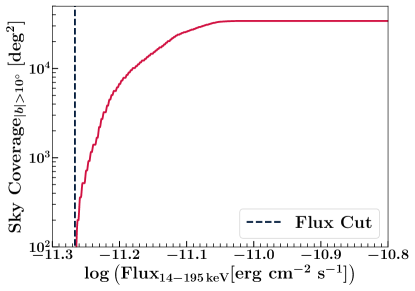
Figure 1: The Swift-BAT sky coverage for $|b|>10\degree$ and $5\sigma$ detection threshold, derived from Oh et al. (2018, see Section 2.2), rises from 300 deg² at the minimum sky coverage flux (blue dashed line) to 34,089 deg² above $F_{\rm 14-195\,keV}>10^{-11}\mbox{${\rm\,erg\,\,cm^{-2}\,s^{-1}}$}$.

Despite the BAT survey averaging over 9 years of observations, the sky coverage of the survey (i.e., how much time the instrument has looked at a particular position in the sky) is not perfectly uniform (see Oh et al., 2018). Hence the efficiency of the BAT instrument (i.e., the probability of detecting sources as a function of flux) changes depending on the chosen significance detection threshold. It is therefore paramount to know the sky coverage, $\omega(F)\equiv\omega(L,z)$, of the instrument, i.e., how the flux limit changes as a function of the surveyed sky solid angle ($\Omega$), given a significance threshold. This function is reported in Oh et al. (2018) for the whole sky for a significance threshold of $5\sigma$. In this work, in agreement with the chosen Galactic latitude and significance cuts (§ 2.1), we recalculate this function for $|b|>10\degree$ at $5\sigma$ threshold in the same way as described in Oh et al. (2018, see Figure 1). Sources with BAT flux $F_{\rm 14-195\,keV}>10^{-11}\mbox{${\rm\,erg\,\,cm^{-2}\,s^{-1}}$}$ are detected everywhere at $|b|>10\degree$ ($\Omega_{\rm max,|b|>10\degree}\sim 34,089$ deg²), while the available area decreases gradually toward lower fluxes, reaching $\sim 1\%$ of the surveyed area ($\Omega_{\rm min,|b|>10\degree}=300\,\rm deg^{2}$) at the limiting flux, $F_{\rm 14-195\,keV}\sim 5.4\times 10^{-12}\mbox{${\rm\,erg\,\,cm^{-2}\,s^{-1}}$}$.

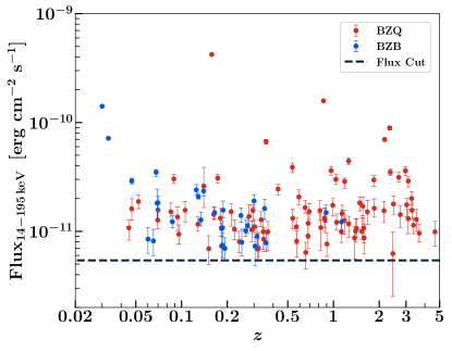
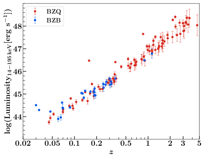
Figure 2: Left: Hard X-ray ($14-195\,\rm keV$) flux versus redshift for our clean sample of 118 blazars (see Section 2.2). The data points represent all identified blazars at $|b|>10\degree$ detected above $5\sigma$ with $F_{\rm 14-195\,keV}>5.4\times 10^{-12}\mbox{${\rm\,erg\,\,cm^{-2}\,s^{-1}}$}$ (dashed line) from the BAT 105 catalog: (red filled circles) BZQs, (blue filled circles) BZBs, including 3 BZGs and 1 BZU. Right: K-corrected hard X-ray ($14-195\,\rm keV$) luminosity as function of redshift for our clean sample.

2.3 Constructing the Blazar Sample

To avoid biases in the source selection, instead of relying directly on the BAT 105 classification, we performed a standard positional cross match between the list of 1069 sources (with counterpart positions taken from the BASS DR2 multi-wavelength catalog) and already existing blazar catalogs. These consist of the Roma-BZCAT (Massaro et al., 2015), the Combined Radio All-Sky Targeted Eight-GHz Survey (CRATES, Healey et al., 2007), the Candidate Gamma-Ray Blazar Survey Source Catalog (CGRaBS, Healey et al., 2008), the WISE Blazar-like Radio-Loud Source catalog (WIBRaLS, D’Abrusco et al., 2014) and the Fermi-LAT Fourth Source Catalog (4FGL, Abdollahi et al., 2020). Moreover, we checked the MOJAVE catalog (Lister et al., 2019) and a radio galaxy catalog (Yuan & Wang, 2012) for sources with small reported jet viewing angles, $\theta<5\degree$, which can therefore be classified as blazars. The positional cross match was done using the Sky with errors algorithm in TOPCAT; source coordinates and positional errors were taken from the respective catalogs. We consider blazars sources that have positional crossmatches with one or several of the above mentioned catalogs (i.e. within the 1$\sigma$ positional uncertainty, there was overlap between the catalog counterpart and the BAT source position). Our clean blazar sample contains 118 sources ($\sim 75\%$ of the total BAT 105 beamed AGN sample), 114 classified as BZQ, 33 as BZB, 10 as BZG, and 2 as BZU (Koss et al., 2017). We emphasize that these are the same 118 ‘beamed AGN’ found by applying Section 2.2 cuts to the total BAT-105 sample. The main properties of the clean sample are listed in Table 1. Figure 2 shows the distribution of sources flux (left panel) and K-corrected $14-195\,\rm keV$ luminosity (right panel) as a function of redshift.

To evaluate the incompleteness of the sample, we employ the zeroth-order assumption that uncertain sources (15 out of 1069, see Section 2.1) are distributed in type as the associated ones in the catalog. Since blazars represent 10% of the associated sources, we expect a 10% of the unassociated ones to be blazars, adding only one or two extra objects to our list. This incompleteness is completely negligible and of no impact for our results.

Table 1: Mean properties of clean blazar sample.

	Numbera	$<\Gamma_{\rm 14-195\,keV}>^{b}$	$<F_{\rm 14-195\,keV}>^{b}$	$<L_{\rm 14-195\,keV}>^{b}$	$z_{\rm min}^{c}$	$z_{\rm max}^{c}$
			$[$${\rm\,erg\,\,cm^{-2}\,s^{-1}}$$]$	$[\rm erg~{}s^{-1}]$
Total	118	$1.94\pm 0.47$	$2.31\times 10^{-11}$	$1.22\times 10^{46}$	0.03	4.65
BZQ	88	$1.82\pm 0.38$	$2.40\times 10^{-11}$	$2.75\times 10^{46}$	0.04	4.65
BZBd	30	$2.30\pm 0.51$	$2.06\times 10^{-11}$	$1.03\times 10^{45}$	0.03	1.13

3 The Luminosity Function

The luminosity function of a particular source class is defined as the number of objects per unit comoving volume ($dV$) and luminosity interval ($dL$). It can be written in its differential form as:

$$\phi(L,V(z))=\frac{d^{2}N}{dVdL}(L,V(z)).$$ (1)

The above can be interpreted as a function of redshift ($z$), adopting the transformation of comoving volume per unit redshift and solid angle ($dV/dzd\Omega$, see Hogg, 1999), as follows:

$$\phi(L,z)=\frac{d^{2}N}{dVdL}(L,V(z))\times\frac{dV}{dzd\Omega}.$$ (2)

Throughout this work, the luminosity labeled as $L$ indicates the $14-195\,\rm keV$ X-ray luminosity ($L\equiv L_{\rm X}$) derived using the flux and redshift information in the BAT 105 catalog. To calculate its evolution, it is custom to factorize $\phi(L,V(z))$ into a local luminosity function, $\phi(L,V(z=0))$, accompanied by an evolutionary factor, $e(z)$. For the purpose of our analysis, we adopt the notations and conventions detailed in Ajello et al. (2009, hereafter A09), Ajello et al. (2012b, hereafter A12) and Ajello et al. (2014, hereafter A14), which are here summarized.

The simplest parametrization for $\phi(L,V(z=0))$ is a straightforward power law

$$\begin{split}&\phi(L,V(z=0))=\frac{dN}{dL}=\frac{dN}{d\log L}\frac{d\log L}{dL}\\ &=\frac{A}{\ln(10)L}\left(\frac{L}{L_{*}}\right)^{-\gamma}=\frac{A}{\ln(10)L_{*}}\left(\frac{L}{L_{*}}\right)^{-\gamma^{\prime}},\\ \end{split}$$ (3)

where $L_{*}$ is a constant luminosity scale, fixed here to $10^{44}\,\rm erg~{}s^{-1}$, $A$ is the normalization factor and $\gamma$ the power-law index of the $dN/d\log L$, while $\gamma^{\prime}=\gamma+1$ is the power-law index of the $dN/dL$. Another envisaged scenario is a distribution described by a break occurring at some luminosity $L_{*}$, and it can be represented by a smoothly-joint broken power law of the form

$$\begin{split}\phi(L,V(z=0))&=\frac{A}{\ln(10)L}\left[\left(\frac{L}{L_{*}}\right)^{\gamma_{1}}+\left(\frac{L}{L_{*}}\right)^{\gamma_{2}}\right]^{-1}=\\ &=\frac{A}{\ln(10)L_{*}}\left[\left(\frac{L}{L_{*}}\right)^{\gamma_{1}^{\prime}}+\left(\frac{L}{L_{*}}\right)^{\gamma_{2}^{\prime}}\right]^{-1},\end{split}$$ (4)

where the $\gamma_{1}$ ($\gamma_{1}^{\prime}$) and $\gamma_{2}$ ($\gamma_{2}^{\prime}$) are respectively the low-end and high-end luminosity power-law indices of the $dN/d\log L$ ($dN/dL$), and $A$ the normalization.

As for the evolutionary properties of the blazar population, usually three scenarios are proposed: a pure luminosity evolution (PLE, i.e., sources are more/less luminous in the past, while their number density remains roughly constant), a pure density evolution (PDE, i.e., the number density of sources increases/decreases with redshift, but their typical luminosity remains constant) or a mixed luminosity-dependent density evolution (LDDE, i.e., sources density changes as a function of luminosity, which also varies as redshift increases). In the three different scenarios the evolved luminosity function translates as follows:

1. PLE:

   $$\phi(L,V(z))=\phi(L/e(z),V(z=0)),$$ (5)

2. PDE:

   $$\phi(L,V(z))=\phi(L,V(z=0))\times e(z),$$ (6)

3. LDDE:

   $$\phi(L,V(z))=\phi(L,V(z=0))\times e^{\prime}(z),$$ (7)

where the evolutionary factors are:

$$e(z)=(1+z)^{k}{\rm e}^{z/\xi},$$ (8)

with $z$ being the redshift, $k$ the redshift index and $\xi$ the evolutionary cut-off term; and

$$e^{\prime}(z)=\left[\left(\frac{1+z}{1+z_{C}(L)}\right)^{-p1}+\left(\frac{1+z}{1+z_{C}(L)}\right)^{-p2}\right]^{-1}$$ (9)

where $z_{C}(L)=z_{C}(L/10^{48.6})^{\rho}$, $z_{C}$ being the characteristic redshift; $p1$, $p2$ and $\rho$ are the redshift indeces.

In this work, we test all three different evolution scenarios. For the PDE and PLE we evaluate both the simple power-law and smooth broken power-law (Equation 3 and 4) shapes for the local luminosity function, $\phi(L,V(z=0))$. For clarity, the former is referred to as simple PDE/PLE (sPDE/sPLE), the latter as modified PDE/PLE (mPDE/mPLE) in the rest of the paper. For the LDDE case we only test the smooth broken power-law $\phi(L,V(z=0))$ (Equation 4).

3.1 Maximum-likelihood fit

In order to determine the best fit X-ray luminosity function (XLF) we follow the maximum likelihood (ML) method originally put forward by Marshall et al. (1983). The likelihood function is taken in its normalization-free form from Narumoto & Totani (2006) and can be written as

$$\mathcal{L}=\prod_{i=0}^{N_{\rm obs}}\frac{1}{N_{\rm exp}}\lambda(L_{i},z_{i}).$$ (10)

In the above, the product covers up to $N_{\rm obs}$, the total number of sources in the sample; $L_{i}$ and $z_{i}$ are the luminosity and redshift of the $i^{th}$ source and $\lambda(L,z)$ is defined as

$$\lambda(L,z)\equiv\phi(L,z)\omega(L,z),$$ (11)

where $\phi(L,z)$ is one of the luminosity function representations highlighted in the previous Section, and $\omega(L,z)$ is the sky coverage at a specific flux. Finally, $N_{\rm exp}$ is the expected number of observed sources for a particular $\phi(L,z)$ and is evaluated as:

$$N_{\rm exp}=\int_{z_{\rm min}}^{z_{\rm max}}\int_{L_{\rm min}}^{L_{\rm max}}\lambda(L,z)\frac{dV}{dzd\Omega}dLdz,$$ (12)

where the integrals limits are set to: $L_{\rm min}=10^{43}\,\rm erg~{}s^{-1}$, $L_{\rm max}=10^{50}\,\rm erg~{}s^{-1}$, $z_{\rm min}=0$, and $z_{\rm max}=6$. The minimum luminosity is chosen to be an order of magnitude lower than the minimum observed luminosity ($L_{\rm min,obs}\sim 10^{44}\,\rm erg~{}s^{-1}$). The maximum values of redshift ($z_{\rm max}$) and luminosity ($L_{\rm max}$) do not influence the fit results, hence they are arbitrarily set to the ones reported above. The standard $C=-2\ln(\mathcal{L})$ is then calculated as:

$$C=-2\left[\left(\sum_{i=0}^{N_{\rm obs}}\ln\lambda(L_{i},z_{i})\right)-N_{\rm obs}\ln\left(N_{\rm exp}\right)\right].$$ (13)

The free parameters in each representation of $\phi(L,z)$ are varied until the minimum value of $C$ is achieved, i.e., $\Delta C=1$ (under the limit for which $\mathcal{L}\propto\exp(-\chi^{2}/2)$, with $\chi^{2}$ following a chi-square distribution, see e.g., Loredo & Lamb, 1989). When the minimum is reached, the best-fit parameters and their associated $1\sigma$ errors are extracted (see Table 2). For the task we use the pyROOT implementation of Minuit. The Akaike Information Criteria (AIC, Akaike, 1974) is then employed to compare the different values of $C$ and determine the best-fit XLF model, ascribed to the lowest AIC value. The ML and AIC values are reported next to every tested model in Table 2 and we discuss the results in Section 4.

Table 2: Result of the maximum likelihood fit

SAMPLE

LF

Parameters

$C$

AIC

KSz

KSL

CXB %

Total

Aa

$\gamma$

k

$\xi$

sPLE

$1.14\pm 0.10$

$1.32\pm 0.08$

$1.87\pm 0.59$

$-2.98\pm 1.58$

1492.76

1500.76

0.10

0.31

2.89%

Aa

$\gamma$

k

$\xi$

sPDE

$1.57\pm 0.10$

$1.31\pm 0.08$

$4.13\pm 1.49$

$-1.28\pm 0.74$

1492.76

1500.76

0.10

0.31

2.89%

Aa

$L_{*}^{b}$

$\gamma_{1}$

$\gamma_{2}$

k

$\xi$

mPLE

$1.69\pm 0.15$

$1.47\pm 0.93$

$-0.51\pm 1.15$

$1.79\pm 0.19$

$2.79\pm 0.53$

$-2.23\pm 0.81$

1465.43

1477.43

0.92

0.43

4.21%

Aa

$L_{*}^{b}$

$\gamma_{1}$

$\gamma_{2}$

k

$\xi$

mPDE

$1.48\pm 0.13$

$1.50\pm 0.82$

$-0.70\pm 1.25$

$1.76\pm 0.17$

$7.74\pm 1.93$

$-0.78\pm 0.31$

1465.43

1477.85

0.96

0.44

19.58%

Aa

$L_{*}^{b}$

$\gamma_{1}$

$\gamma_{2}$

$p_{1}$

$p_{2}$

$z_{C}$

$\rho$

LDDE

$(1.92\pm 0.17)\times 10^{-9}$

$997.7\pm 733.8$

$0.79\pm 0.05$

$1.14\pm 0.19$

$4.75\pm 0.94$

$-1.44\pm 3.64$

$6.00\pm 3.82$

$0.27\pm 0.04$

1480.06

1496.06

0.73

0.39

0.08%

BZQ

Aa

$\gamma$

k

$\xi$

sPLE

$0.52\pm 0.05$

$1.36\pm 0.10$

$2.70\pm 0.61$

$-1.76\pm 0.62$

1293.84

1301.84

0.29

0.34

3.67%

Aa

$\gamma$

k

$\xi$

sPDE

$0.52\pm 0.05$

$1.35\pm 0.10$

$6.38\pm 1.64$

$-0.74\pm 0.28$

1293.84

1301.84

0.29

0.34

3.65%

Aa

$L_{*}^{b}$

$\gamma_{1}$

$\gamma_{2}$

k

$\xi$

mPLE

$1.13\pm 0.12$

$1.01\pm 0.66$

$-1.00\pm 2.07$

$1.67\pm 0.17$

$3.23\pm 0.57$

${-1.62\pm 0.47}$

1281.87

1293.87

1.00

0.45

2.55%

Aa

$L_{*}^{b}$

$\gamma_{1}$

$\gamma_{2}$

k

$\xi$

mPDE

$0.89\pm 0.09$

$1.15\pm 0.83$

$-0.88\pm 2.02$

$1.66\pm 0.17$

$8.60\pm 2.00$

$-0.60\pm 0.09$

1281.94

1293.94

1.00

0.45

10.35%

Aa

$L_{*}^{b}$

$\gamma_{1}$

$\gamma_{2}$

$p_{1}$

$p_{2}$

$z_{C}$

$\rho$

LDDE

$(7.7\pm 0.82)\times 10^{-5}$

$1.55\pm 1.93$

$-3.48\pm 1.98$

$1.55\pm 0.19$

$4.54\pm 0.99$

$-9.43\pm 11.03$

$3.61\pm 0.36$

$(2.356.08\times 10^{-8})\pm 0.03$

1281.10

1297.10

0.99

0.44

4.38%

3.2 Consistency tests

To test the consistency of our results, we further performs two checks:

1. The Kolmogorov-Smirnov (KS) test. Given a empirical distribution function and a cumulative one (derived from the representative model), the test returns the probability that the data and the model are drawn from the same distribution. If the probability is too low (the threshold is here set to KS$<30\%$), the model can be disregarded. This is applied to both the redshift (KS_z) and luminosity (KS_L) distributions of our blazar sample.

2. The source count distribution (logN-logS). For any luminosity function, the number of expected sources as a function of flux ($S$) can be computed as:

   $$N(>S)=4\pi\int_{0}^{z_{\rm max}}\int_{L(z,S)}^{\infty}\phi(L,z)\frac{dV}{dzd\Omega}dLdz.$$ (14)

   The prediction is then compared to the observed logN-logS

   $$N(>S)=\sum_{i=0}^{N_{\rm obs}}\frac{1}{\omega(S_{i})}\quad S_{i}>S,$$ (15)

   where the above sum covers up to the the total number of observed sources ($N_{\rm obs}$) and $\omega(S_{i})$ is the sky coverage evaluated at the flux of the $i^{th}$ source ($S_{i}$). Importantly, the bright-end slope of the logN-logS can also inform us about the evolution of the population. In a Euclidian space, if there was no evolution, a source class of a given luminosity would be distributed according to $N(>S)\propto S^{-3/2}$. If instead the considered class of objects underwent a positive (negative) evolution, the slope of the logN-logS would be greater (lesser) than 1.5.

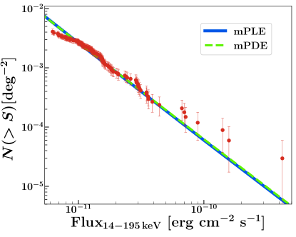
Figure 3: Cumulative BAT-blazars logN-logS, i.e., total number of sources above a certain flux corrected for the survey sky coverage $\omega(S)$, $N(>S)$, as a function flux (Eq. 14-15). The observed logN-logS is represented by the red data points, while the blue solid and green dashed lines show the prediction from the best-fit mPLE and mPDE models, respectively. We note that in this representation the data points are not independent from one another. As can be seen, both models explain reasonably well the observed distribution in the region $8\times 10^{-12}\,\rm erg~{}cm^{-2}~{}s^{-1}$ to $10^{-10}\,\rm erg~{}cm^{-2}~{}s^{-1}$, where most source counts lie. As detailed in Appendix A, the slight discrepancy between the data and the model predictions below $8\times 10^{-12}\,\rm erg~{}cm^{-2}~{}s^{-1}$ does not influence the validity of our results. The derived spectral slope for the logN-logS is $1.62\pm 0.05$, indicative of a positive evolution of this source class (see § 3.2)

.

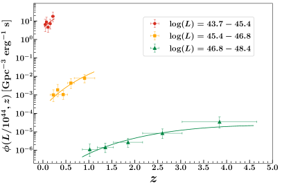
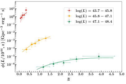
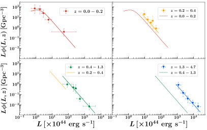
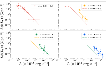
Figure 4: Total blazar (left) and FSRQs (right) X-ray luminosity function, $\phi(L,z)$ (where $L\equiv L_{\rm X}$). On the top panels, it is shown as function of redshift in various luminosity bins; in the bottom panel it is shown are function of luminosity at different redshift bins. The data points are the one deconvolved via the $N^{\rm obs}/N^{\rm mdl}$ method described in Section 4.1. The solid lines instead show our best-fit mPLE model. In the bottom panels, to highlight the evolution at different luminosities, the XLF from the previous redshift bin is overplotted with dashed lines.

4 Best-fit Luminosity Function

4.1 All blazars

The results from the ML fit are three-fold. Firstly, as can be noted in Table 2, the use of a smooth broken power law to represent the local luminosity function greatly improves the fit results with respect to the simpler power-law case ($\Delta_{\rm AIC,sPLE-mPLE}\sim 23$). The KS statistics values also show that the latter models are close or below the 30% threshold set in Section 3.2, hence can be disregarded. This outcome was already noted in A09, where the authors emphasize how it is necessary to introduce a luminosity break to explain the observed redshift and luminosity distribution.

The second result is that it is not possible to distinguish between the luminosity evolution or the density evolution scenarios. This is hinted in the simple power-law scenario and confirmed by the broken power-law one. In fact, results on the ML fit and AIC values between sPDE/sPLE and mPDE/mPLE only slightly differ ($\Delta_{\rm AIC,mPDE-mPLE}\sim 0.4$), rendering the models comparable to each other. Moreover, the LDDE case does not improve the results upon either the mPDE or the mPLE. Indeed, both ML fit and AIC values are higher than the mPDE/mPLE cases ($\Delta_{\rm AIC,LDDE-mPLE}\sim 19$), and the best-fit redshift index is close to zero ($\rho=0.27\pm 0.04$), therefore removing the luminosity dependence from Equation 9.

Finally, the evolutionary parameters confirm a positive evolution of the blazars population ($k>2$) both for the mPDE and mPLE case. The evolutive parameter $\xi$ is coherently negative for both cases, indicating an exponential cut-off at high redshifts. Moreover, the slope derived from our best-fit luminosity function to the logN-logS (shown in Figure 3) is $1.62\pm 0.05$ for both the mPLE/mPDE results, in accordance with a positive evolution of the source population, a result already emphasized by A09.

The best-fit index value of the distribution for the sPLE/sPDE is $\gamma=1.31\pm 0.08$. This is significantly ($\sim 3\sigma$) harder than the one reported A09 for the sPDE model ($\gamma_{\rm A09}=1.67\pm 0.13$), though in agreement with their adopted sPLE one ($\gamma_{\rm A09}=1.26\pm 0.07$, see Table 4 of A09). For the mPDE/mPLE scenarios, the bright-end slopes of the distribution are softer with respect to the sPDE/sPLE ones, i.e., $\gamma_{2}=1.79\pm 0.19$. It is important to note that these values are in very good agreement with the indices reported by A09 in the simple power-law scenario, and similar to the one found for the evolution of the unbeamed jetted AGN population ($\gamma_{\rm FRII,15GHz}\sim 1.65$, Cara & Lister, 2008, see Section 8). On the other hand, there is a difference at the $\sim 3\sigma$ level from the values found in A09 for the mPLE ($\gamma_{2,\rm A09}=2.73\pm 0.37$) and mPDE ($\gamma_{2,A09}=2.54\pm 0.21$) cases . We note that this discrepancy can be accounted for the fact that our sample (1) reaches higher redshifts, (2) has three time the source number than the one used by A09, and (3) goes almost an order of magnitude deeper in flux. It follows that our fit is able to more accurately constrain the shape of these distributions. The faint-end slope is flat ($\gamma_{1}<1$) for both mPLE/mPDE, although poorly constrained due to the absence of sources. A flattening of the luminosity function is expected at low luminosities as a result of beaming (Urry & Shafer, 1984), with a predicted spectral index value between 1 to 1.5. Our derived $\gamma_{1}$ fit values are consistent with this slope, taking into account the errors.

In Figure 4 the LF prediction from the mPLE best-fit model are shown, as function of redshift in the top left and as function of $14-195\,\rm keV$ luminosity in the bottom left panel. The displayed data points are the deconvolved ones, obtained by calculating the scaling factor through the ${N^{\rm obs}}/{N^{\rm mdl}}$ technique. This has been shown to be an effective unbiased representation for any predicted LF given the real data (see La Franca & Cristiani, 1997; Page & Carrera, 2000; Miyaji et al., 2001), which are unfolded as such:

$$\phi(L,z)^{\rm obs}=\phi(L,z)^{\rm mdl}\times\frac{N^{\rm obs}}{N^{\rm mdl}},$$ (16)

where

$$\frac{N^{\rm obs}}{N^{\rm mdl}}=\frac{N^{\rm obs}(L_{i},z_{i})}{\int_{z_{\rm min}}^{z_{\rm max}}\int_{L_{\min}}^{L_{\rm max}}dLdz\lambda(L,z)},$$ (17)

and $N^{\rm obs}$ is the observed number of blazars, while $N^{\rm mdl}$ is the number predicted to be observed given $\phi(L,z)$. We stress that the mPDE results look formally identical to the mPLE ones in this representation. In fact, it is clear that the XLF data as function of luminosity are distributed accordingly to a straight power law (in $\log-\log$ space) without any apparent turnover, which impedes the differentiation between a luminosity versus a density evolution scenario. This behavior, discussed further in Section 7, is reflective of the fact that the BAT is sampling the high-luminosity tip of the blazar population, and it is still not able to detect the break (except maybe at the lowest redshift, see below) in the luminosity function expected as a result of beaming. The mPLE or mPDE models are favored by the ML fit, indicating that indeed a break and a change in slope of the distribution are preferred. This not only is expected as a direct consequence of beaming, but also because if the distribution was a continuing straight power law, the hard X-ray sky would be dominated by too many low-luminosity blazars. In Figure 4, it can be noticed from the model prediction that the break in luminosity should start appearing in the lowest redshift bin ($z=[0.0,0.2]$). Nevertheless, the statistical uncertainties on the data do not allow us to see the break with high significance. In fact, mPLE and mPDE are still not differentiable in likelihood values as they are sampling a power-law distribution with a luminosity cut-off occurring at the minimum observed luminosity ($L_{*}\sim 10^{44}\,\rm erg~{}s^{-1}$), and hence are formally identical to each other (Bahcall, 1977).

4.2 FSRQs

FSRQs outnumber BL Lacs in our sample ($75\%$ of the total, see Table 1); they also are more luminous, and have better constrained redshifts which span a larger range (the farthest source being at $z=4.65$, see Table 1). To test their evolution, we fitted the same models as the ones used for the overall population. Results show that FSRQs drive the evolution of the whole BAT-blazar sample. Their XLF is similarly well described by a broken power law with a luminosity cut-off occurring at $L_{*}\sim 10^{44}\mbox{${\rm\,erg\,\,cm^{-2}\,s^{-1}}$}$. Both the mPDE/mPLE shapes give consistent fits, with the high-end slope being $\gamma_{2}=1.67\pm 0.17$. It is interesting to note that the results on the indices on the $\phi(L,V(z=0))$ are very similar to the ones reported on the LAT FSRQs studied in A12 (where $\gamma_{2,\rm 100\,MeV-100\,GeV}=1.60$, see Table 3 in their work). The mPLE representation is shown on the right panels of Figure 4, and Figure 5 displays the number density of these sources as a function of redshift.

As previous works have found, this class of objects evolve positively in redshift ($k=5.05\pm 0.79$, i.e., their number density or luminosity increases as function of redshift), although uncertainties on the evolutionary parameters remain quite high. This positive evolution is also confirmed by the slope of the logN-logS derived from the best-fit luminosity function which is $1.60\pm 0.07$ for both the mPLE/mPDE models. The factor $e(z)$ (Equation 8) allows us to estimate the peak of the distribution, which occurs at $z_{\rm peak}=-1-k\xi$. Given the best-fit values of these parameters, the peak is located at $z_{\rm peak}\sim 4.3$. Nevertheless, the errors associated with $k$ and $\xi$ allow for this value to range between $z_{\rm peak}\in[3.5,5.5]$, impeding the exact localization of the maximum of this population of powerful jetted AGN.

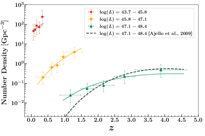
Figure 5: Number density plot of BAT FSQRs as function of redshift and luminosity bins. The data points are the one deconvolved via the $N^{\rm obs}/N^{\rm mdl}$ method and the solid lines show the best-fit mPLE model. For comparison, number densities model prediction from A09 in the highest luminosity bin are shown ($\log L=47.1-48.4\,\rm[erg~{}s^{-1}]$, black dotted line). It can be seen how our best-fit XLF predicts a different XLF shape implying fewer sources at the highest redshifts, $z=[3-5]$.

We stress that for the first time our BAT-blazar sample contains one source that lies beyond $z=4$ (SWIFT 1430.6+4211, BAT index 1448). This enables us to set more solid constraints on the location of the peak, and to assess whether a turnover in the luminosity function of the most luminous sources is starting to appear in the data. As evident from Figure 4 (top right panel), even for the high-luminosity end of the population, a turnover of the XLF remains undetected, placing the cut-off peak beyond $z=4$.

To further assess the likelihood that the peak lies at $z>4$ (or viceversa), we perform ML fits using the mPDE evolutionary model, forcing the peak to occur at a specific redshift in the range $z_{\rm peak}=[3,5]$. Figure 6 shows the results of ML values as a function of $z_{\rm peak}$. It can be seen that our fits support the scenario in which $z_{\rm peak}\sim 4.3-4.4$ ($C$ is at a minimum) and could occur even at $4.6$, the maximum redshift of our sample. Instead, below $z<4$ results differ significantly from the minimum ML values, excluding the possibility of the peak occurring at later cosmic times. It is therefore with high confidence that we ascertain that the peak lies $z\geq 4$, confirming the results found by A09. A deeper all-sky X-ray survey would most likely be necessary to pinpoint this peak.

Figure 5 shows the number density of FSRQs as function of redshift for different luminosity bins predicted by the mPLE best-fit. The data points are derived using the $N^{\rm obs}/N^{\rm mdl}$ technique. For comparison, the model prediction on FSRQ number densities derived from the MPLE best-fit reported in A09 in the highest luminosity bin are plotted ($\log(L)=47.1-48.4$, black dotted line). It can be seen how our best-fit model predicts lower number densities than A09 (e.g., two times fewer sources per comoving volume at $z=4$), implying the existence of fewer highly luminous FSRQs than previously anticipated.

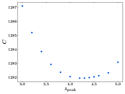
Figure 6: Log-likelihood results ($C$, see Equation 13) for the BAT FSRQs using the MPDE model fixing the position of the $z_{\rm peak}=[3,5]$. It can be noticed how the fit values reach a minimum for a peak occurring at $z_{\rm peak}=4.3-4.4$, confirming that the luminous BAT FSRQ population peaks at $z>4$.

5 Average blazar SED

The high-energy (hard X- to $\gamma$-rays) blazars SED typically shows a double power-law shape with a peak located in the MeV to GeV range (depending on the source class and luminosity, Ghisellini et al., 1998, 2017, e.g.,). Here we aim to phenomenologically characterize such high-energy SED in order to correctly account for their spectral shape in the whole $14\rm\,keV-10\rm\,GeV$ range. This in turn allows us to extrapolate their contribution to the CXB as well as making prediction for the MeV background. We choose to consider only the sources belonging to the FSRQ class, as they are the dominating population (in luminosity) in our sample, and are expected to produce the higher contribution to the CXB (see A09).

5.1 LAT detected BAT FSRQs

At first, we restrict ourselves to the sources which have both BAT and LAT data. This results in 46 objects (out of 88 BAT FSRQs). The chosen putative SED spectral shape is the following:

$$E^{2}\frac{dN}{dE}=E^{2}\left\{K\left[\left(\frac{E}{E_{b}}\right)^{\eta_{1}}+\left(\frac{E}{E_{b}}\right)^{\eta_{2}}\right]^{-1}\right\},$$ (18)

where K is the normalization constant, $E_{b}$ is the break position in the distribution, and $\eta_{1}$ and $\eta_{2}$ are the low-energy and high-energy spectral indices, respectively. In A12, the contribution from the extragalactic background light (EBL, Fermi-LAT Collaboration et al., 2018b) was added to the same framework as an exponential cut-off to Equation 18. Since the contribution of the EBL is significant at $>10\,\rm GeV$, far from the background energies of interest to this work, we limit the fit to $<10\,\rm GeV$ and we avoid adding the EBL contribution. The luminosity-dependent SEDs are obtained by multiplying both sides of Equation 18 by $4\pi D_{L}(z)^{2}$, with $D_{L}$ being the luminosity distance of the source (Hogg, 1999), and all SEDs are shifted by $(1+z)$ in order to transform to the source rest-frame. The hard X-ray and $\gamma$-ray spectra of the sources are obtained considering a power-law spectral shape in both bands, using the flux and index values from the BAT 105 catalog and the 4FGL, respectively. The $1\sigma$ uncertainties in the spectra are accounted for by a bowtie spectrum using both flux and index error values provided by the two catalogs. We fit Equation 18 simultaneously to both BAT and LAT data and derive the best-fit parameters for every source using a standard minimizing $\chi^{2}$ technique. In turn, this allows us to divide the sample in different luminosity bins, chosen such that they contain roughly the same number of sources.

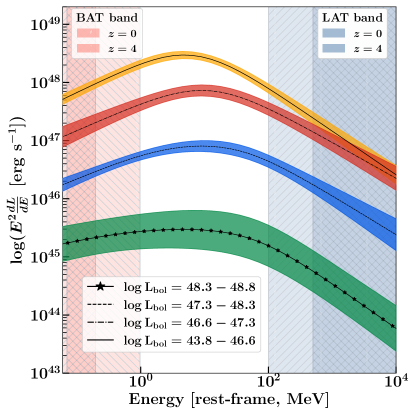
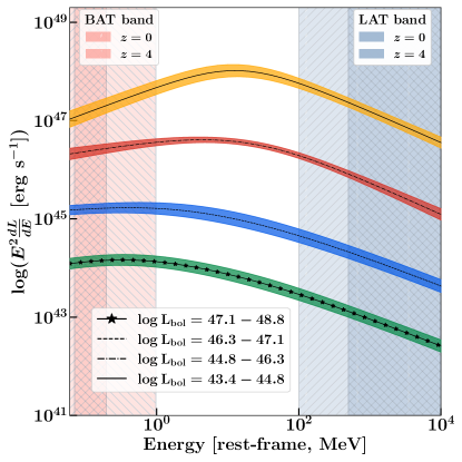
Figure 7: Average high-energy SED of the FSRQs in our sample derived by fitting: (i) only sources which are BAT and LAT detected (46 sources, left panel) and (ii) the whole sample (88 sources, right panel). The details of the fits can be found in Section 5. The different lines represent the mean of the distribution at different luminosity bins (as labelled in the Figure). The errors (shown as colored shaded regions) are derived employing a Jackknife technique. The high-energy SED spectral form does not show strong dependence of the chosen luminosity bin. On the right panel it can be noticed that the lowest luminosity sources have on average an SED peaking at lower energies ($\sim 3\,\rm MeV$ versus $\sim 17\,\rm MeV$ for the highest luminosity sources). This relation between the energy break position and the source luminosity has been calibrated (see Section 5.2 and Figure 8, right) in order to properly take into account the contribution to the MeV background. The shaded hatched pink and light blue regions represent the BAT and LAT energy bands, respectively, shifted for sources at $z=0$ (forward slash) and $z=4$ (backward slash). As can be seen, the MeV peak of the sources falls exactly in the region which still remains uncovered by both instruments and is critical to determine the entire SED.

The binned luminosity SEDs are shown in Figure 7 (left panel). The errors are computed using the Jackknife method (Efron & Stein, 1981). As can be seen, the shape of the FSRQs SED does not show a strong evolution in luminosity, i.e., both the break position and the spectral indices are very similar in every luminosity bin. This was already noted by previous works and is in contrast with the anti-correlation between the source luminosity and the low-energy synchrotron peak (see A09, Ghisellini, 2010; Ghisellini et al., 2017; Paliya et al., 2019). Importantly, it allows us to establish average SED parameters for these sources, which result to be: $\eta_{1}=1.53\pm 0.09$, $\eta_{2}=2.65\pm 0.07$ and $E_{b,\rm rest-frame}=16.70\pm 1.82\,\rm MeV$. To further check for consistency, we extract the values of spectral indices and energy break from the average blazar SED models reported in Paliya et al. (2019). This results in $\eta_{1}\sim 1.45-1.60$, $\eta_{2}\sim 2.45-2.63$ and $E_{b,\rm rest-frame}\sim 9-12\,\rm MeV$, values that are in complete agreement with our fits. In Figure 7, the shaded hatched pink and light-blue regions display the BAT and LAT energy bands, respectively, shifted for sources at $z=0$ (forward slash) and $z=4$ (backward slash). As can be seen, the MeV peak of the sources falls exactly in the region which still remains uncovered by both instruments and would be critical to determine the full SED.

5.2 LAT-undetected BAT FSRQs

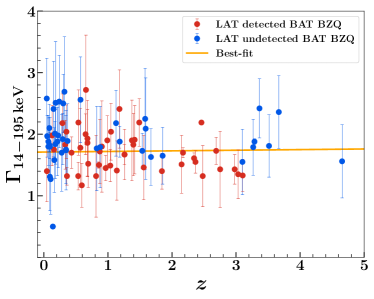
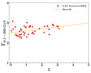
Figure 8: Left: BAT ($14-195\,\rm keV$) photon index versus redshift of all BAT FSRQs in our sample. Red data points represent LAT-detected sources, while blue data points are the LAT-undetected ones. The yellow line is the best-fit linear relationship calculated for these data. The slope is very flat ($m_{\rm BAT}=0.01\pm 0.01$) indicating that there is no evolution in redshift of the BAT photon index, and the intercept values gives us the average value of $c_{\rm BAT}=1.71\pm 0.01$. Right: LAT ($0.1-300\,\rm GeV$) photon index versus redshift of all LAT-detected BAT FSRQs in our sample (red data points). The best-fit line is shown in yellow. Similarly to the BAT regime, the slope is very flat ($m_{\rm LAT}=0.09\pm 0.03$) and the intercept returns an average photon index $c_{\rm LAT}=2.48\pm 0.05$. These empirical relations confirm that there is no dependence in redshift of the high-energy SED spectral slopes of BAT FSRQs.

In order to understand whether the LAT-undetected blazars would influence the above result, we tried establishing an average $14\,\rm keV$ to $10\,\rm GeV$ SED for these sources. We note that there is neither a redshift nor a X-ray luminosity dependence between LAT-detected and -undetected blazars for our BAT-selected sample, i.e. LAT-undetected sources lie in the same luminosity-redshift space as the LAT-detected ones.

As results in Section 5.1 point to the non-evolution of the average blazar SED with luminosity, we wished to understand if this was consistent with the data. Therefore, we perform (i) a linear fit between the BAT ($14-195\,\rm keV$) photon index and redshift of all BAT FSRQs and (ii) a linear fit between the LAT ($0.1-300\,\rm GeV$) photon index and redshift of all BAT FSRQs detected by the LAT. In agreement with the results in Section 5.1, both fits return very flat slopes ($m_{\rm BAT}=0.01\pm 0.01$ and $m_{\rm LAT}=0.09\pm 0.03$) and there is no statistically significant difference between a linear or a constant behavior in redshift (i.e. $m=0$); therefore there is no dependence in redshift of either the BAT or LAT photon indices. In the hard X-ray regime, the best-fit value for the intercept is $c_{\rm BAT}=1.71\pm 0.01$, and in the $\gamma$-ray regime $c_{\rm LAT}=2.48\pm 0.05$. Figure 8 shows these results. The value of the BAT intercept is softer with respect to the best-fit average spectral index from the LAT-BAT SED ($c_{\rm BAT}=1.71$ vs. $\eta_{1}=1.53$). This behaviour is mostly influenced by the low-$z$ (low-luminosity) sources that are LAT-undetected (upper left corner of Figure 8, left panel), and it is indicative of the fact that for these objects the BAT is sampling the SED closer to the high-energy peak, resulting in a softer photon index. With these relations in hand, we can assign a $\gamma$-ray spectral slope to all LAT-undetected FSRQs, knowing their redshift. For each source that is undetected by the LAT, we assign a $\gamma$-ray flux that does not violate the 12-year upper limits computed at the position of that source. The mock $14\,\rm keV$ to $10\,\rm GeV$ SED of the LAT-undetected sources is therefore constructed using BAT real data and LAT upper limits.

We employ the same formalism as Section 5.1 to derive the average SED using the total sample of 88 blazars. The result is shown in Figure 7 (right panel). Overall the average SED shape is similar to what found in Section 5.1, and the best-fit average spectral slopes are $\eta_{1}=1.70\pm 0.14$, $\eta_{2}=2.61\pm 0.03$. Interestingly, it can be seen that as the luminosity decreases, the peak position shifts slightly towards lower energies ($E_{\rm b,rest-frame}\sim 3\,\rm MeV$ for the lowest luminosity bin versus $E_{\rm b,rest-frame}\sim 17\,\rm MeV$ for the highest luminosity bin). This finding is closely related to the softer photon index detected by the BAT for the low-$z$ (low-luminosity) sources and it can be explained by the fact that the lower luminosity FSRQs have on average lower Doppler factors, making them less luminous and more low-energy peaked (see also Section 7.1, e.g. Ghisellini, 2015; Sbarrato et al., 2015). We take into account the shift of the SED to lower energies at lower luminosities (as in Figure 7, right) using $\log{E_{b,\rm rest-frame}[\rm MeV]}=0.35\times\log{L_{\rm BAT}-15.44}$ to estimate the contribution of blazars to the MeV background.

6 Contribution to the high-energy Backgrounds

Resolving the CXB in its different components has so far been a challenge. Although above 10 keV low-luminosity, unbeamed AGNs are expected to contribute the most to the CXB (e.g., Ajello et al., 2012a; Ueda et al., 2014; Aird et al., 2015; Ananna et al., 2019), blazars have been predicted to account up to $\sim 10-20\%$ of it in the hard X-ray band covered by BAT ($14-195\rm\,keV$, e.g., A09). With the best-fit blazar X-ray luminosity function in hand, it is possible to infer the contribution of the blazar population, and in particular of FSRQ one, to the total CXB. We calculate this contribution as follows:

$$\begin{split}&F_{\rm CXB_{\rm 14-195\,\rm keV}}=\int_{V_{\rm min}}^{V_{\rm max}}\int_{L_{\rm min}}^{L_{\rm max}}dV^{\prime}dL^{\prime}F(L^{\prime},z^{\prime})\phi(L^{\prime},z^{\prime})\\ &=\int_{z_{\rm min}}^{z_{\rm max}}\int_{L_{\rm min}}^{L_{\rm max}}dz^{\prime}dL^{\prime}\frac{dV}{dz^{\prime}d\Omega}F(L,z^{\prime})\phi(L^{\prime},z^{\prime})\end{split}$$ (19)

where $F(L,z)$ is the flux of a source with luminosity $L$ at redshift $z$ and $\phi(L,z)$ is the best-fit XLF. The limits on the integral are: $z_{\rm min}=0$ , $z_{\rm max}=6$, $L_{\rm min}=10^{43}\,\rm erg~{}s^{-1}$ and $L_{\rm max}=10^{50}\,\rm erg~{}s^{-1}$.

The results for the various background contribution are as follows. For the mPLE model: $F_{\rm CXB_{\rm 14-195\,\rm keV},ALL}=6.5\times 10^{-9}\,\rm erg~{}cm^{-2}~{}s^{-1}~{}sr^{-1}$, $F_{\rm CXB_{\rm 14-195\,\rm keV},FSRQ}=3.5\times 10^{-9}\,\rm erg~{}cm^{-2}~{}s^{-1}~{}sr^{-1}$. For the mPDE model: $F_{\rm CXB_{\rm 14-195\,\rm keV},ALL}=2.78\times 10^{-8}\,\rm erg~{}cm^{-2}~{}s^{-1}~{}sr^{-1}$, $F_{\rm CXB_{\rm 14-195\,\rm keV},FSRQ}=1.5\times 10^{-8}\,\rm erg~{}cm^{-2}~{}s^{-1}~{}sr^{-1}$. The intensity on the CXB in the $14-195\,\rm keV$ as measured by Ajello et al. (2008) is $I_{\rm CXB,14-195\,\rm keV}=1.5\times 10^{-7}\,\rm erg~{}cm^{-2}~{}s^{-1}~{}sr^{-1}$. It follows that, employing the mPLE model, the BAT blazars contribute $\sim 4\%$ to this background, while the mPDE predicts a $\sim 19\%$ contribution. If we consider FSRQs alone, the values are, respectively, $\sim 2\%$ and $\sim 10\%$. It is obvious that, although their contribution is non zero, BAT blazars are not the dominant source class that can account for the whole CXB in the $14-195\,\rm keV$ regime, confirming A09 results.

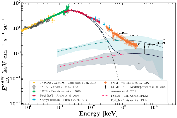
Figure 9: Intensity spectrum of the CXB and derived contribution of the FSRQs using the best fit mPLE model (pink dash-dotted line and gray shaded region) and the mPDE one (light blue dash-dotted line and cyan shaded region). The data points represent the different measurements of the cosmic diffuse background, and have been extracted from the works indicated in the label (Fukada et al., 1975; Gendreau et al., 1995; Watanabe et al., 1997; Weidenspointner et al., 2000; Revnivtsev et al., 2003; Ajello et al., 2008; Cappelluti et al., 2017). The dashed black line is the model prediction of the total contribution of AGNs to the CXB as derived by Ananna et al. (2019). The solid black and gray lines represent the sum of the total contribution from AGNs and FSRQs using the mPLE and mPDE models, respectively. The spectrum of FSRQs has been taken from the best-fit SED derived in Section 5. The shaded areas are derived from Monte Carlo simulations employing the best-fit parameter ranges.

In Figure 9 we show the intensity spectrum of the cosmic high-energy background (from $\sim 0.5\,\rm keV$ to $\sim 30\,\rm MeV$) and the predicted contribution of FSRQs from $14\,\rm keV$ to $30\,\rm MeV$, employing the best-fit mPLE and mPDE models. We adopt Equation 19 and the spectral shape derived from Section 5.2 to extrapolate the blazar contribution to the MeV regime, where $F(L,z)$ becomes $F(L,z,E)$, hence introducing the dependence on the blazar spectrum. The position of the blazar SED energy break ($E_{b,\rm rest-frame}$, Eq. 18) is allowed to vary depending on the luminosity, following the results of Section 5.2. The $1\sigma$ uncertainty range (shaded gray/light blue areas in Figure 9) is calculated through a Monte Carlo approach, producing realization of the luminosity function $\phi(L,z)$ that take into account the errors associated with the best-fit parameters. It can be seen how, although in the BAT regime FSRQs are subdominant, conversely in the $>500\,\rm keV$ regime their contribution is sufficient to explain the entire MeV background ($0.5-30\rm\,MeV$). It is important to note how the mPLE model can explain $\sim 50-70\%$ of the MeV background above $1\,\rm MeV$. On the other hand, the mPDE model slightly over-predicts the MeV background above few $\rm MeV$, although the $1\sigma$ uncertainty band is quite large in this energy range. It needs to be pointed out that other source classes have been anticipated to non negligibly contribute in this band. For example, supernovae could contribute $\sim 10-30\%$ to the MeV background (e.g., Iwabuchi & Kumagai, 2001; Ruiz-Lapuente et al., 2016). This hints to the fact that the mPLE model is preferred with respect to the mPDE one. As highlighted by Figure 9, the mPLE extrapolation to MeV energies allows for contribution from other source classes.

Furthermore, to check whether our prediction of the blazar contribution well fits within population synthesis studies of other AGN classes, we also consider the contribution of AGNs to the CXB recently derived by Ananna et al. (2019). The black and gray solid lines in Figure 9 represent the total model contribution of the two classes of sources. It can be noted that between $100\,\rm keV<E<500\,\rm keV$, added contributions of AGN and blazars undergoing a mPLE evolution fall short of completely explaining the background. Conversely, if we employed the mPDE model, we could easily recover this gap though over predicting the MeV regime. Nevertheless, we caution that uncertainties in the $100-1000\,\rm keV$ range ascribed to (i) the measurements of the background, (ii) models of non-jetted AGN components that could contribute in this regime (e.g., shape of the X-ray corona, Inoue et al., 2008; Fabian et al., 2015), and (iii) the extrapolation of the blazar model distributions, could naturally account for the discrepancy.

Recent work from Toda et al. (2020) predicts that the maximum contribution from FSRQs to the MeV background is $\sim 3\%$. In their work, the authors perform the study with 53 BAT FSRQ (vs. 88 in this work) and they do not recalculate the sky coverage (which could lead to biases in the results, see Section 2.2) but use the all-sky one from Oh et al. (2018). Moreover, they work under the assumption that this source class follows a LDDE evolutionary paradigm. As derived from our fits (Section 4), this (more complex) modelling is not significantly required from our data, as indicated by the fact that the luminosity dependence on the redshift evolution is compatible with zero. Moreover, we note that the spectral indices of the XLF derived for the LDDE scenario ($\gamma_{1}=-3.41\pm 1.98$ and $\gamma_{2}=1.55\pm 0.19$, Table 2) are compatible with the mPDE/mPLE ones (within the statistical uncertainty), further emphasizing how these models are yet to be disentangled for this population. Finally, complexities of the sky coverage and sensitivity may lead to divergent results from their work to ours.

7 Distribution of jet properties

Significant selection effects have to be considered when dealing with relativistically beamed source emission. Indeed, Doppler effects can both enhance or de-boost the intrinsic jet emission by hundreds if not thousand of times (e.g., Kellermann et al., 2003; Ghisellini et al., 2017; Yuan et al., 2018; Lister et al., 2019). On the other hand, it is possible to obtain information about the parent population taking into account the same beaming effects. The observed luminosity $L$ from a highly beamed relativistic source is related to its intrinsic (unbeamed) luminosity $\mathscr{L}$ by

$$L=\delta^{p}\mathscr{L},$$ (20)

where $\delta$ is the kinematic Doppler factor

$$\delta=\frac{1}{\Gamma(1-\beta\cos\theta)}.$$ (21)

In the above, $\Gamma$ is the Lorentz factor of the jet, i.e., how fast are the electron moving along the structure (i.e. what is they bulk flow motion); it is related to the velocity of the emitting plasma $\beta=v/c$ by $\Gamma=1/\sqrt{(1-\beta^{2})}$, where $c$ is the speed of light. The power $p$ depends both on the radiation emission processes at the considered frequencies and on the jet configuration. In the hard X-ray regime covered by BAT, blazar SEDs are in general dominated by the rising non-thermal power law, a result of inverse Compton scattering experienced by the electrons in the jet. The relativistic particles could be interacting with the same photons they produced once accelerated via synchrotron process, hence boosting them in a synchrotron self Compton scenario (SSC, e.g., Ghisellini & Maraschi, 1989); it is also expected that photon fields external to the jet are enhanced by these same electrons via external Compton process (EC, e.g., Sikora et al., 1994). In Dermer (1995) relationships between observed flux density and powers of the kinematic Doppler factor are provided for the EC and SSC cases; for the EC $p=4+2\alpha$ and for the SSC $p=3+\alpha$, where $\alpha$ is the source spectral index.

Another factor that has to be taken into account is how beaming alters the shape of the intrinsic luminosity function. Urry & Shafer (1984) solved this problem for the case where the intrinsic luminosity function, $\phi(\mathscr{L})$, starts off as a simple power law of the form:

$$\phi(\mathscr{L})=k_{1}\mathscr{L}^{-B},$$ (22)

where $B$ is the index of the distribution, and $k_{1}$ the normalization. Under the assumption that the jets orientation are distributed uniformly, $P_{\theta}(\theta)\propto\sin\theta$, and that the plasma moves along the jet with a single $\Gamma$ value, $P_{\Gamma}(\Gamma)\propto\delta(\Gamma-\Gamma_{0})$, Urry & Shafer (1984) showed that the observed luminosity function, $\phi(L)$, just by the act of beaming, becomes a broken power law. The break coincides with the value $L_{\rm b}=\delta_{\max}^{p}\mathscr{L}_{\rm b}$. The low luminosity population is concentrated before the break (mostly with $\mathscr{L}\sim\mathscr{L}_{\rm b}$), and follows a distribution with index $(p+1)/p$ which, for reasonable values of $p$ (i.e., $p=2-10$), is within 1 and 1.5. Above the break, the luminosity function maintains the same spectral shape as the parent population (i.e., $\propto L^{-B}$), although of course the normalization differs. It is important to note for the following discussion that, as pointed out by Urry & Padovani (1991) and Lister (2003), the resulting boosted luminosity function under more complex, and physically relevant, assumptions (e.g., $\phi(\mathscr{L})$ is a broken power law, or the distribution of $\Gamma$ values is not a $\delta$ function) shows the same sort of broken power-law behavior as Urry & Shafer (1984).

Due to the lack of significant detection of a break in our XLF, we limit our analysis to the simple power-law $\phi(\mathscr{L})$. It is sensible to assume that $\Gamma$ values observe a power-law distribution (of index $\mu$):

$$P_{\Gamma}(\Gamma)\propto\Gamma^{\mu}.$$ (23)

The analytical solutions for this more complex scenario are reported in Lister (2003) and Cara & Lister (2008), and we follow their formulation of the problem.

Adopting the modification on the $\Gamma$ distribution (Equation 23), the probability density of $\delta$ is

$$P_{\delta}(\delta)=\frac{1}{\delta^{2}}\int_{f(\delta)}^{\Gamma_{2}}\frac{P_{\Gamma}(\Gamma)}{\sqrt{(\Gamma^{2}-1})}d\Gamma,$$ (24)

where the lower limit $f(\delta)$ is reported in the Appendix of Lister (2003). Finally all the ingredients are present to determine the observed luminosity function:

$$\phi(L)=k_{1}L^{-B}\int_{\delta_{1}(L)}^{\delta_{2}(L)}P_{\delta}(\delta)\delta^{p(B-1)}d\delta,$$ (25)

where the limits of integration ($\delta_{1}(L)$ and $\delta_{2}(L)$) are taken from A12. The left hand side of Equation 25, $\phi(L)$, can be derived by de-evolving the best-fit luminosity function, $\phi(L,z)$, to redshift $z=0$ using the weighted $1/V_{\rm max}$ method (see Schmidt, 1968; Della Ceca et al., 2008, A09, A12). Once obtained, we can then perform a multivariate fit to derive the best-fit parameters that describe the distribution of jetted sources.

On account of the fact that the above formulation requires numerous input factors (many also interdependent), here we provide a list of the most relevant constraints for the parameters employed to the scope of our fit:

1. The limits for $\Gamma$ are taken from average properties of radio-loud blazars, $\Gamma_{1}=5$ and $\Gamma_{2}=40$ (e.g., Lister et al., 2009; Saikia et al., 2016; Paliya et al., 2019; Lister et al., 2019).

2. The possible range of values for the $p$ parameter is derived by taking into account the fact that the average spectral index of BAT FSRQs is $1.78$ (see Table 1), with the minimum being $0.8$ and the maximum $2.8$. Thus, following Dermer (1995), $p$ is allowed to span a range $p\sim[4,6]$ in the SSC case, and $p\sim[5,9]$ in the EC one. Therefore, we test several $p$ values (kept frozen during the fit) in the range $p\in[4,9]$ with an increment of $+1$ at every fit.

3. The lower limit on the intrinsic luminosity, $\mathscr{L}_{1}$, is dictated by the relation $\mathscr{L}_{1}=L_{\rm min}/\delta_{\rm max}^{p}$, where $L_{\rm min}$ is the minimum observed luminosity of $\phi(L)$ and $\delta_{\rm max}=\Gamma_{2}+\sqrt{(\Gamma_{2}^{2}-1)}$. The upper limit on the intrinsic luminosity does not influence the results of the fit and is arbitrarily chosen to be $\mathscr{L}_{2}=10^{6}\mathscr{L}_{1}$.

The only free parameters left are the normalization $k_{1}$, the intrinsic luminosity index $B$ and the $\Gamma$ distribution index value $\mu$. The fit is performed by employing a standard $\chi^{2}$ minimizing technique implemented via Minuit.

7.1 Beaming results

Table 3: Beaming fit values for $p=5$ and $p=7$

	$p=5$	$p=7$
$\log(k_{1})$	$-17.0\pm 0.8$	$-23.9\pm 0.3$
$\mu$	$-3.33\pm 1.30$	$-1.95\pm 1.53$
$B$	$2.72\pm 0.05$	$2.71\pm 0.04$
$<\theta>$	$2.77^{\circ}$	$1.79^{\circ}$
$<\Gamma>$	$8.3^{+3.5}_{-1.4}$	$12.1^{+8.1}_{-4.0}$
$\chi^{2}$/d.o.f.	$1.40$	$1.40$

Results of the beaming fit with different values of the $p$ parameter are shown in Figure 10. The reduced $\chi^{2}$ estimate for all fits are very similar ($\chi^{2}_{\nu}\sim 1.4$), impeding us to disentangle which value of the $p$ parameter better represents the distribution of these jets. However, errors on the fit parameters get progressively larger at $p>7$. In the case $p=9$ the value of $\mu$ is completely unconstrained by the fit ($\mu\sim 9\pm 14$), rendering these higher values of $p$ less likely. Moreover, from Figure 10, it can be seen that higher values for $p$ (e.g., $p>7$, more likely attributed to EC process) predict a turnover of BAT FSRQ luminosity function at the level of the faintest observed luminosity bin of our sample ($L\sim 10^{44}\,\rm~{}erg~{}s^{-1}$). Lower values of $p$ instead place this peak at lower luminosities. It would indeed be necessary to detect this turnover to draw firm conclusions. The best-fit parameter values for $p=5$ and $p=7$ are reported in Table 3. For the same two cases, Figure 11-12 show both the beamed and unbeamed luminosity function of the jets ($\phi(L)$ and $\phi(\mathscr{L})$, blue dashed and green solid line) as well as the normalized distributions of $\theta$, $\Gamma$ and $\delta$ factors.

The index of the jet Lorentz factors distribution is $\mu=-3.30\pm 1.29$ for $p=5$ and $\mu=-1.95\pm 1.53$ for $p=7$. The corresponding average $\Gamma$ factor are $<\Gamma>=8.3^{+3.5}_{-1.4}$ ($p=5$) and $<\Gamma>=12.1^{+8.1}_{-4.0}$ ($p=7$). It can be noted how for higher values of $p$ the distribution of jets has on average higher bulk Lorentz factors, and their distribution is broader in the chosen $\Gamma$ range of values. As expected, the distribution of jet viewing angles derived through the fit is mostly confined in the range $\theta\in[0^{\circ},10^{\circ}]$ with an average value, $<\theta>\sim 2-3^{\circ}$, and for higher values of $p$ this distribution is narrower than for lower ones. The beaming fit also enables us to derive how Doppler factors and viewing angles (therefore $\Gamma$) change as function of hard X-ray luminosity. This is shown in Figure 13. It can be seen that the lowest luminosity sources have lower $\delta$ and can be detected at larger viewing angles (hence have smaller $\Gamma$ factors); high-luminosity sources instead have higher $\delta$ but can only be detected at very narrow viewing angles (and higher $\Gamma$). Lastly, the shape derived for the intrinsic LF recovers the $B=2.73\pm 0.05$, quite independently from the adopted value for $p$.

The best-fit value for the normalization ($k_{1}$) of the intrinsic luminosity function decreases as $p$ increases. This has implication on the predicted number density of the jetted parent sources as function of luminosity. As shown in Figure 11, for $p=7$ our fit predicts $\sim 10^{2}\,\rm Gpc^{-3}$ misaligned jets at $L\sim 10^{39}\,\rm erg~{}s^{-1}$, and the break of the distribution remains undetected in the plotted luminosity range, indicating its location to be at even fainter luminosities. Instead, for $p=5$ the fit predicts $\sim 5\times 10^{4}\,\rm Gpc^{-3}$, with a break of the population occurring at $L\sim 5\times 10^{39}\,\rm erg~{}s^{-1}$. Thanks to this fit, we can derive the percentage of FSRQs to the total number density of their parent population. For $p=5$, this fraction results to be $\sim 0.1\%$, while for $p=7$ the fraction becomes $\sim 0.001\%$.

Considering the derived number densities of blazars and the distribution of $\Gamma$, we can estimate the number densities of parent population applying the $2\Gamma^{2}$ correction. We note that recently Lister et al. (2019) derived the properties of the parent population of radio jets and pointed out how the $2\Gamma^{2}$ correction is invalid. The authors find that for $\Gamma>15$ there is a shallow increase in the predicted number of parent jets for each jet found with a particular Lorentz factor ($\sim 15\times\Gamma$ instead of $2\Gamma^{2}$); for $\Gamma<15$ instead the parents are distributed according to $(2\Gamma)^{p}$. The number densities of FSRQs in our work (see Figure 5) range between $[50,200]\,\rm Gpc^{-3}$ for the luminosity bin $\log(L)=[43.7,45.8]\,\rm~{}erg~{}s^{-1}$, $[0.2,4]\,\rm Gpc^{-3}$ for the luminosity bin $\log(L)=[45.8,47.1]\,\rm~{}erg~{}s^{-1}$, and $[0.02,0.4]\,\rm Gpc^{-3}$ for the luminosity bin $\log(L)=[47.1,48.4]\,\rm~{}erg~{}s^{-1}$. The parent population densities for the case $p=5$ and $p=7$, using both the standard $2\Gamma^{2}$ correction and the modified formulation from Lister et al. (2019) are listed in Table 4. The results show that, depending on $p$ and on the luminosity bin, the number of parents range between $2\,\rm Gpc^{-3}$ and $10^{4}\,\rm Gpc^{-3}$.

Table 4: Number densities of the jet’s parent population derived from the beaming for $p=5$ and $p=7$ using the simple $2\Gamma^{2}$ correction and the modification from Lister et al. (2019).

$\log(L)[\,\rm erg~{}s^{-1}]$	$[43.7,45.8]$	$[45.8,47.1]$	$[47.1,48.4]$
$p=5$
$2\Gamma^{2}$	$[9.0\times 10^{3},3.6\times 10^{4}]\,\rm Gpc^{-3}$	$[36,723]\,\rm Gpc^{-3}$	$[3.5,70]\,\rm Gpc^{-3}$
Lister et al. (2019)	$[6.6\times 10^{3},2.6\times 10^{4}]\,\rm Gpc^{-3}$	$[26,530]\,\rm Gpc^{-3}$	$[2,53]\,\rm Gpc^{-3}$
$p=7$
$2\Gamma^{2}$	$[2\times 10^{4},8.2\times 10^{4}]\,\rm Gpc^{-3}$	$[82,1.6\times 10^{3}]\,\rm Gpc^{-3}$	$[8,164]\,\rm Gpc^{-3}$
Lister et al. (2019)	$[9.6\times 10^{3},3.8\times 10^{4}]\,\rm Gpc^{-3}$	$[38,772]\,\rm Gpc^{-3}$	$[3,77]\,\rm Gpc^{-3}$

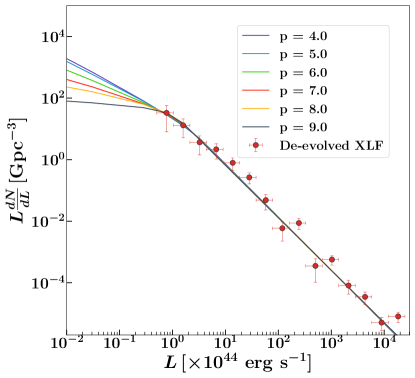
Figure 10: Best-fit to the de-evolved XLF ($\phi(L,0)$, red data points) using various values of the kinematic Doppler factor distribution index ($p$ parameter). Higher values of $p$ ($p>5$) are more likely attributed to EC process in the jet, while lower values are associated with the SSC process. As can be seen, for $p>7$ the XLF is predicted to show a break around the lowest luminosity bin of our sample ($L\sim 10^{44}\,\rm erg~{}s^{-1}$) while for lower values of $p$ this break would happen at $L<10^{42}\,\rm erg~{}s^{-1}$. From our best fits we are not able to discern which values are better representing the population of these jets, though the range $p=[5,7]$ seems to be the more favorable overall (see details in Section 7.1).

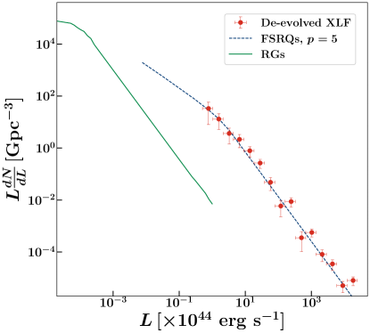
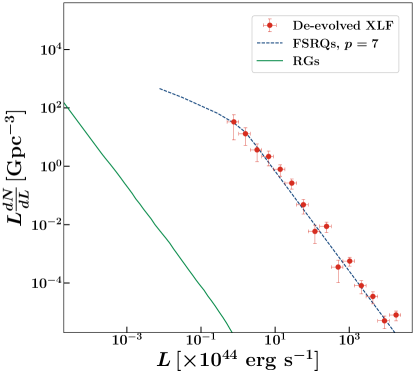
Figure 11: Results of the beaming fit to the BAT FSRQ population for $p=5$ (left) and $p=7$ (right). The red data points are the de-evolved luminosity function, $\phi(L,0)$, the blue dotted line is the fit derived for the FSRQ population, and the green line shows the distribution of the parent population (labeled here as RGs). As can be noted, different values of $p$ predict different number densities of the parent population at different luminosity bins. For $p=5$, RGs would show a break in the distribution at $L\sim 10^{41}\,\rm erg~{}s^{-1}$, luminosity at which they would be found with number densities of $10^{4}\,\rm Gpc^{-3}$. For $p=7$ instead this break would appear at even lower luminosities and their number densities at $L\sim 10^{41}\,\rm erg~{}s^{-1}$ would be two order of magnitudes lower with respect to $p=5$.

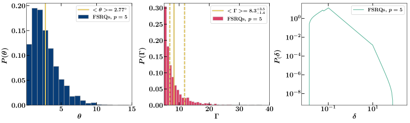
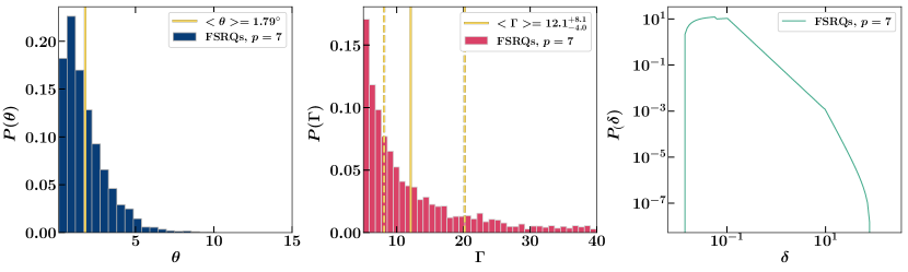
Figure 12: Distribution of $\theta$ ($P(\theta)$, normalized to 1), $\Gamma$ ($P(\Gamma)$, normalized to 1) and $\delta$ ($P(\delta)$) for the beaming fit to the BAT FSRQ population for $p=5$ (top) and $p=7$ (bottom). The average for the $\theta$ and $\Gamma$ distribution are shown by the yellow solid line. For the latter, the associated errors are represented by the yellow dashed lines. We note how a lower value of $p$ predicts lower average $\Gamma$, as well as a narrower range of predicted $\Gamma$ values, with respect to a higher value of $p$. On the other hand, the viewing angle distribution is broader for lower value of $p$, though they remain distributed between $1^{\circ}$ and $10^{\circ}$ and have an average $\theta\sim 2-3\degree$, quite independently of $p$.

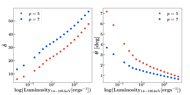
Figure 13: Median Doppler factors ($\widetilde{\delta}$, left) and median viewing angles ($\widetilde{\theta}$, right) as function of $14-195\,\rm keV$ luminosity derived from the beaming fit to the BAT FSRQ population for $p=5$ (red stars) and $p=7$ (blue dots). As the luminosity of the sources decreases, the $\delta$ factors become smaller and viewing angles get larger (corresponding to lower $\Gamma$ factors).

8 Discussion

In this work, we derive the most up-to-date BAT blazar luminosity function. We rely on a clean, significance limited, sample of 118 blazars (88 belonging to the FSRQ class) detected by the BAT at $>5\sigma$ above Galactic latitudes $|b|>10^{\circ}$ in 105 months of survey. An important thing to keep in mind for our work is that the FSRQ population dominates the inferences about our entire blazar sample. Being more numerous and detected to higher redshifts, these sources set the more stringent constraints for the derived luminosity function. BL Lac sources are mostly concentrated at low redshifts (only 2 sources have $z>0.36$), and 70% of them reside in the lowest luminosity bin of the derived XLF ($\log(L)=43.7-45.4\,\rm[erg~{}s^{-1}]$, see Table 1 and Figure 4). These objects have been found by previous work to show zero to mildly negative evolution (e.g., A14) and to contribute negligibly to the $14-195\,\rm keV$ background (see A09). In fact, looking at the consistent results between the evolution of FSRQs (Section 4.2) and the whole population (Section 4.1), we have deemed unnecessary to further investigate the BL Lacs evolution in the BAT energy range. It follows that, throughout this discussion, the word blazar is used as a synonym of FSRQ (and vice versa). Our main findings are listed and discussed below.

8.1 The blazar X-ray luminosity function

The blazar X-ray luminosity function derived in this work highlights several results. First, as discussed in Section 4, it is yet not possible to discern which kind of evolution takes place in this source class. Both density and luminosity evolution give compatible fits, of maximum likelihood values comparable to each other. This result is easily comprehended when plotting the luminosity function both in terms of redshift and luminosity (Figure 4). The lack of any significant break in the distribution is evident, which translates into the fact that PDE and PLE models are essentially indistinguishable from each other (Bahcall, 1977). This leads us to conclude that the BAT survey is still sampling only the high-luminosity blazar population at every redshift, while missing the bulk of the low-luminosity one. A slight hint of the occurrence of a break is present in the XLF model prediction for the lowest redshift bin (bottom plots of Figure 4). However, the statistical uncertainties related to its position remain large and its evolution with redshift and luminosity undetermined.

Another result is the fact that introducing a double power law to describe the local luminosity function, $\phi(L,V(z=0))$, significantly improves the fit. This feature is an expected consequence of the beaming effect and was already noticed by A09. The errors on the low-luminosity end slope are still quite large due to the lack of detection of many low-luminosity sources, but its value is compatible with the anticipated 1 to 1.5 from beaming predictions. Another expected and confirmed result is that the high-luminosity end of the BAT blazar distribution displays an index of $\gamma_{2}^{\prime}\sim 2.7$. In A09, this slope was found in the simple power-law luminosity function scenario but was not recovered in the double power-law case ($\gamma_{2^{\prime},\rm A09}\sim 3.7$), possibly due to the limited sample size. Therefore, our results using a larger and deeper sample confirm that the bright-end of the blazar luminosity function is consistent with the slope estimated for the unbeamed jetted AGN population (FRIIs luminosity function has been found to display a bright-end slope of $\gamma^{\prime}_{\rm FRII}\sim 2.65$, Cara & Lister, 2008, see).

In agreement with previous results, the derived evolutionary parameters, as well as the logN-logS trend, point to a positive evolution of the BAT blazar class (i.e., more/more luminous sources at earlier times). The values of $k$ are congruent between our work and A09, and they are consistently $>2$. For our best-fit mPLE, $k_{\rm mPLE}=3.23\pm 0.57$ (see Table 2) and in A09 $k_{\rm mPLE}=3.67\pm 0.48$. Moreover, we confirm that the peak of the high-luminosity BAT-FSRQ population is located at $z>4$. Differently than constrained only by upper limits in A09, our dataset extending up to $z=4.65$ allows us to measure the redshift peak directly. The peak position predicted by our best fit is $z_{\rm peak}=4.3\pm 1.0$, which is in good agreement with the $z_{\rm peak}=4.3\pm 0.5$ reported A09. Though our uncertainties on the position are larger than in A09, ML fits performed forcing the peak to be at a specific redshift confirm that it is more likely to occur between $z=4.3-4.4$ (see Section 4.2 for detailed description). Even at $z_{\rm peak}=4.6$ the fit results return maximum likelihood and parameter values consistent with our best-fit scenario (see Figure 6). This behaviour has strong implication in the number density of blazars expected at high redshift. As shown in Figure 5, number density values predicted at $z\sim 4$ are two times lower than those derived in A09.

This early evolutionary peak still remains very puzzling. In fact, LAT blazars (see Section 8.3), non-jetted AGN, galaxies, and star formation history of the universe are all found to coherently peak at $z\sim 2$. As pointed out in A09, the only other class of objects that resembles in evolution the most luminous BAT blazars is the massive elliptical galaxies one (De Lucia et al., 2006). Giant elliptical galaxies are understood to be a by-product of major merger events, which have also been shown to be a quick and viable mean to fast black hole accretion. In the chaotic high-redshift universe merger fractions have been found to be larger for highly massive galaxies even at $z>3$ (e.g., Bluck et al., 2009; Whitney et al., 2021). Therefore, one can picture a scenario in which there is a strong link between enhanced merging activity (leading to higher mass black holes and elliptical host galaxy morphology) and a jetted phase of the AGN in the early universe. The first evidence of a nascent jet possibly triggered by a merger was reported by Paliya et al. (2020b), further strengthening this scenario. Moreover the more luminous blazars are powered by the most massive black holes (see later), pointing to a further connection between jet activity and supermassive black hole growth. This envisaged paradigm also fits in the picture of cosmic “downsizing” of AGN activity, in which most massive and active black holes form quite early on, following the hierarchical build up of structures in the universe, and less powerful AGNs exist at later times (e.g., Trakhtenbrot & Netzer, 2012; Shen et al., 2020). Finally, as invoked in A09, if jets are powered through the Blandford & Znajek (1977) mechanism, then they may be tapping into an extra reservoir of energy provided by the black hole spin. Positive evidence that jets are indeed more powerful than their accretion disks has been found even for sources at $z>3$ (e.g., Ghisellini et al., 2014; Paliya et al., 2017). Calculations for major merger events also show how these can produce maximally spinning black holes (see Berti & Volonteri, 2008; Volonteri, 2010) and that high-redshift black holes spin faster than their lower redshift counterpart (e.g., Volonteri et al., 2016). Therefore not only these powerful blazars help us trace the evolution of massive black holes in the early universe, but also the history of black hole spins.

8.2 Number Density of Blazars and Parent Population

The Doppler boosting affecting the jet emission allows us to derive the properties of the parent population of randomly oriented jets (Section 7). A few caveats have to be taken into consideration while examining these results. Firstly, an expected outcome of beaming on the local luminosity function is a flattening of the low-end of $\phi(L,V(z=0))$, which is not yet clearly seen in our sample. Therefore, the fit parameters have large uncertainties. Secondly, the possible explored values of $p$ (the index of the kinematic Doppler factor distribution) strongly relies on the jet configuration as well as emission processes. The finding that the high-energy SED peak location does not strongly depend on the source luminosity (Section 5), is suggestive of the fact that EC process is dominant in the considered sample. Therefore, higher values of $p$ (e.g., $p=5-7$) should be considered as more relevant for the population.

The fit enables us to derive the power-law distribution bulk Lorentz factors, which is shown in its normalized version in the middle panels of Figure 12 for two values of $p$. Our result show that higher values of $p$ predict a distribution of jets with on average higher bulk Lorentz factors and has a larger spread (between the chosen $\Gamma=[5,40]$). If we compare with the results of A12 on LAT blazars, for $p=5$ the $\Gamma$ distribution is less steep ($\mu_{\rm LAT}=-2.43\pm 0.11$ vs. $\mu_{\rm BAT}=-3.33\pm 1.30$ ) and the average $\Gamma$ is higher ($<\Gamma_{\rm LAT}>=10.2_{-2.4}^{+4.8}$ vs. $<\Gamma_{\rm BAT}>=8.3_{-1.4}^{+3.5}$). This is in very good agreement with the outcome from radio monitoring of LAT blazars by the VLBA (e.g., Lister et al., 2009), which shows that LAT detected blazar jets have, on average, higher velocities that non-LAT detected ones. It is interesting to notice that recent single source studies on high-redshift blazars with combined hard X-ray and $\gamma$-ray detection (e.g., Ajello et al., 2016; Marcotulli et al., 2017; Ackermann et al., 2017; Marcotulli et al., 2020b) find that the jet powers could be lower than previously thought for these sources (i.e., average $\Gamma\sim 9-10$, instead of the canonical $15$, Sbarrato et al., 2015). Lower values of $\Gamma$ for these high-redshift luminous blazars (cf. Paliya et al., 2020a) have strong implication on supermassive black holes space densities (Section 8.4).

The distribution of jet viewing angles derived through the fit is very narrow (left panels of Figure 12). This can be understood in view of the fact that the most luminous and highest redshift sources have to be extremely aligned (and have high $\Gamma$ factors) for them to be detected in the BAT band. On the other hand, the lower luminosity sources, residing at lower redshifts (see Figure 2) can be found a larger viewing angles ($\theta_{\rm max}\sim 10\degree$) and with lower $\Gamma$ factors. The distributions of $\delta$ factors and viewing angles as function of BAT luminosity (Figure 13) highlight these strong geometrical selection effects, which are also visible in the $14\,\rm keV$ to $10\,\rm GeV$ average SED of these sources (see right panel of Figure 7 and Section 5.2). As the source luminosity decreases, the peak position slightly shifts towards lower energies ($\Delta E_{b,\rm rest-frame}\sim 10\,\rm MeV$), indicative of lower $\delta$ of the jets (e.g. Ghisellini, 2015; Sbarrato et al., 2015; Lister et al., 2019; Paliya et al., 2019). Finally, the shape derived for the intrinsic luminosity function ($B=2.73\pm 0.05$) is in agreement the spectral slope of the blazar XLF ($\gamma_{2}^{\prime}\sim 2.7$) as well as the one of the unbeamed jetted AGN.

Number densities of the parent population are strongly affected by the value of $p$, and can change by orders of magnitude depending on the resulting fit (see Figure 11). The derived percentage of FSRQs to the total number density of their parent population is $\sim 0.1\%$ for the case $p=5$ (i.e., one jet out of a hundred would be detected in the blazar orientation), while higher values of $p$ make these estimate decrease by order of magnitudes (i.e. for $p=7$, one jet in a thousand would be detected as blazar). Considering the derived number densities of blazars and the distribution of $\Gamma$, we could estimate the number densities of parent population applying the $2\Gamma^{2}$ correction as well as its modified formulation from Lister et al. (2019). The results are quite similar in values with the two approaches, implying the existence from a few to more than 10 thousands jets in the universe (depending on the chosen luminosity bin, see Table 4). The low-mid luminosity estimates are consistent with the estimated number density of FRII (Cara & Lister, 2008), which is $\sim 1.6\times 10^{3}\,\rm Gpc^{-3}$ (for $L_{\rm 15GHz}\geq 1.3\times 10^{25}\,\rm W~{}Hz^{-1}$), though the total number of parents is higher than the one so far predicted for FRIIs. Overall, values of the $p$ parameter in the range $5-7$ provide a better description of our jet distribution.

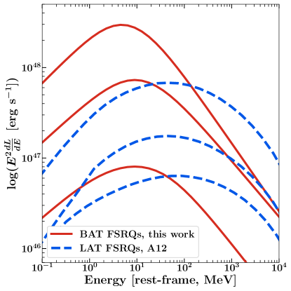
Figure 14: Comparison between average BAT-blazar and LAT-blazar SEDs. BAT blazar SEDs are shown by the magenta solid lines and are the ones derived from this work in the X-ray luminosity bins ($\log L_{\rm BAT}=[46.6,47.3],[47.3,48.3],[48.3,48.8]\,\rm erg~{}s^{-1}$, see also Figure 7). The LAT SEDs are the ones reported in A12 for the bolometric luminosity (derived in their work from the $\gamma$-ray luminosity) bins $\log L_{\rm bol}=[47.6,47.9],[47.9,48.5],[48.5,49.3]\,\rm erg~{}s^{-1}$ and are shown by the blue dashed lines. This Figure highlights that BAT blazars have their high-energy peak located at lower energies than the LAT sources. Moreover, both classes of objects do not show strong evolution of the SED shape and/or peak depending on the chosen luminosity bin.

8.3 MeV versus GeV blazars

Hard X-ray and $\gamma$-ray blazars have been surmised to belong to the same source population, but carrying slightly different characteristics. The most luminous FSRQs detected by BAT belong to the class referred to as ‘MeV blazars’. Their high-energy SED, as derived in Section 5, peaks in the MeV band ($E_{b,\rm rest}\sim 3-17\,\rm MeV$), and they are extremely luminous, capable of reaching $L_{\rm bol}>10^{49}\,\rm erg~{}s^{-1}$. Single source studies of these MeV blazars usually find that their high-energy emission is dominated by the EC process rather than SSC. Further evidence confirming this scenario lies in our derived average $14\,\rm KeV-10\,\rm GeV$ SED (Section 5 and Figure 7), which shows similar slopes as well as peak positions, independently of the luminosity bin considered. This behaviour is in contrast with the anti-correlation found instead for the low-energy synchrotron peak component (e.g., Padovani et al., 1998; Ghisellini et al., 2017) and in the high-energy SED of high-synchrotron peaked BL Lacs (which instead agree with the SSC paradigm). The lack of strong luminosity dependence on the peak position of the SED makes the jet parameters independent on X-ray luminosity or redshift. In turn, this translates into the fact that the BAT FSRQs belong to a population with homogeneous properties. In Figure 14 we overlay our average BAT-blazar SED and the LAT-blazar SED from A12. As can be seen, the high-energy SED of LAT FSRQs shows a peak between $E_{b,\rm rest-frame}\sim 50-100\,\rm MeV$, and they are on average less luminous than the BAT ones. Their emission, similarly to BAT FSRQs, is attributed to EC emission from the jet and their spectral shape does not show a strong evolution as function of luminosity. Interestingly, the shape of the XLF at $z=0$ is very similar to the $\gamma$-ray luminosity function (GLF) in terms of spectral indices (while the normalization and typical break luminosity differs).

Slight differences between the two classes appear in the derived jet properties of the parent population. The BAT-blazar jets are found to be on average slower than the LAT detected ones (for $p=5$, $\Gamma_{\rm BAT}=8.3$ vs. $\Gamma_{\rm LAT}=10.2$). Predicted number densities for LAT FSRQs are $\sim 1500\,\rm Gpc^{-3}$ while for BAT FSRQs these may be as high as $10^{4}\,\rm Gpc^{-3}$. Major differences between the two classes are (1) their typical average luminosities, and (2) their evolutionary properties. In fact, in terms of evolution, it had been surmised that since the high-energy emission is ascribed to the same radiative process for both classes, then their evolution should be similar, if not the same. However, discrepancies have been noticed. LAT FSRQs have a peak in the evolution at $z_{\rm peak}\sim 1.6$ after which their space density decreases quickly. This peak occurs significantly later than the one derived here for the most luminous BAT FSRQs ($z_{\rm peak}\sim 4.3$). Recent works have also highlighted that a PDE evolution may be taking place in the LAT blazar sample (Marcotulli et al., 2020a) while in this work we find that a luminosity evolution seems to be favored. Furthermore, BAT FSRQs are powered on average by more massive black holes than the LAT FSRQs (see, Ghisellini et al., 2017; Paliya et al., 2019, 2021).

These properties suggest that hard X-ray and $\gamma$-ray blazars belong to the same family of sources, with the same homogeneous properties, which has undergone a two-phase evolutionary sequence. In line with the discussion in Section 8.1, this could mean that these jets and their black holes are following the cosmic downsizing: the most extreme and luminous jets powered by the most massive black holes (BAT blazars) peak earlier in cosmic history, to then become less powerful in the late universe (LAT blazars), tracing more closely the evolution of the non jetted AGNs (e.g., A12, Ueda et al., 2014; Aird et al., 2015; Shen et al., 2020).

Differences in evolutionary paths of BAT and LAT blazars have been already reported in previous works (A09, A12, A14, Toda et al., 2020), and possibly a combined LAT-BAT-detected blazar luminosity function study is due. Alternatively, an all-sky MeV instrument (e.g., COSI, Tomsick et al., 2019; AMEGO-X, Caputo et al., 2022, see Section 8.5) would enable us to produce new measurements of the background in the MeV energy range, to pinpoint the peak of the SED of these powerful blazars, and to understand what type of evolutionary scenario is taking place in this source class.

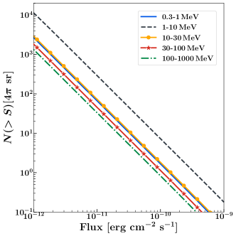
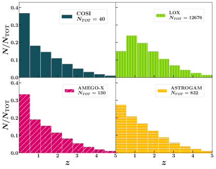
Figure 15: Left: predicted logN-logS from our best-fit XLF and SED models in different MeV bands. It can be seen that an instrument with a uniform sensitivity of $S=10^{-12}\,\rm erg~{}cm^{-2}~{}s^{-1}$ would be able to detect between $10^{3}$ and $10^{5}$ sources (depending on the energy range). Right: histogram of fraction of sources as function of redshift expected to be detected by proposed MeV mission (see Section 8.5).

8.4 Supermassive black hole space density

The work of Sbarrato et al. (2015) showed how for radio-loud (i.e., jetted) quasars the supermassive black hole (SMBH, $M_{\rm BH}>10^{9}M_{\odot}$) space density peaks earlier than radio-quiet (i.e., no jets) AGNs. The authors considered the evolution of BAT blazars derived by A09 and employed the $2\Gamma^{2}$ correction to infer these densities. However, two key assumptions had taken place: first that all $L>10^{47}\,\rm ergs^{-1}$ host $M_{\rm BH}>10^{9}M_{\odot}$, and second that the average $\Gamma$ factor is $\sim 15$.

Firm spectroscopic mass measurements are confirming that the most powerful blazars indeed host black holes with $M_{\rm BH}>10^{9}M_{\odot}$. On the other hand, in our work we find that on average the value of $\Gamma$ factors derived for these jets could be lower than previously assumed. This has implication on SMBHs space densities of jetted sources. In fact, the authors derive the number density of SMBH traced by radio-loud sources to be $\sim 60\,\rm Gpc^{-3}$ at $z_{\rm peak}\sim 4$. A Lorentz factor such as $6-8$ could lower this estimate by almost an order of magnitude. Finally, we note that according to our derived evolutionary function, the number density of luminous jets is lower at $z>4$ than previously derived, and recall that the $2\Gamma^{2}$ may be an incorrect approximation when assessing the size of the parent population. Possibly a combination of better constrained LF and derived jet properties can help up shed a light on the population of supermassive black holes in the early universe. This conundrum could also be helped by a deeper X-ray survey combined with multi-wavelength single source studies.

8.5 Prospects for the MeV range

The contribution of blazars to the CXB background, according to our best fit model, can range between $5-20\%$ in the $14-195\,\rm keV$ band. Therefore they are subdominant in this energy range. It is worth nothing that these limits will not significantly improve with longer BAT surveys, owing to the fact that the significance gain goes as $\sqrt{t}$ ($t$ being the time covered by the survey). On the other hand, this source population has been found to contribute $>50\%$ of the EGB (depending on the energy range even up to $100\%$, see e.g. Ackermann et al., 2015; Di Mauro et al., 2018; Marcotulli et al., 2020a). The most powerful of these jets have also been surmised to account for most of the MeV background. Indeed, as derived in Section 5, the average SED of FSRQs peaks at $\sim 3-17\,\rm MeV$, i.e., the most of their energy output falls in the MeV band.

In this work, we have extrapolated the contribution of powerful BAT FSQRs to the MeV background. From Figure 9, it can be seen how indeed the MeV background could be entirely produced by blazars alone. It is known that other source populations could contribute as well, up to few %, to the MeV background. Our best-fit mPLE model convolved with the average SED does have large uncertainties in the MeV band, hence allowing for contribution from other source classes. Only an MeV mission would provide the opportunity to constrain the background level and shape to a higher significance (latest reported by COMPTEL, Weidenspointner et al., 2000), as well as unveil the bulk of these blazar sources.

With the best fit XLF and the blazar SED in hand, we can make prediction on the expected logN-logS from these powerful BAT FSRQs in the MeV band. The cumulative source count distribution, $N(>S)$, is given by Equation 14. To extrapolate this function to a different energy range, it is necessary to allow the lower limit of the integral to become energy dependent, $L_{\rm min}(S_{\rm E_{1},E_{2}},z)$. Therefore, the luminosity relies on the SED shape, and $S_{\rm E_{1},E_{2}}$ is the flux limit in the requested energy range. It follows that the lower limit in luminosity depends on the flux sensitivity of the mission, at specific energy ranges. For the purpose of this derivation, however, we consider an arbitrary minimum flux of $10^{-13}\,\rm erg~{}cm^{-2}~{}s^{-1}$. The results are shown in the left panel of Figure 15 (right panel) for the energy bins $[0.3,1,10,30,100,1000]\,\rm MeV$, similarly to the ones chosen by Inoue et al. (2015). It can be seen how the number of blazars detectable by an instrument with sensitivity $S>10^{-12}\,\rm erg~{}cm^{-2}~{}s^{-1}$ will be of the order of $10^{3}$ to $\sim\times 10^{4}$.

Table 5: Prediction of total number of sources per $4\pi$ sterad and number of sources as a function of redshift for future MeV mission (and eROSITA).

	Band	Sensitivity	Total	$0\leq z<1$	$1\leq z<2$	$2\leq z<3$	$3\leq z<4$	$4\leq z<5$
		$[\rm erg~{}cm^{-2}~{}s^{-1}]$	$0\leq z<5$
COSI	$0.2-5\,\rm MeV$	$S>4\times 10^{-11}$ (2 yrs, Tomsick et al., 2019)a	40	20	10	6	3	1
AMEGO-X	$1-10\,\rm MeV$	$S>1.6\times 10^{-11}$ (3 yrs, Caputo et al., 2022)	130	63	34	20	9	4
ASTROGAM	$1-10\,\rm MeV$	$S>5\times 10^{-12}$ (1 yr)b	832	367	241	137	63	24
LOX	$0.1-3\,\rm MeV$	$S>10^{-12}$ (1 yr, Miller et al., 2019)	12676	4279	4339	2472	1135	451
eROSITA	$0.2-2\,\rm keV$	$S>10^{-14}$ (1 yr, Predehl et al., 2021)	230023	23681	86786	70403	34981	14172

Finally, with the obtained XLF we can make predictions on how many sources per redshift bin would be detectable by an MeV experiment with a certain sensitivity. We consider estimated sensitivities of proposed and accepted MeV missions: COSI (point source sensitivities obtained via private communication, see Tomsick et al., 2019); AMEGO-X (Caputo et al., 2022); ASTROGAM (point source sensitivities reported in the mission design proposed for the M7 mission call of ESA, obtained via private communication); LOX (Miller et al., 2019). Table LABEL:tab:mev_pred reports the predicted sensitivities and number of sources that will be detected by such missions in various redshift bins, and the normalized histogram showing the fraction of sources detected per redshift bin by these missions is shown in the right panel of Figure 15. For comparison we also list the prediction for eROSITA (Predehl et al., 2021). If we use the mPLE evolution model, it can be seen how we expect that tens of blazars would be detected even beyond $z>4$, and several up to a $z\sim 5-6$. Recently, Wolf et al. (2021) has pointed out how the XLF of QSOs may predict more sources than expected at higher redshifts. In particular, the source they studied with eROSITA data is located at $z=5.81$ and may harbor a nascent jet. This could be a progenitor to radio-loud quasars considered in this work, and might imply the existence of many such powerful sources earlier than $z>4$. Some of these high-$z$ blazars, or nascent jets may have already been detected at $z>4$ (see Zhu et al., 2019). Only an instrument with a deeper sensitivity either in hard X-rays or in the MeV band could unveil the bulk of these high-$z$ powerful jets.

8.6 Neutrino Predictions

Blazars in general, and MeV blazars in particular, are thought to be possible sources of extragalactic neutrinos (e.g., Murase et al., 2014, 2016; Kadler et al., 2016; Aartsen et al., 2017; Krauß et al., 2018; IceCube Collaboration et al., 2018; Buson et al., 2022). Taking advantage of the derived best-fit high-energy SED and of the up-to-date XLF, we calculate the number of neutrinos expected to be found in coincidence with MeV blazars detected by a forthcoming MeV mission (de Angelis et al., 2018; Tomsick et al., 2019; Miller et al., 2019; Caputo et al., 2022). We follow the methodology described in Krauß et al. (2018, and references therein), whose main assumptions are: (i) the integrated neutrino flux between $30\,\rm TeV$ and $10\,\rm PeV$ is equivalent to the high-energy flux emitted by MeV blazars integrated between $0.1\,\rm keV$ and $1\,\rm TeV$ ($\phi_{\nu}=\phi_{\gamma}$, see also Krauß et al., 2014); (ii) the neutrino spectrum follows a power law ($dN_{\nu}/dE_{\nu}\propto E^{-\Gamma_{\nu}}$) of index $\Gamma_{\nu}=2.58$ (The IceCube Collaboration et al., 2015). The total number of neutrinos expected from one single MeV blazar is therefore:

$$\begin{split}N_{\nu}=\sum_{i=0}^{N-1}&\int^{E^{\prime}_{i+1}}_{E^{\prime}_{i}}\frac{dN_{\nu}}{dE_{\nu}}dE_{\nu}=\\ =&\frac{\phi_{\gamma}(2-\Gamma_{\nu})}{E_{2,\nu}^{2-\Gamma_{\nu}}-E_{1,\nu}^{2-\Gamma_{\nu}}(1-\Gamma_{\nu})}T_{\rm eff}\times\\ \times&\sum_{i=0}^{N}A_{\rm eff}(E_{\nu}^{\prime})(E_{i+1}^{\prime 1-\Gamma_{\nu}}-E_{i}^{\prime 1-\Gamma_{\nu}}).\\ \end{split}$$ (27)

In the above, $A_{\rm eff}$ is the IceCube effective area evaluated in the energy bin $[E^{\prime}_{i},E^{\prime}_{i+1}]$; $E_{\nu}$ is the mean energy of the $i^{th}$ bin; the sum runs from $E^{\prime}_{0}=E_{1,\nu}=30\rm\,TeV$ to $E^{\prime}_{N}=E_{2,\nu}=10\rm\,PeV$; $\phi_{\gamma}$ is calculated from the best-fit SED of Section 5.2. For simplicity, we take the available IceCube neutrino effective area from Krauß et al. (2018, Figure 1) calculated using 4 years of data ($T_{\rm eff}=1347$ days). Furthermore, to obtain a more realistic number of detectable neutrinos, $N_{\nu}$ has to be corrected by: (1) an empirical factor ($f=0.009$, Kadler et al., 2016) that takes into account physically motivated blazar spectra; (2) the ratio between the 4 yr IceCube exposure and the exposure of the considered MeV instrument ($t=T_{\rm MeV}/T_{\rm eff}$). This reduces the expected number of neutrinos from one source to:

$$N_{\nu,det}=N_{\nu}\times ft.$$ (28)

Considering an MeV mission, with its sensitivity limit ($S_{\rm lim}$) over a certain time period ($T_{\rm MeV}$) in a specific energy band, it is possible to estimate the expected number of detectable sources and their flux distribution (see Section 8.5). For every detectable source, we randomly extract its MeV flux from the relevant logN-logS and calculate $N_{\nu,det}$. Importantly, we estimate the number of coincident detections as the number of blazars that are able to produce at least one neutrino, which could be detected by IceCube, within the observing window of the MeV mission ($T_{\rm MeV}$).

Table 6: Predictions on number of coincidence detections of neutrinos from MeV blazars by IceCube, considering future MeV missions (Section 8.6).

	Number of Coincident Detectionsa
COSI	$2^{+1}_{-1}$
AMEGO-X	$4^{+1}_{-1}$
ASTROGAM	$5_{-1}^{+1}$
LOX	$11_{-2}^{+1}$

We perform this calculation 10000 times and extract the median number of coincident detections for all MeV missions listed in Table 5. The results are reported in Table 6. The median number of coincident detections ranges from $2-12$. This implies that, for example, COSI will detect (in its 2 year survey) 2${}^{+1}_{-1}$ blazars with coincident detection by IceCube. We note that these numbers are quite conservative as we do not take into account the possibility of flares. Blazars are known to be extremely variable at all wavelengths, and in particular at $\gamma$-ray energies where the emission is dominated by the higher energy particles (e.g., Abdo et al., 2010; IceCube Collaboration et al., 2018; Nesci et al., 2021; Malik et al., 2022). A significant increase in neutrino flux is therefore expected when the sources are detected in their flaring state (see e.g., Murase et al., 2018). Indeed, even a factor of 5 flux increase would imply a number of coincident detections of $9_{-2}^{+1}$ in the COSI $2\,\rm yrs$ survey. Finally, a longer exposure time when IceCube and an MeV mission are both operative would ensure a larger number of coincident detections.

9 Summary & Conclusions

In this work we have derived the most up-to-date BAT blazar X-ray luminosity function in the $14-195\rm\,keV$ range. The main results are summarized as follows:

1. BAT blazars evolve positively in redshift, indicating the presence of more (or more luminous) sources at earlier cosmic times. The peak in space density of this population is located at $z_{\rm peak}\simeq 4.3\pm 1.0$. In terms of number densities, these sources are predicted to be less numerous at higher redshifts compared with previous works.

2. The blazar XLF at every redshift bin is distributed (in $\log-\log$ space) according to a straight power law of index $\gamma_{2}=1.67\pm 0.19$. Lack of any spectral break in the XLF impedes us to confirm whether the evolution of these source class happens in luminosity or density. Nonetheless, fit results confirm with high significance that a break in the local XLF at the level of the last observed luminosity ($L_{\rm min}=10^{44}\,\rm erg~{}s^{-1}$) is favored, and the index of the low-luminosity end flattens as expected from beaming.

3. We derive the average SED of BAT FSRQs (with and without LAT detection) in the range $14\,\rm keV$-$10\,\rm GeV$ in order to understand their contribution to the cosmic high-energy background. In the $14-195\,\rm keV$ blazars can contribute at most $\sim 20\%$. On the other hand, these powerful sources are found to be able to potentially contribute $\sim 70-100\%$ of the MeV background in the $0.5-30\,\rm MeV$ range (depending on the evolutionary model). Predictions from the density evolution model are shown to slightly overestimate the MeV background level, implying that a luminosity evolution is more likely favored by these sources as it allows for contribution from other known MeV emitting sources.

4. Properties of the jets parent population are derived in this work. The intrinsic luminosity function is confirmed to be distributed similarly to the unbeamed jetted AGNs ($B=2.7$). For the selected blazar sample, the average viewing angles are very narrow ($\theta=2-3\degree$) and the average speeds of the jet plasma is lower than previously expected ($<\Gamma>=8-12$). This has implication on the power of these sources, which could be lower than previously assumed, as well as on their number densities which could decrease up to an order of magnitude (considering the $2\Gamma^{2}$ correction, see Section 8.4).

5. BAT blazars (mostly comprising FSRQ-type sources) are found to be more luminous than LAT detected sources and host more massive black holes. Lack of strong evolution in the SED and XLF properties suggest that these two source classes belong to the same parent population. The difference in evolution (i.e., BAT blazar peak at earlier cosmic times and most likely follow a luminosity evolution while LAT blazars likely undergo a density evolution and peak at $z\sim 2$) indicate that blazars may be following the paradigm of AGN cosmic downsizing.

6. Finally, prediction for number counts of sources in the MeV range are derived, implying detection on the order of hundreds or thousands of sources up to redshift $5-6$, making the prospects for MeV blazar science very promising in light of an upcoming MeV mission. Furthermore, the estimated number of high-energy neutrino detection by IceCube in coincidence with MeV blazars within the observing window of forthcoming MeV missions is derived. The expectation is that IceCube should detect 2 coincident neutrinos in a 2 year MeV survey like COSI.

Appendix A Source Count Distribution

In order to assess whether the discrepancy between the derived logN-logS and the model predictions (seen in Figure 3) at fluxes $F_{\rm 14-195\,keV}<8\times 10^{-12}\,\rm erg~{}cm^{-2}~{}s^{-1}$ affects our results, we perform an XLF fit to the total blazar sample removing sources with $F_{\rm 14-195\,keV}<8\times 10^{-12}\,\rm erg~{}cm^{-2}~{}s^{-1}$ (12/118 sources, 3 of which have $z>1$). For consistency, we also use the efficiency above this threshold flux. We employ the same maximum-likelihood fitting technique described in Section 3.1 and test both the mPDE and mPLE parametrizations. The obtained fits show that both the mPDE and the mPLE results are consistent with the ones derived for the whole sample (cfr. Table 2 and Table 7).

The differential logN-logS for the total 118 beamed AGN sample is also shown in Figure 16. As can be seen, within the statistical uncertainties the best-fit model predictions are consistent with the data. This allows us to conclude that the full sample of 118 sources is representative of the BAT-blazar population and that possible discrepancies at low fluxes (possibly arising from sky coverage calculations or sources missed as blazars at low fluxes) do not influence our results.

Table 7: Result of the maximum likelihood fit only including sources $F_{\rm 14-195\,keV}>8\times 10^{-12}\,\rm erg~{}cm^{-2}~{}s^{-1}$ (see Appendix A).

SAMPLE	LF	Parameters						$C$	CXB
Total		Aa	$L_{*}^{b}$	$\gamma_{1}$	$\gamma_{2}$	k	$\xi$
	mPLE	$1.70\pm 0.16$	$1.60\pm 1.05$	$-0.38\pm 1.19$	$2.03\pm 0.23$	$3.59\pm 0.53$	$-1.57\pm 0.40$	1308.42	10.23%
		Aa	$L_{*}^{b}$	$\gamma_{1}$	$\gamma_{2}$	k	$\xi$
	mPDE	$1.59\pm 0.15$	$1.54\pm 0.84$	$-0.65\pm 1.32$	$1.97\pm 0.20$	$10.52\pm 2.23$	$-0.53\pm 0.16$	1308.62	115.14%

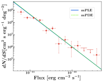
Figure 16: Differential BAT-blazars logN-logS, i.e., number of sources per flux bin corrected for the survey sky coverage, $dN/dS$, as a function flux. The observed differential logN-logS is represented by the red data points, while the blue solid and green dashed lines show the prediction from the best-fit mPLE and mPDE models, respectively. The error bars are calculated using Poisson statistics.

Table 8: Table of clean sample used in the analysis.

No.a	Nameb	RAc	DECc	Assoc. Ctpt.d	$\sigma^{e}$	Typef	$F_{\rm 14-195\rm keV}^{g}$	$\Gamma_{\rm 14-195\rm keV}^{h}$	$z^{i}$
	[SWIFT]	$[\rm^{\circ},J2000]$	$[\rm^{\circ},J2000]$				$[10^{-12}\,\rm~{}erg~{}cm^{-2}~{}s^{-1}]$
8	J0010.5+1057	2.61	10.96	Mrk 1501	14.02	BZQ	$30.34_{-2.80}^{+3.06}$	$1.82\pm 0.21$	0.089
9	J0017.1+8134	4.48	81.56	[HB89] 0014+813	8.57	BZQ	$11.39_{-1.86}^{+2.08}$	$2.42_{-0.43}^{+0.53}$	3.366
30	J0042.9+3016B	10.70	30.28	2MASX J00423991+3017515	11.4	BZQ	$26.08_{-9.51}^{+12.67}$	$0.5_{-...}^{+1.36}$	0.140
48	J0103.8-6437	15.94	-64.63	PKS 0101-649	7.19	BZQ	$14.3_{-1.48}^{+2.48}$	$1.58_{-0.51}^{+0.54}$	0.163
59	J0113.8+2515	18.41	25.29	WISE J011322.69+251853.2	5.52	BZQ	$8.70_{-2.43}^{+2.98}$	$2.09_{-0.72}^{+0.93}$	1.589
71	J0122.9+3420	20.77	34.37	SHBL J012308.7+342049	9.23	BZB	$11.27_{-1.62}^{+2.06}$	$2.94_{-0.48}^{+0.61}$	0.272
1228	J0131.5-1007	22.88	-10.13	SDSS J013126.71-100931.1	6.48	BZQ	$12.84_{-2.84}^{+3.04}$	$1.81_{-0.48}^{+0.53}$	3.515
1235	J0156.5-5303	29.13	-53.03	RBS 259	5.49	BZB	$7.32_{-2.46}^{+1.56}$	$2.31_{-0.51}^{+0.60}$	0.3043
1237	J0201.0+0329	30.29	3.57	[HB89] 0158+031	6.93	BZQ	$10.71_{-2.87}^{+2.46}$	$2.25_{-0.65}^{+0.99}$	1.581
120	J0218.0+7348	34.38	73.80	[HB89] 0212+735	15.5	BZQ	$34.98_{-2.43}^{+2.31}$	$1.55\pm 0.18$	2.367
125	J0225.0+1847	36.25	18.80	RBS 0315	14.15	BZQ	$31.37_{-2.91}^{+3.47}$	$1.73\pm 0.22$	2.690
132	J0232.8+2020	38.18	20.28	QSO B0229+200	13.85	BZG	$23.46_{-2.27}^{+2.62}$	$2.28_{-0.28}^{+0.31}$	0.139
1243	J0233.8+0243	38.43	2.43	IGR J02341+0228	5.13	BZQ	$7.02_{-1.26}^{+2.72}$	$2.69_{-0.71}^{+1.08}$	0.321
1244	J0244.8-5829	41.18	-58.29	BZB J0244-5819	8.39	BZB	$10.13_{-1.13}^{+2.46}$	$2.43_{-0.42}^{+0.52}$	0.264
148	J0245.2+1047	41.32	10.77	4C+10.08	8.05	BZG	$18.3_{-2.44}^{+2.71}$	$1.70_{-0.43}^{+0.48}$	0.070
1246	J0250.8-3626	42.69	-36.26	6dF J0250552-361636	5.23	BZQ	$10.01_{-1.53}^{+3.36}$	$1.73_{-0.60}^{+0.03}$	1.536
1254	J0304.6+3348	46.18	33.80	4C +33.06	5.25	BZQ	$11.89_{-3.29}^{+2.51}$	$1.86_{-0.51}^{+0.57}$	0.681
1257	J0310.7+3917	47.74	39.23	WISE J031024.53+391057.9	6.1	BZQ	$9.90_{-3.19}^{+2.42}$	$1.89_{-0.55}^{+0.66}$	0.370
168	J0311.8-7653	47.75	-76.86	[HB89] 0312-770	6.89	BZQ	$10.47_{-2.06}^{+2.24}$	$1.98_{-0.48}^{+0.57}$	0.223
178	J0326.0-5633	51.47	-56.52	2MASX J03252346-5635443	6.62	BZG	$8.49_{-2.21}^{+2.35}$	$2.06_{-0.54}^{+0.66}$	0.060
188	J0336.6+3217	54.12	32.29	4C+32.14	16.9	BZQ	$44.17_{-3.05}^{+3.16}$	$1.67_{-0.17}^{+0.16}$	1.258
192	J0349.2-1159	57.36	-11.98	QSO B0347-121	9.75	BZG	$15.68_{-2.25}^{+3.31}$	$2.20_{-0.36}^{+0.42}$	0.187
195	J0353.4-6830	58.28	-68.53	PKS 0352-686	10.03	BZB	$12.24_{-1.44}^{+1.67}$	$2.52_{-0.36}^{+0.43}$	0.087
206	J0404.0-3604	60.96	-36.07	PKS 0402-362	6.6	BZQ	$10.65_{-1.87}^{+2.48}$	$1.91_{-0.50}^{+0.61}$	1.417
208	J0405.5-1307	61.35	-13.14	[HB89] 0403-132	5.75	BZQ	$11.03_{-3.44}^{+2.37}$	$1.78_{-0.59}^{+0.69}$	0.570
1271	J0407.9-1219	61.98	-12.19	[HB89] 0405-123	5.89	BZQ	$8.14_{-2.34}^{+1.89}$	$2.56_{-0.60}^{+0.79}$	0.572
210	J0413.3+1659	63.34	16.96	MG1 J041325+1659	6.51	BZQ	$15.17_{-4.00}^{+2.77}$	$1.88_{-0.51}^{+0.60}$	0.212
1278	J0506.6-1937	76.69	-19.62	2MASX J05064796-1936507	5.03	BZQ	$13.56_{-3.38}^{+3.16}$	$1.31_{-0.55}^{+0.56}$	0.094
259	J0507.7+6732	76.91	67.53	87GB 050246.4+673341	6.7	BZB	$9.03_{-2.28}^{+2.18}$	$2.50_{-0.57}^{+0.81}$	0.314
276	J0525.1-2339	81.27	-23.66	PMN J0525-2338	5.78	BZQ	$13.11_{-3.59}^{+2.80}$	$1.55_{-0.51}^{+0.55}$	3.100
1282	J0538.5-4411	84.63	-44.11	[HB89] 0537-441	5.12	BZB	$14.86_{-2.77}^{+2.58}$	$0.88_{-...}^{+0.69}$	0.894
296	J0539.9-2839	84.96	-28.69	[HB89] 0537-286	11.67	BZQ	$29.01_{-3.50}^{+2.67}$	$1.33\pm 0.26$	3.104
306	J0550.7-3212A	87.68	-32.27	PKS 0548-322	26.92	BZB	$18.21_{-5.29}^{+6.16}$	$3.23_{-1.23}^{+2.34}$	0.069
1289	J0608.9-5507	92.20	-55.07	PKS 0607-549	5.14	BZQ	$6.24_{-3.72}^{+3.68}$	$2.19_{-...}^{+5.84}$	2.460
323	J0612.2-4645	93.06	-46.74	PMN J0612-4647	5.82	BZQ	$6.85_{-1.41}^{+1.78}$	$2.47_{-0.62}^{+0.88}$	0.317
327	J0623.3-6438	95.85	-64.61	2MASX J06230765-6436211	7.31	BZQ	$11.64_{-1.62}^{+2.09}$	$1.98_{-0.45}^{+0.53}$	0.128
340	J0635.8-7514	99.01	-75.27	PKS 0637-752	9.57	BZQ	$16.52_{-1.83}^{+2.78}$	$2.00_{-0.30}^{+0.35}$	0.651
361	J0710.3+5908	107.63	59.14	2MASX J07103005+5908202	15.38	BZB	$24.06_{-2.29}^{+2.77}$	$2.28_{-0.24}^{+0.26}$	0.125
1308	J0721.0+7133	110.49	71.33	[HB89] 0716+714	6.39	BZB	$19.04_{-2.48}^{+2.68}$	$1.15_{-0.43}^{+0.39}$	0.300
377	J0733.9+5156	113.40	51.93	2MASX J07332681+5153560	5.38	BZG	$8.17_{-2.17}^{+2.27}$	$2.32_{-0.71}^{+0.93}$	0.065
387	J0746.3+2548	116.58	25.80	B20743+25	12.69	BZQ	$36.01_{-3.50}^{+3.16}$	$1.43_{-0.24}^{+0.24}$	2.979
407	J0805.2+6145	121.31	61.75	CGRaBS J0805+6144	6.83	BZQ	$17.53_{-3.79}^{+2.50}$	$1.35\pm 0.39$	3.033
1329	J0836.6-2025	129.16	-20.25	[HB89] 0834-201	5.48	BZQ	$14.23_{-3.38}^{+3.05}$	$1.43\pm 0.62$	2.752
428	J0841.4+7052	130.34	70.88	[HB89] 0836+710	38.17	BZQ	$69.81_{-2.49}^{+2.34}$	$1.70\pm 0.08$	2.172
1336	J0842.0+4021	130.46	40.30	2MASSi J0842037+401831	4.96	BZQ	$6.93_{-1.98}^{+2.18}$	$2.41_{-0.65}^{+0.89}$	0.151
445	J0909.0+0358	137.26	3.94	1RXS J090915.6+035453	8.04	BZQ	$15.65_{-2.76}^{+2.92}$	$1.88_{-0.37}^{+0.27}$	3.288
1352	J0923.2+3850	140.82	38.77	B2 0920+39	5.78	BZG	$12.22_{-2.73}^{+3.52}$	$1.44_{-0.55}^{+0.57}$	1.137
454	J0923.6-2136	140.91	-21.61	PKS 0921-213	9.54	BZQ	$18.79_{-2.62}^{+2.80}$	$1.97_{-0.32}^{+0.36}$	0.052
1354	J0930.1+4987	142.52	49.87	2MASS J09303759+4950256	5.78	BZB	$7.44_{-1.71}^{+2.21}$	$2.59_{-0.50}^{+0.64}$	0.186
1355	J0934.0-1721	143.58	-17.33	2MASS J09343014-1721215	5.64	BZB	$7.93_{-1.97}^{+2.55}$	$2.73_{-0.72}^{+1.16}$	0.249
500	J1031.5+5051	157.85	50.90	2MASX J10311847+5053358	7.71	BZB	$7.85_{-1.31}^{+1.68}$	$2.85_{-0.59}^{+0.83}$	0.360
1375	J1044.8+8091	161.18	80.91	[HB89] 1039+811	6.09	BZQ	$11.73_{-2.89}^{+2.05}$	$1.67_{-0.39}^{+0.43}$	1.260
526	J1103.5-2329	165.86	-23.47	2MASX J11033765-2329307	7.03	BZB	$10.80_{-3.01}^{+1.66}$	$2.53_{-0.51}^{+0.67}$	0.186
527	J1104.4+3812	166.10	38.21	Mrk 421	129.26	BZB	$141.00_{-2.00}^{+1.11}$	$2.76_{-0.03}^{+0.02}$	0.030
1382	J1105.4+0200	166.34	2.00	ICRF J110538.9+020257	5.43	BZQ	$15.64_{-3.39}^{+3.15}$	$1.27_{-0.55}^{+0.59}$	0.105
545	J1130.1-1447	172.53	-14.79	PKS 1127-14	13.62	BZQ	$28.74_{-3.92}^{+2.13}$	$1.88_{-0.24}^{+0.26}$	1.184
551	J1136.7+6738	174.10	67.64	2MASX J11363009+6737042	10.19	BZG	$12.73_{-1.53}^{+2.24}$	$2.33_{-0.33}^{+0.39}$	0.134
1396	J1153.0+3311	178.22	33.08	7C 1150+3324	6.32	BZQ	$10.08_{-2.12}^{+2.84}$	$1.83_{-0.47}^{+0.54}$	1.397
578	J1153.6+4931	178.34	49.49	4C+49.22	8.18	BZQ	$12.78_{-1.73}^{+2.39}$	$1.83_{-0.37}^{+0.42}$	0.334
1397	J1153.9+5848	178.47	58.48	[HB89] 1217+023	6.27	BZQ	$8.46_{-1.77}^{+1.82}$	$2.18_{-0.48}^{+0.56}$	0.202
1402	J1220.2+0202	185.04	1.99	FBQS J1221+3010	5.87	BZQ	$8.03_{-1.69}^{+1.98}$	$2.53_{-0.62}^{+0.88}$	0.240
610	J1221.3+3012	185.34	30.15	4C+04.42	10.04	BZB	$10.62_{-1.68}^{+1.29}$	$2.94_{-0.48}^{+0.63}$	0.183
612	J1222.4+0414	185.58	4.21	SDSS J122358.97+404409.3	14.37	BZQ	$36.22_{-3.56}^{+3.29}$	$1.45\pm 0.20$	0.965
614	J1224.9+2122	186.22	21.40	PG 1222+216	12.6	BZQ	$24.50_{-2.87}^{+2.65}$	$1.70_{-0.25}^{+0.26}$	0.432
619	J1229.1+0202	187.27	2.04	3C 273	197.62	BZQ	$421.57\pm 3.08$	$1.75\pm 0.02$	0.158
1410	J1238.4+5349	189.59	53.49	SDSS J123807.76+532555.9	5.33	BZQ	$8.47_{-1.91}^{+2.38}$	$1.74_{-0.62}^{+0.67}$	0.347
1412	J1254.9+1165	193.72	11.65	QSO B1252+119	6.51	BZQ	$13.24_{-2.43}^{+3.00}$	$1.72_{-0.49}^{+0.55}$	0.872
645	J1256.2-0551	194.05	-5.79	3C 279	12.29	BZQ	$38.82_{-4.16}^{+3.67}$	$1.32_{-0.23}^{+0.21}$	0.536
656	J1305.4-1034	196.38	-10.56	PKS 1302-102	5.4	BZQ	$13.72_{-2.99}^{+3.80}$	$1.70_{-0.58}^{+0.66}$	0.278
1417	J1306.4-7603	196.61	-76.04	2MASX J13071558-7602451	5.07	BZQ	$7.33_{-1.98}^{+1.77}$	$2.51_{-0.76}^{+1.23}$	0.183
675	J1331.6-0504	202.98	-5.15	PKS 1329-049	5.83	BZQ	$15.50_{-3.46}^{+3.33}$	$1.51_{-0.46}^{+0.48}$	2.150
681	J1337.7-1253	204.41	-12.94	[HB89] 1334-127	6.67	BZQ	$13.21_{2.65}^{+2.75}$	$2.19_{-0.48}^{+0.57}$	0.539
690	J1347.1+7325	206.61	73.37	2MASSi J1346085+732053	7.59	BZQ	$10.34_{-2.30}^{+2.05}$	$2.18_{-0.43}^{+0.52}$	0.290
727	J1428.7+4234	217.14	42.65	1ES 1426+428	17.63	BZB	$20.85_{-1.04}^{+1.50}$	$2.56_{-0.22}^{+0.23}$	0.129
1448	J1430.6+4211	217.64	42.11	B3 1428+422	4.98	BZQ	$9.90_{-2.58}^{+2.46}$	$1.56_{-0.57}^{+0.62}$	4.655
752	J1458.9+7143	224.47	71.71	3C 309.1	5.15	BZQ	$7.65_{-1.77}^{+1.94}$	$1.80_{-0.69}^{+0.79}$	0.905
763	J1512.8-0906	228.21	-9.08	PKS 1510-08	18.62	BZQ	$66.8_{-3.40}^{+3.16}$	$1.32\pm 0.14$	0.360
807	J1625.9+4349	246.48	43.81	87GB 162418.8+435342	7.78	BZQ	$12.13_{-1.90}^{+2.30}$	$2.04_{-0.42}^{+0.50}$	1.048
808	J1626.5-2951	246.55	-29.85	PKS 1622-29	5.07	BZQ	$15.54_{-2.89}^{+3.55}$	$1.32\pm 0.66$	0.815
829	J1643.1+3951	250.76	39.81	3C 345	7.05	BZQ	$20.71_{-3.11}^{+3.30}$	$1.17_{-0.35}^{+0.35}$	0.592
843	J1654.0+3946	253.47	39.75	Mrk 501	50.65	BZB	$71.58_{-2.29}^{+2.22}$	$2.39\pm 0.07$	0.033
1492	J1658.5+0518	254.62	5.29	RX J1658.5+0515	5.54	BZQ	$12.75_{-2.81}^{+3.62}$	$1.79_{-0.61}^{+0.71}$	0.879
1510	J1740.7+5197	265.16	51.97	1RXS J174036.3+521155	5.4	BZQ	$8.70_{-3.11}^{+2.29}$	$1.90_{-0.58}^{+0.73}$	1.375
1524	J1759.6+7846	269.88	78.46	[HB89] 1803+784	5.26	BZQ	$9.08_{-2.15}^{+2.35}$	$1.93_{-0.55}^{+0.67}$	0.680
1530	J1809.6-4585	272.41	-45.85	ICRF J180957.8-455241	5.43	BZQ	$12.68_{-2.17}^{+3.15}$	$1.80_{-0.46}^{+0.53}$	0.069
1531	J1810.0-6554	272.47	-65.92	PMN J1809-6556	6.22	BZQ	$13.21_{-2.08}^{+3.02}$	$1.84_{-0.53}^{+0.60}$	0.180
980	J1829.4+4846	277.40	48.73	3C 380	6.69	BZQ	$15.23_{-2.37}^{+2.72}$	$1.52_{-0.38}^{+0.39}$	0.692
1551	J1848.5+6704	282.12	67.04	8C 1849+670	6.39	BZQ	$6.39_{-1.90}^{+1.54}$	$2.72_{-0.72}^{+1.06}$	0.657
1564	J1924.8+5531	291.19	55.51	87GB[BWE91] 1923+5523	5.28	BZQ	$9.96_{-3.10}^{+3.14}$	$1.75_{-0.52}^{+0.59}$	0.345
1565	J1924.9-2918	291.21	-29.18	[HB89] 1921-293	7.75	BZG	$16.22_{-3.42}^{+3.47}$	$2.04_{-0.41}^{+0.46}$	0.352
1038	J1928.0+7356	292.10	73.94	4C+73.18	8.65	BZQ	$11.04_{-1.47}^{+1.80}$	$2.50_{-0.42}^{+0.53}$	0.302
1570	J1941.3-6216	295.32	-62.16	PKS 1936-623	6.32	BZQ	$17.84_{-3.51}^{+3.25}$	$1.32_{-0.50}^{+0.48}$	2.480
1573	J1948.4-7975	297.10	-79.75	6dF J1949458-794523	6.5	BZQ	$9.95_{-2.04}^{+2.19}$	$2.18_{-0.48}^{+0.58}$	1.127
1058	J1959.6+6507	299.97	65.15	QSO B1959+650	23.05	BZB	$29.03_{-1.83}^{+1.72}$	$2.67_{-0.18}^{+0.17}$	0.047
1066	J2010.6-2521	302.66	-25.34	1RXS J201020.0-252356	5.0	BZQ	$10.83_{-4.11}^{+3.67}$	$1.77_{-0.64}^{+0.73}$	0.824
1068	J2011.5-1544	302.83	-15.74	PKS 2008-159	7.15	BZQ	$12.6_{-3.27}^{+2.92}$	$2.41_{-0.55}^{+0.72}$	1.180
1082	J2033.4+2147	308.38	21.76	4C+21.55	15.34	BZQ	$30.81_{-2.88}^{+2.85}$	$2.01_{-0.18}^{+0.21}$	0.173
1093	J2056.0-4713	313.82	-47.16	PKS 2052-47	12.76	BZQ	$18.27_{-2.82}^{+2.23}$	$2.19_{-0.36}^{+0.40}$	1.489
1112	J2129.1-1538	322.31	-15.60	PKS 2126-15	8.14	BZQ	$20.05_{-2.56}^{+3.13}$	$1.79_{-0.43}^{+0.48}$	3.268
1126	J2148.0+0657	327.03	6.93	PKS 2145+06	8.09	BZQ	$17.37_{-3.50}^{+2.63}$	$1.90_{-0.37}^{+0.43}$	0.990
1605	J2148.4-7557	327.10	-75.57	[HB89] 2142-758	6.04	BZQ	$14.59_{-2.23}^{+2.78}$	$1.41_{-0.47}^{+0.48}$	1.139
1129	J2152.0-3030	327.98	-30.46	PKS 2149-306	33.32	BZQ	$89.3_{-4.13}^{+3.09}$	$1.61_{-0.09}^{+0.08}$	2.345
1608	J2157.4-3316	329.35	-33.26	SWIFT J2157.4-3316	5.86	BZQ	$15.12_{-3.53}^{+4.08}$	$1.63_{-0.43}^{+0.47}$	1.671
1136	J2202.8+4218	330.68	42.26	BLLac	16.87	BZB	$34.91_{-3.25}^{+2.06}$	$1.76_{-0.17}^{+0.18}$	0.068
1137	J2203.0+3146	330.75	31.75	4C+31.63	8.16	BZQ	$15.56_{-3.08}^{+1.97}$	$1.92_{-0.39}^{+0.44}$	0.295
1143	J2211.7+1843	332.95	18.70	IIZw171	7.79	BZQ	$15.72_{-3.33}^{+2.71}$	$1.88_{-0.37}^{+0.39}$	0.070
1149	J2219.7+2614	334.96	26.25	2MASX J22194971+2613277	8.62	BZQ	$15.13_{-2.80}^{+3.07}$	$2.10_{-0.35}^{+0.41}$	0.085
1154	J2229.7-0831	337.47	-8.49	PKS 2227-088	6.0	BZQ	$17.08_{-3.17}^{+3.68}$	$1.46_{-0.51}^{+0.54}$	1.559
1155	J2232.5+1141	338.17	11.71	[HB89] 2230+114	10.78	BZQ	$30.05_{-3.14}^{+3.36}$	$1.49_{-0.25}^{+0.26}$	1.037
1616	J2233.9+1007	338.48	10.16	MG1 J223400+1008	6.28	BZQ	$16.29_{-2.81}^{+3.58}$	$1.65_{-0.43}^{0.48}$	1.854
1620	J2246.7-5208	341.66	-52.11	RBS 1895	5.16	BZG	$6.97_{-1.57}^{+1.76}$	$2.51_{0.70}^{+1.07}$	0.194
1170	J2251.8-3210	342.94	-32.09	1RXS J225146.9-320614	7.27	BZB	$13.98_{-1.91}^{+2.47}$	$2.01_{-0.43}^{+0.50}$	0.246
1169	J2251.9+2215	342.95	22.30	MG3 J225155+2217	5.89	BZQ	$9.61_{-1.61}^{+2.07}$	$2.36_{-0.50}^{+0.67}$	3.668
1171	J2253.9+1608	343.48	16.14	3C 454.3	61.98	BZQ	$158.36_{-2.78}^{+2.80}$	$1.50\pm 0.05$	0.859
1196	J2327.4+1525	351.80	15.42	2MASX J23272195+1524375	7.4	BZQ	$10.77_{-2.46}^{+1.85}$	$2.58_{-0.55}^{+0.76}$	0.045
1197	J2327.5+0938	351.88	9.66	PKS 2325+093	10.39	BZQ	$29.73_{-3.85}^{+2.85}$	$1.40_{-0.28}^{+0.29}$	1.843
1200	J2333.9-2342	353.47	-23.69	PKS 2331-240	6.2	BZQ	$16.1_{-3.39}^{+3.83}$	$1.40_{-0.48}^{+0.50}$	0.047
1209	J2359.0-3038	359.77	-30.57	H2356-309	10.06	BZB	$14.88_{-1.85}^{+1.97}$	$2.28_{-0.37}^{+0.44}$	0.165
.

References

- Aartsen et al. (2017) Aartsen, M. G., Abraham, K., Ackermann, M., et al. 2017, ApJ, 835, 45, doi: 10.3847/1538-4357/835/1/45
- Abdo et al. (2010) Abdo, A. A., Ackermann, M., Ajello, M., et al. 2010, ApJ, 722, 520, doi: 10.1088/0004-637X/722/1/520
- Abdollahi et al. (2020) Abdollahi, S., Acero, F., Ackermann, M., et al. 2020, ApJS, 247, 33, doi: 10.3847/1538-4365/ab6bcb
- Ackermann et al. (2015) Ackermann, M., Ajello, M., Albert, A., et al. 2015, ApJ, 799, 86, doi: 10.1088/0004-637X/799/1/86
- Ackermann et al. (2017) Ackermann, M., Ajello, M., Baldini, L., et al. 2017, ApJ, 837, L5, doi: 10.3847/2041-8213/aa5fff
- Aird et al. (2015) Aird, J., Alexander, D. M., Ballantyne, D. R., et al. 2015, ApJ, 815, 66, doi: 10.1088/0004-637X/815/1/66
- Ajello et al. (2012a) Ajello, M., Alexander, D. M., Greiner, J., et al. 2012a, ApJ, 749, 21, doi: 10.1088/0004-637X/749/1/21
- Ajello et al. (2008) Ajello, M., Greiner, J., Sato, G., et al. 2008, ApJ, 689, 666, doi: 10.1086/592595
- Ajello et al. (2009) Ajello, M., Costamante, L., Sambruna, R. M., et al. 2009, ApJ, 699, 603, doi: 10.1088/0004-637X/699/1/603
- Ajello et al. (2012b) Ajello, M., Shaw, M. S., Romani, R. W., et al. 2012b, ApJ, 751, 108, doi: 10.1088/0004-637X/751/2/108
- Ajello et al. (2014) Ajello, M., Romani, R. W., Gasparrini, D., et al. 2014, ApJ, 780, 73, doi: 10.1088/0004-637X/780/1/73
- Ajello et al. (2015) Ajello, M., Gasparrini, D., Sánchez-Conde, M., et al. 2015, ApJ, 800, L27, doi: 10.1088/2041-8205/800/2/L27
- Ajello et al. (2016) Ajello, M., Ghisellini, G., Paliya, V. S., et al. 2016, ApJ, 826, 76, doi: 10.3847/0004-637X/826/1/76
- Akaike (1974) Akaike, H. 1974, IEEE Transactions on Automatic Control, 19, 716, doi: 10.1109/TAC.1974.1100705
- Aliu et al. (2012) Aliu, E., Archambault, S., Arlen, T., et al. 2012, ApJ, 759, 102, doi: 10.1088/0004-637X/759/2/102
- An & Romani (2018) An, H., & Romani, R. W. 2018, ApJ, 856, 105, doi: 10.3847/1538-4357/aab435
- An & Romani (2020) —. 2020, ApJ, 904, 27, doi: 10.3847/1538-4357/abbb91
- Ananna et al. (2020) Ananna, T. T., Treister, E., Urry, C. M., et al. 2020, ApJ, 889, 17, doi: 10.3847/1538-4357/ab5aef
- Ananna et al. (2019) —. 2019, ApJ, 871, 240, doi: 10.3847/1538-4357/aafb77
- Bahcall (1977) Bahcall, J. N. 1977, INIS IAEA. https://inis.iaea.org/collection/NCLCollectionStore/_Public/09/364/9364275.pdf
- Barthelmy et al. (2005) Barthelmy, S. D., Barbier, L. M., Cummings, J. R., et al. 2005, Space Sci. Rev., 120, 143, doi: 10.1007/s11214-005-5096-3
- Baumgartner et al. (2013) Baumgartner, W. H., Tueller, J., Markwardt, C. B., et al. 2013, ApJS, 207, 19, doi: 10.1088/0067-0049/207/2/19
- Berti & Volonteri (2008) Berti, E., & Volonteri, M. 2008, ApJ, 684, 822, doi: 10.1086/590379
- Blandford & Znajek (1977) Blandford, R. D., & Znajek, R. L. 1977, MNRAS, 179, 433, doi: 10.1093/mnras/179.3.433
- Bluck et al. (2009) Bluck, A. F. L., Conselice, C. J., Bouwens, R. J., et al. 2009, MNRAS, 394, L51, doi: 10.1111/j.1745-3933.2008.00608.x
- Buson et al. (2022) Buson, S., Tramacere, A., Pfeiffer, L., et al. 2022, ApJ, 933, L43, doi: 10.3847/2041-8213/ac7d5b
- Cappelluti et al. (2017) Cappelluti, N., Li, Y., Ricarte, A., et al. 2017, ApJ, 837, 19, doi: 10.3847/1538-4357/aa5ea4
- Caputo et al. (2022) Caputo, R., Ajello, M., Kierans, C., et al. 2022, arXiv e-prints, arXiv:2208.04990. https://arxiv.org/abs/2208.04990
- Cara & Lister (2008) Cara, M., & Lister, M. L. 2008, ApJ, 674, 111, doi: 10.1086/525554
- Chiaberge et al. (2015) Chiaberge, M., Gilli, R., Lotz, J. M., & Norman, C. 2015, ApJ, 806, 147, doi: 10.1088/0004-637X/806/2/147
- Chiaberge & Marconi (2011) Chiaberge, M., & Marconi, A. 2011, MNRAS, 416, 917, doi: 10.1111/j.1365-2966.2011.19079.x
- Churazov et al. (2007) Churazov, E., Sunyaev, R., Revnivtsev, M., et al. 2007, A&A, 467, 529, doi: 10.1051/0004-6361:20066230
- D’Abrusco et al. (2014) D’Abrusco, R., Massaro, F., Paggi, A., et al. 2014, ApJS, 215, 14, doi: 10.1088/0067-0049/215/1/14
- de Angelis et al. (2018) de Angelis, A., Tatischeff, V., Grenier, I. A., et al. 2018, Journal of High Energy Astrophysics, 19, 1, doi: 10.1016/j.jheap.2018.07.001
- De Lucia et al. (2006) De Lucia, G., Springel, V., White, S. D. M., Croton, D., & Kauffmann, G. 2006, MNRAS, 366, 499, doi: 10.1111/j.1365-2966.2005.09879.x
- Della Ceca et al. (2008) Della Ceca, R., Caccianiga, A., Severgnini, P., et al. 2008, A&A, 487, 119, doi: 10.1051/0004-6361:20079319
- Dermer (1995) Dermer, C. D. 1995, ApJ, 446, L63, doi: 10.1086/187931
- Desai et al. (2019) Desai, A., Helgason, K., Ajello, M., et al. 2019, ApJ, 874, L7, doi: 10.3847/2041-8213/ab0c10
- Di Mauro et al. (2018) Di Mauro, M., Manconi, S., Zechlin, H. S., et al. 2018, ApJ, 856, 106, doi: 10.3847/1538-4357/aab3e5
- Dwek & Krennrich (2013) Dwek, E., & Krennrich, F. 2013, Astroparticle Physics, 43, 112, doi: 10.1016/j.astropartphys.2012.09.003
- Efron & Stein (1981) Efron, B., & Stein, C. 1981, The Annals of Statistics, 9, 586 , doi: 10.1214/aos/1176345462
- Fabian et al. (2015) Fabian, A. C., Lohfink, A., Kara, E., et al. 2015, Monthly Notices of the Royal Astronomical Society, 451, 4375, doi: 10.1093/mnras/stv1218
- Falomo et al. (2000) Falomo, R., Scarpa, R., Treves, A., & Urry, C. M. 2000, ApJ, 542, 731, doi: 10.1086/317044
- Fermi-LAT Collaboration et al. (2018a) Fermi-LAT Collaboration, Abdollahi, S., Ackermann, M., et al. 2018a, Science, 362, 1031, doi: 10.1126/science.aat8123
- Fermi-LAT Collaboration et al. (2018b) —. 2018b, Science, 362, 1031, doi: 10.1126/science.aat8123
- Fukada et al. (1975) Fukada, Y., Hayakawa, S., Ikeda, M., et al. 1975, Ap&SS, 32, L1, doi: 10.1007/BF00646232
- Gehrels et al. (2004) Gehrels, N., Chincarini, G., Giommi, P., et al. 2004, ApJ, 611, 1005, doi: 10.1086/422091
- Gendreau et al. (1995) Gendreau, K. C., Mushotzky, R., Fabian, A. C., et al. 1995, PASJ, 47, L5
- Ghisellini (2010) Ghisellini, G. 2010, in Astronomical Society of the Pacific Conference Series, Vol. 427, Accretion and Ejection in AGN: a Global View, ed. L. Maraschi, G. Ghisellini, R. Della Ceca, & F. Tavecchio, 249. https://arxiv.org/abs/0912.3258
- Ghisellini (2015) Ghisellini, G. 2015, Journal of High Energy Astrophysics, 7, 163, doi: 10.1016/j.jheap.2015.03.002
- Ghisellini et al. (1998) Ghisellini, G., Celotti, A., Fossati, G., Maraschi, L., & Comastri, A. 1998, MNRAS, 301, 451, doi: 10.1046/j.1365-8711.1998.02032.x
- Ghisellini & Maraschi (1989) Ghisellini, G., & Maraschi, L. 1989, ApJ, 340, 181, doi: 10.1086/167383
- Ghisellini et al. (2017) Ghisellini, G., Righi, C., Costamante, L., & Tavecchio, F. 2017, MNRAS, 469, 255, doi: 10.1093/mnras/stx806
- Ghisellini et al. (2014) Ghisellini, G., Tavecchio, F., Maraschi, L., Celotti, A., & Sbarrato, T. 2014, Nature, 515, 376, doi: 10.1038/nature13856
- Gilli (2013) Gilli, R. 2013, Mem. Soc. Astron. Italiana, 84, 647. https://arxiv.org/abs/1304.3665
- Hauser & Dwek (2001) Hauser, M. G., & Dwek, E. 2001, ARA&A, 39, 249, doi: 10.1146/annurev.astro.39.1.249
- He et al. (2018) He, S., Alam, S., Ferraro, S., Chen, Y.-C., & Ho, S. 2018, Nature Astronomy, 2, 401, doi: 10.1038/s41550-018-0426-z
- Healey et al. (2007) Healey, S. E., Romani, R. W., Taylor, G. B., et al. 2007, ApJS, 171, 61, doi: 10.1086/513742
- Healey et al. (2008) Healey, S. E., Romani, R. W., Cotter, G., et al. 2008, ApJS, 175, 97, doi: 10.1086/523302
- Hogg (1999) Hogg, D. W. 1999, arXiv e-prints, astro. https://arxiv.org/abs/astro-ph/9905116
- IceCube Collaboration et al. (2018) IceCube Collaboration, Aartsen, M. G., Ackermann, M., et al. 2018, Science, 361, 147, doi: 10.1126/science.aat2890
- Inoue et al. (2015) Inoue, Y., Tanaka, Y. T., Odaka, H., et al. 2015, PASJ, 67, 76, doi: 10.1093/pasj/psv043
- Inoue et al. (2008) Inoue, Y., Totani, T., & Ueda, Y. 2008, ApJ, 672, L5, doi: 10.1086/525848
- Iwabuchi & Kumagai (2001) Iwabuchi, K., & Kumagai, S. 2001, Publications of the Astronomical Society of Japan, 53, 669, doi: 10.1093/pasj/53.4.669
- Kadler et al. (2016) Kadler, M., Krauß, F., Mannheim, K., et al. 2016, Nature Physics, 12, 807, doi: 10.1038/nphys3715
- Kellermann et al. (2003) Kellermann, K. I., Lister, M. L., Homan, D. C., et al. 2003, in Astronomical Society of the Pacific Conference Series, Vol. 299, High Energy Blazar Astronomy, ed. L. O. Takalo & E. Valtaoja, 117. https://arxiv.org/abs/astro-ph/0211398
- Koss et al. (2017) Koss, M., Trakhtenbrot, B., Ricci, C., et al. 2017, ApJ, 850, 74, doi: 10.3847/1538-4357/aa8ec9
- Koss et al. (2022a) Koss, M. J., Trakhtenbrot, B., Ricci, C., et al. 2022a, ApJS, 261, 1, doi: 10.3847/1538-4365/ac6c8f
- Koss et al. (2022b) Koss, M. J., Ricci, C., Trakhtenbrot, B., et al. 2022b, ApJS, 261, 2, doi: 10.3847/1538-4365/ac6c05
- Krauß et al. (2014) Krauß, F., Kadler, M., Mannheim, K., et al. 2014, A&A, 566, L7, doi: 10.1051/0004-6361/201424219
- Krauß et al. (2018) Krauß, F., Deoskar, K., Baxter, C., et al. 2018, A&A, 620, A174, doi: 10.1051/0004-6361/201834183
- La Franca & Cristiani (1997) La Franca, F., & Cristiani, S. 1997, AJ, 113, 1517, doi: 10.1086/118369
- Lister (2003) Lister, M. L. 2003, ApJ, 599, 105, doi: 10.1086/379241
- Lister et al. (2009) Lister, M. L., Cohen, M. H., Homan, D. C., et al. 2009, AJ, 138, 1874, doi: 10.1088/0004-6256/138/6/1874
- Lister et al. (2019) Lister, M. L., Homan, D. C., Hovatta, T., et al. 2019, The Astrophysical Journal, 874, 43, doi: 10.3847/1538-4357/ab08ee
- Lister et al. (2019) Lister, M. L., Homan, D. C., Hovatta, T., et al. 2019, ApJ, 874, 43, doi: 10.3847/1538-4357/ab08ee
- Loredo & Lamb (1989) Loredo, T. J., & Lamb, D. Q. 1989, Annals of the New York Academy of Sciences, 571, 601, doi: 10.1111/j.1749-6632.1989.tb50547.x
- Malik et al. (2022) Malik, Z., Shah, Z., Sahayanathan, S., Iqbal, N., & Manzoor, A. 2022, MNRAS, 514, 4259, doi: 10.1093/mnras/stac1616
- Maraschi et al. (2012) Maraschi, L., Colpi, M., Ghisellini, G., Perego, A., & Tavecchio, F. 2012, in Journal of Physics Conference Series, Vol. 355, Journal of Physics Conference Series, 012016, doi: 10.1088/1742-6596/355/1/012016
- Marcotulli et al. (2020a) Marcotulli, L., Di Mauro, M., & Ajello, M. 2020a, ApJ, 896, 6, doi: 10.3847/1538-4357/ab8cbd
- Marcotulli et al. (2017) Marcotulli, L., Paliya, V. S., Ajello, M., et al. 2017, ApJ, 839, 96, doi: 10.3847/1538-4357/aa6a17
- Marcotulli et al. (2020b) Marcotulli, L., Paliya, V., Ajello, M., et al. 2020b, ApJ, 889, 164, doi: 10.3847/1538-4357/ab65f5
- Marshall et al. (1983) Marshall, H. L., Tananbaum, H., Avni, Y., & Zamorani, G. 1983, ApJ, 269, 35, doi: 10.1086/161016
- Massaro et al. (2015) Massaro, E., Maselli, A., Leto, C., et al. 2015, Ap&SS, 357, 75, doi: 10.1007/s10509-015-2254-2
- Mayer et al. (2010) Mayer, L., Kazantzidis, S., Escala, A., & Callegari, S. 2010, Nature, 466, 1082, doi: 10.1038/nature09294
- Miller et al. (2019) Miller, R., Ajello, M., Beacom, J. F., et al. 2019, in Bulletin of the American Astronomical Society, Vol. 51, 123. https://arxiv.org/abs/1907.07005
- Miyaji et al. (2001) Miyaji, T., Hasinger, G., & Schmidt, M. 2001, A&A, 369, 49, doi: 10.1051/0004-6361:20010102
- Mozdzen et al. (2017) Mozdzen, T. J., Bowman, J. D., Monsalve, R. A., & Rogers, A. E. E. 2017, MNRAS, 464, 4995, doi: 10.1093/mnras/stw2696
- Murase et al. (2016) Murase, K., Guetta, D., & Ahlers, M. 2016, Phys. Rev. Lett., 116, 071101, doi: 10.1103/PhysRevLett.116.071101
- Murase et al. (2014) Murase, K., Inoue, Y., & Dermer, C. D. 2014, Phys. Rev. D, 90, 023007, doi: 10.1103/PhysRevD.90.023007
- Murase et al. (2018) Murase, K., Oikonomou, F., & Petropoulou, M. 2018, ApJ, 865, 124, doi: 10.3847/1538-4357/aada00
- Narumoto & Totani (2006) Narumoto, T., & Totani, T. 2006, ApJ, 643, 81, doi: 10.1086/502708
- Nesci et al. (2021) Nesci, R., Cutini, S., Stanghellini, C., et al. 2021, MNRAS, 502, 6177, doi: 10.1093/mnras/stab501
- Oh et al. (2018) Oh, K., Koss, M., Markwardt, C. B., et al. 2018, ApJS, 235, 4, doi: 10.3847/1538-4365/aaa7fd
- Olguín-Iglesias et al. (2016) Olguín-Iglesias, A., León-Tavares, J., Kotilainen, J. K., et al. 2016, MNRAS, 460, 3202, doi: 10.1093/mnras/stw1208
- Padovani et al. (1998) Padovani, P., Perlman, E. S., Giommi, P., & Sambruna, R. M. 1998, in American Astronomical Society Meeting Abstracts, Vol. 193, American Astronomical Society Meeting Abstracts, 107.16
- Page & Carrera (2000) Page, M. J., & Carrera, F. J. 2000, MNRAS, 311, 433, doi: 10.1046/j.1365-8711.2000.03105.x
- Paliya et al. (2020a) Paliya, V. S., Ajello, M., Cao, H. M., et al. 2020a, ApJ, 897, 177, doi: 10.3847/1538-4357/ab9c1a
- Paliya et al. (2021) Paliya, V. S., Domínguez, A., Ajello, M., Olmo-García, A., & Hartmann, D. 2021, ApJS, 253, 46, doi: 10.3847/1538-4365/abe135
- Paliya et al. (2017) Paliya, V. S., Marcotulli, L., Ajello, M., et al. 2017, ApJ, 851, 33, doi: 10.3847/1538-4357/aa98e1
- Paliya et al. (2019) Paliya, V. S., Koss, M., Trakhtenbrot, B., et al. 2019, ApJ, 881, 154, doi: 10.3847/1538-4357/ab2f8b
- Paliya et al. (2020b) Paliya, V. S., Pérez, E., García-Benito, R., et al. 2020b, ApJ, 892, 133, doi: 10.3847/1538-4357/ab754f
- Planck Collaboration et al. (2019) Planck Collaboration, Aghanim, N., Akrami, Y., et al. 2019, arXiv e-prints, arXiv:1907.12875. https://arxiv.org/abs/1907.12875
- Planck Collaboration et al. (2020) —. 2020, A&A, 641, A6, doi: 10.1051/0004-6361/201833910
- Predehl et al. (2021) Predehl, P., Andritschke, R., Arefiev, V., et al. 2021, A&A, 647, A1, doi: 10.1051/0004-6361/202039313
- Revnivtsev et al. (2003) Revnivtsev, M., Gilfanov, M., Sunyaev, R., Jahoda, K., & Markwardt, C. 2003, A&A, 411, 329, doi: 10.1051/0004-6361:20031386
- Romani (2006) Romani, R. W. 2006, AJ, 132, 1959, doi: 10.1086/508216
- Ruiz-Lapuente et al. (2016) Ruiz-Lapuente, P., The, L.-S., Hartmann, D. H., et al. 2016, ApJ, 820, 142, doi: 10.3847/0004-637X/820/2/142
- Saikia et al. (2016) Saikia, P., Körding, E., & Falcke, H. 2016, MNRAS, 461, 297, doi: 10.1093/mnras/stw1321
- Sbarrato et al. (2015) Sbarrato, T., Ghisellini, G., Tagliaferri, G., et al. 2015, MNRAS, 446, 2483, doi: 10.1093/mnras/stu2269
- Scarpa et al. (2000) Scarpa, R., Urry, C. M., Padovani, P., Calzetti, D., & O’Dowd, M. 2000, ApJ, 544, 258, doi: 10.1086/317199
- Schmidt (1968) Schmidt, M. 1968, ApJ, 151, 393, doi: 10.1086/149446
- Schmitt (1968) Schmitt, J. L. 1968, Nature, 218, 663, doi: 10.1038/218663a0
- Schulze et al. (2017) Schulze, A., Done, C., Lu, Y., Zhang, F., & Inoue, Y. 2017, ApJ, 849, 4, doi: 10.3847/1538-4357/aa9181
- Shen et al. (2020) Shen, X., Hopkins, P. F., Faucher-Giguère, C.-A., et al. 2020, MNRAS, 495, 3252, doi: 10.1093/mnras/staa1381
- Sikora et al. (1994) Sikora, M., Begelman, M. C., & Rees, M. J. 1994, ApJ, 421, 153, doi: 10.1086/173633
- Stein et al. (1976) Stein, W. A., Odell, S. L., & Strittmatter, P. A. 1976, ARA&A, 14, 173, doi: 10.1146/annurev.aa.14.090176.001133
- The IceCube Collaboration et al. (2015) The IceCube Collaboration, Aartsen, M. G., Abraham, K., et al. 2015, arXiv e-prints, arXiv:1510.05223. https://arxiv.org/abs/1510.05223
- Toda et al. (2020) Toda, K., Fukazawa, Y., & Inoue, Y. 2020, ApJ, 896, 172, doi: 10.3847/1538-4357/ab9113
- Tomsick et al. (2019) Tomsick, J., Zoglauer, A., Sleator, C., et al. 2019, in Bulletin of the American Astronomical Society, Vol. 51, 98. https://arxiv.org/abs/1908.04334
- Trakhtenbrot & Netzer (2012) Trakhtenbrot, B., & Netzer, H. 2012, MNRAS, 427, 3081, doi: 10.1111/j.1365-2966.2012.22056.x
- Ueda et al. (2014) Ueda, Y., Akiyama, M., Hasinger, G., Miyaji, T., & Watson, M. G. 2014, ApJ, 786, 104, doi: 10.1088/0004-637X/786/2/104
- Urry et al. (1999) Urry, C. M., Falomo, R., Scarpa, R., et al. 1999, ApJ, 512, 88, doi: 10.1086/306763
- Urry & Padovani (1991) Urry, C. M., & Padovani, P. 1991, ApJ, 371, 60, doi: 10.1086/169870
- Urry & Shafer (1984) Urry, C. M., & Shafer, R. A. 1984, ApJ, 280, 569, doi: 10.1086/162027
- Volonteri (2010) Volonteri, M. 2010, A&A Rev., 18, 279, doi: 10.1007/s00159-010-0029-x
- Volonteri et al. (2016) Volonteri, M., Dubois, Y., Pichon, C., & Devriendt, J. 2016, MNRAS, 460, 2979, doi: 10.1093/mnras/stw1123
- Watanabe et al. (1997) Watanabe, K., Hartmann, D. H., Leising, M. D., et al. 1997, in American Institute of Physics Conference Series, Vol. 410, Proceedings of the Fourth Compton Symposium, ed. C. D. Dermer, M. S. Strickman, & J. D. Kurfess, 1223–1227, doi: 10.1063/1.53933
- Weidenspointner et al. (2000) Weidenspointner, G., Varendorff, M., Kappadath, S. C., et al. 2000, in American Institute of Physics Conference Series, Vol. 510, The Fifth Compton Symposium, ed. M. L. McConnell & J. M. Ryan, 467–470, doi: 10.1063/1.1307028
- Whitney et al. (2021) Whitney, A., Ferreira, L., Conselice, C. J., & Duncan, K. 2021, ApJ, 919, 139, doi: 10.3847/1538-4357/ac1422
- Wolf et al. (2021) Wolf, J., Nandra, K., Salvato, M., et al. 2021, A&A, 647, A5, doi: 10.1051/0004-6361/202039724
- Yuan & Wang (2012) Yuan, Z., & Wang, J. 2012, ApJ, 744, 84, doi: 10.1088/0004-637X/744/2/84
- Yuan et al. (2018) Yuan, Z., Wang, J., Worrall, D. M., Zhang, B.-B., & Mao, J. 2018, ApJS, 239, 33, doi: 10.3847/1538-4365/aaed3b
- Zhu et al. (2019) Zhu, S. F., Brandt, W. N., Wu, J., Garmire, G. P., & Miller, B. P. 2019, MNRAS, 482, 2016, doi: 10.1093/mnras/sty2832