Amplification of the Primordial Gravitational Waves Energy Spectrum by a Kinetic Scalar in $F(R)$ Gravity

Abstract

In this work we consider a combined theoretical framework comprised by $F(R)$ gravity and a kinetic scalar field. The kinetic energy of the scalar field dominates over its potential for all cosmic times, and the kinetic scalar potential is chosen to be small and non-trivial. In this case, we show that the primordial gravitational wave energy spectrum of vacuum $F(R)$ gravity is significantly enhanced and can be detectable in future interferometers. The kinetic scalar thus affects significantly the inflationary era, since it extends its duration, but also has an overall amplifying effect on the energy spectrum of pure $F(R)$ gravity primordial gravitational waves. The form of the signal is characteristic for all these theories, since it is basically flat and should be detectable from all future gravitational wave experiments for a wide range of frequencies, unless some unknown damping factor occurs due to some unknown physical process.

I Introduction

The current scientific interest in both astrophysics and theoretical cosmology is focused on the sky. During the next fifteen years several eagerly anticipated experiments will commence giving their first observational data, like the stage 4 Cosmic Microwave Background (CMB) experiments [1, 2], and the gravitational waves experiments like LISA, DECIGO, Einstein Telescope and so on [3, 4, 5, 6, 7, 8, 9, 10, 11]. The main focus in all these experiments is to seek for the seeds of inflation. Indeed, the stage 4 CMB experiments will seek for the $B$-modes (curl) directly in the CMB polarization, whereas the gravitational waves experiments will probe directly the inflationary and post-inflationary epoch, seeking for a stochastic primordial gravitational wave signal in frequencies for which the CMB modes grow non-linear. Both the scenarios are exciting and well anticipated from theoretical cosmologists and also from theoretical high energy physicists. This is due to the fact that the future gravitational waves experiments will not only probe the inflationary era, but also the post-inflationary era, like the reheating and early radiation epoch. A lot of unknown physics lies in this era, and therefore with the future gravitational waves experiments we will have a direct grasp on this mysterious epoch. To date, the CMB offers insights for primordial inflationary modes which re-entered the Hubble horizon during the recombination era, thus these are basically large wavelength modes. Trying to probe modes with wavelengths smaller than 10 Mpc with the CMB is futile, since the CMB modes grow non-linear for such small wavelengths. Thus the future gravitational waves experiments offer a unique opportunity to probe primordial epochs of the Universe without resorting to ground experiments which cost more and are expensive to maintain, without offering any new insights during the last ten years at least. A signal of a primordial stochastic tensor perturbation background will be a smoking gun for inflation, with the latter being of profound theoretical importance, since it solves many shortcomings of the standard Big Bang theory, see Refs. [12, 13, 14, 15] for important reviews and articles on inflation. The inflationary era can be described by single scalar field theories, but also in the context of modified gravity [16, 17, 18, 19, 20]. The advantage of modified gravity theories over the single scalar field theories is that in the former theories, one does not need to worry about the inflaton couplings with the standard model particles in order to generate the reheating era, which is realized by curvature fluctuations post-inflationary. Also modified gravity has a tremendous advantage over the general relativistic descriptions of the dark energy era, since in the latter case, one needs phantom scalar fields in order to explain the slightly phantom dark energy era, allowed by the Planck data. The most important modified gravity is $F(R)$ gravity [21, 22, 23, 24, 25, 26, 27, 28, 29, 30, 31, 32, 33, 34], in the context of which it is possible to even describe inflation and the dark energy era in a unified manner. The problem with both $F(R)$ gravity and the scalar field description of the inflationary era is that these theories produce a quite small $h^{2}$-scaled energy spectrum of primordial gravitational waves, thus the detection of a signal in some future gravitational wave experiment might directly exclude these theories, in principle though. In this work we aim to show that a combined theoretical framework comprised by an $F(R)$ gravity in the presence of a canonical scalar field which has a large kinetic energy compared to its scalar potential, can lead to an amplification of the energy spectrum of the primordial gravitational waves, to a detectable level. Both scalar fields and higher curvature terms are motivated by string theory and quantum gravity effects, so in this work we shall consider their combined effects on the inflationary era and on the primordial gravitational waves energy spectrum.

This paper is organized as follows: In section II, we present in detail the combined $F(R)$ gravity theory in the presence of a kinetic scalar. We discuss the effects of the kinetic scalar on the inflationary era and we indicate which is the dominant term that drives inflation, and we show how the kinetic scalar affects the duration of the inflationary era and thus can indirectly affect the reheating temperature. We also calculate the observational indices of inflation for various reheating temperatures. In section III, we demonstrate how the current theory may produce a detectable energy spectrum of the primordial gravitational waves. Finally the conclusions along with a discussion follow at the end of the paper.

II Inflation in Kinetic Scalar $F(R)$ Gravity

We shall consider an $F(R)$ gravity in the presence of a canonical minimally coupled scalar field with the following gravitational action,

$$\mathcal{S}=\int d^{4}x\sqrt{-g}\left[\frac{1}{2\kappa^{2}}F(R)-\frac{1}{2}\partial^{\mu}\phi\partial_{\mu}\phi-V(\phi)+\mathcal{L}_{m}\right]\,,$$ (1)

with $\kappa^{2}=\frac{1}{8\pi G}=\frac{1}{M_{p}^{2}}$, and $G$ denotes Newton’s gravitational constant, while $M_{p}$ indicates the reduced Planck mass. Finally, $\mathcal{L}_{m}$ represents the Lagrangian density of the perfect matter fluids present. We shall assume that both dark matter and radiation perfect fluids are present, in conjunction with the kinetic scalar and the $F(R)$ gravity. The $F(R)$ gravity will be considered to have the following form,

$$F(R)=R+\frac{1}{M^{2}}R^{2}+R\,e^{\frac{3\Lambda}{R}-\frac{\left(\frac{\Lambda}{M_{p}^{2}}\right)^{1.3}R}{\Lambda}}\,,$$ (2)

where $\Lambda$ in Eq. (2) is the present day cosmological constant, and the parameter $M$ has the form $M=1.5\times 10^{-5}\left(\frac{N}{50}\right)^{-1}M_{p}$ [35], where $N$ is the $e$-foldings number. Assuming that the background metric has the form,

$$ds^{2}=-dt^{2}+a(t)^{2}\sum_{i=1,2,3}\left(dx^{i}\right)^{2}\,,$$ (3)

which is a flat Friedmann-Robertson-Walker (FRW) metric, the field equations for the $F(R)$ gravity scalar field theory take the following form,

$$3H^{2}F_{R}=\frac{RF_{R}-F}{2}-3H\dot{F}_{R}+\kappa^{2}\left(\rho_{r}+\rho_{m}+\frac{1}{2}\dot{\phi}^{2}+V(\phi)\right)\,,$$ (4)

$$-2\dot{H}F=\kappa^{2}\dot{\phi}^{2}+\ddot{F}_{R}-H\dot{F}_{R}+\frac{4\kappa^{2}}{3}\rho_{r}\,,$$

$$\ddot{\phi}+3H\dot{\phi}+V^{\prime}(\phi)=0$$ (5)

with $F_{R}=\frac{\partial F}{\partial R}$. Now let us discuss briefly the kinetic scalar sector of the theory. We basically require that the kinetic energy of the scalar field always dominates over its potential, during inflation and post-inflationary, so basically,

$$\dot{\phi}^{2}\gg V\,,$$ (6)

and also we assume the following form of the potential,

$$V(\phi)=V_{0}\,M_{p}^{4}\,e^{-\delta\,\frac{\phi}{M_{p}}}\,,$$ (7)

where for phenomenological reasoning we shall take $V_{0}=78.5\times 10^{3}\times\frac{\Lambda}{H_{I}^{2}}$ and $\delta=0.1$, with $H_{I}$ being the scale of inflation $H_{I}=10^{13}$GeV, and $\Lambda=10^{-67}$eV². As it can be seen, the dimensionless parameter $V_{0}$ takes quite small values, thus the kinetic energy of the scalar field always dominates over its potential during inflation and post-inflationary. Thus the scalar field is a kination scalar field, and its field equation is approximately,

$$\ddot{\phi}+3H\dot{\phi}\simeq 0\,,$$ (8)

which yields,

$$\dot{\phi}\sim a^{-3}\,,$$ (9)

therefore the energy density of the kinetic scalar, which is defined as, $\rho_{\phi}=\frac{\dot{\phi}^{2}}{2}+V(\phi)\simeq\frac{\dot{\phi}^{2}}{2}$, redshifts during inflation and post-inflationary as $\rho_{\phi}\sim a^{-6}$. Hence the kinetic scalar has a stiff equation of state (EoS) parameter $\omega_{\phi}=1$, and behaves essentially as a stiff fluid during and after the inflationary era. Now, due to this fact, the scalar field contribution during inflation can be disregarded for the same reason that the dark matter and radiation perfect fluids are disregarded during inflation. Also among the two terms in the $F(R)$ gravity functional form in Eq. (2), only the $R^{2}$ term dominates at early times, thus it controls the inflationary era. Thus at early times we have,

$$F(R)\simeq R+\frac{1}{M^{2}}R^{2}\,.$$ (10)

hence the field equations become,

$$\ddot{H}-\frac{\dot{H}^{2}}{2H}+\frac{H\,M^{2}}{2}=-3H\dot{H}\,.$$ (11)

and by imposing the slow-roll conditions,

$$-\frac{M^{2}}{6}=\dot{H}\,,$$ (12)

we get a quasi-de Sitter evolution,

$$H(t)=H_{I}-\frac{M^{2}}{6}t\,,$$ (13)

with $H_{I}$ being the scale of inflation. Hence at the level of the background evolution, which stems from the field equations, the $R^{2}$ gravity controls the dynamics, therefore one could claim that the kinetic scalar field does not affect the inflationary era. This is not true however at the cosmological perturbations level, since the scalar field affects the slow-roll indices and eventually may affect the observational indices. Now, for the $f(R,\phi)$ theory we consider in this paper, the slow-roll indices are defined as [36, 16, 37],

$$\epsilon_{1}=-\frac{\dot{H}}{H^{2}},\quad\epsilon_{2}=\frac{\ddot{\phi}}{H\dot{\phi}}\,,\quad\epsilon_{3}=\frac{\dot{F}_{R}}{2HF_{R}}\,,\quad\epsilon_{4}=\frac{\dot{E}}{2H\,E}\,,$$ (14)

with $E$ being,

$$E=F_{R}+\frac{3\dot{F}_{R}^{2}}{2\kappa^{2}\dot{\phi}^{2}}\,.$$ (15)

Due to the fact that the scalar field is kinetic energy dominated, from its equation of motion we get that $\epsilon_{2}=-3$, hence the scalar field obeys a constant-roll evolutions. This parameter eventually enters in the final expression of the slow-roll parameter $\epsilon_{4}$, and as it shown in detail in Ref. [38], we get,

$$\epsilon_{4}\simeq-\frac{x}{2}\epsilon_{1}-\epsilon_{1}-\epsilon_{2}\,,$$ (16)

with $x$ being defined as follows,

$$x=\frac{48F_{RRR}H^{2}}{F_{RR}}\,.$$ (17)

The spectral index of the scalar curvature fluctuations for the $f(R,\phi)$ gravity at hand, has the following form [36, 16, 37],

$$n_{\mathcal{S}}=1-4\epsilon_{1}-2\epsilon_{2}+2\epsilon_{3}-2\epsilon_{4}\,,$$ (18)

hence remarkably, the slow-roll index $\epsilon_{2}$ is eliminated from the final expression, hence the spectral index becomes,

$$n_{\mathcal{S}}\simeq 1-(2-x)\epsilon_{1}+2\epsilon_{3}\,.$$ (19)

Furthermore, the tensor-to-scalar ratio for the current theory has the following form [36, 16, 37],

$$r\simeq 48\epsilon_{1}^{2}\,.$$ (20)

In effect, the observational indices take the form $n_{\mathcal{S}}\sim 1-\frac{2}{N}$ and $r\sim\frac{12}{N^{2}}$, and also the tensor spectral index is $n_{T}=-\frac{1}{2N^{2}}$, thus these are identical to those corresponding to the $R^{2}$ model. Remarkably, the kinetic scalar field does not affect the dynamics of inflation even at the cosmological perturbations level, however it affects the duration of the inflationary era. The mechanism is simple, as inflation proceeds and the cosmological system reaches its final unstable quasi-de Sitter attractor, the curvature fluctuations become strong and the scalar field energy density starts to dominate the evolution before the other two perfect fluids start to control the evolution. Thus the Universe experiences a short period of kination, before it enters the reheating era. The complete analysis of this mechanism is better explained in Ref. [38]. Thus, since the total EoS is $w=1$, the total number of the $e$-foldings by including the short stiff era is given by [39, 40, 41],

$$N=56.12-\ln\left(\frac{k}{k_{*}}\right)+\frac{1}{3(1+w)}\ln\left(\frac{2}{3}\right)+\ln\left(\frac{\rho_{k}^{1/4}}{\rho_{end}^{1/4}}\right)+\frac{1-3w}{3(1+w)}\ln\left(\frac{\rho_{reh}^{1/4}}{\rho_{end}^{1/4}}\right)+\ln\left(\frac{\rho_{k}^{1/4}}{10^{16}\mathrm{GeV}}\right)\,,$$ (21)

where $\rho_{k}$ stands for the total energy density of the Universe at first horizon crossing of the mode $k$, $\rho_{end}$ is the energy density of the Universe when inflation ends eventually, and $\rho_{reh}$ is the energy density of the Universe at the end of the reheating era, corresponding to a reheating temperature $T_{R}$. The above expression for the $e$-foldings number can be expressed in terms of the temperatures at the various epochs by using $\rho=\frac{\pi^{2}}{30}g_{*}T^{4}$, assuming a constant number of particles during and after the inflationary era. Also we shall take the pivot scale to be $k_{*}=0.05$Mpc^-1. We can directly find the total number of $e$-foldings and hence the corresponding values of the observational indices for various reheating temperatures. We shall assume three distinct reheating temperatures, namely $T_{R}=10^{12}$GeV, $T_{R}=10^{7}$GeV $T_{R}=10^{2}$GeV. Having low reheating temperatures can be easily understood in the context of this kination dominated epoch, since the reheating era starts at a later time, compared with the vacuum $R^{2}$ model. Apart from this line of reasoning, there exist other phenomenological reasons that can explain a low-reheating temperature, see for example [42]. Now let us compute the observational indices for the three distinct reheating temperatures, because we shall need these values for the calculation of the energy spectrum of the primordial gravitational waves. For the reheating temperature $T_{R}=10^{12}$GeV, the $e$-foldings number reads, $N=65.41$ and the observational indices in this case read, $n_{\mathcal{S}}=0.969424$, $r=0.00280474$, $n_{T}=-0.000116864$ while for $T_{R}=10^{7}$GeV, the $e$-foldings number reads, $N=70.7842$ and the observational indices in this case read, $n_{\mathcal{S}}=0.971745$, $r=0.00239502$, $n_{T}=-0.00009979$. Finally, for $T_{R}=10^{2}$GeV, the $e$-foldings number reads, $N=74.621$ and the observational indices in this case read, $n_{\mathcal{S}}=0.9717$, $r=0.0021$, $n_{T}=-0.000089$. We shall use these values in the next section, where we shall calculate the energy spectrum of the primordial gravitational waves.

III Energy Spectrum of Primordial Gravitational Waves for the Kinetic Scalar $F(R)$ Gravity

Having described the evolution of the combined $F(R)$ gravity kinetic scalar model, in this section we shall investigate the effect of this kinetic scalar on the energy spectrum of the primordial gravitational waves. There exists a vast literature related to primordial gravitational waves, see Refs. [43, 44, 45, 46, 47, 48, 49, 50, 51, 52, 53, 54, 55, 56, 57, 58, 59, 60, 61, 62, 63, 64, 65, 66, 67, 68, 69, 70, 71, 72, 73, 74, 75, 76, 77, 78, 79, 80, 81, 82, 83, 84, 85, 86, 87, 88, 89, 90, 91, 92, 93, 94, 95, 96, 97, 98, 99, 100, 101, 102, 103, 104, 105, 106, 107, 108, 109, 110, 111, 112] for an important stream of related articles.

Now let us directly proceed to quantify the effect of the $F(R)$ gravity kinetic scalar theory on the energy spectrum of the primordial gravitational waves, for details see [88]. The Fourier transformation of the primordial tensor perturbation $h_{ij}$ satisfies the following differential equation,

$$\ddot{h}(k)+\left(3+a_{M}\right)H\dot{h}(k)+\frac{k^{2}}{a^{2}}h(k)=0\,,$$ (22)

with the parameter $\alpha_{M}$ being of significant importance and it is equal to,

$$a_{M}=\frac{\dot{Q}_{t}}{Q_{t}H}\,,$$ (23)

with the function $Q_{t}$ is basically determined by the modified gravity theory at hand. For a review on the various forms of the function $Q_{t}$ and for general considerations related to primordial gravitational waves in modified gravity, see Ref. [97]. Since the theoretical framework in our case is a type of $f(R,\phi)$ gravity of the form,

$$\mathcal{S}=\int\mathrm{d}^{4}x\sqrt{-g}\Big{(}\frac{f(R,\phi)}{2}-\frac{1}{2}\partial^{\mu}\phi\partial_{\mu}\phi-V(\phi)\Big{)}\,,$$ (24)

for the case at hand, the function $Q_{t}$ is equal to $Q_{t}=\frac{1}{\kappa^{2}}\frac{\partial f(R,\phi)}{\partial R}$. Hence, for the case at hand, the parameter $a_{M}$ is equal to,

$$a_{M}=\frac{\frac{\partial^{2}f}{\partial R\partial\phi}\dot{\phi}+\frac{\partial^{2}f}{\partial R^{2}}\dot{R}}{\frac{\partial f}{\partial R}H}\,.$$ (25)

In our case, the parameter $a_{M}$ reduces to,

$$a_{M}=\frac{F_{RR}\dot{R}}{F_{R}H}\,.$$ (26)

We shall make use of the relation above for the calculation of the overall effect of modified gravity on the energy spectrum of the primordial gravitational waves. The differential equation that governs the evolution of the tensor perturbations expressed in terms of the conformal time takes the following form,

$$h^{\prime\prime}(k)+\left(2+a_{M}\right)\mathcal{H}h^{\prime}(k)+k^{2}h(k)=0\,,$$ (27)

with the “prime” denoting differentiation with respect to $\tau$ and also $\mathcal{H}=\frac{a^{\prime}}{a}$. The above equation can be solved by using a WKB method, so assuming a WKB solution of the form $h_{ij}=\mathcal{A}e^{i\mathcal{B}}h_{ij}^{GR}$ [66, 67], we have,

$$h=e^{-\mathcal{D}}h_{GR}\,,$$ (28)

with $h_{ij}=he_{ij}$, and note that $h_{GR}$ is the general relativistic waveform. Note that the WKB solution is valid only for subhorizon modes during the reheating era. More importantly, the parameter $\mathcal{D}$ is defined as follows,

$$\mathcal{D}=\frac{1}{2}\int^{\tau}a_{M}\mathcal{H}{\rm d}\tau_{1}=\frac{1}{2}\int_{0}^{z}\frac{a_{M}}{1+z^{\prime}}{\rm dz^{\prime}}\,,$$ (29)

and the calculation of the parameter $\mathcal{D}$ is the main focus when studying modified gravity effects on primordial gravitational waves. This is what we will do in this section for the combined $F(R)$ gravity kinetic scalar theory. Thus for the calculation we will need to integrate from present day up to a high redshift corresponding to the reheating era. For the purposes of this work we shall integrate up to $z_{f}=10^{12}$ which goes deeply in the reheating era.

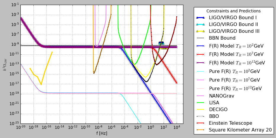
Figure 1: The $h^{2}$-scaled gravitational wave energy spectrum for the combined $F(R)$ gravity kinetic scalar theory versus the sensitivity curves of future gravitational waves experiments. Three distinct reheating temperatures are considered.

By including the WKB contribution to the energy spectrum of the primordial gravitational waves, the latter takes the following form [46, 66, 67, 69, 58, 59, 88],

$$\Omega_{\rm gw}(f)=e^{-2\mathcal{D}}\times\frac{k^{2}}{12H_{0}^{2}}r\mathcal{P}_{\zeta}(k_{ref})\left(\frac{k}{k_{ref}}\right)^{n_{T}}\left(\frac{\Omega_{m}}{\Omega_{\Lambda}}\right)^{2}\left(\frac{g_{*}(T_{\rm in})}{g_{*0}}\right)\left(\frac{g_{*s0}}{g_{*s}(T_{\rm in})}\right)^{4/3}\left(\overline{\frac{3j_{1}(k\tau_{0})}{k\tau_{0}}}\right)^{2}T_{1}^{2}\left(x_{\rm eq}\right)T_{2}^{2}\left(x_{R}\right)\,,$$

with $k_{ref}=0.002$ Mpc^-1 being the pivot scale of CMB. In order to calculate the integral of Eq. (29), we need to solve numerically the Friedmann equation from redshift zero up to the redshift $z_{f}=10^{12}$. We can calculate directly the integral of Eq. (29), by numerically solving the Friedmann equation using appropriate initial conditions. This integration will also reveal the late-time behavior of the combined $F(R)$ gravity kinetic scalar model, but also the behavior of the scalar field up to a redshift $z_{f}=10^{12}$. In order to do so, we bring the Friedmann equation into an appropriate form by using the following relations,

$$\centering\dot{H}=-H(1+z)H^{\prime}\,,\@add@centering$$ (30)

$$\centering\dot{\phi}=-H(1+z)\phi^{\prime}\,,\@add@centering$$ (31)

$$\centering\ddot{\phi}=H^{2}(1+z)^{2}\phi^{\prime\prime}+H^{2}(1+z)\phi^{\prime}+HH^{\prime}(1+z)^{2}\phi^{\prime}\,,\@add@centering$$ (32)

$$\centering\dot{f}_{R}=\dot{R}f_{RR}+\dot{\phi}f_{R\phi}\,,\@add@centering$$ (33)

$$\centering\dot{R}=6H(1+z)^{2}\left(HH^{\prime\prime}+(H^{\prime})^{2}-\frac{3HH^{\prime}}{1+z}\right)\,.\@add@centering$$ (34)

Also we introduce the statefinder function $y_{H}(z)$ [113, 114, 115],

$$\centering y_{H}=\frac{\rho_{DE}}{\rho_{d0}}\,,\@add@centering$$ (35)

where $\rho_{DE}$ denotes the dark matter energy density and $\rho_{d0}$ stands for the value of density for non-relativistic matter at present day. The dark energy density is,

$$\centering\rho_{DE}=\frac{1}{2}\dot{\phi}^{2}+V+\frac{f_{R}R-f}{2\kappa^{2}}-\frac{3H\dot{f}_{R}}{\kappa^{2}}+\frac{3H^{2}}{\kappa^{2}}(1-f_{R})\,,\@add@centering$$ (36)

and the dark energy pressure is,

$$\centering P_{DE}=-V-24\dot{\xi}H^{3}-8\dot{\xi}H\dot{H}-\frac{f_{R}R-f}{2\kappa^{2}}-\frac{2\dot{H}}{\kappa^{2}}(1-f_{R})\,,\@add@centering$$ (37)

with,

$$\centering\dot{\rho}_{DE}+3H(\rho_{DE}+P_{DE})=0\,.\@add@centering$$ (38)

Thus the Friedmann equation takes the form,

$$\centering\frac{3H^{2}}{\kappa^{2}}=\rho_{(m)}+\rho_{DE}\,,\@add@centering$$ (39)

$$\centering-\frac{2\dot{H}}{\kappa^{2}}=\rho_{(m)}+P_{(m)}+\rho_{DE}+P_{DE}\,,\@add@centering$$ (40)

where $\rho_{(m)}$ and $P_{(m)}$ are the total energy density and total pressure of the perfect matter fluids present. In terms of the statefinder function $y_{H}(z)$, the Hubble rate is written as follows,

$$\centering H^{2}=m_{s}^{2}\left(y_{H}(z)+\frac{\rho_{(m)}}{\rho_{d0}}\right)\,,\@add@centering$$ (41)

with $m_{s}^{2}=\kappa^{2}\frac{\rho_{d0}}{3}=1.87101\cdot 10^{-67}$, while the higher derivatives of the Hubble rate read,

$$\centering HH^{\prime}=\frac{m_{s}^{2}}{2}\left(y_{H}^{\prime}+\frac{\rho_{(m)}^{\prime}}{\rho_{d0}}\right)\,,\@add@centering$$ (42)

$$\centering H^{\prime 2}+HH^{\prime\prime}=\frac{m_{s}^{2}}{2}\left(y_{H}^{\prime\prime}+\frac{\rho_{(m)}^{\prime\prime}}{\rho_{d0}}\right)\,.\@add@centering$$ (43)

Finally, with regard to the dark energy era, the dark energy equation of state parameter $\omega_{DE}$ and the dark energy density parameter $\Omega_{DE}$, they can be expressed in terms of the statefinder function $y_{H}$ as follows [114, 115],

$$\centering\omega_{DE}\@add@centering =-1+\frac{1+z}{3}\frac{d\ln{y_{H}}}{dz} \Omega_{DE} =\frac{y_{H}}{y_{H}+\frac{\rho_{(m)}}{\rho_{d0}}}\,.$$ (44)

Also the initial conditions for the statefinder quantity $y_{H}(z)$ and for the scalar field $\phi(z)$ are the following,

$$y_{H}(0)=\frac{\Lambda}{3\text{ms}^{2}}\,,\,\,\,y_{H}^{\prime}(0)=0,\,\,\,\phi(0)=10^{-16}\,M_{p},\,\,\,\phi^{\prime}(0)=10^{-17}\,M_{p}^{2}\,,$$ (45)

so we start basically from a late-time de Sitter era. The energy density parameter of dark energy at present day is equal to $\Omega_{DE}(0)=0.679335$ and the corresponding dark energy EoS parameter $\omega_{DE}(0)=-1$. Upon solving numerically the Friedmann equation, we obtain the numerical solution for the statefinder function $y_{H}(z)$, and thus we can numerically perform the integration of Eq. (29) and the result of the integration is $\int_{0}^{z_{f}}\frac{a_{M}}{1+z^{\prime}}{\rm dz^{\prime}}\simeq-23$ This leads to a large amplification of the pure $F(R)$ gravity signal, and in Fig. 1 we plot the predicted signal of the combined $F(R)$ gravity kinetic scalar theory, and also the sensitivity curves of the future gravitational waves experiments. Note that our WKB solution is valid for subhorizon modes during reheating and beyond, so the small frequency part of the plot must be disregarded, for frequencies smaller that $f<10^{-10}\,$Hz. In the plot of Fig. 1 we included three distinct reheating temperatures, a high one $T_{R}=10^{12}$GeV (purple curve), an intermediate $T_{R}=10^{7}$GeV (red curve) and a low reheating temperature $T_{R}=10^{2}$GeV (blue curve). From Fig. 1 it is obvious that the signal is detectable from all the future gravitational wave experiments, for the high and intermediate temperatures, except for the low reheating temperature. It is also mentionable that the signal of the theory at hand is somewhat uniform and it leads to a nearly constant $h^{2}$-scaled gravitational wave energy spectrum. This indicates that if the signal corresponding to this class of theories is detected by one experiment, then it will be detected by all experiments and will have the same amplitude and energy spectrum. This feature is of particular importance since it is a characteristic of this class of theories. We shall discuss further possibilities on how to discriminate modified gravity theories by using primordial gravitational waves in the next section. One thing to mention which is somewhat important is that the amplification of the primordial gravitational wave energy spectrum only occurs if the potential is small compared to the kinetic term, but if someone chooses a potential that does not satisfy this condition, or if the potential is trivial, no amplification occurs. The potential must be no trivial and present, but it must be dominated by the kinetic term of the scalar field.

Before closing, we need to mention that in our analysis we did include the most recent constraints imposed by the LIGO/VIRGO collaboration [117], which constrain the energy spectrum of the primordial waves to be $\Omega_{GW}\leq 5.8\times 10^{-9}$ for a flat (frequency independent) gravitational wave background in the frequency range $(20-76.6)$Hz (LIGO VIRGO BOUND I), and also $\Omega_{GW}\leq 3.4\times 10^{-9}$ for a power-law gravitational background with a spectral index of $2/3$ in the frequency range $(20-90.6)$Hz (LIGO VIRGO BOUND II) and furthermore $\Omega_{GW}\leq 3.9\times 10^{-10}$ for a spectral index of $3$, in the frequency range $(20-291.6)$Hz (LIGO VIRGO BOUND III). Also we included the constraints from the BBN [54]. As it can be seen in Fig. 1, the resulting combined $F(R)$ gravity kinetic scalar pass the LIGO/VIRGO bounds I and II and also satisfy the BBN, save the large reheating temperature combined $F(R)$ gravity kinetic scalar model, which is marginally compatible with the BBN constraints and completely incompatible with the LIGO/VIRGO bound III. We also included in our study the pure $F(R)$ gravity cases for three reheating temperatures, see the lower lines in Fig. 1. As it can be seen, the signal is way lower than the sensitivity curves of all the future experiments.

We also need to note that the amplification is sensitive to parameter changes, thus the amplification is model dependent. This shows that there is freedom in the choices of the parameters, however it would generally be difficult to pin-point which model produces a future detected signal. However, with this work we aimed to show that it is possible to have an enhancement in the primordial gravitational wave energy spectrum if one combines a kinetic energy dominated scalar field with $F(R)$ gravity, with the scalar field being some light axion-like particle. Of course, more complicated scenarios can occur, for example a complication may be induced by a prolonged inflationary era. This scenario is interesting itself, and is worth studying in the future because the scenario we studied here also leads to a prolonged inflationary era, slightly prolonged though. In conclusion, many features of the standard GR compatible scalar field theory may change when $F(R)$ gravity corrections are taken into account. This work aimed in pointing out this feature of $f(R,\phi)$ theories.

IV Conclusions and Discussion

In this work we studied a combined cosmological framework comprised by an $F(R)$ gravity and a kinetic canonical scalar field. The terminology “kinetic” for the scalar field is used because we assumed that the kinetic energy of the scalar field dominates over its potential for its whole evolution, without however disregarding its potential. Due to the fact that the scalar field is kinetic, this means that during inflation, and of course beyond inflation, the scalar field obeys a constant-roll evolution and it has a stiff equation of state. However, being a stiff fluid, and thus redshifting as $a^{-6}$, this means that it does not affect the inflationary dynamics at the equations of motion level. Nevertheless, we investigated two more ways that this kinetic scalar might affect the dynamics of inflation, one way is at the cosmological perturbations level, via the second slow-roll parameter, and the other way is via the extension of the $e$-foldings number for the inflationary era. As we showed, the effects of the kinetic scalar at the cosmological perturbation level cancels in the final functional form of the observational indices and specifically of the spectral index of the scalar curvature perturbations. On the other hand, the kinetic scalar affects the duration of inflation. Indeed, when the unstable quasi-de Sitter attractor of the $F(R)$ gravity model is reached, the $F(R)$ gravity no longer controls the evolution, thus the kinetic scalar starts to dominate the evolution. This makes the total EoS parameter of the Universe to be equal to unity, thus the Universe passes through a kination era. This feature affects directly the duration of the inflationary era, and thus the observational indices.

After discussing inflation in this kinetic scalar $F(R)$ gravity framework, we investigated the implications of the combined framework on the primordial gravitational wave energy spectrum. Apart from the observational indices of inflation, and specifically the tensor-to-scalar ratio and the tensor spectral index, which are different for the combined $F(R)$ gravity kinetic scalar framework compared to the vacuum $F(R)$ gravity case, the energy spectrum of the former is significantly enhanced compared to the latter theory. We numerically calculated the amplification factor for the combined $F(R)$ gravity kinetic scalar framework, starting from the present day epoch up to redshifts of the order $10^{12}$ which is deeply in the radiation domination era. As we showed, the energy spectrum of the primordial gravitational wave is significantly enhanced and moreover the signal is flat and appears to be of the same order for a wide range of frequencies. A notable feature of the calculation is the form of the potential, and this enhancement seems to work only for potentials that tend to zero for all scalar field values, such as the exponential potentials. It is remarkable though that if we switch off the potential, the enhancement mechanism does not work. One needs a kinetic scalar field with a non-trivial scalar potential which goes smoothly to zero for large scalar field values. Quadratic potentials and in general power-law potentials with positive values of the exponents do not work. Another important feature of this framework is the form of the signal. It has the same form as the vacuum $F(R)$ gravity case, although significantly enhanced. Thus, this class of theories leads to a signal that will be detectable from all the future gravitational wave experiments, if the reheating temperature is large enough though. Hence, if a signal is detected and the signal is of the same order of magnitude for all the detectors, the underlying theory is very likely some sort of combined scalar field $F(R)$ gravity theory, with the amplification mechanism we showed in this article. If however the signal is detected by some and not all the detectors, this would either indicate that the underlying theory is not of the form we discussed in this paper, or there is a strong damping mechanism in specific frequency range. Regarding the latter damping, it is interesting to note there exist various damping mechanisms, for example supersymmetry breaking during reheating, or even the chameleon mechanism may lead to a serious suppression of the energy spectrum, see for example [118]. Thus the future is highly anticipated by theoretical physicists to answer (hopefully) their deep and unanswered for decades questions.

References

- [1] K. N. Abazajian et al. [CMB-S4], [arXiv:1610.02743 [astro-ph.CO]].
- [2] M. H. Abitbol et al. [Simons Observatory], Bull. Am. Astron. Soc. 51 (2019), 147 [arXiv:1907.08284 [astro-ph.IM]].
- [3] S. Hild, M. Abernathy, F. Acernese, P. Amaro-Seoane, N. Andersson, K. Arun, F. Barone, B. Barr, M. Barsuglia and M. Beker, et al. Class. Quant. Grav. 28 (2011), 094013 doi:10.1088/0264-9381/28/9/094013 [arXiv:1012.0908 [gr-qc]].
- [4] J. Baker, J. Bellovary, P. L. Bender, E. Berti, R. Caldwell, J. Camp, J. W. Conklin, N. Cornish, C. Cutler and R. DeRosa, et al. [arXiv:1907.06482 [astro-ph.IM]].
- [5] T. L. Smith and R. Caldwell, Phys. Rev. D 100 (2019) no.10, 104055 doi:10.1103/PhysRevD.100.104055 [arXiv:1908.00546 [astro-ph.CO]].
- [6] J. Crowder and N. J. Cornish, Phys. Rev. D 72 (2005), 083005 doi:10.1103/PhysRevD.72.083005 [arXiv:gr-qc/0506015 [gr-qc]].
- [7] T. L. Smith and R. Caldwell, Phys. Rev. D 95 (2017) no.4, 044036 doi:10.1103/PhysRevD.95.044036 [arXiv:1609.05901 [gr-qc]].
- [8] N. Seto, S. Kawamura and T. Nakamura, Phys. Rev. Lett. 87 (2001), 221103 doi:10.1103/PhysRevLett.87.221103 [arXiv:astro-ph/0108011 [astro-ph]].
- [9] S. Kawamura, M. Ando, N. Seto, S. Sato, M. Musha, I. Kawano, J. Yokoyama, T. Tanaka, K. Ioka and T. Akutsu, et al. [arXiv:2006.13545 [gr-qc]].
- [10] A. Weltman, P. Bull, S. Camera, K. Kelley, H. Padmanabhan, J. Pritchard, A. Raccanelli, S. Riemer-Sørensen, L. Shao and S. Andrianomena, et al. Publ. Astron. Soc. Austral. 37 (2020), e002 doi:10.1017/pasa.2019.42 [arXiv:1810.02680 [astro-ph.CO]].
- [11] P. Auclair et al. [LISA Cosmology Working Group], [arXiv:2204.05434 [astro-ph.CO]].
- [12] A. D. Linde, Lect. Notes Phys. 738 (2008) 1 [arXiv:0705.0164 [hep-th]].
- [13] D. S. Gorbunov and V. A. Rubakov, “Introduction to the theory of the early universe: Cosmological perturbations and inflationary theory,” Hackensack, USA: World Scientific (2011) 489 p;
- [14] A. Linde, arXiv:1402.0526 [hep-th];
- [15] D. H. Lyth and A. Riotto, Phys. Rept. 314 (1999) 1 [hep-ph/9807278].
- [16] S. Nojiri, S. D. Odintsov and V. K. Oikonomou, Phys. Rept. 692 (2017) 1 [arXiv:1705.11098 [gr-qc]].
-
[17]
S. Capozziello, M. De Laurentis,
Phys. Rept. 509, 167 (2011);
V. Faraoni and S. Capozziello, Fundam. Theor. Phys. 170 (2010). - [18] S. Nojiri, S.D. Odintsov, eConf C0602061, 06 (2006) [Int. J. Geom. Meth. Mod. Phys. 4, 115 (2007)].
- [19] S. Nojiri, S.D. Odintsov, Phys. Rept. 505, 59 (2011);
- [20] G. J. Olmo, Int. J. Mod. Phys. D 20 (2011) 413 [arXiv:1101.3864 [gr-qc]].
- [21] S. Nojiri and S. D. Odintsov, Phys. Rev. D 68 (2003), 123512 doi:10.1103/PhysRevD.68.123512 [arXiv:hep-th/0307288 [hep-th]].
- [22] S. Capozziello, V. F. Cardone and A. Troisi, Phys. Rev. D 71 (2005), 043503 doi:10.1103/PhysRevD.71.043503 [arXiv:astro-ph/0501426 [astro-ph]].
- [23] J. c. Hwang and H. Noh, Phys. Lett. B 506 (2001), 13-19 doi:10.1016/S0370-2693(01)00404-X [arXiv:astro-ph/0102423 [astro-ph]].
- [24] G. Cognola, E. Elizalde, S. Nojiri, S. D. Odintsov and S. Zerbini, JCAP 02 (2005), 010 doi:10.1088/1475-7516/2005/02/010 [arXiv:hep-th/0501096 [hep-th]].
- [25] Y. S. Song, W. Hu and I. Sawicki, Phys. Rev. D 75 (2007), 044004 doi:10.1103/PhysRevD.75.044004 [arXiv:astro-ph/0610532 [astro-ph]].
- [26] T. Faulkner, M. Tegmark, E. F. Bunn and Y. Mao, Phys. Rev. D 76 (2007), 063505 doi:10.1103/PhysRevD.76.063505 [arXiv:astro-ph/0612569 [astro-ph]].
- [27] G. J. Olmo, Phys. Rev. D 75 (2007), 023511 doi:10.1103/PhysRevD.75.023511 [arXiv:gr-qc/0612047 [gr-qc]].
- [28] I. Sawicki and W. Hu, Phys. Rev. D 75 (2007), 127502 doi:10.1103/PhysRevD.75.127502 [arXiv:astro-ph/0702278 [astro-ph]].
- [29] V. Faraoni, Phys. Rev. D 75 (2007), 067302 doi:10.1103/PhysRevD.75.067302 [arXiv:gr-qc/0703044 [gr-qc]].
- [30] S. Carloni, P. K. S. Dunsby and A. Troisi, Phys. Rev. D 77 (2008), 024024 doi:10.1103/PhysRevD.77.024024 [arXiv:0707.0106 [gr-qc]].
- [31] S. Nojiri and S. D. Odintsov, Phys. Lett. B 657 (2007), 238-245 doi:10.1016/j.physletb.2007.10.027 [arXiv:0707.1941 [hep-th]].
- [32] N. Deruelle, M. Sasaki and Y. Sendouda, Prog. Theor. Phys. 119 (2008), 237-251 doi:10.1143/PTP.119.237 [arXiv:0711.1150 [gr-qc]].
- [33] S. A. Appleby and R. A. Battye, JCAP 05 (2008), 019 doi:10.1088/1475-7516/2008/05/019 [arXiv:0803.1081 [astro-ph]].
- [34] P. K. S. Dunsby, E. Elizalde, R. Goswami, S. Odintsov and D. S. Gomez, Phys. Rev. D 82 (2010), 023519 doi:10.1103/PhysRevD.82.023519 [arXiv:1005.2205 [gr-qc]].
- [35] S. A. Appleby, R. A. Battye and A. A. Starobinsky, JCAP 1006 (2010) 005 [arXiv:0909.1737 [astro-ph.CO]].
- [36] J. c. Hwang and H. Noh, Phys. Rev. D 71 (2005) 063536 doi:10.1103/PhysRevD.71.063536 [gr-qc/0412126].
- [37] S. D. Odintsov and V. K. Oikonomou, Phys. Lett. B 807 (2020), 135576 doi:10.1016/j.physletb.2020.135576 [arXiv:2005.12804 [gr-qc]].
- [38] V. K. Oikonomou, Phys. Rev. D 106 (2022) no.4, 044041 doi:10.1103/PhysRevD.106.044041 [arXiv:2208.05544 [gr-qc]].
- [39] P. Adshead, R. Easther, J. Pritchard and A. Loeb, JCAP 02 (2011), 021 doi:10.1088/1475-7516/2011/02/021 [arXiv:1007.3748 [astro-ph.CO]].
- [40] J. B. Munoz and M. Kamionkowski, Phys. Rev. D 91 (2015) no.4, 043521 doi:10.1103/PhysRevD.91.043521 [arXiv:1412.0656 [astro-ph.CO]].
- [41] A. R. Liddle and S. M. Leach, Phys. Rev. D 68 (2003), 103503 doi:10.1103/PhysRevD.68.103503 [arXiv:astro-ph/0305263 [astro-ph]].
- [42] T. Hasegawa, N. Hiroshima, K. Kohri, R. S. L. Hansen, T. Tram and S. Hannestad, JCAP 12 (2019), 012 doi:10.1088/1475-7516/2019/12/012 [arXiv:1908.10189 [hep-ph]].
- [43] M. Kamionkowski and E. D. Kovetz, Ann. Rev. Astron. Astrophys. 54 (2016), 227-269 doi:10.1146/annurev-astro-081915-023433 [arXiv:1510.06042 [astro-ph.CO]].
- [44] M. Denissenya and E. V. Linder, JCAP 11 (2018), 010 doi:10.1088/1475-7516/2018/11/010 [arXiv:1808.00013 [astro-ph.CO]].
- [45] M. S. Turner, M. J. White and J. E. Lidsey, Phys. Rev. D 48 (1993), 4613-4622 doi:10.1103/PhysRevD.48.4613 [arXiv:astro-ph/9306029 [astro-ph]].
- [46] L. A. Boyle and P. J. Steinhardt, Phys. Rev. D 77 (2008), 063504 doi:10.1103/PhysRevD.77.063504 [arXiv:astro-ph/0512014 [astro-ph]].
- [47] Y. Zhang, Y. Yuan, W. Zhao and Y. T. Chen, Class. Quant. Grav. 22 (2005), 1383-1394 doi:10.1088/0264-9381/22/7/011 [arXiv:astro-ph/0501329 [astro-ph]].
- [48] B. F. Schutz and F. Ricci, [arXiv:1005.4735 [gr-qc]].
- [49] B. S. Sathyaprakash and B. F. Schutz, Living Rev. Rel. 12 (2009), 2 doi:10.12942/lrr-2009-2 [arXiv:0903.0338 [gr-qc]].
- [50] C. Caprini and D. G. Figueroa, Class. Quant. Grav. 35 (2018) no.16, 163001 doi:10.1088/1361-6382/aac608 [arXiv:1801.04268 [astro-ph.CO]].
- [51] G. Arutyunov, M. Heinze and D. Medina-Rincon, J. Phys. A 50 (2017) no.24, 244002 doi:10.1088/1751-8121/aa6e0c [arXiv:1608.06481 [hep-th]].
- [52] S. Kuroyanagi, T. Chiba and N. Sugiyama, Phys. Rev. D 79 (2009), 103501 doi:10.1103/PhysRevD.79.103501 [arXiv:0804.3249 [astro-ph]].
- [53] T. J. Clarke, E. J. Copeland and A. Moss, JCAP 10 (2020), 002 doi:10.1088/1475-7516/2020/10/002 [arXiv:2004.11396 [astro-ph.CO]].
- [54] S. Kuroyanagi, T. Takahashi and S. Yokoyama, JCAP 02 (2015), 003 doi:10.1088/1475-7516/2015/02/003 [arXiv:1407.4785 [astro-ph.CO]].
- [55] K. Nakayama and J. Yokoyama, JCAP 01 (2010), 010 doi:10.1088/1475-7516/2010/01/010 [arXiv:0910.0715 [astro-ph.CO]].
- [56] T. L. Smith, M. Kamionkowski and A. Cooray, Phys. Rev. D 73 (2006), 023504 doi:10.1103/PhysRevD.73.023504 [arXiv:astro-ph/0506422 [astro-ph]].
- [57] M. Giovannini, Class. Quant. Grav. 26 (2009), 045004 doi:10.1088/0264-9381/26/4/045004 [arXiv:0807.4317 [astro-ph]].
- [58] X. J. Liu, W. Zhao, Y. Zhang and Z. H. Zhu, Phys. Rev. D 93 (2016) no.2, 024031 doi:10.1103/PhysRevD.93.024031 [arXiv:1509.03524 [astro-ph.CO]].
- [59] W. Zhao, Y. Zhang, X. P. You and Z. H. Zhu, Phys. Rev. D 87 (2013) no.12, 124012 doi:10.1103/PhysRevD.87.124012 [arXiv:1303.6718 [astro-ph.CO]].
- [60] S. Vagnozzi, Mon. Not. Roy. Astron. Soc. 502 (2021) no.1, L11-L15 doi:10.1093/mnrasl/slaa203 [arXiv:2009.13432 [astro-ph.CO]].
- [61] Y. Watanabe and E. Komatsu, Phys. Rev. D 73 (2006), 123515 doi:10.1103/PhysRevD.73.123515 [arXiv:astro-ph/0604176 [astro-ph]].
- [62] M. Kamionkowski, A. Kosowsky and M. S. Turner, Phys. Rev. D 49 (1994), 2837-2851 doi:10.1103/PhysRevD.49.2837 [arXiv:astro-ph/9310044 [astro-ph]].
- [63] W. Giarè and F. Renzi, Phys. Rev. D 102 (2020) no.8, 083530 doi:10.1103/PhysRevD.102.083530 [arXiv:2007.04256 [astro-ph.CO]].
- [64] S. Kuroyanagi, T. Takahashi and S. Yokoyama, JCAP 01 (2021), 071 doi:10.1088/1475-7516/2021/01/071 [arXiv:2011.03323 [astro-ph.CO]].
- [65] W. Zhao and Y. Zhang, Phys. Rev. D 74 (2006), 043503 doi:10.1103/PhysRevD.74.043503 [arXiv:astro-ph/0604458 [astro-ph]].
- [66] A. Nishizawa, Phys. Rev. D 97 (2018) no.10, 104037 doi:10.1103/PhysRevD.97.104037 [arXiv:1710.04825 [gr-qc]].
- [67] S. Arai and A. Nishizawa, Phys. Rev. D 97 (2018) no.10, 104038 doi:10.1103/PhysRevD.97.104038 [arXiv:1711.03776 [gr-qc]].
- [68] E. Bellini and I. Sawicki, JCAP 07 (2014), 050 doi:10.1088/1475-7516/2014/07/050 [arXiv:1404.3713 [astro-ph.CO]].
- [69] R. C. Nunes, M. E. S. Alves and J. C. N. de Araujo, Phys. Rev. D 99 (2019) no.8, 084022 doi:10.1103/PhysRevD.99.084022 [arXiv:1811.12760 [gr-qc]].
- [70] R. D’Agostino and R. C. Nunes, Phys. Rev. D 100 (2019) no.4, 044041 doi:10.1103/PhysRevD.100.044041 [arXiv:1907.05516 [gr-qc]].
- [71] A. Mitra, J. Mifsud, D. F. Mota and D. Parkinson, Mon. Not. Roy. Astron. Soc. 502 (2021) no.4, 5563-5575 doi:10.1093/mnras/stab165 [arXiv:2010.00189 [astro-ph.CO]].
- [72] S. Kuroyanagi, K. Nakayama and S. Saito, Phys. Rev. D 84 (2011), 123513 doi:10.1103/PhysRevD.84.123513 [arXiv:1110.4169 [astro-ph.CO]].
- [73] P. Campeti, E. Komatsu, D. Poletti and C. Baccigalupi, JCAP 01 (2021), 012 doi:10.1088/1475-7516/2021/01/012 [arXiv:2007.04241 [astro-ph.CO]].
- [74] A. Nishizawa and H. Motohashi, Phys. Rev. D 89 (2014) no.6, 063541 doi:10.1103/PhysRevD.89.063541 [arXiv:1401.1023 [astro-ph.CO]].
- [75] W. Zhao, Chin. Phys. 16 (2007), 2894-2902 doi:10.1088/1009-1963/16/10/012 [arXiv:gr-qc/0612041 [gr-qc]].
- [76] W. Cheng, T. Qian, Q. Yu, H. Zhou and R. Y. Zhou, Phys. Rev. D 104 (2021) no.10, 103502 doi:10.1103/PhysRevD.104.103502 [arXiv:2107.04242 [hep-ph]].
- [77] A. Nishizawa, K. Yagi, A. Taruya and T. Tanaka, Phys. Rev. D 85 (2012), 044047 doi:10.1103/PhysRevD.85.044047 [arXiv:1110.2865 [astro-ph.CO]].
- [78] S. Chongchitnan and G. Efstathiou, Phys. Rev. D 73 (2006), 083511 doi:10.1103/PhysRevD.73.083511 [arXiv:astro-ph/0602594 [astro-ph]].
- [79] P. D. Lasky, C. M. F. Mingarelli, T. L. Smith, J. T. Giblin, D. J. Reardon, R. Caldwell, M. Bailes, N. D. R. Bhat, S. Burke-Spolaor and W. Coles, et al. Phys. Rev. X 6 (2016) no.1, 011035 doi:10.1103/PhysRevX.6.011035 [arXiv:1511.05994 [astro-ph.CO]].
- [80] M. C. Guzzetti, N. Bartolo, M. Liguori and S. Matarrese, Riv. Nuovo Cim. 39 (2016) no.9, 399-495 doi:10.1393/ncr/i2016-10127-1 [arXiv:1605.01615 [astro-ph.CO]].
- [81] I. Ben-Dayan, B. Keating, D. Leon and I. Wolfson, JCAP 06 (2019), 007 doi:10.1088/1475-7516/2019/06/007 [arXiv:1903.11843 [astro-ph.CO]].
- [82] K. Nakayama, S. Saito, Y. Suwa and J. Yokoyama, JCAP 06 (2008), 020 doi:10.1088/1475-7516/2008/06/020 [arXiv:0804.1827 [astro-ph]].
- [83] S. Capozziello, M. De Laurentis, S. Nojiri and S. D. Odintsov, Phys. Rev. D 95 (2017) no.8, 083524 doi:10.1103/PhysRevD.95.083524 [arXiv:1702.05517 [gr-qc]].
- [84] S. Capozziello, M. De Laurentis, S. Nojiri and S. D. Odintsov, Gen. Rel. Grav. 41 (2009), 2313-2344 doi:10.1007/s10714-009-0758-1 [arXiv:0808.1335 [hep-th]].
- [85] S. Capozziello, C. Corda and M. F. De Laurentis, Phys. Lett. B 669 (2008), 255-259 doi:10.1016/j.physletb.2008.10.001 [arXiv:0812.2272 [astro-ph]].
- [86] R. G. Cai, C. Fu and W. W. Yu, [arXiv:2112.04794 [astro-ph.CO]].
- [87] R. g. Cai, S. Pi and M. Sasaki, Phys. Rev. Lett. 122 (2019) no.20, 201101 doi:10.1103/PhysRevLett.122.201101 [arXiv:1810.11000 [astro-ph.CO]].
- [88] S. D. Odintsov, V. K. Oikonomou and F. P. Fronimos, Phys. Dark Univ. 35 (2022), 100950 doi:10.1016/j.dark.2022.100950 [arXiv:2108.11231 [gr-qc]].
- [89] M. Benetti, L. L. Graef and S. Vagnozzi, Phys. Rev. D 105 (2022) no.4, 043520 doi:10.1103/PhysRevD.105.043520 [arXiv:2111.04758 [astro-ph.CO]].
- [90] J. Lin, S. Gao, Y. Gong, Y. Lu, Z. Wang and F. Zhang, [arXiv:2111.01362 [gr-qc]].
- [91] F. Zhang, J. Lin and Y. Lu, Phys. Rev. D 104 (2021) no.6, 063515 [erratum: Phys. Rev. D 104 (2021) no.12, 129902] doi:10.1103/PhysRevD.104.063515 [arXiv:2106.10792 [gr-qc]].
- [92] S. D. Odintsov and V. K. Oikonomou, Phys. Lett. B 824 (2022), 136817 doi:10.1016/j.physletb.2021.136817 [arXiv:2112.02584 [gr-qc]].
- [93] J. R. Pritchard and M. Kamionkowski, Annals Phys. 318 (2005), 2-36 doi:10.1016/j.aop.2005.03.005 [arXiv:astro-ph/0412581 [astro-ph]].
- [94] Y. Zhang, W. Zhao, T. Xia and Y. Yuan, Phys. Rev. D 74 (2006), 083006 doi:10.1103/PhysRevD.74.083006 [arXiv:astro-ph/0508345 [astro-ph]].
- [95] D. Baskaran, L. P. Grishchuk and A. G. Polnarev, Phys. Rev. D 74 (2006), 083008 doi:10.1103/PhysRevD.74.083008 [arXiv:gr-qc/0605100 [gr-qc]].
- [96] V. K. Oikonomou, Astropart. Phys. 141 (2022), 102718 doi:10.1016/j.astropartphys.2022.102718 [arXiv:2204.06304 [gr-qc]].
- [97] S. D. Odintsov, V. K. Oikonomou and R. Myrzakulov, Symmetry 14 (2022) no.4, 729 doi:10.3390/sym14040729 [arXiv:2204.00876 [gr-qc]].
- [98] S. D. Odintsov and V. K. Oikonomou, [arXiv:2203.10599 [gr-qc]].
- [99] S. Kawai and J. Kim, Phys. Lett. B 789, 145-149 (2019) [arXiv:1702.07689 [hep-th]].
- [100] S. D. Odintsov and V. K. Oikonomou, [arXiv:2205.07304 [gr-qc]].
- [101] X. Gao and X. Y. Hong, Phys. Rev. D 101 (2020) no.6, 064057 doi:10.1103/PhysRevD.101.064057 [arXiv:1906.07131 [gr-qc]].
- [102] V. K. Oikonomou and E. C. Lymperiadou, [arXiv:2206.00721 [gr-qc]].
- [103] V. K. Oikonomou, [arXiv:2205.15405 [gr-qc]].
- [104] S. Vagnozzi and A. Loeb, [arXiv:2208.14088 [astro-ph.CO]].
- [105] M. Gerbino, K. Freese, S. Vagnozzi, M. Lattanzi, O. Mena, E. Giusarma and S. Ho, Phys. Rev. D 95 (2017) no.4, 043512 doi:10.1103/PhysRevD.95.043512 [arXiv:1610.08830 [astro-ph.CO]].
- [106] A. Casalino, M. Rinaldi, L. Sebastiani and S. Vagnozzi, Class. Quant. Grav. 36 (2019) no.1, 017001 doi:10.1088/1361-6382/aaf1fd [arXiv:1811.06830 [gr-qc]].
- [107] A. Casalino, M. Rinaldi, L. Sebastiani and S. Vagnozzi, Phys. Dark Univ. 22 (2018), 108 doi:10.1016/j.dark.2018.10.001 [arXiv:1803.02620 [gr-qc]].
- [108] L. Visinelli, N. Bolis and S. Vagnozzi, Phys. Rev. D 97 (2018) no.6, 064039 doi:10.1103/PhysRevD.97.064039 [arXiv:1711.06628 [gr-qc]].
- [109] L. Visinelli and S. Vagnozzi, Phys. Rev. D 99 (2019) no.6, 063517 doi:10.1103/PhysRevD.99.063517 [arXiv:1809.06382 [hep-ph]].
- [110] W. H. Kinney, S. Vagnozzi and L. Visinelli, Class. Quant. Grav. 36 (2019) no.11, 117001 doi:10.1088/1361-6382/ab1d87 [arXiv:1808.06424 [astro-ph.CO]].
- [111] W. Giarè, F. Renzi and A. Melchiorri, Phys. Rev. D 103 (2021) no.4, 043515 doi:10.1103/PhysRevD.103.043515 [arXiv:2012.00527 [astro-ph.CO]].
- [112] A. Ricciardone, J. Phys. Conf. Ser. 840 (2017) no.1, 012030 doi:10.1088/1742-6596/840/1/012030 [arXiv:1612.06799 [astro-ph.CO]].
- [113] W. Hu and I. Sawicki, Phys. Rev. D 76 (2007), 064004 doi:10.1103/PhysRevD.76.064004 [arXiv:0705.1158 [astro-ph]].
- [114] K. Bamba, A. Lopez-Revelles, R. Myrzakulov, S. D. Odintsov and L. Sebastiani, Class. Quant. Grav. 30 (2013) 015008 doi:10.1088/0264-9381/30/1/015008 [arXiv:1207.1009 [gr-qc]].
- [115] S. D. Odintsov, V. K. Oikonomou and F. P. Fronimos, Phys. Dark Univ. 29 (2020), 100563 doi:10.1016/j.dark.2020.100563 [arXiv:2004.08884 [gr-qc]].
- [116] M. Breitbach, J. Kopp, E. Madge, T. Opferkuch and P. Schwaller, JCAP 07 (2019), 007 doi:10.1088/1475-7516/2019/07/007 [arXiv:1811.11175 [hep-ph]].
- [117] R. Abbott et al. [KAGRA, Virgo and LIGO Scientific], Phys. Rev. D 104 (2021) no.2, 022004 doi:10.1103/PhysRevD.104.022004 [arXiv:2101.12130 [gr-qc]].
- [118] T. Katsuragawa, T. Nakamura, T. Ikeda and S. Capozziello, Phys. Rev. D 99 (2019) no.12, 124050 doi:10.1103/PhysRevD.99.124050 [arXiv:1902.02494 [gr-qc]].