Brownian non-Gaussian diffusion of self-avoiding walks

Abstract

Three-dimensional Monte Carlo simulations provide a striking confirmation to a recent theoretical prediction: the Brownian non-Gaussian diffusion of critical self-avoiding walks. Although the mean square displacement of the polymer center of mass grows linearly with time (Brownian behavior), the initial probability density function is strongly non-Gaussian and crosses over to Gaussianity only at large time. Full agreement between theory and simulations is achieved without the employment of fitting parameters. We discuss simulation techniques potentially capable of addressing the study of anomalous diffusion under complex conditions like adsorption- or Theta-transition.

Keywords: Anomalous diffusion, Polymers, Critical phenomena

1 Introduction

A wealth of recent experiments [1, 2, 3, 4, 5, 6, 7, 8, 9, 10, 11, 12, 13, 14, 15, 16, 17, 18] and molecular dynamics simulations [19, 20, 21] highlighted the existence of diffusion processes in which the mean square displacement linearly grows in time (in agreement with Brownian behavior), but the probability density function (PDF) of the tracer displacement is non-Gaussian during long stages. This has triggered interest for the introduction of novel mesoscopic models relying on superposition of statistics [22, 23, 17, 2], diffusing diffusivities [24, 25, 26, 27, 28, 29, 30], continuous time random walk [31, 32, 33], and diffusion in disordered environments [34], as well as theoretical approaches based on a clear microscopic foundation [35, 36, 37, 38]. A simple microscopic prototype displaying Brownian non-Gaussian diffusion is represented by a tracer undergoing conformational modifications which affect its diffusion coefficient. Consider for instance the centre of mass (CM) of a polymer in contact with a chemostat, so that its size $N$ may fluctuate as it does in the grand canonical ensemble. Since the CM diffusion coefficient is a function of the size, size fluctuations naturally generate diffusivity fluctuations and this renders the initial PDF of the CM displacement non-Gaussian (see below). Importantly, the phenomenon becomes evident close to the polymer critical point separating the dilute from the dense phase [39, 40, 41, 42], where size fluctuations diverge and the behaviour becomes universal, only depending on the spatial dimension $d$, on the polymer topology, and the solvent conditions. This state of affairs has been recently theorised in Refs. [36, 37], where explicit predictions about the initial PDF shape have been made based on the critical exponents characterising the polymer universality class.

By exploiting the fact that a microscopic model is endowed with its own independent dynamics, here we consider grand canonical (i.e. $N$ varying) simulations of the three-dimensional ($d=3$) self-avoiding walks (SAW) on the cubic lattice as a model for a linear polymer fluctuating in size under good solvent conditions [41]. The use of Monte Carlo SAW schemes to simulate polymer dynamics dates back to the work of Baumgartner and Binder [43], where it was implemented the so-called “kink-jump dynamics”. Since then, many processes involving polymer dynamics have been simulated via the use of Monte Carlo methods (see for instance Refs. [44, 45]). Although these schemes do not fully mimic Netwonian dynamics – e.g., they disregards inertial effects – in many cases they faithfully describe the diffusion properties of the system and allow for massive statistical sampling with respect to the molecular dynamics counterparts. The algorithm outlined in Section 3, based on a variant of the “kink-jump” suitable for SAWs on a cubic lattice, will be shown to correctly reproduce the polymer diffusion dynamics. After reviewing the universality class of three-dimensional SAWs, we address the CM displacements during the simulation dynamics and show a striking agreement between the corresponding PDF and the theoretical predictions reported in Refs. [36, 37]. Importantly, this conformity is achieved without employing any fitting parameter and provides a standalone microscopic validation for the Brownian non-Gaussian character of the CM motion of polymers in proximity of their critical point.

The paper is organised as follows. In the next Section we provide the theoretical background for three-dimensional SAWs and for the diffusion properties of their CM. We then supply details of the simulation methods and end the paper by a discussion of our results and future developments.

2 Theoretical background

SAWs are a fundamental mathematical model employed to reproduce the properties of linear polymers in good solvent [41]. Assuming for simplicity the same energy for all SAWs, their equilibrium statistical behaviour in the grand canonical ensemble is described by the partition (or generating) function

$$Z_{\mathrm{gc}}(z)=\sum_{n}c_{n}\,z^{n}\,,=\sum_{\omega}z^{|\omega|}\,,$$ (1)

where $c_{n}$ is the number of distinct $n$-step SAWs, and $z$ the step fugacity; the second sum is over all SAWs $\omega$, of arbitrary size $|\omega|$. In the grand canonical ensemble, the fugacity $z=\mathrm{e}^{\mu/k_{\mathrm{B}}T}$ (where $\mu$ is the chemical potential, $T$ temperature, and $k_{\mathrm{B}}$ the Boltzmann constant) corresponds to an intensive thermodynamic variable controlling the interchanges of particles between the system and the chemostat; for SAWs, added and removed particles amount to added and removed steps. It is well known that a model-dependent critical fugacity $z_{\mathrm{c}}$ separates the dilute polymer phase in which the average size $\mathbb{E}[N]$ is finite from a dense one characterized by a divergent $\mathbb{E}[N]$; with a three-dimensional cubic lattice critical fugacity, $z_{\mathrm{c}}\simeq 0.213490$ [46]. As $z\to z_{\mathrm{c}}^{-}$ the partition function takes the universal form

$$Z_{\mathrm{gc}}(z)=\sum_{n=n_{\mathrm{min}}}^{\infty}(z/z_{\mathrm{c}})^{n}\,n^{\gamma-1}=\mathrm{Li}_{1-\gamma}(z/z_{\mathrm{c}})-\sum_{n=1}^{n_{\mathrm{min}}}(z/z_{\mathrm{c}})^{n}\,n^{\gamma-1}\sim(1-z/z_{\mathrm{c}})^{-\gamma}\,,$$ (2)

where $\gamma$ is the critical entropic exponent whose estimate in $d=3$ is $\gamma=1.15695300(95)$ [47], and $\mathrm{Li}_{s}(z)\equiv\sum_{n=1}^{\infty}z^{n}/n^{s}$ the polylogarithm function. In Eq. (2) we have assumed a minimal number of steps $n_{\mathrm{min}}$, which will be discussed below.

If we now consider SAWs of fixed size $N=n\geq n_{\mathrm{min}}$, from one hand Eq. (2) tells that their equilibrium occurrence is given by the probability distribution

$$P_{N}^{*}(n)=\dfrac{(z/z_{\mathrm{c}})^{n}\;n^{\gamma-1}}{Z_{\mathrm{gc}}(z)}\sim(1-z/z_{\mathrm{c}})^{\gamma}\;(z/z_{\mathrm{c}})^{n}\;n^{\gamma-1}\,.$$ (3)

On the other hand, random conformational changes of these SAWs induce a diffusive motion for the position $\bm{R}_{\mathrm{CM}}(t)=(X_{\mathrm{CM}}(t),Y_{\mathrm{CM}}(t),Z_{\mathrm{CM}}(t))$ of their CM according to

$$\mathrm{d}\bm{R}_{\mathrm{CM}}(t)=\sqrt{2D(n)}\,\mathrm{d}\bm{B}(\mathrm{d}t)\,,$$ (4)

with $\bm{B}(\mathrm{d}t)$ being a Wiener process (Brownian motion) and $D(n)$ the corresponding diffusion coefficient. As explained in the next Section, the stochastic motion of the SAWs is implemented via a kinetic Monte Carlo with local deformations on the lattice. As a consequence, hydrodynamic effects are not taken into account by our dynamics and the size-dependency of the diffusion coefficient is expected to be Rouse-like [48], namely

$$D(n)\simeq\dfrac{D_{\mathrm{m}}}{n}\,,$$ (5)

for sufficiently large $n$’s and $D_{\mathrm{m}}$ being an effective single-monomer diffusion coefficient. Figure 1 confirms this expectation.

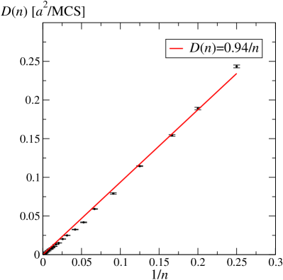
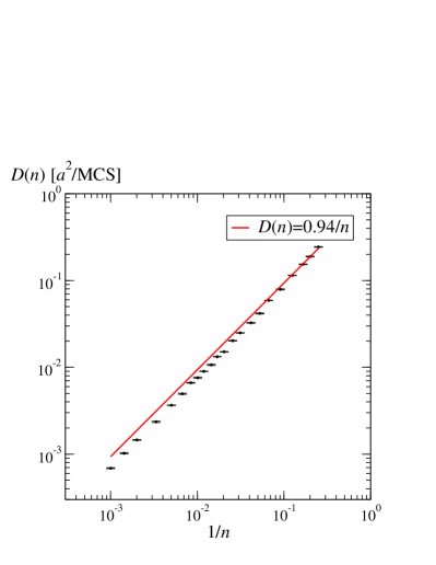
Figure 1: CM diffusion coefficient for fixed size $n\geq 4$ SAWs in a cubic lattice of constant $a$, both in linear and log-log scale. Symbols: $D(n)$ is measured in units of $a^{2}$ over Monte Carlo Steps (MCS) – see Section 3.1 for the description of $n$-preserving Monte Carlo moves. Line: null-intercept linear regression yielding $D_{\mathrm{m}}=0.94\;a^{2}/\mathrm{MCS}$ in Eq. (5), with regression coefficient $r=0.9991$.

Coming back to the grand canonical ensemble, size fluctuations may be described in terms of a birth-death process $N(t)$ [36, 37]:

$$\begin{array}[]{ll}\partial_{t}P_{N}(n,t|n_{0})=&\mu\,P_{N}(n+1,t|n_{0})+\lambda(n-1)\,P_{N}(n-1,t|n_{0})\vspace{0.1cm}\\ &-(\mu+\lambda(n))P_{N}(n,t|n_{0})\qquad\qquad\;\;\;\;(n>n_{\mathrm{min}})\vspace{0.1cm}\\ \partial_{t}P_{N}(n_{\mathrm{min}},t|n_{0})=&\mu\,P_{N}(n_{\mathrm{min}}+1,t|n_{0})-\lambda(n_{\mathrm{min}})\,P_{N}(n_{\mathrm{min}},t|n_{0})\end{array}$$ (6)

where $\lambda(n)$ and $\mu$ are respectively the association and dissociation rates. Here, $P_{N}(n,t|n_{0})$ is the probability for $N(t)=n$, given $N(0)=n_{0}$. Calling $\tau$ the autocorrelation time of $N(t)$, the expected asymptotic behaviours for $P_{N}(n,t|n_{0})$ are $P_{N}(n,t|n_{0})\begin{subarray}{c}\sim\\ t\ll\tau\end{subarray}\delta_{n,n_{0}}$ and $P_{N}(n,t|n_{0})\begin{subarray}{c}\sim\\ t\gg\tau\end{subarray}P^{\star}_{N}(n)$. Note that we have assumed the dissociation rate to be independent of the size $n$, since it typically represents a decay process occurring at the extremities of the chain. Conversely, the detail balance condition applied to the equilibrium distribution straightforwardly yields [37]

$$\lambda(n)=\mu\,\dfrac{P^{\star}_{N}(n+1)}{P^{\star}_{N}(n)}=\mu\,\dfrac{z}{z_{\mathrm{c}}}\,\left(\dfrac{n+1}{n}\right)^{\gamma-1}\,.$$ (7)

In what follows $\mu$, with the dimension of an inverse time, can be regarded as a free parameter which may be tuned to match the model with the autocorrelation $\tau$ of real physical conditions [37].

A fluctuating $N(t)$ adds a second source of randomness to Eq. (4); in the literature, $N(t)$ is called the subordinator and $\bm{B}(t)$ the subordinated process [49, 50]. It is convenient to reparametrize the diffusion path in terms of the coordinate $s\geq 0$, $\mathrm{d}s=2\,D(n(t))\,\mathrm{d}t$, corresponding to the realization of the stochastic process

$$S(t)\equiv 2\int_{0}^{t}\mathrm{d}t^{\prime}\,D(N(t^{\prime}))=2D_{\mathrm{m}}\int_{0}^{t}\mathrm{d}t^{\prime}\,N^{-1}(t^{\prime})\,,$$ (8)

with PDF $p_{S}(s,t|n_{0})$. The conditional PDF for the CM displacement $\bm{R}_{\mathrm{CM}}=\bm{r}$ at time $t$ given the initial conditions $N=n_{0}$, $\bm{R}_{\mathrm{CM}}=\bm{0}$ at time $0$, $p_{\bm{R}_{\mathrm{CM}}}(\bm{r},t|n_{0};\bm{0})$, is then obtained through the subordination formula [25, 36, 37]

$$p_{\bm{R}_{\mathrm{CM}}}(\bm{r},t|n_{0};\bm{0})=\int_{0}^{\infty}\mathrm{d}s\,\dfrac{\mathrm{e}^{-\frac{\bm{r}^{2}}{2s}}}{(2\pi\,s)^{3/2}}\;p_{S}(s,t|n_{0})\,.$$ (9)

Taking an equilibrium distribution $P^{\star}_{N}(n_{0})$ for the initial sizes of the SAW, from Eq. (9) one gets the Brownian character of the CM diffusion:

$$\mathbb{E}\left[\bm{R}_{\mathrm{CM}}^{2}(t)\right]=3\,\mathbb{E}\left[S(t)\right]=6\,D_{\mathrm{av}}\,t\,,$$ (10)

with $D_{\mathrm{av}}\equiv\displaystyle\sum_{n=n_{\mathrm{min}}}^{\infty}\dfrac{D_{\mathrm{m}}}{n}\,P^{\star}_{N}(n)$. The shape of the initial non-Gaussian PDF for the polymer CM is instead conveniently studied by switching to the unit-variance dimensionless variable $\overline{X}_{\mathrm{CM}}(t)\equiv X_{\mathrm{CM}}(t)/\sqrt{\mathbb{E}[X_{\mathrm{CM}}^{2}(t)]}$. From Eq. (9) and the asymptotic limits of the birth-death process, as $t\to 0^{+}$ we have

$$p_{\overline{X}_{\mathrm{CM}}}(x,0^{+})\simeq\sum_{n=n_{\mathrm{min}}}^{\infty}P^{\star}_{N}(n)\,\dfrac{\mathrm{e}^{-\frac{\mathbb{E}[N^{-1}]\,x^{2}}{2\,n^{-1}}}}{\sqrt{2\pi\,\frac{n^{-1}}{\mathbb{E}[N^{-1}]}}}\,.$$ (11)

At large $|x|$ the PDF is asymptotic to the Gaussian cutoff $\sim\mathrm{e}^{-\mathbb{E}[N^{-1}]\,x^{2}/(2\,n_{\mathrm{min}}^{-1})}$, and as $z/z_{\mathrm{c}}\to 1$ this cutoff is pushed towards $|x|\to\infty$, since $\mathbb{E}[N^{-1}]\to 0$. Conversely, in the long time limit the ordinary Gaussian behavior is restored, $p_{\overline{X}_{\mathrm{CM}}}(x,\infty)\sim\mathrm{e}^{-x^{2}/2}$. The autocorrelation $\tau$ is the time scale separating the two behaviours; as $z\to z_{\mathrm{c}}^{-}$ this autocorrelation time diverges [37] (critical slowing down).

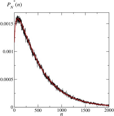
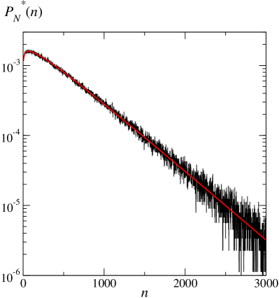
Figure 2: Comparison between the Monte Carlo estimation for $P_{N}^{\star}(n)$ (black line) and Eq. (3) (red line), both in linear and log-linear plot.

3 Simulation methods

On-lattice models are a schematic representation of actual polymers, allowing for massive data sampling. In the present simplification in which all configurations share the same energy, they are particularly effective in reproducing the equilibrium statistics under detail balance conditions. Since we want to sample SAWs in the grand canonical ensemble, we apply a Monte Carlo method based on a variation of the Berretti-Sokal algorithm [51], perhaps the simplest variable-length dynamic Monte Carlo method whose state space is the set of all SAWs (i.e. SAWs on any lengths) in a cubic lattice. The basic idea of the original implementation is that, at each iteration, one of the two ends of the chain is randomly chosen; then, with probability $P_{N}(n-1|n)$ the last step of the walk is deleted (deletion or $-1$ move), while with probability $P_{N}(n+1|n)=1-P_{N}(n-1|n)$ an attempt is made to increase the SAWs length by appending a new edge with equal probability in each of the $2d=6$ possible directions ($+1$ move). In the latter case, if the new configuration is not self-avoiding the proposed move is rejected and the old configuration is counted again in the sampling (null transition). A null transition is also made if a deletion move is attempted on a walk with $n=n_{\mathrm{min}}$ steps. To assure that the invariant probability distribution of a walk is correctly given by $P_{\Omega}^{\star}(\omega)=z^{|\omega|}/Z_{\mathrm{gc}}(z)$, the transition probabilities for the $\pm 1$ moves are taken according to [51]

$$P_{N}(n+1|n)=\frac{2dz}{1+2dz},\qquad P_{N}(n-1|n)=\frac{1}{1+2dz}.$$ (12)

The implementation of this algorithm recovers the estimates of $z_{\mathrm{c}}$ and $\gamma$ given above; in particular, Figure 2 reports a very good agreement between the equilibrium size distribution sampled with the Monte Carlo strategy and Eq. (3). Grand canonical Monte Carlo simulations reported in Figure 2 and in the following ones are performed at $z/z_{\mathrm{c}}=0.997677$; evaluation of the autocorrelation time for this fugacity returns $\tau\simeq\times 10^{6}\;\mathrm{MCS}$.

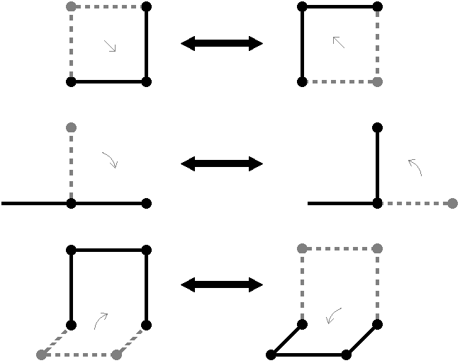
Figure 3: $n$-preserving Monte Carlo moves. For each of the three kind of moves, two reciprocal realizations are plotted.

3.1 Motion of the CM

In order to reproduce the diffusion dynamics of a polymer, the algorithm is enriched by adding three types of $n$-preserving local moves as shown in Figure 3. These are: (i) the one-vertex flip or kink move; (ii) the $90^{\circ}$ rotation of end steps; (iii) the $90^{\circ}$ crankshaft move [52]. In all cases, if the move leads to a violation of self-avoidance, the attempted move is rejected. For a SAW of size $n$, each MCS consists of one attempted Berretti-Sokal move followed by a sequence of $n$ attempts of moves of the kind (i)–(iii) with a random choice of the location and of the specific $n$-preserving move. Since moves of kind (iii) attempt to change the position of two vertices in place of that of a single one, they are proposed with half the probability of moves (i), (ii). Note that for the whole set of three local moves to be potentially applicable, a minimal number of $3$ steps is required; in our simulations we then set $n_{\mathrm{min}}=4$ to have ensured proper mobility at all sizes. This minimal size is still sufficiently small to guarantee the ergodicity of the algorithm [51]. Ergodicity is in fact granted once it is assured the possibility of passing from any $n$-step SAW to any other $n^{\prime}$-step SAW within a finite number of moves ($n_{\mathrm{min}}\leq n,n^{\prime}<\infty$). In view of the reversibility of the moves, this is equivalent to the capability of reaching a specific target (say, e.g., a $4$-step SAW completely straighten along the $x$ direction) from any $n$-step SAW. It is easy to figure out a possible finite sequence of moves performing the last task as follows: first, the application of $n-4$ moves of the kind $-1$ reaches one of the $726$ [53, 54] distinct $4$-step SAWs occurring on the cubic lattice; then, within a finite sequence of $n$-preserving moves the target is certainly reached. In all our simulations for the motion of CM we start from a grand canonical equilibrium configuration.

Eventually, it is interesting to point out that the correct diffusive properties for our polymer model are reproduced even neglecting thermal fluctuations induced by the interaction with the solvent, which might excite translational and rotational degrees of freedom of the polymer. Such a simplification, enabling a larger statistical sampling, is in line with kinetic Monte Carlo standards [43, 44, 45], and is ultimately allowed by the fact that the overdamped motion of the CM is in fact an attractor for a wide class of dynamical models.

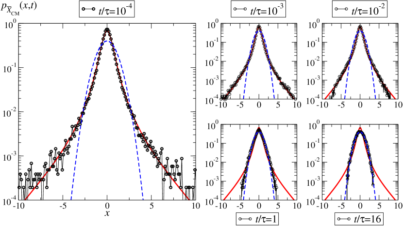
Figure 4: Non-Gaussian diffusion of SAWs. Exact theoretical predictions for the PDF of the unit-variance dimensionless variable $\overline{X}_{\mathrm{CM}}(t)\equiv X_{\mathrm{CM}}(t)/\sqrt{\mathbb{E}[X_{\mathrm{CM}}^{2}(t)]}$ (curves) are compared with normalized displacement histograms obtained from Monte Carlo simulations (circles). With $t/\tau\leq 10^{-2}$, histograms are built with $4.9\times 10^{5}$ realizations; otherwise with $6.6\times 10^{4}$ realizations. Full red lines are given by Eq. (11); dashed blue lines reproduce a zero-mean unit-variance Gaussian.

4 Discussion

According to Eq. (11) the shape of the initial PDF $p_{\overline{X}_{\mathrm{CM}}}(x,0^{+})$ is universal close to criticality, being identified by the value of the fugacity, by $\gamma$, and by the exponent of the $D$-vs-$n$ relation ($-1$ in the present case). The only remaining detail is $n_{\mathrm{min}}$, fixed equal to $4$ in our simulations. Hence, no fitting parameter are left free. Figure. 4 highlights a striking agreement between the universal predictions and the normalized histograms for $p_{\overline{X}_{\mathrm{CM}}}(x,t)$ obtained from the Monte Carlo simulations. Initially, $p_{\overline{X}_{\mathrm{CM}}}$ sticks close to the PDF of the anomalous fixed point $z=z_{\mathrm{c}}$ (characterized in the present universality class by an infinite kurtosis [37]), and only with $t\simeq 10^{-2}\tau$ some deviation develops at probability values of the order of $10^{-4}$. As $t\simeq\tau$, $p_{\overline{X}_{\mathrm{CM}}}$ crosses over the (trivial) Gaussian fixed-point. We remind the reader that, as $z\to z_{\mathrm{c}}^{-}$, $\tau$ becomes infinite. Although we concentrate here on the short- and long-time limit in which analytical predictions are handy, using the Gillespie algorithm [55] for the process $N(t)$ in combination with an ordinary Wiener process it is also possible to simulate Eq. (4) and obtain thus the theoretical full time evolution of $p_{\overline{X}_{\mathrm{CM}}}(x,t)$.

The crossover behaviour is made evident in Figure 5, where it is reported the time evolution of the excess kurtosis,

$$\kappa(t)-3\equiv\dfrac{\mathbb{E}\left[\left(\overline{X}_{\mathrm{CM}}-\mathbb{E}\left[\overline{X}_{\mathrm{CM}}\right]\right)^{4}\right]}{\left(\mathbb{E}\left[\left(\overline{X}_{\mathrm{CM}}-\mathbb{E}\left[\overline{X}_{\mathrm{CM}}\right]\right)^{2}\right]\right)^{2}}-3=\dfrac{\mathbb{E}\left[\overline{X}_{\mathrm{CM}}^{4}\right]}{\left(\mathbb{E}\left[\overline{X}_{\mathrm{CM}}^{2}\right]\right)^{2}}-3$$ (13)

according to the Monte Carlo simulations. Despite the large sensitivity of the fourth moment of the PDF to fluctuations in the tails, Fig. 5 confirms a substantial agreement between simulations and theoretical predictions as $t\to 0^{-}$, and highlights that the excess kurtosis tends to zero (Gaussian PDF) above the autocorrelation time scale.

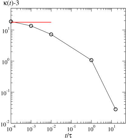
Figure 5: Time evolution for the excess kurtosis in Monte Carlo simulations (circles). The horizontal line represents the theoretical asymptotic behaviour, according to Eq. (11).

Stochastic models are typically constructed assuming specific features for noise terms in the equations. Here we followed a different path, in which the model begets from a genuine microscopic instance endowed with an autonomous dynamics. We have thus been able to provide the first evidence in which the Brownian non-Gaussian diffusion compliant with a stochastic model is independently and exactly produced by a microscopic dynamics. Noting that the anomalous diffusion of the polymer CM is ruled by its equilibrium critical behaviour, and ultimately by the value of the entropic critical exponent $\gamma$, it would be worthwhile to extend future theoretical and numerical considerations to models of polymers either characterized by different, fixed, topologies [56] (i.e. linear vs star or branched polymer ) or to polymeric systems still in diluted condition but undergoing conformational phase transitions such as the Theta- or the adsorption-transition [39, 41]. For instance, one should compare the theoretical predictions of the CM diffusion of linear polymers undergoing a collapse transition from a swollen to a compact phase with gran canonical (i.e $N$-varying ensemble) Monte Carlo simulations of interacting self-avoiding walks on the cubic lattice [41]. Similarly, one might look at the CM diffusion of three-dimensional SAWs once adsorbed on an attractive impenetrable wall [57] or localised in proximity of an interface separating two bulk regions characterized by different solvent conditions [58, 59].

References

References

- [1] Bo Wang, Stephen M Anthony, Sung Chul Bae, and Steve Granick. Anomalous yet brownian. Proceedings of the National Academy of Sciences, 106(36):15160–15164, 2009.
- [2] Bo Wang, James Kuo, Sung Chul Bae, and Steve Granick. When brownian diffusion is not gaussian. Nature materials, 11(6):481, 2012.
- [3] Toshihiro Toyota, David A Head, Christoph F Schmidt, and Daisuke Mizuno. Non-gaussian athermal fluctuations in active gels. Soft Matter, 7(7):3234–3239, 2011.
- [4] Changqian Yu, Juan Guan, Kejia Chen, Sung Chul Bae, and Steve Granick. Single-molecule observation of long jumps in polymer adsorption. ACS Nano, 7(11):9735, 2013.
- [5] Changqian Yu and Steve Granick. Revisiting polymer surface diffusion in the extreme case of strong adsorption. Langmuir, 30:14538, 2014.
- [6] Indrani Chakraborty and Yael Roichman. Disorder-induced fickian, yet non-gaussian diffusion in heterogeneous media. Physical Review Research, 2(2):022020, 2020.
- [7] Eric R Weeks, John C Crocker, Andrew C Levitt, Andrew Schofield, and David A Weitz. Three-dimensional direct imaging of structural relaxation near the colloidal glass transition. Science, 287(5453):627–631, 2000.
- [8] Caroline E Wagner, Bradley S Turner, Michael Rubinstein, Gareth H McKinley, and Katharina Ribbeck. A rheological study of the association and dynamics of muc5ac gels. Biomacromolecules, 18(11):3654–3664, 2017.
- [9] Jae-Hyung Jeon, Matti Javanainen, Hector Martinez-Seara, Ralf Metzler, and Ilpo Vattulainen. Protein crowding in lipid bilayers gives rise to non-gaussian anomalous lateral diffusion of phospholipids and proteins. Physical Review X, 6(2):021006, 2016.
- [10] Eiji Yamamoto, Takuma Akimoto, Antreas C Kalli, Kenji Yasuoka, and Mark SP Sansom. Dynamic interactions between a membrane binding protein and lipids induce fluctuating diffusivity. Science advances, 3(1):e1601871, 2017.
- [11] Stella Stylianidou, Nathan J Kuwada, and Paul A Wiggins. Cytoplasmic dynamics reveals two modes of nucleoid-dependent mobility. Biophysical journal, 107(11):2684–2692, 2014.
- [12] Bradley R Parry, Ivan V Surovtsev, Matthew T Cabeen, Corey S O’Hern, Eric R Dufresne, and Christine Jacobs-Wagner. The bacterial cytoplasm has glass-like properties and is fluidized by metabolic activity. Cell, 156(1-2):183–194, 2014.
- [13] Matthias Christoph Munder, Daniel Midtvedt, Titus Franzmann, Elisabeth Nuske, Oliver Otto, Maik Herbig, Elke Ulbricht, Paul Müller, Anna Taubenberger, Shovamayee Maharana, et al. A ph-driven transition of the cytoplasm from a fluid-to a solid-like state promotes entry into dormancy. elife, 5:e09347, 2016.
- [14] Andrey G Cherstvy, Oliver Nagel, Carsten Beta, and Ralf Metzler. Non-gaussianity, population heterogeneity, and transient superdiffusion in the spreading dynamics of amoeboid cells. Physical Chemistry Chemical Physics, 20(35):23034–23054, 2018.
- [15] Yunyun Li, Fabio Marchesoni, Debajyoti Debnath, and Pulak K Ghosh. Non-gaussian normal diffusion in a fluctuating corrugated channel. Physical Review Research, 1(3):033003, 2019.
- [16] Alejandro Cuetos, Neftalí Morillo, and Alessandro Patti. Fickian yet non-gaussian diffusion is not ubiquitous in soft matter. Physical Review E, 98(4):042129, 2018.
- [17] Simona Hapca, John W Crawford, and Iain M Young. Anomalous diffusion of heterogeneous populations characterized by normal diffusion at the individual level. Journal of the Royal Society Interface, 6(30):111–122, 2008.
- [18] Raffaele Pastore, Antonio Ciarlo, Giuseppe Pesce, Francesco Greco, and Antonio Sasso. Rapid fickian yet non-gaussian diffusion after subdiffusion. Physical Review Letters, 126(15):158003, 2021.
- [19] Raffaele Pastore and Guido Raos. Glassy dynamics of a polymer monolayer on a heterogeneous disordered substrate. Soft Matter, 11:8083, 2015.
- [20] José M Miotto, Simone Pigolotti, Aleksei V Chechkin, and Sándalo Roldán-Vargas. Length scales in brownian yet non-gaussian dynamics. Physical Review X, 11(3):031002, 2021.
- [21] Francesco Rusciano, Raffaele Pastore, and Francesco Greco. Fickian non-gaussian diffusion in glass-forming liquids. Physical Review Letters, 128:168001, 2022.
- [22] Christian Beck and Ezechiel GD Cohen. Superstatistics. Physica A: Statistical mechanics and its applications, 322:267–275, 2003.
- [23] Christian Beck. Superstatistical brownian motion. Progress of Theoretical Physics Supplement, 162:29–36, 2006.
- [24] Mykyta V Chubynsky and Gary W Slater. Diffusing diffusivity: a model for anomalous, yet brownian, diffusion. Physical review letters, 113(9):098302, 2014.
- [25] Aleksei V Chechkin, Flavio Seno, Ralf Metzler, and Igor M Sokolov. Brownian yet non-gaussian diffusion: from superstatistics to subordination of diffusing diffusivities. Physical Review X, 7(2):021002, 2017.
- [26] Rohit Jain and KL Sebastian. Diffusing diffusivity: a new derivation and comparison with simulations. Journal of Chemical Sciences, 129(7):929–937, 2017.
- [27] Neha Tyagi and Binny J Cherayil. Non-gaussian brownian diffusion in dynamically disordered thermal environments. The Journal of Physical Chemistry B, 121(29):7204–7209, 2017.
- [28] Tomoshige Miyaguchi. Elucidating fluctuating diffusivity in center-of-mass motion of polymer models with time-averaged mean-square-displacement tensor. Physical Review E, 96(4):042501, 2017.
- [29] Vittoria Sposini, Aleksei V Chechkin, Flavio Seno, Gianni Pagnini, and Ralf Metzler. Random diffusivity from stochastic equations: comparison of two models for brownian yet non-gaussian diffusion. New Journal of Physics, 20(4):043044, 2018.
- [30] V Sposini, A Chechkin, and R Metzler. First passage statistics for diffusing diffusivity. Journal of Physics A: Mathematical and Theoretical, 52(4):04LT01, 2018.
- [31] E Barkai and S Burov. Packets of diffusing particles exhibit universal exponential tails. Physical Review Letters, 124:060603, 2020.
- [32] W Wang, E Barkai, and S Burov. Packets of diffusing particles exhibit universal exponential tails. Entropy, 22:697, 2020.
- [33] A Pacheco-Pozo and I M Sokolov. Large deviations in continuous-time random walks. Physical Review E, 103:042116, 2021.
- [34] A Pacheco-Pozo and I M Sokolov. Convergence to a gaussian by narrowing of central peak in brownianyet non-gaussian diffusion in disordered environments. Physical Review Letters, 127:120601, 2021.
- [35] F Baldovin, E Orlandini, and F Seno. Polymerization induces non-gaussian diffusion. Frontiers in Physics, 7:124, 2019.
- [36] S Nampoothiri, E Orlandini, F Seno, and F Baldovin. Polymers critical point originates brownian non-gaussian diffusion. Physical Review E, 104:L062501, 2021.
- [37] S Nampoothiri, E Orlandini, F Seno, and F Baldovin. Brownian non-gaussian polymer diffusion and queuing theory in the mean-field limit. New J. Phys., 24:023003, 2022.
- [38] M Hidalgo-Soria and E Barkai. Hitchhiker model for laplace diffusion processes in the cell environment. Physical Review E, 102:012109, 2020.
- [39] P-G de Gennes. Exponents for the excluded volume problem as derived by the wilson method. Physics Letters A, 38:339–340, 1972.
- [40] P-G de Gennes. Scaling Concepts in Polymer Physics. Cornell University Press, 1979.
- [41] C Vanderzande. Lattice Models of Polymers. Cambridge University Press, 1998.
- [42] N Madras and G Slade. The Self-Avoiding Walk. Springer, 2013.
- [43] A. Baumgärtner and K. Binder. Monte carlo studies on the freely jointed polymer chain with excluded volume interaction. J. Chem. Phys., 71:2541, 1979.
- [44] Shyh-Shi Chern, Alfredo E. Cárdenas, and Rob D. Coalson. Three-dimensional dynamic monte carlo simulations of driven polymer transport through a hole in a wall. J. Chem. Phys., 115:7772, 2001.
- [45] N. J. Burroughs and D. Marenduzzo. Nonequilibrium-driven motion in actin networks: Comet tails and moving beads. Phys. Rev. Lett., 98:238302, 2007.
- [46] N Clisby. Calculation of the connective constant for self-avoiding walks via the pivot algorithm. Journal of Physics A: Mathematical and Theoretical, 46(24):245001, 2013.
- [47] N Clisby. Scale-free monte carlo method for calculating the critical exponent of self-avoiding walks. Journal of Physics A: Mathematical and Theoretical, 50:264003, 2017.
- [48] M Doi and Edwards S F. The Theory of Polymer Dynamics. Oxford University Press, 1992.
- [49] W Feller. An Introduction to Probability Theory and Its Applications. John Wiley & Sons, 1968.
- [50] Salomon Bochner. Harmonic analysis and the theory of probability. University of California press, 2020.
- [51] A Berretti and A D Sokal. New monte carlo method for the self-avoiding walk. Journal of Statistical Physics, 40:483, 1985.
- [52] A D Sokal. Monte carlo methods for the self avoiding walk. Nuc.Phys. B - Proceeding Supplements, 47:172–179, 1996.
- [53] N Clisby, R Liang, and G Slade. Self-avoiding walk enumeration via the lace expansion. Journal of Physics A: Mathematical and Theoretical, 40:10973, 2007.
- [54] D Schram, G T Barkema, and R H Bisseling. Exact enumeration of self-avoiding walks. J. Stat. Mech., page P06019, 2011.
- [55] Daniel T Gillespie. Exact stochastic simulation of coupled chemical reactions. Journal of Physical Chemistry, 81:2340–2361, 1977.
- [56] B Duplantier. Statistical mechanics of polymer networks of any topology. Journal of Statistical Physics, 54(3/4):581, 1989.
- [57] EJ Janse Van Rensburg. The statistical mechanics of interacting walks, polygons, animals and vesicles. Oxford Lecture Mathematics and, 2015.
- [58] Ludwik Leibler. Theory of phase equilibria in mixtures of copolymers and homopolymers. 2. interfaces near the consolute point. Macromolecules, 15(5):1283–1290, 1982.
- [59] Maria Serena Causo and Stuart G Whittington. A monte carlo investigation of the localization transition in random copolymers at an interface. Journal of Physics A: Mathematical and General, 36(13):L189, 2003.