Muon capture on deuteron using local chiral potentials

Abstract

The muon capture reaction $\mu^{-}+d\rightarrow n+n+\nu_{\mu}$ in the doublet hyperfine state is studied using nuclear potentials and consistent currents derived in chiral effective field theory, which are local and expressed in coordinate-space (the so-called Norfolk models). Only the largest contribution due to the ${}^{1}S_{0}$ $nn$ scattering state is considered. Particular attention is given to the estimate of the theoretical uncertainty, for which four sources have been identified: (i) the model dependence, (ii) the chiral order convergence for the weak nuclear current, (iii) the uncertainty in the single-nucleon axial form factor, and (iv) the numerical technique adopted to solve the bound and scattering $A=2$ systems. This last source of uncertainty has turned out essentially negligible. The ${}^{1}S_{0}$ doublet muon capture rate $\Gamma^{D}(^{1}S_{0})$ has been found to be $\Gamma^{D}(^{1}S_{0})=255.8(0.6)(4.4)(2.9)$ s^-1, where the three errors come from the first three sources of uncertainty. The value for $\Gamma^{D}(^{1}S_{0})$ obtained within this local chiral framework is compared with previous calculations and found in very good agreement.

I Introduction

The muon capture on deuteron, i.e. the process

$$\mu^{-}+d\rightarrow n+n+\nu_{\mu}\ ,$$ (1)

is one of the few weak nuclear reactions involving light nuclei which, on one side, are experimentally accessible, and, on the other, can be studied using ab-initio methods. Furthermore, it is a process closely linked to the proton-proton weak capture, the so-called $pp$ reaction,

$$p+p\rightarrow d+e^{+}+\nu_{e}\ ,$$ (2)

which, although being of paramount importance in astrophysics, is not experimentally accessible, due to its extremely low rate, and can only be calculated. Since the theoretical inputs to study reaction (2) and reaction (1) are essentially the same, the comparison between experiment and theory for muon capture provides a strong test for the $pp$ studies.

The muon capture reaction (1) can take place in two different hyperfine states, $f=1/2$ and $3/2$. Since it is well known that the doublet capture rate is about 40 times larger than the quartet one (see for instance Ref. Measday (2001)), we will consider the $f=1/2$ state only, and we will focus on the doublet capture rate, $\Gamma^{D}$.

The experimental situation for $\Gamma^{D}$ is quite confused, with available measurements which are relatively old. These are the ones of Refs. Wang et al. (1965); Bertin et al. (1973); Bardin et al. (1986); Cargnelli M, et al. (1989), $365(96)\;\rm{s}^{-1}$, $445(60)\;\rm{s}^{-1}$, $470(29)\;\rm{s}^{-1}$ and $409(40)\;\rm{s}^{-1}$, respectively. All these data are consistent with each other within the experimental uncertainties, which are however quite large. In order to clarify the situation, an experiment with the aim of measuring $\Gamma^{D}$ with a 1% accuracy is currently performed at the Paul Scherrer Institute, in Switzerland, by the MuSun Collaboration Kammel (2013).

Many theoretical studies are available for the muon capture rate $\Gamma^{D}$. A review of the available literature of up to about ten years ago can be found in Ref. Marcucci (2012). Here we focus on the work done in the past ten years. To the best of our knowledge, the capture rate $\Gamma^{D}$ has been studied in Refs. Adam et al. (2012); Marcucci et al. (2011, 2012); Golak et al. (2014); Acharya et al. (2018). The studies of Refs. Marcucci et al. (2011); Golak et al. (2014) have been performed within the phenomenological approach, using phenomenological potentials and currents. In Ref. Marcucci et al. (2011), the first attempt to use chiral effective field theory ($\chi$EFT) was presented, within the so-called hybrid approach, where a phenomenological nuclear interaction is used in conjunction with $\chi$EFT weak nuclear charge and current operators. In the study we present in this contribution, though, we are interested not only in the determination of $\Gamma^{D}$, but also in an assessment of the theoretical uncertainty. This can be grasped more comfortably and robustly within a consistent $\chi$EFT approach. Therefore, we review only the theoretical works of Refs. Adam et al. (2012); Marcucci et al. (2012); Acharya et al. (2018), which have been performed within a consistent $\chi$EFT. The studies of Refs. Adam et al. (2012) and Marcucci et al. (2012) were essentially performed in parallel. They both employed the latest (at those times) nuclear chiral potentials and consistent weak current operators. In Ref. Adam et al. (2012), the doublet capture rate was found to be $\Gamma^{D}=388.1(4.3)$ s^-1, when the $NN$ chiral potentials of Ref. Entem and Machleidt (2003), obtained up to next-to-next-to-next-to leading order (N3LO) in the chiral expansion, were used. When only the ${}^{1}S_{0}$ channel of the final $nn$ scattering state was retained, it was found $\Gamma^{D}(^{1}S_{0})=247.7(2.8)$ s^-1. In Ref. Marcucci et al. (2012), a simultaneous study of the muon capture on deuteron and ³He was perfomed using the same N3LO chiral potentials, but varying the potential cutoff $\Lambda=500,600$ MeV Entem and Machleidt (2003); Machleidt and Entem (2011), and consequently refitting consistently for each value of $\Lambda$ the low-energy constants (LECs) entering into the axial and vector current operators. For the muon capture on deuteron, it was obtained $\Gamma^{D}=399(3)$ s^-1, the spread accounting for the cutoff sensitivity, as well as uncertainties in the LECs and electroweak radiative corrections. When only the ${}^{1}S_{0}$ channel is considered, $\Gamma^{D}(^{1}S_{0})=254.9(1.4)$ s^-1, where, in this case, the (small) uncertainty arising from electroweak radiative corrections is not included. In the case of the muon capture on ³He, an excellent agreement with the available extremely accurate experimental datum was found. Although obtained by different groups and with some differences in the axial and vector current operators adopted in the calculations, the results of Refs. Adam et al. (2012) and Marcucci et al. (2012) for $\Gamma^{D}$ and $\Gamma^{D}(^{1}S_{0})$ should be considered in reasonable agreement. It should be mentioned that in both studies of Refs. Adam et al. (2012) and Marcucci et al. (2012), a relation between the LEC entering the axial current operator (denoted with $d_{R}$) and $c_{D}$, one of the two LECs entering the three-nucleon potential (the other one being $c_{E}$) was taken from Ref. Gazit et al. (2009). Then, the $A=3$ binding energies and the Gamow-Teller of the triton $\beta$-decay were used to fix both $c_{D}$ (and consequently $d_{R}$) and $c_{E}$ for each given potential and cutoff $\Lambda$. Unfortunately, the relation between $d_{R}$ and $c_{D}$ of Ref. Gazit et al. (2009) has been found to be missing of a factor $-1/4$, as clearly stated in the Erratum of Ref. Marcucci et al. (2012) (see also the Erratum of Ref. Gazit et al. (2009)). While the work of Ref. Adam et al. (2012) has not yet been revisited, that of Ref. Marcucci et al. (2012) has been corrected, finding very small changes in the final results, which become $\Gamma^{D}=398(3)$ s^-1 and $\Gamma^{D}(^{1}S_{0})=253.5(1.2)$ s^-1.

The most recent and systematic study of reaction (1) in $\chi$EFT, even if only retaining the ${}^{1}S_{0}$ $nn$ channel, is that of Ref. Acharya et al. (2018). There, $\Gamma^{D}(^{1}S_{0})$ has been calculated using a pool of 42 non-local chiral potentials up to next-to-next-to-leading order (N2LO), with a regulator cutoff $\Lambda$ in the range 450-600 MeV and six different energy ranges in the $NN$ scattering database Carlsson et al. (2016). The consistent axial and vector currents were constructed (with the correct relation between $d_{R}$ and $c_{D}$), and a simultaneous fitting procedure for all the involved LECs was adopted. The final result was found to be $\Gamma^{D}(^{1}S_{0})=252.8(4.6)(3.9)\;\rm{s}^{-1}$, in excellent agreement with Ref. Marcucci et al. (2012). Here the first error is due to the truncation in the chiral expansion and the second one to the uncertainty in the parameterization of the single-nucleon axial form factor (see below). In Ref. Acharya et al. (2018) it was also questioned the accuracy of the variational method used to calculate the deuteron and $nn$ scattering wave functions in Refs. Marcucci et al. (2011, 2012). This same issue was already raised in Ref. Acharya et al. (2017), where it was found that a non-proper treatment of the infrared cutoff when the bound-state wave function is represented in a truncated basis (as in the case of Refs. Marcucci et al. (2011, 2012)) can lead to an error of the order of $\sim 1$% in the few-nucleon capture cross sections and astrophysical $S$-factors (as for instance that of the $pp$ reaction).

The chiral nuclear potentials involved in all the above mentioned studies are highly non-local, and are expressed in momentum-space. This is clearly less desirable compared with $r$-space in the case of the $pp$ reaction, where the treatment in momentum-space of the Coulomb interaction and of the higher-order electromagnetic effects is rather cumbersome. In order to overcome these difficulties, local chiral potentials expressed in $r$-space would be highly desirable. These have been developed only in recent years, as discussed in the recent review of Ref. Piarulli and Tews (2020). These potentials are very accurate, and have proven to be extremely successful in order to describe the structure and dynamics of light and medium-mass nuclei. In particular, we are interested in this work to the models of Ref. Piarulli et al. (2016), the so-called Norfolk potentials, for which, in these years, consistent electromagnetic and weak transition operators have been constructed Baroni et al. (2018); Schiavilla et al. (2019); Gnech and Schiavilla (2022). This local chiral framework has been used to calculate energies Piarulli et al. (2018), charge radii Gandolfi et al. (2020) and various electromagnetic observables in light nuclei, as the charge form factors in $A=6,12$ Gandolfi et al. (2020) and the magnetic structure of few-nucleon systems Gnech and Schiavilla (2022). It has been used also to study weak transitions in light nuclei King et al. (2020a, b), the muon captures on $A=3,6$ nuclei King et al. (2022a), neutrinoless double $\beta$-decay for $A=6,12$  Cirigliano et al. (2019) and the $\beta$-decay spectra in $A=6$ King et al. (2022b), and, finally, also the equation of state of pure neutron matter Piarulli et al. (2020); Lovato et al. (2022). However, the use of the Norfolk potentials to study the muon capture on deuteron (1) and the $pp$ reaction (2) is still lacking. It is one of the aim of the present work to start this path. Given the fact that $\Gamma^{D}(^{1}S_{0})$ is the main contribution to $\Gamma^{D}$, and the ${}^{1}S_{0}$ channel is also the only one of interest for the $pp$ fusion Acharya et al. (2019); Marcucci et al. (2013), we focus here our attention only on $\Gamma^{D}(^{1}S_{0})$. A full calculation of $\Gamma^{D}$, together with the rates for muon capture on $A=3$ and 6 nuclei, is currently underway. The second aim of the present study is to provide a more robust determination of the theoretical uncertainty compared with the work of Ref. Marcucci et al. (2012), although probably not as robust as the full work presented in Ref. Acharya et al. (2018). However, the procedure we plan to apply in the present work is much simpler and, as it will be shown below, with a quite similar final outcome. In fact, we will consider four sources of uncertainties: (i) the first one is due to model dependence. In this study, the use of the local Norfolk potentials will allow us to take into consideration the uncertainty arising from the cutoff variation, as well as the energy ranges in the $NN$ scattering database up to which the LECs are fitted. In fact, as it will be explained in Sec. II.2, we will employ four different versions of the Norfolk potentials, obtained using two different sets of short- and long-range cutoffs, and two different energy ranges, up to 125 MeV or up to 200 MeV, in the $NN$ scattering database. (ii) A second source of uncertainty arises from the chiral order convergence. In principle, this should be investigated by maintaining the same order for potentials and weak nuclear currents. However, at present, the Norfolk potentials, for which weak current operators have been consistently constructed, are those obtained at N3LO. As a matter of fact, this chiral order is needed to reach a good accuracy in the description of the $NN$ systems and of light nuclei. Therefore, it is questionable whether a study of reaction (1) using potentials and currents at a chiral order which do not even reproduce the nuclear systems under consideration, would be of real interest. As a consequence, we will study in the present work only the chiral order convergence for the weak nuclear currents, keeping fixed the chiral order of the adopted potentials. (iii) A third source of uncertainty is due to the uncertainty in the parameterization of single-nucleon axial form factor $g_{A}(q_{\sigma}^{2})$ as function of the squared four-momentum transfer $q_{\sigma}^{2}$. This aspect will be discussed in details in Sec. II.2. Here we only notice that the most recent parameterization for the single-nucleon axial form factor is given by

$$g_{A}(q_{\sigma}^{2})=g_{A}\left(1-\frac{1}{6}r_{A}^{2}q_{\sigma}^{2}+...\right)\ ,$$ (3)

where the dots indicate higher-order terms, which are typically disregarded, and $r_{A}$ is the axial charge radius, its square being given by $r_{A}^{2}=0.46(16)$ fm² Hill et al. (2018). The large uncertainty on $r_{A}^{2}$ will affect significantly the total uncertainty budget, as already found in Ref. Acharya et al. (2018). (iv) A final source of uncertainty is the one arising from the numerical technique adopted to solve the bound and scattering $A=2$ systems. In fact, taking into consideration the arguments of Ref. Acharya et al. (2017), we have decided to use two methods. The first one is the method already developed in Refs. Marcucci et al. (2011, 2012), i.e. a variational method, in which the bound and scattering wave functions are expanded on a known basis, and the unknown coefficients of these expansions are obtained by means of variational principles. The second method is the so-called Numerov method, where the tail of the bound state wave function is in fact imposed “by hand” (see Sec. (II.3)). This last source of uncertainty will be shown to be completely negligible. This seems to be in contrast, at least for the observable here under study, with the conclusions of Ref. Acharya et al. (2017).

The paper is organized as follows: in Sec. II we will present the theoretical formalism, providing a schematic derivation for $\Gamma^{D}(^{1}S_{0})$ in Sec. II.1, a description of the adopted nuclear potentials and currents in Sec. II.2, and a discussion of the methods used to calculate the deuteron and $nn$ wave functions in Sec. II.3. The results for $\Gamma^{D}(^{1}S_{0})$ will be presented and discussed in Sec. III, and some concluding remarks and an outlook will be given in Sec. IV.

II Theoretical formalism

We discuss in this section the theoretical formalism developed to calculate the muon capture rate. In particular, in Sec. II.1 we report the main steps of the formalism used to derive the differential and the total muon capture rate on deuteron in the initial doublet hyperfine state. A thourough discussion has been given in Ref. Marcucci et al. (2011). In Sec. II.2 we report the main characteristics of the nuclear potentials and currents we have used in the present study. Finally in Sec. II.3 we discuss the variational and the Numerov methods used to calculate the deuteron bound and $nn$ scattering wave functions.

II.1 Observables

The differential capture rate in the doublet initial hyperfine state ${d\Gamma^{D}}/{dp}$ can be written as Marcucci et al. (2011)

$$\frac{d\Gamma^{D}}{dp}=E_{\nu}^{2}\,\left[1-{E_{\nu}\over(m_{\mu}+m_{d})}\right]\,\frac{p^{2}d{\hat{\bf p}}}{8\pi^{4}}\,\overline{|T_{W}|^{2}}\ ,$$ (4)

where ${\bf p}$ is the $nn$ relative momentum, and

$$E_{\nu}=\frac{(m_{\mu}+m_{d})^{2}-4m_{n}^{2}-4p^{2}}{2(m_{\mu}+m_{d})}\ ,$$ (5)

with $m_{\mu}$, $m_{n}$, and $m_{d}$ being the muon, neutron, and deuteron masses. The transition amplitude $\overline{|T_{W}|^{2}}$ reads Marcucci et al. (2011)

$$\overline{|T_{W}|^{2}}=\frac{1}{2f+1}\sum_{s_{1}s_{2}h_{\nu}}\sum_{f_{z}}|T_{W}(f,f_{z};s_{1},s_{2},h_{\nu})|^{2}\ ,$$ (6)

where $f,f_{z}$ indicate the initial hyperfine state, fixed here to be $f=1/2$, while $s_{1}$, $s_{2}$, and $h_{\nu}$ denote the spin $z$-projection for the two neutrons and the neutrino helicity state. In turn, $T_{W}(f,f_{z};s_{1},s_{2},h_{\nu})$ is given by

$$T_{W}(f,f_{z};s_{1},s_{2},h_{\nu}) \equiv \langle nn,s_{1},s_{2};\nu,h_{\nu}\,|\,H_{W}\,|\,(\mu,d);f,f_{z}\rangle$$ (7)

$$\simeq {G_{V}\over\sqrt{2}}\psi_{1s}^{\rm av}\sum_{s_{\mu}s_{d}}\langle{1\over 2}s_{\mu},1s_{d}|ff_{z}\rangle\,l_{\sigma}(h_{\nu},\,s_{\mu})\,\langle\Psi_{{\bf p},s_{1}s_{2}}(nn)|j^{\sigma}({\bf q})|\Psi_{d}(s_{d})\rangle\ ,$$

with $l_{\sigma}$ and $j^{\sigma}$ being the leptonic and hadronic current densities, respectively Marcucci et al. (2011), written as

$$l_{\sigma}(h_{\nu},\,s_{\mu})\equiv{\overline{u}}({\bf k}_{\nu},h_{\nu})\,\gamma_{\sigma}\,(1-\gamma_{5})u({\bf k}_{\mu},s_{\mu})\>\>\>,$$ (8)

and

$$j^{\sigma}({\bf q})=\int{\rm d}{\bf x}\,{\rm e}^{{\rm i}{\bf q}\cdot{\bf x}}\,j^{\sigma}({\bf x})\equiv(\rho({\bf q}),{\bf j}({\bf q}))\>\>\>.$$ (9)

Here the leptonic momentum transfer ${\bf q}$ is defined as ${\bf q}={\bf k}_{\mu}-{\bf k}_{\nu}\simeq-{\bf k}_{\nu}$. Furthermore, $\Psi_{d}(s_{d})$ and $\Psi_{{\bf p},s_{1}s_{2}}(nn)$ are the initial deuteron and final $nn$ wave functions, respectively, with $s_{d}$ indicating the deuteron spin $z$-projection. Finally, in Eq. (7), the function $\psi_{1s}^{\rm av}$ represents the $1s$ solution of the Schrödinger equation for the initial muonic $\mu-d$ atom. Since the muon is essentially at rest, it can be approximated as Marcucci et al. (2011); Walecka (1995)

$$|\psi_{1s}^{\rm av}|\equiv\,|\psi_{1s}(0)|\,=\,\sqrt{{(\alpha\,\mu_{\mu d})^{3}\over\pi}}\ ,$$ (10)

where $\psi_{1s}(0)$ denotes the Bohr wave function for a point charge $e$ evaluated at the origin, $\mu_{\mu d}$ is the reduced mass of the $(\mu,d)$ system, and $\alpha=1/137.036$ is the fine-structure constant.

The final $nn$ wave fucntion can be expanded in partial waves as

$$\Psi_{{\bf p},s_{1}s_{2}}(nn)=4\pi\sum_{S}\langle\frac{1}{2}s_{1},\frac{1}{2}s_{2}|SS_{z}\rangle\sum_{LL_{z}JJ_{z}}{\rm i}^{L}Y^{*}_{LL_{z}}({\hat{\bf p}})\langle SS_{z},LL_{z}|JJ_{z}\rangle\,\overline{\Psi}_{nn}^{LSJJ_{z}}(p)\>\>,$$ (11)

where $\overline{\Psi}_{nn}^{LSJJ_{z}}(p)$ is the $nn$ wave function with orbital angular momentum $LL_{z}$, total spin $SS_{z}$, and total angular momentum $JJ_{z}$. In the present work, we restrict our study to the $L=0$ state (${}^{1}S_{0}$ in spectroscopic notation).

Using standard techniques as described in Refs. Marcucci et al. (2011); Walecka (1995), a multipole expansion of the weak charge, $\rho({\bf q})$, and current, ${\bf j}({\bf q})$, operators can be performed, resulting in

$$\langle\overline{\Psi}_{nn}^{LSJJ_{z}}(p)|\rho({\bf q})|\Psi_{d}(s_{d})\rangle = \sqrt{4\pi}\sum_{\Lambda\geq 0}\sqrt{2\Lambda+1}\,\,{\rm i}^{\Lambda}\frac{\langle 1s_{d},\Lambda 0|JJ_{z}\rangle}{\sqrt{2J+1}}C_{\Lambda}^{LSJ}(q)\ ,$$ (12)

$$\langle\overline{\Psi}_{nn}^{LSJJ_{z}}(p)|j_{z}({\bf q})|\Psi_{d}(s_{d})\rangle = -\sqrt{4\pi}\sum_{\Lambda\geq 0}\sqrt{2\Lambda+1}\,\,{\rm i}^{\Lambda}\frac{\langle 1s_{d},\Lambda 0|JJ_{z}\rangle}{\sqrt{2J+1}}L_{\Lambda}^{LSJ}(q)\ ,$$ (13)

$$\langle\overline{\Psi}_{nn}^{LSJJ_{z}}(p)|j_{\lambda}({\bf q})|\Psi_{d}(s_{d})\rangle = \sqrt{2\pi}\sum_{\Lambda\geq 1}\sqrt{2\Lambda+1}\,\,{\rm i}^{\Lambda}\frac{\langle 1s_{d},\Lambda-\lambda|JJ_{z}\rangle}{\sqrt{2J+1}}$$ (14)

$$\times [-\lambda M_{\lambda}^{LSJ}(q)+E_{\Lambda}^{LSJ}(q)]\ ,$$

where $\lambda=\pm 1$, and $C_{\Lambda}^{LSJ}(q)$, $L_{\Lambda}^{LSJ}(q)$, $E_{\Lambda}^{LSJ}(q)$ and $M_{\Lambda}^{LSJ}(q)$ denote the reduced matrix elements (RMEs) of the Coulomb ($C$), longitudinal ($L$), transverse electric ($E$) and transverse magnetic ($M$) multipole operators, as defined in Ref. Marcucci et al. (2011). Since the weak charge and current operators have scalar/polar-vector $(V)$ and pseudo-scalar/axial-vector $(A)$ components, each multipole consists of the sum of $V$ and $A$ terms, having opposite parity under space inversions. Given that in this study only the ${}^{1}S_{0}$ contribution is considered, the only contributing multipoles are $C_{1}(A)$, $L_{1}(A)$, $E_{1}(A)$, $M_{1}(V)$, where the superscripts $LSJ$ have been dropped.

In order to calculate the differential capture rate $d\Gamma^{D}/dp$ in Eq. (4), we need to integrate over ${\hat{\bf p}}$. This is done numerically using Gauss-Legendre of the order of 10, so that an accuracy to better than 1 part in $10^{3}$ can be achieved. Finally, the total capture rate $\Gamma^{D}$ is obtained as

$$\Gamma^{D}=\int_{0}^{p_{max}}\frac{d\Gamma^{D}}{dp}dp\ ,$$ (15)

where $p_{max}$ is the maximum value of the momentum $p$. In order to find the smallest needed number of grid points to reach convergence, we have computed the capture rate by integrating over several grids starting from a minimum value of 20 points up to a maximum of 80. We have verified that the results obtained integrating over 20 or 40 points differ of about 0.1 s^-1, while the ones obtained with 40, 60 and 80 points differ by less than 0.01 s^-1. Therefore, we have used 60 grid points in all the studied cases mentioned below.

II.2 Nuclear potentials and currents

In this study we consider four different nuclear interaction models, and consistent weak current operators, derived in $\chi$EFT. We decided to concentrate our attention on the recent local $r$-space potentials of Ref. Piarulli et al. (2016) (see also Ref. Piarulli and Tews (2020) for a recent review). The motivation behind this choice is mostly related to the fact that in the future we plan to use this same formalism to the $pp$ reaction, for which the Coulomb interaction, and also electromagnetic higher order contributions, play a significant role at the accuracy level reached by theory. The possibility to work in $r$-space is clearly an advantage compared with momentum-space, which would be the unavoidable choice when using non-local potentials. However, in momentum-space the full electromagnetic interaction between the two protons is not easy to be taken into account. The potentials of Ref. Piarulli et al. (2016), which we will refer to as Norfolk potentials (denoted as NV), are chiral interactions that include, beyond pions and nucleons, also $\Delta$-isobar degrees of freedom explicitly. The short-range (contact) part of the interaction receives contributions at leading order (LO), next-to-leading order (NLO) and next-to-next-to-next-to-leading order (N3LO), while the long-range components arise from one- and two-pion exchanges, and are retained up to next-to-next-to-leading order (N2LO). By truncating the expansion at N3LO, there are 26 LECs which have been fitted to the $NN$ Granada database Navarro Pérez et al. (2013, 2014a, 2014b), obtaining two classes of Norfolk potentials, depending on the range of laboratory energies over which the fits have been carried out: the NVI potentials have been fitted in the range 0–125 MeV, while for the NVII potentials the range has been extended up to 200 MeV. For each class of potential, two cutoff functions $C_{R_{S}}(r)$ and $C_{R_{L}}(r)$ have been used to regularize the short- and long-range components, respectively. These functions have been defined as

$$C_{R_{S}}(r) = \frac{1}{\pi^{\frac{3}{2}}R_{S}^{3}}{\rm e}^{-(r/R_{S})^{2}}\ ,$$ (16)

$$C_{R_{L}}(r) = 1-\frac{1}{(r/R_{L})^{6}{\rm e}^{(r-R_{L})/a_{L}}+1}\ ,$$ (17)

with $a_{L}\equiv R_{L}/2$. Two different sets of cutoff values have been considered, $(R_{S};R_{L})=(0.7;1.0)$ and $(0.8;1.2)$, and the resulting models have been labelled “a” and “b”, respectively. All these potentials are very accurate: in fact, the $\chi^{2}$/datum for the NVIa, NVIIa, NVIb, and NVIIb potentials are, respectively, 1.05, 1.37, 1.07, and 1.37 Piarulli et al. (2016).

We turn now our attention to the weak transition operators. When only the ${}^{1}S_{0}$ $nn$ partial wave is included, we have seen that the contributing multipoles are $C_{1}(A)$, $L_{1}(A)$, $E_{1}(A)$ and $M_{1}(V)$. Consequently, the weak vector charge operator is of no interest in the process under consideration, and we will not discuss it here. The weak vector current entering $M_{1}(V)$ can be obtained from the isovector electromagnetic current, performing a rotation in the isospin space, i.e. with the substitutions

$$\tau_{i,z} \Rightarrow \tau_{i,\pm}=(\tau_{i,x}\pm i\tau_{i,y})/2\ ,$$ (18)

$$({\bm{\tau}}_{i}\times{\bm{\tau}}_{j})_{z} \Rightarrow ({\bm{\tau}}_{i}\times{\bm{\tau}}_{j})_{\pm}=({\bm{\tau}}_{i}\times{\bm{\tau}}_{j})_{x}\pm i({\bm{\tau}}_{i}\times{\bm{\tau}}_{j})_{y}\ .$$ (19)

Therefore, we will review the various contributions to the electromagnetic current, even if, in fact, we are interest only to their isovector components. The electromagnetic current operators up to one loop have been most recently reviewed in Ref. Gnech and Schiavilla (2022). Here we only give a synthetic summary. Following the notation of Ref. Gnech and Schiavilla (2022), we denote with $Q$ the generic low-momentum scale. The LO contribution, at order $Q^{-2}$, consists of the single-nucleon current, while at the NLO, or at order $Q^{-1}$, there is the one-pion-exchange (OPE) contribution. The relativistic correction to the LO single-nucleon current provides the first contribution of order $Q^{0}$ (N2LO). Furthermore, since the Norfolk interaction models retain explicitly $\Delta$-isobar degrees of freedom, we take into account also the N2LO currents originating from explicit $\Delta$ intermediate states. Finally, the currents at order $Q^{1}$ (N3LO) consist of (i) terms generated by minimal substitution in the four-nucleon contact interactions involving two gradients of the nucleon fields and by non-minimal couplings to the electromagnetic field; (ii) OPE terms induced by $\gamma\pi N$ interactions of sub-leading order; and (iii) one-loop two-pion-exchange terms. A thourough discussion of all these contribuions as well as their explicit expressions can be found in Ref. Gnech and Schiavilla (2022). Here we only remark that (i) the various contributions are derived in momentum space and have power law behavior at large momenta, or short range. Therefore, they need to be regularized. The procedure adopted here, as in Ref. Gnech and Schiavilla (2022), is to carry out first the Fourier transforms of the various terms. This results in $r$-space operators which are highly singular at vanishing inter-nucleon separations. Then the singular behavior is removed by multiplying the various terms by appropriate $r$-space cutoff functions, identical to those of the Norfolk potentials of Ref. Piarulli et al. (2016). More details can be found in Refs. Schiavilla et al. (2019); Gnech and Schiavilla (2022). (ii) There are 5 LECs in the electromagnetic currents which do not enter in the nuclear potentials and need to be fitted using electromagnetic observables. These LECs enter the current operators at N3LO, in particular two of them are present in the currents arising from non-minimal couplings to the electromagnetic field, and three of them are present in the sub-leading isoscalar and isovector OPE contributions. In this study, these LECs are determined by a simultaneous fit to the $A=2–3$ nuclei magnetic moments and to the deuteron threshold electrodisintegration at backward angles over a wide range of momentum transfers Gnech and Schiavilla (2022). In this work we used the LECs labelled with set A in Ref. Gnech and Schiavilla (2022).

The axial current operators used in the present work are the ones of Ref. Baroni et al. (2018). They include the LO term, of order $Q^{-3}$, which arises from the single-nucleon axial current, and the N2LO and N3LO terms (scaling as $Q^{-1}$ and $Q^{0}$, respectively), consisting of the relativistic corrections and $\Delta$ contributions at N2LO, and of OPE and contact-terms at N3LO. Note that at NLO, here of order $Q^{-2}$, there is no contribution in $\chi$EFT. The explicit $r$-space expression of these operators can be found in Ref. Baroni et al. (2018). Here we only remark that all contributions have been regularized at short and long range consistently with the regulator functions used in the Norfolk potentials. Furthermore, the N3LO contact-term presents a LEC, here denoted with $z_{0}$ (but essentially equal to the $d_{R}$ LEC mentioned in Sec. I), defined as

$$z_{0}=\frac{g_{A}}{2}\frac{m_{\pi}^{2}}{f_{\pi}^{2}}\frac{1}{(m_{\pi}R_{S})^{3}}\left[-\frac{m_{\pi}}{4g_{A}\Lambda_{\chi}}c_{D}+\frac{m_{\pi}}{3}\left(c_{3}+2c_{4}\right)+\frac{m_{\pi}}{6m}\right]\ .$$ (20)

Here $g_{A}=1.2723(23)$ is the single-nucleon axial coupling constant, $m=938.9$ MeV the nucleon mass, $m_{\pi}=138.04$ MeV and $f_{\pi}=97.4$ MeV the pion mass and decay constant, $\Lambda_{\chi}\sim 1$ GeV the chiral-symmetry breaking scale, and $c_{3}=-0.79$ and $c_{4}=1.33$ two LECs entering the $\pi\pi N$ Lagrangian at N2LO and taken from the fit of the pion-nucleon scattering data with $\Delta$-isobar as explicit degrees of freedom Krebs et al. (2007). As mentioned above, $c_{D}$ is one of the two LECs which enter the three-nucleon interaction, the other being denoted with $c_{E}$. The two LECs $c_{D}$ (and consequently $z_{0}$) and $c_{E}$ have been fitted to simultaneously reproduce the experimental trinucleon binding energies and the central value of the Gamow-Teller matrix element in triton $\beta$-decay. The explicit values for $c_{D}$ are $-0.635$, $-4.71$, $-0.61$ and $-5.25$ for the NVIa, NVIb, NVIIa, and NVIIb potentials respectively.

The nuclear axial charge has a much simpler structure compared to the axial and vector currents, and we have used the operators as derived in Ref. Baroni et al. (2016). At LO, i.e. at order $Q^{-2}$, it retains the one-body term, which gives the most important contribution. At NLO (order $Q^{-1}$) the OPE contribution appears, which however has been found almost negligible in this study. The N2LO contributions (order $Q^{0}$) exactly vanish, and at N3LO (order $Q^{1}$) there are two-pion exchange terms and new contact terms where new LECs appear. The N3LO has not been included in the calculation, since the new LECs have not been fixed yet. However, we have found the contribution of $C_{1}(A)$ to be two orders of magnitude smaller compared to the one from the other multipoles. Therefore, the effect of the axial current correction at N3LO can be safely disregarded.

All the axial charge and current contributions are multiplied by the single-nucleon axial coupling constant, $g_{A}(q_{\sigma}^{2})$, written as function of the squared of the four-momentum transfer $q_{\sigma}^{2}$. Contrary to the triton $\beta$-decay, in the case of the muon capture on deuteron, the four-momentum transfer is quite large. The dependence of $g_{A}(q_{\sigma}^{2})$ on $q_{\sigma}^{2}$ is therefore crucial and, as already mentioned in Sec. I, it is a source of theoretical uncertainty in this study. In the past, it has been used for $g_{A}(q_{\sigma}^{2})$ a dipole form Marcucci et al. (2011), but in Ref. Meyer et al. (2016) it has been argued that the dipole form introduces an uncontrolled systematic error in estimating the value of the axial form factor. Alternatively, it has been proposed to use the small-momenta expansion, which leads to the expression of Eq. (3). We have decided to use in our study the new parameterization for $g_{A}(q_{\sigma}^{2})$ of Eq. (3), but with a slightly smaller uncertainty on the the axial charge radius $r_{A}$ compared with Ref. Meyer et al. (2016), as discussed in Ref. Hill et al. (2018). In this work, $r_{A}$ has been chosen as the weighted average of the values obtained by two independent procedures having approximately the same accuracy, about $50\%$. One procedure is the one of Ref. Meyer et al. (2016), and uses for the axial form factor a convergent expansion given by

$$g_{A}(q_{\sigma}^{2})=\sum_{k=0}^{k_{max}}a_{k}z(q_{\sigma}^{2})^{k}\ ,$$ (21)

where the variable $z(q_{\sigma}^{2})$ is defined as

$$z(q_{\sigma}^{2})=\frac{\sqrt{t_{cut}-q_{\sigma}^{2}}-\sqrt{t_{cut}-t_{0}}}{\sqrt{t_{cut}-q_{\sigma}^{2}}+\sqrt{t_{cut}-t_{0}}}\ ,$$ (22)

with $t_{cut}=9\;m_{\pi}^{2}$ and $-\infty<t_{0}<t_{cut}$. In Eq. (21), $a_{k}$ are the expansion parameters which encode the nuclear structure information and need to be experimentally fixed. From $g_{A}(q_{\sigma}^{2})$ in Eq. (21), we can obtain $r_{A}^{2}$ as Meyer et al. (2016)

$$\frac{1}{6}r_{A}^{2}\equiv\frac{1}{g_{A}(0)}\left.\frac{dg_{A}(q_{\sigma}^{2})}{dq_{\sigma}^{2}}\right|_{q_{\sigma}^{2}=0}\ .$$ (23)

The value for $r^{2}_{A}$ is obtained fitting experimental data of neutrino scattering on deuterium and it is found to be $r^{2}_{A}\left(z\right.$ exp.$\left.\nu\right)=0.46(22)$ fm² Meyer et al. (2016).

Alternatively it is possible to obtain $r^{2}_{A}$ from experiments on muonic capture on proton, as done by the MuCap Collaboration. To date these experiments are characterized by an overall accuracy of 1%, but a future experiment plans to reduce this uncertainty to about 0.33% Hill et al. (2018). In this case, $r^{2}_{A}\left(\right.$MuCap$\left.\right)=0.46(24)$ fm² Hill et al. (2018). In order to take into account both $r^{2}_{A}\left(z\right.$ exp.$\left.\nu\right)$ and $r^{2}_{A}\left(\right.$MuCap$\left.\right)$, we adopted for $r^{2}_{A}$ the value $r_{A}^{2}=0.46(16)$ fm², as suggested in Ref. Hill et al. (2018). The uncertainty on $r_{A}^{2}$ remains quite large, of about 35$\%$, but it is slightly smaller than the one of Ref. Meyer et al. (2016), which has been adopted in the study of Ref. Acharya et al. (2018). The consequences on the error budget will be discussed in Sec. III.

II.3 Nuclear wave functions

The calculation of the nuclear wave functions of the deuteron and $nn$ systems have been first of all performed using the variational method described in Ref. Marcucci et al. (2011), where all the details of the calculation can be found. Here we summarize only the main steps.

The deuteron wave function can be written as

$$\Psi_{d}(\mathbf{r},j_{z})=\sum_{\alpha}\sum_{i=0}^{M-1}c_{\alpha,i}\,f_{i}(r)\,\mathcal{Y}_{\alpha}(\hat{\mathbf{r}}),$$ (24)

where the channels $\alpha\equiv(l;s;J;t)$ denotes the deuteron quantum numbers, with the combination $(l=0,2;s=1;J=1;t=0)$ corresponding to $\alpha=1,2$, respectively, and the functions $\mathcal{Y}_{\alpha}(\hat{\mathbf{r}})$ are given by

$$\mathcal{Y}_{\alpha}(\hat{\mathbf{r}})\equiv\left[Y_{l}(\hat{\mathbf{r}})\otimes\chi_{s}\right]_{JJ_{z}}\xi_{tt_{z}}\ .$$ (25)

The $M$ radial functions $f_{i}(r)$, normalized to unity, with $i=0,\cdots,M-1$, are written as

$$f_{i}(r)=\sqrt{\frac{i!\gamma^{3}}{\left(i+2\right)!}}e^{-\frac{\gamma}{2}r\;(2)\!}L_{i}(\gamma r)\ ,$$ (26)

where $\gamma$ is a non-variational parameter chosen to be Marcucci et al. (2011) $\gamma=0.25\;\rm{fm}^{-1}$ and ${}^{(2)}\!L_{i}(\gamma r)$ are the Laguerre polynomials of the second type Abramowitz and Stegun (1964). The unknown coefficients $c_{\alpha,i}$ are obtained using the Rayleigh-Ritz variational principle, i.e. imposing the condition

$$\frac{\partial}{\partial c_{\alpha,i}}\langle\Psi_{d}|H+B_{d}|\Psi_{d}\rangle=0\ ,$$ (27)

where $H$ is the Hamiltonian and $B_{d}$ is the deuteron binding energy. This reduces to an eigenvalue-eigenvector problem, which can be solved with standard numerical techniques Marcucci et al. (2011).

The $nn$ wave function $\overline{\Psi}_{nn}^{LSJJ_{z}}(p)$ in Eq. (11) is written as a sum of a core wave function $\Psi^{c}(p)$, and of an asymptotic wave function $\Psi^{a}(p)$, where we have dropped the superscript $LSJJ_{z}$ for ease of presentation. The core wave function $\Psi^{c}(p)$ describes the $nn$ scattering state where the two nucleons are close to each other, and is expanded on a basis of Laguerre polynomials, similarly to what we have done for the deuteron wave function. Therefore

$$\Psi^{c}(p)=\sum_{i=0}^{M-1}d_{i}(p)f_{i}(r)\mathcal{Y}_{\alpha}(\hat{\mathbf{r}})\ ,$$ (28)

where $f_{i}(r)$ and $\mathcal{Y}_{\alpha}(\hat{\mathbf{r}})$ are defined in Eqs. (26) and (25), respectively. Note that $\alpha\equiv L=0;S=0,J=0,J_{z}=0$. In the unknown coefficients $d_{i}(p)$ we have kept explicitly the dependence on $p$.

The asymptotic wave function $\Psi^{a}(p)$ describes the $nn$ scattering system in the asymptotic region, where the nuclear potential is negligible. Consequently, it can be written as a linear combination of regular (Bessel) and irregular (Neumann) spherical functions, denoted as $j_{L}(pr)$ and $n_{L}(pr)$, respectively, i.e.

$$\Psi^{a}(p)=\tilde{F}_{L}(pr)\mathcal{Y}_{\alpha}(\hat{\mathbf{r}})+\sum_{L^{\prime}}R_{LL^{\prime}}\;\tilde{G}_{L^{\prime}}(pr)\mathcal{Y}_{\alpha^{\prime}}(\hat{\mathbf{r}})\ ,$$ (29)

where $R_{LL^{\prime}}$ is the reactance matrix, and $\tilde{F}_{L^{\prime}}(pr)$ and $\tilde{G}_{L^{\prime}}(pr)$ are defined as

$$\tilde{F}_{L^{\prime}}(pr) \equiv \frac{j_{L}(pr)}{p^{L}}\ ,$$ (30)

$$\tilde{G}_{L^{\prime}}(pr) \equiv n_{L}(pr)(1-e^{-\epsilon r})^{2L+1}p^{L+1}\ ,$$ (31)

so that they are well defined for $p\rightarrow 0$ and $r\rightarrow 0$. The function $(1-e^{-\epsilon r})^{2L+1}$ has been found to be an appropriate regularization factor at the origin for $n_{L}(pr)$. We use the value $\epsilon=0.25\;\rm{fm}^{-1}$ as in Ref. Marcucci et al. (2011). To be noticed that since here $L=L^{\prime}=0$ the reactance matrix is in fact just a number, and $R_{00}=\tan\delta_{0}$, $\delta_{0}$ being the phase shift.

In order to determine the coefficients $d_{i}(p)$ in Eq. (28) and the reactance matrix $R_{LL^{\prime}}$ in Eq. (29), we use the Kohn variational principle Kohn (1948), which states that the functional

$$\left[R_{LL^{\prime}}(p)\right]=R_{LL^{\prime}}(p)-\frac{m_{n}}{\hbar^{2}}\langle\overline{\Psi}_{\alpha^{\prime}}(p)|H-E|\overline{\Psi}_{\alpha}(p)\rangle\ ,$$ (32)

is stationary with respect to $d_{i}(p)$ and $R_{LL^{\prime}}$. In Eq. (32) $E$ is the $nn$ relative energy ($E=p^{2}/m_{n}$, $m_{n}$ being the neutron mass) and $H$ is the Hamiltonian operator. Performing the variation, a system of linear inhomogeneous equations for $d_{i}(p)$ and a set of algebraic equations for $R_{LL^{\prime}}$ are derived. These equations are solved by standard techniques. The variational results presented in the following section have been are obtained using $M=35$ for both the deuteron and the $nn$ scattering wave functions.

In order to test the validity of the variational method and its numerical accuracy, in this work we have used also the Numerov method both for the deuteron and the $nn$ wave functions.

For the deuteron wave function, we have used the so called renormalized Numerov method, based on the work of Ref. Johnson (1978). Within this method, the Schrödinger equation is rewritten as

$$\left[I\frac{d^{2}}{dx^{2}}+Q(x)\right]\Psi(x)=0\ ,$$ (33)

where $I$ is the identity matrix, $Q(x)$ is a matrix defined as

$$Q(x)=\left(\frac{2\mu}{\hbar^{2}}\right)\left[EI-V(x)\right]\ ,$$ (34)

and $\Psi(x)$ is also a matrix whose columns are the independent solutions of the Schrödinger equation with non assigned boundary conditions on the derivatives. In Eq. (34), $\mu$ is the $np$ reduced mass, $E\equiv-B_{d}$, and $V(x)$ is the sum of the $np$ nuclear potential $V^{np}(x)$ and the centrifugal barrier, i.e.

$$V(x)=V^{np}(x)+\frac{\hbar^{2}l(l+1)}{2\mu r^{2}}\ .$$ (35)

The Schrödinger equation is evaluated on a finite and discrete grid with constant step $h$. The boundary conditions require to know the wave function at the initial and final grid points, given by $x_{0}=0$ and $x_{N}=Nh$ respectively. Specifically, it is assumed that $\Psi(0)=0$ and $\Psi(Nh)=0$. No condition on first derivatives are imposed.

Eq. (33) can be rewritten equivalently as Johnson (1978)

$$\left[I-T(x_{n+1})\right]\Psi(x_{n+1})-\left[2I+10T(x_{n})\right]\Psi(x_{n})+\left[I-T(x_{n-1})\right]\Psi(x_{n-1})=0\ ,$$ (36)

where $x_{n}\in A$, $A\equiv\left(x_{0},x_{N}\right)$, and $T(x_{n})$ is a $2\times 2$ matrix defined as Johnson (1978)

$$T(x_{n})=-\frac{h^{2}}{12}Q(x_{n})\ .$$ (37)

To be noticed that Eq. (36) is in fact the natural extension to a matrix formulation of the ordinary Numerov algorithm (see Eq. (65) below).

By introducing the matrix $F(x_{n})$ as Johnson (1978)

$$F(x_{n})=[I-T(x_{n})]\Psi(x_{n})\ ,$$ (38)

Eq. (36) can be rewritten as

$$F(x_{n+1})-U(x_{n})F(x_{n})+F(x_{n-1})=0\ ,$$ (39)

where the matrix $U(x_{n})$ is given by

$$U(x_{n})=\left[I-T(x_{n})\right]^{-1}\left[2I+10\;T(x_{n})\right]\ .$$ (40)

Furthermore, we introduce the matrices $R(x_{n})$ and $\hat{R}(x_{n})$, defined as Johnson (1978)

$$R(x_{n}) = F(x_{n+1})F^{-1}(x_{n})\ ,$$ (41)

$$\hat{R}(x_{n}) = F(x_{n-1})F^{-1}(x_{n})\ ,$$ (42)

and their inverse matrices as

$$R^{-1}(x_{n}) = F(x_{n})F^{-1}(x_{n+1})\ ,$$ (43)

$$\hat{R}^{-1}(x_{n}) = F(x_{n})F^{-1}(x_{n-1})\ .$$ (44)

By using the definitions (41) and (42), it is possible to derive from Eq. (39) the following recursive relations

$$R(x_{n}) = U(x_{n})-R^{-1}(x_{n-1})\ ,$$ (45)

$$\hat{R}(x_{n}) = U(x_{n})-\hat{R}^{-1}(x_{n+1})\ .$$ (46)

We now notice that, since $\Psi(0)=0$, Eq. (38) implies that $F(0)=0$ and, consequently, from Eq. (43) it follows that $R^{-1}(0)=0.$ Similarly, since $\Psi(Nh)=0$, from Eqs. (38) and (44) we obtain that $\hat{R}^{-1}(Nh)=0$. Starting from the $R^{-1}(0)$ and $\hat{R}^{-1}(Nh)$ values, and iteratively using Eqs. (45) and (46), it is possible to calculate the $R(x_{m})$ and $\hat{R}^{-1}(x_{m+1})$ values up to a matching point $x_{m}$, so that the interval $A$ remains divided into two sub-intervals, $A_{1}\equiv\left[x_{0},x_{m+1}\right]$ and $A_{2}\equiv\left[x_{m},x_{N}\right]$. These values are needed in order to calculate the deuteron binding energy and its wave function. In fact, assuming we knew the deuteron binding energy $B_{d}\equiv-E$ for a given potential, then we could integrate Eq. (33) in the two sub-intervals $A_{1}$ and $A_{2}$, obtaining the outgoing (left) solution $\Psi_{l}(x_{n})$ in $A_{1}$, and the incoming (right) solution $\Psi_{r}(x_{n})$ in $A_{2}$. If $B_{d}$ were a true eigenvalue, then the function $\Psi(x_{n})$ and its derivative have to be continuous in $x_{m}$. The wave function continuity at two consecutive points, for example $x_{m}$ and $x_{m+1}$, implies that

$$\Psi_{l}(x_{m})\cdot\mathbf{l} = \Psi_{r}(x_{m})\cdot\textbf{r}\equiv\psi(x_{m})\ ,$$ (47)

$$\Psi_{l}(x_{m+1})\cdot\mathbf{l} = \Psi_{r}(x_{m+1})\cdot\textbf{r}\equiv\psi(x_{m+1})\ ,$$ (48)

where $\mathbf{l}$ and $\mathbf{r}$ are two unknown vectors. Multiplying Eq. (48) by $\left[I-T(x_{m+1})\right]$ and using Eq. (38), we obtain

$$F_{l}(x_{m+1})\cdot\mathbf{l}=F_{r}(x_{m+1})\cdot\textbf{r}\equiv f(x_{m+1})\ .$$ (49)

Similarly, from Eq. (47) we can write

$$F_{l}(x_{m})\cdot\mathbf{l}=F_{r}(x_{m})\cdot\textbf{r}\equiv f(x_{m})\ .$$ (50)

Using Eq. (41) with $x_{n}=x_{m}$, for the outgoing solution, and Eq. (42) with $x_{n}=x_{m+1}$, for the incoming solution, we can write

$$F_{l}(x_{m+1}) = R(x_{m})F_{l}(x_{m})\ ,$$ (51)

$$F_{r}(x_{m+1}) = \hat{R}^{-1}(x_{m+1})F_{r}(x_{m})\ .$$ (52)

By replacing Eqs. (51) and (52) into Eq. (49) and using Eq. (50), we obtain that

$$R(x_{m})f(x_{m})=\hat{R}^{-1}(x_{m+1})f(x_{m})\ ,$$ (53)

or equivalently that

$$\left[R(x_{m})-\hat{R}^{-1}(x_{m+1})\right]f(x_{m})=0\ .$$ (54)

Non-trivial solution is only admitted if the above equation satisfies the following condition

$$det\left[R(x_{m})-\hat{R}^{-1}(x_{m+1})\right]=0\ .$$ (55)

This determinant is a function of the energy $E$, i.e.

$$det(E)=det\left[R(x_{m})-\hat{R}^{-1}(x_{m+1})\right]\ .$$ (56)

Therefore, we proceed as follows: starting from an initial trial value $E_{1}$, we calculate $det(E_{1})$. Fixed a tolerance factor $\epsilon$, for example $\epsilon=10^{-16}$, if $det(E_{1})\leq\epsilon$ we assume $E_{1}$ being the eigenvalue, otherwise we compute the determinant for a second energy value $E_{2}$. If $det(E_{2})\leq\epsilon$, we take the deuteron binding energy as $B_{d}=-E_{2}$, otherwise it is necessary to repeat the procedure iteratively until $det(E_{i})\leq\epsilon$. For the iterations after the second one, the energy is chosen through the relation

$$E_{i}=E_{i-2}-det(E_{i-1})\frac{E_{i-2}-E_{i-1}}{det(E_{i-2})-det(E_{i-1})}\ ,$$ (57)

which follows from a linear interpolation procedure. The procedure stops when $det(E_{i})\leq\epsilon$, and the deuteron binding energy is taken to be $B_{d}=-E_{i}$.

In order to calculated the $S$- and $D$-wave components of the reduced radial wave function, denoted as $u_{0}(x_{n})$ and $u_{2}(x_{n})$ respectively, we notice that they are the two components of the vector $\psi(x_{n})$, defined in Eq. (47) at the point $x_{m}$. The starting point is to assign an arbitrary value to one of the two components of the vector function $f(x_{m})$ (see Eq. (50)). Since $R(x_{m})$ and $\hat{R}^{-1}(x_{m+1})$ are known, the value of the other component is fixed by Eq. (54). By defining the outgoing function as $f(x_{n})=F(x_{n})\cdot\mathbf{l}$, from Eq. (41) it follows that

$$f(x_{n})=R^{-1}(x_{n})f(x_{n+1})\ ,$$ (58)

where $n=m-1,...,0$. Similarly we can proceed for the incoming function. By defining it as $f(x_{n})=F(x_{n})\cdot\mathbf{r}$, from Eq. (42) we have that

$$f(x_{n})=\hat{R}^{-1}(x_{n})f(x_{n-1})\ ,$$ (59)

where $n=m+1,...,N$. At this point, the vector function $f(x_{n})$ can be calculated $\forall\;x_{n}\in\left[x_{0},x_{N}\right]$, through Eqs. (58) and (59). The $u_{0}(x_{n})$ and $u_{2}(x_{n})$ functions are given from $f(x_{n})$ by

$$\psi(x_{n})=\left[I-T(x_{n})\right]^{-1}f(x_{n})\ .$$ (60)

Finally, the deuteron wave function is normalized to unity.

The single-channel Numerov method, also known as a three-point algorithm, has been used to calculate the $nn$ wave function. Although the method is quite well known, in order to provide a comprehensive review of all the approaches to the $A=2$ systems, we briefly summarize its main steps. Again, we start by defining a finite and discrete interval $I$, with constant step $h$, characterized by the initial and final points, $x_{0}=0$ and $x_{N}=Nh$. Then, the Schrödinger equation can be cast in the form

$$u^{\prime\prime}(x_{n})\equiv\left.\frac{d^{2}\;u(x)}{dx^{2}}\right|_{x=x_{n}}=W(x_{n})u(x_{n})\ ,$$ (61)

where

$$W(x_{n})=\left(\frac{2\mu}{\hbar^{2}}\right)V(x_{n})-p^{2}\ ,$$ (62)

being $V(x_{n})$ the nuclear potential and $p$ the $nn$ relative momentum. In order to solve Eq. (61), it is convenient to introduce the function $z(x_{n})$, defined as

$$z(x_{n})=u(x_{n})-\frac{h^{2}}{12}u^{\prime\prime}(x_{n})\ .$$ (63)

By replacing Eq. (61) into Eq. (63), $z(x_{n})$ can be rewritten as

$$z(x_{n})=\left(1-\frac{h^{2}}{12}W(x_{n})\right)u(x_{n})\ .$$ (64)

By expanding $z(x_{n-1})$ and $z(x_{n+1})$ in an interval around the point $x_{n}$ in a Taylor series up to $O(h^{4})$, and adding together the two expressions, we obtain

$$z(x_{n+1})=2z(x_{n})-z(x_{n-1})+h^{2}u^{\prime\prime}(x_{n})+O(h^{6})\ .$$ (65)

This is a three-point relation: once the $z(x_{n-1})$ and $z(x_{n})$ values are known, after calculating $u^{\prime\prime}(x_{n})$ using Eq. (61), we can compute $z(x_{n+1})$ at the order $O(h^{6})$.

By fixing the values $u(0)=0$ and $u(h)=h$, we consequently know $z(0)$ and $z(h)$, i.e.

$$u(0)=0 \Longrightarrow z(0)=0\ ,$$ (66)

$$u(h)=h \Longrightarrow z(h)=\left(1-\frac{h^{2}}{12}W(h)\right)u(h)\ ,$$ (67)

and $u^{\prime\prime}(h)$ is obtained by Eq. (61). Then, $z(2h)$ is obtained from Eq. (65), and consequently

$$u(2h)=\frac{z(2h)}{\left[1-(h^{2}/12)W(2h)\right]}\ ,$$ (68)

where $W(2h)$ is given by Eq. (62). Eq. (68) can be used again to determine the $u(3h)$ value, and, proceeding iteratively, the $S$-wave scattering reduced radial wave function is fully determined except for an overall normalization factor. This means that for a sufficiently large value of $x_{n}\in A$, denoted as $x_{\overline{n}}$, we can write

$$u(x_{\overline{n}})=N\left[j_{0}(kx_{\overline{n}})+\tan{\delta_{0}}\,n_{0}(kx_{\overline{n}})\right]\ .$$ (69)

where $N$ is the sought normalization constant, and the phase shift $\delta_{0}$ can be computed taking the ratio between Eq. (69) written for $x_{\overline{n}}$ and the same equation written for $x_{m}$, $m$ being close to $\overline{n}$, so that

$$\tan{\delta_{0}}=\frac{u(x_{m})j_{0}(kx_{\overline{n}})-u(x_{\overline{n}})j_{0}(kx_{m})}{u(x_{\overline{n}})n_{0}(kx_{m})-u(x_{m})n_{0}(kx_{\overline{n}})}\ .$$ (70)

Finally, using Eq. (69), the normalization constant $N$ is given by

$$N=u(x_{\overline{n}})/\left[j_{0}(kx_{\overline{n}})+\tan{\delta_{0}}n_{0}(kx_{\overline{n}})\right]\ ,$$ (71)

so that the function $u(x_{n})$ turns out to be normalized to unitary flux.

In order to compare the results obtained with the variational and the Numerov methods, we report in Table 1 the deuteron binding energies and the $nn$ phase shifts at the indicative relative energy $E=5$ MeV for the four chiral potentials here under consideration. By inspection of the table we can see an excellent agreement between the two methods, with a difference well below 1 keV for the binding energies. The phase shifts calculated with the two methods are as well in an excellent numerical agreement. Furthermore, we show in Fig. 1 the deuteron and the $nn$ wave functions, still at $E=5$ MeV as an example, for the NVIa potential. The results obtained with the other chiral potentials present similar behaviour. By inspection of the figure, we can see that the variational method fails to reproduce the $u_{0}(r)$ function for $r>20$ fm. However, it should be noticed that in this region, the function is almost two orders of magnitude smaller than in the dominant range of $r\sim 0-5$ fm. As we will see in the following section, we anticipate already that these discrepancies in the deuteron wave functions will have no impact on the muon capture rate.

Potential	$B_{d}$(Num.)	$B_{d}$(Var.)	$\delta_{0}$(Num.)	$\delta_{0}$(Var.)
NVIa	2.22465	2.22464	57.714	57.714
NVIIa	2.22442	2.22441	57.766	57.766
NVIb	2.22482	2.22486	57.815	57.812
NVIIb	2.22418	2.22427	57.964	57.960

Table 1: Deuteron binding energies $B_{d}$, in MeV, and $nn$ $S$-wave phase shift $\delta_{0}$ at $E=5$ MeV, in deg, calculated with the Numerov (Num.) or the variational (Var.) methods using the four Norfolk chiral potentials NVIa, NVIIa, NVIb and NVIIb. Here we reports the results up to the digit from which the two methods start to differ. The experimental value for $B_{d}$ is $B_{d}^{exp}=2.2245$ MeV.

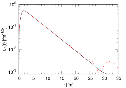
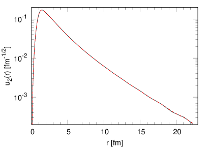
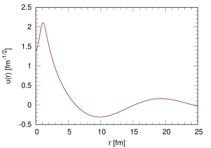
Figure 1: The deuteron $u_{0}(r)$ (left top panel) and $u_{2}(r)$ (right top panel) functions, and the $nn$ ${}^{1}S_{0}$ function (left bottom panel) at $E=5$ MeV are calculated with the variational (dashed red line) and the Numerov (black line) methods. The NVIa potential is used. In order to appreciate the differences between the two methods, the function $u_{0}(r)$ and $u_{2}(r)$ are shown in semilogarithmic scale.

III Results

We present in this section the results for the $\Gamma^{D}(^{1}S_{0})$ muon capture rate, obtained using the Norfolk potentials and consistent currents, as presented in Sec. II.2. In particular, we will use the four Norfolk potentials NVIa, NVIb, NVIIa, and NVIIb, obtained varying the short- and long-range cutoffs (models a or b), and the range of laboratory energies over which the fits have been carried out (models I or II). For each model, the weak vector current and the axial current and charge operators have been consistently constructed. In particular, we will indicate with the label LO those results obtained including only the LO contributions in the vector current and axial current and charge operators, with NLO those ones obtained including, in addition, the NLO contributions to the vector current and axial charge operators. In fact, we remind that there are no NLO contributions to the axial current. With the label N2LO we will indicate those results obtained including the N2LO terms of the vector and axial currents, but not the axial charge, since they vanish exactly. Finally, with N3LO we will indicate the results obtained when N3LO terms in the vector and axial currents are retained. To be noticed that this is the order at which new LECs appear. The contribution at N3LO for the axial charge are instead discarded for the reasons explained in Sec. II.2. Finally, we will use for the axial single-nucleon form factor the dependence given in Eq. (3) with $g_{A}=1.2723$ and $r_{A}^{2}=0.46$ fm². However, in order to establish the uncertainty arising from the rather poor knowledge of $r_{A}^{2}$ (see Ref. Hill et al. (2018) and the discussion in Sec. I and at the end of Sec. II.2), we will show also results obtained with $r_{A}^{2}=0.30,0.46,0.62$ fm², so that the 0.16 fm² uncertainty on $r_{A}^{2}$ Hill et al. (2018) will be taken into account.

Firstly, we begin by proving that the uncertainty arising from the numerical method adopted to study the deuteron and the $nn$ scattering states is well below the 1% level. In fact, in Table 2 we present the results obtained with the NVIa potential and currents with up to N3LO contributions, using either the variational or the Numerov method to solve the two-body problem (see Sec. II.3). The function $d\Gamma^{D}(^{1}S_{0})/dp$ (see Eq. (4)) calculated with the same potential and currents is shown in Fig. 2. As it can be seen by inspection of the figure and the table, the agreement between the results obtained within the two methods is essentially perfect, of the order of 0.01 s^-1 in $\Gamma^{D}(^{1}S_{0})$, well below any other source of error ($\simeq 0.005\%$). Therefore, from now on, we will present only results obtained using the variational method, which is in fact numerically less involved than the Numerov one.

$\chi$-order	Numerov	Variational
LO	245.43	245.42
NLO	247.59	247.58
N2LO	254.67	254.65
N3LO	255.31	255.30

Table 2: The total doublet capture rate in the ${}^{1}S_{0}$ $nn$ channel, $\Gamma^{D}(^{1}S_{0})$ in s^-1, calculated using either the Numerov or the variational methods to obtain the deuteron and the $nn$ scattering wave functions. Here we report the results up to the digit for which the two methods differ. The NVIa potential and consistent currents at the various chiral order are used, and the axial charge radius is taken to be $r_{A}^{2}=0.46$ fm².

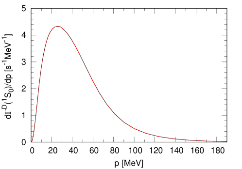
Figure 2: The differential doublet capture rate in the ${}^{1}S_{0}$ $nn$ channel, $d\Gamma^{D}(^{1}S_{0})/dp$ in s^-1MeV^-1, as function of the $nn$ relative momentum $p$ in MeV, calculated using either the Numerov (black solid line) or the variational (red dashed line) methods in order to obtain the deuteron and the $nn$ scattering wave functions. The curves are exactly on the top of each other. The NVIa potential and consistent currents at N3LO are used. The axial charge radius is taken to be $r_{A}^{2}=0.46$ fm².

We now present in Table 3 the results for $\Gamma^{D}(^{1}S_{0})$, obtained using all the four Norfolk potentials, NVIa, NVIb, NVIIa and NVIIb, and consistent currents, from LO, up to N3LO. The axial charge radius is fixed at $r_{A}^{2}=0.46$ fm². By inspection of the table, we can provide our best estimate for $\Gamma^{D}({{}^{1}S_{0}})$, which we calculate simply as the average between the four values at N3LO, $\Gamma^{D}(^{1}S_{0})=$ 255.8 s^-1. Furthermore, we would like to remark that the overall model-dependence is quite small, the largest difference being of the order of 1.1 s^-1 between the NVIa and NVIIb results, at N3LO. Going into more detail, (i) by comparing the NVIa (NVIIa) and NVIb (NVIIb) results, still at N3LO, we can get a grasp on the cutoff dependence, which turns out to be smaller than 1 s^-1 for both models I and II. (ii) By comparing the NVIa (NVIb) and NVIIa (NVIIb) results, also in this case at N3LO, we can conclude that the dependence on the $NN$ database used for the LECs fitting procedure in the potentials is essentially of the same order. To remain conservative, we have decided to define the theoretical uncertainty arising from model-dependence as the half range, i.e.

$$\Delta\Gamma^{D}(^{1}S_{0})[{\rm mod-dep}]\equiv\frac{|\Gamma^{D}(^{1}S_{0})_{\rm NVIIb}-\Gamma^{D}(^{1}S_{0})_{\rm NVIa}|}{2}\ .$$ (72)

From this we obtain $\Delta\Gamma^{D}(^{1}S_{0})[{\rm mod-dep}]=0.6$ s^-1.

Still by inspection of Table 3, we can conclude that the chiral order convergence seems to be quite well under control for all the potential models. In fact, in going from LO to NLO, $\Gamma^{D}(^{1}S_{0})$ has increased by 2.2 s^-1 for the a models, and 2.5 s^-1 and 2.4 s^-1 for the models NVIb and NVIIb, respectively. This small change is due to the fact that the only correction appearing at NLO comes from the vector current. Passing from NLO to N2LO the muon capture rate increases of 7.1 s^-1 for the interactions NVIa and NVIIa, and 11.5 s^-1 and 11.3 s^-1 for the models NVIb and NVIIb, respectively. This can be understood considering that the terms with the $\Delta$-isobar contributions appear at this order for the vector and axial current. The convergence at N3LO shows instead a more involved behaviour: for the models NVIa and NVIIa, $\Gamma^{D}(^{1}S_{0})$ increase of 0.6 s^-1 and 0.9 s^-1 respectively while for the models NVIb and NVIIb the muon capture rate decreases of 3.5 s^-1 and 3.9 s^-1, respectively. Even if the results are in reasonable agreement with the expected chiral convergence behaviour (in particular for the models a), the chiral convergence of the current shows a significant dependence on the regularization, that we tracked back to the axial current corrections and in particular to the different value of the constant $c_{D}$ (see Section II.2). We find still remarkable that the results at N3LO obtained with the various potentials, even if their chiral convergence pattern are quite different, turn out to be within 1.1 s^-1.

The theoretical uncertainty arising from the chiral order convergence of the nuclear weak transition operators can be studied using the prescription of Ref. Epelbaum et al. (2015). Here we report the formula for the error at N2LO only. At this order, for each energy, we define the error for the differential capture rate (to symplify the notation from now on we use $\Gamma^{D}(p)=d\Gamma^{D}({}^{1}S_{0})/dp$), as

$$\Delta\Gamma^{D}(p)\equiv\max\left\{Q^{3}|\Gamma^{D}_{\rm LO}(p)|,\,Q^{2}|\Gamma^{D}_{\rm NLO}(p)-\Gamma^{D}_{\rm LO}(p)|,\,Q|\Gamma^{D}_{\rm N2LO}(p)-\Gamma^{D}_{\rm NLO}(p)|\right\}\ ,$$ (73)

where we have assumed

$$Q=\frac{1}{\Lambda}\frac{p^{8}+m_{\pi}^{8}}{p^{7}+m_{\pi}^{7}}$$ (74)

as in Ref. Acharya and Bacca (2022) for the case of the $np\leftrightarrow d\gamma$ reaction. Here, $p$ is the relative momentum of the $nn$ system and we assume a value of $\Lambda\simeq 550$ MeV, which is of the order of the cutoff of the adopted interactions. Analogous formula have been used to study the other orders (see Ref. Epelbaum et al. (2015) for details).

In Fig. 3 we show the error on $d\Gamma^{D}(^{1}S_{0})/dp$ order by order in the expansion of the nuclear current up to N3LO for the NVIa interaction. From the figure it is evident the nice convergence of the chiral expansion.

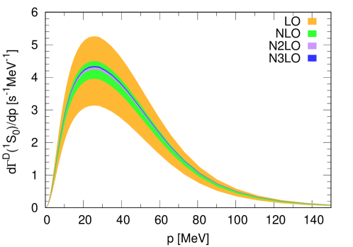
Figure 3: The differential doublet capture rate in the ${}^{1}S_{0}$ $nn$ channel, $d\Gamma^{D}(^{1}S_{0})/dp$ in s^-1MeV^-1, as function of the $nn$ relative momentum $p$ in MeV, calculated order by order with the relative errors computed following the prescription of Ref. Epelbaum et al. (2015). The axial charge radius is taken to be $r_{A}^{2}=0.46$ fm².

The total error arising from the chiral truncation of the currents on $\Gamma^{D}(^{1}S_{0})$ is then computed by integrating the error of the differential capture rate over $p$, namely

$$\Delta\Gamma^{D}({}^{1}S_{0})[\text{curr-conv}]=\int_{0}^{p_{max}}\Delta\Gamma^{D}(p)dp\,.$$ (75)

To be the most conservative possible we keep as error the largest obtained with the various interaction models. In the same spirit, we consider the error computed at N2LO, since the calculation at N3LO does not contain all the contributions of the axial charge (see discussion Section II.2). Therefore we obtain $\Delta\Gamma^{D}({}^{1}S_{0})[\text{curr-conv}]=4.4$ s^-1. In comparison the same calculation at N3LO would give as error $\Delta\Gamma^{D}({}^{1}S_{0})[\text{curr-conv}]|_{\rm N3LO}=1.4$ s^-1.

	Potentials
$\chi$-order	NVIa	NVIb	NVIIa	NVIIb
LO	245.4	245.1	245.7	246.6
NLO	247.6	247.6	247.9	249.0
N2LO	254.7	259.1	255.0	260.3
N3LO	255.3	255.6	255.9	256.4

Table 3: The total doublet capture rate in the ${}^{1}S_{0}$ $nn$ channel, $\Gamma^{D}(^{1}S_{0})$ in s^-1, calculated using the four Norfolk potentials NVIa, NVIb, NVIIa, and NVIIb, and consistent currents, at the various chiral orders. The axial charge radius is taken to be $r_{A}^{2}=0.46$ fm², and the variational method is applied in order to calculate the deuteron and the $nn$ scattering wave functions.

Finally, we present in Table 4 the results obtained with all the interactions and consistent currents up to N3LO for the three values of the axial charge radius, $r_{A}^{2}=0.30,0.46,0.62$ fm². This will allow us to understand the importance of this last source of theoretical uncertainty. The three values have been chosen to span the range of values proposed in Ref. Hill et al. (2018). Again, we define the theoretical uncertainty $\Delta\Gamma^{D}(^{1}S_{0})[r_{A}^{2}]$ arising from this last source as the half range of the results, i.e.

$$\Delta\Gamma^{D}(^{1}S_{0})[r_{A}^{2}]\equiv\max_{pot}\left\{\frac{|\Gamma^{D}(^{1}S_{0})_{r_{A}^{2}=0.30}-\Gamma^{D}(^{1}S_{0})_{r_{A}^{2}=0.62}|}{2}\right\}\ ,$$ (76)

where with $\max_{pot}$ we indicate that we take the maximum value among the different interactions considered. By inspection of the table, we can conclude that $\Delta\Gamma^{D}(^{1}S_{0})[r_{A}^{2}]=2.9$ s^-1, which is found to be essentially model-independent.

Pot.	$r_{A}^{2}=0.30$	$r_{A}^{2}=0.46$	$r_{A}^{2}=0.62$
NVIa	258.2	255.3	252.4
NVIb	258.5	255.6	252.8
NVIIa	258.7	255.9	253.0
NVIIb	259.3	256.4	253.6

Table 4: The total doublet capture rate in the ${}^{1}S_{0}$ $nn$ channel, $\Gamma^{D}(^{1}S_{0})$ in s^-1, is calculated using all the different interactions and consistent currents up to N3LO, and three different values of $r_{A}^{2}$, $r_{A}^{2}=0.30,0.46,0.62$ fm². The variational method is applied in order to calculate the deuteron and the $nn$ scattering wave functions.

In conclusion, our final result for $\Gamma^{D}(^{1}S_{0})$ is

$$\Gamma^{D}(^{1}S_{0})=255.8(0.6)(4.4)(2.9)\,\,{\rm s}^{-1}\ ,$$ (77)

where the three uncertainties arise from model-dependence, chiral convergence and the experimental error in the axial charge radius $r_{A}$. The overall systematic uncertainty becomes 5.0 s^-1, when the various contributions are summed. The uncertainty on $r_{A}^{2}$ is instead a statistical uncertainty and therefore must be treated separately. This result can be compared with those of Refs. Marcucci et al. (2012); Acharya et al. (2018). In Ref. Marcucci et al. (2012), we found a value of $253.5(1.2)$ s^-1, the error taking care of the cutoff dependence and the uncertainty in the $d_{R}$ LEC fitting procedure. When only the cutoff dependence is considered, it reduces to 0.2 s^-1, somewhat smaller than the present 0.6 s^-1. The central values that we have obtained and the one quoted in Ref. Marcucci et al. (2012), even if the chiral potentials are very different, are instead in reasonable agreement. In Ref. Acharya et al. (2018), it was found $\Gamma^{D}(^{1}S_{0})=252.8(4.6)(3.9)\;\rm{s}^{-1}$, where the first error is due to the truncation in the chiral expansion and the second to the uncertainty in the nucleon axial radius $r_{A}$. These two errors should be compared with our $5.0$ s^-1 and $2.9$ s^-1. The agreement for the first error is very nice, while the small difference in the second error is certainly due to the fact that in Ref. Acharya et al. (2018) a larger uncertainty for $r_{A}^{2}$ was used ($0.22$ fm² vs. the present $0.16$ fm²). Also in this case, the agreement between the central values is good, even if the potential models adopted are very different. This could suggest that the observable $\Gamma^{D}(^{1}S_{0})$ is not sensitive to the nuclear potential model, as long as this is able to properly reproduce the deuteron and the $nn$ scattering systems (as, in fact, any realistic modern potential usually does).

IV Conclusions and outlook

We have investigated, for the first time with local nuclear potential models derived in $\chi$EFT and consistent currents, the muon capture on deuteron, in the ${}^{1}S_{0}$ initial $nn$ scattering state. The use of this framework has allowed us to (i) provide a new estimate for the catpure rate $\Gamma^{D}(^{1}S_{0})$, which has turned out to be in agreement with the results already present in the literature and obtained still in $\chi$EFT, but with different (non-local) potential models Marcucci et al. (2012); Acharya et al. (2018); (ii) accompany this estimate with a determination of the theoretical uncertainty, which arises from model-dependence, chiral convergence, and the uncertainty in the single-nucleon axial charge radius $r_{A}$. We have also verified that the uncertainty arising from the numerical technique adopted to solve the two-body bound- and scattering-state problem is completely negligible. This is in contrast with the conclusions of Ref. Acharya et al. (2017), at least for the observable $\Gamma^{D}(^{1}S_{0})$.

Our final result is $\Gamma^{D}(^{1}S_{0})=255.8(0.6)(4.4)(2.9)$ s^-1, where the three errors come from the three sources of uncertainty just mentioned. In order to provide an indicative value for the overall uncertainty, we propose to sum the systematic uncertainties arising from source (i) and (ii), obtaining the value of 5.0 s^-1. Then, this error can be summed in quadrature with the one of source (iii), 2.9 s^-1. Therefore, we obtain $\Gamma^{D}(^{1}S_{0})=255.8(5.8)$ s^-1. We remark again that the value of 5.8 s^-1 for the overall uncertainty is only indicative, and the preferable procedure should be to treat the three errors, 0.6 s^-1, 4.4 s^-1, and 2.9 s^-1, separately.

Given the success of this calculation in determining $\Gamma^{D}(^{1}S_{0})$ and its uncertainty, with a procedure definitely less involved than the one of Ref. Acharya et al. (2018), which still leads to similar results, we plan to proceed applying this framework to the calculation of $\Gamma^{D}$, retaining all the $nn$ partial waves up to $J=2$ and $L=3$. These are known to provide contributions to $\Gamma^{D}$ up to 1 s^-1 Marcucci et al. (2011). In parallel, we plan to study the muon capture processes also on ³He and ⁶Li, on the footsteps of Ref. King et al. (2022a). Here the Norfolk potentials have been used in conjunction with the variational and Green’s function Monte Carlo techniques to solve for the $A=3,6$ bound states, and the final results have been found in some disagreement with the experimental data. It will be interesting to verify these outcomes, using the Hyperspherical Harmonics method to solve for the $A=3,6$ nuclei Marcucci et al. (2020); Gnech et al. (2020, 2021). Last but not least, we plan to apply this same framework to weak processes of interest for Solar standard models and Solar neutrino fluxes, i.e. the proton weak capture on proton (reaction 2), and on ³He (the so called $hep$ reaction). In this second case, it is remarkable that a consistent $\chi$EFT calculation is still missing (see Refs. Marcucci et al. (2001); Park et al. (2003); Adelberger et al. (2011)). For both reactions, we will be able to provide a value for the astrophysical $S$-factor at zero energy accompanied by an estimate of the theoretical uncertainty.

Conflict of Interest Statement

The authors declare that the research was conducted in the absence of any commercial or financial relationships that could be construed as a potential conflict of interest.

Author Contributions

LC and LEM have shared the idea, the formula derivation and the computer code implementation of the work presented here. LEM has also taken the main responsibility for the drafting of the manuscript. AG has contributed in reviewing the codes and running them in order to obtain the final results presented here, while MP and MV have given valuable suggestions during the setting up of the calculation. All the Authors have equally contributed in reviewing and correcting the draft of the manuscript.

Funding

The support by the U.S. Departmentof Energy, Office of Nuclear Science, under ContractsNo. DE-AC05-06OR23177 is acknowledged by AG, while the U.S. Department ofEnergy through the FRIB Theory Alliance Award No. DE-SC0013617 is acknowledged by MP.

References

- Measday (2001) Measday DF. The nuclear physics of muon capture. Phys. Rep. 354 (2001) 243.
- Wang et al. (1965) Wang IT, Anderson EW, Bleser EJ, Lederman LM, Meyer SL, Rosen JL, et al. Muon capture in (p d)+ molecules. Phys. Rev. 139 (1965) B1528.
- Bertin et al. (1973) Bertin A, Vitale A, Placci A, Zavattini E. Muon capture in gaseous deuterium. Phys. Rev. D 8 (1973) 3774.
- Bardin et al. (1986) Bardin G, Duclos J, Martino J, Bertin A, Capponi M, Piccinini M, et al. A measurement of the muon capture rate in liquid deuterium by the lifetime technique. Nucl. Phys. A 453 (1986) 591.
- Cargnelli M, et al. (1989) Cargnelli M, et al. Workshop on fundamental physics, Los Alamos, 1986, LA 10714C. Nuclear weak process and nuclear structure, Yamada Conference XXIII, edited by M. Morita, H. Ejiri, H. Ohtsubo, and T. Sato, World Scientific, Singapore (1989) 115.
- Kammel (2013) Kammel P. Precision muon capture at PSI. PoS CD12 (2013) 016.
- Marcucci (2012) Marcucci LE. Muon capture on deuteron and 3He: A personal review. Int. J. Mod. Phys. A 27 (2012) 1230006.
- Adam et al. (2012) Adam J Jr, Tater M, Truhlik E, Epelbaum E, Machleidt R, Ricci P. Calculation of Doublet Capture Rate for Muon Capture in Deuterium within Chiral Effective Field Theory. Phys. Lett. B 709 (2012) 93.
- Marcucci et al. (2011) Marcucci LE, Piarulli M, Viviani M, Girlanda L, Kievsky A, Rosati S, et al. Muon capture on deuteron and . Phys. Rev. C 83 (2011) 014002.
- Marcucci et al. (2012) Marcucci LE, Kievsky A, Rosati S, Schiavilla R, Viviani M. Chiral effective field theory predictions for muon capture on deuteron and 3He. Phys. Rev. Lett. 108 (2012) 052502. [Erratum: Phys. Rev. Lett. 121, (2018) 049901].
- Golak et al. (2014) Golak J, Skibiński R, Witała H, Topolnicki K, Elmeshneb AE, Kamada H, et al. Break-up channels in muon capture on 3He. Phys. Rev. C 90 (2014) 024001. [Addendum: Phys.Rev.C 90, 029904 (2014)].
- Acharya et al. (2018) Acharya B, Ekström A, Platter L. Effective-field-theory predictions of the muon-deuteron capture rate. Phys. Rev. C 98 (2018) 065506.
- Entem and Machleidt (2003) Entem DR, Machleidt R. Accurate charge dependent nucleon nucleon potential at fourth order of chiral perturbation theory. Phys. Rev. C 68 (2003) 041001.
- Machleidt and Entem (2011) Machleidt R, Entem DR. Chiral effective field theory and nuclear forces. Phys. Rept. 503 (2011) 1.
- Gazit et al. (2009) Gazit D, Quaglioni S, Navrátil P. Three-Nucleon Low-Energy Constants from the Consistency of Interactions and Currents in Chiral Effective Field Theory. Phys. Rev. Lett. 103 (2009) 102502. [Erratum: Phys. Rev. Lett. 122, (2019) 029901].
- Carlsson et al. (2016) Carlsson BD, Ekström A, Forssén C, Strömberg DF, Jansen GR, Lilja O, et al. Uncertainty analysis and order-by-order optimization of chiral nuclear interactions. Phys. Rev. X 6 (2016) 011019.
- Acharya et al. (2017) Acharya B, Ekström A, Odell D, Papenbrock T, Platter L. Corrections to nucleon capture cross sections computed in truncated Hilbert spaces. Phys. Rev. C 95 (2017) 031301.
- Piarulli and Tews (2020) Piarulli M, Tews I. Local nucleon-nucleon and three-nucleon interactions within chiral effective field theory. Front. Phys. 7 (2020) 245.
- Piarulli et al. (2016) Piarulli M, Girlanda L, Schiavilla R, Kievsky A, Lovato A, Marcucci LE, et al. Local chiral potentials with -intermediate states and the structure of light nuclei. Phys. Rev. C 94 (2016) 054007.
- Baroni et al. (2018) Baroni A, Schiavilla R, Marcucci LE, Girlanda L, Kievsky A, Lovato A, et al. Local chiral interactions, the tritium Gamow-Teller matrix element, and the three-nucleon contact term. Phys. Rev. C 98 (2018) 044003.
- Schiavilla et al. (2019) Schiavilla R, Baroni A, Pastore S, Piarulli M, Girlanda L, Kievsky A, et al. Local chiral interactions and magnetic structure of few-nucleon systems. Phys. Rev. C 99 (2019) 034005.
- Gnech and Schiavilla (2022) Gnech A, Schiavilla R. Magnetic structure of few-nucleon systems at high momentum transfers in a EFT approach (2022). arXiv:2207.05528.
- Piarulli et al. (2018) Piarulli M, et al. Light-nuclei spectra from chiral dynamics. Phys. Rev. Lett. 120 (2018) 052503. doi:10.1103/PhysRevLett.120.052503.
- Gandolfi et al. (2020) Gandolfi S, Lonardoni D, Lovato A, Piarulli M. Atomic nuclei from quantum Monte Carlo calculations with chiral EFT interactions. Front. in Phys. 8 (2020) 117.
- King et al. (2020a) King GB, Andreoli L, Pastore S, Piarulli M, Schiavilla R, Wiringa RB, et al. Chiral Effective Field Theory Calculations of Weak Transitions in Light Nuclei. Phys. Rev. C 102 (2020a) 025501.
- King et al. (2020b) King GB, Andreoli L, Pastore S, Piarulli M. Weak Transitions in Light Nuclei. Front. in Phys. 8 (2020b) 363.
- King et al. (2022a) King GB, Pastore S, Piarulli M, Schiavilla R. Partial muon capture rates in A=3 and A=6 nuclei with chiral effective field theory. Phys. Rev. C 105 (2022a) L042501.
- Cirigliano et al. (2019) Cirigliano V, Dekens W, De Vries J, Graesser ML, Mereghetti E, Pastore S, et al. Renormalized approach to neutrinoless double- decay. Phys. Rev. C 100 (2019) 055504.
- King et al. (2022b) King GB, Baroni A, Cirigliano V, Gandolfi S, Hayen L, Mereghetti E, et al. Ab initio calculation of the decay spectrum of 6He (2022b). ArXiv:2207.11179.
- Piarulli et al. (2020) Piarulli M, Bombaci I, Logoteta D, Lovato A, Wiringa RB. Benchmark calculations of pure neutron matter with realistic nucleon-nucleon interactions. Phys. Rev. C 101 (2020) 045801.
- Lovato et al. (2022) Lovato A, Bombaci I, Logoteta D, Piarulli M, Wiringa RB. Benchmark calculations of infinite neutron matter with realistic two- and three-nucleon potentials. Phys. Rev. C 105 (2022).
- Acharya et al. (2019) Acharya B, Platter L, Rupak G. Universal behavior of -wave proton-proton fusion near threshold. Phys. Rev. C 100 (2019) 021001.
- Marcucci et al. (2013) Marcucci LE, Schiavilla R, Viviani M. Proton-Proton Weak Capture in Chiral Effective Field Theory. Phys. Rev. Lett. 110 (2013) 192503. [Erratum: Phys. Rev. Lett. 123, (2019) 019901].
- Hill et al. (2018) Hill RJ, Kammel P, Marciano WJ, Sirlin A. Nucleon axial radius and muonic hydrogen—a new analysis and review. Rep. Prog. Phys. 81 (2018) 096301.
- Walecka (1995) Walecka J. Theorethical Nuclear and Subnuclear Physics (London: Imperial College Press) (1995).
- Navarro Pérez et al. (2013) Navarro Pérez R, Amaro JE, Ruiz Arriola E. Coarse-grained potential analysis of neutron-proton and proton-proton scattering below the pion production threshold. Phys. Rev. C 88 (2013) 064002. [Erratum: Phys. Rev. C 91, (2015) 029901].
- Navarro Pérez et al. (2014a) Navarro Pérez R, E AJ, Ruiz Arriola E. Coarse grained potential with chiral two-pion exchange. Phys. Rev. C 89 (2014a) 024004.
- Navarro Pérez et al. (2014b) Navarro Pérez R, E AJ, Ruiz Arriola E. Statistical error analysis for phenomenological nucleon-nucleon potentials. Phys. Rev. C 89 (2014b) 064006.
- Krebs et al. (2007) Krebs H, Epelbaum E, Meissner U. Nuclear forces with excitations up to next-to-next-to-leading order, part I: Peripheral nucleon-nucleon waves. Eur. Phys. J. A 32 (2007) 127.
- Baroni et al. (2016) Baroni A, Girlanda L, Pastore S, Schiavilla R, Viviani M. Nuclear axial currents in chiral effective field theory. Phys. Rev. C 93 (2016) 015501.
- Meyer et al. (2016) Meyer AS, Betancourt M, Gran R, Hill RJ. Deuterium target data for precision neutrino-nucleus cross sections. Phys. Rev. D 93 (2016) 113015.
- Abramowitz and Stegun (1964) Abramowitz M, Stegun IA. Handbook of mathematical functions with formulas, graphs, and mathematical tables, vol. 55 (US Government printing office) (1964).
- Kohn (1948) Kohn W. Variational methods in nuclear collision problems. Phys. Rev. 74 (1948) 1763.
- Johnson (1978) Johnson BR. The renormalized Numerov method applied to calculating bound states of the coupled-channel Schroedinger equation. J. Chem. Phys. 69 (1978) 4678.
- Epelbaum et al. (2015) Epelbaum E, Krebs H, UG M. Improved chiral nucleon-nucleon potential up to next-to-next-to-next-to-leading order. Eur. Phys. J. A 51 (2015) 53.
- Acharya and Bacca (2022) Acharya B, Bacca S. Gaussian process error modeling for chiral effective-field-theory calculations of at low energies. Phys. Lett. B 827 (2022) 137011.
- Marcucci et al. (2020) Marcucci LE, Dohet-Eraly J, Girlanda L, Gnech A, Kievsky A, Viviani M. The Hyperspherical Harmonics method: a tool for testing and improving nuclear interaction models. Front. in Phys. 8 (2020) 69.
- Gnech et al. (2020) Gnech A, Viviani M, Marcucci LE. Calculation of the 6Li ground state within the hyperspherical harmonic basis. Phys. Rev. C 102 (2020) 014001.
- Gnech et al. (2021) Gnech A, Marcucci LE, Schiavilla R, Viviani M. Comparative study of 6He -decay based on different similarity-renormalization-group evolved chiral interactions. Phys. Rev. C 104 (2021) 035501.
- Marcucci et al. (2001) Marcucci LE, Schiavilla R, Viviani M, Kievsky A, Rosati S, Beacom JF. Weak proton capture on 3He. Phys. Rev. C 63 (2001) 015801.
- Park et al. (2003) Park TS, Marcucci LE, Schiavilla R, Viviani M, Kievsky A, Rosati S, et al. Parameter free effective field theory calculation for the solar proton fusion and hep processes. Phys. Rev. C 67 (2003) 055206.
- Adelberger et al. (2011) Adelberger EG, et al. Solar fusion cross sections II: the pp chain and CNO cycles. Rev. Mod. Phys. 83 (2011) 195.