Mean-square convergence and stability of the backward Euler method for stochastic differential delay equations with highly nonlinear growing coefficients

Abstract

Over the last few decades, the numerical methods for stochastic differential delay equations (SDDEs) have been investigated and developed by many scholars. Nevertheless, there is still little work to be completed. By virtue of the novel technique, this paper focuses on the mean-square convergence and stability of the backward Euler method (BEM) for SDDEs whose drift and diffusion coefficients can both grow polynomially. The upper mean-square error bounds of BEM are obtained. Then the convergence rate, which is one-half, is revealed without using the moment boundedness of numerical solutions. Furthermore, under fairly general conditions, the novel technique is applied to prove that the BEM can inherit the exponential mean-square stability with a simple proof. At last, two numerical experiments are implemented to illustrate the reliability of the theories.

Keywords: The backward Euler method; Stochastic differential delay equations; Mean-square convergence; Mean-square stability

1 Introduction

Stochastic differential equations (SDEs) have been investigated by many scholars due to their extensive applications in many fields, including control problems, finance, biology, population model, communication, etc [1, 20, 28]. However, it is difficult to obtain the exact solutions to SDEs. So using numerical algorithms to aquire approximations is a meaningful way to analyze the properties of solutions. It is well known that Euler-Maruyama (EM) method is one of the most popular numerical algorithms for SDEs [20, 28]. Unfortunately, the divergence of EM scheme for SDEs with super-linear coefficients was proved in [18]. Whereafter, different kinds of modified EM methods have been established to approximate nonlinear SDEs, such as truncated EM method[24, 29], tamed EM method[19, 38], stopped EM method[26], multilevel EM method[3], projected EM method[5] and others. Furthermore, the implicit methods have also been studied and developed on account of their better convergence rates in the last decades [2, 4, 20, 40, 44].

The scholars use stochastic differential delay equations(SDDEs) to describe a class of more applicative systems which not only depend on the present state but also depend on the past state[6, 28]. Like SDEs, the numerical methods of SDDEs have also been widely discussed. The modified EM methods for SDDEs were analyzed in[11, 9, 13, 22, 39], while the implicit EM methods were investigated in [12, 25, 41, 43, 50]. It is worth noting that the diffusion coefficients of the equations in [12, 25, 41, 43, 50] can not grow super-linearly, which has a adverse effect on the development of the implicit methods. In order to eliminate this adverse effect, the papers [52, 49, 53] and [46, 48] focused on studying the backward Euler method (BEM) and split-step method for SDDEs respectively, whose drift and diffusion coefficients can grow super-linearly. However, the convergence rate was not shown in [52]; there is no constant in the diffusion coefficient in [49, 53], which is a strong constraint. Therefore, by exploiting the novel technique, the first goal of our paper is to investigate the strong convergence rate of the BEM for SDDEs with highly nonlinear drift and diffusion coefficients under the weaker conditions.

As is known to all, in addition to the convergence, the long-time stability of the numerical solution is also worth studying. The stabilities of implicit EM methods for SDEs were given in [14, 16, 30, 32]. In the rest of this paragraph, we only discuss the stability of the implicit scheme for SDDEs. When the diffusion coefficients satisfy $|g(x(t),x(t-\tau))|^{2}\leq c_{1}|x(t)|^{2}+c_{2}|x(t-\tau)|^{2}$ (where $c_{1},c_{2}$ are positive constants and $x(t-\tau)$ is the delay term), the stabilities of the BEM solutions to SDDEs were studied in [10, 17, 23, 33, 34, 37, 42, 45, 47, 54]. The theories in [49, 52, 53] can not cover the equations with diffusion coefficient $g(x(t),x(t-\tau))=x(t-\tau)$. Similarly, to a degree, Assumption 2.2 in [8] is also a bit strong. Moreover, the stabilities of split-step methods were analyzed in [7, 51, 35, 50, 43]. Especially, it should be noted that the constraint of coefficients was relaxed in [55], but the locally Lipschitz conditions of coefficients were used in the proof process. Hence, the second goal of our paper is to prove that the numerical solutions to BEM for SDDEs are exponentially mean-square stable without using the locally Lipschitz conditions. That is, by making use of the novel technique, the mean-square stability of the numerical solutions can be obtained easily under the weaker conditions .

Let’s summarize the main contributions of our paper. Under the fairly general conditions, by borrowing the techniques from[2, 27, 44], we investigate the strong convergence rate and exponential mean-square stability of the BEM for SDDEs whose drift and diffusion coefficients can grow super-linearly.

To use the novel technique, we introduce the crucial equality

$$2\langle x-y,x\rangle=|x|^{2}-|y|^{2}+|x-y|^{2},~{}~{}~{}~{}~{}~{}~{}\forall x,y\in\mathbb{R}^{d},$$ (1.1)

which will play an important role in our paper. Moreover, the discussions of the comparison between explicit and implicit numerical schemes can be found in [15, 21, 27, 44] and references therein.

This paper is organized as follows. In Section 2, we introduce some necessary notations and prove that the global error in mean-square sence is controlled by the local error. Section 3 gives the convergence rate of BEM without using the moment boundedness of numerical solutions. In Section 4, under a stronger condition, the convergence rate is given by a much simpler proof. In Section 5, we present the exponential mean-square stability of BEM. In Section 6, two numerical examples are considered to illustrate the reliability of the theories.

2 Error bounds for BEM

Let $|\cdot|$ and$<\cdot,\cdot>$ denote the Euclidean norm and the inner product of vectors in $\mathbb{R}^{d}$. We use $\mathbb{N}$ to denote the set of all positive integers. If $A\in\mathbb{R}^{d\times m}$ is a matrix, its trace norm is denoted by$\|A\|=\sqrt{trace(A^{T}A)}$, where $A^{T}$ is the transpose of matrix A, $d,m\in\mathbb{N}$. Let $\big{(}\Omega,\mathcal{F},\{\mathcal{F}_{t}\}_{t\in[0,T]},\mathbb{P}\big{)}$ stand for a complete probability space with a filtration $\{\mathcal{F}_{t}\}_{t\in[0,T]}$ satisfying the usual conditions (i.e., it is increasing and right continuous while $\mathcal{F}_{0}$ contains all $\mathbb{P}$-null sets). Let $\mathbb{E}$ be the probability expectation with respect to $\mathbb{P}$. Let $\mathcal{L}^{r}=\mathcal{L}^{r}(\Omega,\mathbb{R}^{d})$ be the family of $\mathbb{R}^{d}$-valued random variables $\xi$ satisfying $\mathbb{E}|\xi|^{r}<\infty$, $r\in\mathbb{N}$. Let $\mathcal{C}([-\tau,0];\mathbb{R}^{d})$ stand for the family of all continuous functions from $[-\tau,0]$ to $\mathbb{R}^{d}$ with the norm $|\varphi|_{\infty}=\sup_{-\tau\leq\theta\leq 0}|\varphi(\theta)|$. And denote by C a generic positive constant which is independent of time stepsize.

Now we consider the nonlinear SDDE of the form

$$dx(t)=\alpha\left(x(t),x(t-\tau)\right)dt+\beta\left(x(t),x(t-\tau)\right)dW(t),$$ (2.1)

on $t\geq 0$ with the initial data

$$x_{0}=\varphi=\{\varphi(\theta):-\tau\leq\theta\leq 0\}\in\mathcal{C}([-\tau,0];\mathbb{R}^{d}),$$ (2.2)

where $\alpha:\mathbb{R}^{d}\times\mathbb{R}^{d}\rightarrow\mathbb{R}^{d}$ and $\beta:\mathbb{R}^{d}\times\mathbb{R}^{d}\rightarrow\mathbb{R}^{d\times m}$. Moreover, $W(t)$ is an m-dimensional Brownian motion.

Now we construct the BEM for SDDEs. Suppose that there exist two positive integers $N,M$ such that $\Delta=\frac{T}{N}=\frac{\tau}{M}$, where $\Delta$ is the step size. Define

$$\left\{\begin{array}[]{l}Z_{n}=\varphi(n\Delta),~{}~{}~{}~{}~{}~{}~{}~{}~{}~{}~{}n=-M,-M+1,...,0,\\ Z_{n}=Z_{n-1}+\alpha(Z_{n},Z_{n-M})\Delta+\beta(Z_{n-1},Z_{n-1-M})\Delta W_{n-1},~{}~{}n=1,2,...,N,\end{array}\right.$$ (2.5)

where $\Delta W_{n-1}:=W(t_{n})-W(t_{n-1})$.

Before analyzing the errors between exact solutions and numerical solutions, some necessary assumptions should be imposed.

Assumption 2.1.

There exist constants $K>0$ and $q>2$ such that

$$\begin{split}&\langle x-\bar{x},\alpha(x,y)-\alpha(\bar{x},\bar{y})\rangle+\frac{(q-1)}{2}\|\beta(x,y)-\beta(\bar{x},\bar{y})\|^{2}\\ \leq&K(|x-\bar{x}|^{2}+|y-\bar{y}|^{2}),\end{split}$$

for any $x,y,\bar{x},\bar{y}\in\mathbb{R}^{d}$.

By Assumption 2.1, we can get that

$$\langle x-\bar{x},\alpha(x,y)-\alpha(\bar{x},y)\rangle\leq K|x-\bar{x}|^{2},$$ (2.6)

for any $x,y,\bar{x}\in\mathbb{R}^{d}$. When $K\Delta<1$, (2.5) has a unique solution due to the fixed point theorem. Then the BEM is well defined [32].

Assumption 2.2.

Suppose that the SDDE (2.1) admits a unique $\{\mathcal{F}_{t}\}_{t\in[0,T]}$-adapted solution with continuous sample paths, and $\sup_{s\in[0,T]}\mathbb{E}|x(s)|^{2}<\infty$, $\sup_{s\in[0,T]}\mathbb{E}|\alpha(x(s),x(s-\tau))|^{2}<\infty$ hold. Furthermore, assume that the BEM admits a unique $\{\mathcal{F}_{t_{n}}\}_{n\in\{1,2,\cdots,N\}}$-adapted solution$\{Z_{n}\}_{n=0}^{N}$ as well.

Lemma 2.3.

Let Assumption 2.2 hold. For ${n\in\{1,2,...,N\}}$, $N\in\mathbb{N}$, we have

$$\begin{split}&\big{|}[x(t_{n})-Z_{n}]-\Delta[\alpha(x(t_{n}),x(t_{n-M}))-\alpha(Z_{n},Z_{n-M})]\big{|}^{2}\\ =&\big{|}[x(t_{n-1})-Z_{n-1}]-\Delta[\alpha(x(t_{n-1}),x(t_{n-1-M}))-\alpha(Z_{n-1},Z_{n-1-M})]\big{|}^{2}\\ &-\Delta^{2}\big{|}\alpha(x(t_{n-1}),x(t_{n-1-M}))-\alpha(Z_{n-1},Z_{n-1-M})\big{|}^{2}\\ &+\big{|}[\beta(x(t_{n-1}),x(t_{n-1-M}))-\beta(Z_{n-1},Z_{n-1-M})]\Delta W_{n-1}\big{|}^{2}+|\mathcal{R}_{n}|^{2}\\ &+2\Delta\langle x(t_{n-1})-Z_{n-1},\alpha(x(t_{n-1}),x(t_{n-1-M}))-\alpha(Z_{n-1},Z_{n-1-M})\rangle\\ &+2\langle[x(t_{n-1})-Z_{n-1}]-\Delta[\alpha(x(t_{n-1}),x(t_{n-1-M}))-\alpha(Z_{n-1},Z_{n-1-M})],\\ &~{}~{}~{}~{}~{}~{}[\beta(x(t_{n-1}),x(t_{n-1-M}))-\beta(Z_{n-1},Z_{n-1-M})]\Delta W_{n-1}\rangle\\ &+2\langle[x(t_{n-1})-Z_{n-1}]-\Delta[\alpha(x(t_{n-1}),x(t_{n-1-M}))-\alpha(Z_{n-1},Z_{n-1-M})],\mathcal{R}_{n}\rangle\\ &+2\Delta\langle\alpha(x(t_{n-1}),x(t_{n-1-M}))-\alpha(Z_{n-1},Z_{n-1-M}),\\ &~{}~{}~{}~{}~{}~{}~{}~{}[\beta(x(t_{n-1}),x(t_{n-1-M}))-\beta(Z_{n-1},Z_{n-1-M})]\Delta W_{n-1}\rangle\\ &+2\Delta\langle\alpha(x(t_{n-1}),x(t_{n-1-M}))-\alpha(Z_{n-1},Z_{n-1-M}),\mathcal{R}_{n}\rangle\\ &+2\langle[\beta(x(t_{n-1}),x(t_{n-1-M}))-\beta(Z_{n-1},Z_{n-1-M})]\Delta W_{n-1},\mathcal{R}_{n}\rangle,\end{split}$$ (2.7)

where

$$\begin{split}\mathcal{R}_{n}=&\int_{t_{n-1}}^{t_{n}}[\alpha(x(s),x(s-\tau))-\alpha(x(t_{n})-x(t_{n-M}))]ds\\ &+\int_{t_{n-1}}^{t_{n}}[\beta(x(s),x(s-\tau))-\beta(x(t_{n-1})-x(t_{n-1-M}))]dW(s).\end{split}$$ (2.8)

Proof.

From the definitions of (2.1) and (2.5), one can see that

$$\begin{split}&[x(t_{n})-Z_{n}]-\Delta[\alpha(x(t_{n}),x(t_{n-M}))-\alpha(Z_{n},Z_{n-M})]\\ =&[x(t_{n-1})-Z_{n-1}]-\Delta[\alpha(x(t_{n-1}),x(t_{n-1-M}))-\alpha(Z_{n-1},Z_{n-1-M})]\\ &+\Delta[\alpha(x(t_{n-1}),x(t_{n-1-M}))-\alpha(Z_{n-1},Z_{n-1-M})]\\ &+[\beta(x(t_{n-1}),x(t_{n-1-M}))-\beta(Z_{n-1},Z_{n-1-M})]\Delta W_{n-1}\\ &+\mathcal{R}_{n},\end{split}$$

where $\mathcal{R}_{n}$ is defined by (2.8). Then we have

$$\begin{split}&\big{|}[x(t_{n})-Z_{n}]-\Delta[\alpha(x(t_{n}),x(t_{n-M}))-\alpha(Z_{n},Z_{n-M})]\big{|}^{2}\\ =&\big{|}[x(t_{n-1})-Z_{n-1}]-\Delta[\alpha(x(t_{n-1}),x(t_{n-1-M}))-\alpha(Z_{n-1},Z_{n-1-M})]\big{|}^{2}\\ &+\Delta^{2}\big{|}\alpha(x(t_{n-1}),x(t_{n-1-M}))-\alpha(Z_{n-1},Z_{n-1-M})\big{|}^{2}\\ &+\big{|}[\beta(x(t_{n-1}),x(t_{n-1-M}))-\beta(Z_{n-1},Z_{n-1-M})]\Delta W_{n-1}\big{|}^{2}+|\mathcal{R}_{n}|^{2}\\ &+2\Delta\langle x(t_{n-1})-Z_{n-1},\alpha(x(t_{n-1}),x(t_{n-1-M}))-\alpha(Z_{n-1},Z_{n-1-M})\rangle\\ &-2\Delta^{2}\big{|}\alpha(x(t_{n-1}),x(t_{n-1-M}))-\alpha(Z_{n-1},Z_{n-1-M})\big{|}^{2}\\ &+2\langle[x(t_{n-1})-Z_{n-1}]-\Delta[\alpha(x(t_{n-1}),x(t_{n-1-M}))-\alpha(Z_{n-1},Z_{n-1-M})],\\ &~{}~{}~{}~{}~{}~{}[\beta(x(t_{n-1}),x(t_{n-1-M}))-\beta(Z_{n-1},Z_{n-1-M})]\Delta W_{n-1}\rangle\\ &+2\langle[x(t_{n-1})-Z_{n-1}]-\Delta[\alpha(x(t_{n-1}),x(t_{n-1-M}))-\alpha(Z_{n-1},Z_{n-1-M})],\mathcal{R}_{n}\rangle\\ &+2\Delta\langle\alpha(x(t_{n-1}),x(t_{n-1-M}))-\alpha(Z_{n-1},Z_{n-1-M}),\\ &~{}~{}~{}~{}~{}~{}~{}~{}~{}[\beta(x(t_{n-1}),x(t_{n-1-M}))-\beta(Z_{n-1},Z_{n-1-M})]\Delta W_{n-1}\rangle\\ &+2\Delta\langle\alpha(x(t_{n-1}),x(t_{n-1-M}))-\alpha(Z_{n-1},Z_{n-1-M}),\mathcal{R}_{n}\rangle\\ &+2\langle[\beta(x(t_{n-1}),x(t_{n-1-M}))-\beta(Z_{n-1},Z_{n-1-M})]\Delta W_{n-1},\mathcal{R}_{n}\rangle.\end{split}$$

Rearranging the above equation gives the result. ∎

Lemma 2.4.

Let Assumptions 2.1,2.2 hold and $0<2K\Delta<1$. Then for all $n\in\{1,2,...,N\}$, $N\in\mathbb{N}$, we derive that

$$\mathbb{E}\big{|}\mathcal{R}_{n}\big{|}^{2}<\infty,~{}~{}~{}~{}~{}~{}~{}~{}\mathbb{E}\big{|}x(t_{n})-Z_{n}\big{|}^{2}<\infty,$$

$$\mathbb{E}\big{|}[x(t_{n})-Z_{n}]-\Delta[\alpha(x(t_{n}),x(t_{n-M}))-\alpha(Z_{n},Z_{n-M})]\big{|}^{2}<\infty,$$

$$\mathbb{E}\big{|}\alpha(x(t_{n}),x(t_{n-M}))-\alpha(Z_{n},Z_{n-M})\big{|}^{2}<\infty,$$

$$\mathbb{E}\|\beta(x(t_{n}),x(t_{n-M}))-\beta(Z_{n},Z_{n-M})]\Delta W_{n-1}\|^{2}<\infty.$$

Proof.

For all $n\in\{1,2,...,N\}$, $N\in\mathbb{N}$ , we prove $\mathbb{E}|\mathcal{R}_{n}|^{2}<\infty$ firstly. We have already known that $\sup_{s\in[0,T]}\mathbb{E}|x(s)|^{2}<\infty$ and $\sup_{s\in[0,T]}\mathbb{E}|\alpha(x(s),x(s-\tau))|^{2}<\infty$. By Assumption 2.1, for $s\in[t_{n-1},t_{n}]$ we can get

$$\begin{split}&\mathbb{E}\big{\|}\beta(x(s),x(s-\tau))-\beta(x(t_{n-1})-x(t_{n-1-M}))\big{\|}^{2}\\ \leq&\frac{2K}{(q-1)}\mathbb{E}\big{|}x(s)-x(t_{n-1})\big{|}^{2}+\frac{2K}{(q-1)}\mathbb{E}\big{|}x(s-\tau)-x(t_{n-1-M})\big{|}^{2}\\ &-\frac{2}{(q-1)}\mathbb{E}\big{\langle}x(s)-x(t_{n-1}),\alpha(x(s),x(s-\tau))-\alpha(x(t_{n-1}),x(t_{n-1-M}))\big{\rangle}\\ \leq&\frac{2K+1}{(q-1)}\mathbb{E}\big{|}x(s)-x(t_{n-1})\big{|}^{2}+\frac{2K}{(q-1)}\mathbb{E}\big{|}x(s-\tau)-x(t_{n-1-M})\big{|}^{2}\\ &+\frac{1}{(q-1)}\mathbb{E}\big{|}\alpha(x(s),x(s-\tau))-\alpha(x(t_{n-1}),x(t_{n-1-M}))\big{|}^{2}<\infty.\end{split}$$

Relying on the obtained information above, for ${n\in\{1,2,...,N\}}$, $N\in\mathbb{N}$, $\mathbb{E}|\mathcal{R}_{n}|^{2}<\infty$ can be proved due to the Itô isometry. Taking expectations on both sides of (2.7), it is easy to get

$$\begin{split}&\mathbb{E}\big{|}[x(t_{n})-Z_{n}]-\Delta[\alpha(x(t_{n}),x(t_{n-M}))-\alpha(Z_{n},Z_{n-M})]\big{|}^{2}\\ \leq&2\mathbb{E}\big{|}[x(t_{n-1})-Z_{n-1}]-\Delta[\alpha(x(t_{n-1}),x(t_{n-1-M}))-\alpha(Z_{n-1},Z_{n-1-M})]\big{|}^{2}\\ &+2\mathbb{E}\big{\|}[\beta(x(t_{n-1}),x(t_{n-1-M}))-\beta(Z_{n-1},Z_{n-1-M})]\Delta W_{n-1}\big{\|}^{2}+4\mathbb{E}|\mathcal{R}_{n}|^{2}\\ &+2\Delta\mathbb{E}\big{\langle}x(t_{n-1})-Z_{n-1},\alpha(x(t_{n-1}),x(t_{n-1-M}))-\alpha(Z_{n-1},Z_{n-1-M})\big{\rangle}\\ &+2\mathbb{E}\big{\langle}[x(t_{n-1})-Z_{n-1}]-\Delta[\alpha(x(t_{n-1}),x(t_{n-1-M}))-\alpha(Z_{n-1},Z_{n-1-M})],\\ &~{}~{}~{}~{}~{}~{}~{}~{}~{}~{}[\beta(x(t_{n-1}),x(t_{n-1-M}))-\beta(Z_{n-1},Z_{n-1-M})]\Delta W_{n-1}\big{\rangle}\\ &+2\Delta\mathbb{E}\big{\langle}\alpha(x(t_{n-1}),x(t_{n-1-M}))-\alpha(Z_{n-1},Z_{n-1-M}),\\ &~{}~{}~{}~{}~{}~{}~{}~{}~{}~{}~{}[\beta(x(t_{n-1}),x(t_{n-1-M}))-\beta(Z_{n-1},Z_{n-1-M})]\Delta W_{n-1}\big{\rangle}.\\ \end{split}$$ (2.9)

Next, we use the inductive reasoning to prove
$\mathbb{E}\big{|}[x(t_{n})-Z_{n}]-\Delta[\alpha(x(t_{n}),x(t_{n-M}))-\alpha(Z_{n},Z_{n-M})]\big{|}^{2}<\infty$. One can observe that

$$\begin{split}&[x(0)-Z_{0}]-\Delta[\alpha(x(0),x(-\tau))-\alpha(Z_{0},Z_{-M})]\\ =&[\alpha(x(0),x(-\tau))-\alpha(Z_{0},Z_{-M})]\\ =&\alpha(x(0),x(-\tau))-\alpha(Z_{0},Z_{-M})\\ =&[\beta(x(0),x(-\tau))-\beta(Z_{0},Z_{-M})]\Delta W_{0}\\ =&0.\end{split}$$

According to (2.9), we konw that $\mathbb{E}\big{|}[x(t_{1})-Z_{1}]-\Delta[\alpha(x(t_{1}),x(t_{1-M}))-\alpha(Z_{1},Z_{1-M})]\big{|}^{2}\leq 4\mathbb{E}|\mathcal{R}_{1}|^{2}<\infty$. Now we suppose that
$\mathbb{E}\big{|}[x(t_{n-1})-Z_{n-1}]-\Delta[\alpha(x(t_{n-1}),x(t_{n-1-M}))-\alpha(Z_{n-1},Z_{n-1-M})]\big{|}^{2}<\infty$, then we get from Assumption 2.1 that

$$\begin{split}&\mathbb{E}\big{|}[x(t_{n-1})-Z_{n-1}]-\Delta[\alpha(x(t_{n-1}),x(t_{n-1-M}))-\alpha(Z_{n-1},Z_{n-1-M})]\big{|}^{2}\\ =&\mathbb{E}\big{|}x(t_{n-1})-Z_{n-1}\big{|}^{2}\\ &-2\Delta\mathbb{E}\big{\langle}x(t_{n-1})-Z_{n-1},\alpha(x(t_{n-1}),x(t_{n-1-M}))-\alpha(Z_{n-1},Z_{n-1-M})\big{\rangle}\\ &+\Delta^{2}\mathbb{E}\big{|}\alpha(x(t_{n-1}),x(t_{n-1-M}))-\alpha(Z_{n-1},Z_{n-1-M})\big{|}^{2}\\ \geq&\mathbb{E}\big{|}x(t_{n-1})-Z_{n-1}\big{|}^{2}\\ &-2K\Delta\mathbb{E}\big{|}x(t_{n-1})-Z_{n-1}\big{|}^{2}-2K\Delta\mathbb{E}\big{|}x(t_{n-1-M})-Z_{n-1-M}\big{|}^{2}\\ &+\Delta^{2}\mathbb{E}\big{|}\alpha(x(t_{n-1}),x(t_{n-1-M}))-\alpha(Z_{n-1},Z_{n-1-M})\big{|}^{2}.\end{split}$$

Thus,

$$\begin{split}&\mathbb{E}\big{|}[x(t_{n-1})-Z_{n-1}]-\Delta[\alpha(x(t_{n-1}),x(t_{n-1-M}))-\alpha(Z_{n-1},Z_{n-1-M})]\big{|}^{2}\\ &+2K\Delta\mathbb{E}\big{|}x(t_{n-1-M})-Z_{n-1-M}\big{|}^{2}\\ \geq&(1-2K\Delta)\mathbb{E}\big{|}x(t_{n-1})-Z_{n-1}\big{|}^{2}\\ &+\Delta^{2}\mathbb{E}\big{|}\alpha(x(t_{n-1}),x(t_{n-1-M}))-\alpha(Z_{n-1},Z_{n-1-M})\big{|}^{2}.\end{split}$$

Based on the assumptions above, we have

$$\begin{split}\infty>&(1-2K\Delta)\mathbb{E}\big{|}x(t_{n-1})-Z_{n-1}\big{|}^{2}\\ &+\Delta^{2}\mathbb{E}\big{|}\alpha(x(t_{n-1}),x(t_{n-1-M}))-\alpha(Z_{n-1},Z_{n-1-M})\big{|}^{2}.\end{split}$$

Therefore, for $0\leq 2K\varDelta<1$, one can derive that

$$\begin{split}&\mathbb{E}\big{|}x(t_{n-1})-Z_{n-1}\big{|}^{2}<\infty,\\ &\mathbb{E}\big{|}\alpha(x(t_{n-1}),x(t_{n-1-M}))-\alpha(Z_{n-1},Z_{n-1-M})\big{|}^{2}<\infty,\end{split}$$

and

$$\begin{split}&\mathbb{E}\big{\|}\beta(x(t_{n-1}),x(t_{n-1-M}))-\beta(Z_{n-1},Z_{n-1-M})\big{\|}^{2}\\ \leq&\frac{2K+1}{(q-1)}\mathbb{E}\big{|}x(t_{n-1})-Z_{n-1}\big{|}^{2}+\frac{2K}{(q-1)}\mathbb{E}\big{|}x(t_{n-1-M})-Z_{n-1-M}\big{|}^{2}\\ &+\frac{1}{(q-1)}\mathbb{E}\big{|}\alpha(x(t_{n-1}),x(t_{n-1-M}))-\alpha(Z_{n-1},Z_{n-1-M})\big{|}^{2}<\infty.\end{split}$$

Moreover, using the properties of Brownian motion and Itô’s isometry gives that

$$\begin{split}&\mathbb{E}\big{|}[\beta(x(t_{n-1}),x(t_{n-1-M}))-\beta(Z_{n-1},Z_{n-1-M})]\Delta W_{n-1}\big{|}^{2}\\ =&\Delta\mathbb{E}\big{\|}\beta(x(t_{n-1}),x(t_{n-1-M}))-\beta(Z_{n-1},Z_{n-1-M})\big{\|}^{2},\\ &\mathbb{E}\big{\langle}[x(t_{n-1})-Z_{n-1}]-\Delta[\alpha(x(t_{n-1}),x(t_{n-1-M}))-\alpha(Z_{n-1},Z_{n-1-M})],\\ &~{}~{}~{}~{}[\beta(x(t_{n-1}),x(t_{n-1-M}))-\beta(Z_{n-1},Z_{n-1-M})]\Delta W_{n-1}\big{\rangle}=0,\\ &\mathbb{E}\big{\langle}\alpha(x(t_{n-1}),x(t_{n-1-M}))-\alpha(Z_{n-1},Z_{n-1-M}),\\ &~{}~{}~{}~{}[\beta(x(t_{n-1}),x(t_{n-1-M}))-\beta(Z_{n-1},Z_{n-1-M})]\Delta W_{n-1}\big{\rangle}=0.\end{split}$$

Using Assumption 2.1, we get from (2.9) that

$$\begin{split}&\mathbb{E}\big{|}[x(t_{n})-Z_{n}]-\Delta[\alpha(x(t_{n}),x(t_{n-M}))-\alpha(Z_{n},Z_{n-M})]\big{|}^{2}]\\ \leq&2\mathbb{E}\big{|}[x(t_{n-1})-Z_{n-1}]-\Delta[\alpha(x(t_{n-1}),x(t_{n-1-M}))-\alpha(Z_{n-1},Z_{n-1-M})]\big{|}^{2}\\ &+2\Delta\mathbb{E}\big{\|}\beta(x(t_{n-1}),x(t_{n-1-M}))-\beta(Z_{n-1},Z_{n-1-M})\big{\|}^{2}+4\mathbb{E}|\mathcal{R}_{n}|^{2}\\ &+2\Delta\mathbb{E}\big{\langle}x(t_{n-1})-Z_{n-1},\alpha(x(t_{n-1}),x(t_{n-1-M}))-\alpha(Z_{n-1},Z_{n-1-M})\big{\rangle}\\ \leq&2\mathbb{E}\big{|}[x(t_{n-1})-Z_{n-1}]-\Delta[\alpha(x(t_{n-1}),x(t_{n-1-M}))-\alpha(Z_{n-1},Z_{n-1-M})]\big{|}^{2}\\ &+2\Delta\mathbb{E}\big{\|}\beta(x(t_{n-1}),x(t_{n-1-M}))-\beta(Z_{n-1},Z_{n-1-M})\big{\|}^{2}+4\mathbb{E}|\mathcal{R}_{n}|^{2}\\ &+2K\Delta\mathbb{E}\big{|}x(t_{n-1})-Z_{n-1}\big{|}^{2}+2K\Delta\mathbb{E}\big{|}x(t_{n-1-M})-Z_{n-1-M}\big{|}^{2}<\infty.\end{split}$$

By the induction reasoning, we know that $\mathbb{E}\big{|}[x(t_{n})-Z_{n}]-\Delta[\alpha(x(t_{n}),x(t_{n-M}))-\alpha(Z_{n},Z_{n-M})]\big{|}^{2}<\infty$. Then for for all $n\in\{1,2,...,N\}$ , $N\in\mathbb{N}$, the following results can be acquired

$$\mathbb{E}\big{|}x(t_{n})-Z_{n}\big{|}^{2}<\infty,$$

$$\mathbb{E}\big{|}\alpha(x(t_{n}),x(t_{n-M}))-\alpha(Z_{n},Z_{n-M})\big{|}^{2}<\infty,$$

$$\mathbb{E}\big{\|}\beta(x(t_{n}),x(t_{n-M}))-\beta(Z_{n},Z_{n-M})\big{\|}^{2}<\infty.$$

∎

With these two lemmas, we are going to prove the following theorem.

Theorem 2.5.

Let Assumptions 2.1, 2.2 hold and $0<2K\Delta<1$. Then for all $n\in\{1,2,...,N\}$, $N\in\mathbb{N}$, there is a constant $C$ independent of n , such that

$$\mathbb{E}|x(t_{n})-Z_{n}|^{2}\leq C\left(\sum_{i=1}^{n}\mathbb{E}|\mathcal{R}_{i}|^{2}+\Delta^{-1}\sum_{i=1}^{n}\mathbb{E}\big{[}|\mathbb{E}(\mathcal{R}_{i}\mid\mathcal{F}_{t_{i-1}})|^{2}\big{]}\right),$$

where $\mathcal{R}_{i}$ is defined by (2.8).

Proof.

By Lemma 2.3 and the Hölder inequality, we derive that

$$\begin{split}&\mathbb{E}\big{|}[x(t_{n})-Z_{n}]-\Delta[\alpha(x(t_{n}),x(t_{n-M}))-\alpha(Z_{n},Z_{n-M})]\big{|}^{2}\\ \leq&\mathbb{E}\big{|}[x(t_{n-1})-Z_{n-1}]-\Delta[\alpha(x(t_{n-1}),x(t_{n-1-M}))-\alpha(Z_{n-1},Z_{n-1-M})]\big{|}^{2}\\ &+\Delta\mathbb{E}\big{\|}\beta(x(t_{n-1}),x(t_{n-1-M}))-\beta(Z_{n-1},Z_{n-1-M})\big{\|}^{2}+\mathbb{E}|\mathcal{R}_{n}|^{2}\\ &+2\Delta\mathbb{E}\big{\langle}x(t_{n-1})-Z_{n-1},\alpha(x(t_{n-1}),x(t_{n-1-M}))-\alpha(Z_{n-1},Z_{n-1-M})\big{\rangle}\\ &+2\mathbb{E}\big{\langle}[x(t_{n-1})-Z_{n-1}]-\Delta[\alpha(x(t_{n-1}),x(t_{n-1-M}))-\alpha(Z_{n-1},Z_{n-1-M})],\mathcal{R}_{n}\big{\rangle}\\ &+2\Delta\mathbb{E}\big{\langle}\alpha(x(t_{n-1}),x(t_{n-1-M}))-\alpha(Z_{n-1},Z_{n-1-M}),\mathcal{R}_{n}\big{\rangle}\\ &+(q-2)\mathbb{E}\big{\|}[\beta(x(t_{n-1}),x(t_{n-1-M}))-\beta(Z_{n-1},Z_{n-1-M})]\Delta W_{n-1}\big{\|}^{2}\\ &+\frac{1}{q-2}\mathbb{E}|\mathcal{R}_{n}|^{2}\\ =&\mathbb{E}\big{|}[x(t_{n-1})-Z_{n-1}]-[\alpha(x(t_{n-1}),x(t_{n-1-M}))-\alpha(Z_{n-1},Z_{n-1-M})]\big{|}^{2}\\ &+2\Delta\mathbb{E}\big{\langle}x(t_{n-1})-Z_{n-1},\alpha(x(t_{n-1}),x(t_{n-1-M}))-\alpha(Z_{n-1},Z_{n-1-M})\big{\rangle}\\ &+(q-1)\Delta\mathbb{E}\big{|}\beta(x(t_{n-1}),x(t_{n-1-M}))-\beta(Z_{n-1},Z_{n-1-M})\big{|}^{2}+\frac{q-1}{q-2}\mathbb{E}|\mathcal{R}_{n}|^{2}\\ &+2\mathbb{E}\big{\langle}x(t_{n-1})-Z_{n-1},\mathcal{R}_{n}\big{\rangle}.\\ \end{split}$$

Using Assumption 2.1 and the properties of conditional expectation leads to

$$\begin{split}\mathbb{E}&\big{|}[x(t_{n})-Z_{n}]-\Delta[\alpha(x(t_{n}),x(t_{n-M}))-\alpha(Z_{n},Z_{n-M})]\big{|}^{2}\\ \leq&\mathbb{E}\big{|}[x(t_{n-1})-Z_{n-1}]-\Delta[\alpha(x(t_{n-1}),x(t_{n-1-M}))-\alpha(Z_{n-1},Z_{n-1-M})]\big{|}^{2}\\ &+2K\Delta\mathbb{E}\big{|}x(t_{n-1})-Z_{n-1}\big{|}^{2}+2K\Delta\mathbb{E}\big{|}x(t_{n-1-M})-Z_{n-1-M}\big{|}^{2}\\ &+\Delta\mathbb{E}\big{|}x(t_{n-1})-Z_{n-1}\big{|}^{2}+\frac{1}{\Delta}\mathbb{E}\big{[}|\mathbb{E}(\mathcal{R}_{i}\mid\mathcal{F}_{t_{i-1}})|^{2}\big{]}+\frac{q-1}{q-2}\mathbb{E}|\mathcal{R}_{n}|^{2}.\end{split}$$

By iterating and $\mathbb{E}\big{|}[x(t_{0})-Z_{0}]-\Delta[\alpha(x(t_{0}),x(-\tau))-\alpha(Z_{0},Z_{-M})]\big{|}=0$, we have

$$\begin{split}&\mathbb{E}\big{|}[x(t_{n})-Z_{n}]-\Delta[\alpha(x(t_{n}),x(t_{n-M}))-\alpha(Z_{n},Z_{n-M})]\big{|}^{2}\\ \leq&\mathbb{E}\big{|}[x(t_{0})-Z_{0}]-\Delta[\alpha(x(t_{0}),x(-\tau))-\alpha(Z_{0},Z_{-M})]\big{|}^{2}\\ &+(2K+1)\Delta\sum_{i=0}^{n-1}\mathbb{E}\big{|}x(t_{i})-Z_{i}\big{|}^{2}+2K\Delta\sum_{i=0}^{n-1}\mathbb{E}\big{|}x(t_{i-M})-Z_{i-M}\big{|}^{2}\\ &+\frac{1}{\Delta}\sum_{i=1}^{n}\mathbb{E}\big{[}|\mathbb{E}(\mathcal{R}_{i}\mid\mathcal{F}_{t_{i-1}})|^{2}\big{]}+\frac{q-1}{q-2}\sum_{i=1}^{n}\mathbb{E}|\mathcal{R}_{i}|^{2}\\ \leq&(2K+1)\Delta\sum_{i=0}^{n-1}\mathbb{E}\big{|}x(t_{i})-Z_{i}\big{|}^{2}+2K\Delta\sum_{i=-M}^{n-1-M}\mathbb{E}\big{|}x(t_{i})-Z_{i}\big{|}^{2}\\ &+\frac{1}{\Delta}\sum_{i=1}^{n}\mathbb{E}\big{[}|\mathbb{E}(\mathcal{R}_{i}\mid\mathcal{F}_{t_{i-1}})|^{2}\big{]}+\frac{q-1}{q-2}\sum_{i=1}^{n}\mathbb{E}|\mathcal{R}_{i}|^{2},\\ \end{split}$$

where we used the fact that $\sum_{i=0}^{n-1}\mathbb{E}\big{|}x(t_{i-M})-Z_{i-M}\big{|}^{2}=\sum_{i=-M}^{n-1-M}\mathbb{E}\big{|}x(t_{i})-Z_{i}\big{|}^{2}.$ Using the Assumption 2.1 leads to

$$\begin{split}&\mathbb{E}\big{|}[x(t_{n})-Z_{n}]-\Delta[\alpha(x(t_{n}),x(t_{n-M}))-\alpha(Z_{n},Z_{n-M})]\big{|}^{2}\\ =&\mathbb{E}\big{|}x(t_{n})-Z_{n}\big{|}^{2}-2\Delta\mathbb{E}\big{\langle}x(t_{n})-Z_{n},\alpha(x(t_{n}),x(t_{n-M}))-\alpha(Z_{n},Z_{n-M})\big{\rangle}\\ &+\Delta^{2}\mathbb{E}\big{|}\alpha(x(t_{n}),x(t_{n-M}))-\alpha(Z_{n},Z_{n-M})\big{|}^{2}\\ \geq&(1-2K\Delta)\mathbb{E}\big{|}x(t_{n})-Z_{n}\big{|}^{2}-2K\Delta\mathbb{E}\big{|}x(t_{n-M})-Z_{n-M}\big{|}^{2}.\end{split}$$

Combining these inequalities yields that

$$\begin{split}&(1-2K\Delta)\mathbb{E}\big{|}x(t_{n})-Z_{n}\big{|}^{2}\\ \leq&(2K+1)\Delta\sum_{i=0}^{n-1}\mathbb{E}\big{|}x(t_{i})-Z_{i}\big{|}^{2}+2K\Delta\sum_{i=-M}^{-1}\mathbb{E}\big{|}x(t_{i})-Z_{i}\big{|}^{2}\\ &+2K\Delta\sum_{i=0}^{n-1-M}\mathbb{E}\big{|}x(t_{i})-Z_{i}\big{|}^{2}+2K\Delta\mathbb{E}\big{|}x(t_{n-M})-Z_{n-M}\big{|}^{2}\\ &+\frac{1}{\Delta}\sum_{i=1}^{n}\mathbb{E}\big{[}|\mathbb{E}(\mathcal{R}_{i}\mid\mathcal{F}_{t_{i-1}})|^{2}\big{]}+\frac{q-1}{q-2}\sum_{i=1}^{n}\mathbb{E}|\mathcal{R}_{i}|^{2}\\ \leq&(2K+1)\Delta\sum_{i=0}^{n-1}\mathbb{E}\big{|}x(t_{i})-Z_{i}\big{|}^{2}+2K\Delta\sum_{i=0}^{n-M}\mathbb{E}\big{|}x(t_{i})-Z_{i}\big{|}^{2}\\ &+\frac{1}{\Delta}\sum_{i=1}^{n}\mathbb{E}\big{[}|\mathbb{E}(\mathcal{R}_{i}\mid\mathcal{F}_{t_{i-1}})|^{2}\big{]}+\frac{q-1}{q-2}\sum_{i=1}^{n}\mathbb{E}|\mathcal{R}_{i}|^{2}\\ \leq&(4K+1)\Delta\sum_{i=0}^{n-1}\mathbb{E}\big{|}x(t_{i})-Z_{i}\big{|}^{2}+\frac{1}{\Delta}\sum_{i=1}^{n}\mathbb{E}\big{[}|\mathbb{E}(\mathcal{R}_{i}\mid\mathcal{F}_{t_{i-1}})|^{2}\big{]}+\frac{q-1}{q-2}\sum_{i=1}^{n}\mathbb{E}|\mathcal{R}_{i}|^{2}.\\ \end{split}$$

By the Gronwall inequality, we get the desired result.

∎

3 Strong convergence rate

The strong convergence rate of BEM for SDDE with super-linear coefficients is dicussed in this section. In order to analyze the convergence rate, we need to make additional assumptions.

Assumption 3.1.

Let Assumption 2.1 hold, and there are several constants $\rho\in[1,\infty)$, $\bar{p}\in[4\rho-2,\infty)$, $K_{1}\in(0,\infty)$ such that

$$\big{|}\alpha(x,y)-\alpha(\bar{x},\bar{y})\big{|}\leq K_{1}\big{(}1+|x|^{\rho-1}+|y|^{\rho-1}+|\bar{x}|^{\rho-1}+|\bar{y}|^{\rho-1}\big{)}\big{(}|x-\bar{x}|+|y-\bar{y}|\big{)}$$

$$\big{\langle}x,\alpha(x,y)\big{\rangle}+\frac{(\bar{p}-1)}{2}\big{\|}\beta(x,y)\big{\|}^{2}\leq K_{1}\big{(}1+|x|^{2}+|y|^{2}\big{)},$$

for any $x,y,\bar{x},\bar{y}\in\mathbb{R}^{d}$.

By Young’s inequality, Assumption 3.1 leads to

$$\begin{split}&\|\beta(x,y)-\beta(\bar{x},\bar{y})\|^{2}\leq C(1+|x|^{\rho-1}+|y|^{\rho-1}+|\bar{x}|^{\rho-1}+|\bar{y}|^{\rho-1})(|x-\bar{x}|^{2}+|y-\bar{y}|^{2}),\end{split}$$ (3.1)

$$|(\alpha(x,y)|\leq C\left(1+|x|^{\rho}+|y|^{\rho}\right),$$

and

$$\|(\beta(x,y)\|^{2}\leq C\left(1+|x|^{\rho+1}+|y|^{\rho+1}\right),$$ (3.2)

for any $x,y,\bar{x},\bar{y}\in\mathbb{R}^{d}$.

It is worth noting that Assumption 3.1 suffices to imply Assumption 2.2, which means that SDDE (2.1) admits a unique solution satisfying $\sup_{s\in[0,T]}\mathbb{E}|x(s)|^{2}<\infty$, $\sup_{s\in[0,T]}\mathbb{E}\big{|}\alpha(x(s),x(s-\tau))\big{|}^{2}<\infty$. Moreover, under Assumption 3.1, for any $p\in[2,\bar{p}]$, the exact solution of SDDE (2.1) with the initial data (2.2) satisfies

$$\sup_{t\in[0,T]}\mathbb{E}|x(t)|^{p}<\infty.$$

Assumption 3.2.

There exists a constant $K_{2}>0$ such that the initial value $\varphi$ satisfies

$$|\varphi({\theta_{2}})-\varphi({\theta_{1}})|\leq K_{2}|{\theta_{2}}-{\theta_{1}}|^{\frac{1}{2}},~{}~{}~{}~{}~{}~{}~{}-\tau\leq{\theta_{1}}<{\theta_{2}}\leq 0.$$

Lemma 3.3.

Let Assumption 3.1 hold. For any $0\leq t_{1}<t_{2}\leq T$ , we can derive that

$$\left(\mathbb{E}\left|x(t_{2})-x(t_{1})\right|^{\gamma}\right)^{\frac{1}{\gamma}}\leq C(t_{2}-t_{1})^{\frac{1}{2}},~{}~{}~{}~{}~{}\forall\gamma\in[2,\bar{p}/\rho].$$

Proof.

Using an elementary inequality $|a+b|^{\gamma}\leq 2^{\gamma-1}(|a|^{\gamma}+|b|^{\gamma})$ for any $a,b\in\mathbb{R}^{d}$, it is easy to get that

$$\begin{split}&\mathbb{E}\left|x(t_{2})-x(t_{1})\right|^{\gamma}\\ \leq&2^{\gamma-1}\mathbb{E}\left|\int_{t_{1}}^{t_{2}}\alpha\left(x(s),x(s-\tau)\right)ds\right|^{\gamma}+2^{\gamma-1}\mathbb{E}\left|\int_{t_{1}}^{t_{2}}\beta\left(x(s),x(s-\tau)\right)dW(s)\right|^{\gamma}.\end{split}$$

Then by Assumption 3.1, Hölder’s inequality and Theorem 1.7.1 in [28], one can derive that

$$\begin{split}&\mathbb{E}\left|x(t_{2})-x(t_{1})\right|^{\gamma}\\ \leq&[2(t_{2}-t_{1})]^{\gamma-1}\mathbb{E}\int_{t_{1}}^{t_{2}}|\alpha\left(x(s),x(s-\tau)\right)|^{\gamma}ds\\ &+\frac{1}{2}[2\gamma(\gamma-1)]^{\frac{\gamma}{2}}(t_{2}-t_{1})^{\frac{\gamma-2}{2}}\mathbb{E}\int_{t_{1}}^{t_{2}}|\beta\left(x(s),x(s-\tau)\right)|^{\gamma}ds\\ \leq&C(t_{2}-t_{1})^{\gamma-1}\int_{t_{1}}^{t_{2}}\mathbb{E}\left(1+|x(s)|^{\gamma\rho}+|x(s-\tau)|^{\gamma\rho}\right)ds\\ &+C(t_{2}-t_{1})^{\frac{\gamma-2}{2}}\int_{t_{1}}^{t_{2}}\mathbb{E}\left(1+|x(s)|^{\frac{\gamma(\rho+1)}{2}}+|x(s-\tau)|^{\frac{\gamma(\rho+1)}{2}}\right)ds\\ \leq&C(t_{2}-t_{1})^{\frac{\gamma}{2}}.\end{split}$$

∎

Theorem 3.4.

Let Assumption 3.1 hold and $\Delta\in(0,\frac{1}{2K})$. Then for the exact solution x(t) to SDDE(2.1) and the numerical solution $Z_{n}$ to BEM(2.5), there is a constant $C$ independent of n, $\Delta$ such that

$$\sup_{0\leq n\leq N}\mathbb{E}|x(t_{n})-Z_{n}|^{2}\leq C\Delta.$$

Proof.

According to Theorem 2.5, to obtain the convergence rate, what we need to do is estimating two terms $\mathbb{E}[|\mathbb{E}(\mathcal{R}_{i}\mid\mathcal{F}_{t_{i-1}})|^{2}]$ and $\mathbb{E}|\mathcal{R}_{i}|^{2}$, $i\in\{1,2,...,N\}$. By (2.8), we have

$$\begin{split}\mathbb{E}|\mathcal{R}_{i}|^{2}&=\mathbb{E}\Big{|}\int_{t_{i-1}}^{t_{i}}[\alpha(x(s),x(s-\tau))-\alpha(x(t_{i})-x(t_{i-M}))]ds\\ &+\int_{t_{i-1}}^{t_{i}}[\beta(x(s),x(s-\tau))-\beta(x(t_{i-1})-x(t_{i-1-M}))]dW(s)\Big{|}^{2}\\ \leq&2\mathbb{E}\Big{|}\int_{t_{i-1}}^{t_{i}}[\alpha(x(s),x(s-\tau))-\alpha(x(t_{i})-x(t_{i-M}))]ds\Big{|}^{2}\\ &+2\mathbb{E}\Big{|}\int_{t_{i-1}}^{t_{i}}[\beta(x(s),x(s-\tau))-\beta(x(t_{i-1})-x(t_{i-1-M}))]dW(s)\Big{|}^{2}.\\ \end{split}$$

Now we estimate the first term on the right side of the inequality. By the Hölder inequality and Assumptions 3.1, 3.2, we can get

$$\begin{split}&\mathbb{E}\left|\int_{t_{i-1}}^{t_{i}}[\alpha(x(s),x(s-\tau))-\alpha(x(t_{i})-x(t_{i-M}))]ds\right|^{2}\\ \leq&C\Delta\mathbb{E}\int_{t_{i-1}}^{t_{i}}\left|\alpha(x(s),x(s-\tau))-\alpha(x(t_{i})-x(t_{i-M}))\right|^{2}ds\\ \leq&C\Delta\int_{t_{i-1}}^{t_{i}}\mathbb{E}\Big{[}(1+|x(s)|^{2\rho-2}+|x(s-\tau)|^{2\rho-2}+|x(t_{i})|^{2\rho-2}+|x(t_{i-M})|^{2\rho-2})\\ &~{}~{}~{}~{}~{}~{}~{}~{}~{}~{}~{}~{}~{}~{}\cdot(|x(s)-x(t_{i})|^{2}+|x(s-\tau)-x(t_{i-M})|^{2})\Big{]}ds\\ \leq&C\Delta\int_{t_{i-1}}^{t_{i}}\big{(}1+\mathbb{E}|x(s)|^{\frac{\bar{p}(2\rho-2)}{\bar{p}-2\rho}}+\mathbb{E}|x(s-\tau)|^{\frac{\bar{p}(2\rho-2)}{\bar{p}-2\rho}}\\ &~{}~{}~{}~{}~{}~{}~{}~{}~{}~{}~{}~{}~{}~{}~{}+\mathbb{E}|x(t_{i})|^{\frac{\bar{p}(2\rho-2)}{\bar{p}-2\rho}}+\mathbb{E}|x(t_{i-M})|^{\frac{\bar{p}(2\rho-2)}{\bar{p}-2\rho}}\big{)}^{\frac{\bar{p}-2\rho}{\bar{p}}}\\ &~{}~{}~{}~{}~{}~{}~{}~{}~{}~{}~{}~{}~{}\cdot\Big{[}\left(\mathbb{E}|x(s)-x(t_{i})|^{\frac{\bar{p}}{\rho}}\right)^{\frac{2\rho}{\bar{p}}}+\big{(}\mathbb{E}|x(s-\tau)-x(t_{i-M})|^{\frac{\bar{p}}{\rho}}\big{)}^{\frac{2\rho}{\bar{p}}}\Big{]}ds\\ \leq&C\Delta^{3}.\end{split}$$

Employing the Itô isometry gives that

$$\begin{split}&\mathbb{E}\left|\int_{t_{i-1}}^{t_{i}}[\beta(x(s),x(s-\tau))-\beta(x(t_{i-1})-x(t_{i-1-M}))]dW(s)\right|^{2}\\ =&\mathbb{E}\int_{t_{i-1}}^{t_{i}}\big{\|}\beta(x(s),x(s-\tau))-\beta(x(t_{i-1})-x(t_{i-1-M}))\big{\|}^{2}ds\\ \leq&C\int_{t_{i-1}}^{t_{i}}\mathbb{E}\Big{[}(1+|x(s)|^{\rho-1}+|x(s-\tau)|^{\rho-1}+|x(t_{i})|^{\rho-1}+|x(t_{i-M})|^{\rho-1})\\ &~{}~{}~{}~{}~{}~{}~{}~{}~{}~{}~{}~{}~{}\cdot(|x(s)-x(t_{i})|^{2}+|x(s-\tau)-x(t_{i-M})|^{2})\Big{]}ds\\ \leq&C\Delta^{2}.\end{split}$$

Thus, by Theorem 2.5, we draw a conclusion that

$$\mathbb{E}|\mathcal{R}_{i}|^{2}\leq K_{1}\Delta^{2}.$$ (3.3)

Moreover,

$$\begin{split}&\mathbb{E}\big{[}|\mathbb{E}(\mathcal{R}_{i}\mid\mathcal{F}_{t_{i-1}})|^{2}\big{]}\\ &=\mathbb{E}\Big{[}\big{|}\mathbb{E}\big{(}\int_{t_{i-1}}^{t_{i}}[\alpha(x(s),x(s-\tau))-\alpha(x(t_{i})-x(t_{i-M}))]ds\mid\mathcal{F}_{t_{i-1}}\big{)}\big{|}^{2}\Big{]}\\ &\leq\mathbb{E}\big{|}\int_{t_{i-1}}^{t_{i}}[\alpha(x(s),x(s-\tau))-\alpha(x(t_{i})-x(t_{i-M}))]ds\big{|}^{2}\\ &\leq C\Delta^{3},\end{split}$$ (3.4)

where we used the fact that

$$\mathbb{E}\left(\int_{t_{i-1}}^{t_{i}}[\beta(x(s),x(s-\tau))-\beta(x(t_{i-1})-x(t_{i-1-M}))]dW(s)\mid\mathcal{F}_{t_{i-1}}\right)=0.$$

Combining (3.3) and (3.4) gives the result. ∎

4 Convergence rate under the stronger condition

This section shows the convergence rate of BEM (2.5) for SDDE (2.1) under stronger condition by using a simpler proof process.

Assumption 4.1.

There exist constants $K_{3},K_{4}>0$ such that

$$\begin{split}&\langle x-\bar{x},\alpha(x,y)-\alpha(\bar{x},\bar{y})\rangle+\|\beta(x,y)-\beta(\bar{x},\bar{y})\|^{2}\\ \leq&-K_{3}|x-\bar{x}|^{2}+K_{4}|y-\bar{y}|^{2},\end{split}$$

for any $x,y,\bar{x},\bar{y}\in\mathbb{R}^{d}$.

Under Assumptions 3.1 and 4.1, (3.1) and (3.2) can be obtained similarly.

Theorem 4.2.

Let Assumptions 3.1, 4.1 hold and $\Delta\in(0,\frac{1}{K})$.Then for the exact solution x(t) to SDDE (2.1) and the numerical solution $Z_{n}$ to BEM (2.5), there is a constant $C$ independent of n, $\Delta$ satisfying

$$\sup_{0\leq n\leq N}\mathbb{E}|x(t_{n})-Z_{n}|^{2}\leq C\Delta.$$

Proof.

According to the definitions of (2.1) and (2.5), we have

$$\begin{split}&x(t_{n})-Z_{n}\\ =&[x(t_{n-1})-Z_{n-1}]+\Delta[\alpha(x(t_{n}),x(t_{n-M}))-\alpha(Z_{n},Z_{n-M})]\\ &+[\beta(x(t_{n-1}),x(t_{n-1-M}))-\beta(Z_{n-1},Z_{n-1-M})]\Delta W_{n-1}\\ &+\mathcal{R}_{n},\end{split}$$

where $\mathcal{R}_{n}$ is defined by (2.8). Then

$$\begin{split}&2\mathbb{E}\big{\langle}[x(t_{n})-Z_{n}]-[x(t_{n-1})-Z_{n-1}],x(t_{n})-Z_{n}\big{\rangle}\\ =&2\Delta\mathbb{E}\big{\langle}\alpha(x(t_{n}),x(t_{n-M}))-\alpha(Z_{n},Z_{n-M}),x(t_{n})-Z_{n}\big{\rangle}\\ &+2\mathbb{E}\big{\langle}[\beta(x(t_{n-1}),x(t_{n-1-M}))-\beta(Z_{n-1},Z_{n-1-M})]\Delta W_{n-1},x(t_{n})-Z_{n}\big{\rangle}\\ &+2\mathbb{E}\big{\langle}\mathcal{R}_{n},x(t_{n})-Z_{n}\big{\rangle}\\ =&2\Delta\mathbb{E}\big{\langle}\alpha(x(t_{n}),x(t_{n-M}))-\alpha(Z_{n},Z_{n-M}),x(t_{n})-Z_{n}\big{\rangle}\\ &+2\mathbb{E}\big{\langle}[\beta(x(t_{n-1}),x(t_{n-1-M}))-\beta(Z_{n-1},Z_{n-1-M})]\Delta W_{n-1},\\ &~{}~{}~{}~{}~{}[x(t_{n})-Z_{n}]-[x(t_{n-1})-Z_{n-1}]\big{\rangle}\\ &+2\mathbb{E}\big{\langle}\mathbb{E}\left(\mathcal{R}_{n}\mid\mathcal{F}_{t_{i-1}}\right),x(t_{n-1})-Z_{n-1}\big{\rangle}\\ &+2\mathbb{E}\big{\langle}\mathcal{R}_{n},[x(t_{n})-Z_{n}]-[x(t_{n-1})-Z_{n-1}]\big{\rangle}.\end{split}$$

By Young’s inequality and Assumption 4.1, there exists a positive constant $\varepsilon_{*}$ such that

$$\begin{split}&\mathbb{E}\big{|}x(t_{n})-Z_{n}\big{|}^{2}-\mathbb{E}\big{|}x(t_{n-1})-Z_{n-1}\big{|}^{2}+\mathbb{E}\big{|}[x(t_{n})-Z_{n}]-[x(t_{n-1})-Z_{n-1}]\big{|}^{2}\\ \leq&-2K_{3}\Delta\mathbb{E}\big{|}x(t_{n})-Z_{n}\big{|}^{2}+2K_{4}\Delta\mathbb{E}\big{|}x(t_{n-M})-Z_{n-M}\big{|}^{2}\\ &-2\Delta\mathbb{E}\big{\|}\beta(x(t_{n}),x(t_{n-M}))-\beta(Z_{n},Z_{n-M})\big{\|}^{2}\\ &+2\Delta\mathbb{E}\big{\|}\beta(x(t_{n-1}),x(t_{n-1-M}))-\beta(Z_{n-1},Z_{n-1-M})\big{\|}^{2}\\ &+2\mathbb{E}|\mathcal{R}_{n}|^{2}+\mathbb{E}\big{|}[x(t_{n})-Z_{n}]-[x(t_{n-1})-Z_{n-1}]\big{|}^{2}\\ &+\frac{1}{\varepsilon_{*}^{2}}\mathbb{E}\big{[}|\mathbb{E}(\mathcal{R}_{i}\mid\mathcal{F}_{t_{i-1}})|^{2}\big{]}+\varepsilon_{*}^{2}\mathbb{E}\big{|}x(t_{n-1})-Z_{n-1}\big{|}^{2},\end{split}$$

where we used the equliaty (1.1). Then the inequality can be rearranged as

$$\begin{split}&\big{(}1+2K_{3}\Delta\big{)}\mathbb{E}\big{|}x(t_{n})-Z_{n}\big{|}^{2}+2\Delta\mathbb{E}\big{\|}\beta(x(t_{n}),x(t_{n-M}))-\beta(Z_{n},Z_{n-M})\big{\|}^{2}\\ \leq&\big{(}1+\varepsilon_{*}^{2}\big{)}\mathbb{E}\big{|}x(t_{n-1})-Z_{n-1}\big{|}^{2}\\ &+2\Delta\mathbb{E}\big{\|}\beta(x(t_{n-1}),x(t_{n-1-M}))-\beta(Z_{n-1},Z_{n-1-M})\big{\|}^{2}\\ &+2K_{4}\Delta\mathbb{E}\big{|}x(t_{n-M})-Z_{n-M}\big{|}^{2}+2\mathbb{E}|\mathcal{R}_{n}|^{2}+\frac{1}{\varepsilon_{*}^{2}}\mathbb{E}\big{[}|\mathbb{E}(\mathcal{R}_{i}\mid\mathcal{F}_{t_{i-1}})|^{2}\big{]}.\end{split}$$ (4.1)

By choosing $\varepsilon_{*}=\sqrt{2K_{3}\Delta}$ and denoting ${G_{n}}=\big{(}1+2K_{3}\Delta\big{)}\mathbb{E}\big{|}x(t_{n})-Z_{n}\big{|}^{2}+2\Delta\mathbb{E}\big{\|}\beta(x(t_{n}),x(t_{n-M}))-\beta(Z_{n},Z_{n-M})\big{\|}^{2}$, we get that

$${G_{n}}-{G_{n-1}}\leq 2K_{4}\Delta\mathbb{E}\big{|}x(t_{n-M})-Z_{n-M}\big{|}^{2}+2\mathbb{E}|\mathcal{R}_{n}|^{2}+\frac{1}{2K_{3}\Delta}\mathbb{E}\big{[}|\mathbb{E}(\mathcal{R}_{i}\mid\mathcal{F}_{t_{i-1}})|^{2}\big{]}.$$

It is easy to see that

$$\begin{split}{G_{n}}\leq&2K_{4}\Delta\sum_{i=1}^{n}\mathbb{E}\big{|}x(t_{i-M})-Z_{i-M}\big{|}^{2}+2\sum_{i=1}^{n}\mathbb{E}|\mathcal{R}_{n}|^{2}\\ &+\frac{1}{2K_{3}\Delta}\sum_{i=1}^{n}\mathbb{E}\big{[}|\mathbb{E}(\mathcal{R}_{i}\mid\mathcal{F}_{t_{i-1}})|^{2}\big{]}\\ \leq&2K_{4}\Delta\sum_{i=1-M}^{0}\mathbb{E}\big{|}x(t_{i})-Z_{i}\big{|}^{2}+2K_{4}\Delta\sum_{i=1}^{n-1}\mathbb{E}\big{|}x(t_{i})-Z_{i}\big{|}^{2}\\ &+2\sum_{i=1}^{n}\mathbb{E}|\mathcal{R}_{n}|^{2}+\frac{1}{2K_{3}\Delta}\sum_{i=1}^{n}\mathbb{E}\big{[}|\mathbb{E}(\mathcal{R}_{i}\mid\mathcal{F}_{t_{i-1}})|^{2}\big{]}\\ \leq&2K_{4}\Delta\sum_{i=1}^{n-1}\mathbb{E}\big{|}x(t_{i})-Z_{i}\big{|}^{2}+2\sum_{i=1}^{n}\mathbb{E}|\mathcal{R}_{n}|^{2}+\frac{1}{2K_{3}\Delta}\sum_{i=1}^{n}\mathbb{E}\big{[}|\mathbb{E}(\mathcal{R}_{i}\mid\mathcal{F}_{t_{i-1}})|^{2}\big{]},\end{split}$$

which implies that

$$\begin{split}&\mathbb{E}\big{|}x(t_{n})-Z_{n}\big{|}^{2}\\ &\leq 2K_{4}\Delta\sum_{i=1}^{n-1}\mathbb{E}\big{|}x(t_{i})-Z_{i}\big{|}^{2}+2\sum_{i=1}^{n}\mathbb{E}|\mathcal{R}_{n}|^{2}+\frac{1}{2K_{3}\Delta}\sum_{i=1}^{n}\mathbb{E}\big{[}|\mathbb{E}(\mathcal{R}_{i}\mid\mathcal{F}_{t_{i-1}})|^{2}\big{]}.\end{split}$$

Using the discrete-type Gronwall inequality, we can obtain the convergence rate. ∎

Remark 1.

The reason why the technique in Theorem 4.2 can simplify the proof process under the stronger condition is that: in (4.1), when $1+2K_{3}\Delta>0$ holds, the subsequent proof process can be given. If Assumption 2.1 holds but Assumption 4.1 does not, $1+2K_{3}\Delta$ will change into $1-2K_{3}\Delta$, then we can not use this technique to get the desired result.

5 Mean-square stability of BEM

This section will show that the BEM can inherit the exponential mean-square stability under the fairly general conditions.

Assumption 5.1.

There exist some constants $l>1$, $\Gamma>2$, $c_{1}>c_{2}>0,c_{3}>c_{4}>0$ such that

$$\big{\langle}x,\alpha(x,y)\big{\rangle}+\frac{l}{2}\big{\|}\beta(x,y)\big{\|}^{2}\leq{-c_{1}}|x|^{2}+{c_{2}}|y|^{2}-{c_{3}}|x|^{\Gamma}+{c_{4}}|y|^{\Gamma},$$

for all $x,y\in\mathbb{R}^{d}$.

Definition 5.1.

The exact solution of (2.1) is said to be exponentially mean-square stable if there exists a constant $\varepsilon>0$ such that

$$\limsup_{t\rightarrow\infty}\frac{\log\mathbb{E}|x(t)|^{2}}{t}\leq-\varepsilon.$$

Definition 5.2.

The numerical solution defined by (2.5) is said to be exponentially mean-square stable if there exists a constant $\varepsilon>0$ such that, for any $\Delta<\frac{1}{K}$,

$$\limsup_{n\rightarrow\infty}\frac{\log\mathbb{E}|Z_{n}|^{2}}{n\Delta}\leq-\varepsilon.$$

Theorem 5.2.

Under Assumption 5.1, the exact solution of (2.1) is exponentially mean-square stable.

The proof of above theorem is the same as Theorem 3.1 in [36], so we omit it. Then we simply prove that the numerical solution to BEM is exponentially mean-square stable by using the novel technique.

Theorem 5.3.

Let Assumption 5.1 and (2.6) hold. Then there exists a sufficiently small $\Delta<\min\{\frac{l-1}{2c_{1}},\Delta^{*},\frac{1}{K}\}$ such that

$$\limsup_{n\rightarrow\infty}\frac{\log\mathbb{E}|Z_{n}|^{2}}{n\Delta}\leq-\varepsilon,$$

where $\varepsilon$ satisfies $\varepsilon+2{c_{2}}e^{\varepsilon\tau}<2{c_{1}}$, and $\Delta^{*}$ is the root of $1+2{c_{1}}\Delta-e^{\varepsilon\Delta}-2{c_{2}}\Delta e^{\varepsilon\tau}=0$.

Proof.

Obviously, we can get from (1.1) and (2.5) that

$$\begin{split}&2\mathbb{E}\big{\langle}Z_{n}-Z_{n-1},Z_{n}\big{\rangle}\\ =&2\Delta\mathbb{E}\big{\langle}\alpha(Z_{n},Z_{n-M}),Z_{n}\big{\rangle}+2\mathbb{E}\big{\langle}\beta(Z_{n-1},Z_{n-1-M})\Delta W_{n-1},Z_{n}\big{\rangle}\\ =&2\Delta\mathbb{E}\big{\langle}\alpha(Z_{n},Z_{n-M}),Z_{n}\big{\rangle}+2\mathbb{E}\big{\langle}\beta(Z_{n-1},Z_{n-1-M})\Delta W_{n-1},Z_{n}-Z_{n-1}\big{\rangle}\\ \leq&-2{c_{1}}\Delta\mathbb{E}|Z_{n}|^{2}+2{c_{2}}\Delta\mathbb{E}|Z_{n-M}|^{2}-2{c_{3}}\Delta\mathbb{E}|Z_{n}|^{\Gamma}+2{c_{4}}\Delta\mathbb{E}|Z_{n-M}|^{\Gamma}\\ &-l\Delta\mathbb{E}\big{\|}\beta(Z_{n},Z_{n-M})\big{\|}^{2}+\Delta\mathbb{E}\big{\|}\beta(Z_{n-1},Z_{n-1-M})\big{\|}^{2}+\mathbb{E}\big{|}Z_{n}-Z_{n-1}\big{|}^{2}.\\ \end{split}$$

Rearranging this inequality, we have

$$\begin{split}&\big{(}1+2{c_{1}}\Delta\big{)}\mathbb{E}|Z_{n}|^{2}+l\Delta\mathbb{E}\big{\|}\beta(Z_{n},Z_{n-M})\big{\|}^{2}\\ \leq&\mathbb{E}|Z_{n-1}|^{2}+\Delta\mathbb{E}\big{\|}\beta(Z_{n-1},Z_{n-1-M})\big{\|}^{2}+2{c_{2}}\Delta\mathbb{E}|Z_{n-M}|^{2}\\ &-2{c_{3}}\Delta\mathbb{E}|Z_{n}|^{\Gamma}+2{c_{4}}\Delta\mathbb{E}|Z_{n-M}|^{\Gamma}.\\ \end{split}$$

Due to $\Delta<\frac{l-1}{2c_{1}}$, it is easy to get

$$\begin{split}\big{(}1+2{c_{1}}\Delta\big{)}F_{n}\leq F_{n-1}+2{c_{2}}\Delta\mathbb{E}|Z_{n-M}|^{2}-2{c_{3}}\Delta\mathbb{E}|Z_{n}|^{\Gamma}+2{c_{4}}\Delta\mathbb{E}|Z_{n-M}|^{\Gamma},\\ \end{split}$$

where $F_{n}=\mathbb{E}|Z_{n}|^{2}+\Delta\mathbb{E}\big{\|}\beta(Z_{n},Z_{n-M})\big{\|}^{2}$. By multiplying both sides by $e^{\varepsilon n\Delta}$ and subtracting $\big{(}1+2{c_{1}}\Delta\big{)}e^{\varepsilon(n-1)\Delta}F_{n-1}$ from two sides, we can obtain that

$$\begin{split}&\big{(}1+2{c_{1}}\Delta\big{)}e^{\varepsilon n\Delta}F_{n}-\big{(}1+2{c_{1}}\Delta\big{)}e^{\varepsilon(n-1)\Delta}F_{n-1}\\ \leq&\big{(}e^{\varepsilon\Delta}-(1+2{c_{1}}\Delta)\big{)}e^{\varepsilon(n-1)\Delta}F_{n-1}+2{c_{2}}\Delta e^{\varepsilon n\Delta}\mathbb{E}|Z_{n-M}|^{2}\\ &-2{c_{3}}\Delta e^{\varepsilon n\Delta}\mathbb{E}|Z_{n}|^{\Gamma}+2{c_{4}}\Delta e^{\varepsilon n\Delta}\mathbb{E}|Z_{n-M}|^{\Gamma}.\end{split}$$

Then it is not difficult to get that

$$\begin{split}&e^{\varepsilon n\Delta}\mathbb{E}|Z_{n}|^{2}\leq e^{\varepsilon n\Delta}F_{n}\\ \leq&\big{(}1+2{c_{1}}\Delta\big{)}F_{0}+\big{(}e^{\varepsilon\Delta}-(1+2{c_{1}}\Delta)\big{)}\sum_{i=0}^{n-1}e^{\varepsilon i\Delta}F_{i}+2{c_{2}}\Delta\sum_{i=1}^{n}e^{\varepsilon i\Delta}\mathbb{E}|Z_{i-M}|^{2}\\ &-2{c_{3}}\Delta\sum_{i=1}^{n}e^{\varepsilon i\Delta}\mathbb{E}|Z_{i}|^{\Gamma}+2{c_{4}}\Delta\sum_{i=1}^{n}e^{\varepsilon i\Delta}\mathbb{E}|Z_{i-M}|^{\Gamma}\\ \leq&\big{(}1+2{c_{1}}\Delta\big{)}\Big{(}\mathbb{E}|Z_{0}|^{2}+\Delta\mathbb{E}\big{\|}\beta(Z_{0},Z_{-M})\big{\|}^{2}\Big{)}\\ &+\big{(}e^{\varepsilon\Delta}-(1+2{c_{1}}\Delta)\big{)}\sum_{i=0}^{n-1}e^{\varepsilon i\Delta}\Big{(}\mathbb{E}|Z_{i}|^{2}+\Delta\mathbb{E}\big{\|}\beta(Z_{i},Z_{i-M})\big{\|}^{2}\Big{)}\\ &+2{c_{2}}\Delta\sum_{i=1-M}^{n-M}e^{\varepsilon(i+M)\Delta}\mathbb{E}|Z_{i}|^{2}-2{c_{3}}\Delta\sum_{i=1}^{n}e^{\varepsilon i\Delta}\mathbb{E}|Z_{i}|^{\Gamma}+2{c_{4}}\Delta\sum_{i=1-M}^{n-M}e^{\varepsilon(i+M)\Delta}\mathbb{E}|Z_{i}|^{\Gamma}\\ \leq&e^{\varepsilon\Delta}\Big{(}\mathbb{E}|Z_{0}|^{2}+\Delta\mathbb{E}\big{\|}\beta(Z_{0},Z_{-M})\big{\|}^{2}\Big{)}+2{c_{2}}\Delta e^{\varepsilon\tau}\mathbb{E}|Z_{0}|^{2}+2{c_{4}}\Delta e^{\varepsilon\tau}\mathbb{E}|Z_{0}|^{\Gamma}\\ &+2{c_{2}}\Delta e^{\varepsilon\tau}\sum_{i=1-M}^{-1}e^{\varepsilon i\Delta}\mathbb{E}|Z_{i}|^{2}+2{c_{4}}\Delta e^{\varepsilon\tau}\sum_{i=1-M}^{-1}e^{\varepsilon i\Delta}\mathbb{E}|Z_{i}|^{\Gamma}\\ &-\big{(}1+2{c_{1}}\Delta-e^{\varepsilon\Delta}\big{)}\sum_{i=1}^{n-1}\Delta e^{\varepsilon i\Delta}\mathbb{E}\big{\|}\beta(Z_{i},Z_{i-M})\big{\|}^{2}\\ &-\big{(}1+2{c_{1}}\Delta-e^{\varepsilon\Delta}-2{c_{2}}\Delta e^{\varepsilon\tau}\big{)}\sum_{i=1}^{n-1}\mathbb{E}e^{\varepsilon i\Delta}|Z_{i}|^{2}-\big{(}2{c_{3}}\Delta-2{c_{4}}\Delta e^{\varepsilon\tau}\big{)}\sum_{i=1}^{n-1}e^{\varepsilon i\Delta}\mathbb{E}|Z_{i}|^{\Gamma}.\\ \end{split}$$

Define

$$f(\Delta)=1+2{c_{1}}\Delta-e^{\varepsilon\Delta}-2{c_{2}}\Delta e^{\varepsilon\tau}~{}~{}~{}\text{and}~{}~{}~{}g(\Delta)=2{c_{3}}\Delta-2{c_{4}}\Delta e^{\varepsilon\tau}.$$

Then one can see that

$$f^{\prime}(\Delta)=2{c_{1}}-\varepsilon e^{\varepsilon\Delta}-2{c_{2}}e^{\varepsilon\tau},~{}~{}~{}f^{\prime\prime}(\Delta)=-\varepsilon^{2}e^{\varepsilon\Delta},$$

and

$$g^{\prime}(\Delta)=2{c_{3}}-2{c_{4}}e^{\varepsilon\tau}.$$

We can observe that $f(0)=0$ and $f^{\prime}(0)>0$ when $\varepsilon+2{c_{2}}e^{\varepsilon\tau}<2{c_{1}}$. It means that $f(\Delta)$ is an increasing function in a sufficiently small interval. In addition, $f^{\prime\prime}(\Delta)<0$ implies $f(\Delta)$ is concave function, so there exists a $\Delta^{\prime}$ such that $f^{\prime}(\Delta^{\prime})=0$. Then $f(\Delta)$ increases strictly when $\Delta<\Delta^{\prime}$ and $f(\Delta)$ decreases strictly when $\Delta>\Delta^{\prime}$. Therefore, there exists a $\Delta^{*}>\Delta^{\prime}$ satisfying $f(\Delta^{*})=0$, and for all $\Delta<\Delta^{*}$

$$1+2{c_{1}}\Delta-e^{\varepsilon\Delta}-2{c_{2}}\Delta e^{\varepsilon\tau}>0.$$

Next we use the same skill to analyze $g(\Delta)$. We can see that $g(0)=0$ and $g^{\prime}(\Delta)>0$ when ${c_{3}}>{c_{4}}$, $\varepsilon\leq\frac{1}{\tau}\log(\frac{c_{3}}{c_{4}})$, so $g(\Delta)>0$.

To sum up, we obtain that for all sufficiently small $\Delta<\min\{\frac{l-1}{2c_{1}},\Delta^{*}\,\frac{1}{K}\}$, there exists a positive constant $\Upsilon$ independent of n such that

$$e^{\varepsilon n\Delta}\mathbb{E}|Z_{n}|^{2}\leq\Upsilon,$$

which means that

$$\limsup_{n\rightarrow\infty}\frac{\log\mathbb{E}|Z_{n}|^{2}}{n\Delta}\leq-\varepsilon.$$

∎

Remark 2.

We should note that if the corresponding assumptions in [36, 52, 53] are replaced by Assumption 5.1, the stability results can not be obtained. But, on the contrary, we can also get Theorem 5.3 under the corresponding assumptions in [36, 52, 53].

Remark 3.

The locally Lipschitz conditions of drift and diffusion coefficients were used in the proof process in [55]. The advantage of our proof is that, by borrowing the technique in [27], we can still get the exponential mean-square stability of BEM without using the locally Lipschitz conditions.

6 Numerical experiments

Example 1

Consider the following scalar nonlinear SDDE

$$dx(t)=\left(x(t)-4x(t)^{3}+x(t-\tau)\right)dt+\left(x(t)^{2}-x(t-\tau)+2\right)dW(t)$$ (6.1)

on $t\in[0,1]$. Here, the initial data $\varphi(t)=|t|^{\frac{1}{2}}+1$, $t\in[-\tau,0]$. Now we verify that the drift and diffusion coeficients fulfill Assumption 2.1. Let q=3. Then,

$$\begin{split}&\langle x-\bar{x},\alpha(x,y)-\alpha(\bar{x},\bar{y})\rangle+\frac{(q-1)}{2}|\beta(x,y)-\beta(\bar{x},\bar{y})|^{2}\\ \leq&|x-\bar{x}|^{2}-4(x-\bar{x})(x^{3}-\bar{x}^{3})+(x-\bar{x})(y-\bar{y})+2|x^{2}-\bar{x}^{2}|^{2}+2|y-\bar{y}|^{2}\\ \leq&|x-\bar{x}|^{2}+\frac{1}{2}|x-\bar{x}|^{2}+\frac{1}{2}|y-\bar{y}|^{2}+2|y-\bar{y}|^{2}\\ &-4|x-\bar{x}|^{2}(x^{2}+x\bar{x}+\bar{x}^{2})+2|x-\bar{x}|^{2}(x^{2}+2x\bar{x}+\bar{x}^{2})\\ \leq&|x-\bar{x}|^{2}+\frac{1}{2}|x-\bar{x}|^{2}+\frac{1}{2}|y-\bar{y}|^{2}+2|y-\bar{y}|^{2}-2|x-\bar{x}|^{2}(x^{2}+\bar{x}^{2})\\ \leq&\frac{3}{2}|x-\bar{x}|^{2}+\frac{5}{2}|y-\bar{y}|^{2}.\end{split}$$

And Assumption 3.1 is simple to be tested as well.

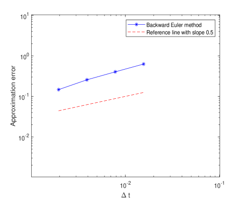
Figure 1: Convergence rate of BEM for (6.1)

In order to check the theory in Theorem 3.4, we perform a numerical experiment with four different stepsizes $\Delta=2^{-9}$, $2^{-8}$, $2^{-7}$, $2^{-6}$ at $T=1$. The numerical solution with stepsize $\Delta=2^{-11}$ is regarded as the exact solution of this experiment since it is difficult to be expressed explicitly. Then mean-square error can be estimated by computing the average of 500 sample paths’ errors between exact solutions and numerical solutions. Figure 1 illustrates the mean-square error which is defined by

$$(\mathbb{E}|x(T)-Z_{N}|^{2})^{\frac{1}{2}}\approx\left(\frac{1}{500}\sum_{i=1}^{500}|x^{i}(T)-Z^{i}_{N}|^{2}\right)^{\frac{1}{2}}.$$

From Figure 1, we can observe that the convergence rate of BEM is close to 0.5, which means that it is coincident with the theoretical conclusion in Theorem 3.4.

Example 2

Consider the following scalar nonlinear SDDE

$$dx(t)=\left(-2x(t)-4x(t)^{3}+x(t-\tau)\right)dt+\left(x(t)^{2}+\frac{1}{2}x(t-\tau)\right)dW(t),$$ (6.2)

on $t\geq 0$. Here, the initial data $\varphi(t)=|t|^{\frac{1}{2}}+3$, $t\in[-\tau,0]$. Let $l=2$, then we can see that

$$\langle x,\alpha(x,y)\rangle=x(-2x-4x^{3}+y)\leq-\frac{3}{2}|x|^{2}-4|x|^{4}+\frac{1}{2}|y|^{2},$$

$$|\beta(x,y)|^{2}=|x^{2}+\frac{1}{2}y|^{2}\leq 2|x|^{4}+\frac{1}{2}|y|^{2},$$

which means that the drift and diffusion coefficients satisfy Assumption 5.1.

Figure 2: Mean-square stability of BEM with $\Delta=0.001$

We compute the average of the numerical solutions simulated by 500 sample paths with stepsize $\Delta=0.001$ and plot its trajectory in Figure 2. From Figure 2, we can know that the trajectory tends to zero as time goes on, which means that the numerical solution of BEM is mean-square stable.

Funding

This work is supported by the National Natural Science Foundation of China (11871343) and Shanghai Rising-Star Program (22QA1406900).

Availability of data and materials

Not applicable.

Competing interests

The authors declare that they have no competing interests.

References

• [1] E. Allen, Modeling with Itô Stochastic Differential Equations, Springer, Dordrecht, 2007.
• [2] A.Andersson, R. Kruse, Mean-square convergence of the BDF2-Maruyama and backward Euler schemes for SDE satisfying a global monotonicity condition, BIT 57(1) (2017) 21-53.
• [3] D.F. Anderson, D.J. Higham, Y.Sun, Multilevel Monte Carlo for stochastic differential equations with small noise, SIAM J. Numer. Anal. 54(2) (2016) 505-529.
• [4] J.A.D. Appleby, M. Guzowska, C. Kelly, A. Rodkina, Preserving positivity in solutions of discretised stochastic differential equations, Appl. Math. Comput. 217(2) (2010) 763-774.
• [5] W. Beyn, E. Isaak, R. Kruse, Stochastic C-stability and B-consistency of explicit and implicit Euler-type schemes, J. Sci. Comput. 67(3) (2016) 955-987.
• [6] E. Buckwar, A. Pikovsky, M. Scheutzow, Stochastic dynamics with delay and memory-Preface, Stoch. Dyn. 5(2) (2005) III-IV.
• [7] W. Cao, P. Hao, Z. Zhang, Split-step $\theta$-method for stochastic delay differential equations, Appl. Numer. Math. 76 (2014) 19-33.
• [8] L. Chen, F. Wu, Almost sure exponential stability of the backward Euler–Maruyama scheme for stochastic delay differential equations with monotone-type condition, J. Comput. Appl. Math. 282 (2015) 44-53.
• [9] S. Deng, C. Fei, W. Fei, X. Mao, Tamed EM schemes for neutral stochastic differential delay equations with superlinear diffusion coefficients, J. Comput. Appl. Math. 388 (2021) 113269.
• [10] O. Farkhondeh Rouz, Preserving asymptotic mean-square stability of stochastic theta scheme for systems of stochastic delay differential equations, Comput. Methods Differ. Equ. 8(3) (2020) 468-479.
• [11] W. Fei, L. Hu, X. Mao, D. Xia, Advances in the truncated Euler-Maruyama method for stochastic differential delay equations, Commun. Pure Appl. Anal. 19(4) (2020) 2081-2100.
• [12] S. Gan, H. Schurz, H. Zhang, Mean square convergence of stochastic $\theta$-methods for nonlinear neutral stochastic differential delay equations, Int. J. Numer. Anal. Model. 8(2) (2011) 201-213.
• [13] Q. Guo, X. Mao, R. Yue, The truncated Euler–Maruyama method for stochastic differential delay equations, Numer. Algorithms, 78(2) (2018) 599-624.
• [14] D.J. Higham, Mean-square and asymptotic stability of stochastic theta method, SIAM J. Numer. Anal. 38 (2000) 753–769.
• [15] D.J. Higham, Stochastic ordinary differential equations in applied and computational mathematics, IMA J. Appl. Math. 76(3) (2011) 449-474.
• [16] D.J. Higham, X.Mao, C. Yuan, Almost sure and moment exponential stability in the numerical simulation of stochastic differential equations, SIAM J. Numer. Anal. 45 (2007) 592–609.
• [17] C. Huang, Mean square stability and dissipativity of two classes of theta methods for systems of stochastic delay differential equations, J. Comput. Appl. Math. 259 (2014) 77-86.
• [18] M. Hutzenthaler, A. Jentzen, P.E. Kloeden, Strong and weak divergence in finite time of Euler’s method for stochastic differential equations with non-globally Lipschitz continuous coefficients, Proc. R. Soc. A, Math. Phys. Eng. Sci. 467 (2011) 1563–1576.
• [19] M. Hutzenthaler, A. Jentzen, P.E. Kloeden, Strong convergence of an explicit numerical method for SDEs with nonglobally Lipschitz continuous coefficients, Ann. Appl. Probab. 22(4) (2012) 1611-1641.
• [20] P.E. Kloeden, E. Platen, Numerical Solution of Stochastic Differential Equations, Springer, Berlin, 1992.
• [21] G. N. Milstein, M. V. Tretyakov, Stochastic numerics for mathematical physics, Springer, Berlin, 2004.
• [22] M. Li, C. Huang, Projected Euler-Maruyama method for stochastic delay differential equations under a global monotonicity condition, Appl. Math. Comput. 366 (2020) 124733.
• [23] Q. Li, S. Gan, Almost sure exponential stability of numerical solutions for stochastic delay differential equations with jumps, J. Appl. Math. Comput. 37(1) (2011) 541-557.
• [24] X. Li, X. Mao, G. Yin, Explicit numerical approximations for stochastic differential equations in finite and infinite horizons: truncation methods, convergence in pth moment and stability, IMA J. Numer. Anal. 39 (2019) 847-892.
• [25] M. Liu, W. Cao, Z. Fan, Convergence and stability of the semi-implicit Euler method for a linear stochastic differential delay equation, J. Comput. Appl. Math. 170(2) (2004) 255-268.
• [26] W. Liu, X. Mao, Strong convergence of the stopped Euler–Maruyama method for nonlinear stochastic differential equations, Appl. Math. Comput. 223 (2013) 389-400.
• [27] W. Liu, X. Mao, Y. Wu, The backward Euler-Maruyama method for invariant measures of stochastic differential equations with super-linear coefficients, arXiv preprint arXiv:2206.09970, 2022.
• [28] X. Mao, Stochastic Differential Equations and Applications, 2nd ed. Horwood, Chichester, 2007.
• [29] X. Mao, The truncated Euler-Maruyama method for stochastic differential equations, J. Comput. Appl. Math. 290 (2015) 370-384.
• [30] X. Mao, L. Szpruch, Strong convergence and stability of implicit numerical methods for stochastic differential equations with non-globally Lipschitz continuous coefficients, J. Comput. Appl. Math. 238 (2013) 14-28.
• [31] X. Mao, L. Szpruch, Strong convergence rates for backward Euler–Maruyama method for non-linear dissipative-type stochastic differential equations with super-linear diffusion coefficients, Stochastics. 85(1 (2013) 144-171.
• [32] X. Mao, Y. Shen, A. Gray, Almost sure exponential stability of backward Euler–Maruyama discretizations for hybrid stochastic differential equations, J. Comput. Appl. Math. 235(5) (2011) 1213-1226.
• [33] M. Milošević, Convergence and almost sure exponential stability of implicit numerical methods for a class of highly nonlinear neutral stochastic differential equations with constant delay, J. Comput. Appl. Math. 280 (2015) 248-264.
• [34] M. Milošević, Implicit numerical methods for highly nonlinear neutral stochastic differential equations with time-dependent delay, Appl. Math. Comput. 244 (2014) 741-760.
• [35] H. Mo, F. Deng, C. Zhang, Exponential stability of the split-step $\theta$-method for neutral stochastic delay differential equations with jumps, Appl. Math. Comput. 315 (2017) 85-95.
• [36] H. Mo, L. Liu, M. Xing, F. Deng, B. Zhang, Exponential stability of implicit numerical solution for nonlinear neutral stochastic differential equations with time‐varying delay and poisson jumps, Math. Methods Appl. Sci.44(7) (2021) 5574-5592.
• [37] X. Qu, C. Huang, Delay-dependent exponential stability of the backward Euler method for nonlinear stochastic delay differential equations, Int. J. Comput. Math. 89(8) (2012) 1039-1050.
• [38] S. Sabanis, Euler approximations with varying coefficients: the case of superlinearly growing diffusion coefficients, Ann. Appl. Probab. 26(4) (2016) 2083-2105.
• [39] G. Song, J. Hu, S. Gao, X. Li , The strong convergence and stability of explicit approximations for nonlinear stochastic delay differential equations, Numer. Algorithms 89(2) (2022) 855-883.
• [40] L. Szpruch, X. Mao, D.J. Higham, J. Pan, Numerical simulation of a strongly nonlinear Ait-Sahalia-type interest rate model, BIT 51(2) (2011) 405-425.
• [41] L. Wang, C. Mei, H. Xue, The semi-implicit Euler method for stochastic differential delay equation with jumps, Appl. Math. Comput. 192(2) (2007) 567-578.
• [42] W. Wang, Y. Chen, Mean-square stability of semi-implicit Euler method for nonlinear neutral stochastic delay differential equations, Appl. Numer. Math. 61(5) (2011) 696-701.
• [43] X. Wang, S. Gan, The improved split-step backward Euler method for stochastic differential delay equations, Int. J. Comput. Math. 88(11) (2011) 2359-2378.
• [44] X. Wang, J. Wu, B. Dong , Mean-square convergence rates of stochastic theta methods for SDEs under a coupled monotonicity condition, BIT 60(3) (2020) 759-790.
• [45] F. Wu, X. Mao, L. Szpruch, Almost sure exponential stability of numerical solutions for stochastic delay differential equations, Numer. Math. 115(4) (2010) 681-697.
• [46] Z. Yan, A. Xiao, X. Tang, Strong convergence of the split-step theta method for neutral stochastic delay differential equations, Appl. Numer. Math. 120 (2017) 215-232.
• [47] Z. Yu, The improved stability analysis of the backward Euler method for neutral stochastic delay differential equations, Int. J. Comput. Math. 90(7) (2013) 1489-1494.
• [48] C. Yue, L. Zhao, Strong convergence of the split-step backward Euler method for stochastic delay differential equations with a nonlinear diffusion coefficient, J. Comput. Appl. Math. 382 (2021) 113087.
• [49] C. Zhang, Y. Xie, Backward Euler-Maruyama method applied to nonlinear hybrid stochastic differential equations with time-variable delay, Sci. China Math. 62(3) (2019) 597-616.
• [50] H. Zhang, S. Gan, L. Hu, The split-step backward Euler method for linear stochastic delay differential equations, J. Comput. Appl. Math. 225(2) (2009) 558-568.
• [51] G. Zhao, M. Liu, Numerical methods for nonlinear stochastic delay differential equations with jumps,Appl. Math. Comput. 233 (2014) 222-231.
• [52] S. Zhou, Strong convergence and stability of backward Euler–Maruyama scheme for highly nonlinear hybrid stochastic differential delay equation, Calcolo 52(4) (2015) 445-473.
• [53] S. Zhou, H. Jin, Numerical solution to highly nonlinear neutral-type stochastic differential equation, Appl. Numer. Math. 140 (2019) 48-75.
• [54] X. Zong, F. Wu, Exponential stability of the exact and numerical solutions for neutral stochastic delay differential equations,Appl. Math. Model. 40(1) (2016) 19-30.
• [55] X. Zong, F. Wu, C. Huang, Theta schemes for SDDEs with non-globally Lipschitz continuous coefficients, J. Comput. Appl. Math. 278 (2015) 258-277.