Sharp $\ell^{p}$ inequalities for discrete singular integrals

Abstract.

This paper constructs a collection of discrete operators on the $d$-dimensional lattice $\mathbb{Z}^{d}$, $d\geq 1$, which result from the conditional expectation of martingale transform in the upper half-space $\mathbb{R}^{d+1}_{+}$ constructed from Doob $h$-processes. Special cases of these operators are what we call the probabilistic discrete Riesz transforms. When $d=1,$ they reduce to the probabilistic discrete Hilbert transform used by the first and third authors to resolve the long-standing open problem concerning the $\ell^{p}$ norm, $1<p<\infty$, of the discrete Hilbert transform on the integers $\mathbb{Z}$. The construction for $d>1$ is motivated by a similar problem, Conjecture 5.5, concerning the norm of the discrete Riesz transforms arising from discretizing singular integrals on $\mathbb{R}^{d}$ as in the original paper of A. P. Calderón and A. Zygmund, and subsequent works of A. Magyar, E. M. Stein, S. Wainger, L. B. Pierce and many others, concerning operator norms in discrete harmonic analysis. For any $d\geq 1$, it is shown that the probabilistic discrete Riesz transforms have the same $\ell^{p}$ norm as the continuous Riesz transforms on $\mathbb{R}^{d}$ which is dimension independent and equals the norm of the classical Hilbert transform on $\mathbb{R}$. Along the way we give a different proof, based on Fourier transform techniques, of the key estimate used to identify the norm of the discrete Hilbert transform.

1. Introduction

The probabilistic representation à la Gundy–Varopoulos [GV79] of the classical Riesz transforms and other singular integrals and Fourier multipliers as conditional expectations (projections) of stochastic integrals, in combination with the sharp martingale inequalities of Burkholder [Bur84] and their versions for orthogonal martingales [BanWang] and non-symmetric transforms [Choi, BanOse1], have proven to be powerful tools in obtaining sharp, or near sharp, $L^{p}$-bounds for these operators in a variety of geometric settings. A particular feature of these techniques is that they give $L^{p}$-bounds independent of the geometry of the ambient space, including dimension. For example, such representation was used to show that the $L^{p}$-norm, $1<p<\infty$, of the Riesz transforms on $\mathbb{R}^{d}$, $d>1$, is the same as that of the Hilbert transform on $\mathbb{R}$ found by S. Pichorides [Pic72] and to obtain the first explicit bounds for the Beurling–Ahlfors transform, see [BanWang]. The former was first proved using the method of rotations in [IwaMar]. For some history on norm estimates for the Beurling–Ahlfors transform motivated by the celebrated 1982 conjecture of T. Iwaniec [Iwa82], and the current best known bound, see [BanJan].

One advantage of the martingale approach in obtaining explicit bounds is that it immediately extends to geometric and analytic settings well beyond $\mathbb{R}^{d}$, including Wiener space, quite general semigroups including those of Lévy processes and discrete Laplacian on groups. The interest on dimension free estimates for Riesz transforms and other operators in harmonic analysis was sparked by the results and questions raised in Stein [SteSome] and Meyer [Mey1]. For some of the now vast literature on dimension free, and sharp bounds, for Riesz transforms and Fourier multipliers in a variety of geometric and analytic settings, we refer the reader to [Ban, BanBog, BBL20, BO15, BO18, OY21, GesMonSak, BanMen, Gun89, BBLS2021, CarSam, Tor, ADP20, Pet2, Pet3, BanOse1, LiX, NazVol, Ose2, Lus-Piq3, Lus-Piq4, Nao, Pis, DraVol1, DraVol2, DraVol3, DraVol4, CarDra1, CarDra2, Bak1] and references contained therein.

In his celebrated 1928 paper [Riesz], M. Riesz solved a problem of considerable interest at the time by showing that the Hilbert transform

(1.1) $$Hf(x)=p.v.\frac{1}{\pi}\int_{\mathbb{R}}\frac{f(x-y)}{y}dy,\quad f\in L^{p}(\mathbb{R}),$$

is a bounded operator on $L^{p}(\mathbb{R})$, $1<p<\infty$. For some history of this problem and Riesz’s solution in 1925 before its publication in 1928, we refer the reader to M. Cartwright’s article “Manuscripts of Hardy, Littlewood, Marcel Riesz and Titchmarsh,” [Car1982]. In his paper Riesz also showed that the boundedness of $H$ on $L^{p}(\mathbb{R})$ implies the boundedness of the discrete version $H_{\mathrm{dis}}$ on $\ell^{p}(\mathbb{Z})$, where the latter is defined by

(1.2) $$H_{\mathrm{dis}}f(n)=\frac{1}{\pi}\sum_{m\in\mathbb{Z}\setminus\{0\}}\frac{f(n-m)}{m},\quad f\in\ell^{p}(\mathbb{Z}).$$

In fact, Riesz showed that the operator norms satisfy

(1.3) $$\|H\|_{L^{p}\to L^{p}}\leq\|H_{\mathrm{dis}}\|_{\ell^{p}\to\ell^{p}},\quad\|H_{\mathrm{dis}}\|_{\ell^{p}\to\ell^{p}}\leq C\|H\|_{L^{p}\to L^{p}},$$

where $C$ is a constant independent of $p$.

The discrete Hilbert transform was introduced by D. Hilbert in 1909 who also verified its boundedness on $\ell^{2}(\mathbb{Z})$. Proving that the operator norms of $H$ and $H_{\mathrm{dis}}$, $1<p<\infty$, are the same has been a long-standing open problem motivated in part by an erroneous proof of E. C. Titchmarsh in 1926, [Titc26, Titc27]. In [Pic72], S. Pichorides showed that $\|H\|_{L^{p}\to L^{p}}=\cot(\pi/(2p^{*}))$, where $p^{*}=\max(p,p/(p-1))$. In [Laeng], the same is shown for $H_{\mathrm{dis}}$ when $p$ is of the form $2^{k}$ or ${2^{k}/(2^{k}-1)}$, $k=1,2,\dots$ The proof is attributed to I. Verbitsky. For further history and references related to this problem, see [Laeng, HarLitPol, CarSam, Tor, ADP20, Pet2, Pet3]. In [BanKwa], the equality of the norms was proved for all $1<p<\infty$ by extending the Gundy–Varopoulos construction for Riesz transforms to martingale transforms of Doob $h$-processes where the harmonic function $h$ corresponds to the periodic Poisson kernel. It was shown there that the discrete Hilbert transform arises as the convolution of the projection of one of these Doob martingale transforms, which has the desired bound, with a probability kernel. Hence although this more general construction à la Gundy–Varopoulos does not lead to an exact representation of the discrete Hilbert transform, unlike the situation of the continuous version of the Hilbert transform and the Riesz transforms on $\mathbb{R}^{d}$, the extra step of convolving with a probability kernel preserves the norm and resolves the equality of the norms of $H$ and $H_{{\mathrm{dis}}}$ for all $1<p<\infty$.

Given the successful use of the probabilistic techniques in deriving sharp and dimension free estimates for singular integrals and Fourier multipliers as discussed above, and the interest on discrete analogues of many classical operators in harmonic analysis as studied in [MSW, Pie1, Pie2, Pie3, Pie4, Pie5, Pierce, SW2000, SteWai99] (and many other references contained therein), the following questions naturally arise.

Question 1.1.

Can the construction of the probabilisitic operators in [BanKwa] be carried out in higher dimension to obtain a collection of operators on $\mathbb{Z}^{d}$, $d>1$, which are closely related to the Riesz transforms and that have $\ell^{p}(\mathbb{Z}^{d})$-norms independent of $d$? Are the extension of these operators to $\mathbb{R}^{d}$ obtained simply by replacing the discrete variable $n\in\mathbb{Z}^{d}$ by the continuous variable $z\in\mathbb{R}^{d}$ in their kernels with the appropriate modification for the singularity at $z=0$, also bounded on $L^{p}(\mathbb{R}^{d})$? Are they Calderón–Zygmund operators?

Question 1.2.

Is it possible to extend the sharp result in [BanKwa] for the discrete Hilbert transform in $\mathbb{Z}$ to the case of the discrete Riesz transforms in $\mathbb{Z}^{d}$ where the latter are defined as discrete convolutions with the corresponding Calderón–Zygmund kernels, i.e., as defined in the classical paper of Calderón and Zygmund [CZ, pg. 138]? The precise formulation of this question, which we state as a conjecture, is found in Section 5.2.

In this paper we show that there is a natural collection of discrete operators on $\mathbb{Z}^{d}$ which have norms independent of the dimension and with the same constants as those in the martingale transform inequalities of [Bur84] and [BanWang]. From these operators we define what we call the probabilistic discrete Riesz transforms, denoted by $T_{\mathbb{H}^{(k)}}$, $k=1,2,\dots,d$, and show that for all $d$ and all $k$,

(1.4) $$\|T_{\mathbb{H}^{(k)}}\|_{\ell^{p}\to\ell^{p}}=\cot(\pi/(2p^{*})),\quad 1<p<\infty.$$

These operators are closely related to the discrete Calderón–Zygmund Riesz transforms. When $d=1$, they reduce to what we call the probabilistic discrete Hilbert transform, denoted by $T_{\mathbb{H}}$, for which, with the additional step that $H_{\mathrm{dis}}$ is the convolution of $T_{\mathbb{H}}$ with a probability kernel, gives

(1.5) $$\|T_{\mathbb{H}}\|_{\ell^{p}{\to\ell^{p}}}=\|H_{\mathrm{dis}}\|_{\ell^{p}\to\ell^{p}}=\|H\|_{L^{p}\to L^{p}}=\cot\left(\frac{\pi}{2p^{*}}\right),\quad 1<p<\infty.$$

2. Organization and summary of results

The paper is organized as follows.

• Section 3.1 introduces the periodic Poisson kernel $h$ on $\mathbb{R}^{d}$, $d\geq 1$, from which we will define the Doob $h$-process used throughout the paper and derives some of its basic properties. An important difference between $d=1$ and $d>1$ is that in the first case we can write a simple explicit expression for $h$ from which many explicit computations are possible. A similar formula is not available for $d>1$.

• Section 3.2 defines the $h$-harmonic extension of the function $f:\mathbb{Z}^{d}\to\mathbb{R}$ and discusses a connection to an interesting open problem of Magyar, Stein, and Wainger in  [MSW], see Remark 3.5.

• Section 3.3 defines the Doob $h$-process associated with the function $h$, their martingale transforms and recalls the relevant martingale inequalities.

• Section 4.1 defines the projection operators, denoted by $T_{A}$, as the conditional expectations of the martingale transforms. Theorems 4.1 and 4.4 compute their kernels and prove their boundedness on $\ell^{p}(\mathbb{Z}^{d})$ with the same constants as those in the martingale inequalities.

• Section 5.1 considers the discrete Calderón–Zygmund operators given by (5.4) and proves their boundedness properties, see Propositions 5.1 and 5.2. Conjecture 5.5, and the weaker Problem 5.6, on the norm of the discrete Riesz transforms à la Calderón–Zygmund are formulated in this section.

• Section 6.1 defines the probabilistic discrete Riesz transforms on $\mathbb{Z}^{d}$ and shows that their $\ell^{p}(\mathbb{Z}^{d})$-norms are the same as the norms of the classical Riesz transforms on $L^{p}(\mathbb{R}^{d})$, $1<p<\infty$, see Theorem 6.6. From this it follows that the $p$-norms of the classical Riesz transforms on $L^{p}(\mathbb{R}^{d})$, the classical Hilbert transform on $L^{p}(\mathbb{R})$, the discrete Hilbert transform on $\ell^{p}(\mathbb{Z})$, and probabilistic discrete Riesz transforms on $\ell^{p}(\mathbb{Z}^{d})$ are all equal to $\cot(\pi/(2p^{*}))$. This gives further evidence of the validity of Conjecture 5.5.

• Section 7 computes the Fourier transform of the probabilistic discrete Hilbert transform. This allows for a new proof of the key Lemma 1.3 in [BanKwa] which shows that the discrete Hilbert transform $H_{\mathrm{dis}}$ is the convolution of the probabilistic discrete Hilbert transform with a probability kernel, see Theorem 7.1. The proof here, based on the Fourier transform and Bochner’s theorem on positive-definite functions (Lemma 7.6), is computationally much simpler than the one given in [BanKwa]. From this, the sharp $\ell^{p}$-bound for $H_{\mathrm{dis}}$ follows. The natural question for $\mathbb{Z}^{d}$, $d\geq 2$, is stated at the end of this section, see Question 7.7.

• Section 8 shows that replacing the discrete variable $n\in\mathbb{Z}^{d}$ by the continuous variable $z\in\mathbb{R}^{d}$ in the kernel for the probabilistic discrete Riesz transforms, and after a modification which does not affect the discrete operator, gives operators that are bounded on $L^{p}(\mathbb{R}^{d})$, $1<p<\infty$, and except for discontinuity on the sphere they satisfy (5.3) in the definition of Calderón–Zygmund kernels, see Theorem 8.1 and Corollaries 8.3 and 8.4.

• Section 9 discusses a “method of rotation” by constructing certain discrete Riesz transforms on $\mathbb{Z}^{d}$ motivated by the classical ones and verifying that these Riesz transforms have the same norms as the discrete Hilbert transform $H_{\mathrm{dis}}$ and the probabilistic discrete Riesz transforms $T_{\mathbb{H}^{(k)}}$, see Theorem 9.5. This section ends with Theorem 9.6 summarizing the $\ell^{p}$-norms for the various discrete versions of Hilbert and Riesz transforms studied in this paper.

• Section 10 presents some numerical calculations comparing the relative sizes of the kernels for the discrete Riesz transforms, the probabilistic discrete Riesz transforms and the discrete Riesz transforms constructed in the method of rotations.

Notation

The Fourier transform of a function $f$ on $\mathbb{R}^{d}$ is denoted by $\widehat{f}$, where

$$\widehat{f}(\xi)=\int_{\mathbb{R}^{d}}f(x)e^{-2\pi ix\cdot\xi}d\xi\quad\text{for }x\in\mathbb{R}^{d}.$$

For a function $f:\mathbb{Z}^{d}\to\mathbb{R}$, the Fourier transform is denoted by $\mathcal{F}(f)$, where

$$\mathcal{F}(f)(\xi)=\sum_{n\in\mathbb{Z}^{d}}f(n)e^{-2\pi in\cdot\xi}\quad\text{for }\xi\in Q:=[-\tfrac{1}{2},\tfrac{1}{2})^{d}.$$

Here, $Q$ is often called the fundamental cube.

The standard notations $\|f\|_{L^{p}}$ and $\|f\|_{\ell^{p}}$ are used for the $p$-norm of functions in $L^{p}(\mathbb{R}^{d})$ and $\ell^{p}(\mathbb{Z}^{d})$, respectively. $\|T\|_{L^{p}\to L^{p}}$ will denote the operator norm of $T:L^{p}(\mathbb{R}^{d})\to L^{p}(\mathbb{R}^{d})$, and similarly $\|T\|_{\ell^{p}\to\ell^{p}}$ for the operator norm of $T:\ell^{p}(\mathbb{Z}^{d})\to\ell^{p}(\mathbb{Z}^{d})$.

The gradient and Laplacian of functions $u(x,y)$ on the upper half-space $\mathbb{R}^{d}\times\mathbb{R}_{+}=\{(x,y):x\in\mathbb{R}^{d},y>0\}$ are denoted by

$$\nabla u=\left(\frac{\partial u}{\partial x_{1}},\cdots,\frac{\partial u}{\partial x_{d}},\frac{\partial u}{\partial y}\right)=\left(\nabla_{x}u,\,\,\frac{\partial u}{\partial y}\right)$$

and

$$\Delta u=\sum_{i=1}^{d}\frac{\partial^{2}u}{\partial x{{}_{i}}^{2}}+\frac{\partial^{2}u}{\partial y^{2}}=\Delta_{x}u+\frac{\partial u^{2}}{\partial y^{2}},$$

respectively. By abuse of notation, for $f:\mathbb{R}^{d}\to\mathbb{R}$ we will still use $\Delta f=\sum_{i=1}^{d}\frac{\partial^{2}f}{\partial x{{}_{i}}^{2}}$ to denote its Laplacian on $\mathbb{R}^{d}$.

Throughout the paper,

$$p^{*}=\max{\biggl{\{}}p,\frac{p}{p-1}{\biggr{\}}},\quad 1<p<\infty.$$

$C,C_{1},C_{2},\dots,C_{d}$ will denote constants that depend only on $d$ and whose value may change from line to line.

3. Preliminaries

3.1. The periodic Poisson kernel

Let $d\geq 1$. The Poisson kernel for the upper half-space $\mathbb{R}^{d}\times\mathbb{R}_{+}$ is given by

(3.1) $$p(x,y)=\frac{c_{d}y}{(|x|^{2}+y^{2})^{\frac{d+1}{2}}},\quad(x,y)\in\mathbb{R}^{d}\times\mathbb{R}_{+},\quad c_{d}=\Gamma{\biggl{(}}\frac{d+1}{2}{\biggr{)}}\pi^{-\frac{d+1}{2}}.$$

For $x,z\in\mathbb{R}^{d}$ and $y\in\mathbb{R}_{+}$, we set $p_{z}(x,y)=p(x-z,y)$. Since $\Delta p_{z}(x,y)=0$ and $p_{z}(x,y)>0$ for all $(x,y)\in\mathbb{R}^{d}\times\mathbb{R}_{+}$ and $z\in\mathbb{R}^{d}$, we see that the function $h$ defined by

(3.2) $$h(x,y)=\sum_{n\in\mathbb{Z}^{d}}p_{n}(x,y)$$

is also positive and harmonic. In addition, it is periodic in $x$ in a sense that $h(x+m,y)=h(x,y)$ for all $m\in\mathbb{Z}^{d}$. We call the function $h(x,y)$ the periodic Poisson kernel. The following properties of $h(x,y)$ will be used frequently in the sequel.

Lemma 3.1.

We have $\lim_{y\to\infty}h(x,y)=1$ uniformly in $x\in\mathbb{R}^{d}$. In particular, for each $y_{0}>0$, there exist constants $C_{1},C_{2}>0$ such that $C_{1}\leq h(x,y)\leq C_{2}$, for all $x\in\mathbb{R}^{d}$ and $y\geq y_{0}$.

Proof.

Recall that $Q={[-\frac{1}{2},\frac{1}{2})^{d}}.$ For $x\in\mathbb{R}^{d}$ and $y>0$, we have

$$1=\int_{\mathbb{R}^{d}}p(x-z,y)\,dz=\sum_{n\in\mathbb{Z}^{d}}\int_{n+Q}p(x-z,y)\,dz=\sum_{n\in\mathbb{Z}^{d}}\int_{Q}p_{n}(x-z,y)\,dz.$$

We will estimate the quantity

$$p_{n}(x,y)-\int_{Q}p_{n}(x-z,y)\,dz=\int_{Q}(p_{n}(x,y)-p_{n}(x-z,y))\,dz.$$

All constants $C_{1},C_{2},\ldots$ below are positive and depend only on $d$. Observe that we have

$$|\nabla_{x}p(x,y)|\leq C_{1}\frac{y}{(|x|^{2}+y^{2})^{\frac{d}{2}+1}}$$

for all $(x,y)\in\mathbb{R}^{d}\times\mathbb{R}_{+}$. Furthermore, if $x\in\mathbb{R}^{d}$, $y\geq 1$, $z\in Q$ and $n\in\mathbb{Z}^{d}$, then

$$|x-n-z|^{2}+y^{2}\geq C_{2}|x-n|^{2}+y^{2}.$$

It follows that

$$|\nabla_{x}p_{n}(x-z,y)| \leq C_{1}\,\frac{y}{(|x-n-z|^{2}+y^{2})^{\frac{d}{2}+1}}$$

$$\leq C_{3}\,\frac{y}{(|x-n|^{2}+y^{2})^{\frac{d}{2}+1}}$$

$$\leq C_{4}\,\frac{p_{n}(x,y)}{(|x-n|^{2}+y^{2})^{\frac{1}{2}}}\leq C_{4}\,\frac{p_{n}(x,y)}{y}\,.$$

Thus,

$$|p_{n}(x,y)dz-p_{n}(x-z,y)|\leq C_{4}\,\frac{p_{n}(x,y)}{y}\times|z|\leq C_{5}\,\frac{p_{n}(x,y)}{y}.$$

We conclude that

$$|h(x,y)-1| =\left|\sum_{n\in\mathbb{Z}^{d}}\int_{Q}(p_{n}(x,y)dz-p_{n}(x-z,y))dz\right|$$

$$\leq\sum_{n\in\mathbb{Z}^{d}}\int_{Q}|p_{n}(x,y)dz-p_{n}(x-z,y)|dz$$

$$\leq\sum_{n\in\mathbb{Z}^{d}}\int_{Q}C_{5}\,\frac{p_{n}(x,y)}{y}\,dz=\frac{C_{5}}{y}\,.$$

This proves the first statement of the lemma. The second assertion (ii) follows from (i) and the fact that $h(x,y)$ is positive, continuous, and periodic in $x$. ∎

Clearly, $h(x,y)\geq p(x,y)$, and thus for some constant $C_{1}$ depending only on $d$ we have $h(x,y)\geq C_{1}y$ whenever $x\in Q$ and $y\in(0,1)$. Since $h(x,y)$ is periodic in $x$ with period $1$, the same estimate holds for all $x\in\mathbb{R}^{d}$, and by combining this inequality with Lemma 3.1, we find that

(3.3) $$h(x,y)\geq C_{2}\min\{1,y\}$$

for all $(x,y)\in\mathbb{R}^{d}\times\mathbb{R}_{+}$. Similarly, we have $h(x,y)\geq p(x,y)\geq C_{3}\frac{y}{\sqrt{x^{2}+y^{2}}}$ when $x^{2}+y^{2}<1$ and $y\in(0,1)$. For all other $(x,y)$ the last estimate is weaker than (3.3) (up to a constant factor), so we conclude that

(3.4) $$h(x,y)\geq C_{4}\,\frac{y}{\sqrt{x^{2}+y^{2}}}$$

holds for all $(x,y)\in\mathbb{R}^{d}\times\mathbb{R}_{+}$.

We recall the Poisson summation formula.

Proposition 3.2 ([Graf]*Theorem 3.1.17).

Suppose that $f,\widehat{f}\in L^{1}(\mathbb{R}^{d})$ and

$$|f(x)|+|\widehat{f}(x)|\leq C(1+|x|)^{-n-\delta}$$

for some $C,\delta>0$. Then $f$ and $\widehat{f}$ are continuous and

(3.5) $$\sum_{n\in\mathbb{Z}^{d}}f(x+n)=\sum_{n\in\mathbb{Z}^{d}}\widehat{f}(n)e^{2\pi in\cdot x}$$

for all $x\in\mathbb{R}^{d}$.

Applying to the function $f(x)=p(x,y)$ for which $\widehat{f}(n)=e^{-2\pi|n|y}$, we obtain that

(3.6) $$h(x,y)=\sum_{n\in\mathbb{Z}^{d}}p_{0}(x+n,y)=\sum_{n\in\mathbb{Z}^{d}}e^{-2\pi|n|y}e^{2\pi in\cdot x}.$$

From the fact that the Poisson kernel for the unit disc $\mathcal{P}_{r}(\theta)$ is given by

$$\mathcal{P}_{r}(\theta)=\sum_{n\in\mathbb{Z}}r^{|n|}e^{in\theta}=\frac{1-r^{2}}{1+r^{2}-2r\cos\theta},\quad 0\leq r\leq 1,\quad 0\leq\theta\leq 2\pi,$$

we see that for $d=1$,

(3.7) $$h(x,y)=\frac{1}{2\pi}\mathcal{P}_{e^{-2\pi y}}(2\pi x)=\frac{\sinh(2\pi y)}{\cosh(2\pi y)-\cos(2\pi x)}.$$

This explicit expression for $h$ when $d=1$ is well known, see for example [IwaKow]*pg.70. It was derived in [BanKwa]*Lemma 3.1 by a different argument and used there for many calculations. In particular, for $d=1$, such formula permits explicit calculations for various quantities involving the function $\frac{1}{h(x,y)}$, see [BanKwa]. In Section 7 we will use this in the calculation of the Fourier transform of the kernel $K_{\mathbb{H}}$ for the probabilistic discrete Hilbert transform. For $d\geq 2$, while we can express $h(x,y)$ in various other forms besides (3.2) and (3.6), it does not seem possible to write such a convenient closed formula that will facilitate calculations with $\frac{1}{h(x,y)}$ in a similar manner.

3.2. $h$-harmonic extension

Let $f:\mathbb{Z}^{d}\to\mathbb{R}$ be a function of compact support, that is, $f(n)=0$ all but finitely many $n\in\mathbb{Z}^{d}$. Define

(3.8) $$u_{f}(x,y)=\sum_{n\in\mathbb{Z}^{d}}f(n)\frac{p_{n}(x,y)}{h(x,y)}.$$

Note that $u_{f}$ is $h$-harmonic. That is, $\Delta(hu_{f})=0$. Equivalently, $u_{f}(x,y)$ is harmonic in the upper half-space relative to the operator

$$\frac{1}{2}\Delta+\frac{\nabla h(x,y)\cdot\nabla}{h(x,y)}.$$

The following proposition provides information on the boundary values of $u_{f}$.

Proposition 3.3.

For each $x\in\mathbb{R}^{d}$, $p_{n}(x,y)/h(x,y)$ converges as $y\to 0$. Let $\Psi(x)$ be the limit, and $f\in\ell^{p}(\mathbb{Z}^{d})$ be compactly supported. Define $f_{\mathrm{ext}}(x):=\sum_{n\in\mathbb{Z}^{d}}f(n)\Psi(x-n)$. Then, $f_{\mathrm{ext}}(n)=f(n)$ for all $n\in\mathbb{Z}^{d}$ and $\|f_{\mathrm{ext}}\|_{L^{p}}\leq\|f\|_{\ell^{p}}$.

Proof.

Suppose $x=0$. Note that $p_{n}(0,y)/h(0,y)\leq 1$ and

$$h(0,y) =p(0,y)+\sum_{n\neq 0}p(n,y)=p(0,y)+\sum_{n\neq 0}\frac{c_{d}y}{\left(|n|^{2}+y^{2}\right)^{\frac{d+1)}{2}}}$$

$$\leq p(0,y)+c_{d}y\sum_{n\neq 0}|n|^{-(d+1)}.$$

Since the sum on the left hand side is finite, we have

$$\frac{1}{1+C_{d}y^{d+1}}\leq\frac{p(0,y)}{h(0,y)}\leq 1.$$

Thus, if $x=0$, the limit exists and $\Psi(0)=1$.

Suppose $x=n\in\mathbb{Z}^{d}\setminus\{0\}$. Then, $\lim_{y\to 0}p(n,y)=0$ and

$$\frac{1}{h(n,y)}\leq\frac{1}{p(0,y)}=\frac{1}{c_{d}}y^{d}\to 0.$$

Thus, the limit exists and $\Psi(n)=0$. For $x\in\mathbb{R}^{d}\setminus\mathbb{Z}^{d}$, we have $\lim_{y\to 0}p(x,y)/y=c_{d}|x|^{-d-1}$ and

$$\lim_{y\to 0}\frac{h(x,y)}{y}=c_{d}\sum_{n\in\mathbb{Z}^{d}}|x-n|^{-(d+1)}.$$

Since the sum is finite for each $x\in\mathbb{R}^{d}\setminus\mathbb{Z}^{d}$, we conclude that $\Psi(x)$ is well-defined. Note that

$$\int_{\mathbb{R}^{d}}\frac{p(x,y)}{h(x,y)}\,dx=\sum_{n\in\mathbb{Z}^{d}}\int_{Q}\frac{p_{n}(x,y)}{h(x,y)}\,dx=1$$

and

$$\sum_{n\in\mathbb{Z}^{d}}\frac{p(x-n,y)}{h(x-n,y)}=\sum_{n\in\mathbb{Z}^{d}}\frac{p_{n}(x,y)}{h(x,y)}=1.$$

By Fatou’s lemma, we have

$$\int_{\mathbb{R}^{d}}\Psi(x)\,dx\leq 1,\qquad\sum_{n\in\mathbb{Z}^{d}}\Psi(x-n)\leq 1.$$

Thus, it follows from Hölder’s inequality that

$$\|f_{\mathrm{ext}}\|_{L^{p}}^{p}=\int_{\mathbb{R}^{d}}|f_{\mathrm{ext}}(x)|^{p}\,dx\leq\left(\sum_{n\in\mathbb{Z}^{d}}|f(n)|^{p}\int_{\mathbb{R}^{d}}\Psi(x-n)\,dx\right)\left(\sum_{n\in\mathbb{Z}^{d}}\Psi(x-n)\right)^{p-1}\leq\|f\|_{\ell^{p}}^{p}.$$

∎

Remark 3.4.

Due to this Proposition, we call $u_{f}$ the discrete harmonic extension of $f$.

When $d=1$, we can use (3.7) to compute that

$${\Psi_{1}(x):=}\Psi(x)=\begin{cases}\frac{\sin^{2}(\pi x)}{\pi^{2}x^{2}},&x\neq 0,\\ 1,&x=0.\end{cases}$$

For an arbitrary $d=1,2,\dots$, set $\Psi_{d}(x)=\prod_{i=1}^{d}{\Psi_{1}}(x_{i})$ and consider the function

$$\widetilde{f}_{\mathrm{ext}}(x)=\sum_{n\in\mathbb{Z}^{d}}f(n)\Psi_{d}(x-n).$$

It was proved in [MSW] that for all $d\geq 1$, there exists a dimensional constant $A_{d}\geq 1$ such that

(3.9) $$\frac{1}{A_{d}}\|f\|_{\ell^{p}}\leq\|\widetilde{f}_{\mathrm{ext}}\|_{L^{p}}\leq A_{d}\|f\|_{\ell^{p}}.$$

The compact support of the Fourier transform of $\Psi_{d}(x)$, which we are not able to verify in our case for $\Psi(x)$ when $d>1$, is crucial for the first inequality in (3.9). The bounds in (3.9) were used in [MSW]*Proposition 2.1 to show that the $L^{p}$-norm of a continuous Fourier multiplier operator $T$, when the multiplier is bounded and of compact support, controls the $\ell^{p}$-norm of its discrete version $T_{\mathrm{dis}}$ with a constant depending on $d$. More precisely, suppose

$$\widehat{K}(\xi)=\int_{\mathbb{R}^{d}}K(x)e^{-2\pi ix\cdot\xi}dx$$

is bounded and supported on the fundamental cube $Q={[-\frac{1}{2},\frac{1}{2})^{d}}$. Define the Fourier multiplier $\widehat{Tf}(\xi)=\widehat{K}(\xi)\widehat{f}(\xi)$ and its discrete version by

$$T_{\mathrm{dis}}f(n)=\sum_{m\in\mathbb{Z}^{d}}K(m)f(n-m).$$

Fix $1\leq p\leq\infty$. If $T$ is bounded on $L^{p}(\mathbb{R}^{d})$, then $T_{\mathrm{dis}}$ is bounded on $\ell^{p}(\mathbb{Z}^{d})$ and

(3.10) $$\|T_{\mathrm{dis}}\|_{\ell^{p}\to\ell^{p}}\leq C_{d}\|T\|_{L^{p}\to L^{p}},$$

where $C_{d}=3^{d}A_{d}^{2}$.

Remark 3.5.

The problem raised in [MSW]*Remark (1), pg. 193,

“it would be interesting to know if $C_{d}$ can be taken to be independent of $d$, or for that matter if $C_{d}=1$,”

remains open to the best of knowledge, including the part concerning the independence of $d$.

3.3. The Doob $h$-process and martingale transforms

For the function $h(x,y)$ defined in (3.2), let $Z_{t}$ be a solution of the stochastic differential equation

$$dZ_{t}=dB_{t}+\frac{\nabla h(Z_{t})}{h(Z_{t})}dt,$$

where $(B_{t})_{t\geq 0}$ is the $(d+1)$-dimensional Brownian motion starting from $(x_{0},y_{0})\in\mathbb{R}^{d}\times\mathbb{R}_{+}$. The lifetime of $Z_{t}$ in the upper half-space is defined by $\tau=\inf\{t\geq 0:Y_{t}=0\}$. The lifetime $\tau$ is finite with probability one and the process $Z_{t}$ only exits the upper half-space on $\mathbb{Z}^{d}\times\{0\}$. Indeed, at its lifetime $Z_{t}$ approaches the point $n\in Z^{d}$ with probability $\frac{p_{n}(x,y)}{h(x,y)}$, where $(x,y)$ is the starting point of $Z_{t}$. For the basic properties and stochastic calculus for the Doob $h$-processes we refer the reader to [Bass, Chapter 3].

We denote by $\ell^{p}_{c}(\mathbb{Z}^{d})$ the space of all compactly supported functions in $\ell^{p}(\mathbb{Z}^{d})$. For $f\in\ell^{p}_{c}(\mathbb{Z}^{d})$, we define

$$M_{t}=M^{f}_{t}=u_{f}(Z_{t}),\quad\text{ for }t\in(0,\tau).$$

By Itô’s formula, $M^{f}_{t}$ is a martingale and satisfies

(3.11) $$M^{f}_{t} =M^{f}_{0}+\int_{0}^{t}\nabla u_{f}(Z_{s})\cdot dZ_{s}+\frac{1}{2}\int_{0}^{t}\Delta u_{f}(Z_{s})\,ds$$

$$=M^{f}_{0}+\int_{0}^{t}\nabla u_{f}(Z_{s})\cdot dZ_{s}-\int_{0}^{t}\frac{\nabla h(Z_{s})\cdot\nabla u_{f}(Z_{s})}{h(Z_{s})}\,ds$$

$$=M^{f}_{0}+\int_{0}^{t}\nabla u_{f}(Z_{s})\cdot dB_{s},$$

where $(B_{t})_{t\geq 0}$ is the $(d+1)$-dimensional Brownian motion.

Let $\mathfrak{M}_{(d+1)}(\mathbb{R})$ be the space of all $(d+1)\times(d+1)$ real matrices and denote its norm by

$$\|A\|=\sup\{\|Av\|:v\in\mathbb{R}^{d+1},\|v\|\leq 1\}.$$

By abuse of notation, for a matrix-valued function $A:\mathbb{R}^{d}\times\mathbb{R}_{+}\to\mathfrak{M}_{(d+1)}(\mathbb{R})$, that is, $A(x,y)=(A_{ij}(x,y))_{1\leq i,j\leq d+1}$ for all $x\in\mathbb{R}^{d}$ and $y>0$, we define

$$\|A\|=\sup_{(x,y)\in\mathbb{R}^{d}\times\mathbb{R}_{+}}\|A(x,y)\|=\sup\{\|A(x,y)v\|:v\in\mathbb{R}^{d+1},\|v\|\leq 1,(x,y)\in\mathbb{R}^{d}\times\mathbb{R}_{+}\}.$$

We say a matrix $A(x,y)=(A_{ij}(x,y))\in\mathfrak{M}_{(d+1)}(\mathbb{R})$ is orthogonal if $\langle A(x,y)v,v\rangle=\sum_{ij}A_{ij}v_{i}v_{j}=0$ for all $(x,y)\in\mathbb{R}^{d}\times\mathbb{R}_{+}$ and all $v\in\mathbb{R}^{d+1}$. Let $A(x,y)$ be a matrix-valued function on $\mathbb{R}^{d}\times\mathbb{R}_{+}$ and $f\in\ell^{p}_{c}(\mathbb{Z}^{d})$. The martingale transform of $(M^{f}_{t})_{t\geq 0}$ with respect to $A(x,y)$ is defined by

$$(A\star M^{f})_{t} :=\int_{0}^{t}A(Z_{s})\nabla u_{f}(Z_{s})\cdot dB_{s}$$

$$=\int_{0}^{t}A(Z_{s})\nabla u_{f}(Z_{s})\cdot dZ_{s}-\int_{0}^{t}\frac{A(Z_{s})\nabla u_{f}(Z_{s})\cdot\nabla h(Z_{s})}{h(Z_{s})}\,ds.$$

From the martingale inequalities in [Bur84] (general $A$) and [BanWang] (orthogonal $A$), respectively, we have the following

Theorem 3.6.

Let $1<p<\infty$ and recall that $p^{\ast}=\max\{p,\frac{p}{p-1}\}$.

• Let $A$ be a matrix-valued function with $\|A\|<\infty$. Then we have

  $$\|A\star M^{f}\|_{p}\leq(p^{\ast}-1)\|A\|\|M^{f}\|_{p}.$$

• If $A$ is orthogonal, then

  $$\|A\star M^{f}\|_{p}\leq\cot\left(\frac{\pi}{2p^{\ast}}\right)\|A\|\|M^{f}\|_{p}.$$

4. Discrete operators arising from martingale transforms

4.1. Projection operators $T_{A}$ and their $\ell^{p}$-norms

For the rest of this paper we fix our starting point $(x_{0},y_{0})$ to be $(0,w)$, $w>0$. For $A:\mathbb{R}^{d}\times\mathbb{R}_{+}\to\mathfrak{M}_{(d+1)}(\mathbb{R})$ with $\|A\|<\infty$, $f\in\ell^{p}_{c}(\mathbb{Z}^{d})$ and $n\in\mathbb{Z}^{d}$, we define

(4.1) $$T_{A}^{w}(f)(n)=\mathrm{E}_{(0,w)}\Big{[}(A\star M^{f})_{\tau}\Big{|}X_{\tau}=n\Big{]}.$$

We call these operators “projections of martingale transforms.” Our next goal is two fold. Firstly, we show that when $w\to\infty$, they give rise to a family of operators, denoted as $T_{A}$, which are bounded on $\ell^{p}_{c}(\mathbb{Z}^{d})$, $1<p<\infty$, with the same $\ell^{p}$-bounds as those given in Theorem 3.6. In particular, these bounds are independent of $d$. Secondly, we compute their kernels. Although these constructions are in the style of Gundy–Varopoulos [GV79], we follow the approach in [Ban86]*Section 2 using the occupation time formula in terms of the Green’s functions to compute their kernels.

For each $n\in\mathbb{Z}^{d}$, we consider the processes $(Z_{t})_{t\geq 0}$ starting at $(0,w)$ and conditioned to exit the upper half-space at $(n,0)$ and denote it by $Z_{t}^{n}$. Then $Z_{t}^{n}$ is just Brownian in the upper half-space with drift $\frac{\nabla p_{n}}{p_{n}}.$ Let us denote the Brownian motion which arises as the martingale part of $Z_{t}^{n}$ by $B^{n}_{t}$, and the expectation of $(Z^{n}_{t})_{t\geq 0}$ by $\mathrm{E}^{n}_{(0,w)}$. Then $T_{A}^{w}(f)$ can be written as

$$T^{w}_{A}(f)(n) =\mathrm{E}_{(0,w)}\Big{[}(A\star M^{f})_{\tau}\Big{|}X_{\tau}=n\Big{]}$$

$$=\mathrm{E}_{(0,w)}\Big{[}\int_{0}^{\tau}A(Z_{s})\nabla u_{f}(Z_{s})\cdot dZ_{s}-\int_{0}^{\tau}\frac{A(Z_{s})\nabla u_{f}(Z_{s})\cdot\nabla h(Z_{s})}{h(Z_{s})}ds\Big{|}X_{\tau}=n\Big{]}$$

$$=\mathrm{E}_{(0,w)}^{n}\Big{[}\int_{0}^{\tau}A(Z_{s}^{n})\nabla u_{f}(Z_{s}^{n})\cdot dZ_{s}^{n}-\int_{0}^{\tau}\frac{A(Z_{s}^{n})\nabla u_{f}(Z_{s}^{n})\cdot\nabla h(Z_{s}^{n})}{h(Z_{s}^{n})}ds\Big{]}$$

$$=\mathrm{E}_{(0,w)}^{n}\Big{[}\int_{0}^{\tau}A(Z^{n}_{s})\nabla u_{f}(Z_{s}^{n})\cdot dB^{{n}}_{s}+\int_{0}^{\tau}\frac{A(Z_{s}^{n})\nabla u_{f}(Z_{s}^{n})\cdot\nabla p_{n}(Z_{s}^{n})}{p_{n}(Z_{s}^{n})}ds$$

$$\qquad-\int_{0}^{\tau}\frac{A(Z_{s}^{n})\nabla u_{f}(Z_{s}^{n})\cdot\nabla h(Z_{s}^{n})}{h(Z_{s}^{n})}ds\Big{]}$$

$$=\mathrm{E}_{(0,w)}^{n}\Big{[}\int_{0}^{\tau}A(Z_{s}^{n})\nabla u_{f}(Z_{s}^{n})\cdot\left(\frac{\nabla p_{n}(Z_{s}^{n})}{p_{n}(Z_{s}^{n})}-\frac{\nabla h(Z_{s}^{n})}{h(Z_{s}^{n})}\right)ds\Big{]}.$$

Next, we use the occupation time formula to write this expectation as an integral over $\mathbb{R}^{d}\times\mathbb{R}_{+}$. Let us denote the Green’s function for the upper half-space with pole $(0,w)$ by $G_{w}(x,y)$. Then

$$G_{w}(x,y)=\begin{cases}\displaystyle\frac{1}{2\pi}\log\left(\frac{x^{2}+(y+w)^{2}}{x^{2}+(y-w)^{2}}\right),&d=1,\\ \displaystyle\frac{\Gamma(\frac{d-1}{2})}{2\pi^{\frac{d+1}{2}}}\left(\frac{1}{(|x|^{2}+|w-y|^{2})^{\frac{d-1}{2}}}-\frac{1}{(|x|^{2}+|w+y|^{2})^{\frac{d-1}{2}}}\right),&d\geq 2.\end{cases}$$

Since the occupation time measure for the process $Z_{t}^{n}$ is given by

$$\frac{p_{n}(x,y)G_{w}(x,y)}{p_{n}(0,w)},$$

it follows from the occupation time formula that

$$T^{w}_{A}(f)(n) =\int_{\mathbb{R}^{d}}\int_{\mathbb{R}_{+}}\frac{p_{n}(x,y)G_{w}(x,y)}{p_{n}(0,w)}A(x,y)\nabla u_{f}(x,y)\cdot\left(\frac{\nabla p_{n}(x,y)}{p_{n}(x,y)}-\frac{\nabla h(x,y)}{h(x,y)}\right)\,dydx$$

$$=\int_{\mathbb{R}^{d}}\int_{\mathbb{R}_{+}}\frac{h(x,y)G_{w}(x,y)}{p_{n}(0,w)}A(x,y)\nabla u_{f}(x,y)\cdot\left(\frac{\nabla p_{n}(x,y)}{h(x,y)}-\frac{p_{n}(x,y)\nabla h(x,y)}{h(x,y)^{2}}\right)\,dydx$$

$$=\int_{\mathbb{R}^{d}}\int_{\mathbb{R}_{+}}\frac{h(x,y)G_{w}(x,y)}{p_{n}(0,w)}A(x,y)\nabla u_{f}(x,y)\cdot\nabla\left(\frac{p_{n}(x,y)}{h(x,y)}\right)\,dydx.$$

For $m,n\in\mathbb{Z}^{d}$, we define the kernel for the operator $T^{w}_{A}$ by

(4.2) $$K^{w}_{A}(n,m):=T^{w}_{A}(\delta_{m})(n)$$

where $\delta_{m}(n)=1$ if $m=n$ and otherwise 0. Note that $u_{\delta_{m}}(x,y)=\frac{p_{m}(x,y)}{h(x,y)}$ and hence we have

(4.3) $$T^{w}_{A}(f)(n)=\sum_{m\in\mathbb{Z}^{d}}K^{w}_{A}(n,m)f(m),$$

where

(4.4) $$K^{w}_{A}(n,m)=\int_{\mathbb{R}^{d}}\int_{\mathbb{R}_{+}}\frac{G_{w}(x,y)}{p_{n}(0,w)}h(x,y)A(x,y)\nabla\left(\frac{p_{m}}{h}\right)\cdot\nabla\left(\frac{p_{n}}{h}\right)\,dydx.$$

With the kernels $K^{w}_{A}(n,m)$ defined for all $w>0$, we like to compute the limit as $w\to 0$ and study their properties. For each $m,n\in\mathbb{Z}^{d}$ and $f\in\ell^{p}_{c}(\mathbb{Z}^{d})$, we define

(4.5) $$K_{A}(n,m)=\lim_{w\to\infty}K^{w}_{A}(n,m)$$

and

(4.6) $$T_{A}(f)(n)=\sum_{m\in\mathbb{Z}^{d}}K_{A}(n,m)f(m).$$

The following theorem shows that $T_{A}$ is well-defined and gives an explicit expression for it.

Theorem 4.1.

Let $A(x,y)$ be a matrix-valued function with $\|A\|<\infty$ and $m,n\in\mathbb{Z}^{d}$. Then, $K^{w}_{A}(n,m)$ converges as $w\to\infty$ and

(4.7) $$K_{A}(n,m)=\lim_{w\to\infty}K^{w}_{A}(n,m)=\int_{\mathbb{R}^{d}}\int_{\mathbb{R}_{+}}2yh(x,y)A(x,y)\nabla\left(\frac{p_{m}}{h}\right)\cdot\nabla\left(\frac{p_{n}}{h}\right)\,dydx.$$

Lemma 4.2.

Let $d\geq 1$, $n\in\mathbb{Z}^{d}$, and $(x,y)\in\mathbb{R}^{d}\times\mathbb{R}_{+}$. Then we have

$$\lim_{w\to\infty}\frac{G_{w}(x,y)}{p_{n}(0,w)}=2y.$$

If $n\in\mathbb{Z}^{d}$ and $w\geq|n|$, then

$$\frac{G_{w}(x,y)}{p_{n}(0,w)}\leq 2yg\left(\frac{y}{w}\right)$$

where

(4.8) $$g(t)=\begin{cases}\frac{1}{2t}\log(1+4t(t-1)^{-2}),&d=1,\\ 2^{\frac{d+1}{2}}|t-1|^{-(d+1)},&d\geq 2.\end{cases}$$

Proof.

The case $d=1$ was proven in [BanKwa]*Lemma 3.3. For $d\geq 2$, we use the mean value theorem to get

$$\frac{1}{(|x|^{2}+|w-y|^{2})^{\frac{d-1}{2}}}-\frac{1}{(|x|^{2}+|w+y|^{2})^{\frac{d-1}{2}}} =2(d-1)wy(|x|^{2}+|w-y|^{2}+4wy\varepsilon)^{-\frac{d+1}{2}}$$

$$=2(d-1)yw^{-d}(1+|{\tfrac{x}{w}}|^{2}+|{\tfrac{y}{w}}|^{2}+2(2\varepsilon-1){\tfrac{y}{w}})^{-\frac{d+1}{2}}$$

for some $\varepsilon\in(0,1)$. The first part follows now from

$$\frac{G_{w}(x,y)}{p_{n}(0,w)} =\frac{\Gamma(\frac{d-1}{2})}{2\pi^{\frac{d+1}{2}}}\frac{2(d-1)yw^{-d}(1+|\frac{x}{w}|^{2}+|\frac{y}{w}|^{2}+2(2\varepsilon-1)\frac{y}{w})^{-\frac{d+1}{2}}}{c_{d}w^{-d}(1+\frac{|n|^{2}}{|w|^{2}})^{-\frac{d+1}{2}}}$$

$$=\frac{2y(1+\frac{|n|^{2}}{|w|^{2}})^{\frac{d+1}{2}}}{(1+|\frac{x}{w}|^{2}+|\frac{y}{w}|^{2}+2(2\varepsilon-1)\frac{y}{w})^{\frac{d+1}{2}}},$$

and the other one is a consequence of the inequality

$$\frac{G_{w}(x,y)}{p_{n}(0,w)}=\frac{2y(1+\frac{|n|^{2}}{|w|^{2}})^{\frac{d+1}{2}}}{(1+|\frac{x}{w}|^{2}+|\frac{y}{w}|^{2}+2(2\varepsilon-1)\frac{y}{w})^{\frac{d+1}{2}}}\leq 2y\Big{(}\frac{2}{|\frac{y}{w}-1|^{2}}\Big{)}^{\frac{d+1}{2}},$$

when $w\geq|n|$. ∎

Lemma 4.3.

Let $d\geq 1$, $n\in\mathbb{Z}^{d}$, $x\in\mathbb{R}^{d}$, and $y>0$, then we have

$$\frac{|\nabla p_{n}(x,y)|}{p_{n}(x,y)}\leq\frac{d}{y},\quad\frac{|\nabla h(x,y)|}{h(x,y)}\leq\frac{d}{y}.$$

Proof.

Direct computation gives

(4.9) $$\frac{\partial}{\partial x_{i}}p_{n}(x,y) =-\frac{c_{d}(d+1)(x_{i}-n_{i})y}{(|x-n|^{2}+y^{2})^{\frac{d+3}{2}}}=-\frac{(d+1)(x_{i}-n_{i})}{|x-n|^{2}+y^{2}}p_{n}(x,y),$$

(4.10) $$\frac{\partial}{\partial y}p_{n}(x,y) =\frac{c_{d}(|x-n|^{2}-dy^{2})}{(|x-n|^{2}+y^{2})^{\frac{d+3}{2}}}=\frac{(|x-n|^{2}-dy^{2})}{y(|x-n|^{2}+y^{2})}p_{n}(x,y).$$

This in turn gives

$$\frac{|\nabla p_{n}(x,y)|^{2}}{p_{n}(x,y)^{2}} =\frac{1}{y^{2}(|x-n|^{2}+y^{2})^{2}}\Big{(}(d+1)^{2}y^{2}|x-n|^{2}+(|x-n|^{2}-dy^{2})^{2}\Big{)}$$

$$=\frac{1}{y^{2}(|x-n|^{2}+y^{2})^{2}}\Big{(}|x-n|^{4}+(d^{2}+1)y^{2}|x-n|^{2}+d^{2}y^{4}\Big{)}$$

$$=\frac{1}{y^{2}(|x-n|^{2}+y^{2})^{2}}\Big{(}(|x-n|^{2}+d^{2}y^{2})(|x-n|^{2}+y^{2})\Big{)}$$

$$=\frac{|x-n|^{2}+d^{2}y^{2}}{y^{2}(|x-n|^{2}+y^{2})}$$

$$\leq\frac{d^{2}}{y^{2}}.$$

Let $N>0$ and set $h^{N}(x,y)=\sum_{n\in\mathbb{Z}^{d},|n|\leq N}p_{n}(x,y)$. Note that $h^{N}(x,y)\to h(x,y)$ and $\nabla h^{N}(x,y)\to\nabla h(x,y)$ as $N\to\infty$ uniformly on compact sets in $\mathbb{R}^{d}\times\mathbb{R}_{+}$. We then have

$$|\nabla h^{N}(x,y)| \leq\sum_{n\in\mathbb{Z}^{d},|n|\leq N}|\nabla p_{n}(x,y)|$$

$$\leq\frac{d}{y}h(x,y)\sum_{n\in\mathbb{Z}^{d},|n|\leq N}\frac{p_{n}(x,y)}{h(x,y)}$$

$$\leq\frac{d}{y}h(x,y).$$

Letting $N\to\infty$, we get the desired result. ∎

Proof of Theorem 4.1.

Let

$$j_{n,m}(x,y,w)=\frac{G_{w}(x,y)}{p_{n}(0,w)}h(x,y)A(x,y)\nabla\left(\frac{p_{m}}{h}\right)\cdot\nabla\left(\frac{p_{n}}{h}\right),$$

then $K^{w}_{A}(n,m)=\iint j_{n,m}(x,y,w)\,dxdy$. Let $w\geq|n|$ and define

$$j_{n,m}^{(1)}(x,y,w) =j_{n,m}(x,y,w)\mathds{1}_{\{0<y<w/2\}},$$

$$j_{n,m}^{(2)}(x,y,w) =j_{n,m}(x,y,w)\mathds{1}_{\{y\geq w/2\}}.$$

We claim that

$$\lim_{w\to\infty}\iint j_{n,m}^{(1)}(x,y,w)\,dxdy =\int_{\mathbb{R}^{d}}\int_{\mathbb{R}_{+}}2yh(x,y)A\nabla\left(\frac{p_{m}}{h}\right)\cdot\nabla\left(\frac{p_{n}}{h}\right)\,dydx,$$

$$\lim_{w\to\infty}\iint j_{n,m}^{(2)}(x,y,w)\,dxdy =0.$$

By Lemma 4.3, we have

$$|\nabla(\log\frac{p_{m}(x,y)}{h(x,y)})|\leq\frac{|\nabla p_{m}(x,y)|}{p_{m}(x,y)}+\frac{|\nabla h(x,y)|}{h(x,y)}\leq\frac{2d}{y}$$

and

$$\left|A(x,y)\nabla\left(\log\frac{p_{m}(x,y)}{h(x,y)}\right)\cdot\nabla\left(\log\frac{p_{n}(x,y)}{h(x,y)}\right)\right|\leq\frac{C_{d,A}}{y^{2}}.$$

Note that if $0<y<w/2$, then $g(y/w)\leq C$ for some $C>0$. By Lemma 4.2,

$$G_{w}(x,y)/p_{n}(0,w)\leq 2yg(y/w)\leq Cy.$$

Thus, we have

$$j_{n,m}^{(1)}(x,y,w) =\frac{G_{w}(x,y)}{p_{n}(0,w)}\frac{p_{m}p_{n}}{h}A\nabla\left(\log\frac{p_{m}}{h}\right)\cdot\nabla\left(\log\frac{p_{n}}{h}\right)$$

$$\leq\frac{C_{d,A}p_{m}(x,y)p_{n}(x,y)}{yh(x,y)}.$$

If $y\geq 1$, then it follows from Lemma 3.1 that

$$\frac{p_{m}(x,y)p_{n}(x,y)}{h(x,y)}\leq Cp_{m}(x,y)p_{n}(x,y)\leq C_{d,m,n}\frac{y^{2}}{(|x|^{2}+y^{2})^{d+1}}.$$

Since

$$\int_{1}^{\infty}\int_{\mathbb{R}^{d}}\frac{y}{(|x|^{2}+y^{2})^{d+1}}\,dxdy<\infty,$$

it follows from the dominated convergence theorem that

$$\lim_{w\to\infty}\int_{1}^{\infty}\int_{\mathbb{R}^{d}}j_{n,m}^{(1)}(x,y,w)\,dxdy=\int_{1}^{\infty}\int_{\mathbb{R}^{d}}2yh(x,y)A(x,y)\nabla\left(\frac{p_{m}}{h}\right)\cdot\nabla\left(\frac{p_{n}}{h}\right)\,dxdy.$$

Suppose $0<y<1$ and $n\neq m$. Using $p_{m}(x,y)+p_{n}(x,y)\leq h(x,y)$, we get

$$\frac{p_{m}(x,y)p_{n}(x,y)}{h(x,y)} \leq\frac{c_{d}y}{(|x-n|^{2}+y^{2})^{\frac{d+1}{2}}+(|x-m|^{2}+y^{2})^{\frac{d+1}{2}}}$$

$$\leq\frac{2^{\frac{d-1}{2}}c_{d}y}{(|x-n|^{2}+|x-m|^{2}+2y^{2})^{\frac{d+1}{2}}}$$

$${=}\frac{c_{d}y}{2(|x-(\frac{n+m}{2})|^{2}+y^{2}+|\frac{n+m}{2}|^{2})^{\frac{d+1}{2}}}$$

$$\leq C_{d,n,m}\frac{y}{(|x|^{2}+1)^{\frac{d+1}{2}}}.$$

Since

$$\int_{0}^{1}\int_{\mathbb{R}^{d}}\frac{1}{(|x|^{2}+1)^{\frac{d+1}{2}}}\,dxdy<\infty,$$

we obtain that

$$\lim_{w\to\infty}\int_{0}^{1}\int_{\mathbb{R}^{d}}j_{n,m}^{(1)}(x,y,w)\,dxdy=\int_{0}^{1}\int_{\mathbb{R}^{d}}2yh(x,y)A(x,y)\nabla\left(\frac{p_{m}}{h}\right)\cdot\nabla\left(\frac{p_{n}}{h}\right)\,dxdy$$

when $n\neq m$.

Suppose $0<y<1$ and $n=m$. For $f=\delta_{n}$, it follows from Itô’s formula that

$$M_{t}^{f}=u_{f}(Z_{t})=u_{f}(0,w)+\int_{0}^{t}\nabla u_{f}(Z_{s})\cdot dB_{s}=\frac{p_{n}(0,w)}{h(0,w)}+\int_{0}^{t}\nabla\left(\frac{p_{n}(Z_{s})}{h(Z_{s})}\right)\cdot dB_{s}.$$

Note that $\mathrm{E}_{(0,w)}[M_{\tau}^{f}|X_{\tau}=n]=1$. Applying (4.4) with $A(x,y)=\mathrm{Id}$, we get

$$\mathrm{E}_{(0,w)}\left[\int_{0}^{t}\nabla\left(\frac{p_{n}(Z_{s})}{h(Z_{s})}\right)\cdot dB_{s}\bigg{|}X_{\tau}=n\right]=\int_{0}^{\infty}\int_{\mathbb{R}^{d}}\frac{G_{w}(x,y)}{p_{n}(0,w)}h(x,y)\left|\nabla\left(\frac{p_{n}}{h}\right)\right|^{2}\,dxdy,$$

which leads to

(4.11) $$\int_{0}^{\infty}\int_{\mathbb{R}^{d}}\frac{G_{w}(x,y)}{p_{n}(0,w)}h(x,y)\left|\nabla\left(\frac{p_{n}}{h}\right)\right|^{2}\,dxdy=1-\frac{p_{n}(0,w)}{h(0,w)}.$$

Fix $N>0$. Note that it follows from the proof of Lemma 4.2 that there exists a constant $C$ depending only on $d$ such that for large $w$,

$$\frac{G_{w}(x,y)}{p_{n}(0,w)}\geq Cy$$

for all $0<y<1$ and $|x|\leq N$. Thus, we obtain

$$\int_{0}^{1}\int_{|x|\leq N}yh(x,y)\left|\nabla\left(\frac{p_{n}}{h}\right)\right|^{2}\,dxdy\leq C.$$

By Lemma 4.2 and the dominated convergence theorem, we get

$$\lim_{w\to\infty}\int_{0}^{1}\int_{|x|\leq N}j_{n,n}^{(1)}(x,y,w)\,dxdy=\int_{0}^{1}\int_{|x|\leq N}2yh(x,y)A(x,y)\nabla\left(\frac{p_{n}}{h}\right)\cdot\nabla\left(\frac{p_{n}}{h}\right)\,dxdy.$$

Since $|j_{n,n}^{(1)}|$ is integrable over $\mathbb{R}^{d}$, we have

$$\int_{0}^{1}\int_{|x|\geq N}j_{n,n}^{(1)}(x,y,w)\,dxdy\to 0$$

as $N\to\infty$. Using the previous argument, we see that

$$|2yh(x,y)A(x,y)\nabla\left(\frac{p_{n}}{h}\right)\cdot\nabla\left(\frac{p_{n}}{h}\right)|\leq C\frac{p_{n}(x,y)^{2}}{yh(x,y)}\leq C\frac{p_{n}(x,y)}{y}=\frac{C}{(|x-n|^{2}+y^{2})^{(d+1)/2}}.$$

Since the integral of $(|x-n|^{2}+y^{2})^{-(d+1)/2}$ over $|x|\geq N$ converges to 0 as $N\to\infty$, we get

$$\lim_{w\to\infty}\int_{0}^{1}\int_{\mathbb{R}^{d}}j_{n,n}^{(1)}(x,y,w)\,dxdy=\int_{0}^{1}\int_{\mathbb{R}^{d}}2yh(x,y)A(x,y)\nabla\left(\frac{p_{n}}{h}\right)\cdot\nabla\left(\frac{p_{n}}{h}\right)\,dxdy$$

as desired.

For the other integral, we have

$$j_{n,m}^{(2)}(x,y,w) \leq C_{d,n,m,A}\frac{y^{2}}{(|x|^{2}+y^{2})^{d+1}}\cdot 2yg(\frac{y}{w})\cdot\frac{1}{y^{2}}$$

$$\leq C_{d,n,m,A}\frac{y}{(|x|^{2}+y^{2})^{d+1}}\cdot g(\frac{y}{w}).$$

Since

$$\int_{\frac{w}{2}}^{\infty}\int_{\mathbb{R}^{d}}g(\frac{y}{w})\frac{y}{(|x|^{2}+y^{2})^{d+1}}\,dxdy =\int_{\frac{w}{2}}^{\infty}g(\frac{y}{w})\frac{1}{y^{d+1}}\int_{\mathbb{R}^{d}}\frac{1}{(|x|^{2}+1)^{d+1}}\,dxdy$$

$$=\frac{C_{d}}{w^{d}}\int_{\frac{1}{2}}^{\infty}\frac{g(t)}{|t|^{d+1}}dt$$

$$\leq\frac{C_{d}}{w^{d}},$$

we conclude that $\lim_{w\to\infty}\iint j_{n,m}^{(2)}(x,y,w)\,dxdy=0$ as desired. ∎

Theorem 4.4.

Let $f\in\ell^{p}(\mathbb{Z}^{d})$, $1<p<\infty$, and $A(x,y)$ be a matrix-valued function with $\|A\|<\infty$. Then

(4.12) $$\|T_{A}(f)\|_{\ell^{p}}\leq(p^{\ast}-1)\|A\|\|f\|_{\ell^{p}}.$$

If in addition, $A(x,y)$ is orthogonal for all $(x,y)\in\mathbb{R}^{d}\times\mathbb{R}_{+}$, then

(4.13) $$\|T_{A}(f)\|_{\ell^{p}}\leq\cot\left(\frac{\pi}{2p^{\ast}}\right)\|A\|\|f\|_{\ell^{p}}.$$

Proof.

Suppose $f:\mathbb{Z}^{d}\to\mathbb{R}$ is compactly supported. By the sharp martingale inequality (Theorem 3.6) and Jensen’s inequality for conditional expectations, we have

(4.14) $$\sum_{n\in\mathbb{Z}^{d}}|T^{w}_{A}(f)(n)|^{p}\frac{p_{n}(0,w)}{h(0,w)} =\mathrm{E}_{(0,w)}[|T^{w}_{A}(f)(X_{\tau})|^{p}]$$

$$=\mathrm{E}_{(0,w)}[|\mathrm{E}_{(0,w)}[(A\ast M^{f})_{\tau}|X_{\tau}=n]|^{p}]$$

$$\leq\mathrm{E}_{(0,w)}[\mathrm{E}_{(0,w)}[|(A\ast M^{f})_{\tau}|^{p}|X_{\tau}=n]]$$

$$=\mathrm{E}_{(0,w)}[|(A\star M^{f})_{\tau}|^{p}]$$

$$\leq(p^{\ast}-1)^{p}\|A\|^{p}\mathrm{E}_{(0,w)}[|M^{f}_{\tau}|^{p}]$$

$$=(p^{\ast}-1)^{p}\|A\|^{p}\sum_{n\in\mathbb{Z}^{d}}|f(n)|^{p}\frac{p_{n}(0,w)}{h(0,w)}.$$

Since

$$p_{n}(0,w)=\frac{c_{d}w}{(|n|^{2}+w^{2})^{\frac{d+1}{2}}}=\frac{c_{d}}{w^{d}}\frac{1}{(\frac{|n|^{2}}{w^{2}}+1)^{\frac{d+1}{2}}}\leq\frac{c_{d}}{w^{d}},$$

we get

$$\frac{1}{c_{d}}\sum_{n\in\mathbb{Z}^{d}}|T^{w}_{A}(f)(n)|^{p}w^{d}p_{n}(0,w) \leq(p^{\ast}-1)^{p}\|A\|^{p}\sum_{n\in\mathbb{Z}^{d}}|f(n)|^{p}.$$

Recall that $T_{A}(f)(n)$ is the (pointwise) limit of $T_{A}^{w}(f)(n)$. By Fatou’s lemma, we get

$$\sum_{n\in\mathbb{Z}^{d}}|T_{A}(f)(n)|^{p} \leq\liminf_{w\to\infty}\frac{1}{c_{d}}\sum_{n\in\mathbb{Z}^{d}}|T^{w}_{A}(f)(n)|^{p}w^{d}p_{n}(0,w)$$

$$\leq(p^{\ast}-1)^{p}\|A\|^{p}\sum_{n\in\mathbb{Z}^{d}}|f(n)|^{p},$$

which proves (4.12). The proof of (4.13) follows from the same argument using the second part of Theorem 3.6. ∎

The following Littlewood–Paley inequality is the analogue in our current setting of the inequalities in [Ban, Corollaries 3.42 and 3.9.2].

Corollary 4.5.

Let $p\in(1,\infty)$, $q=p/(p-1)$, $f\in\ell^{p}(\mathbb{Z}^{d})$, and $g\in\ell^{q}(\mathbb{Z}^{d})$, then

$$\int_{0}^{\infty}\int_{\mathbb{R}^{d}}2yh(x,y)|\nabla u_{f}(x,y)||\nabla u_{g}(x,y)|\,dxdy\leq(p^{\ast}-1)\|f\|_{{\ell^{p}}}\|g\|_{{\ell^{q}}}.$$

Proof.

Let $A(x,y)$ be a matrix-valued function with $\|A\|<\infty$. Assume that $f$ and $g$ have compact supports. By (4.7) and Theorem 4.4, we have

$$\Big{|}\sum_{n\in\mathbb{Z}^{d}}T_{A}f(n)g(n)\Big{|} =\Big{|}\sum_{n,m\in\mathbb{Z}^{d}}\left(\int_{\mathbb{R}^{d}}\int_{\mathbb{R}_{+}}2yh(x,y)A(x,y)\nabla\left(\frac{p_{m}}{h}\right)\cdot\nabla\left(\frac{p_{n}}{h}\right)\,dydx\right)f(m)g(n)\Big{|}$$

$$=\Big{|}\int_{\mathbb{R}^{d}}\int_{\mathbb{R}_{+}}2yh(x,y)A(x,y)\nabla u_{f}(x,y)\cdot\nabla u_{g}(x,y)\,dydx\Big{|}$$

$$\leq(p^{\ast}-1)\|A\|\|f\|_{{\ell^{p}}}\|g\|_{{\ell^{q}}}.$$

Define

$$A_{ij}(x,y)=\frac{\partial_{j}u_{f}(x,y)\partial_{i}u_{g}(x,y)}{|\nabla u_{f}(x,y)||\nabla u_{g}(x,y)|}$$

for $1\leq i,j\leq d+1$. Here, we used the notations $\partial_{i}=\partial_{x_{i}}$ for $i=1,2,\cdots,d$ and $\partial_{d+1}=\partial_{y}$. Since $\|A\|\leq 1$ and $A\nabla u_{f}\nabla u_{g}=|\nabla u_{f}||\nabla u_{g}|$, the proof is complete. ∎

5. Discrete Calderón–Zygmund operators

5.1. Discrete Calderón–Zygmund operators and their norms

Let $T$ be an operator acting on the Schwartz space of rapidly decreasing function on $\mathbb{R}^{d}$. We say $T$ is a Calderón–Zygmund operator if it is bounded in $L^{2}$ and can be written as

(5.1) $$Tf(x)=p.v.\int_{\mathbb{R}^{d}}K(x,z)f(z)\,dz$$

where $K$ is continuously differentiable off the diagonal with the bounds

(5.2) $$|K(x,z)|\leq\frac{C}{|x-z|^{d}},\quad|\nabla_{x}K(x,z)|\leq\frac{C}{|x-z|^{d+1}},\quad|\nabla_{z}K(x,z)|\leq\frac{C}{|x-z|^{d+1}},$$

for $x\neq z$, for some universal constant $C$.

The Calderón–Zygmund operator $T$ as above are bounded in $L^{p}$, for $1<p<\infty$ (see [Graf, Chapter 8]). Here we will consider Calderón–Zygmund operators which are of convolution type. That is, their kernels are of the form $K(x,z)=K(x-z)$ satisfying

(5.3) $$K\in C^{1}(\mathbb{R}^{d}\setminus\{0\}),\quad|K(z)|\leq\kappa|z|^{-d},\quad|\nabla K(z)|\leq\kappa|z|^{-(d+1)},$$

for some universal constant $\kappa$.

For these operators, Calderón and Zygmund [CZ] defined their discrete analogues by

(5.4) $$T_{\mathrm{dis}}(f)(n)=\sum_{m\in\mathbb{Z}^{d}\setminus\{n\}}K(n-m)f(m),\quad f\in\ell^{p}(\mathbb{Z}^{d}).$$

As already mentioned in the introduction, M. Riesz [Riesz] showed that in dimension 1, the boundedness of $H$ on $L^{p}(\mathbb{R})$ implies the boundedness of $H_{\mathrm{dis}}$ on $\ell^{p}(\mathbb{Z})$. In the “Added in proof” section of their paper they observed that the boundedness of $T$ on $L^{p}(\mathbb{R}^{d})$ leads to the boundedness of $T_{\mathrm{dis}}$ on $\ell^{p}(\mathbb{Z}^{d})$. In fact, they remarked ([CZ, pg. 138]) that “for $n=1$ this remark is due to M. Riesz, and the proof in the case of general $n$ follows a similar pattern" (here their $n=d$). However, no further details are provided. For the sake of completeness and because we wish to keep track of constants, we provide the proof here. Recall that the truncated operator $T_{\varepsilon}$ is defined by $T_{\varepsilon}(f)=K_{\varepsilon}\ast f$ where $K_{\varepsilon}(x)=K(x)\mathds{1}_{\{|x|\geq\varepsilon\}}$, $T_{\varepsilon}$ satisfies $\|T_{\varepsilon}f\|_{L^{p}}\leq C_{p}\|f\|_{L^{p}}$, where $C_{p}$ is independent of $\varepsilon$ and the $\lim_{\varepsilon\to 0}T_{\varepsilon}f$ exists in $L^{p}(\mathbb{R}^{d})$ and a.e. We denote the limit operator by $T$.

Proposition 5.1.

Let $T$ be the Calderón–Zygmund operator with convolution kernel $K(x)$ satisfying (5.3). Then, $T_{\mathrm{dis}}$ is bounded on $\ell^{p}(\mathbb{Z}^{d})$, $1<p<\infty$. Furthermore, we have

$$\|T_{\mathrm{dis}}\|_{\ell^{p}\to\ell^{p}}\leq\|T_{1}\|_{L^{p}\to L^{p}}+C(d,\kappa).$$

Proof.

As asserted by Calderón and Zygmund, the proof follows the argument of Riesz. Let $p\in(1,\infty)$ and $q$ be the conjugate exponent, that is, $\frac{1}{p}+\frac{1}{q}=1$. Let $f\in\ell^{p}(\mathbb{Z}^{d})$ and $g\in\ell^{q}(\mathbb{Z}^{d})$. Define $F\in L^{p}(\mathbb{R}^{d})$ and $G\in L^{q}(\mathbb{R}^{d})$ by $F(x)=f(n)$ and $G(x)=g(n)$ for $x\in n+Q$, $Q=[-\frac{1}{2},\frac{1}{2})^{d}$. Then,

$$\int_{\mathbb{R}^{d}}T_{1}(F)(x)G(x)\,dx =\int_{\mathbb{R}^{d}}\int_{\mathbb{R}^{d}}K_{1}(y-x)F(x)G(y)\,dxdy$$

$$=\sum_{n,m\in\mathbb{Z}^{d}}\left(\int_{m+Q}\int_{n+Q}K_{1}(y-x)\,dxdy\right)f(n)g(m)$$

$$=\sum_{n\in\mathbb{Z}^{d}}T_{\mathrm{dis}}(f)(n)g(n)+\sum_{n,m\in\mathbb{Z}^{d}}\widetilde{K_{1}}(n-m)f(n)g(m),$$

where

$$\widetilde{K_{1}}(n-m) =\int_{m+Q}\int_{n+Q}K_{1}(y-x)\,dxdy-K_{1}(m-n)$$

$$=\int_{Q}\int_{Q}(K_{1}(m-n+s-t)-K_{1}(m-n))\,dtds.$$

Using $|\nabla K_{1}(x-z)|\leq\kappa|x-z|^{-(d+1)}$, we have

$$|\widetilde{K_{1}}(n-m)|\leq C(\kappa,d)|n-m|^{-(d+1)},$$

for $|m-n|$ large enough. Since $|m|^{-(d+1)}$ is summable, we have

$$\left|\sum_{n,m\in\mathbb{Z}^{d}}\widetilde{K_{1}}(n,m)f(n)g(m)\right| \leq\left(\sum_{n,m\in\mathbb{Z}^{d}}|\widetilde{K_{1}}(n,m)||f(n)|^{p}\right)^{1/p}\left(\sum_{n,m\in\mathbb{Z}^{d}}|\widetilde{K_{1}}(n,m)||g(m)|^{q}\right)^{1/q}$$

$$\leq C(d,\kappa)\|f\|_{\ell^{p}}\|g\|_{\ell^{q}}$$

and this gives

$$\|T_{\mathrm{dis}}\|_{\ell^{p}\to\ell^{p}}\leq\|T_{1}\|_{L^{p}\to L^{p}}+C(d,\kappa),$$

where the constant $C(d,\kappa)$ depends on $d$ and $\kappa$ but not on $p$. ∎

Riesz’s argument as above is adopted in [HunMukWhe] to prove a discrete $A_{p}$-weighted version of the celebrated Hunt-Muckenhoupt-Wheeden Theorem for the Hilbert transform. For a non-duality argument (again in the case of the Hilbert transform), see [Laeng].

In [Titc26], Titchmarsh gave (with a slightly different version of $H$) a different proof of Riesz’s theorem by first showing that $H_{\mathrm{dis}}$ is bounded on $\ell^{p}$ and from this that $H$ is bounded in $L^{p}$ and that in fact $\|H\|_{L^{p}\to L^{p}}\leq\|H_{\mathrm{dis}}\|_{\ell^{p}\to\ell^{p}}$. We show next that a similar result holds for singular integrals that commute with dilations. More precisely, consider singular integrals with kernels of the form $K(x)=\frac{\Omega(x)}{|x|^{d}}$, where $\Omega$ is homogeneous of degree zero; $\Omega(rx)=\Omega(x),$ for all $r>0$. We assume that $\Omega$ satisfies the necessary hypothesis (see for example [Stein70, Theorem 3]) so that the singular integral is bounded on $L^{p}$. That is, (i) $\Omega$ is bounded, (ii) Dini continuous, and (iii) its integral on the sphere is $0$.

Proposition 5.2.

Suppose $K(x)=\frac{\Omega(x)}{|x|^{d}}$ is as above and $\Omega(x)=\Omega(-x)$ for all $x\in\mathbb{R}^{d}\setminus\{0\}$. For $1<p<\infty$, we have $\|T_{\mathrm{dis}}\|_{\ell^{p}\to\ell^{p}}\geq\|T\|_{L^{p}\to L^{p}}$.

Proof.

We define the continuous-discrete operator $\widetilde{T}_{\mathrm{dis}}$ on $L^{p}(\mathbb{R}^{d})$ by

$$\widetilde{T}_{\mathrm{dis}}(F)(x)=\sum_{n\in\mathbb{Z}^{d}\setminus\{0\}}K(n)F(x-n),\quad F\in L^{p},\,x\in\mathbb{R}^{d}.$$

Let $Q={[-\frac{1}{2},\frac{1}{2})^{d}}$. For $f\in\ell^{p}(\mathbb{Z}^{d})$, let $F(x)=\sum_{n\in\mathbb{Z}^{d}}f(n)\mathds{1}_{Q}(x-n)$. Then, $\|F\|_{{L^{p}}}=\|f\|_{{\ell^{p}}}$ and

$$\widetilde{T}_{\mathrm{dis}}(F)(n) =\sum_{m\in\mathbb{Z}^{d}\setminus\{0\}}K(m)\sum_{l\in\mathbb{Z}^{d}}f(l)\mathds{1}_{Q}(n-m-l)$$

$$=\sum_{m\in\mathbb{Z}^{d}\setminus\{0\}}K(m)f(n-m)$$

$$=T_{\mathrm{dis}}(f)(n),$$

which implies $\|T_{\mathrm{dis}}\|_{\ell^{p}\to\ell^{p}}\leq\|\widetilde{T}_{\mathrm{dis}}\|_{L^{p}\to L^{p}}$. On the other hand, for any $F\in L^{p}$ we have,

$$\|\widetilde{T}_{\mathrm{dis}}F\|_{L^{p}}^{p} =\int_{\mathbb{R}^{d}}\Big{|}\sum_{m\in\mathbb{Z}^{d}\setminus\{0\}}K(m)F(x-m)\Big{|}^{p}dx$$

$$=\sum_{n\in\mathbb{Z}^{d}\setminus\{0\}}\int_{Q}\Big{|}\sum_{m\in\mathbb{Z}^{d}\setminus\{0\}}K(m)F(x+n-m)\Big{|}^{p}dx$$

$$\leq\|T_{\mathrm{dis}}\|^{p}_{{\ell^{p}\to\ell^{p}}}\sum_{n\in\mathbb{Z}^{d}\setminus\{0\}}\int_{Q}|F(x+n)|^{p}dx$$

$$=\|T_{\mathrm{dis}}\|^{p}_{{\ell^{p}\to\ell^{p}}}\|F\|_{L^{p}}^{p}.$$

Thus in fact, $\|\widetilde{T}_{\mathrm{dis}}\|_{{L^{p}\to L^{p}}}=\|T_{\mathrm{dis}}\|_{{\ell^{p}\to\ell^{p}}}$.

Let $\varepsilon>0$ and define $\tau_{\varepsilon}F(x):=\varepsilon^{\frac{d}{p}}F(\varepsilon x)$. Then $\|\tau_{\varepsilon}F\|_{p}=\|F\|_{p}$, for $F\in L^{p}(\mathbb{R}^{d})$. Let $\widetilde{T}_{\mathrm{dis}}^{\varepsilon}F(x)=\tau_{\frac{1}{\varepsilon}}\widetilde{T}_{\mathrm{dis}}\tau_{\varepsilon}F(x)$. Now suppose $F$ is smooth with compact support. Then

$$\widetilde{T}_{\mathrm{dis}}^{\varepsilon}F(x) =\sum_{m\in\mathbb{Z}^{d}\setminus\{0\}}K(m)F(x-\varepsilon m)$$

$$=\sum_{m\in\mathbb{Z}^{d}\setminus\{0\}}\frac{\Omega(\varepsilon m)}{|\varepsilon m|^{d}}F(x-\varepsilon m)\varepsilon^{d}$$

$$=\frac{\varepsilon^{d}}{2}\sum_{m\in\mathbb{Z}^{d}\setminus\{0\}}\frac{\Omega(\varepsilon m)}{|\varepsilon m|^{d}}(F(x-\varepsilon m)-F(x+\varepsilon m)).$$

For each $r>0$, we have

$$\lim_{\varepsilon\to 0}\frac{\varepsilon^{d}}{2}\sum_{\begin{subarray}{c}m\in\mathbb{Z}^{d}\setminus\{0\},\\ |\varepsilon m|>r\end{subarray}}\frac{\Omega(\varepsilon m)}{|\varepsilon m|^{d}}(F(x-\varepsilon m)-F(x+\varepsilon m))=\frac{1}{2}\int_{|y|>r}\frac{\Omega(y)}{|y|^{d}}(F(x-y)-F(x+y))\,dy.$$

On the other hand, since $\Omega$ is bounded and $F$ is smooth of compact support, it follows that

$$\Bigg{|}\frac{\varepsilon^{d}}{2}\sum_{\begin{subarray}{c}m\in\mathbb{Z}^{d}\setminus\{0\},\\ |\varepsilon m|\leq r\end{subarray}}\frac{\Omega(\varepsilon m)}{|\varepsilon m|^{d}}(F(x-\varepsilon m)-F(x+\varepsilon m))\Bigg{|}\leq C\varepsilon^{d}\sum_{\begin{subarray}{c}m\in\mathbb{Z}^{d}\setminus\{0\},\\ |\varepsilon m|\leq r\end{subarray}}\frac{1}{|\varepsilon m|^{d-1}}=Cr.$$

Similarly,

$$\Bigg{|}\int_{|y|\leq r}\frac{\Omega(y)}{|y|^{d}}(F(x-y)-F(x+y))\,dy\Bigg{|}\leq C\int_{|y|\leq r}|y|^{1-d}\,dy=Cr.$$

Therefore, we get

(5.5) $$\lim_{\varepsilon\to 0}\widetilde{T}_{\mathrm{dis}}^{\varepsilon}F(x) =\lim_{\varepsilon\to 0}\frac{\varepsilon^{d}}{2}\sum_{m\in\mathbb{Z}^{d}\setminus\{0\}}\frac{\Omega(\varepsilon m)}{|\varepsilon m|^{d}}(F(x-\varepsilon m)-F(x+\varepsilon m))$$

$$=\frac{1}{2}\lim_{r\to 0}\int_{|y|>r}\frac{\Omega(y)}{|y|^{d}}(F(x-y)-F(x+y))\,dy$$

$$=T(F)(x).$$

By Fatou’s lemma, we get

$$\|T(F)\|_{L^{p}}\leq\liminf_{\varepsilon\downarrow 0}\|\widetilde{T}_{\mathrm{dis}}^{\varepsilon}(F)\|_{L^{p}}\leq\|\widetilde{T}_{\mathrm{dis}}(F)\|_{L^{p}},$$

which finishes the proof. ∎

The “continuous-discrete operator” versions have been used in several places to bound the norm of the continuous version by that of its discrete versions, see for example [Laeng, Pierce].

5.2. The norm of discrete Riesz transforms, a conjecture

The canonical examples of Calderón–Zygmund operators that satisfy the assumptions of both Propositions 5.1 and 5.2 are the classical Riesz transforms on $\mathbb{R}^{d}$ defined by

(5.6) $$R^{(k)}f(x)=\lim_{\varepsilon\to 0}\int_{|z|>\varepsilon}K^{(k)}(z)f(x-z)\,dz,\quad k=1,2,\dots d$$

with

(5.7) $$K^{(k)}(z)=c_{d}\frac{z_{k}}{|z|^{d+1}}\quad\text{ for }z\neq 0,\quad c_{d}=\frac{\Gamma(\frac{d+1}{2})}{\pi^{\frac{d+1}{2}}}.$$

The Riesz transforms arise naturally from the Poisson semigroup and its connection to the Laplacian. That is, if we let $P_{y}f(x)$ be the convolution of the function $f$ with the Poisson kernel $p(\cdot\,,y)$ as in (3.1), then in fact,

(5.8) $$R^{(k)}f(x)=\int_{0}^{\infty}\frac{\partial}{\partial x_{k}}P_{y}f(x)\,dy=\frac{\partial}{\partial x_{k}}(-\Delta)^{-1/2}f(x).$$

With this interpretation the Riesz transforms can be defined in a variety of analytic and geometric settings, including manifolds, Lie groups, and Wiener space. We briefly recall here the Gundy–Varopoulos [GV79] representation of $R^{(k)}$, referring the reader to [Ban] for details and applications. Let $B_{t}$ be the standard Brownian motion in the upper half-space $\mathbb{R}_{+}^{d+1}$ and $\tau$ its exit time. Consider the conditional expectations operators

(5.9) $$\mathrm{E}^{y}{\Big{[}}\int_{0}^{\tau}\mathbb{H}^{(k)}\nabla U_{f}(B_{s})\cdot dB_{s}\Big{|}B_{\tau}=x{\Big{]}},$$

where $U_{f}(x,y)=P_{y}f(x)$ and $\mathrm{E}^{y}$ are expectations with respect to the measures on path space obtained by starting the Brownian motion on $\mathbb{R}_{+}^{d+1}$ according to the Lebesgue measure on the hyperplane at level $y$ and for each $k=1,2,\cdots,d$, we define the $(d+1)\times(d+1)$ matrix $\mathbb{H}^{(k)}=(a^{(k)}_{ij})$ by

(5.10) $$a^{(k)}_{ij}=\begin{cases}-1,&i=k,j=d+1\\ 1,&i=d+1,j=k\\ 0,&\text{otherwise}.\end{cases}$$

Then (under the assumption that $f$ is sufficiently smooth), the quantity in (5.9) converges pointwise to $R^{(k)}f(x)$, as $y\to\infty$.

We remark here that verifying the convergence of (5.9) to the Riesz transforms is much simpler than the corresponding convergence results in Section 4.1; see for example [Ban, p. 417]. It is also worth mentioning here that the original Gundy–Varopoulos paper used the so called “background radiation" process in the construction. That background radiation is not needed was shown in [Ban86].

When $d=1$ the Riesz transform reduces to the Hilbert transform

$$Hf(x)=\frac{1}{\pi}\lim_{\varepsilon\to 0}\int_{|z|>\varepsilon}\frac{f(x-z)}{z}\,dz.$$

It is well-known that for all $k=1,\dots d$,

(5.11) $$\|R^{(k)}\|_{L^{p}\to L^{p}}=\|H\|_{L^{p}\to L^{p}}=\cot\left(\frac{\pi}{2p^{\ast}}\right),$$

for $1<p<\infty$. Furthermore, it is proved in Laeng [Laeng09] that the $L^{p}$-norm of the truncated Hilbert transform $H_{\varepsilon}$, defined by

$$H_{\varepsilon}f(x)=\frac{1}{\pi}\int_{|z|>\varepsilon}\frac{f(x-z)}{z}\,dz,$$

coincides with that of the Hilbert transform $H$. That is, $\|H_{\varepsilon}\|_{p\to p}=\cot\left(\frac{\pi}{2p^{\ast}}\right)$ for every $\varepsilon>0$.

The upper bound in (5.11) is proved in [IwaMar] using the method of rotations and in [BanWang] using martingale inequalities and the probabilistic representation in (5.9). Both methods extend the upper bound to the truncated Riesz transforms. Let $K_{\varepsilon}^{(k)}(z)=K^{(k)}(z)\mathds{1}_{\{|z|>\varepsilon\}}$ and $R^{(k)}_{\varepsilon}f(x)=K_{\varepsilon}^{(k)}*f(x)$ be the truncated Riesz transform. Our claim is that

(5.12) $$\|R^{(k)}_{\varepsilon}\|_{L^{p}\to L^{p}}=\cot\left(\frac{\pi}{2p^{\ast}}\right),$$

for all $\varepsilon>0$. To see this observe that by Fatou’s lemma, it suffices to show the upper inequality

(5.13) $$\|R^{(k)}_{\varepsilon}\|_{L^{p}\to L^{p}}\leq\cot\left(\frac{\pi}{2p^{\ast}}\right).$$

This follows from the method of rotations ([Graf]*Equation (4.2.17)) applied with $\Omega(y)=c_{d}\frac{y_{k}}{|y|}$ and the additional observation that

$$\int_{\mathbb{S}^{d-1}}|\Omega(\theta)|\,d\theta=c_{d}\int_{\mathbb{S}^{d-1}}|\theta_{k}|\,d\theta=c_{d}\frac{2\pi^{\frac{d-1}{2}}}{\Gamma\left(\frac{d+1}{2}\right)}=\frac{2}{\pi}.$$

Following Calderón–Zygmund, we now define the discrete analogues as in (5.4) by

(5.14) $$R^{(k)}_{\mathrm{dis}}f(n)=c_{d}\sum_{m\in\mathbb{Z}^{d}\setminus\{0\}}\frac{m_{k}}{|m|^{d+1}}f(n-m).$$

In the sequel we call these operators “Calderón–Zygmund discrete Riesz transform” or in short “CZ discrete Riesz transform.”

Remark 5.3.

It is important to note here that these operators do not arise as “genuine” Riesz transforms of semigroups associated with discrete/semi-discrete Laplacians for which many results exist and to which the "usual" Gundy–Varopoulos construction applies, see for example [Pet2, ArcDomPet2, ADP20].

With (5.12) and the bounds in Propositions 5.1 and 5.2 we have

Corollary 5.4.

For $1<p<\infty$, $k=1,2,\dots,d$, the $\ell^{p}$-norms of the CZ discrete Riesz transforms satisfy

$$\cot\left(\frac{\pi}{2p^{\ast}}\right)\leq\|R_{\mathrm{dis}}^{(k)}\|_{\ell^{p}}\leq\cot\left(\frac{\pi}{2p^{\ast}}\right)+C(d),$$

where $C(d)$ is a dimensional constant.

Corollary 5.4 and the fact that

$$\|H_{\mathrm{dis}}\|_{\ell^{p}\to\ell^{p}}=\|H\|_{L^{p}\to L^{p}}=\cot\left(\frac{\pi}{2p^{\ast}}\right)$$

lead to the following

Conjecture 5.5.

For all $d>1$, $1<p<\infty$, $k=1,\dots,d$,

(5.15) $$\|R^{(k)}_{\mathrm{dis}}\|_{\ell^{p}}\leq\cot\left(\frac{\pi}{2p^{\ast}}\right).$$

Problem 5.6.

A weaker, but also interesting problem, is to show that

(5.16) $$\|R^{(k)}_{\mathrm{dis}}\|_{\ell^{p}}\leq C_{p},$$

where $C_{p}$ is independent of $d$.

This problem is also motivated by the remark in [MSW]*pg. 193 already discussed in connection to inequality (3.10).

6. Discrete Riesz transforms and their probabilistic counterparts

6.1. Probabilistic Discrete Riesz Transforms and their norms

The proof of the Conjecture 5.5 for $d=1$ in [BanKwa] rests on the probabilistic construction of the operators in Section 3.3 for $d=1$ applied to the operator $T_{\mathbb{H}}^{w}$ as in (4.13) with the matrix

(6.1) $$\mathbb{H}=\left[\begin{matrix}0&-1\\ 1&0\end{matrix}\right],$$

which is orthogonal and of norm 1. Motivated by this and the Gundy–Varopoulos [GV79] probabilistic representation of the Riesz transforms $R^{(k)}$ on $\mathbb{R}^{d}$, $d\geq 1$ as in (5.9) and its many variants studied over the years (see for example [Ban, BBL20] and the many references therein), we consider the operators $T_{\mathbb{H}^{(k)}}$, where for each $k=1,2,\cdots,d$, the $(d+1)\times(d+1)$ matrix $\mathbb{H}^{(k)}$ is given by (5.10). Note that $\mathbb{H}^{(k)}$ is orthogonal, $\|\mathbb{H}^{(k)}\|=1$, and $\mathbb{H}^{(k)}v\cdot w=-\mathbb{H}^{(k)}w\cdot v$ for $v,w\in\mathbb{R}^{d+1}$. We call the operators $T_{\mathbb{H}^{(k)}}$, $k=1,\dots d$, the “Probabilistic discrete Riesz transforms”. By Theorem 4.1, their kernels are given by

(6.2) $$K_{\mathbb{H}^{(k)}}(n,m)=\int_{\mathbb{R}^{d}}\int_{0}^{\infty}2yh(x,y)\mathbb{H}^{(k)}\nabla\left(\frac{p_{m}(x,y)}{h(x,y)}\right)\cdot\nabla\left(\frac{p_{n}(x,y)}{h(x,y)}\right)\,dydx.$$

Using the fact that $h(x+m,y)=h(x,y)$ for all $m\in\mathbb{Z}^{d}$, a change of variables shows that

(6.3) $$K_{\mathbb{H}^{(k)}}(n,m)=K_{\mathbb{H}^{(k)}}(n-m)=\int_{\mathbb{R}^{d}}\int_{0}^{\infty}2yh(x,y)\mathbb{H}^{(k)}\nabla\left(\frac{p_{0}(x,y)}{h(x,y)}\right)\cdot\nabla\left(\frac{p_{n-m}(x,y)}{h(x,y)}\right)\,dydx.$$

Note that when $d=1$ the matrices in (5.10) reduce to the matrix $\mathbb{H}$ in (6.1) and we denote the corresponding operator by $T_{\mathbb{H}}$. This is what we call the “probabilistic Hilbert transform” to which we return in Section 7 below.

Remark 6.1.

For $n=(n_{1},n_{2},\cdots,n_{d})\in\mathbb{Z}^{d}$, define

$$\widetilde{n}=(n_{1},n_{2},\cdots,-n_{k},\dots n_{d}).$$

It follows from (6.3) (or from (6.6) below) that $K_{\mathbb{H}^{(k)}}(n)=-K_{\mathbb{H}^{(k)}}(\widetilde{n})$. Thus we have $K_{\mathbb{H}^{(k)}}(n)=0$, if $n_{k}=0$, and in particular, $K_{\mathbb{H}^{(k)}}(0)=0$. It also follows that $K_{\mathbb{H}^{(k)}}(n)={-}K_{\mathbb{H}^{(k)}}(-n)$. These properties of $K_{\mathbb{H}^{(k)}}$ will be used below in several computations.

By (4.13) of Theorem 4.4 and (4.7) of Theorem 4.1, we obtain the following

Theorem 6.2.

Suppose $f\in\ell^{p}(\mathbb{Z}^{d})$, $1<p<\infty$. Set

(6.4) $$T_{\mathbb{H}^{(k)}}(f)(n)=\sum_{m\in\mathbb{Z}^{d}}K_{\mathbb{H}^{(k)}}(n-m)f(m).$$

Then,

(6.5) $$\|T_{\mathbb{H}^{(k)}}f\|_{\ell^{p}}\leq\cot(\frac{\pi}{2p^{\ast}})\|f\|_{\ell^{p}},\quad k=1,2,\dots,d.$$

In the following proposition, we derive a different integral representation for the kernel $K_{\mathbb{H}^{(k)}}(n)$ which will provide a relationship between the operators $T_{\mathbb{H}^{(k)}}$ and the CZ discrete Riesz transforms $R^{(k)}_{\mathrm{dis}}$. As we shall see, this representation allows to prove that the $\ell^{p}$-bound in (6.5) is best possible; see Theorem 6.6. By Remark 6.1, $K_{\mathbb{H}^{(k)}}(0)=0$ and note that for $n\in\mathbb{Z}^{d}$, $\mathds{1}_{\{|n|>0\}}(n)=\mathds{1}_{\{|n|\geq 1\}}(n)$.

Theorem 6.3.

We have

(6.6) $$K_{\mathbb{H}^{(k)}}(n) =\left(\int_{\mathbb{R}^{d}}\int_{0}^{\infty}\frac{U_{n}(x,y)}{h(x,y)}\,dydx\right)\mathds{1}_{\{|n|\geq 1\}}(n)$$

$$=\left(4\int_{\mathbb{R}^{d}}\int_{0}^{\infty}\frac{S_{n}(x,y)}{h(x,y)}\,dydx-3\int_{\mathbb{R}^{d}}\int_{0}^{\infty}\frac{T_{n}(x,y)}{h(x,y)}\,dydx\right)\mathds{1}_{\{|n|\geq 1\}}(n)$$

where

$$S_{n}(x,y) =\frac{2c_{d}^{2}(d+1)x_{k}y^{2}}{(|x|^{2}+y^{2})^{\frac{d+3}{2}}(|x-n|^{2}+y^{2})^{\frac{d+1}{2}}},$$

$$T_{n}(x,y) =\frac{4c_{d}^{2}(d+1)^{2}x_{k}y^{4}}{3(|x|^{2}+y^{2})^{\frac{d+3}{2}}(|x-n|^{2}+y^{2})^{\frac{d+3}{2}}},$$

and $U_{n}(x,y)=4S_{n}(x,y)-3T_{n}(x,y)$.

Proof.

We first note that on the numerator of (4.10) we have $(|x-n|^{2}-dy^{2})$. Splitting this into $|x-n|^{2}+y^{2}$ and $-(d+1)y^{2}$, then the first term can be absorbed in $S_{n}(x,y)$ and the other in $T_{n}(x,y)$. Thus, integration by parts with (4.9) and (4.10) gives that

(6.7) $$K_{\mathbb{H}^{(k)}}(n) =4\int_{\mathbb{R}^{d}}\int_{0}^{\infty}\left(\frac{y}{h}\frac{\partial{p_{0}}}{\partial x_{k}}\frac{\partial p_{n}}{\partial y}+\frac{y{p_{0}}}{h^{2}}\frac{\partial h}{\partial y}\frac{\partial p_{n}}{\partial x_{k}}-\frac{y{p_{0}}}{h^{2}}\frac{\partial h}{\partial x_{k}}\frac{\partial p_{n}}{\partial y}\right)\,dydx$$

$$=-4\int_{\mathbb{R}^{d}}\int_{0}^{\infty}\frac{1}{h}\frac{\partial{p_{0}}}{\partial x_{k}}\frac{\partial}{\partial y}(yp_{n})\,dydx$$

$$=8c_{d}^{2}(d+1)\int_{\mathbb{R}^{d}}\int_{0}^{\infty}\frac{1}{h(x,y)}\frac{x_{k}y^{2}}{(|x|^{2}+y^{2})^{\frac{d+3}{2}}(|x-n|^{2}+y^{2})^{\frac{d+1}{2}}}\,dydx$$

$$\qquad\qquad-4c_{d}^{2}(d+1)^{2}\int_{\mathbb{R}^{d}}\int_{0}^{\infty}\frac{1}{h(x,y)}\frac{x_{k}y^{4}}{(|x|^{2}+y^{2})^{\frac{d+3}{2}}(|x-n|^{2}+y^{2})^{\frac{d+3}{2}}}\,dydx.$$

∎

Remark 6.4.

When $d=1$ using the expression for

$$h(x,y)=\frac{\sinh(2\pi y)}{\cosh(2\pi y)-\cos(2\pi x)},$$

the right-hand side of (6.7) and (several) integration by parts, we can obtain

(6.8) $$K_{\mathbb{H}}(n) =\frac{1}{\pi n}\left(1+\int_{0}^{\infty}\frac{2y^{3}}{(y^{2}+\pi^{2}n^{2})\sinh^{2}(y)}\,dy\right)\,\mathds{1}_{\mathbb{Z}\setminus\{0\}}(n)$$

$$=\frac{1}{\pi n}\left(1+\int_{0}^{\infty}\frac{2y^{3}}{(y^{2}+\pi^{2}n^{2})\sinh^{2}(y)}\,dy\right)\,\mathds{1}_{\{|n|\geq 1\}}(n).$$

This formula was computed in [BanKwa] with a slightly different approach. We will return to this formula below in Section 8.

Recall that $R^{(k)}_{\mathrm{dis}}$ are the CZ discrete Riesz transform given by

(6.9) $$R^{(k)}_{\mathrm{dis}}f(m)=c_{d}\sum_{\begin{subarray}{c}n\in\mathbb{Z}^{d}\\ n\neq 0\end{subarray}}\frac{n_{k}}{|n|^{d+1}}f(m-n)=\sum_{n\in Z^{d}}K_{R^{(k)}_{\mathrm{dis}}}(n)f(m-n),$$

where

$$K_{R^{(k)}_{\mathrm{dis}}}(n)=c_{d}\frac{{n_{k}}}{|n|^{d+1}}\mathds{1}_{\mathbb{Z}^{d}\setminus\{0\}}(n),\qquad c_{d}=\frac{\Gamma(\frac{d+1}{2})}{\pi^{\frac{d+1}{2}}}.$$

The following expresions for the CZ discrete Riesz kernels will be frequently used below.

Proposition 6.5.

We have

$$K_{R^{(k)}_{\mathrm{dis}}}(n)=\left(\int_{\mathbb{R}^{d}}\int_{0}^{\infty}U_{n}(x,y)\,dydx\right)\mathds{1}_{\{|n|\geq 1\}}(n) =\left(\int_{\mathbb{R}^{d}}\int_{0}^{\infty}S_{n}(x,y)\,dydx\right)\mathds{1}_{\{|n|\geq 1\}}(n)$$

$$=\left(\int_{\mathbb{R}^{d}}\int_{0}^{\infty}T_{n}(x,y)\,dydx\right)\mathds{1}_{\{|n|\geq 1\}}(n).$$

Proof.

Let $N=\frac{d+3}{2}$. By the definition of Gamma function,

$$\int_{0}^{\infty}\int_{\mathbb{R}^{d}}\frac{x_{k}y^{2}}{(|x|^{2}+y^{2})^{N}(|x-n|^{2}+y^{2})^{N-1}}\,dxdy$$

$$=\frac{1}{\Gamma(N)\Gamma(N-1)}\int_{0}^{\infty}\int_{\mathbb{R}^{d}}\int_{0}^{\infty}\int_{0}^{\infty}x_{k}y^{2}u^{N-1}v^{N-2}e^{-u(|x|^{2}+y^{2})-v(|x-n|^{2}+y^{2})}\,dudvdxdy$$

$$=\frac{1}{\Gamma(N)\Gamma(N-1)}\int_{0}^{\infty}\int_{\mathbb{R}^{d}}\int_{0}^{\infty}\int_{0}^{\infty}x_{k}y^{2}u^{N-1}v^{N-2}e^{-(u+v)|x-\frac{v}{u+v}n|^{2}-\frac{uv}{u+v}|n|^{2}-(u+v)y^{2}}\,dudvdxdy.$$

Since we have

$$\int_{\mathbb{R}^{d}}x_{k}e^{-(u+v)|x-\frac{v}{u+v}n|^{2}}\,dx =\int_{\mathbb{R}^{d}}\left(x_{k}+\frac{v}{u+v}n_{1}\right)e^{-(u+v)|x|^{2}}\,dx$$

$$=\frac{v}{u+v}n_{k}\int_{\mathbb{R}^{d}}e^{-(u+v)|x|^{2}}\,dx$$

$$=\frac{\pi^{\frac{d}{2}}v}{(u+v)^{1+\frac{d}{2}}}n_{k}$$

and

$$\int_{0}^{\infty}y^{2}e^{-(u+v)y^{2}}\,dy=(u+v)^{-\frac{3}{2}}\frac{\sqrt{\pi}}{4},$$

it follows from Fubini’s theorem that

$$\int_{0}^{\infty}\int_{\mathbb{R}^{d}}\frac{x_{k}y^{2}}{(|x|^{2}+y^{2})^{N}(|x-n|^{2}+y^{2})^{N-1}}\,dxdy$$

$$=\frac{\pi^{\frac{d+1}{2}}n_{k}}{4\Gamma(N)\Gamma(N-1)}\int_{0}^{\infty}\int_{0}^{\infty}\frac{u^{N-1}v^{N-1}}{(u+v)^{N+1}}e^{-\frac{uv}{u+v}|n|^{2}}\,dudv$$

$$=\frac{\pi^{\frac{d+1}{2}}}{4\Gamma(N)\Gamma(N-1)}\frac{n_{k}}{|n|^{d+1}}\int_{0}^{1}\int_{0}^{\infty}s^{N-2}t^{N-1}(1-t)^{N-1}e^{-st(1-t)}\,dsdt$$

$$=\frac{1}{2(d+1)c_{d}}\frac{n_{k}}{|n|^{d+1}}.$$

Similarly, we have

$$\int_{0}^{\infty}\int_{\mathbb{R}^{d}}\frac{x_{k}y^{4}}{(|x|^{2}+y^{2})^{\frac{d+3}{2}}(|x-n|^{2}+y^{2})^{\frac{d+3}{2}}}\,dxdy$$

$$=\frac{1}{\Gamma(N)^{2}}\int_{0}^{\infty}\int_{\mathbb{R}^{d}}\int_{0}^{\infty}\int_{0}^{\infty}x_{k}y^{4}u^{N-1}v^{N-1}e^{-(u+v)|x-\frac{v}{u+v}n|^{2}-\frac{uv}{u+v}|n|^{2}-(u+v)y^{2}}\,dudvdxdy$$

$$=\frac{3\pi^{\frac{d+1}{2}}}{8\Gamma(N)^{2}}\frac{n_{k}}{|n|^{d+1}}\int_{0}^{\infty}\int_{0}^{\infty}\frac{u^{N-1}v^{N}}{(u+v)^{N+2}}e^{-\frac{uv}{u+v}}\,dudv$$

$$=\frac{3}{4c_{d}(d+1)^{2}}\frac{n_{k}}{|n|^{d+1}}.$$

∎

Theorem 6.6.

The $\ell^{p}$-bound of $T_{\mathbb{H}^{(k)}}$ in Theorem 6.2 is best possible. That is, for all $d\geq 1$, $k=1,\dots d$, $\|T_{\mathbb{H}^{(k)}}\|_{\ell^{p}\to\ell^{p}}=\cot(\frac{\pi}{2p^{\ast}})$.

The result will follow from the next two lemmas.

Lemma 6.7.

With the notation introduced earlier in this section, we have

$$\lim_{|n|\to\infty}|n|^{d}|K_{\mathbb{H}^{(k)}}(n)-K_{R_{\mathrm{dis}}^{(k)}}(n)|=0.$$

Proof.

Recall that

$$K_{\mathbb{H}^{(k)}}(n)=\int_{\mathbb{R}^{d}}\int_{0}^{\infty}\frac{U_{n}(x,y)}{h(x,y)}\,dydx,\qquad K_{R_{\mathrm{dis}}^{(k)}}(n)=\int_{\mathbb{R}^{d}}\int_{0}^{\infty}U_{n}(x,y)dydx,$$

where

$$U_{n}(x,y)=-4\frac{\partial p_{0}}{\partial x_{k}}(x,y)\,\frac{\partial}{\partial y}(yp_{n}(x,y))\,.$$

Observe that $p_{0}(x,y)=\varepsilon^{d+1}p_{0}(\varepsilon x,\varepsilon y)$ and $p_{n}(x,y)=\varepsilon^{d+1}p_{\varepsilon n}(\varepsilon x,\varepsilon y)$. Therefore,

$$U_{n}(x,y)=\varepsilon^{2d+1}U_{\varepsilon n}(\varepsilon x,\varepsilon y);$$

here and below we abuse the notation and we allow $n$ in $p_{n}$ and $U_{n}$ to be an arbitrary vector in $\mathbb{R}^{d}$. It follows that

$$K_{\mathbb{H}^{(k)}}(n) =\int_{\mathbb{R}^{d}}\int_{0}^{\infty}\frac{U_{n}(x,y)}{h(x,y)}\,dydx$$

$$=\varepsilon^{2d+1}\int_{\mathbb{R}^{d}}\int_{0}^{\infty}\frac{U_{\varepsilon n}(\varepsilon x,\varepsilon y)}{h(x,y)}\,dydx$$

$$=\varepsilon^{d}\int_{\mathbb{R}^{d}}\int_{0}^{\infty}\frac{U_{\varepsilon n}(x,y)}{h(\frac{1}{\varepsilon}x,\frac{1}{\varepsilon}y)}\,dydx.$$

If we choose $\varepsilon=\tfrac{1}{|n|}$, we find that

$$|n|^{d}K_{\mathbb{H}^{(k)}}(n)=\int_{\mathbb{R}^{d}}\int_{0}^{\infty}\frac{U_{n/|n|}(x,y)}{h(|n|x,|n|y)}\,dydx.$$

Similarly,

$$|n|^{d}K_{R_{\mathrm{dis}}^{(k)}}(n)=\int_{\mathbb{R}^{d}}\int_{0}^{\infty}U_{n/|n|}(x,y)dydx.$$

Therefore,

(6.10) $$|n|^{d}|K_{\mathbb{H}^{(k)}}(n)-K_{R_{\mathrm{dis}}^{(k)}}(n)|\leq\int_{\mathbb{R}^{d}}\int_{0}^{\infty}|U_{n/|n|}(x,y)|\times\biggl{|}\frac{1}{h(|n|x,|n|y)}-1\biggr{|}dydx.$$

By the estimate (3.4), we have

$$\frac{y}{\sqrt{x^{2}+y^{2}}}\,\biggl{|}\frac{1}{h(|n|x,|n|y)}-1\biggr{|}\leq C_{1}$$

for a constant $C_{1}$ that depends only on the dimension $d$, and by Lemma 3.1, the left-hand side converges point-wise to zero as $|n|\to\infty$. On the other hand, by the explicit expression for $U_{n/|n|}$ given in Theorem 6.3, we have

$$\frac{\sqrt{x^{2}+y^{2}}}{y}\,|U_{n/|n|}(x,y)| \leq\frac{C_{2}\sqrt{x^{2}+y^{2}}}{y}\,\frac{|x_{k}|y^{2}}{(|x|^{2}+y^{2})^{\frac{d+3}{2}}(|x-\frac{n}{|n|}|^{2}+y^{2})^{\frac{d+1}{2}}}$$

$$\qquad+\frac{C_{3}\sqrt{x^{2}+y^{2}}}{y}\,\frac{|x_{k}|y^{4}}{(|x|^{2}+y^{2})^{\frac{d+3}{2}}(|x-\frac{n}{|n|}|^{2}+y^{2})^{\frac{d+3}{2}}}$$

$$=C_{2}\,\frac{|x_{k}|y}{(|x|^{2}+y^{2})^{\frac{d+2}{2}}(|x-\frac{n}{|n|}|^{2}+y^{2})^{\frac{d+1}{2}}}$$

$$\qquad+C_{3}\,\frac{|x_{k}|y^{3}}{(|x|^{2}+y^{2})^{\frac{d+2}{2}}(|x-\frac{n}{|n|}|^{2}+y^{2})^{\frac{d+3}{2}}}$$

$$\leq C_{4}\,\frac{y}{(|x|^{2}+y^{2})^{\frac{d+1}{2}}(|x-\frac{n}{|n|}|^{2}+y^{2})^{\frac{d+1}{2}}}$$

for some constants $C_{2}$, $C_{3}$ and $C_{4}$ that again depend only on $d$. We have thus shown that

(6.11) $$|U_{n/|n|}(x,y)|\times\biggl{|}\frac{1}{h(|n|x,|n|y)}-1\biggr{|}\leq C_{1}C_{4}\,\frac{y}{(|x|^{2}+y^{2})^{\frac{d+1}{2}}(|x-\frac{n}{|n|}|^{2}+y^{2})^{\frac{d+1}{2}}}\,,$$

and additionally, as $|n|\to\infty$, the left-hand side converges point-wise to zero. Observe that if we denote by $\mathbb{O}_{n}$ an orthogonal transformation of $\mathbb{R}^{d}$ which maps $\frac{n}{|n|}$ to $e_{1}=(1,0,0,\ldots,0)$, then the above estimate takes form

$$|U_{n/|n|}(\mathbb{O}_{n}x,y)|\times\biggl{|}\frac{1}{h(|n|\mathbb{O}_{n}x,|n|y)}-1\biggr{|}\leq C_{1}C_{4}\,\frac{y}{(|x|^{2}+y^{2})^{\frac{d+1}{2}}(|x-e_{1}|^{2}+y^{2})^{\frac{d+1}{2}}}\,,$$

and the right-hand side no longer depends on $n$. Since the right-hand side is integrable, by the dominated convergence theorem we find that

$$\lim_{|n|\to\infty}\int_{\mathbb{R}^{n}}\int_{0}^{\infty}|U_{n/|n|}(x,y)|\times\biggl{|}\frac{1}{h(|n|x,|n|y)}-1\biggr{|}dxdy$$

$$\qquad=\lim_{|n|\to\infty}\int_{\mathbb{R}^{n}}\int_{0}^{\infty}|U_{n/|n|}(\mathbb{O}_{n}x,y)|\times\biggl{|}\frac{1}{h(|n|\mathbb{O}_{n}x,|n|y)}-1\biggr{|}dxdy=0.$$

The desired result now follows from (6.10). ∎

Let us consider the continuous-discrete operator

$$\widetilde{T}_{\mathbb{H}^{(k)}}F(x)=\sum_{n\in\mathbb{Z}^{d}\setminus\{0\}}F(x+n)K_{\mathbb{H}^{(k)}}(n).$$

(Recall that $K_{\mathbb{H}^{(k)}(0)}=0$ per Remark 6.1.) By the argument of Proposition 5.2, the norm of the operator $\widetilde{T}_{\mathbb{H}^{(k)}}$ on $L^{p}(\mathbb{R}^{d})$ is equal to the norm of the operator $T_{\mathbb{H}^{(k)}}$ on $\ell^{p}(\mathbb{Z}^{d})$.

For $\varepsilon>0$, $1>p<\infty$ and a function $F$ on $\mathbb{R}^{d}$, denote $\tau_{\varepsilon}F(x)=\varepsilon^{d/p}F(\varepsilon x)$ and $\widetilde{T}_{\mathbb{H}^{(k)}}^{\varepsilon}=\tau_{1/\varepsilon}\widetilde{T}_{\mathbb{H}^{(k)}}\tau_{\varepsilon}$. Observe that $\|\tau_{\varepsilon}F\|_{p}=\|F\|_{p}$, and hence the norm of the operator $\widetilde{T}_{\mathbb{H}^{(k)}}^{\varepsilon}$ on $L^{p}(\mathbb{R}^{d})$ does not depend on $\varepsilon$.

We claim that as $\varepsilon\to 0^{+}$, the operators $\widetilde{T}_{\mathbb{H}^{(k)}}^{\varepsilon}$ approximate the continuous Riesz transform. More precisely we have

Lemma 6.8.

Suppose that $F$ is a smooth and compactly supported function on $\mathbb{R}^{d}$. Then

$$\lim_{\varepsilon\to 0^{+}}\widetilde{T}_{\mathbb{H}^{(k)}}^{\varepsilon}F(x)=R^{(k)}F(x),$$

for every $x\in\mathbb{R}^{d}$.

Proof.

We write

(6.12) $$\widetilde{T}_{\mathbb{H}^{(k)}}^{\varepsilon}F(x) =\sum_{n\in\mathbb{Z}^{d}\setminus\{0\}}F(x+\varepsilon n)K_{\mathbb{H}^{(k)}}(n)$$

$$=\frac{1}{2}\sum_{n\in\mathbb{Z}^{d}\setminus\{0\}}(F(x+\varepsilon n)-F(x-\varepsilon n))K_{\mathbb{H}^{(k)}}(n)$$

$$=\frac{1}{2}\sum_{n\in\mathbb{Z}^{d}\setminus\{0\}}(F(x+\varepsilon n)-F(x-\varepsilon n))K_{R_{\mathrm{dis}}^{(k)}}(n)$$

$$\qquad+\frac{1}{2}\sum_{n\in\mathbb{Z}^{d}\setminus\{0\}}(F(x+\varepsilon n)-F(x-\varepsilon n))(K_{\mathbb{H}^{(k)}}(n)-K_{R_{\mathrm{dis}}^{(k)}}(n)).$$

We treat the two terms in the right-hand side separately.

Since $K_{R_{\mathrm{dis}}^{(k)}}(n)=\varepsilon^{d}K_{R^{(k)}}(\varepsilon n)$, the first term in the right-hand side of (6.12) is just the Riemann sum

$$\frac{\varepsilon^{d}}{2}\sum_{n\in\mathbb{Z}^{d}\setminus\{0\}}(F(x+\varepsilon n)-F(x-\varepsilon n))K_{R^{(k)}}(\varepsilon n)$$

of the integral

$$R^{(k)}F(x)=\frac{1}{2}\int_{\mathbb{R}^{d}}(F(x+y)-F(x-y))K_{R^{(k)}}(y)dy.$$

By (5.1) of Proposition 5.2 applied to the kernels for $R^{(k)}$ we have,

$$\lim_{\varepsilon\to 0^{+}}\frac{\varepsilon^{d}}{2}\sum_{n\in\mathbb{Z}^{d}\setminus\{0\}}(F(x+\varepsilon n)-F(x-\varepsilon n))K_{R^{(k)}}(\varepsilon n)$$

$$\qquad=\frac{1}{2}\int_{\mathbb{R}^{d}}(F(x+y)-F(x-y))K_{R^{(k)}}(y)dy.$$

Thus, it remains to prove that the other term in the right-hand side of (6.12) converges to zero. To this end, we apply Lemma 6.7. First, there is a constant $C_{1}$ (which depends on $F$) such that $|F(x+y)-F(x-y)|\leq C_{1}|y|$. If $R>0$ is large enough, so that $F(x+y)=0$ whenever $|y|\geq R$, we have

$$\frac{1}{2}\biggl{|}\sum_{n\in\mathbb{Z}^{d}\setminus\{0\}}(F(x+\varepsilon n)-F(x-\varepsilon n))(K_{\mathbb{H}^{(k)}}(n)-K_{R_{\mathrm{dis}}^{(k)}}(n))\biggr{|}$$

$$\qquad\leq\frac{C_{1}}{2}\sum_{n\in\mathbb{Z}^{d}\setminus\{0\}}\mathds{1}_{B(0,R)}(\varepsilon n)|\varepsilon n|\,|K_{\mathbb{H}^{(k)}}(n)-K_{R_{\mathrm{dis}}^{(k)}}(n)|.$$

Given any $\delta>0$, by Lemma 6.7 there is $r>0$ such that $|K_{\mathbb{H}^{(k)}}(n)-K_{R_{\mathrm{dis}}^{(k)}}(n)|<\delta n^{d}$ when $|n|\geq r$. Thus, denoting $C_{2}=\sup_{n\neq 0}|K_{\mathbb{H}^{(k)}}(n)-K_{R_{\mathrm{dis}}^{(k)}}(n)|$, we find that

$$\frac{1}{2}\biggl{|}\sum_{n\in\mathbb{Z}^{d}\setminus\{0\}}(F(x+\varepsilon n)-F(x-\varepsilon n))(K_{\mathbb{H}^{(k)}}(n)-K_{R_{\mathrm{dis}}^{(k)}}(n))\biggr{|}$$

$$\qquad\leq\frac{C_{1}\delta}{2}\sum_{n\in\mathbb{Z}^{d}\setminus\{0\}}\mathds{1}_{B(0,R)}(\varepsilon n)|\varepsilon n|\,|n|^{-d}+\frac{C_{1}C_{2}}{2}\sum_{n\in\mathbb{Z}^{d}\setminus\{0\}}\mathds{1}_{B(0,r)}(n)|\varepsilon n|$$

$$\qquad\leq\frac{C_{1}\delta\varepsilon}{2}\sum_{n\in\mathbb{Z}^{d}\setminus\{0\}}\mathds{1}_{B(0,R/\varepsilon)}(n)|n|^{1-d}+\frac{C_{1}C_{2}\varepsilon}{2}\sum_{n\in\mathbb{Z}^{d}\setminus\{0\}}\mathds{1}_{B(0,r)}(n)|n|.$$

The first sum in the right-hand side is bounded by $\frac{C_{3}}{\varepsilon}$ for an appropriate constant $C_{3}$, and the second one is a constant. Since $\delta>0$ is arbitrary, we conclude that

$$\lim_{\varepsilon\to 0^{+}}\frac{1}{2}\biggl{|}\sum_{n\in\mathbb{Z}^{d}\setminus\{0\}}(F(x+\varepsilon n)-F(x-\varepsilon n))(K_{\mathbb{H}^{(k)}}(n)-K_{R_{\mathrm{dis}}^{(k)}}(n))\biggr{|}=0,$$

and the proof is complete. ∎

Applying Fatou’s lemma, exactly as in the proof of Proposition 5.2, proves that $\|R^{(k)}\|_{L^{p}\to L^{p}}\leq\|T_{\mathbb{H}^{(k)}}\|_{\ell^{p}\to\ell^{p}}$. This and the equality (5.11) give the assertion of Theorem 6.6.

Remark 6.9.

From the martingale inequality in [BanWang]*Theorem 1 we also obtain the following version of Essén’s inequality for the probabilistic discrete Riesz transforms

(6.13) $$\left\|\left(|T_{\mathbb{H}^{(k)}}f|^{2}+|f|^{2}\right)^{\nicefrac{{1}}{{2}}}\right\|_{\ell^{p}}\leq\sqrt{1+\left(\cot\Big{(}\frac{\pi}{2p^{\ast}}\Big{)}\right)^{2}}\|f\|_{\ell^{p}}.$$

Let $F\in L^{p}(\mathbb{R}^{d})$ be such that $F(x)=f(n)$ for $x\in n+Q$, $n\in\mathbb{Z}^{d}$. Then, it follows from Lemma 6.8 with Fatou’s lemma that

$$\left\|\left(|\widetilde{T}_{\mathbb{H}^{(k)}}F|^{2}+|F|^{2}\right)^{\nicefrac{{1}}{{2}}}\right\|_{L^{p}}\geq\left\|\left(|R^{(k)}F|^{2}+|F|^{2}\right)^{\nicefrac{{1}}{{2}}}\right\|_{L^{p}}.$$

Let $\tau_{\varepsilon}F(x)=\varepsilon^{d/p}F(\varepsilon x)$. Since $\tau_{1/\varepsilon}R^{(k)}\tau_{\varepsilon}=R^{(k)}$ and $\|\tau_{\varepsilon}F\|_{p}=\|F\|_{p}$, we have

$$\left\|\left(|R^{(k)}F|^{2}+|F|^{2}\right)^{\nicefrac{{1}}{{2}}}\right\|_{L^{p}}=\left\|\left(|R^{(k)}(\tau_{\varepsilon}F)|^{2}+|\tau_{\varepsilon}F|^{2}\right)^{\nicefrac{{1}}{{2}}}\right\|_{L^{p}}.$$

Since any function $G\in L^{p}(\mathbb{R}^{d})$ can be approximated by $\tau_{\varepsilon}F$ where $F(x)$ is of the form $F(x)=\sum_{n\in\mathbb{Z}^{d}}f(n)\mathds{1}_{n+Q}(x)$ for $f\in\ell^{p}(\mathbb{Z}^{d})$, with the help of the Fatou’s lemma, we see that the inequality (6.13) is also sharp.

Remark 6.10.

Similarly, using the matrices $A_{jk}$ as in [BanWang]*pg. 595 would lead to what one may call “probabilistic discrete second order Riesz transforms” with $\ell^{p}$-norms bounded above by $(p^{*}-1)$. Notice, however, that even if we had the analogues of the above Lemmas for these operators (which we do not currently have), the $(p^{*}-1)$ bound will not be sharp. Instead one would expect the sharp bound to be $\frac{1}{2}(p^{*}-1)$ when $j\neq k$ and the Choi constant when $j=k$, see [GesMonSak, BanOse1]. Similar questions could be asked about the probabilistic discrete Beurling–Ahlfors operator, its sharp norm on $\ell^{p}$ and the relationships to the discrete Beurling–Ahlfors operator which Calderón and Zygmund highlight in their discussion on discrete singular integrals, see [CZ, pg. 138]. Based on Iwaniec’s conjecture [Iwa82] that the norm of the Beurling–Ahlfors operator on $L^{p}(\mathbb{R}^{2})$ is $(p^{*}-1)$, $1<p<\infty$, one would conjecture that the CZ discrete Beurling–Ahlfors operator should also have norm $(p^{*}-1)$ on $\ell^{p}(\mathbb{Z}^{2})$. We have not explored these questions.

7. Fourier multiplier of the probabilistic discrete Hilbert transform

In this section we focus on the case $d=1$ and compute the Fourier transform of the probabilistic discrete Hilbert transform $T_{\mathbb{H}}$ whose kernel is given by

(7.1) $$K_{\mathbb{H}}(n)=-4\int_{\mathbb{R}}\int_{0}^{\infty}\frac{1}{h}\frac{\partial p}{\partial x}\frac{\partial}{\partial y}(yp_{n})\,dydx.$$

This representation for the kernel of the probabilistic discrete Hilbert transform $T_{\mathbb{H}}$ together with the computation from Proposition 6.5 makes it clear that there is a connection between this operator and the discrete Hilbert transform $H_{\mathrm{dis}}$. However, this by itself does not yet give the bound $\|H_{\mathrm{dis}}\|_{\ell^{p}\to\ell^{p}}\leq\cot(\frac{\pi}{2p^{*}})$. In order to derive this bound from the bound of $\|T_{\mathbb{H}}\|_{\ell^{p}\to\ell^{p}}$, we show that, up to convolution with a probability kernel, the discrete Hilbert transform equals the probabilistic discrete Hilbert transform. This crucial fact was derived in [BanKwa]*Lemma 1.3 using explicit computations to construct such a kernel. In what follows we provide a completely different proof of this fact, based on the formula from Lemmas 7.3, 7.4, and Bochner’s theorem on positive-definite functions, which gives an explicit formula for the Fourier transform of such a kernel. Although not clear at all at this point, it may be possible that such approach based on the Fourier transform (as opposed to the complex variables approach in [BanKwa]) could lead to a similar results for the CZ discrete Riesz transforms in $d>1$.

From (3.7) we have the explicit expression

$$h(x,y)=\frac{\sinh(2\pi y)}{\cosh(2\pi y)-\cos(2\pi x)}\,,$$

which gives

$$\frac{1}{h(x,y)}=\coth(2\pi y)-\frac{1}{\sinh(2\pi y)}\cos(2\pi x)$$

(a linear combination of 1 and $\cos(2\pi x)$ for $y$ fixed). This is crucial for the computations below.

Let $\psi(x)$ be the digamma function defined by

$$\psi(x)=\frac{d}{dx}\log(\Gamma(x))=\frac{\Gamma^{\prime}(x)}{\Gamma(x)}=-\upgamma+\int_{0}^{\infty}\frac{e^{-y}-e^{-xy}}{1-e^{-y}}\,dy$$

where $\upgamma$ is the Euler constant.

Theorem 7.1.

There exists a kernel $\mathcal{P}$ such that $\mathcal{P}(n)\geq 0$ for all $n\in\mathbb{Z}$, $\sum_{n\in\mathbb{Z}}\mathcal{P}(n)=1$, and $H_{\mathrm{dis}}=T_{\mathbb{H}}\ast\mathcal{P}$. That is, for all $f:\mathbb{Z}\to\mathbb{R}$ of compact support,

$$H_{\mathrm{dis}}f(n)=(T_{\mathbb{H}}\ast\mathcal{P})f(n),$$

where $\ast$ denotes the convolution operation.

An immediate corollary of this is the main result in [BanKwa].

Corollary 7.2.

$$\|H_{\mathrm{dis}}\|_{\ell^{p}\to\ell^{p}}\leq\|T_{\mathbb{H}}\|_{\ell^{p}\to\ell^{p}}\leq\cot(\frac{\pi}{2p^{*}}).$$

Lemma 7.3.

The kernel for the probabilistic discrete Hilbert transform is given by

$$K_{\mathbb{H}}(n)=-i\int_{\mathbb{R}}\frac{\xi}{|\xi|}M(\xi)e^{2\pi in\xi}\,d\xi$$

where

$$M(\xi)=\begin{cases}|\xi|^{-1},&|\xi|\geq 1,\\[10.00002pt] \displaystyle 1+(1-|\xi|)\left(2(\psi(1+|\xi|)-\psi(1)\right)+|\xi|(\psi^{\prime}(1+|\xi|)-\psi^{\prime}(1)),&|\xi|<1.\end{cases}$$

Proof.

We begin by observing that

$$\Big{(}\frac{\partial p}{\partial x}(\cdot,y)\Big{)}^{\wedge}(\xi) =2\pi i\xi e^{-2\pi|\xi|y},$$

$$\Big{(}\frac{\partial}{\partial y}(yp_{n}(\cdot,y))\Big{)}^{\wedge}(\xi) =(1-2\pi|\xi|y)e^{-2\pi in\cdot\xi}e^{-2\pi|\xi|y}.$$

Then,

$$\left(\frac{1}{h}\frac{\partial p}{\partial x}\right)^{\wedge}(\xi) =\coth(2\pi y)\left(\frac{\partial p}{\partial x}\right)^{\wedge}(\xi)-\frac{1}{\sinh(2\pi y)}\left(\cos(2\pi x)\frac{\partial p}{\partial x}\right)^{\wedge}(\xi)$$

and

$$\left(\cos(2\pi x)\frac{\partial p}{\partial x}\right)^{\wedge}(\xi) =\left(\frac{1}{2}(e^{2\pi ix}+e^{-2\pi ix})\frac{\partial p}{\partial x}\right)^{\wedge}(\xi)$$

$$=\pi i\left((\xi-1)e^{-2\pi|\xi-1|y}+(\xi+1)e^{-2\pi|\xi+1|y}\right)$$

$$=\begin{cases}\displaystyle 2\pi i\frac{\xi}{|\xi|}e^{-2\pi|\xi|y}(|\xi|\cosh(2\pi y)-\sinh(2\pi y)),&|\xi|\geq 1,\\[15.00002pt] \displaystyle 2\pi i\frac{\xi}{|\xi|}e^{-2\pi y}(|\xi|\cosh(2\pi|\xi|y)-\sinh(2\pi|\xi|y)),&|\xi|<1.\end{cases}$$

If $|\xi|\geq 1$, then

$$\left(\frac{1}{h}\frac{\partial p}{\partial x}\right)^{\wedge}(\xi)=2\pi i\frac{\xi}{|\xi|}e^{-2\pi|\xi|y}.$$

On the other hand, if $|\xi|<1$, then

$$\left(\frac{1}{h}\frac{\partial p}{\partial x}\right)^{\wedge}(\xi)=2\pi i\frac{\xi}{|\xi|}e^{-2\pi|\xi|y}\left(|\xi|+(1-|\xi|)\left(\frac{e^{4\pi|\xi|y}-1}{e^{4\pi y}-1}\right)\right).$$

Thus by Plancherel’s theorem,

$$K_{\mathbb{H}}(n) =-4\int_{0}^{\infty}\left(\int_{\mathbb{R}}\left(\frac{1}{h}\frac{\partial p}{\partial x}\right)^{\wedge}(\xi)\,\overline{\left(\frac{\partial}{\partial y}(yp_{n}(\cdot,y))\right)^{\wedge}(\xi)}\,d\xi\right)dy$$

$$=-8\pi i\int_{|\xi|\geq 1}\int_{0}^{\infty}\frac{\xi}{|\xi|}e^{-4\pi|\xi|y}(1-2\pi|\xi|y)e^{2\pi in\cdot\xi}\,dyd\xi$$

$$\qquad-8\pi i\int_{|\xi|\leq 1}\int_{0}^{\infty}\frac{\xi}{|\xi|}e^{-4\pi|\xi|y}(1-2\pi|\xi|y)e^{2\pi in\cdot\xi}\left(|\xi|+(1-|\xi|)\left(\frac{e^{4\pi|\xi|y}-1}{e^{4\pi y}-1}\right)\right)\,dyd\xi$$

$$=-i\int_{|\xi|\geq 1}\frac{\xi}{|\xi|^{2}}e^{2\pi in\cdot\xi}\,d\xi-i\int_{|\xi|\leq 1}\frac{\xi}{|\xi|}e^{2\pi in\cdot\xi}\,d\xi$$

$$\qquad-2i\int_{|\xi|\leq 1}\frac{\xi}{|\xi|}e^{2\pi in\cdot\xi}\left((1-|\xi|)\int_{0}^{\infty}\left(1-\frac{|\xi|y}{2}\right)\frac{e^{-y}-e^{-(1+|\xi|)y}}{1-e^{-y}}\,dy\right)\,d\xi.$$

Since

$$\int_{0}^{\infty}(1-\frac{|\xi|y}{2})\frac{e^{-y}-e^{-(1+|\xi|)y}}{1-e^{-y}}\,dy=(\psi(1+|\xi|)-\psi(1))+\frac{|\xi|}{2}(\psi^{\prime}(1+|\xi|)-\psi^{\prime}(1)),$$

where $\psi$ are the digamma function, we obtain that

$$K_{\mathbb{H}}(n)=-i\int_{\mathbb{R}}\frac{\xi}{|\xi|}M(\xi)e^{2\pi in\xi}\,d\xi.$$

∎

Lemma 7.4.

For $\xi\in Q=[-{\tfrac{1}{2},\tfrac{1}{2}})$ and a compactly supported function $f$ on $\mathbb{Z}$, the Fourier transform of the probabilistic discrete Hilbert transform $T_{\mathbb{H}}(f)$ is given by

$$\mathcal{F}(T_{\mathbb{H}}(f))(\xi)=-i\frac{\xi}{|\xi|}\widetilde{M}(\xi)\mathcal{F}(f)(\xi)$$

where

$$\widetilde{M}(\xi)=1+(1-2|\xi|)(\psi(1+|\xi|)+\psi(1-|\xi|)-2\psi(1))+|\xi|(1-|\xi|)(\psi^{\prime}(1+|\xi|)-\psi^{\prime}(1-|\xi|)).$$

Proof.

By the Poisson summation formula for periodic distribution (see [Friedlander]*Theorem 8.5.1, Corollary 8.5.1), we have

$$\mathcal{F}(T_{\mathbb{H}}(f))(\xi)=-i\sum_{n\in\mathbb{Z}}\frac{\xi+n}{|\xi+n|}M(\xi+n)\mathcal{F}(f)(\xi+n).$$

Since $\mathcal{F}(f)(\xi+n)=\mathcal{F}(f)(\xi)$ for all $n\in\mathbb{Z}$, it suffices to show

$$\sum_{n\in\mathbb{Z}}\frac{\xi+n}{|\xi+n|}M(\xi+n)=\frac{\xi}{|\xi|}\widetilde{M}(\xi)$$

for $\xi\in[0,\tfrac{1}{2}]$. By the series representation for the digamma function

$$\psi(1+z)=-\upgamma+\sum_{m=1}^{\infty}\left(\frac{1}{m}-\frac{1}{m+z}\right),$$

we have

$$\sum_{|n|\geq 2}\frac{\xi+n}{|\xi+n|}M(\xi+n) =\sum_{m=2}^{\infty}\left(\frac{1}{\xi+m}+\frac{1}{\xi-m}\right)$$

$$=\sum_{m=1}^{\infty}\left(\frac{1}{m+\xi}-\frac{1}{m}+\frac{1}{m}-\frac{1}{m-\xi}\right)+\frac{2\xi}{1-\xi^{2}}$$

$$=\psi(1-\xi)-\psi(1+\xi)+\frac{2\xi}{1-\xi^{2}}.$$

Using the recurrence relation $\psi(1+z)=\psi(z)+\frac{1}{z}$, we have

$$\frac{\xi+1}{|\xi+1|}M(\xi+1)+\frac{\xi-1}{|\xi-1|}M(\xi-1)$$

$$=\frac{1}{\xi+1}-\left(1+2\xi(\psi(2-\xi)-\psi(1))+\xi(1-\xi)(\psi^{\prime}(2-\xi)-\psi^{\prime}(1))\right)$$

$$=1-\frac{2\xi}{1-\xi^{2}}-\left(1+2\xi(\psi(1-\xi)-\psi(1))+\xi(1-\xi)(\psi^{\prime}(1-\xi)-\psi^{\prime}(1))\right).$$

Therefore, for $\xi\in[0,\tfrac{1}{2}]$, we have

$$\sum_{n\in\mathbb{Z}}\frac{\xi+n}{|\xi+n|}M(\xi+n) =M(\xi)+\sum_{|n|\geq 2}\frac{\xi+n}{|\xi+n|}M(\xi+n)+\frac{\xi+1}{|\xi+1|}M(\xi+1)+\frac{\xi-1}{|\xi-1|}M(\xi-1)$$

$$=1+(1-\xi)\left(2(\psi(1+\xi)-\psi(1)\right)+\xi(\psi^{\prime}(1+\xi)-\psi^{\prime}(1))$$

$$\quad+\psi(1-\xi)-\psi(1+\xi)+\frac{2\xi}{1-\xi^{2}}+1-\frac{2\xi}{1-\xi^{2}}$$

$$\quad-\left(1+2\xi(\psi(1-\xi)-\psi(1))+\xi(1-\xi)(\psi^{\prime}(1-\xi)-\psi^{\prime}(1))\right)$$

$$=\widetilde{M}(\xi),$$

which completes the proof. ∎

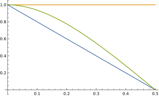
Figure 1. Comparison between the Fourier multipliers for the classical Hilbert transform (orange), the discrete Hilbert transform (blue), and the probabilistic discrete Hilbert transform (green).

Remark 7.5.

One can show that $\|\widetilde{M}\|_{\infty}=1$. This implies that $T_{\mathbb{H}}$ is bounded in $\ell^{2}(\mathbb{Z})$ and its norm is 1, as we already know. Since $\widetilde{M}$ is symmetric, periodic, $\widetilde{M}(0)=1$, and $\widetilde{M}(1/2)=0$, it suffices to show that $\widetilde{M}(\xi)$ is decreasing in $[0,\tfrac{1}{2}]$. Let $\varphi(x):=\psi(1+x)+\psi(1-x)-2\psi(1)$ where $\psi$ is the digamma function. Then, $\widetilde{M}$ can be written as

$$\widetilde{M}(\xi)=1+(1-2|\xi|)\varphi(|\xi|)+|\xi|(1-|\xi|)\varphi^{\prime}(|\xi|).$$

By the definition of $\psi$, $\varphi(x)$ has the integral representation

$$\varphi(x)=2\int_{0}^{\infty}\frac{1-\cosh(xy)}{e^{y}-1}\,dy.$$

It follows from this that $\frac{d^{n}}{dx^{n}}\varphi(x)\leq 0$ for all $n=0,1,2,\cdots$ and $x\in[0,\tfrac{1}{2}]$. Then,

$$\varphi(x) =-2x^{2}\sum_{n=1}^{\infty}\frac{1}{n(n^{2}-x^{2})},\qquad\varphi^{\prime}(x)=-4x\sum_{n=1}^{\infty}\frac{n}{(n^{2}-x^{2})^{2}}$$

$$\varphi^{\prime\prime}(x) =-4\sum_{n=1}^{\infty}\frac{n(n^{2}+3x^{2})}{(n^{2}-x^{2})^{3}}.$$

Thus,

$$\widetilde{M}^{\prime}(x) =-2\varphi(x)+2(1-2x)\varphi^{\prime}(x)+x(1-x)\varphi^{\prime\prime}(x)$$

$$=-4\sum_{n=1}^{\infty}\frac{1}{n(n^{2}-x^{2})^{3}}\left(-x^{2}(n^{2}-x^{2})^{2}+2(1-2x)n^{2}(n^{2}-x^{2})+x(1-x)n^{2}(n^{2}+3x^{2})\right).$$

The numerator in the summand can be written as

$$-x^{2}(n^{2}-x^{2})^{2}+2(1-2x)n^{2}(n^{2}-x^{2})+x(1-x)n^{2}(n^{2}+3x^{2})$$

$$\qquad=(1-2x)(2+x)n^{4}-x^{2}(x^{2}-7x+2)n^{2}-x^{6}$$

$$\qquad=(1-2x)(2+x)(n^{4}-n^{2})+((1-2x)(2+x)-x^{2}(x^{2}-7x+2)-x^{6})n^{2}+x^{6}(n^{2}-1)$$

$$\qquad=(1-2x)(2+x)(n^{4}-n^{2})-(x-1)^{2}(x^{4}+2x^{3}+4x^{2}-x-2)n^{2}+x^{6}(n^{2}-1).$$

Since $x^{4}+2x^{3}+4x^{2}-x-2\leq 0$ for all $x\in[0,\tfrac{1}{2}]$, we conclude that $\widetilde{M}^{\prime}(x)\leq 0$ for $x\in[0,\tfrac{1}{2}]$.

Recall that a function $u:\mathbb{R}^{d}\to\mathbb{C}$ is said to be positive-definite if for any $k\in\mathbb{N}$, $\xi_{1},\cdots,\xi_{k}\in\mathbb{R}^{d}$, $c_{1},\cdots,c_{k}\in\mathbb{C}$, it satisfies $\sum_{i,j=1}^{k}u(\xi_{i}-\xi_{j})c_{i}\overline{c_{j}}\geq 0$. A function $u:\mathbb{R}^{d}\to\mathbb{C}$ is called negative-definite if for any $k\in\mathbb{N}$, $\xi_{1},\cdots,\xi_{k}\in\mathbb{R}^{d}$, $c_{1},\cdots,c_{k}\in\mathbb{C}$,

$$\sum_{i,j=1}^{k}(u(\xi_{i})+\overline{u(\xi_{j})}-u(\xi_{i}-\xi_{j}))c_{i}\overline{c_{j}}\geq 0.$$

Bochner’s theorem (see [Jacob1]*Theorem 3.5.7, p.108) says that a function $u:\mathbb{R}^{d}\to\mathbb{C}$ is the Fourier transform of a probability measure $\mu$ if and only if $u$ is continuous and positive-definite with $u(0)=1$. Note that the definitions of positive-definite and negative-definite functions and Bochner’s theorem can be extended to functions on locally compact abelian groups in a natural way. In particular, if $u:Q\to\mathbb{C}$ is positive-definite and continuous with $u(0)=1$ where $Q=[-\tfrac{1}{2},\tfrac{1}{2})$, then there exists $(\mathcal{P}(n))_{n\in\mathbb{Z}}$ such that $\mathcal{P}(n)\geq 0$ for all $n\in\mathbb{Z}$, $\sum_{n\in\mathbb{Z}}\mathcal{P}(n)=1$, and $\mathcal{F}(\mathcal{P})(\xi)=u(\xi)$. See [BP68] for further information.

Lemma 7.6.

Suppose that a nonnegative continuous function $u:\mathbb{R}\to\mathbb{R}$ satisfies $u(\xi+n)=u(\xi)$ for all $\xi\in\mathbb{R}$, $n\in\mathbb{Z}$ and $u(0)=0$, and is increasing and concave on $[0,\tfrac{1}{2}]$. Then, there exists a probability kernel $(\mathcal{P}(n))_{n\in\mathbb{Z}}$ (that is, $\mathcal{P}(n)\geq 0$ and $\sum_{n\in\mathbb{Z}}\mathcal{P}(n)=1$) such that

$$\mathcal{F}(\mathcal{P})(\xi):=\sum_{n\in\mathbb{Z}}\mathcal{P}(n)e^{-2\pi in\xi}=\frac{1}{1+u(\xi)}.$$

Proof.

By Bochner’s theorem, it is enough to show that $(1+u(\xi))^{-1}$ is positive-definite. Let $v(\xi):=u(1/2)-u(\xi)$, then $v$ is decreasing and convex. By [Jacob1]*Theorem 3.5.22, we know that $v(\xi)\cdot\mathds{1}_{Q}(\xi)$ is positive-definite and so there exists a bounded nonnegative measure $\mu$ such that $\widehat{\mu}=v\cdot\mathds{1}_{Q}$ by Bochner’s theorem. Since a translation of a Fourier transform corresponds to a multiplication of a positive-definite function, $v(\xi)\cdot\mathds{1}_{3Q}(\xi)$ is also positive-definite. We claim that $v$ is positive-definite. Let $k\in\mathbb{N}$, $c_{1},\cdots,c_{k}\in\mathbb{C}$, and $\xi_{i}\in\mathbb{R}$. Since $v$ is periodic in $Q$, it suffices to consider $\xi_{i}\in Q$. Since $\xi_{i}-\xi_{j}\in 3Q$, we obtain

$$\sum_{i,j=1}^{k}v(\xi_{i}-\xi_{j})c_{i}\overline{c_{j}}=\sum_{i,j=1}^{k}v(\xi_{i}-\xi_{j})\mathds{1}_{3Q}(\xi_{i}-\xi_{j})c_{i}\overline{c_{j}}\geq 0$$

as desired. It then follows from [Jacob1]*Corollary 3.6.10 that $v(0)-v(\xi)=u(\xi)$ is negative-definite. By [Jacob1]*Corollary 3.6.13, we see that $(1+u(\xi))^{-1}$ is positive-definite. ∎

Proof of Theorem 7.1.

The Fourier multiplier for the classical discrete Hilbert transform $H_{\mathrm{dis}}$ with kernel $K_{{H}_{\mathrm{dis}}}(n)=\frac{1}{\pi n}$ is

$$\mathcal{F}(K_{{H}_{\mathrm{dis}}})(\xi)=\sum_{n\in\mathbb{Z}\setminus\{0\}}\frac{1}{\pi n}e^{-2\pi in\xi}=-\sum_{n\in\mathbb{Z}\setminus\{0\}}\frac{2i}{\pi n}\sin(2\pi n\xi)=-i\frac{\xi}{|\xi|}(1-2|\xi|)$$

for $\xi\in[-\frac{1}{2},-\frac{1}{2})$. Thus, we have

$$\mathcal{F}(K_{{H}_{\mathrm{dis}}})(\xi)=-i\frac{\xi}{|\xi|}(1-2|\xi|)=\mathcal{F}(K_{\mathbb{H}})(\xi)\frac{1-2|\xi|}{\widetilde{M}(\xi)}.$$

By this and Lemma 7.6, it is enough to show that $u(x):=\widetilde{M}(x)/(1-2|x|)-1$ is increasing and concave on $[0,1/2]$ with $u(0)=0$. Since $\widetilde{M}(0)=1$, we immediately have $u(0)=0$. Since

$$u(x) =\frac{1}{1-2x}+\varphi(x)+\frac{x(1-x)}{1-2x}\varphi^{\prime}(x)-1$$

$$=\frac{1}{4(1-2x)}(4+\varphi^{\prime}(x))+\varphi(x)-\frac{1-2x}{4}\varphi^{\prime}(x)-1,$$

$$u^{\prime}(x) =\frac{1}{2(1-2x)^{2}}(4+\varphi^{\prime}(x))+\frac{\varphi^{\prime\prime}(x)}{4(1-2x)}+\frac{3}{2}\varphi^{\prime}(x)-\frac{1-2x}{4}\varphi^{\prime\prime}(x),$$

it follows from L’hospital’s rule and the recurrence property of polygamma functions that

$$u^{\prime}(1/2)=-\frac{1}{16}\varphi^{\prime\prime\prime}(1/2)+\frac{3}{2}\varphi^{\prime}(1/2)=0.$$

Thus, it suffices to prove that $u^{\prime\prime}(x)\leq 0$ for $x\in[0,\tfrac{1}{2}]$. Let

$$v(x) :=(1-2x)^{3}u^{\prime\prime}(x)$$

$$=2(4+\varphi^{\prime}(x))+(1-2x)(1+2(1-2x)^{2})\varphi^{\prime\prime}(x)+x(1-x)(1-2x)^{2}\varphi^{\prime\prime\prime}(x).$$

Note that

$$v^{\prime}(x)=(1-2x)^{2}(-12\varphi^{(2)}(x)+4(1-2x)\varphi^{(3)}(x)+x(1-x)\varphi^{(4)}(x)).$$

Using the series representation for $\varphi(x)$ (see the remark above), we get

$$-12\varphi^{(2)}(x)+4(1-2x)\varphi^{(3)}(x)+x(1-x)\varphi^{(4)}(x)$$

$$\qquad=\sum_{n=1}^{\infty}\frac{n}{(n^{2}-x^{2})^{5}}(n^{6}-5x(1-2x)n^{4}-5x^{3}(2-x)n^{2}-x^{5})$$

$$\qquad=\sum_{n=1}^{\infty}\frac{n}{(n^{2}-x^{2})^{5}}((n^{6}-n^{4})+(1-x)^{5}n^{4}+5x^{3}(2-x)(n^{4}-n^{2})+(n^{4}-1)x^{5})\geq 0$$

for all $x\in[0,\tfrac{1}{2}]$. Since $v^{\prime}(x)\geq 0$ and $v(1/2)=0$, we obtain that $v(x)\leq 0$ and so $u^{\prime\prime}(x)\leq 0$ for $x\in[0,\tfrac{1}{2}]$ as desired. By Lemma 7.6, we conclude that there exists a probability kernel $\mathcal{P}$ such that $H_{\mathrm{dis}}=T_{\mathbb{H}}\ast\mathcal{P}$. ∎

Question 7.7.

Does Theorem 7.1 hold for $d>1$? More precisely, is there a probability kernel $\mathcal{P}^{(k)}$ on $\mathbb{Z}^{d}$ such that

$$R_{\mathrm{dis}}^{(k)}f(n)=\sum_{m\in\mathbb{Z}^{d}}\mathcal{P}^{(k)}(n-m)T_{\mathbb{H}^{(k)}}f(m)?$$

8. Probabilistic continuous Riesz transforms

Given that discrete operators obtained from Calderón–Zygmund kernels as defined in (5.3) simply by replacing the continuous variable $z$ by the discrete variable $n$ and avoiding the singularity at $\{0\}$ in the sum are bounded on $\ell^{p}$ (Propostion 5.1), it is natural to ask if the the opposite is also true in the current situation. More precisely, is it true that the kernels obtained from $K_{\mathbb{H}^{(k)}}$ simply by replacing $k\in\mathbb{Z}^{d}$ with $z\in\mathbb{R}^{d}$, $|z|\geq 1$, together with the some modification for $|z|<1$, are Calderón–Zygmund kernels satisfying (5.3)? In this section we give a formula for such continuous kernels that satisfy (5.3), with the exception of the $C^{1}$ property on the sphere $|z|=1$, and are also bounded on $L^{p}(\mathbb{R}^{d})$, $1<p<\infty$ with rather precise norm bounds. Since we are able to find various explicit constants for the case $d=1$, we consider the cases $d=1$ and $d>1$ separately.

From formula (6.8) a natural version of a continuous kernel which gives the probabilistic discrete Hilbert transform à la Calderón–Zygmund would be

(8.1) $$\mathbb{K}_{\mathbb{H}}(z)=\frac{1}{\pi z}\left(1+\int_{0}^{\infty}\frac{2y^{3}}{(y^{2}+\pi^{2}z^{2})\sinh^{2}(y)}\,dy\right)\,\mathds{1}_{\{|z|\geq 1\}}(z)+\frac{1}{\pi z}\mathds{1}_{\{|z|<1\}}(z),\quad z\in\mathbb{R}.$$

Similarly, for $d>1$ from (6.7) a natural definition of version of a continuous kernel which gives the probabilistic discrete Riesz transforms for $k=1,2,\dots,d$ would be

(8.2) $$\mathbb{K}_{\mathbb{H}^{(k)}}(z): =\left(-4\int_{\mathbb{R}^{d}}\int_{0}^{\infty}\frac{1}{h(x,y)}\frac{\partial{p_{0}}}{\partial x_{k}}\frac{\partial}{\partial y}(yp_{z})\,dydx\right)\mathds{1}_{\{|z|\geq 1\}}(z)+c_{d}\frac{z_{k}}{|z|^{d+1}}\mathds{1}_{\{|z|<1\}}(z)$$

$$=\left(I_{1}(z)+I_{2}(z)\right)\mathds{1}_{\{|z|\geq 1\}}(z)+c_{d}\frac{z_{k}}{|z|^{d+1}}\mathds{1}_{\{|z|<1\}}(z),$$

where

$$I_{1}^{(k)}(z)=\int_{\mathbb{R}^{d}}\int_{0}^{\infty}\frac{8c_{d}^{2}(d+1)x_{k}y^{2}}{h(x,y)(|x|^{2}+y^{2})^{\frac{d+3}{2}}(|x-z|^{2}+y^{2})^{\frac{d+1}{2}}}\,dxdy,$$

and

$$I_{2}^{(k)}(z)=-\int_{\mathbb{R}^{d}}\int_{0}^{\infty}\frac{4c_{d}^{2}(d+1)^{2}x_{k}y^{4}}{h(x,y)(|x|^{2}+y^{2})^{\frac{d+3}{2}}(|x-z|^{2}+y^{2})^{\frac{d+3}{2}}}\,dxdy$$

and $c_{d}=\Gamma(\frac{d+1}{2})\pi^{-\frac{d+1}{2}}$.

Notice that $\mathbb{K}_{\mathbb{H}^{(k)}}$ is not continuous on $|z|=1$ and hence not a Calderón–Zygmund kernel requiring (5.3). Nevertheless, with these definition we have

Theorem 8.1.

For any $d\geq 1$ and $k=1,\dots d$, the kernels $\mathbb{K}_{\mathbb{H}^{(k)}}(z)$ ($\mathbb{K}_{\mathbb{H}}(z)$ when $d=1$) satisfy

• (8.3) $$|\mathbb{K}_{\mathbb{H}^{(k)}}(z)|\leq\frac{C_{d}}{|z|^{d}},\quad z\in\mathbb{R}^{d}\setminus\{0\}.$$

• (8.4) $$|\nabla\mathbb{K}_{\mathbb{H}^{(k)}}(z)|\leq\frac{C_{d}}{|z|^{d+1}},\quad z\in\mathbb{R}^{d}\setminus\{0\},\quad|z|\neq 1,$$

  where $C_{d}$ depends only on $d$. Furthermore,

• For $d=1$,

  (8.5) $$\sup_{\xi\in\mathbb{R}}|\widehat{\mathbb{K}_{\mathbb{H}}}(\xi)|\leq 1+\frac{2}{\pi}\int_{0}^{\infty}\frac{y\ln(y^{2}/\pi^{2}+1)}{\sinh^{2}(y)}dy\approx 1.09956.$$

• For $d>1$ and all $k=1,\dots d$, we have

  (8.6) $$|\widehat{\mathbb{K}_{\mathbb{H}^{(k)}}}(\xi)|\leq C_{d},\quad\text{for all}\quad\xi\in\mathbb{R}^{d}\setminus\{0\}$$

Proof.

We first show the case $d=1$ which is computationally much simper and will give explicit constants, particularly the bound for the Fourier transform. Clearly $|\mathbb{K}_{\mathbb{H}}(z)|=\frac{1}{\pi|z|}$, for $0<|z|<1$. On the other hand, since

$$\int_{0}^{\infty}\frac{y^{3}}{(y^{2}+\pi^{2}z^{2})\sinh^{2}(y)}\,dy \leq\frac{1}{\pi^{2}z^{2}}\int_{0}^{\infty}\frac{y^{3}}{\sinh^{2}(y)}\,dy$$

$$=\frac{4}{\pi^{2}z^{2}}\int_{0}^{\infty}\frac{y^{3}}{e^{2y}(1-e^{-2y})^{2}}\,dy$$

$$=\frac{4}{\pi^{2}z^{2}}\sum_{k=1}^{\infty}k\int_{0}^{\infty}y^{3}e^{-2ky}\,dy$$

(8.7) $$=\frac{3}{2\pi^{2}z^{2}}\sum_{k=1}^{\infty}\frac{1}{k^{3}}=\frac{3}{2\pi^{2}z^{2}}\zeta(3).$$

From this it follows that $|\mathbb{K}(z)|\leq\frac{C_{1}}{|z|}$, for all $|z|>0$. Similarly, for $|z|\geq 1$,

$$|K_{\mathbb{H}}^{\prime}(z)| =\left|-\frac{1}{\pi z^{2}}\left(1+\int_{0}^{\infty}\frac{2y^{3}}{(y^{2}+\pi^{2}z^{2})\sinh^{2}(y)}\,dy\right)-\int_{0}^{\infty}\frac{4y^{3}}{(y^{2}+\pi^{2}z^{2})^{2}\sinh^{2}(y)}\,dy\right|$$

$$\leq\frac{C_{2}}{|z|^{2}},$$

and again we have $|K_{\mathbb{H}}^{\prime}(z)|\leq\frac{C}{|z|^{2}}$ for all $|z|>0$, $|z|\neq 1$. Here, $\kappa$ is a universal constant. Thus $\mathbb{K}_{\mathbb{H}}$ satisfies (i) and (ii).

In addition, we have, in the principal value sense,

$$\widehat{\mathbb{K}}(\xi) =\int_{\mathbb{R}}\mathbb{K}(z)e^{-2\pi iz\cdot\xi}dz$$

(8.8) $$=\int_{\mathbb{R}}\frac{1}{\pi z}e^{-2\pi iz\cdot\xi}dz+\frac{1}{\pi}\int_{0}^{\infty}\frac{2y^{3}}{\sinh^{2}(y)}\,\left(\int_{\{|z|>1\}}\frac{e^{-2\pi iz\cdot\xi}}{z(y^{2}+\pi^{2}z^{2})}\,dz\right)\,dy$$

$$=-i\operatorname{sign}(\xi)+\frac{1}{\pi}\int_{0}^{\infty}\frac{2y^{3}}{\sinh^{2}(y)}\,\left(\int_{\{|z|>1\}}\frac{e^{-2\pi iz\cdot\xi}}{z(y^{2}+\pi^{2}z^{2})}\,dz\right)\,dy$$

$$=-i\operatorname{sign}(\xi)\left(1+\frac{1}{\pi}\int_{0}^{\infty}\frac{2y^{3}}{\sinh^{2}(y)}\,\left(\int_{\{|z|>1\}}\frac{\sin(2\pi z|\xi|)}{z(y^{2}+\pi^{2}z^{2})}\,dz\right)\,dy\right).$$

By Fubini and the identity, obtained by integration by parts,

$$\int_{1}^{\infty}\frac{1}{z(y^{2}+\pi^{2}z^{2})}dz=\frac{\ln(y^{2}/\pi^{2}+1)}{2y^{2}},$$

we have

$$\Big{|}\frac{1}{\pi}\int_{0}^{\infty}\frac{y^{3}}{\sinh^{2}(y)}\,\left(\int_{\{|z|>1\}}\frac{e^{-2\pi iz\cdot\xi}}{z(y^{2}+\pi^{2}z^{2})}\,dz\right)\,dy\Big{|} \leq\frac{2}{\pi}\int_{0}^{\infty}\frac{y^{3}}{\sinh^{2}(y)}\,\left(\int_{1}^{\infty}\frac{1}{z(y^{2}+\pi^{2}z^{2})}\,dz\right)\,dy$$

$$=\frac{1}{\pi}\int_{0}^{\infty}\frac{y\ln(y^{2}/\pi^{2}+1)}{\sinh^{2}(y)}dy$$

(8.9) $$\approx 0.0497822.$$

Hence for all $\xi\in\mathbb{R}$,

$$|\widehat{\mathbb{K}}(\xi)|\leq 1+\frac{2}{\pi}\int_{0}^{\infty}\frac{y\ln(y^{2}/\pi^{2}+1)}{\sinh^{2}(y)}dy\approx 1.09956,$$

which is the claim in (iii).

We now suppose $d>1$. By (6.11) and a change of variables we have, for $|z|\geq 1$ and $z=|z|\theta$, that

$$|K_{\mathbb{H}^{(k)}}(z)| \leq C_{d}\int_{0}^{\infty}\int_{\mathbb{R}^{d}}\frac{y}{(|x|^{2}+y^{2})^{\frac{d+1}{2}}(|x-z|^{2}+y^{2})^{\frac{d+1}{2}}}\,dxdy$$

$$=\frac{C_{d}}{|z|^{d}}\int_{0}^{\infty}\int_{\mathbb{R}^{d}}\frac{y}{(|x|^{2}+y^{2})^{\frac{d+1}{2}}(|x-\theta|^{2}+y^{2})^{\frac{d+1}{2}}}\,dxdy.$$

Since

$$\int_{0}^{\infty}\int_{\mathbb{R}^{d}}\frac{y}{(|x|^{2}+y^{2})^{\frac{d+1}{2}}(|x-\theta|^{2}+y^{2})^{\frac{d+1}{2}}}\,dxdy \leq\int_{0}^{\infty}\int_{\{|x-\theta|\leq\frac{1}{2}\}}\frac{y}{(\frac{1}{4}+y^{2})^{\frac{d+1}{2}}(|x-\theta|^{2}+y^{2})^{\frac{d+1}{2}}}\,dxdy$$

$$\qquad+\int_{0}^{\infty}\int_{\{|x-\theta|\geq\frac{1}{2}\}}\frac{y}{(|x|^{2}+y^{2})^{\frac{d+1}{2}}(\frac{1}{4}+y^{2})^{\frac{d+1}{2}}}\,dxdy$$

$$\leq\int_{0}^{\infty}\frac{C_{d}}{(1+y^{2})^{\frac{d+1}{2}}}\int_{\mathbb{R}^{d}}\frac{1}{(|x|^{2}+1)^{\frac{d+1}{2}}}\,dxdy\leq C_{d}.$$

This together with the obvious bound for the second term in (8.2) gives that $|K_{\mathbb{H}^{(k)}}(z)|\leq\frac{C_{d}}{|z|^{d}}$, for $|z|>0$. Next, for $j=1,2,\cdots,d$, differentiation and (3.4) gives that for $|z|>1$,

$$\Big{|}\frac{\partial}{\partial z_{j}}I_{1}^{(k)}(z)\Big{|} =C_{d}\Big{|}\int_{0}^{\infty}\int_{\mathbb{R}^{d}}\frac{x_{k}y^{2}(x_{j}-z_{j})}{h(x,y)(|x|^{2}+y^{2})^{\frac{d+3}{2}}(|x-z|^{2}+y^{2})^{\frac{d+3}{2}}}\,dxdy\Big{|}$$

$$\leq\frac{C_{d}}{|z|^{(d+1)}}\int_{0}^{\infty}\int_{\mathbb{R}^{d}}\frac{|x_{k}x_{j}|y}{(|x|^{2}+y^{2})^{\frac{d+2}{2}}(|x-\theta|^{2}+y^{2})^{\frac{d+3}{2}}}\,dxdy$$

$$\qquad+\frac{C_{d}|z_{j}|}{|z|^{(d+2)}}\int_{0}^{\infty}\int_{\mathbb{R}^{d}}\frac{|x_{k}z_{j}|y}{(|x|^{2}+y^{2})^{\frac{d+2}{2}}(|x-\theta|^{2}+y^{2})^{\frac{d+3}{2}}}\,dxdy$$

$$\leq\frac{C_{d}}{|z|^{d+1}},$$

where $z=|z|\theta$. Similarly, we can obtain the same upper bound for $\frac{\partial}{\partial z_{j}}I_{2}^{(k)}(z)$, $|z|>1$, which leads to $\big{|}\nabla{\mathbb{K}_{\mathbb{H}^{(k)}}(z)}\big{|}\leq\frac{C_{d}}{|z|^{d+1}}$ for all $|z|>0$ and $|z|\neq 1$.

It remains to show that the Fourier transform of $\mathbb{K}^{(k)}(z)$ is bounded. By (6.7) and Proposition 6.5, we have that

(8.10) $$-4\int_{\mathbb{R}^{d}}\int_{0}^{\infty}\frac{\partial p_{0}(x,y)}{\partial x_{k}}\frac{\partial}{\partial y}(yp_{z}(x,y))\,dydx=\frac{c_{d}z_{k}}{|z|^{d+1}},\quad|z|>0.$$

This formula can also be easily verified using the Fourier transform. More precisely, we have

$$-4\int_{\mathbb{R}^{d}}\int_{\mathbb{R}^{d}}\int_{0}^{\infty}\frac{\partial p}{\partial x_{k}}(x,y)\frac{\partial}{\partial y}(yp(x-z,y))e^{-2\pi iz\cdot\xi}\,dydxdz$$

$$=-4\int_{\mathbb{R}^{d}}\int_{0}^{\infty}\frac{\partial p}{\partial x_{k}}(x,y)\frac{\partial}{\partial y}(ye^{-2\pi|\xi|y})e^{-2\pi ix\cdot\xi}\,dydx$$

$$=-8\pi i\xi_{k}\int_{0}^{\infty}(1-2\pi|\xi|y)e^{-4\pi|\xi|y}\,dy$$

$$=-i\frac{\xi_{k}}{|\xi|},$$

which implies (8.10). Thus we can write (8.2) as

(8.11) $$\mathbb{K}_{\mathbb{H}^{(k)}}(z)=\left(-4\int_{0}^{\infty}\int_{\mathbb{R}^{d}}\left(\frac{1}{h}-1\right)\frac{\partial p_{0}(x,y)}{\partial x_{k}}\frac{\partial}{\partial y}(yp_{z}(x,y))\,dxdy\right)\mathds{1}_{\{|z|\geq 1\}}(z)+c_{d}\frac{\,z_{k}}{|z|^{d+1}}.$$

Since the Fourier transform of the second term is $-i\frac{\xi_{k}}{|\xi|}$ (the Fourier transform of the classical Riesz transforms), it is enough to show that

$$\int_{\{|z|\geq 1\}}J_{1}^{(k)}(z)e^{-2\pi iz\cdot\xi}\,dz,\quad\int_{\{|z|\geq 1\}}J_{2}^{(k)}(z)e^{-2\pi iz\cdot\xi}\,dz$$

are uniformly bounded in $\xi$, where

(8.12) $$J_{1}^{(k)}(z) :=\int_{0}^{\infty}\int_{\mathbb{R}^{d}}\left(\frac{1}{h(x,y)}-1\right)\frac{x_{k}y^{2}}{(|x|^{2}+y^{2})^{\frac{d+3}{2}}(|x-z|^{2}+y^{2})^{\frac{d+1}{2}}}\,dxdy,$$

(8.13) $$J_{2}^{(k)}(z) :=\int_{0}^{\infty}\int_{\mathbb{R}^{d}}\left(\frac{1}{h(x,y)}-1\right)\frac{x_{k}y^{4}}{(|x|^{2}+y^{2})^{\frac{d+3}{2}}(|x-z|^{2}+y^{2})^{\frac{d+3}{2}}}\,dxdy.$$

By the estimate (3.4), $|\frac{1}{h(x,y)}-1|\leq C_{d}\frac{\sqrt{x^{2}+y^{2}}}{y}$, and

(8.14) $$\int_{\{|x|\geq\frac{1}{2}\}}(|x|^{2}+y^{2})^{-\frac{d+1}{2}}\,dx\leq\int_{\{|x|\geq\frac{1}{2}\}}|x|^{-(d+1)}\,dx\leq C_{d}$$

for $0\leq y\leq 1$ we have

$$\int_{\{|z|\geq 1\}}\int_{0}^{1}\int_{\{|x|\leq\frac{1}{2}\}}\left|\frac{1}{h(x,y)}-1\right|\frac{|x_{k}|y^{2}}{(|x|^{2}+y^{2})^{\frac{d+3}{2}}(|x-z|^{2}+y^{2})^{\frac{d+1}{2}}}\,dxdydz$$

$$\leq\int_{0}^{1}\int_{\{|x|\leq\frac{1}{2}\}}\left(\int_{\{|x-z|\geq\frac{1}{2}\}}\frac{1}{(|x-z|^{2}+y^{2})^{\frac{d+1}{2}}}\,dz\right)\left|\frac{1}{h(x,y)}-1\right|\frac{|x_{k}|y^{2}}{(|x|^{2}+y^{2})^{\frac{d+3}{2}}}\,dxdy$$

$$\leq C_{d}\int_{0}^{1}\int_{\{|x|\leq\frac{1}{2}\}}\frac{y}{(|x|^{2}+y^{2})^{\frac{d+1}{2}}}\,dxdy\leq C_{d}.$$

Note that in the first inequality, we used the fact that if $|x|\leq\frac{1}{2}$ and $|z|\geq 1$, then $|x-z|\geq\frac{1}{2}$. Similarly,

$$\int_{\{|z|\geq 1\}}\int_{1}^{\infty}\int_{\{|x|\leq\frac{1}{2}\}}\left|\frac{1}{h(x,y)}-1\right|\frac{|x_{k}|y^{2}}{(|x|^{2}+y^{2})^{\frac{d+3}{2}}(|x-z|^{2}+y^{2})^{\frac{d+1}{2}}}\,dxdydz$$

$$\leq C_{d}\int_{1}^{\infty}\left(\int_{\{|x|\geq\frac{1}{2}\}}\frac{1}{(|x|^{2}+y^{2})^{\frac{d+1}{2}}}\,dx\right)\left(\int_{\{|x|\leq\frac{1}{2}\}}\left|\frac{1}{h(x,y)}-1\right|\frac{|x_{k}|y^{2}}{(|x|^{2}+y^{2})^{\frac{d+3}{2}}}\,dx\right)\,dy$$

$$\leq C_{d}\int_{1}^{\infty}\int_{\{|x|\leq\frac{1}{2}\}}y^{-d-1}\,dxdy\leq C_{d}.$$

On the other hand, it follows from (3.4), (8.14), and the bound

(8.15) $$\int_{\{|z|\geq 1\}}\frac{y}{(|x-z|^{2}+y^{2})^{\frac{d+1}{2}}}\,dz\leq C_{d}$$

that

$$\int_{\{|z|\geq 1\}}\int_{0}^{1}\int_{\{|x|\geq\frac{1}{2}\}}\left|\frac{1}{h(x,y)}-1\right|\frac{|x_{k}|y^{2}}{(|x|^{2}+y^{2})^{\frac{d+3}{2}}(|x-z|^{2}+y^{2})^{\frac{d+1}{2}}}\,dxdydz$$

$$=\int_{0}^{1}\int_{\{|x|\geq\frac{1}{2}\}}\left(\int_{\{|z|\geq 1\}}\frac{y}{(|x-z|^{2}+y^{2})^{\frac{d+1}{2}}}\,dz\right)\left|\frac{1}{h(x,y)}-1\right|\frac{|x_{k}|y}{(|x|^{2}+y^{2})^{\frac{d+3}{2}}}\,dxdy$$

$$\leq C_{d}\int_{0}^{1}\int_{\{|x|\geq\frac{1}{2}\}}\left|\frac{1}{h(x,y)}-1\right|\frac{|x_{k}|y}{(|x|^{2}+y^{2})^{\frac{d+3}{2}}}\,dxdy$$

$$\leq C_{d}\int_{0}^{1}\int_{\{|x|\geq\frac{1}{2}\}}\frac{1}{(|x|^{2}+y^{2})^{\frac{d+1}{2}}}\,dxdy\leq C_{d}.$$

By Lemma 3.1, we know that $|1/h(x,y)-1|\leq\frac{C_{d}}{y}$ for $y\geq 1$. Using this,

$$\int_{\{|z|\geq 1\}}\int_{1}^{\infty}\int_{\{|x|\geq\frac{1}{2}\}}\left|\frac{1}{h(x,y)}-1\right|\frac{|x_{k}|y^{2}}{(|x|^{2}+y^{2})^{\frac{d+3}{2}}(|x-z|^{2}+y^{2})^{\frac{d+1}{2}}}\,dxdydz$$

$$=\int_{1}^{\infty}\int_{\{|x|\geq\frac{1}{2}\}}\left(\int_{\{|z|\geq 1\}}\frac{y}{(|x-z|^{2}+y^{2})^{\frac{d+1}{2}}}\,dz\right)\left|\frac{1}{h(x,y)}-1\right|\frac{|x_{k}|y}{(|x|^{2}+y^{2})^{\frac{d+3}{2}}}\,dxdy$$

$$\leq C_{d}\int_{1}^{\infty}\int_{\{|x|\geq\frac{1}{2}\}}\frac{1}{(|x|^{2}+y^{2})^{\frac{d+2}{2}}}\,dxdy$$

$$\leq C_{d}\int_{1}^{\infty}\frac{1}{y^{2}}\,dy\int_{\mathbb{R}^{d}}\frac{1}{(|w|^{2}+1)^{\frac{d+2}{2}}}\,dw\leq C_{d}.$$

In the last inequality, we have used the change of variable $wy=x$. Thus, we get

(8.16) $$\left|\int_{\{|z|\geq 1\}}J_{1}^{(k)}(z)e^{-2\pi iz\cdot\xi}\,dz\right|\leq\int_{\{|z|\geq 1\}}|J_{1}^{(k)}(z)|\,dz\leq C_{d}.$$

Using the trivial bound $y^{2}/(|x-z|^{2}+y^{2})\leq 1$, it follows from the previous argument that

$$\left|\int_{\{|z|\geq 1\}}J_{2}^{(k)}(z)e^{-2\pi iz\cdot\xi}\,dz\right|$$

$$\leq\int_{\{|z|\geq 1\}}\int_{0}^{\infty}\int_{\mathbb{R}^{d}}\left|\frac{1}{h(x,y)}-1\right|\frac{|x_{k}|y^{4}}{(|x|^{2}+y^{2})^{\frac{d+3}{2}}(|x-z|^{2}+y^{2})^{\frac{d+3}{2}}}\,dxdydz$$

$$\leq\int_{\{|z|\geq 1\}}\int_{0}^{\infty}\int_{\mathbb{R}^{d}}\left|\frac{1}{h(x,y)}-1\right|\frac{|x_{k}|y^{2}}{(|x|^{2}+y^{2})^{\frac{d+3}{2}}(|x-z|^{2}+y^{2})^{\frac{d+1}{2}}}\,dxdydz$$

$$\leq C_{d}.$$

∎

Remark 8.2.

Note that the proof of the boundedness of the Fourier transform for $d=1$ shows that in fact the function

$$J(z)=\frac{1}{\pi z}\left(\int_{0}^{\infty}\frac{2y^{3}}{(y^{2}+\pi^{2}z^{2})\sinh^{2}(y)}\,dy\right)\,\mathds{1}_{\{|z|\geq 1\}}(z)$$

is in $L^{1}(\mathbb{R})$ with $\|J\|_{L^{1}}\approx 0.09956$. Similarly, for $d>1$, the proof shows that $J_{1}^{(k)}(z)\mathds{1}_{\{|z|\geq 1\}}(z)$ and $J_{2}^{(k)}(z)\mathds{1}_{\{|z|\geq 1\}}(z)$ are in $L^{1}(\mathbb{R}^{d})$ with bounds depending only on $d$.

This gives the following

Corollary 8.3.

For $d=1$, the continuous probabilistic Hilbert transform is given by

$$\mathbb{K}_{\mathbb{H}}(z) =\frac{1}{\pi z}\left(1+\int_{0}^{\infty}\frac{2y^{3}}{(y^{2}+\pi^{2}z^{2})\sinh^{2}(y)}\,dy\right)\,\mathds{1}_{\{|z|\geq 1\}}(z)+\frac{1}{\pi z}\mathds{1}_{\{|z|<1\}}(z)$$

(8.17) $$=J(z)+\frac{1}{\pi z},$$

where $\|J\|_{L^{1}}\approx 0.09956$.

Similarly for $d>1$,

(8.18) $$\mathbb{K}_{\mathbb{H}^{(k)}}(z) =J_{1}^{(k)}+J_{2}^{(k)}+c_{d}\frac{\,z_{k}}{|z|^{d+1}},$$

$$=J^{(k)}+c_{d}\frac{\,z_{k}}{|z|^{d+1}},$$

where $\|J^{(k)}\|_{L^{1}}\leq C_{d}$ where $C_{d}$ depends only on $d$.

We record the $L^{p}$-boundedness of the operators in the following Corollary.

Corollary 8.4.

With $J$ and $J^{(k)}$ as above, the probabilistic continuous Hilbert and Riesz transforms are of the form:

(8.19) $$\mathbb{K}_{\mathbb{H}}*f =J*f+Hf,$$

(8.20) $$\mathbb{K}_{\mathbb{H}^{(k)}}*f =J^{(k)}*f+R^{(k)}*f,\quad k=1,\dots,d.$$

For $1<p<\infty$,

(8.21) $$\|\mathbb{K}_{\mathbb{H}}\|_{L^{p}\to L^{p}}\leq\|J\|_{L^{1}}+\cot(\pi/(2p^{\ast}))\approx 0.09956+\cot(\pi/(2p^{\ast}))$$

and

(8.22) $$\|\mathbb{K}_{\mathbb{H}^{(k)}}\|_{L^{p}\to L^{p}}\leq\|J^{(k)}\|_{L^{1}}+\cot(\pi/(2p^{\ast}))\leq C_{d}+\cot(\pi/(2p^{\ast})),$$

where $C_{d}$ depends on the dimension $d$.

We conjecture that the $L^{p}$-norm of the operator $\mathbb{K}_{\mathbb{H}^{(k)}}$ is independent of $d$. As to the sharp value, that is not easy to guess with the information at hand.

Our proof above shows that the choice for the second terms in (8.1) and (8.2) is quite natural given the relationship of the first term to the Hilbert and Riesz transforms. The question of choosing different second terms in (8.1) and (8.2) that could lead to continuous operators with smaller $p$ norms, perhaps even $\cot(\pi/(2p^{\ast}))$, would be interesting to explore.

Remark 8.5.

Recall that the smoothness condition $|\nabla K(z)|\leq\kappa|z|^{-(d+1)}$ can be relaxed with Hörmander’s condition

(8.23) $$\sup_{y\neq 0}\int_{|x|\geq 2|y|}|K(x-y)-K(x)|\,dx\leq B<\infty,$$

see [Graf]*Theorem 4.3.3 and [Stein70]*Corollary on p.34, Theroem 2, p.35. In particular, if $K$ satisfies $|K(x)|\leq\kappa|x|^{-d}$ and Hörmander’s condition, then the convolution operator $T$ with kernel $K$ is bounded on $L^{p}$, $1<p<\infty$. We claim that the kernel $\mathbb{K}_{\mathbb{H}^{(k)}}$ satisfies Hörmander’s condition. We have already seen that

$$|\nabla\mathbb{K}_{\mathbb{H}^{(k)}}(x)|\leq\frac{C}{|x|^{d+1}},\quad\text{for }|x|\neq 0,1.$$

Suppose $|y|>1$. If $|x|\geq 2|y|$ then

$$|\theta(x-y)+(1-\theta)x|=|x-\theta y|\geq(1-\tfrac{\theta}{2})|x|\geq(2-\theta)|y|$$

for all $0\leq\theta\leq 1$. By Taylor’s theorem, we have

$$|\mathbb{K}_{\mathbb{H}^{(k)}}(x-y)-\mathbb{K}_{\mathbb{H}^{(k)}}(x)|\leq|\nabla\mathbb{K}_{\mathbb{H}^{(k)}}(x-\theta y)||y|\leq\frac{C|y|}{|x-\theta y|^{d+1}}\leq\frac{C|y|}{|x|^{d+1}},$$

which leads to

$$\int_{|x|\geq 2|y|}|\mathbb{K}_{\mathbb{H}^{(k)}}(x-y)-\mathbb{K}_{\mathbb{H}^{(k)}}(x)|\,dx\leq C|y|\int_{2|y|}^{\infty}\frac{1}{r^{2}}\,dr\leq C<\infty.$$

If $|y|\leq 1$ and $|x|>|y|+1$, then $|x-\theta y|>1$ for $0\leq\theta\leq 1$. Thus, the same argument yields

$$\int_{|x|\geq|y|+1}|\mathbb{K}_{\mathbb{H}^{(k)}}(x-y)-\mathbb{K}_{\mathbb{H}^{(k)}}(x)|\,dx\leq C<\infty.$$

Let $\tfrac{1}{4}<|y|\leq 1$ and $2|y|\leq|x|\leq|y|+1$. Using $|\mathbb{K}_{\mathbb{H}^{(k)}}(x)|\leq\kappa|x|^{-d}$ and $|x-y|\geq\tfrac{1}{2}|x|$, we get

$$\int_{2|y|\leq|x|\leq|y|+1}|\mathbb{K}_{\mathbb{H}^{(k)}}(x-y)-\mathbb{K}_{\mathbb{H}^{(k)}}(x)|\,dx\leq C\int_{2|y|\leq|x|\leq|y|+1}|x|^{-d}\,dx=C\left|\log\left(\frac{|y|+1}{2|y|}\right)\right|,$$

which is bounded for $|y|\in(\tfrac{1}{4},1]$. Suppose $|y|\leq\tfrac{1}{4}$ and $\tfrac{3}{4}\leq|x|\leq|y|+1$, then the same argument gives

$$\int_{\tfrac{3}{4}\leq|x|\leq|y|+1}|\mathbb{K}_{\mathbb{H}^{(k)}}(x-y)-\mathbb{K}_{\mathbb{H}^{(k)}}(x)|\,dx\leq C\int_{\tfrac{3}{4}\leq|x|\leq|y|+1}|x|^{-d}\,dx=C|\log(\tfrac{4}{3}(|y|+1))|<\infty.$$

If $|y|\leq\tfrac{1}{4}$ and $2|y|\leq|x|<\tfrac{3}{4}$, then $|x-\theta y|<1$. Thus it follows from the gradient bound that

$$\int_{2|y|\leq|x|<\frac{3}{4}}|\mathbb{K}_{\mathbb{H}^{(k)}}(x-y)-\mathbb{K}_{\mathbb{H}^{(k)}}(x)|\,dx\leq C|y|\int_{2|y|}^{\frac{3}{4}}\frac{1}{r^{2}}\,dr\leq C<\infty.$$

Therefore the kernel $\mathbb{K}_{\mathbb{H}^{(k)}}$ satisfies Hörmander’s condition and the $L^{p}(\mathbb{R}^{d})$-boundedness of the operators for $1<p<\infty$ also follows from the Calderón–Zygmund theory.

9. A method of rotations for discrete Riesz trasforms

Given the fact that the classical method of rotations can be used to show that the Riesz transforms (and other singular integrals) in $\mathbb{R}^{d}$ have norms bounded above by the norm of the Hilbert transform, as discussed in Section 5.2, it is natural to ask if there is a discrete version of such a technique that would reduce the boundedness of operators on $\ell^{p}(\mathbb{Z}^{d})$ (with some assumptions on their kernel) to the boundedness of $H_{\mathrm{dis}}$ on $\ell^{p}(\mathbb{Z})$. While this does not seem to be the case for the setting of the CZ discrete Riesz transform as defined in (5.14), we can define closely related operators for which such a procedure is possible.

9.1. Two-dimensional case

We first consider the $d=2$ case where a particularly simple expression for the discrete transform is available. For $j=1,2$, from (5.6) we have

$$R^{(i)}f(x) =\frac{1}{2\pi}\,\mathrm{p.v.\!}\int_{\mathbb{R}^{2}}f(y)\,\frac{x_{i}-y_{i}}{|x-y|^{3}}\,dy.$$

Note that

$$\frac{\partial^{2}|y|}{\partial y_{j}^{2}}=\frac{1}{|y|}-\frac{y_{j}^{2}}{|y|^{3}}=\frac{|y|^{2}-y_{j}^{2}}{|y|^{3}}=\frac{y_{i}^{2}}{|y|^{3}}\,,$$

where $i=1$, if $j=2$ and $i=2$, if $j=1$. Hence, the kernel of $R^{(i)}$ is given by

$$\frac{1}{y_{i}}\frac{\partial^{2}|y|}{\partial y_{j}^{2}}\,.$$

Although not necessarily natural, this motivates the following definition for a different variant of discrete Riesz transforms

$$\mathcal{R}^{(i)}f(n)=\frac{1}{2\pi}\sum_{m\in\mathbb{Z}^{2}}f(m)\frac{|n-m+e_{j}|+|n-m-e_{j}|-2|n-m|}{{n_{i}-m_{i}}}\mathds{1}_{\{{m_{i}\neq n_{i}}\}}.$$

For simplicity, we consider ${i}=1$. Fix $a,b\in\mathbb{R}$ and define the directional discrete Hilbert transform via the formula

$$\mathcal{H}_{a,b}f(n) =\frac{1}{\pi}\sum_{m\in\mathbb{Z}^{2}}\frac{f(m)}{n_{1}-m_{1}}\,\mathds{1}_{\{n_{1}\neq m_{1},n_{2}-\lfloor an_{1}+b\rfloor=m_{2}-\lfloor am_{1}+b\rfloor\}}.$$

The intuition behind this definition is as follows. We split $\mathbb{Z}^{2}$ into an infinite family of “one-dimensional” sets

$$F_{a,b,l} =\{(k,\lfloor ak+b\rfloor+l):k\in\mathbb{Z}\}=\{n\in\mathbb{Z}^{2}:n_{2}-\lfloor an_{1}+b\rfloor=l\},$$

where $l$ takes arbitrary integer values. Then $\mathcal{H}_{a,b}$ acts as a (one-dimensional) discrete Hilbert transform on each of the fibers $F_{a,b,l}$. In particular, the above interpretation combined with Corollary 7.2 immediately gives that

$$\|\mathcal{H}_{a,b}\|_{p\to p} =\cot(\tfrac{\pi}{2p^{*}}),$$

which is the norm of the continuous Hilbert transform.

Theorem 9.1.

For compactly supported $f:\mathbb{Z}^{2}\to\mathbb{R}$, we have

(9.1) $$\mathcal{R}^{({1})}f(n) =\frac{1}{2}\int_{0}^{1}\int_{-\infty}^{\infty}\frac{1}{(1+a^{2})^{3/2}}\,\mathcal{H}_{a,b}f(n)dadb,$$

Proof.

Formula (9.1) is equivalent to

$$\frac{1}{2\pi}\,\frac{|n-m+e_{2}|+|n-m-e_{2}|-2|n-m|}{n_{1}-m_{1}}$$

$$\qquad=\frac{1}{2}\int_{0}^{1}\int_{-\infty}^{\infty}\frac{1}{(1+a^{2})^{3/2}}\,\frac{1}{\pi}\,\frac{1}{m_{1}-n_{1}}\,\mathds{1}_{\{m_{2}-\lfloor am_{1}+b\rfloor=n_{2}-\lfloor an_{1}+b\rfloor\}}\,dadb,$$

whenever $m_{1}\neq n_{1}$. After elementary simplification, we need to prove that

$$|n-m+e_{2}|+|n-m-e_{2}|-2|n-m|$$

$$\qquad=\int_{0}^{1}\int_{-\infty}^{\infty}\frac{1}{(1+a^{2})^{3/2}}\,\mathds{1}_{\{m_{2}-\lfloor am_{1}+b\rfloor=n_{2}-\lfloor an_{1}+b\rfloor\}}\,dadb.$$

We denote the right-hand side of the above equality by $I$.

The integrand in $I$ is a periodic function of $b$, with period $1$. Therefore, we may integrate with respect to $b$ over an arbitrary interval of unit length. For convenience, we choose this to be $[-an_{1},-an_{1}+1)$, so that $\lfloor an_{1}+b\rfloor=0$, and we substitute $c=an_{1}+b$. It follows that

$$I =\int_{-\infty}^{\infty}\int_{-an_{1}}^{-an_{1}+1}\frac{1}{(1+a^{2})^{3/2}}\,\mathds{1}_{\{m_{2}-\lfloor am_{1}+b\rfloor=n_{2}\}}\,dbda$$

$$=\int_{-\infty}^{\infty}\int_{0}^{1}\frac{1}{(1+a^{2})^{3/2}}\,\mathds{1}_{\{m_{2}-\lfloor a(m_{1}-n_{1})+c\rfloor=n_{2}\}}\,dcda.$$

We consider the case $m_{1}>n_{1}$, the remaining case $m_{1}<n_{1}$ being very similar. We have

$$I =\int_{0}^{1}\int_{-\infty}^{\infty}\frac{1}{(1+a^{2})^{3/2}}\,\mathds{1}_{\{m_{2}-\lfloor a(m_{1}-n_{1})+c\rfloor=n_{2}\}}\,dadc$$

$$=\int_{0}^{1}\int_{(m_{2}-n_{2}-c)/(m_{1}-n_{1})}^{(m_{2}-n_{2}-c+1)/(m_{1}-n_{1})}\frac{1}{(1+a^{2})^{3/2}}\,dadc$$

$$=\int_{0}^{1}\left(\frac{m_{2}-n_{2}-c+1}{\sqrt{(m_{2}-n_{2}-c+1)^{2}+(m_{1}-n_{1})^{2}}}-\frac{m_{2}-n_{2}-c}{\sqrt{(m_{2}-n_{2}-c)^{2}+(m_{1}-n_{1})^{2}}}\right)dc$$

$$=\left(-\sqrt{(m_{2}-n_{2})^{2}+(m_{1}-n_{1})^{2}}+\sqrt{(m_{2}-n_{2}-1)^{2}+(m_{1}-n_{1})^{2}}\right)$$

$$\qquad-\left(-\sqrt{(m_{2}-n_{2}+1)^{2}+(m_{1}-n_{1})^{2}}+\sqrt{(m_{2}-n_{2})^{2}+(m_{1}-n_{1})^{2}}\right)$$

$$=|m-n-e_{2}|+|m-n+e_{2}|-2|m-n|,$$

as desired. ∎

Note that

$$\int_{-\infty}^{\infty}\frac{1}{(1+a^{2})^{3/2}}\,da =2.$$

This, as in the classical method of rotations, immediately leads to the following estimate.

Corollary 9.2.

We have

$$\|\mathcal{R}^{(1)}\|_{\ell^{p}\to\ell^{p}}\leq\cot(\tfrac{\pi}{2p^{*}}).$$

On the other hand, we have the following perfect analogue of Lemma 6.7 which gives the opposite inequality.

Lemma 9.3.

If we denote by $K_{\mathcal{R}^{(k)}}(n)$ the kernel of $\mathcal{R}^{(k)}$, then

$$\lim_{|n|\to\infty}|n|^{2}|K_{\mathcal{R}^{(k)}}(n)-K_{R_{\mathrm{dis}}^{(k)}}(n)|=0.$$

Proof.

The argument boils down to an application of Taylor’s theorem and elementary estimates. If $n=(n_{1},n_{2})\in\mathbb{Z}^{2}$, $|n|\geq 2$ and $n_{1}\neq 0$, then

$$|n-e_{2}|+|n+e_{2}|-2|n| =\sqrt{n_{1}^{2}+(n_{2}-1)^{2}}+\sqrt{n_{1}^{2}+(n_{2}+1)^{2}}-2\sqrt{n_{1}^{2}+n_{2}^{2}}$$

$$=\int_{-1}^{1}(1-|x|)\frac{n_{1}^{2}}{(n_{1}^{2}+(n_{2}-x)^{2})^{3/2}}\,dx,$$

and hence

$$\biggl{|}\frac{|n-e_{2}|+|n+e_{2}|-2|n|}{n_{1}}-\frac{n_{1}}{(n_{1}^{2}+n_{2}^{2})^{3/2}}\biggr{|}$$

$$\qquad=\biggl{|}\int_{-1}^{1}(1-|x|)\frac{n_{1}}{(n_{1}^{2}+(n_{2}+x)^{2})^{3/2}}\,dx-\int_{-1}^{1}(1-|x|)\frac{n_{1}}{(n_{1}^{2}+n_{2}^{2})^{3/2}}\,dx\biggr{|}$$

$$\qquad\leq\int_{-1}^{1}(1-|x|)\biggl{|}\frac{n_{1}}{(n_{1}^{2}+(n_{2}+x)^{2})^{3/2}}-\frac{n_{1}}{(n_{1}^{2}+n_{2}^{2})^{3/2}}\biggr{|}dx.$$

However, $|n+ye_{2}|\geq|n|-|y|\geq|n|-1\geq\frac{1}{2}|n|$ when $|y|\leq 1$ and $|n|\geq 2$, so that

$$\biggl{|}\frac{n_{1}}{(n_{1}^{2}+(n_{2}+x)^{2})^{3/2}}-\frac{n_{1}}{(n_{1}^{2}+n_{2}^{2})^{3/2}}\biggr{|} =\biggl{|}\int_{0}^{x}\frac{3n_{1}(n_{2}+y)}{(n_{1}^{2}+(n_{2}+y)^{2})^{5/2}}\,dy\biggr{|}$$

$$\leq\frac{96|n_{1}|(|n_{2}|+1)}{|n|^{5}}\leq\frac{192}{|n|^{3}}$$

when $|x|\leq 1$ and $|n|\geq 2$. It follows that

$$\biggl{|}\frac{|n-e_{2}|+|n+e_{2}|-2|n|}{n_{1}}-\frac{n_{1}}{n_{1}^{2}+n_{2}^{2}}\biggr{|}\leq\frac{192}{|n|^{3}}\int_{-1}^{1}(1-|x|)\,dx=\frac{192}{|n|^{3}}$$

when $|n|\geq 2$ and $n_{1}\neq 0$, and the desired result follows. ∎

With the above result at hand, we can follow the proof of Lemma 6.8 and show that appropriately rescaled operators $\mathcal{R}^{(k)}$ can be used to approximate (in the point-wise sense) the continuous Riesz transforms $R^{(k)}$, and consequently

$$\|\mathcal{R}^{(k)}\|_{\ell^{p}\to\ell^{p}}\geq\|R^{(k)}\|_{L^{p}\to L^{p}}=\cot(\tfrac{\pi}{2p^{*}}).$$

We have thus proved the following result.

Theorem 9.4.

The two-dimensional discrete Riesz transforms, defined for $i=1,2$ by

$$\mathcal{R}^{(i)}f(n) =\frac{1}{2\pi}\sum_{m\in\mathbb{Z}^{2}}f(m)\frac{|n-m+e_{j}|+|n-m-e_{j}|-2|n-m|}{{n_{i}-m_{i}}}\mathds{1}_{\{m_{i}\neq n_{i}\}},$$

where $j=2$ if $i=1$ and $j=1$ if $i=2$, have norms on $\ell^{p}$ equal to the norms on $L^{p}$ of the corresponding continuous Riesz transforms: when $1<p<\infty$, we have

$$\|\mathcal{R}^{(i)}\|_{\ell^{p}\to\ell^{p}} =\|R^{(i)}\|_{L^{p}\to L^{p}}=\cot(\tfrac{\pi}{2p^{*}}).$$

9.2. Higher dimensions

The same approach works in higher dimensions, too, but a closed-form expression for the corresponding kernel does not seem available. When $d\geq 2$, we define

(9.2) $$\mathcal{R}^{(k)}f(n) =\sum_{m\in\mathbb{Z}^{d}}K_{\mathcal{R}^{(k)}}(n-m)f(m),$$

where the kernel for $k=1$ is given in an integral form as follows. If $n=(n_{1},\tilde{n})\in\mathbb{Z}^{d}$ with $n_{1}\in\mathbb{Z}$ and $\tilde{n}=(n_{2},\ldots,n_{d})\in\mathbb{Z}^{d-1}$, and if $n_{1}>0$, then

$$K_{\mathcal{R}^{(1)}}(n) =\frac{1}{\pi n_{1}}\times C_{d}\int_{[0,1]^{d-1}}\int_{\frac{\tilde{n}-b}{n_{1}}+[0,\frac{1}{n_{1}})^{d-1}}\frac{1}{(1+|a|^{2})^{(d+1)/2}}\,dadb,$$

where $C_{d}$ is related to the constant $c_{d}$ in (5.7) via

$$C_{d} =\biggl{(}\int_{\mathbb{R}^{d-1}}\frac{1}{(1+|a|^{2})^{(d+1)/2}}\,da\biggr{)}^{-1}=\pi c_{d}.$$

Furthermore, when $n_{1}<0$, then $K_{\mathcal{R}^{(1)}}(n)=-K_{\mathcal{R}^{(1)}}(-n)$. For a general $k$, the kernel $K_{\mathcal{R}^{(k)}}(n)$ is equal to $K_{\mathcal{R}^{(1)}}(n^{\prime})$, where $n^{\prime}$ is obtained from $n$ by swapping the first and $k$-th coordinate.

By definition, as in the two-dimensional case, for compactly supported $f:\mathbb{Z}^{d}\to\mathbb{R}$, we have

$$\mathcal{R}^{(1)}f(n)=C_{d}\int_{[0,1]^{d-1}}\int_{\mathbb{R}^{d-1}}\frac{1}{(1+|a|^{2})^{(d+1)/2}}\,\mathcal{H}_{a,b}f(n)dadb,$$

where $\mathcal{H}_{a,b}$ acts as the discrete Hilbert transform with respect to $n_{1}$ on each of the fibers

$$F_{a,b,l} =\{(n_{1},\lfloor an_{1}+b\rfloor+l):n_{1}\in\mathbb{Z}\}=\{n\in\mathbb{Z}^{d}:n_{j}-\lfloor a_{j}n_{1}+b_{j}\rfloor=l_{j},\,j=2,3,\ldots,d\},$$

with $l\in\mathbb{Z}^{d-1}$ (here we understand that the floor function in $\lfloor an_{1}+b\rfloor$ acts component-wise). Therefore,

$$\|\mathcal{R}^{(1)}\|_{\ell^{p}\to\ell^{p}} \leq\cot(\tfrac{\pi}{2p^{*}}).$$

On the other hand, below we prove that (as in Lemma 9.3 for $d=2$)

(9.3) $$\lim_{|n|\to\infty}|n|^{d}|K_{\mathcal{R}^{(1)}}(n)-K_{R_{\mathrm{dis}}^{(1)}}(n)|=\lim_{|n|\to\infty}|n|^{d}\biggl{|}K_{\mathcal{R}^{(1)}}(n)-c_{d}\frac{n_{1}}{|n|^{(d+1)/2}}\biggr{|}=0.$$

Once this is shown, by the same argument as in the case of $d=2$, we find that

$$\|\mathcal{R}^{(1)}\|_{\ell^{p}\to\ell^{p}} \geq\|R^{(1)}\|_{L^{p}\to L^{p}}=\cot(\tfrac{\pi}{2p^{*}}).$$

Thus, we conclude that in fact the norms are equal. We state this as a theorem.

Theorem 9.5.

The discrete Riesz transforms $\mathcal{R}^{(k)}$ introduced above have norms on $\ell^{p}$ equal to the norms on $L^{p}$ of the corresponding continuous Riesz transforms: when $1<p<\infty$, we have

$$\|\mathcal{R}^{(k)}\|_{\ell^{p}\to\ell^{p}} =\|R^{(k)}\|_{L^{p}\to L^{p}}=\cot(\tfrac{\pi}{2p^{*}}).$$

Proof.

We only need to prove (9.3). As before, we write $n=(n_{1},\tilde{n})$, where $\tilde{n}=(n_{2},\ldots,n_{d})$, and since both kernels are odd functions of $n_{1}$, without loss of generality we assume that $n_{1}>0$. We have

$$K_{\mathcal{R}^{(1)}}(n)-K_{R_{\mathrm{dis}}^{(1)}}(n)$$

$$\qquad=\frac{c_{d}}{n_{1}}\int_{[0,1]^{d-1}}\int_{\frac{\tilde{n}-b}{n_{1}}+[0,\frac{1}{n_{1}})^{d-1}}\frac{1}{(1+|a|^{2})^{(d+1)/2}}\,dadb-c_{d}\,\frac{n_{1}}{(n_{1}^{2}+|\tilde{n}|^{2})^{(d+1)/2}}$$

$$\qquad=\frac{c_{d}}{n_{1}^{d}}\int_{[0,1]^{d-1}}\int_{[0,1)^{d-1}}\frac{n_{1}^{d+1}}{(n_{1}^{2}+|\tilde{n}-b+v|^{2})^{(d+1)/2}}\,dvdb-c_{d}\,\frac{n_{1}}{(n_{1}^{2}+|\tilde{n}|^{2})^{(d+1)/2}}$$

$$\qquad=c_{d}n_{1}\int_{[0,1]^{d-1}}\int_{[0,1)^{d-1}}\biggl{(}\frac{1}{(n_{1}^{2}+|\tilde{n}-b+v|^{2})^{(d+1)/2}}-\frac{1}{(n_{1}^{2}+|\tilde{n}|^{2})^{(d+1)/2}}\biggr{)}dvdb.$$

Since in the given region of integration we have $-b+v\in[-1,1]^{d-1}$, it follows that

$$|K_{\mathcal{R}^{(1)}}(n)-K_{R_{\mathrm{dis}}^{(1)}}(n)| \leq c_{d}n_{1}\sup_{w\in[-1,1]^{d-1}}\biggl{|}\frac{1}{(n_{1}^{2}+|\tilde{n}+w|^{2})^{(d+1)/2}}-\frac{1}{(n_{1}^{2}+|\tilde{n}|^{2})^{(d+1)/2}}\biggr{|}.$$

We now simply use the mean value theorem for the function $t\mapsto t^{-d-1}$ evaluated at $t_{1}=\sqrt{n_{1}^{2}+|\tilde{n}+w|^{2}}$ and $t_{2}=\sqrt{n_{1}^{2}+|\tilde{n}|^{2}}=|n|$: we have

$$\biggl{|}\frac{1}{t_{1}^{d+1}}-\frac{1}{t_{2}^{d+1}}\biggr{|}\leq|t_{1}-t_{2}|\times\frac{d+1}{\min\{t_{1}^{d+2},t_{2}^{d+2}\}}\,.$$

Since $|t_{1}-t_{2}|\leq|w|\leq\sqrt{d-1}$, we have $t_{1}\geq t_{2}-\sqrt{d-1}=|n|-\sqrt{d-1}\geq\frac{1}{2}|n|$ when $|n|$ is large enough, and thus

$$\biggl{|}\frac{1}{(n_{1}^{2}+|\tilde{n}+w|^{2})^{(d+1)/2}}-\frac{1}{(n_{1}^{2}+|\tilde{n}|^{2})^{(d+1)/2}}\biggr{|} =\biggl{|}\frac{1}{t_{1}^{d+1}}-\frac{1}{t_{2}^{d+1}}\biggr{|}\leq\sqrt{d-1}\times\frac{2^{d+2}(d+1)}{|n|^{d+2}}$$

when $|n|$ is large enough. We thus conclude that when $|n|$ is large enough, then

$$|K_{\mathcal{R}^{(1)}}(n)-K_{R_{\mathrm{dis}}^{(1)}}(n)| \leq 2^{d+1}(d+1)c_{d}\sqrt{d-1}\,\frac{n_{1}}{|n|^{d+2}}\,.$$

The right-hand side multiplied by $|n|^{d}$ goes to zero as $|n|\to\infty$, and the proof is complete. ∎

We remark that a similar construction of the discrete Riesz transform using the method of rotations can be carried out using the probabilistic discrete Hilbert transform $T_{\mathbb{H}}$ instead of the discrete Hilbert transform $H_{\mathrm{dis}}$ applied above. This procedure will lead to a transform with the same norm on $\ell^{p}$, but with a kernel which is greater in absolute value than the kernel of $\mathcal{R}^{(k)}$ (in the point-wise sense). However, we did not pursue this direction.

We summarize in the following Theorem.

Theorem 9.6.

(i) Let $R^{(k)}$ be the classical Riesz transforms in (5.6), $R_{\mathrm{dis}}^{(k)}$ the CZ discrete Riesz transforms in (5.14), $T_{\mathbb{H}^{(k)}}$ the probabilistic discrete Riesz transforms in (6.4), and $\mathcal{R}^{(k)}$ the Riesz transforms obtained by the method of rotations in (9.2). Then, for $1<p<\infty$, $d\geq 2$ and $k=1,\dots,d$,

(9.4) $$\|R^{(k)}\|_{L^{p}}=\|T_{\mathbb{H}^{(k)}}\|_{\ell^{p}}=\|\mathcal{R}^{(k)}\|_{\ell^{p}}=\cot(\tfrac{\pi}{2p^{*}})\leq\|R_{\mathrm{dis}}^{(k)}\|_{\ell^{p}}.$$

(ii) When $d=1$, the operators reduce to the classical Hilbert transform $H$ in (1.1), the discrete Hilbert transform $H_{\mathrm{dis}}$ in (1.2), the probabilistic discrete Hilbert transform $T_{\mathbb{H}}$ in (7.1). The $p$-norm of all three operators is $\cot(\tfrac{\pi}{2p^{*}})$.

10. Numerical comparison of kernels

We end with some remarks on numerical comparisons on the kernels for the discrete operators $R_{\mathrm{dis}}^{(k)}$, $\mathcal{R}^{(k)}$, and $T_{\mathbb{H}^{(k)}}$. Numerical evaluation of the kernels for $R_{\mathrm{dis}}^{(k)}$ and $\mathcal{R}^{(k)}$ when $d=2$ presents no difficulties. The situation is quite different for $T_{\mathbb{H}^{(k)}}$, which is given by a triple integral involving the periodic Poisson kernel $h(x,y)$.

In the following numerical simulations we used Wolfram Mathematica 10 and a relatively naive approach, which may lead to significant errors. That said, the outcome turned out to be relatively stable when we varied the parameters, so we believe that our approximations are correct to roughly fourth significant digit.

The periodic Poisson kernel $h(x,y)$ was approximated using the definition (3.2) when $y\leq\tfrac{1}{4}$ and using the expression (3.6) based on the Poisson summation formula when $y\geq\tfrac{1}{4}$. Additionally, since $h(x,y)$ converges to $1$ exponentially fast as $y\to\infty$, for $y\geq 10$ we simply approximated $h(x,y)$ by a constant $1$. To speed up numerical integration, we evaluated the above numerical approximation to $h(x,y)$ in a limited number of points, and then we used appropriate interpolation to find the values of $h(x,y)$ between these points.

Numerical integration was done using standard methods available in Mathematica. Although Mathematica warned about slow convergence, the estimated error of numerical integration appears to be less significant than the errors in approximation of the periodic Poisson kernel.

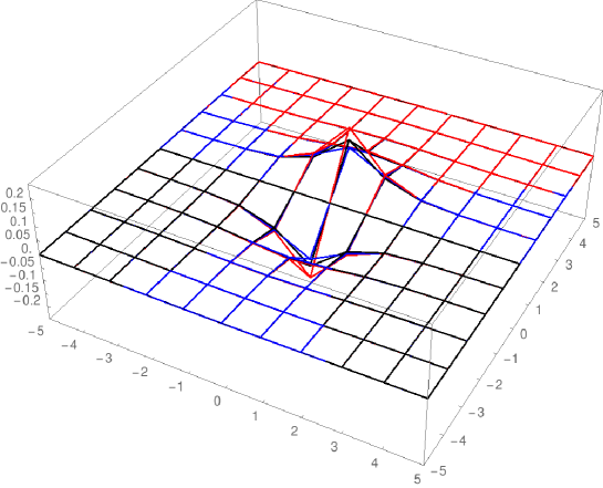
Figure 2. Values of the kernels of the three transforms: $K_{\mathbb{H}^{(1)}}(n_{1},n_{2})$ (red), $K_{\mathcal{R}^{(1)}}(n_{1},n_{2})$ (blue), and $K_{R_{\mathrm{dis}}^{(1)}}(n_{1},n_{2})$ (black) for $n_{1},n_{2}\in\{-5,-4,\ldots,5\}$.

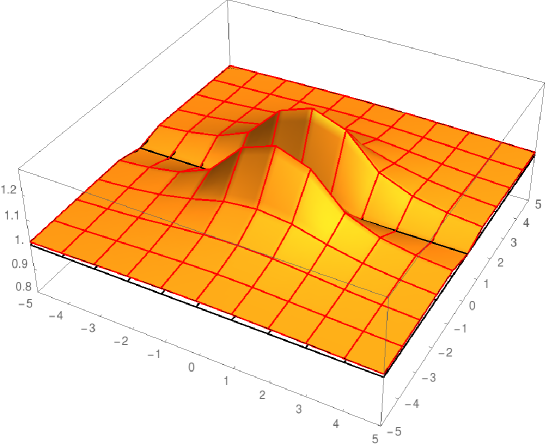
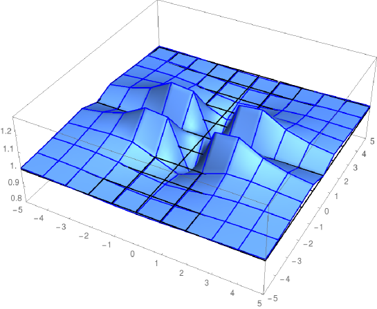
Figure 3. Ratio between the kernels of two transforms: $K_{\mathbb{H}^{(1)}}(n_{1},n_{2})/K_{R_{\mathrm{dis}}^{(1)}}(n_{1},n_{2})$ (red) compared with constant $1$ (black) for $n_{1},n_{2}\in\{-5,-4,\ldots,5\}$. When $n_{1}=0$, we set $0/0=1$.

Figure 4. Ratio between the kernels of two transforms: $K_{\mathcal{R}^{(1)}}(n_{1},n_{2})/K_{R_{\mathrm{dis}}^{(1)}}(n_{1},n_{2})$ (blue) compared with constant $1$ (black) for $n_{1},n_{2}\in\{-5,-4,\ldots,5\}$. When $n_{1}=0$, we set $0/0=1$.

The values of the three kernels are shown in Figure 2. Ratio between the kernels of the probabilistic and the CZ discrete Riesz transform are shown in Figure 4, while a similar plot for the method of rotations and the Riesz transform $R_{\mathrm{dis}}^{1}$ is shown in Figure 4. Numerical results are presented in Tables 1, 3 and 3.

Our simulations suggest that there is no general point-wise relation between the kernels of $\mathcal{R}^{(k)}$ and $R_{\mathrm{dis}}^{(k)}$, nor there is one between the kernels of $T_{\mathbb{H}^{(k)}}$ and $\mathcal{R}^{(k)}$. However, it seems that the kernel of $T_{\mathbb{H}^{(k)}}$ is always greater (in the absolute value) than the kernel of $R_{\mathrm{dis}}^{(k)}$. This leads to the following conjecture which we know is true for $d=1$ by (6.8).

Conjecture 10.1.

For all $d\geq 2$, we have $|K_{\mathbb{H}^{(k)}}(n)|\geq|K_{R_{\mathrm{dis}}^{(k)}}(n)|$ for every $n\in\mathbb{Z}^{d}$.

The above numerical findings give little insight into Question 7.7, which asks whether $K_{R_{\mathrm{dis}}^{(k)}}$ is the convolution of $K_{\mathbb{H}^{(k)}}$ with some probability kernel. Indeed, although intuitively point-wise domination asserted in Conjecture 10.1 appears to be a necessary condition for a positive answer to Question 7.7, neither of these statements implies the other one.

On the other hand, our calculations strongly suggest that in dimension $d=2$ the maximum of $K_{\mathcal{R}^{(1)}}(n_{1},n_{2})$ is strictly smaller than the maximum of $K_{R_{\mathrm{dis}}^{(1)}}(n_{1},n_{2})$; both maxima are attained at $(n_{1},n_{2})=(1,0)$. If this is indeed the case, then $K_{R_{\mathrm{dis}}^{(1)}}$ is clearly not a convolution of $K_{\mathcal{R}^{(1)}}$ and a probability kernel. Thus, we expect that the analogue of Question 7.7 for $\mathcal{R}^{(k)}$ instead of $T_{\mathbb{H}^{(k)}}$ has a negative answer.

Finally, one can ask if the analogue of Question 7.7 holds for the discrete Riesz transform obtained with the method of rotations, but using the probabilistic discrete Hilbert transform $T_{\mathbb{H}}$ instead of the usual discrete Hilbert transform $H_{\mathrm{dis}}$. We did not attempt to answer this question.

Table 1. Values of the kernels of the three transforms: $K_{\mathbb{H}^{(1)}}(n_{1},n_{2})$ (top row), $K_{\mathcal{R}^{(1)}}(n_{1},n_{2})$ (middle row) and $K_{R_{\mathrm{dis}}^{(1)}}(n_{1},n_{2})$ (bottom row) for $n_{1},n_{2}\in\{0,1,\ldots,5\}$, $n_{1}\neq 0$. The largest value in each cell is set in bold, while the smallest one is given in slanted type.

		$n_{2}$
		0	1	2	3	4	5
	1	0.2051 0.1318 0.1592	0.0698 0.0649 0.0563	0.0158 0.0166 0.0142	0.0053 0.0055 0.0050	0.0024 0.0024 0.0023	0.0012 0.0012 0.0012
	2	0.0446 0.0376 0.0398	0.0315 0.0284 0.0285	0.0151 0.0147 0.0141	0.0071 0.0071 0.0068	0.0037 0.0037 0.0036	0.0021 0.0021 0.0020
$n_{1}$	3	0.0188 0.0172 0.0177	0.0160 0.0149 0.0151	0.0106 0.0103 0.0102	0.0065 0.0064 0.0063	0.0039 0.0039 0.0038	0.0025 0.0025 0.0024
	4	0.0103 0.0098 0.0099	0.0094 0.0090 0.0091	0.0073 0.0071 0.0071	0.0052 0.0051 0.0051	0.0036 0.0036 0.0035	0.0025 0.0025 0.0024
	5	0.0065 0.0063 0.0064	0.0061 0.0060 0.0060	0.0052 0.0051 0.0051	0.0041 0.0040 0.0040	0.0031 0.0030 0.0030	0.0023 0.0023 0.0023

Table 2. Values of the ratios $K_{\mathbb{H}^{(1)}}(n_{1},n_{2})/K_{R_{\mathrm{dis}}^{(1)}}(n_{1},n_{2})$ of kernels of two transforms for $n_{1},n_{2}\in\{0,1,\ldots,5\}$, $n_{1}\neq 0$.

		$n_{2}$
		0	1	2	3	4	5
	1	1.2885	1.2413	1.1127	1.0593	1.0356	1.0235
	2	1.1200	1.1067	1.0717	1.0458	1.0303	1.0211
$n_{1}$	3	1.0615	1.0567	1.0450	1.0333	1.0243	1.0180
	4	1.0364	1.0345	1.0298	1.0241	1.0191	1.0150
	5	1.0239	1.0230	1.0208	1.0179	1.0149	1.0123

Table 3. Values of the ratios $K_{\mathcal{R}^{(1)}}(n_{1},n_{2})/K_{R_{\mathrm{dis}}^{(1)}}(n_{1},n_{2})$ of kernels of two transforms for $n_{1},n_{2}\in\{0,1,\ldots,5\}$, $n_{1}\neq 0$.

		$n_{2}$
		0	1	2	3	4	5
	1	0.8284	1.1530	1.1667	1.0947	1.0574	1.0379
	2	0.9443	0.9959	1.0452	1.0483	1.0385	1.0292
$n_{1}$	3	0.9737	0.9873	1.0094	1.0205	1.0221	1.0199
	4	0.9848	0.9897	0.9997	1.0077	1.0116	1.0125
	5	0.9902	0.9923	0.9972	1.0022	1.0057	1.0075

Acknowledgments

We thank Renming Song for conversation regarding positive-definite functions and for pointing out reference [Jacob1]. We thank Mark Ashbaugh for useful conversations on special functions. The research for this paper was conducted while the second author was a J. L. Doob research assistant professor at the University of Illinois at Urbana-Champaign.