Fast Ion Gates Outside the Lamb-Dicke Regime by Robust Quantum Optimal Control

Abstract

We present a robust quantum optimal control framework for implementing fast entangling gates on ion-trap quantum processors. The framework leverages tailored laser pulses to drive the multiple vibrational sidebands of the ions to create phonon-mediated entangling gates and, unlike the state of the art, requires neither weak-coupling Lamb-Dicke approximation nor perturbation treatment. With the application of gradient-based optimal control, it enables finding amplitude- and phase-modulated laser control protocols that work beyond the Lamb-Dicke regime, promising gate speed at the order of microseconds comparable to the characteristic trap frequencies. Also, robustness requirements on the temperature of the ions and initial optical phase can be conveniently included to pursue high-quality fast gates against experimental imperfections. Our approach represents a step in speeding up quantum gates to achieve larger quantum circuits for quantum computation and simulation, and thus can find applications in near-future experiments.

I Introduction

Trapped atomic ions are considered a rather promising platform for realizing large-scale quantum computers [1, 2, 3]. To bring this potential to reality, it is essential to perform fast, accurate, and robust entangling gates [4]. While high-fidelity single-qubit gates have been implemented and two-qubit gates have also steadily improved their precisions over the past decades [5, 6, 7, 8, 9], the time-efficiency of performing entangling gates remains exceedingly hard to scale faster. Current implementations of entangling gates typically cost tens to hundreds of microseconds [10, 11, 12], much slower than the speed limit set by the trap period of a few microseconds. The rather slow gate speed hence represents a limiting factor for reaching larger-sized quantum information processing experiments on ion-trap systems.

Entangling gates on trapped ions are realized through the mechanism of phonon-mediated qubit couplings, which is created by laser driving of the vibrational modes of the ions in the trap [13, 14, 15]. Most existing gate schemes essentially rely on the Lamb-Dicke approximation which assumes slow field driving and weak ion-motion interactions, and also on approximation technique of perturbation theory such as Magnus expansion. When increasing the gate speed, much stronger laser driving is needed, and the resulting larger displacements of the ions in phase space cause considerable deviations from the Lamb-Dicke regime. Accordingly, the previous approximations are no longer valid that, the higher-order error terms in evolution that have not been allowed for before now become prominent. This poses the major hindrance in constructing fast gates outside the Lamb-Dicke regime.

There have been considerable theoretical [16, 17, 18, 19, 20, 21, 22] and experimental [23, 24, 25] efforts to speed up ion gates, the attempts are challenging. For example, Ref. [24] reported a high-fidelity (99.8%) 1.6 $\mu$s gate and a much worse fidelity ($\sim$60%) 480 ns gate in experiments. The pulse synthesis method adopted there is still under the Lamb-Dicke condition, so the breakdown of Lamb-Dicke approximation comprises a major source of gate infidelity. Theoretically, there were proposals that take more Lamb-Dicke expansion terms into account [20, 22], but as higher-order sideband transitions are driven, it gets more complicated to derive the corresponding suitable driving profiles. Within the Lamb-Dicke regime, comparably simple driving schemes can be devised; outside the Lamb-Dicke regime, the nonlinearity inherent in the Hamiltonian makes the dynamical control problem less tractable. Moreover, the theoretical analysis can be even harder when one wants to add consideration of robustness to various noises.

In this work, we propose to use robust quantum optimal control (QOC) to tackle the problem of fast ion gates. QOC is a flexible and very effective method in finding high-performance pulses that accomplish given control tasks on a quantum system. Over the many years, it becomes a versatile tool in quantum technologies [26] and has found broad applications in diverse quantum platforms [27, 28, 29, 30, 31, 32]. In particular, QOC plays an important role in trapped-ions systems for devising and implementing amplitude, frequency or phase-modulated entangling gates [33, 34, 35, 36, 37], but usually being used in combination with Lamb-Dicke approximation and second-order Magnus expansion. Here, we show that, such approximations are unnecessary. We construct a general framework of QOC-based fast ion gates outside the Lamb-Dicke regime, which directly deals with the full dynamical evolution generated by the full Hamiltonian. The construction is exemplified on the Mølmer-Sørensen scheme [14], but should apply well to other similar gate schemes. Robustness requirements are also incorporated into QOC as either extra constraints on pulse parameters or additional optimization objectives. We then give a concrete two-qubit gate example with duration 3 $\mu$s, infidelity $<10^{-3}$ and insensitivity to initial optical phase, which demonstrates the applicability of our framework. We see that an advantage of fast gates is that they are less sensitive to errors associated with motional frequency dirfts or heating due to their significantly reduced gate time.

II Problem Description

Consider a single chain consisting of $N$ identical ions which are one-dimensionally aligned along $z$ axis; see Fig. 1(a). Qubits are encoded in a pair of internal energy levels belonging to each ion, while the whole ion chain vibrates collectively due to the long-range Coulomb repulsion. Therefore, the free Hamiltonian of the above system is ($\hbar=1$)

$$\hat{H}_{0}=\sum_{k=1}^{N}\omega_{q}\hat{\sigma}^{k}_{z}/2+\sum_{j=1}^{N}\nu_{j}\hat{a}_{j}^{\dagger}\hat{a}_{j}.$$ (1)

Here, $\omega_{q}$ denotes the energy gap of the encoded ion qubits, and $\hat{\sigma}_{x,y,z}^{k}$ are Pauli matrices for the $k$th qubit. For simplicity, we shall only consider the collective motional modes along the $z$ axis, and $\nu_{j}$ is the eigen-frequency of the $j$th mode with $\hat{a}_{j}^{\dagger}$ and $\hat{a}_{j}$ being the corresponding ladder operators. The ion qubits are conventionally coupled to the motional modes via laser-ion interactions. Individual addressing ability on each qubit is assumed in our general discussion, as illustrated in Fig. 1(a). Although this diagram considers hyperfine qubits manipulated via the two-photon stimulated Raman transitions, our approach is suitable for optical qubits as well.

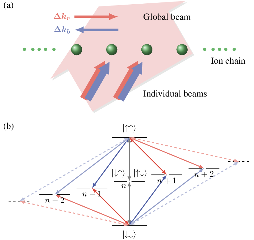
Figure 1: (a) Laser beam geometry in phase insensitive configuration. The wavevector differences for pairs of frequencies driving the red sideband and the blue sideband travel in the opposite direction. (b) Illustration of multi-sideband driving protocol under the Mølmer-Sørensen gate scheme. Qubits are stored in the hyperfine states of the ions denoted by $\left|\uparrow\right\rangle$ and $\left|\uparrow\right\rangle$, and the motional state is characterized by the phonon number $n$. Outside the Lamb-Dicke regime, higher-order blue and red sideband transitions are also excited simultaneously.

We now describe the widely used Mølmer-Sørensen [14, 38] gate scheme. In its basic form, it requires bichromatic laser fields with frequencies of $\omega_{q}\pm\omega$ to illuminate targeted ions and simultaneously induce the first blue and red sideband transitions. We here assume the phase-insensitive configuration of the bichromatic fields, where the effective wave vectors for the two sidebands ($\Delta\bm{k}_{b}=-\Delta\bm{k}_{r}=\bm{k}$) propagate in opposite directions [39, 22]. As a result, we can obtain the following expression for the laser-ion interaction Hamiltonian in the ions’ resonant rotating frame

$$\hat{H}_{C}(t)=\sum_{k=1}^{N}\dfrac{\Omega}{2}\left[e^{i\left(-\bm{k}z_{k}-\omega t+\phi_{r}\right)}+e^{i\left(\bm{k}z_{k}+\omega t+\phi_{b}\right)}\right]\hat{\sigma}_{+}^{k}+\text{h.c.}$$ (2)

Here, the effective laser-ion coupling strengths for the both sideband transitions are balanced to an equal value of $\Omega$, while $\phi_{b}$ and $\phi_{r}$ represent the independent optical phase for the blue and red sideband, respectively. If we further define the so-named spin phase $\phi=(\phi_{b}+\phi_{r})/2$ and the motional phase $\varphi=(\phi_{b}-\phi_{r})/2$ [39], the above equation can be rewritten as

$$\hat{H}_{C}(t)=\sum_{k=1}^{N}\Omega\hat{\sigma}^{k}_{\phi_{S}}\cos{\left(\omega t+\varphi+\bm{k}z_{k}\right)},$$ (3)

where $\hat{\sigma}_{\phi}=\hat{\sigma}_{x}\cos\phi+\hat{\sigma}_{y}\sin\phi$. Note that, the pulse parameters of $\{\Omega,\phi,\varphi\}$ can be site-dependent if one of the beams to drive the Raman transitions has the ability of individual addressing. The position operator $z_{k}$ can be expanded into the linear combination of the operators of the collective motion as $z_{k}=\sum_{j}b_{kj}\Delta z_{j}(\hat{a}_{j}+\hat{a}_{j}^{\dagger})$, where $\Delta z_{j}=\sqrt{\hbar/2M\nu_{j}}$ is the size of the ground-state wavepacket of the $j$th motional mode, and ${b_{kj}}$ is the normal-mode transformation matrix. Conventionally, we denote the coefficient $b_{kj}\bm{k}\Delta z_{j}$ by $\eta_{kj}$, which are referred to as the Lamb-Dicke parameters. Accordingly, the control Hamiltonian can be further expressed as

$$\hat{H}_{C}(t)=\sum_{k=1}^{N}\Omega\hat{\sigma}_{\phi}^{k}\cos{\left[\omega t+\varphi+\sum_{j=1}^{N}\eta_{kj}(\hat{a}_{j}+\hat{a}_{j}^{\dagger})\right]}.$$ (4)

If the ions are sufficiently cooled and the spatial motion keeps small, so that the condition for the Lamb-Dicke regime is met, then the laser-ion interaction Hamiltonian admits a simplified form by taking the approximation $e^{i\eta(\hat{a}+\hat{a}^{\dagger})}\approx 1+i\eta(\hat{a}+\hat{a}^{\dagger})$. This is the normal way to simplify treatments of laser driven ion dynamics. Most of the currently employed entangling gates operate in the Lamb-Dicke regime.

To go beyond the Lamb-Dicke regime, it is desirable to excite the higher-order sideband transitions. Hence we would like to use multichromatic laser beam to address the multiple sidebands simultaneously; see an illustration in Fig. 1(b). Such a driving protocol was previously used to generate robust gates against different sources of noises [40, 41]. For the present problem, we assume that the multichromatic laser beam contains $L$ frequency pairs $\{\pm\omega_{l}:l=1,...,L\}$, and for the $l$th frequency component, its corresponding amplitude, spin phase and motional phase modulations are denoted by $\Omega_{l}(t)$, $\phi_{l}(t)$ and $\varphi_{l}(t)$, respectively. Similar to the previous derivations, the control Hamiltonian now has the form

$$\hat{H}_{C}=\sum_{k=1}^{N}\sum_{l=1}^{L}\Omega_{l}\hat{\sigma}_{\phi_{l}}^{k}\cos\left[\omega_{l}t+\varphi_{l}+\sum_{j=1}^{N}\eta_{kj}(\hat{a}_{j}+\hat{a}_{j}^{\dagger})\right].$$

We point out that, although we assume predefined driving frequencies in this work, our method can apply as well to continuous frequency modulation in which the pulse frequency serves as optimization parameters.

Our goal is to perform a target quantum gate $\hat{\overline{U}}$, which is a unitary transformation on the computational states namely the internal states. The task is hence to find a shaped control pulse determined by a set of real-valued functions $\{\Omega_{l}(t),\phi_{l}(t),\varphi_{l}(t)\}$ such that, the time propagator at the end of the evolution implements $\hat{\overline{U}}$ on the ions’ internal state, but meanwhile should not change the ions’ external state. If the ions can be perfectly cooled, we can assume the ions are initially at the vibrational ground state. But this is a difficult condition. More realistically, the motional state is at a statistical mixture. In this work, we shall suppose that the ions’ vibrational modes are initially in the thermal product state $\hat{\rho}_{\text{th}}=\hat{\rho}^{1}_{\text{th}}\otimes\hat{\rho}^{2}_{\text{th}}\otimes\cdots\otimes\hat{\rho}^{N}_{\text{th}}$ with

$$\hat{\rho}^{j}_{\text{th}}=\left(1-e^{-\nu_{j}/k_{B}T}\right)\sum_{n\geq 0}|n\rangle\langle n|e^{-n\nu_{j}/k_{B}T}$$

for $j=1,...,N$, where $k_{B}$ is the Boltzmann constant and $T$ represents the temperature. Recall that the Lamb-Dicke regime refers to the situation where the spatial spread of the wave-function of the ions is much smaller than the wavelength of the laser field, or in mathematical words, $\eta\sqrt{\bar{n}+1}\ll 1$ where $\bar{n}$ is the average phonon occupation number. But to implement fast gates, strong laser driving is necessary, and the ion motion may be considerably excited during the evolution, so the Lamb-Dicke approximation would no longer be valid. Besides, to avoid imposing stringent requirements on ion cooling, we would like our optimal control scheme be effective without necessarily assuming negligible initial average occupation $\bar{n}$.

III Quantum Optimal Control

In this section, we shall formulate the quantum optimal control problem for the task of fast ion gate outside the Lamb-Dicke regime, and describe how to solve the problem by using gradient-based methods.

III.1 System and Control

As the first step, we make clear the system Hamiltonian and the control Hamiltonian. In the ions’ resonant rotating frame, the system Hamiltonian goes

$$\hat{H}_{S}=\sum_{j=1}^{N}\nu_{j}\hat{a}_{j}^{\dagger}\hat{a}_{j},$$ (5)

and the control Hamiltonian can be written as

$$\hat{H}_{C} =\sum_{k=1}^{N}\sum_{l=1}^{L}\Omega_{l}\hat{\sigma}_{\phi_{l}}^{k}\cos\left[\omega_{l}t+\varphi_{l}+\sum_{j=1}^{N}\eta_{kj}(\hat{a}_{j}+\hat{a}_{j}^{\dagger})\right]$$

$$=\sum_{k=1}^{N}\sum_{l=1}^{L}\Omega_{l}\hat{\sigma}_{\phi_{l}}^{k}\left[\cos(\omega_{l}t+\varphi_{l})\hat{\xi}^{k}_{x}+\sin(\omega_{l}t+\varphi_{l})\hat{\xi}^{k}_{y}\right],$$

where

$$\hat{\xi}^{k}_{1} =\cos\left[\sum_{j=1}^{N}\eta_{kj}(\hat{a}_{j}+\hat{a}_{j}^{\dagger})\right],$$

$$\hat{\xi}^{k}_{2} =-\sin\left[\sum_{j=1}^{N}\eta_{kj}(\hat{a}_{j}+\hat{a}_{j}^{\dagger})\right].$$

To simplify the notations in our subsequent derivations, we define $\hat{\xi}^{k}_{\omega_{l}t+\varphi_{l}}=\cos(\omega_{l}t+\varphi_{l})\hat{\xi}^{k}_{1}+\sin(\omega_{l}t+\varphi_{l})\hat{\xi}^{k}_{2}$, then

$$\hat{H}_{C}=\sum_{k=1}^{N}\sum_{l=1}^{L}\Omega_{l}\hat{\sigma}_{\phi_{l}}^{k}\hat{\xi}^{k}_{\omega_{l}t+\varphi_{l}}.$$ (6)

Assume that the laser pulse has time length $T$, then the combined evolution of $H_{S}+H_{C}(t)$ results in the time evolution operator

$$\hat{U}(T)=\mathcal{T}\exp\left(-i\int_{0}^{T}dt[\hat{H}_{S}+\hat{H}_{C}(t)]\right),$$ (7)

where $\mathcal{T}$ denotes the time ordering operation. Since our approach no longer takes the Lamb-Dicke approximation of any order, all the nonlinear dependence of $\hat{H}_{C}$ on the phonon creation and annihilation operators will contribute to the controlled evolution.

III.2 Average Gate Fidelity

In quantum optimal control, normally we define an objective function to measure the control performance. Note that, while $\hat{U}(t)$ is unitary in the whole state space, it generates a quantum channel in the subspace of internal states. How well this channel realizes the target gate can be quantitatively characterized through the average gate fidelity function, which we describe as follows. Suppose the initial input internal state of the ions is $|\psi\rangle\langle\psi|$, suppose the ions are initially at the thermal state $\rho_{\text{th}}$, then at the end of the controlled evolution the actual output internal state is given by $\hat{\rho}=\operatorname{Tr}_{\text{m}}\left[\hat{U}(T)|\psi\rangle\langle\psi|\otimes\hat{\rho}_{\text{th}}\hat{U}^{\dagger}(T)\right]$, where $\operatorname{Tr}_{\text{m}}$ means taking partial trace over the external degrees of freedom. The similarity between $\hat{\rho}$ and the ideal state $\hat{\overline{U}}|\psi\rangle$ can be estimated by the state fidelity $\langle\psi|\hat{\overline{U}}^{\dagger}\hat{\rho}\overline{U}|\psi\rangle$. To compare $\hat{U}(T)$ and $\hat{\overline{U}}$, we need a state-independent measure which serves as our fitness function, that is, the average gate fidelity, defined by

$$f=\int d\psi\langle\psi|\hat{\overline{U}}^{\dagger}\operatorname{Tr}_{\text{m}}[\hat{U}(T)|\psi\rangle\langle\psi|\otimes\hat{\rho}_{\text{th}}\hat{U}^{\dagger}(T)]\hat{\overline{U}}|\psi\rangle,$$ (8)

where the integration is taken over the uniform (Haar) measure $d\psi$ on the internal state space. A simple expression for computing the average gate fidelity is the following [42]

$$f=\frac{\sum_{i}\operatorname{Tr}\left\{\hat{\overline{U}}\hat{P}_{i}^{\dagger}\hat{\overline{U}}^{\dagger}\operatorname{Tr}_{\text{m}}\left[\hat{U}(T)\hat{P}_{i}\otimes\hat{\rho}_{\text{th}}\hat{U}^{\dagger}(T)\right]\right\}+d^{2}}{d^{2}(d+1)},$$ (9)

where $d=2^{N}$ and $\{\hat{P}_{i}\}$ is an orthogonal basis of $d\times d$ unitary operators such that $\operatorname{Tr}[\hat{P}_{i}^{\dagger}\hat{P}_{j}]=\delta_{ij}d$. Here, we would choose the Pauli operators $\{\hat{P}_{i}\}=\{I,\hat{\sigma}_{x},\hat{\sigma}_{y},\hat{\sigma}_{z}\}^{\otimes N}$, where $I$ is the identity operator.

At this point, we are ready to formally state the quantum optimal control problem for target gate realization: we set a suitable choice of the laser driving frequencies $\{\omega_{l}\}$, and

find $$\{\Omega_{l}(t),\phi_{l}(t),\varphi_{l}(t)\},$$

$$\max\quad f(\hat{U}(T),\hat{\overline{U}}),\$$

s.t. $$\frac{\partial\hat{U}(t)}{\partial t}=-i[\hat{H}_{S}+\hat{H}_{C}(t)]\hat{U}(t).$$

III.3 Gradient-based Optimization

In general, it is difficult to construct analytic optimal control solutions, so taking numerical approach is necessary. The GRAPE algorithm [27] is one widely used numerical optimization technique for solving optimal control problems. In the following, we outline its basics.

First, we should discretize the controlled evolution. Let the evolution be divided into $M$ slices of equal length $\tau=T/M$, and in each time slice the control is time-invariant. The time discretization $\tau$ is naturally given by the time resolution of the lasers generating the pulse. We represent the set of pulse parameters after discretization by an array $\bm{u}=(\bm{\Omega},\bm{\phi},\bm{\varphi})$, where $\bm{\Omega}=(\Omega_{lm})$, $\bm{\phi}=(\phi_{lm})$ and $\bm{\varphi}=(\varphi_{lm})$ are arrays of pulse parameters all of size $L\times M$, with their $lm$th elements corresponding to the amplitude, spin phase and motional phase of the $l$th frequency component of the pulse at the $m$th time slice, respectively. Provided that $\tau$ is small, we can view the control Hamiltonian as constant in each slice. Let $\hat{H}_{C}[m]$ denote the control Hamiltonian at the $m$th slice, and $\hat{U}_{m}=\exp\left\{-i\tau(\hat{H}_{S}+\hat{H}_{C}[m])\right\}$ the corresponding time evolution operator, then the total time evolution operator is given by $\hat{U}(T)=\hat{U}_{M}\cdots\hat{U}_{1}$.

To seek an optimal pulse solution, the GRAPE algorithm starts from an initial pulse guess $\bm{u}^{(0)}$, and generates a sequence of iterates $\bm{u}^{(1)},\bm{u}^{(2)},...,$ by taking steps along the gradient ascent direction

$$\bm{u}^{(k+1)}=\bm{u}^{(k)}+\alpha^{(k)}\bm{g}^{(k)},$$ (10)

where $\bm{g}^{(k)}$ is the gradient of the target function $f$ at the $k$th iterate $\bm{u}^{(k)}$, and $\alpha^{(k)}$ is a step size chosen such that an adequate increase in $f$ along $\bm{g}^{(k)}$ can be acquired. The gradient $\bm{g}$ of $f$ with respect to the control parameters can be evaluated according to

$$\bm{g}=\frac{\sum\limits_{i}\operatorname{Tr}\left\{\hat{\overline{U}}\hat{P}_{i}^{\dagger}\hat{\overline{U}}^{\dagger}\operatorname{Tr}_{\text{m}}\left[\displaystyle\frac{\partial\hat{U}}{\partial\bm{u}}\hat{P}_{i}\otimes\hat{\rho}_{\text{th}}\hat{U}^{\dagger}+\text{h.c.}\right]\right\}}{d^{2}(d+1)},$$ (11)

where $\partial\hat{U}/\partial\bm{u}=(\partial\hat{U}/\partial\bm{\Omega},\partial\hat{U}/\partial\bm{\phi},\partial\hat{U}/\partial\bm{\varphi})$. Assuming that the discretization step $\tau$ is small, and let $u[m]$ denote any of the control parameters at the $m$th slice evolution, there is

$$\frac{\partial\hat{U}}{\partial u[m]} =\hat{U}_{M}\cdots\frac{\partial\hat{U}_{m}}{\partial u[m]}\cdots\hat{U}_{1}$$

$$=\hat{U}_{M}\cdots\left(-i\tau\frac{\partial\hat{H}_{C}[m]}{\partial u[m]}\hat{U}_{m}\right)\cdots\hat{U}_{1}+O(\tau^{2}).$$ (12)

Then, from Eq. (6) we have that

$$\frac{\partial\hat{H}_{C}[m]}{\partial\Omega_{lm}} =\sum_{k=1}^{N}\hat{\sigma}_{\phi_{lm}}^{k}\hat{\xi}^{k}_{\omega_{l}m\tau+\varphi_{lm}},$$ (13a)

$$\frac{\partial\hat{H}_{C}[m]}{\partial\phi_{lm}} =\sum_{k=1}^{N}\Omega_{lm}\hat{\sigma}_{\phi_{lm}+\pi/2}^{k}\hat{\xi}^{k}_{\omega_{l}m\tau+\varphi_{lm}},$$ (13b)

$$\frac{\partial\hat{H}_{C}[m]}{\partial\varphi_{lm}} =\sum_{k=1}^{N}\Omega_{lm}\hat{\sigma}_{\phi_{lm}}^{k}\hat{\xi}^{k}_{\omega_{l}m\tau+\varphi_{lm}+\pi/2}.$$ (13c)

Hence, Eqs. (11), (12) and (13) together provides an explicit way of gradient evaluation.

In the practice of GRAPE, some important considerations need be made clear as below.

Smoothness consideration. Real waveform generators have finite response times. To avoid sharp edges as is the problem for rectangular pulses, we could restrict to consider the following class of pulses using truncated Fourier basis

$$\Omega(t)=\sum_{k=1}^{k_{\max}}c_{k}\left[1-\cos(2\pi kt/T)\right].$$ (14)

Apparently, pulse waveforms thus specified automatically goes smoothly to zero at the beginning and end of the pulse. Another simple strategy is to use a lowpass filter to suppress the high-frequency components in the pulse waveform after each iteration and also, the gradient needs be filtered as well.

Accuracy in gradient estimation. For sufficiently small $\tau$, it suffices to take the first-order approximation in the expression Eq. (12) for computing $\bm{g}$. It is also possible to allow for the higher order terms to get more accurate estimation of $\bm{g}$ [43], which we will not brief here.

Convergence speed. Since GRAPE utilizes only first-order gradient information, it actually has a linear convergence speed. Faster convergence can be achieved if one also takes into account of higher-order gradients. For example, conjugated gradient or quasi-Newton methods combine first- and second-order gradient information to determine a suitable gradient-related search direction, and thus can provide superlinear convergence speed. Such methods have been introduced and practiced in quantum optimal control, resulting in some improved variants of GRAPE [44, 43]. Interested readers are referred to standard books on numerical optimization such as Ref. [45] for more details.

III.4 Initial Phase Robustness

The above optimization presumes that we can control and stabilize the laser phases, which is however not that true in real experiments. Specifically, in the phase-insensitive configuration considered here, there would exist an unpredictable initial motional phase $\varphi_{0}]$. This means that the actual evolution is driven by the control Hamiltonian $\hat{H}_{C}(\Omega,\phi,\varphi+\varphi_{0})$ rather than $\hat{H}_{C}(\Omega,\phi,\varphi)$. To address the issue, it is required that the optimal pulse should be robust to $\varphi_{0}$ over the entire range $[0,2\pi]$.

Our consideration of initial phase robustness consists of two steps. First, we sample a set of different initial optical phases $\{\varphi^{s}_{0}\in[0,2\pi]\}$ and compute their corresponding gate fidelities $\{f_{\varphi^{s}_{0}}\}$, here $s=1,..,S$ with $S$ the number of samples. It is natural to use the average of the gate fidelities over the sampled initial phases $\frac{1}{S}\sum_{s=1}^{S}f_{\varphi^{s}_{0}}$ as the new objective function. Next, we further require that the controlled evolution has first-order robustness property with respect to $\varphi_{0}$ at the points of the sampled phases.

We remark that both steps are important. If we only use sampling, the obvious drawback is that we can only make the fidelity optimal at the sampled phases, while for the other unsampled phases the fidelity could very likely be still low. On the other hand, if we only employ robust control, it is necessary to involve complicated higher-order perturbation theory to ensure that the robustness region can cover the entire region $[0,2\pi]$. Therefore, we are inclined to combining both techniques to achieve smooth, wide-range pulse robustness.

The sampling-based optimization step is quite straightforward. Now, we describe how to incorporate first-order robustness into optimal control. As illustration, we consider $\varphi_{0}$ robustness at $\varphi_{0}=0$. Suppose there is a small perturbation $\delta\varphi$, the control Hamiltonian becomes

$$\hat{H}_{C} =\sum_{k=1}^{N}\sum_{l=1}^{L}\Omega_{l}\hat{\sigma}_{\phi_{l}}^{k}\hat{\xi}^{k}_{\omega_{l}t+\varphi_{l}+\delta\varphi}$$

$$=\sum_{k=1}^{N}\sum_{l=1}^{L}\Omega_{l}\hat{\sigma}_{\phi_{l}}^{k}(\hat{\xi}^{k}_{\omega_{l}t+\varphi_{l}}+\delta\varphi\hat{\xi}^{k}_{\omega_{l}t+\varphi_{l}+\pi/2}+O(\delta\varphi^{2})).$$

Hence, to first-order approximation the perturbed Hamiltonian is

$$\hat{H}_{S}+\hat{H}_{C}(t)+\delta\varphi\hat{H}^{\prime}(t),$$ (15)

where we define

$$\hat{H}^{\prime}(t)=\sum_{k=1}^{N}\sum_{l=1}^{L}\Omega_{l}\hat{\sigma}_{\phi_{l}}^{k}\hat{\xi}^{k}_{\omega_{l}t+\varphi_{l}+\pi/2}$$

as the perturbation operator. Without perturbation, the system evolution is given by $\hat{U}(t)$ as before; in the presence of perturbation, the real evolution $\hat{U}_{\text{real}}(t)$ deviates from the ideal $\hat{U}(t)$, and the deviation can be characterized by the Dyson series [46] $\hat{U}_{\text{real}}(t)=\hat{U}(t)+\hat{U}_{\text{err}}^{(1)}(t)+\cdots$. Here, we shall only keep the first-order error term $U_{\text{err}}^{(1)}(t)$, which has the expression

$$\hat{U}_{\text{err}}^{(1)}(t)=-i\hat{U}(t)\int_{0}^{t}dt_{1}\hat{U}^{\dagger}(t_{1})\delta\varphi\hat{H}^{\prime}(t_{1})\hat{U}(t_{1}).$$ (16)

One can introduce the definition

$$\mathcal{D}_{\hat{U}(t)}(\hat{H}^{\prime}(t)) =\frac{\hat{U}_{\text{real}}(t)-\hat{U}(t)}{\delta\varphi}$$

$$=-i\hat{U}(t)\int_{0}^{t}dt_{1}\hat{U}^{\dagger}(t_{1})\hat{H}^{\prime}(t_{1})\hat{U}(t_{1}).$$

It captures the first-order perturbative effect in the evolution operator $\hat{U}(t)$ due to the presence of $\hat{H}^{\prime}(t)$, and is referred to as the directional derivative of $\hat{U}(t)$ along $\hat{H}^{\prime}(t)$ in Ref. [47]. Therefore, minimizing the magnitude of $\mathcal{D}_{\hat{U}(t)}(\hat{H}^{\prime}(t))$ would imply that even there is a small phase variation $\delta\varphi$, the actual evolution is still close to the ideal one. Ref. [47] also provides a very effective way to compute $\mathcal{D}_{\hat{U}(t)}(\hat{H}^{\prime}(t))$ and its gradient, based on the technique of Van Loan matrix integral.

IV Two-qubit Example

Now, we give an explicit two-qubit gate example to show the effectiveness of our method. We consider two ¹⁷¹Yb⁺ ions in a trap frequency of $\nu_{z}=2\pi\times 1$MHz along $z$-axis [48]; therefore, the motional frequencies of the ion-chain turn out to be $\nu_{1}=\nu_{z}$ and $\nu_{2}=\sqrt{3}\nu_{z}$ for the center-of-mass mode and stretching mode, respectively. The ion qubit is encoded in the hyperfine clock state in the ground manifold and then manipulated via 355 nm lasers [32, 34, 49], giving the Lamb-Dicke parameter around $0.136$ for the center-of-mass mode.

The target gate that we consider in our numerical tests is the maximally entangling gate $\hat{U}_{XX}=\exp\left(i\pi\sigma_{1}^{x}\sigma_{2}^{x}/4\right)$ for the internal degrees of freedom. Our driving protocol can be targeted at the sidebands of either the center-of-mass mode or the stretching mode, though the other mode would also be partially excited as we are in the fast gate regime. For simplicity, we shall consider amplitude-modulation only, with all spin phases and motional phases set to zero.

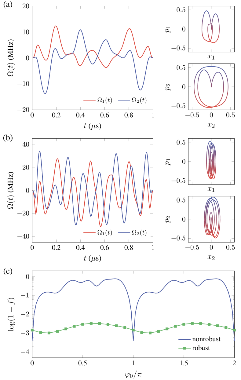
Figure 2: Optimal laser control pulses for the entangling gate $\hat{U}_{XX}$ with gate time $T=1$ $\mu$s and time step $\tau=5$ ns, under the ideal condition of perfect cooling $\bar{n}_{1}=\bar{n}_{2}=0$. (a) An optimal pulse solution of fidelity 0.9996, under the assumption that all phases are stabilized at zero. (b) A robust optimal pulse that is insensitive to initial phase instability, having phase-averaged gate fidelity $\sim 0.9979$. All the time-dependent amplitude shapes start and end smoothly at zero. Negative amplitudes correspond to an inversion of their corresponding spin phases. (c) Performance comparison of the two pulses in (a) and (b) in terms of initial phase robustness.

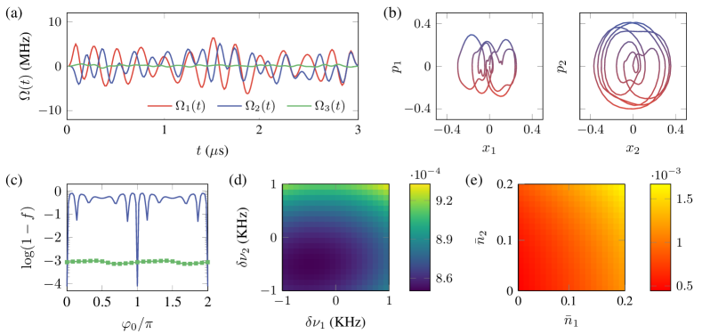
Figure 3: Optimal laser control pulse for the entangling gate $\hat{U}_{XX}$ with gate time $T=3$ $\mu$s and time step $\tau=15$ ns, under the condition of initial thermal occupation $\bar{n}_{1}=\bar{n}_{2}=0.1$. (a) Pulse shapes. The $l$th time-varying shape $\Omega_{l}(t)$ represents the amplitude modulation corresponding to the frequency component $\omega_{l}=l\nu_{2}$ for $l=1,2,3$. (b) Phase-space trajectories. These are overlapping at zero, indicating no residual state-motional entanglement. (c) Initial phase robustness. (d) Robustness profile with respect to normal-mode frequency errors. (e) Robustness profile with respect to initial thermal occupation.

IV.1 1 $\mu$s-gate

We study the case of gate time $T=1$ $\mu$s at the start, which corresponds to one vibrational period of the center of mass mode $1/\nu_{1}$. We first assume pulse control under ideal conditions that the ions’ motion is cooled perfectly, the pulse amplitudes can be arbitrarily large, and pulse phases can be made stable. Figure 2(a) shows a typical result of our obtained optimal pulse for implementing $\hat{U}_{XX}$, which achieves an average gate fidelity of 0.9996. It has two pairs of frequencies $\{\pm\omega_{l}:\omega_{l}=l\nu_{1};l=1,2\}$, as we find that using a single pair of frequencies is not sufficient to get a high fidelity. This is reasonable, since in the fast gate regime the Lamb-Dicke approximation is no longer valid, so it is needed to excite the higher-order sidebands. To show that our pulse indeed does not induce residual qubit-motion entanglement at the conclusion of the control operation, we plot the phase-space displacements of the two motional modes during the operation; see Fig. 2(b). The phase-space trajectories are calculated via

$$x_{j}(t) =\operatorname{Tr}\left({\hat{\rho}(t)\left|\psi_{j}\right\rangle\left\langle\psi_{j}\right|\otimes\hat{x}_{j}}\right),$$

$$p_{j}(t) =\operatorname{Tr}\left({\hat{\rho}(t)\left|\psi_{j}\right\rangle\left\langle\psi_{j}\right|\otimes\hat{p}_{j}}\right),$$

where $|\psi_{j}\rangle$ is $\left|++\right\rangle$ for mode $j=1$ or $\left|+-\right\rangle$ for mode $j=2$, $\hat{x}=(\hat{a}+\hat{a}^{\dagger})$ and $\hat{p}=i(\hat{a}-\hat{a}^{\dagger})$, $\hat{\rho}(t)$ is the state of the total system at time $t$ with the initial state being $\left|\uparrow\uparrow\right\rangle\left\langle\uparrow\uparrow\right|\otimes\hat{\rho}_{\text{th}}$.

Next, we consider robustness to initial phase $\varphi_{0}$ in our pulse search procedure. We choose four samples $\varphi_{0}\in\{0,\pi/4,\pi/2,3\pi/4\}$ and perform optimization such that the gate fidelity averaged over these samples is as high as possible. An optimal pulse solution is given in Fig. 2 (b), which achieves fidelity $\sim 0.9979$. It has larger amplitudes, and the resulting phase space trajectories are more complex. Fig. 2(c) compares initial phase robustness of the robust pulse and the previous one. We can see that robustness has indeed been substantially improved, but at the cost of some infidelity increase.

Our numerically found two optimal pulse solutions have maximum strength reaching a few tens of MHz. In practice, however, such pulses may be not experimentally friendly. It seems hard to find better performance 1 $\mu$s pulses, hence to make further improvements, we need to increase the pulse length.

IV.2 3 $\mu$s-gate

In order to lower the overall laser intensity, we set a longer pulse time $T=3$ $\mu$s and perform pulse search under realistic experimental conditions. Concretely, we assume that the initial thermal state $\hat{\rho}_{\text{th}}$ for the two motional modes has average occupation of $\bar{n}_{1}=0.1$ and $\bar{n}_{2}=0.1$, which is well within experimental capability. Robustness to initial phase $\varphi_{0}$ is also required. Figure 3 shows a result of our obtained robust optimal pulse, which achieves an average gate fidelity of 0.9991. Figure 3(c) compares initial phase robustness performances between pulses before and after robustness optimization. We also evaluate the robustness of the gate with respect to drifts in the two motional mode frequencies, finding that the pulse can suppress errors in gate fidelities to below $1\times 10^{-4}$ for up to a $\pm 1$ KHz frequency offset. In Fig. 3(e), we plot the gate infidelity with respect to the initial thermal occupation $\bar{n}_{1}$ and $\bar{n}_{2}$. It can be seen that, as the average phonon number increases from 0 to 0.2, the infidelity increases from $4.4\times 10^{-4}$ to $1.7\times 10^{-3}$ at an approximately linear rate. In summary, the optimal pulse is smooth, robust, and has amplitudes not exceeding 7 MHz, thus can be friendly to experimental implementation.

V Conclusion and Outlook

QOC is powerful for designing shaped pulses to induce target quantum operations. The idea of employing QOC for realizing fast entangling gates on trapped-ions system is simple and direct, but was not yet explored. The reason might be that the laser-ion interaction Hamiltonian in the fast gate regime has strong nonlinearity, which looks not easy to deal with. Our developed framework here allows for conveniently pursue high-quality shaped optical fields to drive the ions in the nonlinear regime. It remarkably does not depend on the assumption of Lamb-Dicke approximation, nor the application of average Hamiltonian theory. Through numerical tests on the case of two-qubit fast gate, we learned that: in ideal conditions, accurate and fast gates within one period of the trap frequency do exist, which suggests the speed limit to quantum processing with ions; but to meet current experimental requirements, longer pulses are necessary. Our results of $1$ $\mu$s- and $3$ $\mu$s-gates indicate that as the gate time increases, higher-fidelity and lower-intensity optimal pulse can be found. As a further example, if we increase the gate time to $5$ $\mu$s, we can achieve phase-insensitive gates of fidelity above 0.9999 with pulse amplitudes below 5 MHz. Therefore, it is to the experimenters’ choice to decide which of the following, gate speed, fidelity, phase robustness and other factors, are the most important considerations in real experiments.

The generic method introduced here may potentially advance small-sized trapped ion systems toward a new level of gate speed as well as precision. As for larger-sized systems, however, there is one important yet challenging problem. That is, QOC suffers from the intrinsic scalability issue. As the number of ion qubits grows, the system dimension grows exponentially, so it will require huge amount of computational resources to simulate the full controlled dynamics. Therefore, future work should place greater focus on improving the simulation efficiency. To give an example, we mention a software library introduced in Ref. [50], that trying to construct accurate low-dimensional matrix representations to replace the full evolution operators, and hence allows pulse search on large spin systems of as many as 40 spins with relative ease just on a desktop workstation. Our framework could incorporate similar strategies so as to extend to, e.g., long ion chains. Finally, the present framework is not limited to quantum gate implementation, but can also be applied to other quantum information processing tasks, which is worth further investigation. We anticipate that the systematic method proposed in this work can find experimental implementations as well as more quantum technology applications.

VI Acknowledgments

We acknowledge support by the National Natural Science Foundation of China (Grants No. 1212200199, 11975117, 12004165, 92065111, and 12204230), Guangdong Basic and Applied Basic Research Foundation (Grant No. 2021B1515020070), Guangdong Provincial Key Laboratory (Grant No. 2019B121203002), and Shenzhen Science and Technology Program (Grants No. RCYX20200714114522109, RCBS20200714114820298, and KQTD20200820113010023). Y.L. was supported by the National Natural Science Foundation of China (Grants No. 92165206, No. 11974330), Innovation Program for Quantum Science and Technology (Grant No. 2021ZD0301603), and the Fundamental Research Funds for the Central Universities.

References

- Häffner et al. [2008] H. Häffner, C. Roos, and R. Blatt, Quantum computing with trapped ions, Phys. Rep. 469, 155 (2008).
- Monroe and Kim [2013] C. Monroe and J. Kim, Scaling the ion trap quantum processor, Science 339, 1164 (2013).
- Bruzewicz et al. [2019] C. D. Bruzewicz, J. Chiaverini, R. McConnell, and J. M. Sage, Trapped-ion quantum computing: Progress and challenges, Appl. Phys. Rev. 6, 021314 (2019).
- DiVincenzo [2000] D. P. DiVincenzo, The Physical Implementation of Quantum Computation, Fortschr. Phys. 48, 771 (2000).
- Ballance et al. [2016] C. J. Ballance, T. P. Harty, N. M. Linke, M. A. Sepiol, and D. M. Lucas, High-Fidelity Quantum Logic Gates Using Trapped-Ion Hyperfine Qubits, Phys. Rev. Lett. 117, 060504 (2016).
- Gaebler et al. [2016] J. P. Gaebler, T. R. Tan, Y. Lin, Y. Wan, R. Bowler, A. C. Keith, S. Glancy, K. Coakley, E. Knill, D. Leibfried, and D. J. Wineland, High-Fidelity Universal Gate Set for Ion Qubits, Phys. Rev. Lett. 117, 060505 (2016).
- Wang et al. [2020] Y. Wang, S. Crain, C. Fang, B. Zhang, S. Huang, Q. Liang, P. H. Leung, K. R. Brown, and J. Kim, High-Fidelity Two-Qubit Gates Using a Microelectromechanical-System-Based Beam Steering System for Individual Qubit Addressing, Phys. Rev. Lett. 125, 150505 (2020).
- Clark et al. [2021] C. R. Clark, H. N. Tinkey, B. C. Sawyer, A. M. Meier, K. A. Burkhardt, C. M. Seck, C. M. Shappert, N. D. Guise, C. E. Volin, S. D. Fallek, H. T. Hayden, W. G. Rellergert, and K. R. Brown, High-Fidelity Bell-State Preparation with Optical Qubits, Phys. Rev. Lett. 127, 130505 (2021).
- Srinivas et al. [2021] R. Srinivas, S. C. Burd, H. M. Knaack, R. T. Sutherland, A. Kwiatkowski, S. Glancy, E. Knill, D. J. Wineland, D. Leibfried, A. C. Wilson, D. T. C. Allcock, and D. H. Slichter, High-fidelity laser-free universal control of trapped ion qubits, Nature 597, 209 (2021).
- Wright et al. [2019] K. Wright, K. M. Beck, S. Debnath, J. Amini, Y. Nam, N. Grzesiak, J.-S. Chen, N. Pisenti, M. Chmielewski, C. Collins, K. M. Hudek, J. Mizrahi, J. D. Wong-Campos, S. Allen, J. Apisdorf, P. Solomon, M. Williams, A. M. Ducore, A. Blinov, S. M. Kreikemeier, V. Chaplin, M. Keesan, C. Monroe, and J. Kim, Benchmarking an 11-qubit quantum computer, Nat. Commun. 10, 1 (2019).
- Pogorelov et al. [2021] I. Pogorelov, T. Feldker, C. D. Marciniak, L. Postler, G. Jacob, O. Krieglsteiner, V. Podlesnic, M. Meth, V. Negnevitsky, M. Stadler, B. Höfer, C. Wächter, K. Lakhmanskiy, R. Blatt, P. Schindler, and T. Monz, Compact Ion-Trap Quantum Computing Demonstrator, PRX Quantum 2, 020343 (2021).
- Manovitz et al. [2022] T. Manovitz, Y. Shapira, L. Gazit, N. Akerman, and R. Ozeri, Trapped-Ion Quantum Computer with Robust Entangling Gates and Quantum Coherent Feedback, PRX Quantum 3, 010347 (2022).
- Cirac and Zoller [1995] J. I. Cirac and P. Zoller, Quantum Computations with Cold Trapped Ions, Phys. Rev. Lett. 74, 4091 (1995).
- Sørensen and Mølmer [1999] A. Sørensen and K. Mølmer, Quantum Computation with Ions in Thermal Motion, Phys. Rev. Lett. 82, 1971 (1999).
- Jonathan and Plenio [2001] D. Jonathan and M. B. Plenio, Light-Shift-Induced Quantum Gates for Ions in Thermal Motion, Phys. Rev. Lett. 87, 127901 (2001).
- García-Ripoll et al. [2003] J. J. García-Ripoll, P. Zoller, and J. I. Cirac, Speed Optimized Two-Qubit Gates with Laser Coherent Control Techniques for Ion Trap Quantum Computing, Phys. Rev. Lett. 91, 157901 (2003).
- Phy [2004] Scaling Ion Trap Quantum Computation through Fast Quantum Gates, author = Duan, L.-M., Phys. Rev. Lett. 93, 100502 (2004).
- Steane et al. [2014] A. M. Steane, G. Imreh, J. P. Home, and D. Leibfried, Pulsed force sequences for fast phase-insensitive quantum gates in trapped ions, New J. Phys. 16, 053049 (2014).
- Gale et al. [2020] E. P. G. Gale, Z. Mehdi, L. M. Oberg, A. K. Ratcliffe, S. A. Haine, and J. J. Hope, Optimized fast gates for quantum computing with trapped ions, Phys. Rev. A 101, 052328 (2020).
- Sameti et al. [2021] M. Sameti, J. Lishman, and F. Mintert, Strong-coupling quantum logic of trapped ions, Phys. Rev. A 103, 052603 (2021).
- Mehdi et al. [2021] Z. Mehdi, A. K. Ratcliffe, and J. J. Hope, Fast entangling gates in long ion chains, Phys. Rev. Research 3, 013026 (2021).
- Wang et al. [2022] K. Wang, J.-F. Yu, P. Wang, C. Luan, J.-N. Zhang, and K. Kim, Fast multi-qubit global-entangling gates without individual addressing of trapped ions, Quantum Sci. Technol. 7, 044005 (2022).
- Wong-Campos et al. [2017] J. D. Wong-Campos, S. A. Moses, K. G. Johnson, and C. Monroe, Demonstration of Two-Atom Entanglement with Ultrafast Optical Pulses, Phys. Rev. Lett. 119, 230501 (2017).
- Schäfer et al. [2018] V. M. Schäfer, C. J. Ballance, K. Thirumalai, L. J. Stephenson, T. G. Ballance, A. M. Steane, and D. M. Lucas, Fast quantum logic gates with trapped-ion qubits, Nature 555, 75 (2018).
- Heinrich et al. [2019] D. Heinrich, M. Guggemos, M. Guevara-Bertsch, M. I. Hussain, C. F. Roos, and R. Blatt, Ultrafast coherent excitation of a 40ca+ ion, New J. Phys. 21, 073017 (2019).
- Koch et al. [2022] C. P. Koch, U. Boscain, T. Calarco, G. Dirr, S. Filipp, S. J. Glaser, R. Kosloff, S. Montangero, T. Schulte-Herbrüggen, D. Sugny, and F. K. Wilhelm, Quantum optimal control in quantum technologies. strategic report on current status, visions and goals for research in europe, EPJ Quantum Technol. 9, 19 (2022).
- Khaneja et al. [2005] N. Khaneja, T. Reiss, C. Kehlet, T. Schulte-Herbrüggen, and S. J. Glaser, Optimal control of coupled spin dynamics: design of NMR pulse sequences by gradient ascent algorithms, J. Magn. Reson. 172, 296 (2005).
- Glaser et al. [2015] S. J. Glaser, U. Boscain, T. Calarco, C. P. Koch, W. Köckenberger, R. Kosloff, I. Kuprov, B. Luy, S. Schirmer, T. Schulte-Herbrüggen, D. Sugny, and F. K. Wilhelm, Training schrödinger’s cat: quantum optimal control, Eur. Phys. J. D 69, 279 (2015).
- Li et al. [2017] J. Li, X. Yang, X. Peng, and C.-P. Sun, Hybrid Quantum-Classical Approach to Quantum Optimal Control, Phys. Rev. Lett. 118, 150503 (2017).
- Motzoi et al. [2009] F. Motzoi, J. M. Gambetta, P. Rebentrost, and F. K. Wilhelm, Simple Pulses for Elimination of Leakage in Weakly Nonlinear Qubits, Phys. Rev. Lett. 103, 110501 (2009).
- Rembold et al. [2020] P. Rembold, N. Oshnik, M. M. Müller, S. Montangero, T. Calarco, and E. Neu, Introduction to quantum optimal control for quantum sensing with nitrogen-vacancy centers in diamond, AVS Quantum Sci. 2, 024701 (2020).
- Choi et al. [2014] T. Choi, S. Debnath, T. A. Manning, C. Figgatt, Z.-X. Gong, L.-M. Duan, and C. Monroe, Optimal Quantum Control of Multimode Couplings between Trapped Ion Qubits for Scalable Entanglement, Phys. Rev. Lett. 112, 190502 (2014).
- Green and Biercuk [2015] T. J. Green and M. J. Biercuk, Phase-Modulated Decoupling and Error Suppression in Qubit-Oscillator Systems, Phys. Rev. Lett. 114, 120502 (2015).
- Leung et al. [2018] P. H. Leung, K. A. Landsman, C. Figgatt, N. M. Linke, C. Monroe, and K. R. Brown, Robust 2-Qubit Gates in a Linear Ion Crystal Using a Frequency-Modulated Driving Force, Phys. Rev. Lett. 120, 020501 (2018).
- Figgatt et al. [2019] C. Figgatt, A. Ostrander, N. M. Linke, K. A. Landsman, D. Zhu, D. Maslov, and C. Monroe, Parallel entangling operations on a universal ion-trap quantum computer, Nature 572, 368 (2019).
- Lu et al. [2019] Y. Lu, S. Zhang, K. Zhang, W. Chen, Y. Shen, J. Zhang, J.-N. Zhang, and K. Kim, Global entangling gates on arbitrary ion qubits, Nature 572, 363 (2019).
- Bentley et al. [2020] C. D. B. Bentley, H. Ball, M. J. Biercuk, A. R. R. Carvalho, M. R. Hush, and H. J. Slatyer, Numeric optimization for configurable, parallel, error-robust entangling gates in large ion registers, Adv. Quantum Technol. 3, 2000044 (2020).
- Mølmer and Sørensen [1999] K. Mølmer and A. Sørensen, Multiparticle Entanglement of Hot Trapped Ions, Phys. Rev. Lett. 82, 1835 (1999).
- Lee et al. [2005] P. J. Lee, K.-A. Brickman, L. Deslauriers, P. C. Haljan, L.-M. Duan, and C. Monroe, Phase control of trapped ion quantum gates, J. Opt. B: Quantum Semiclass. Opt. 7, S371 (2005).
- Shapira et al. [2018] Y. Shapira, R. Shaniv, T. Manovitz, N. Akerman, and R. Ozeri, Robust Entanglement Gates for Trapped-Ion Qubits, Phys. Rev. Lett. 121, 180502 (2018).
- Shapira et al. [2020] Y. Shapira, R. Shaniv, T. Manovitz, N. Akerman, L. Peleg, L. Gazit, R. Ozeri, and A. Stern, Theory of robust multiqubit nonadiabatic gates for trapped ions, Phys. Rev. A 101, 032330 (2020).
- Nielsen [2002] M. A. Nielsen, A simple formula for the average gate fidelity of a quantum dynamical operation, Phys. Lett. A 303, 249 (2002).
- de Fouquieres et al. [2011] P. de Fouquieres, S. G. Schirmer, S. J. Glaser, and I. Kuprov, Second order gradient ascent pulse engineering, J. Magn. Reson. 212, 412 (2011).
- Borzì et al. [2008] A. Borzì, J. Salomon, and S. Volkwein, Formulation and numerical solution of finite-level quantum optimal control problems, J. Comput. Appl. Math. 216, 170 (2008).
- Nocedal and Wright [2006] J. Nocedal and S. J. Wright, Numerical Optimization (Springer, New York, 2006).
- Dyson [1949] F. J. Dyson, The Radiation Theories of Tomonaga, Schwinger, and Feynman, Phys. Rev. 75, 486 (1949).
- Haas et al. [2019] H. Haas, D. Puzzuoli, F. Zhang, and D. G. Cory, Engineering effective Hamiltonians, New. J. Phys. 21, 103011 (2019).
- Olmschenk et al. [2007] S. Olmschenk, K. C. Younge, D. L. Moehring, D. N. Matsukevich, P. Maunz, and C. Monroe, Manipulation and detection of a trapped hyperfine qubit, Phys. Rev. A 76, 052314 (2007).
- Milne et al. [2020] A. R. Milne, C. L. Edmunds, C. Hempel, F. Roy, S. Mavadia, and M. J. Biercuk, Phase-Modulated Entangling Gates Robust to Static and Time-Varying Errors, Phys. Rev. Applied 13, 024022 (2020).
- Hogben et al. [2011] H. J. Hogben, M. Krzystyniak, G. T. P. Charnock, P. J. Hore, and I. Kuprov, Spinach – a software library for simulation of spin dynamics in large spin systems, J. Magn. Reson. 208, 179– (2011).