MAC: A Meta-Learning Approach for Feature Learning and Recombination

Abstract

Optimization-based meta-learning aims to learn an initialization so that a new unseen task can be learned within a few gradient updates. Model Agnostic Meta-Learning (MAML) is a benchmark algorithm comprising two optimization loops. The inner loop is dedicated to learning a new task and the outer loop leads to meta-initialization. However, ANIL (almost no inner loop) algorithm shows that feature reuse is an alternative to rapid learning in MAML. Thus, the meta-initialization phase makes MAML primed for feature reuse and obviates the need for rapid learning. Contrary to ANIL, we hypothesize that there may be a need to learn new features during meta-testing. A new unseen task from non-similar distribution would necessitate rapid learning in addition reuse and recombination of existing features. In this paper, we invoke the width-depth duality of neural networks, wherein, we increase the width of the network by adding extra computational units (ACU). The ACUs enable the learning of new atomic features in the meta-testing task, and the associated increased width facilitates information propagation in the forwarding pass. The newly learnt features combine with existing features in the last layer for meta-learning. Experimental results show that our proposed MAC method outperformed existing ANIL algorithm for non-similar task distribution by $\approx$ 13% (5-shot task setting).

1 Introduction

Deep learning systems learn well only when fed with a massive amount of labelled training data. However, in real-world scenarios, we lack the required amount of labelled data for training a model. To address this problem, the idea of learning tasks with very few labelled data points has evolved and is called meta-learning. Meta learning exploits the ability of the model to quickly adapt to the new set of data points known as a task koch2015siamese vinyals2016matching snell2017prototypical finn2017model santoro2016meta ravi2016optimization nichol2018first . These methods define a family of tasks from a single distribution, some of which are used for training and the rest reserved for evaluation. Meta Agnostic Meta-Learning (MAML)finn2017model is the benchmark algorithm for all optimization-based algorithms. It works on the principle of two-level few-shot learning. First, base learner, consists of a base module, performs rapid learning from a few-shot task. Second, Meta learner, consists of a meta module, optimizes the base leaner using unseen meta-test tasks. However, Raghu et al raghu2019rapid hypothesize that we can obtain the same rapid learning performance of MAML through feature reuse only. The paper contends that MAML learns new tasks by updating the head (the last fully connected layer) with almost the same features (the output of the penultimate layer) from the meta initialized network raghu2019rapid . Howbeit, what would happen if the meta-testing task is not from the learnt distribution. Will there be new feature learning or just reuse?
To find out what is necessary for meta-learning to happen in the context of rapid learning, feature reuse and feature learning, we propose and evaluate MAC (Meta-learning using additional connections) algorithm.
The MAC algorithm establishes that both feature reuse and recombination are necessary but not sufficient. In some instances new feature learning, feature reuse and recombination would be imperative for meta-learning. The experiments show that MAC method improves the learning performance when given test tasks from non-identical distribution by quickly learning new atomic features present in the meta-testing tasks addition to reusing and recombining existing features obtained in meta-training phase.

2 Related Work

The main motive of meta-learning is to learn across-task prior knowledge to adapt to specific unseen tasks bengio1995optimization hochreiter2001learning . Meta-learning techniques can be divided into three categories: Network-based: These methods encode fast adaptation into network architecture by generating input conditioned weights or adding an external memory in the networksantoro2016meta munkhdalai2017meta . Metric-based: The metric-based system learns the relationship between support and query data points by defining an embedding space, where the same class data points are clustered together, and different class data points are held further apart koch2015siamese snell2017prototypical sung2018learning vinyals2016matching and Optimization-based: Optimization-based systems obtain the task-specific parameters through optimization for fast adaptationravi2016optimization . MAML finn2017model is the most popular among all techniques.MAMLfinn2017model is a simple and more generalizable technique in comparison to other meta-learning techniques. The structure of the MAML algorithm incorporates an outer loop to perform meta-training and an inner loop for task-specific adaptation.Therefore, MAML claims rapid learning with its learning strategy.
Many other meta-learning approaches tried to enhance the learning performance with a few labelled data points, and some of them are MetaNetmunkhdalai2017meta , Meta-SGDli2017meta , LSTM-Meta learnerravi2016optimization .
There are some work which use MAML algorithm for learning. Proto-MAMLtriantafillou2019meta combines the notion of Prototypical Networkssnell2017prototypical and MAMLfinn2017model ,Meta-Gan zhang2018metagan , and TADAMoreshkin2018tadam , it shows relatively low performance on learning with very few images. Task agnostic meta-learning(TAML)jamal2019task claims that the meta-learner module could be biased towards learning the existing tasks. MAML++ antoniou2018train asserts that MAML, despite being a simple and effective meta-learning framework, has multiple issues in meta-training like excessive computational overhead, less flexible and costly hyper-parameter tuning. Similarly, HSMLyao2019hierarchically a hierarchically structured Meta-Learning technique, addresses the issue of task uncertainty and heterogeneity in few-shot learning and solves it by explicitly transferring knowledge to a different set of tasks ( cluster) by learning task representations where each group of tasks has its parameters. Another extension of MAML CAVIAzintgraf2019fast is an immediate context adaptation via meta-learning. It handles the problem of meta-overfitting and is more interpretable than MAML. Similarly, MTLsun2019meta also handles meta-overfitting by using a pre-trained deep neural network as a feature extractor and meta learns only the last linear layer classifier parameters. Meta-learning has another drawback of working with high dimensional parameter space with insufficient data; LEOrusu2018meta was proposed and proved its effectiveness.

In chen2019closer raghu2019rapid tian2020rethinking , learning good features during meta-training and reusing them during adaptation is the dominant success factor. But there are some drawbacks to optimization-based meta-learning methods, MAML claims to perform rapid learning on new tasks during the meta-adaptation phase. Contrastingly, ANIL contends it to be just feature-reuse. It is evident that there is no scope for new feature learning if the new features are from some non-similar distribution as compared to the meta-training distribution. In this paper, we propose a solution to this problem by increasing the width of the base network by adding Additional Connection Units(ACUs). ACUs make a provision for learning new features present in the meta-test tasks and recombine them with meta-trained features in a rapid manner. Therefore, the proposed MAC algorithm modifies the ANIL raghu2019rapid algorithm to learn new atomic features during meta-testing, preserving and using the previously learned features of the meta-training phase.

3 Problem Description

In the meta-testing phase of a meta-learning algorithm, a novel task is sampled from the meta-test set and evaluated for performance. There is a common assumption that the training and test tasks are drawn from the same task distribution. However, this is not always practical and often times the distribution of meta-test tasks may be perturbed from the original distribution (for, e.g. the rover meta-trained on tasks on Earth's terrain may encounter a different terrain on Mars). Novel tasks, when generated from such a distribution during meta testing, may require learning additional features and reusing already learnt meta-trained features. Thus, tasks composed from these meta-test labels may also need learning new features. This is where existing meta-learning algorithms fail to exhibit good performance owing to their ability to re-use or recombine previously learnt features. Thus, there is a need for a technique that can effectively give the best of both worlds, i.e. feature recombination of existing features and learning new atomic features.

4 Background Information

4.1 Meta-learning Foundation

The generic Meta-learning algorithms work on the principle of learning to learn. They works on reusing the learned information known as prior to adapt quickly to the new tasks. Meta-learning technique solves the meta-objective (equation 1) to find an optimal meta-parameter $\theta^{*}$ using meta-training dataset $D^{tr}$ with randomly initialized parameters $\theta$.

$$\theta^{*}=\operatorname*{arg\,max}_{\theta}p(\theta D^{tr})$$ (1)

The Optimization-based meta-learning algorithms fine-tunes the model using gradient-based learning rule for a new task($T$) that can make rapid learning.

4.2 Model Agnostic Meta-learning

The MAML model f with parameter $\theta$ is trained on multiple tasks to learn the prior and then adapt to the new class task. Given data $D$ = $\{{D^{tr}},{D^{ts}}$} drawn from a distribution $p$(${D}$), where ${D^{tr}}$ refers to meta-training dataset and ${D^{ts}}$ refers to meta-testing dataset. In order to perform meta-training, we sample $m$ batch of tasks ${T}_{m}=\{T_{1},T_{2},...,T_{m}$} from meta-train dataset ${D^{tr}}$.
For meta-testing, we sample $n$ batch of unseen tasks {$T_{1},T_{2},...,T_{n}$ } from meta-test dataset ${D^{ts}}$. Each meta-training task $T_{i}=\{{(x_{1},x_{2},...,x_{S}),(x_{1},...,x_{Q})}\}$ have $S$ number of labelled data points known as support set which are used for inner-loop updation and $Q$ number of labelled data points known as a query set used to update the outer loop to a position that produces optimal parameters for quick adaptation.

For each inner loop updates, for each task $T_{i}$ we compute

$$\theta_{j}=\theta_{j-1}-\alpha\nabla_{\theta_{j-1}}\mathcal{L}_{T_{i}}(f_{\theta_{j-1}})$$ (2)

Where $j=\{1,2,...,k\}$ is fixed num-steps for every task and $\mathcal{L}_{T_{i}}(f_{\theta_{j-1}})$ is the loss on $S$ support set of task $T_{i}$ after $j-1$ inner gradient step update. The meta-loss for $M$ batch of task will be:

$$\mathcal{L}_{meta}(\theta)=\sum_{m=1}^{M}\mathcal{L}^{Q}_{T_{i}}(f_{\theta_{j}})$$ (3)

where $\mathcal{L}^{Q}_{T_{i}}(f_{\theta_{j}})$ is the loss computed on querry set of task $T_{i}$ after $j$ inner loop update. Finally, the outer loop finally updates $\theta$ to $\theta^{*}$:

$$\theta^{*}=\theta-\eta{\nabla_{\theta}}\mathcal{L}_{meta}(\theta)$$ (4)

To, perform meta-testing draw test-task $T_{i}$ from $D^{ts}$ distribution to find loss $\mathcal{L}^{Q}_{T_{i}}(f_{\theta_{j}})$ after inner-loop update using support set $S_{T_{i}}$ of test task and outer learning rate $\nabla$. Then we compute the accuracy on the querry set $Q_{T_{i}}$ of test task.

MAMLfinn2017model learns via two optimization loops:

1. Outer loop: This loop is dedicated to finding the meta-initialization parameters, i.e., from $\theta$ to $\theta^{*}$.
Where $\theta$ is the randomly initialized parameters and $\theta^{*}$ is the meta-initialization parameters obtained after each task inner loop update.
2. Inner loop: Initialises with outer loop parameters and for each task performs few-gradient updates on $k$ labelled data points (support set) to perform task-adaptation.

4.3 Almost No Inner Loop

ANIL raghu2019rapid tries to prove that MAML solves the new unseen tasks by feature reuse, not rapid learning. It shows that it achieves the same performance as MAML with feature reuse in optimization-based meta-learning. Apropos of MAML, feature reuse means little or no adaptation for the inner loop during a meta-training and meta-testing phase. For all feature layers, the CCA metric computed is almost unity; there is virtually no change during adaptation, indicating only feature reuse. In addition, they found that this feature recombination is seen during the early meta-training phase.

The ANIL model consists of '$L$' layers where $\{1,2,3,4...,L-1\}$ layers are the hidden layers of the networks denoted as body of the network and $L^{th}$ layer is called as head of the network. After meta-training, we obtain meta-initialization parameters $\{\theta_{1},\theta_{2},\theta_{3},...,\theta_{L}\}$ for $L$ layers. For every test task $T_{i}$, perform meta adaptation using $k$ inner gradient steps using following update rule:

$$\theta{{}_{k}^{(i)}}=(\theta_{1},\theta_{2},,...,\theta{{}_{k-1}^{(i)}}-\alpha\nabla_{(\theta_{L}){{}_{k-1}^{(i)}}}\mathcal{L}_{S_{i}}(f_{\theta{{}_{k-1}^{(i)}}}))$$

Where $S_{i}$ is the support set of meta-test task $T_{i}$ and $\alpha$ is the inner-loop learning rate.
The update mentioned above clearly re-uses the meta-initialised parameters of all {$L-1$} layers except the final layer $L$ and the resultsraghu2019rapid show that this update is similar to MAML. ANIL convincingly proved that MAML does feature re-use rather than rapid learning.

5 The MAC Algorithm

The main objective is to learn new tasks during the task adaptation phase governed by a distribution which is non-identical to the meta-training tasks. This requires learning new atomic features during meta-testing. Retaining and utilising the prior learning in the meta-training phase is also imperative. Thus, we need the best of both worlds, i.e. feature recombination of existing features and learning and combining with the newly learnt atomic features. The challenge is modifying the architecture so that learning new features can be accomplished without affecting the existing ones. Learning new features may require increasing either the width or the depth of the neural network to boost the hypothesis space. In this paper, we invoke the width-depth duality of neural networks, wherein we increase the width of the network by ACUs. The depth is kept almost unchanged so that features learnt during meta training remain fixed. Freezing the neural network parameters post-meta-learning phase allows us to retain the atomic and abstract features learnt in the meta-training phase. Concurrently, we enable combining all features in the higher layers for meta-learning in the meta-test phase. The method allows feature recombination as the gradient update during the inner loop is restricted only to change the weights of the additional connections while keeping the meta-train parameters unchanged. This desirably holds the prior generated while meta-training and accommodates for learning new features.

Width in Neural Networks : In a neural network, there is a width-depth duality and either depth or width can enable a sufficient representation ability fan2020quasi nguyen2020wide . As a task becomes complicated, the width and depth must be increased accordingly to promote the expressive power of the network. Increasing the width is essentially equivalent to increasing the depth for boosting the hypothesis space of the networknguyen2017loss . It can be hypothesized fan2020quasi nguyen2020wide nguyen2017loss that for finer details, wider layers are important and depth emphasizes global structure.

The proposed N-way classification setup is as follows:
We initialise the base model M to be a neural network ($f_{\theta}$) with $\theta$ as initial parameters. The model is divided in two parts i.e., a) All the layers except the last layer of the network is termed as the body, and b) the classifier layer of the network is called the head. Given data $D=\{D^{tr},D^{ts}\}$, draw meta-training batch of m tasks ${T}_{i}=\{{T_{1},T_{2},...,T_{m}}\}$ from $D^{tr}$ and meta-testing batch of n tasks $T^{\prime}_{i}=\{{T^{\prime}_{1},T^{\prime}_{2},...,T^{\prime}_{n}}\}$ from ${D^{ts}}$ . Notably, $p({D^{tr}})$ is the original task distribution and ${p({D^{ts}})}$ is the perturbed task distribution obtained after adding Gaussian noise to $P(D)$. Each task ${T}_{i}$ = {$S_{T_{i}}$,$Q_{T_{i}}$} has support set $S_{T_{i}}$ = {${x_{j},y_{j}}$} and query set $Q_{T_{i}}$ ={${x_{k},y_{k}}$} .Similarly, for meta-test task $T^{\prime}_{i}$ = {$S_{T^{\prime}_{i}}$,$Q_{T^{\prime}_{i}}$} has support set $S_{T^{\prime}_{i}}$ = {${x^{\prime}_{j},y^{\prime}_{j}}$} and query set $Q_{T^{\prime}_{i}}$ ={${x^{\prime}_{k},y^{\prime}_{k}}$}.

Next, we modify the base model $M$ to MAC model $M^{\prime}$ to perform meta-testing on meta-test batch of tasks $T^{\prime}_{i}$.

5.1 MAC Architechture

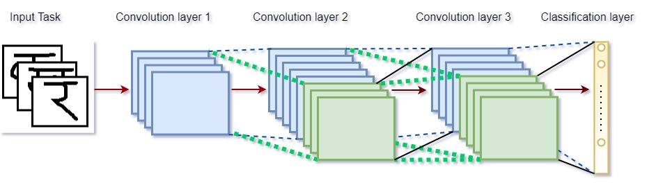
Figure 1: This diagram shows the proposed MAC model $M^{\prime}$. The neural network inputs a batch of task and modifies the weights of the networks in each iterations. Each convolution layer has blue and green filters. The blue filters are the base modules and green filters are the newly added units(ACUs). Blue dashed lines are the old connection of the base model M, Whereas green dotted connections are the new links with the old and new nodes. Solid black lines are zero weight connections.

The new model $M^{\prime}$ (Figure.1) is formed by adding additional connection units in the body of the base model $M$. An illustration of the proposed network model $M^{\prime}$ for meta-testing is shown in fig.1. For each ${}^{\prime}l^{\prime}$ layer {${1,2,3,...,L}$} of the network $f$ takes input as an image of the task and outputs a class label for the corresponding task image. The ACUs are added on $\{L-1\}$ layers of the network. Let $\theta^{*}=(\theta_{1}^{*},\theta_{2}^{*},...,\theta_{L}^{*})$ be the meta-trained parameters for the each layer of the network. We initialise layer weights of the MAC model $M^{\prime}$ with $\theta^{*}$.
For $L-1$ layers: The weight matrix ${W_{l}}$ for the body of the network {${l=1,2,...,L-1}$} is initialised as:

$$W_{l}=\begin{pmatrix}\theta^{*}_{l}&0\\ W_{l1}&W_{l2}\end{pmatrix},\\ b^{l}=\begin{pmatrix}b^{*}_{l}\\ b_{l}\end{pmatrix}$$ (5)

where,${W_{l1}}$ are weights w.r.t the connections between ACU and base layer. ${W_{l2}}$ are new weights w.r.t the connections between ACUs. Both ${W_{l1}}$ and ${W_{l2}}$ are randomly initialized weights. The zero weights are initialised for the connection between new to old nodes of the network.
Similarly, $b_{l}$ is randomly initialised bias for ACUs and $b^{*}_{l}$ is the meta-trained bias obtained during meta-training.

For $L^{th}$ layer: The weights and bias matrices for classifier layer of model $M^{\prime}$ will be initialised as:

$$W_{L}=\begin{pmatrix}\theta^{*}_{L}&0\end{pmatrix},b_{L}=\begin{pmatrix}b^{*}_{L}\end{pmatrix}$$ (6)

where, $\theta^{*}_{L}$ is the meta-trained parameters of the classifier layer and zero weights are the connection weights from newly added ACUs to classifier layer nodes.

5.2 MAC Training

Meta-training is performed on a batch of $m$ tasks drawn from the training data distribution $p(D^{tr})$. $\theta$ be the initial parameters for [L-1] layers, and $\mu$ be the initial classifier layer parameter of the base model $M$. Initially, both the parameters are randomly initialized. The process of Meta-training for MAC and ANILfinn2017model algorithm is same. For each batch of task $T_{i}$, we perform two updates:
1) In inner loop gradient updates, we only update the classifier layer weights $\mu$ of the proposed model $M$.
2) During the outer loop update, we calculate and update the gradients of the model $M$ after each inner loop updation.

Finally, we get our meta initialized parameters $\theta^{*}$ for [L-1] layers and $\mu^{*}$ for the classifier layer. Note that $\mu$ is updated in both the inner and outer loop, but $\theta$ is updated only during the outer loop.

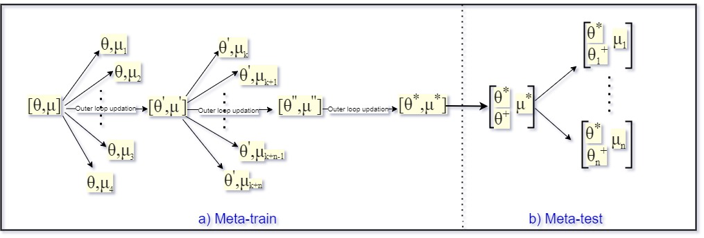
Figure 2: Part (a) illustrates the meta-training phase of our proposed MAC algorithm where it finds meta-initialization parameters $\theta^{*}$ and $\mu^{*}$ after the final outer loop updation for the model $M^{\prime}$ so that new tasks are learnt rapidly with additional feature learning and recombination, part (b) Represents model $M^{\prime}$ with additional links to the [L-1] layers shown as ${\theta^{+}}$ and the classifier layer weights as $\mu^{*}$ obtained during meta-training to perform task adaptation.

5.3 MAC Testing

Fig. 2(b). illustrates the meta-testing phase on model $M^{\prime}$ for the data whose distribution is not similar to the training data distribution. To achieve this, we update our model $M$ by adding extra links in the [L-1] layers. These links are ACUs and are represented as $\theta^{+}$ in the diagram. The model is initialized with meta-trained parameters $\theta^{*}$ and $\mu^{*}$. Whereas $\theta^{+}$ are the randomly initialized parameters of newly added ACUs. These additional links in the network are designed to capture new atomic features of the perturbed tasks, which then recombine with the meta-trained parameters and perform few-shot-learning. During meta-testing, each task updates the ACU parameter($\theta+$) and the classifier layer($\mu^{*}$) parameters to perform meta-adaptation on the new unseen tasks.

For a clearer view, we will see how the parameters are updated during forward and backward pass.
a) Forward pass: Refer to Fig. 1 and 2, the model $M^{\prime}$ has two coloured filters in the last two hidden layers(the number of hidden layers may vary). Blue colored filters are meta-trained parameters($\theta^{*},\mu$) of model M and green filters are the parameters of ACU($\theta^{+}$). During forward pass, the image of task T' is passed through each layer of model $M^{\prime}$. An extended feature map is obtained by the newly added ACUs and propagated to the next layer during the forward pass.
b) Backward pass: In backward pass, loss and gradients are backpropagated through a subset of connections only (green dots) in fig. 1. In contrast, some gradients are intentionally made zero (solid black lines) initially. Later, during the meta-adaptation phase, these zeroed-out weights will get updated. In effect, this will force the model to learn the new atomic features and update only the parameters of ACUs and the classifier layer.

The ACUs learn new features and recombine them with learned features obtained during the meta-training phase for every task. Algorithm 1 explains the proposed MAC algorithm during meta-testing.

Algorithm 1 Algorithm for meta-testing

Initialize:'$\alpha$' learning rate, 'n' step size, size of ACU

1:Initialize $\theta^{*}$ and $\mu^{*}$ from meta-traininig.

2:Sample a batch of tasks ${T^{\prime}}_{i}$ from ${D^{ts}}$

3:for all i  do

4:     Sample $K$ datapoints $\{{{x^{\prime}}_{j},{y^{\prime}}_{j}}\}$ from $\mathcal{T^{\prime}}_{i}$(N-way K-shot).

5:     Initialize additional connection units as ${\theta^{+}}\sim(\mathcal{N}(0,1))$ : and Let, $\Theta\rightarrow[{\theta^{*}},{\theta^{+}},{\mu^{*}}],$

6:     Evaluate $\nabla_{[\theta^{+},\mu^{*}]}{\mathcal{L}_{\mathcal{T}_{i}}}$ using stochastic gradient descent for n-steps.

7:     Update the network parameters: $\Theta^{\prime}=\Theta-\alpha{\nabla_{[{\Theta^{+}},{\mu^{*}}]}}\mathcal{L}_{\mathcal{T}_{i}}(f_{\Theta})$

8:     Compute accuracy: ${a_{i}}\leftarrow accuracy({{T^{\prime}}_{i}},\Theta^{\prime})$ Total accuracy = ${\frac{1}{\mathcal{T}}}{\sum_{i=1}^{i}a_{i}}$

9:end forreturn Total accuracy

6 Implementation Details and Results

6.1 System Configuration

We have performed all our experiments on 2 GPU server with the following configurations:
2x Tesla-V100 : 16GB
RAM : 32 GB
CUDA cores = 10,240
CUDA version: V9.2.148 System type : 64-bit Operating System,x64-based processor.

6.2 Dataset

We have used two standard benchmark datasets often used for a few shot learning paradigms.

6.2.1 Omniglot

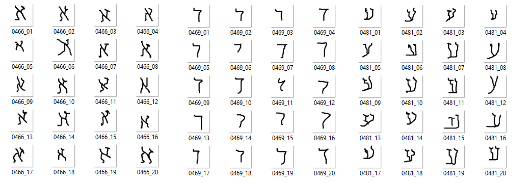
Figure 3: Three sets of different character depicting three classes from Omniglot dataset. ${char1}$, $char4$ and $char16$ in Hebrew. Each character is written by $20$ different person.

To evaluate our proposed model, We perform our experiments on the Omniglot dataset lake2011one for classification. This dataset contains 50 different alphabets divided into 1623 handwritten characters known as classes. Each class has 20 black and white images of size 28X28 drawn by 20 different persons. The images are labelled with the name of the corresponding character and a suffix. For, e.g. the Alphabet of the Sanskrit language in the dataset has 42 characters, and there are 20 images of each character with labels. In our classification task, each character is considered a separate class irrespective of language. These classes are split into training and test sets: 1200 classes for training and 423 class for testing. All the character images are first augmented by performing rotations to create more data samples and reduce overfitting. Figure 1 illustrates some Hebrew language characters.

6.2.2 MiniImagenet

Ravi and Larochelle proposed the MiniImagenet dataset in the year 2016vinyals2016matching . The dataset consists of 64 training classes, 24 test classes and 12 validation classes. We consider four task settings, i.e., 5-way 1-shot, 5-way 5-shot, 10-way 5-shot and 10-way 1-shot on this dataset. Therefore, we have meta-train and meta-test tasks to classify among 20 randomly chosen different classes, given only a few labelled samples, i.e., 5 and 1 instance of each class. The experiments are done for 5-way 1-shot and 5-way 5-shot task settings.

6.3 Implementation Details

6.3.1 Data from non-identical distribution

The main idea is to perform meta-adaptation during meta-testing on the different data distributions to show that the new atomic features are learned using the newly added ACUs. Whereas, in traditional few shot learinngfinn2017model , task distribution for meta-training and meta-testing are the same. The meta-test tasks are never seen beforehand, and meta-learning assumes it to be from the same distribution as the meta-training task distribution, which is more likely to perform task-adaptation on learned parameters. Past researches performed cross-domain few-shot learning oh2020boil miranda2021does and used different datasets to perform meta-learning. Unlike others, we created meta-testing data using the actual datasets(omniglot, miniimagenet) and converted it to different distributions using gaussian blur. In terms of method, our work is more similar to ANIL raghu2019rapid , and this is because we clubbed our idea of additional connection units with existing almost no inner loop known as MAC to perform meta-learning for heterogeneous data.

6.3.2 Few-Shot classification

We used PyTorch and Torchmeta deleu2019torchmeta ANIL implementation. For a few-shot classification, we used the same model architecture as used in the original MAML implementation finn2017model . To perform N-way k-shot classification, We trained our model using an omniglot dataset for 60000 iterations with a batch size of 32 tasks, three gradient steps, a learning rate of 0.4 and the model is evaluated on a batch size of 32 with step size 0.4. For the Miniimagenet dataset, the model was trained for 60000 iterations, using five gradient steps, batch size of 4 and learning rate of 0.01 and is evaluated using two different learning rates: 0.1 for hidden layers and 0.02 for the classifier layer with ten gradient steps and batch size of 4.

We tested our proposed MAC model on 100 batches of unseen tasks using 10 inner stochastic gradient descent steps. We performed several experiments to commit the final observation. We evaluated our model 3 times with different random seeds and calculated the mean of all the results to show the absolute average accuracy. Further, we bound the number of ACUs added should not be more than 50 units. Since we aim to capture only the atomic features. Therefore, the proposed model enhances the few-shot learning ability that can reuse and recombine the features to adapt to a new task efficiently without complicating the network architecture.

6.4 Results and Discussion

Few-shot-classification for the MAC model needs some clear experimental results for deciding:
Why we need ACUs?
How many ACUs are required to learn important atomic features of the new dataset?
Where should we add ACUs in our proposed model?
What happens if we increase the depth of our model?
The experimental results and explanations are given below:

6.4.1 Need for ACUs

The main idea behind adding the ACUs is to increase the width of the network. In the meta-learning scenario, it is imperative to learn new atomic features when the meta-testing tasks are drawn from a non-identical distribution. This would require unfreezing parameters of the entire network to enable learning new atomic features in the lower layers, followed by their combination in the higher layers. However, this would lead to unlearning meta-train parameters, effectively stopping the making of the meta-learning process, especially when a non-negligible number of new atomic features needed to be learnt. We can increase the width of the network by adding ACUs to learn new features and reuse the existing features by retaining the learnt parameters to meet the objectives of learning, reuse and recombination. Fig.4.(a) shows the equal learning accuracies for both MAC and ANIL algorithms. This means ACUs in the MAC method do not capture any new features as new atomic features are absent in the same task distribution settings. Whereas fig.4.(b) shows high accuracy for the MAC method, proving that ACUs in the MAC method are responsible for capturing and recombining new extra features during the task adaptation phase.

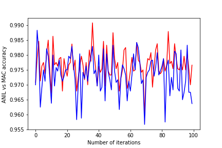
(a) ANIL vs MAC meta-test accuracy on same data distribution(without perturbation).Blue line shows the MAC accuracy and red line shows the ANIL accuracy.

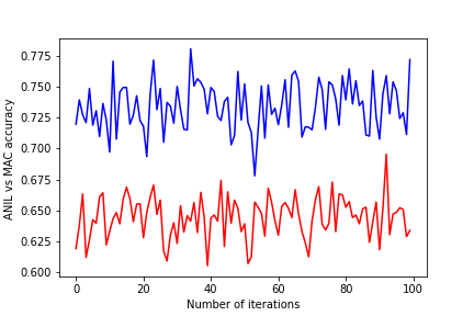
(b) ANIL vs MAC meta-test accuracy on perturbed distribution. Blue line shows the MAC accuracy and red line shows the ANIL accuracy.

Figure 4: 5-way 5-shot test accuracy graph.

6.4.2 Number of ACUs

How many node connections should be added to each layer? The size of the ACUs is decided by iterative testing performed for different combinations of nodes for the entire network. We limit our maximum number of nodes to be 50 only. Since we need to extract and recombine the new atomic features of the unseen tasks, we require small connection units. However, The size of ACUs is not fixed for all the target task settings, i.e., the size differs for every few-shot task setup. For instance, the optimal number of ACUs added in the model for a 5-way 5-shot task setting is [50, 30, 20, 5], but for a 10-way 5-shot task, it is [50,35,20,10]. It is evident from the sizes of each layer ACU that the new features require initial layer feature extraction with larger units and feature recombination at the rearmost layers with smaller units.
After examining every combination of nodes, we found one combination to be optimal for all tasks, i.e., For omniglot: $MAC_{opt}$ = [45,35,20,10]. Table V.a shows the experimental results for fixed number of ACUs ($MAC_{opt}$) vs ($MAC_{best}$). For miniimagenet: $MAC_{opt}$ = [50,40,25,20]. Table V.b shows the experimental results for fixed number of ACUs ($MAC_{opt}$) vs ($MAC_{best}$).

6.4.3 Position of ACUs

Our base model $M$ is similar to ANILraghu2019rapid model. The model has 4 modules; each module consists of a 3 x 3 convolution layer, 64 filters with stride 2, followed by a batch normalization layer and reLU at last. We can add a maximum of 4 ACU units, i.e., one ACU per module, in our base model $M$. To decide where should we add the ACUs, we performed experiments by adding units to each convolution layer and examined the results. Let model $M$ having $L$ layers, and then we add units to at most $L-1$ hidden layers as follows:

a) At the beginning of the model: For our proposed method MAC, we add connections in the initial layers $\{ACU_{1},ACU_{2},0,0\}$ of the model $M$. We examined the number of optimal ACUs to be added in the initial layers of the model (refer to Table I(a) and I(b) ).

(a) Table I.a: Omniglot+Gaussian blurr Dataset

Methods	5-w 1-s	5-w 5-s	10-w 1-s	10-w 5-s
ANIL	41.65	64.43	30.87	49.88
MAC	43.41	73.87	32.45	56.35
Units	[25,45,0,0]	[25,50,0,0]	[25,45,0,0]	[25,50,0,0]

(b) Table I.b: Miniimagenet+Gaussian blurr Dataset

Methods	5-w 1-s	5-w 5-s
ANIL	26.43	35.88
MAC	26.41	36.00
Units	[20,40,0,0]	[45,5,0,0]

b) At the end of model $M$: we added a few ACUs on the last few layers except the classifier layer $\{0,0,ACU_{1},ACU_{2}\}$ of the model $M$. We further calculated the optimal number of connections to be added in a few last layers of the model ( refer to tables II(a) and II(b)).

(c) Table II.a: Omniglot+Gaussian blurr Dataset

Methods	5-w 1-s	5-w 5-s	10-w 1-s	10-w 5-s
ANIL	41.65	64.43	30.87	49.88
MAC	43.62	74.10	31.52	56.60
Units	[0,0,50,20]	[0,0,45,5]	[0,0,50,20]	[0,0,50,5]

(d) Table II.b: Miniimagenet+Gaussian blurr Dataset

Methods	5-w 1-s	5-w 5-s
ANIL	26.43	35.88
MAC	26.40	35.50
Units	[0,0,40,15]	[0,0,45,5]

c) Throughout the model $M$: We added 4 ACUs in each convolution layer except the input and classifier layer $\{ACU_{1},ACU_{2},ACU_{3},ACU_{4}\}$ of the model $M$ ( refer to table III(a) and III(b)).

(e) Table III.a: Omniglot+Gaussian blurr Dataset

Methods	5-w 1-s	5-w 5-s	10-w 1-s	10-w 5-s
ANIL	41.65	64.43	30.87	49.88
MAC	44.12	74.52	33..42	57.18
Units	[50,40,20,10]	[50,30,20,5]	[50,25,20,10]	[50,35,20,10]

(f) Table III.b: Miniimagenet+Gaussian blurr Dataset

Methods	5-w 1-s	5-w 5-s
ANIL	26.43	35.88
MAC	27.17	38.51
Units	[50,35,15,5]	[50,35,40,10]

6.4.4 Adding layers to the base model

In this section, we will find out an answer to a question, i.e., Will the performance of the proposed method increases if we add some layers to the model?
A promising workarnold2021maml done in the past unveils some interesting unknown properties of the MAML algorithm. Their study found that the MAMLfinn2017model is well suited to the depth of the model architecture. Inspired by this, we evaluated our proposed method for the deeper model. To make our model "deep", we add a few Convolution layers to the rearmost of the proposed MAC model $M^{\prime}$. Further, to evaluate the meta-adaptation performance of this approach, we used two different models. First, the MAC model $M^{\prime}$ and second, the deep model ${M^{\prime}}_{deep}$. The deep model adds two Convolution layers in the base model $M$. We performed few-shot classification experiments on both the models ($M^{\prime}$ and ${M^{\prime}}_{deep}$). Model ${M^{\prime}}_{deep}$ consists of 6 modules: 4 modules with 3X3 convolutions and 64 filters with stride(2), followed by Batchnorm and a ReLU activation function and 2 additional modules of a Convolution layer, each followed by a Batchnorm and a ReLU activation functions. The model $M_{deep}$ is trained and tested for two datasets (Omniglot and Miniimagenet) on similar hyperparameters (Section 6.3.2).

(g) Table IV.a: Omniglot+Gaussian blurr Dataset

Method	5-way 1-shot	5-way 5-shot
ANIL	41.65	64.43
MAC	44.12	74.52
$MAC_{deep}$	43.59	75.77

(h) Table IV.b: Miniimagenet+Gaussian blurr Dataset

Methods	5-w 1-s	5-w 5-s
ANIL	26.43	35.88
MAC	27.02	36.12
$MAC_{deep}$	23.59	37.31

(i) Table V.a: Omniglot+Gaussian blurr Dataset

Method	5-way 1-shot	5-way 5-shot	10-way 1-shot	10-way 5-shot
ANIL	41.65	64.43	30.87	49.88
$MAC_{best}$	44.12	74.52	33.42	57.18
$MAC_{opt}$	43.81	74.45	33.10	56.93

(j) Table V.b: Miniimagenet+Gaussian blurr Dataset

Method	5-way 1-shot	5-way 5-shot
ANIL	25.87	34.82
$MAC_{best}$	27.02	36.12
$MAC_{opt}$	26.43	35.88

6.4.5 Effect of shallow vs deep meta-learning model

We observed increased accuracy that is directly due to enhanced meta-learning when depth is increased. The results(table IV.a and IV.b) shows the change in performance metric with the shallow MAC model($M^{\prime}$) and the deep model $MAC_{deep}$.

Therefore, it is evident from the results that depth facilitates few-shot learning when added to a base model. After repetitive testing, we made an observation that the results were best for a 5-way 5-shot task setting for both omniglot and miniimagenet datasets.

7 Conclusion

In this paper, we increased the width of the network by adding computational units to make a provision for learning new features present in the meta-test tasks while keeping the parameters of the base network unchanged. This allowed meta-learning when new feature learning during meta-testing is required. The method enabled few shot classifications on perturbed tasks with higher accuracy than methods that preclude new feature learning. Results show that both feature recombination and feature learning are necessary for meta-testing in tasks that are independent but non-identical from the meta-training task distribution. We also discovered that adding new connections should be done in a restricted manner to discourage increased complexity and computational overhead in the model. Also, a gradual decrease in the number of connections moving from the initial to the final layer proved beneficial to the model's performance. The follow-up analysis on the effect of depth showed that it indeed increases the abstraction level by 10-12 percentage. We can conclude by stating two important findings of the work. One, only feature reuse is sufficient for meta-learning and two, few-shot-learning performance is enhanced by increasing the width and depth of the base model during meta-testing.

Data Availability Data can be available on demand.

Funding No funds or grants were received from any organization.

Declaration

Conflict of Interest The authors have no conflict of interest to declare to the best of their knowledge.

References

- \bibcommenthead
- (1) Koch, G., Zemel, R., Salakhutdinov, R., et al.: Siamese neural networks for one-shot image recognition. In: ICML Deep Learning Workshop, vol. 2, p. 0 (2015). Lille
- (2) Vinyals, O., Blundell, C., Lillicrap, T., Wierstra, D., et al.: Matching networks for one shot learning. Advances in neural information processing systems 29 (2016)
- (3) Snell, J., Swersky, K., Zemel, R.: Prototypical networks for few-shot learning. Advances in neural information processing systems 30 (2017)
- (4) Finn, C., Abbeel, P., Levine, S.: Model-agnostic meta-learning for fast adaptation of deep networks. In: International Conference on Machine Learning, pp. 1126–1135 (2017). PMLR
- (5) Santoro, A., Bartunov, S., Botvinick, M., Wierstra, D., Lillicrap, T.: Meta-learning with memory-augmented neural networks. In: International Conference on Machine Learning, pp. 1842–1850 (2016). PMLR
- (6) Ravi, S., Larochelle, H.: Optimization as a model for few-shot learning (2016)
- (7) Nichol, A., Achiam, J., Schulman, J.: On first-order meta-learning algorithms. arXiv preprint arXiv:1803.02999 (2018)
- (8) Raghu, A., Raghu, M., Bengio, S., Vinyals, O.: Rapid learning or feature reuse? towards understanding the effectiveness of maml. arXiv preprint arXiv:1909.09157 (2019)
- (9) Bengio, S., Bengio, Y., Cloutier, J., Gecsei, J.: On the optimization of a synaptic learning rule. In: Preprints Conf. Optimality in Artificial and Biological Neural Networks, vol. 2 (1995)
- (10) Hochreiter, S., Younger, A.S., Conwell, P.R.: Learning to learn using gradient descent. In: International Conference on Artificial Neural Networks, pp. 87–94 (2001). Springer
- (11) Munkhdalai, T., Yu, H.: Meta networks. In: International Conference on Machine Learning, pp. 2554–2563 (2017). PMLR
- (12) Sung, F., Yang, Y., Zhang, L., Xiang, T., Torr, P.H., Hospedales, T.M.: Learning to compare: Relation network for few-shot learning. In: Proceedings of the IEEE Conference on Computer Vision and Pattern Recognition, pp. 1199–1208 (2018)
- (13) Li, Z., Zhou, F., Chen, F., Li, H.: Meta-sgd: Learning to learn quickly for few-shot learning. arXiv preprint arXiv:1707.09835 (2017)
- (14) Triantafillou, E., Zhu, T., Dumoulin, V., Lamblin, P., Evci, U., Xu, K., Goroshin, R., Gelada, C., Swersky, K., Manzagol, P.-A., et al.: Meta-dataset: A dataset of datasets for learning to learn from few examples. arXiv preprint arXiv:1903.03096 (2019)
- (15) Zhang, R., Che, T., Ghahramani, Z., Bengio, Y., Song, Y.: Metagan: An adversarial approach to few-shot learning. Advances in neural information processing systems 31 (2018)
- (16) Oreshkin, B., Rodríguez López, P., Lacoste, A.: Tadam: Task dependent adaptive metric for improved few-shot learning. Advances in neural information processing systems 31 (2018)
- (17) Jamal, M.A., Qi, G.-J.: Task agnostic meta-learning for few-shot learning. In: Proceedings of the IEEE/CVF Conference on Computer Vision and Pattern Recognition, pp. 11719–11727 (2019)
- (18) Antoniou, A., Edwards, H., Storkey, A.: How to train your maml. arXiv preprint arXiv:1810.09502 (2018)
- (19) Yao, H., Wei, Y., Huang, J., Li, Z.: Hierarchically structured meta-learning. In: International Conference on Machine Learning, pp. 7045–7054 (2019). PMLR
- (20) Zintgraf, L., Shiarli, K., Kurin, V., Hofmann, K., Whiteson, S.: Fast context adaptation via meta-learning. In: International Conference on Machine Learning, pp. 7693–7702 (2019). PMLR
- (21) Sun, Q., Liu, Y., Chua, T.-S., Schiele, B.: Meta-transfer learning for few-shot learning. In: Proceedings of the IEEE/CVF Conference on Computer Vision and Pattern Recognition, pp. 403–412 (2019)
- (22) Rusu, A.A., Rao, D., Sygnowski, J., Vinyals, O., Pascanu, R., Osindero, S., Hadsell, R.: Meta-learning with latent embedding optimization. arXiv preprint arXiv:1807.05960 (2018)
- (23) Chen, W.-Y., Liu, Y.-C., Kira, Z., Wang, Y.-C.F., Huang, J.-B.: A closer look at few-shot classification. arXiv preprint arXiv:1904.04232 (2019)
- (24) Tian, Y., Wang, Y., Krishnan, D., Tenenbaum, J.B., Isola, P.: Rethinking few-shot image classification: a good embedding is all you need? In: European Conference on Computer Vision, pp. 266–282 (2020). Springer
- (25) Fan, F.-L., Lai, R., Wang, G.: Quasi-equivalence of width and depth of neural networks. arXiv preprint arXiv:2002.02515 (2020)
- (26) Nguyen, T., Raghu, M., Kornblith, S.: Do wide and deep networks learn the same things? uncovering how neural network representations vary with width and depth. arXiv preprint arXiv:2010.15327 (2020)
- (27) Nguyen, Q., Hein, M.: The loss surface of deep and wide neural networks. In: International Conference on Machine Learning, pp. 2603–2612 (2017). PMLR
- (28) Lake, B., Salakhutdinov, R., Gross, J., Tenenbaum, J.: One shot learning of simple visual concepts. In: Proceedings of the Annual Meeting of the Cognitive Science Society, vol. 33 (2011)
- (29) Oh, J., Yoo, H., Kim, C., Yun, S.-Y.: Boil: Towards representation change for few-shot learning. arXiv preprint arXiv:2008.08882 (2020)
- (30) Miranda, B., Wang, Y.-X., Koyejo, S.: Does maml only work via feature re-use? a data centric perspective. arXiv preprint arXiv:2112.13137 (2021)
- (31) Deleu, T., Würfl, T., Samiei, M., Cohen, J.P., Bengio, Y.: Torchmeta: A Meta-Learning library for PyTorch. Available at: https://github.com/tristandeleu/pytorch-meta (2019). https://arxiv.org/abs/1909.06576
- (32) Arnold, S., Iqbal, S., Sha, F.: When maml can adapt fast and how to assist when it cannot. In: International Conference on Artificial Intelligence and Statistics, pp. 244–252 (2021). PMLR