Mirror Prox Algorithm for Large-Scale Cell-Free Massive MIMO Uplink Power Control

Abstract

We consider the problem of max-min fairness for uplink cell-free massive multiple-input multiple-output (MIMO) subject to per-user power constraints. The standard framework for solving the considered problem is to separately solve two subproblems: the receiver filter coefficient design and the power control problem. While the former has a closed-form solution, the latter has been solved using either second-order methods of high computational complexity or a first-order method that provides an approximate solution. To deal with these drawbacks of the existing methods, we propose a mirror prox based method for the power control problem by equivalently reformulating it as a convex-concave problem and applying the mirror prox algorithm to find a saddle point. The simulation results establish the optimality of the proposed solution and demonstrate that it is more efficient than the known methods. We also conclude that for large-scale cell-free massive MIMO, joint optimization of linear receive combining and power control provides significantly better user fairness than the power control only scheme in which receiver coefficients are fixed to unity.

I Introduction

The recently evolved form of the massive multiple-input multiple-output (MIMO) for the beyond fifth generation (5G) networks is cell-free massive MIMO [1], in which one or several central processing units (CPUs) control a large number of low-cost and low-power access points to serve a large number of users. The APs and users are distributed in a large coverage area. Owing to the high array gain, multiplexing gain, and macro-diversity gain, cell-free massive MIMO offers many advantages such as high energy efficiency, uniform quality of service, and flexible and cost-effective deployment [2].

To achieve the above benefits, suitable power allocation algorithms need to be employed to control the near/far effect. Since the numbers of APs and users are large, the resulting power control problems consist of many variables. Thus, simple and low-complexity solutions to power control optimization problems for cell-free massive MIMO are of particular interest. In [1], the problem of maximization of the minimum uplink rate (a.k.a. max-min fairness) for single-antenna APs and single-antenna users was solved using a bisection algorithm in combination with linear programming (LP), where maximum-ratio combining (MRC) was considered at each AP for signal detection. In [3], Bashar et al. solved this max-min fairness problem by alternatively solving two subproblems: (i) the receiver coefficient design which is in fact a generalized eigenvalue problem (EVP), and (ii) the power control problem which was solved using geometric programming (GP). A similar alternating optimization (AO)-based scheme was used in [4] to solve a mixed quality of service (QoS) problem including the max-min fairness for a set of users and a fixed QoS for the remaining users. Again, the power control subproblem was solved using GP. In [5], Mai et al. employed the zero-forcing (ZF) technique to detect symbols from multi-antenna users where the power control problem was solved using the bisection algorithm. A common feature of all aforementioned studies is the use of LP or (more complex) GP by means of off-the-shelf convex solvers, and thus are suitable for small-scale scenarios. In particular, a low complexity first-order accelerated projected gradient (APG) algorithm was applied to the max-min fairness problem following Nesterov’s smoothing technique [6] in both downlink [7, 8] and uplink [9] channels. However, this method can only produce an approximate solution whose accuracy is inversely proportional to the number of users, and hence, is not suitable for very large numbers of users. This clearly calls for novel solutions to the power control problem, which are more computationally efficient than LP or GP methods and more accurate than the APG method.

In this paper, we consider the max-min fairness problem subject to the power constraint at each user. We utilize the MRC technique to detect users’ signals using the channel estimates. Similar to the known approaches, we also split the considered problem into two subproblems which are alternately solved. In particular, for the power control subproblem, we propose a mirror prox (MP)-based algorithm. To achieve this, we first reformulate the nonconvex power control problem into an equivalent convex-concave program and then propose an MP method [10] to find a saddle point. The proposed method only requires the first order information of the objective, and thus, is shown to be much faster than the LP-based and GP-based methods. Moreover, it outperforms other existing first-order methods in terms of achievable rate performance.

Notations: Bold lower and upper case letters represent vectors and matrices. $\mathcal{CN}(\boldsymbol{0},\mathbf{K})$ denotes the multivariate circularly symmetric complex Gaussian random distribution with zero mean and co-variance matrix $\mathbf{K}$. $\mathbf{X}^{\mbox{\scriptsize T}}$ and $\mathbf{X}^{\mbox{\scriptsize H}}$ stand for the transpose and Hermitian of $\mathbf{X}$, respectively. Notation $\mathbf{e}_{i}$ denotes the $i$-th column of the identity matrix. $\nabla f(\mathbf{x})$ represents the gradient of $f(\mathbf{x})$. $\left\|\cdot\right\|$ denotes the Euclidean or $\ell_{2}$-norm and $|\cdot|$ is the absolute value of the argument. $\mathcal{P}_{\mathcal{C}}(\mathbf{x})$ denotes the projection of $\mathbf{x}$ onto the convex set $\mathcal{C}$, i.e. $\mathcal{P}_{\mathcal{C}}(\mathbf{x})=\underset{\mathbf{z}\in\mathcal{C}}{\arg\min}\bigl{\|}\mathbf{x}-\mathbf{z}\bigr{\|}$.

II System Model and Problem Formulation

Consider a cell-free massive MIMO uplink scenario where $L$ single-antenna users are served by $M$ APs with $K$ antennas per AP. All APs and users are randomly distributed in a coverage area. The APs are connected to a CPU via high-capacity dedicated links. We denote by $\zeta_{ml}$ the large-scale fading coefficient between the $l$-th user and the $m$-th AP, and $\tilde{\mathbf{h}}_{ml}\sim\mathcal{CN}(\boldsymbol{0},\textbf{I}_{K})$ is the vector of the small-scale fading coefficient for all antennas at the $m$-th AP. The channel vector between the $l$-th user and the $m$-th AP is modeled as

$$\mathbf{h}_{ml}=\zeta_{ml}^{1/2}\tilde{\mathbf{h}}_{ml}.$$ (1)

The length (in symbols) of the uplink training is denoted by $\tau_{p}$. Let $\eta_{p}$ be the transmit power of each pilot symbol and $\boldsymbol{\phi}_{l}$ be the pilot sequence of unit norm transmitted from user $l$ to the APs. Let $\hat{\mathbf{h}}_{ml}$ be the minimum mean square error (MMSE) channel estimate of $\mathbf{h}_{ml}$. Then $\hat{\mathbf{h}}_{ml}\sim\mathcal{CN}(\boldsymbol{0},g_{ml}\textbf{I}_{K})$, where [1]

$$g_{ml}\triangleq\frac{\eta_{p}\tau_{p}\zeta_{ml}^{2}}{\eta_{p}\tau_{p}\sum_{i=1}^{L}\zeta_{mi}\left|\boldsymbol{\phi}_{i}^{\mbox{\scriptsize H}}\boldsymbol{\phi}_{l}\right|^{2}+1}.$$ (2)

To formulate the problem of interest, we define $\mathbf{p}=[p_{1},\ldots,p_{L}]$ as the vector of power control coefficients, $\mathbf{q}=[\mathbf{q}_{1};\mathbf{q}_{2};\ldots;\mathbf{q}_{L}]$ as the receiver coefficient where $\mathbf{q}_{l}=[q_{1l};q_{2l};\ldots;q_{Ml}]$ associates with the $l$-th user, and $\bar{p}$ as the maximum transmit power at each individual user. With this setup, an achievable signal-to-interference plus noise ratio (SINR) is given by [1]

$$\gamma_{l}(\mathbf{p},\mathbf{q})=\frac{\mathbf{q}_{l}^{\mbox{\scriptsize H}}\bigl{(}\mathbf{g}_{ll}\mathbf{g}_{ll}^{\mbox{\scriptsize H}}p_{l}\bigr{)}\mathbf{q}_{l}}{\mathbf{q}_{l}^{\mbox{\scriptsize H}}\bigl{(}\sum_{i\neq l}^{L}\mathbf{g}_{li}\mathbf{g}_{li}^{\mbox{\scriptsize H}}p_{i}+\frac{1}{K}\sum_{i=1}^{L}\bar{\mathbf{G}}_{li}p_{i}+\frac{1}{K}\tilde{\mathbf{G}}_{l}\bigr{)}\mathbf{q}_{l}}.$$ (3)

In (3), $\bar{\mathbf{G}}_{li}\in\mathbb{R}_{+}^{M\times M}$ and $\tilde{\mathbf{G}}_{l}\in\mathbb{R}_{+}^{M\times M}$ are diagonal matrices with $[\bar{\mathbf{G}}_{li}]_{m,m}=g_{ml}\zeta_{mi}$ and $[\tilde{\mathbf{G}}_{l}]_{m,m}=g_{ml}$, respectively, and

$$\mathbf{g}_{li}\triangleq\left|\boldsymbol{\phi}_{l}^{\mbox{\scriptsize H}}\boldsymbol{\phi}_{i}\right|\left[g_{1l}\frac{\zeta_{1i}}{\zeta_{1l}};g_{2l}\frac{\zeta_{2i}}{\zeta_{2l}};\ldots;g_{Ml}\frac{\zeta_{Mi}}{\zeta_{Ml}}\right].$$ (4)

Note that the achievable rate of the $l$-th user is given by

$$\mathcal{R}_{l}(\mathbf{p},\mathbf{q})=\log_{2}\left(1+\gamma_{l}(\mathbf{p},\mathbf{q})\right).$$ (5)

Similar to [3], we consider the problem of maximization of the minimum rate, which is mathematically stated as

$$\begin{array}[]{ll}\underset{\mathbf{q},\mathbf{p}}{\operatorname{maximize}}&\quad\underset{1\leq l\leq L}{\min}\gamma_{l}(\mathbf{p},\mathbf{q})\\ \operatorname{subject\,to}&\quad\left\|\mathbf{q}_{l}\right\|=1,\,l=1,\ldots,L,\\ &\quad 0\leq\mathbf{p}\leq\bar{p}.\end{array} \mathcal{P}_{1}$$ ()

First, we note that ($\mathcal{P}_{1}$) is nonconvex, and thus, finding a globally optimal solution is difficult and not practically useful. The standard framework for solving ($\mathcal{P}_{1}$) which is adopted in previous studies such as [1, 3, 4] is based on AO. In this way, two subproblems arise: the receiver coefficient design and the power control problem. Specifically, the receiver coefficient design is obtained by fixing the power allocation $\mathbf{p}$, which admits a closed-form solution given by [3, 4]

$$\mathbf{q}_{l}^{*}=\frac{\sqrt{p_{l}}\mathbf{W}_{l}^{-1}\mathbf{g}_{ll}}{\bigl{\|}\sqrt{p_{l}}\mathbf{W}_{l}^{-1}\mathbf{g}_{ll}\bigr{\|}},l=1,2,\ldots,L,$$ (6)

where $\mathbf{W}_{l}=\sum_{i\neq l}^{L}\mathbf{g}_{li}\mathbf{g}_{li}^{\mbox{\scriptsize H}}p_{i}+\frac{1}{K}\sum_{i=1}^{L}\bar{\mathbf{G}}_{li}p_{i}+\frac{1}{K}\tilde{\mathbf{G}}_{l}$. After updating the receiver coefficients for all users, we need to find the power coefficients, leading to the following power control problem:

$$\boxed{\underset{0\leq\mathbf{p}\leq\bar{p}}{\operatorname{maximize}}\quad\underset{1\leq l\leq L}{\min}\gamma_{l}(\mathbf{p})} \mathcal{P}_{2}$$ ()

To solve ($\mathcal{P}_{2}$), existing methods [1, 3, 4] involve second order methods, i.e., GP or LP, which require very high complexity, and thus, is not suitable for large-scale cell-free massive MIMO. To overcome the complexity issue, a first-order algorithm was introduced in [9] but it cannot yield a solution of high accuracy for a large number of users. In the next section, we propose a more efficient method for solving ($\mathcal{P}_{2}$) based on the MP framework.

III Proposed Solution for Power Control Problem

III-A Equivalent Convex-Concave Reformulation of ($\mathcal{P}_{2}$)

The proposed method is developed based on an equivalent convex-concave reformulation of ($\mathcal{P}_{2}$). To this end, it is easy to see that we can equivalently rewrite ($\mathcal{P}_{2}$) as

$$\underset{\mathbf{p}}{\operatorname{minimize}}\ \underset{1\leq l\leq L}{\max}\gamma_{l}^{-1}(\mathbf{p}),$$ (7)

where

$$\gamma_{l}^{-1}(\mathbf{p}) =p_{l}^{-1}\Bigl{(}\sum\nolimits_{i\neq l}^{L}a_{li}p_{i}+\sum\nolimits_{i=1}^{L}b_{li}p_{i}+c_{l}\Bigr{)},$$ (8)

where $a_{li}=\frac{\mathbf{q}_{l}^{\mbox{\scriptsize H}}\mathbf{g}_{li}\mathbf{g}_{li}^{\mbox{\scriptsize H}}\mathbf{q}_{l}}{\mathbf{q}_{l}^{\mbox{\scriptsize H}}\mathbf{g}_{ll}\mathbf{g}_{ll}^{\mbox{\scriptsize H}}\mathbf{q}_{l}}$, $b_{ki}=\frac{(1/K)\mathbf{q}_{l}^{\mbox{\scriptsize H}}\bar{\mathbf{G}}_{li}\mathbf{q}_{l}}{\mathbf{q}_{l}^{\mbox{\scriptsize H}}\mathbf{g}_{ll}\mathbf{g}_{ll}^{\mbox{\scriptsize H}}\mathbf{q}_{l}}$, and $c_{k}=\frac{(1/K)\mathbf{q}_{l}^{\mbox{\scriptsize H}}\tilde{\mathbf{G}}_{l}\mathbf{q}_{l}}{\mathbf{q}_{l}^{\mbox{\scriptsize H}}\mathbf{g}_{ll}\mathbf{g}_{ll}^{\mbox{\scriptsize H}}\mathbf{q}_{l}}$. We remark that $\gamma_{l}^{-1}(\mathbf{p})$ is non-convex but can be converted to a single convex form as for geometric programming by making a change of variables $\theta_{i}=\log p_{i}$[4, 3]. In this letter, we propose the change of variables $\theta_{i}=\log\omega p_{i}$ or $p_{i}=\frac{1}{\omega}e^{\theta_{i}}$ and reformulate (8) as

$$f_{l}(\boldsymbol{\theta}) \triangleq\gamma_{l}^{-1}=\omega e^{-\theta_{l}}\Bigl{(}\sum\nolimits_{i\neq l}^{L}\frac{a_{li}}{\omega}e^{\theta_{i}}+\sum\nolimits_{i=1}^{L}\frac{b_{li}}{\omega}e^{\theta_{i}}+c_{l}\Bigr{)}$$

$$\negthickspace=\sum\nolimits_{i\neq l}^{L}a_{li}e^{(\mathbf{e}_{i}-\mathbf{e}_{l})^{\mbox{\scriptsize T}}\boldsymbol{\theta}}+\sum\nolimits_{i=1}^{L}b_{li}e^{(\mathbf{e}_{i}-\mathbf{e}_{l})^{\mbox{\scriptsize T}}\boldsymbol{\theta}}+\bar{c}_{l}e^{-\mathbf{e}_{l}^{\mbox{\scriptsize T}}\boldsymbol{\theta}},$$ (9)

where $\bar{c}_{l}=c_{l}\omega$ and $\boldsymbol{\theta}=[\theta_{1};\theta_{2};\ldots;\theta_{L}]$. Now (7) is equivalent to

$$\underset{\boldsymbol{\theta}\in\Theta}{\operatorname{minimize}}\ \big{[}f(\boldsymbol{\theta})\triangleq\underset{1\leq l\leq L}{\max}f_{l}(\boldsymbol{\theta})\big{]}, \mathcal{P}_{3}$$ ()

where $\Theta\triangleq\{\boldsymbol{\theta}|\boldsymbol{\theta}\leq\bar{\theta}\}$ and $\bar{\theta}=\log(\omega\bar{p})$. Note that $f_{l}(\boldsymbol{\theta})$ is convex and so is ($\mathcal{P}_{3}$). In the context of projected gradient methods, the introduction of $\omega$ effectively scales the gradient of $f_{l}(\boldsymbol{\theta})$. We shall numerically demonstrate that a proper value of $\omega$ can speed up the convergence of the proposed algorithm as shown in the next section.

Although ($\mathcal{P}_{3}$) is convex, solving it efficiently is still challenging since its objective is nonsmooth due to the max operator. A solution to deal with the nonsmoothness of ($\mathcal{P}_{3}$) is to adopt a smoothing technique as done in [9] but such a method can only produce an approximate solution. To derive an efficient solution, we recall the following equality

$$\underset{1\leq l\leq L}{\max}f_{l}(\boldsymbol{\theta})=\underset{\boldsymbol{\lambda}\in\Delta}{\max}\ \sum\nolimits_{l=1}^{L}\lambda_{l}f_{l}(\boldsymbol{\theta}),$$ (10)

where $\boldsymbol{\lambda}=[\lambda_{1};\lambda_{2};\ldots,\lambda_{L}]\in\mathbb{R}^{L}$ and $\Delta\triangleq\left\{\boldsymbol{\lambda\ }|\ \mathbf{1}^{\mbox{\scriptsize T}}\boldsymbol{\lambda}=1;\boldsymbol{\lambda}\geq 0\right\}$ is the standard simplex. Thus, ($\mathcal{P}_{3}$) can be equivalently rewritten as

$$\boxed{\underset{\boldsymbol{\theta}\in\Theta}{\operatorname{minimize}}\ \underset{\boldsymbol{\lambda}\in\Delta}{\operatorname{maximize}}\ \phi(\boldsymbol{\theta},\boldsymbol{\lambda}),} \mathcal{P}_{4}$$ ()

where $\phi(\boldsymbol{\theta},\boldsymbol{\lambda})=\sum_{l=1}^{L}\lambda_{l}f_{l}(\boldsymbol{\theta})$. Note that $\phi(\boldsymbol{\theta},\boldsymbol{\lambda})$ is convex w.r.t $\boldsymbol{\theta}$ for a given $\boldsymbol{\lambda}$ and concave (in fact linear) w.r.t $\boldsymbol{\lambda}$ for a given $\boldsymbol{\theta}$.

III-B Proposed Mirror Prox Algorithm for Solving ($\mathcal{P}_{4}$)

It is now clear that we can find a saddle point of ($\mathcal{P}_{4}$) to solve the power control problem, which indeed motivates the application of the MP algorithm in this letter. To explain the idea of the MP algorithm, let $\mathbf{z}=(\boldsymbol{\theta},\boldsymbol{\lambda})$ and $\mathbf{F}(\mathbf{z})=[\nabla_{\boldsymbol{\theta}}\phi(\boldsymbol{\theta},\boldsymbol{\lambda}),-\nabla_{\boldsymbol{\lambda}}\phi(\boldsymbol{\theta},\boldsymbol{\lambda})]$ which is a monotone operator associated with ($\mathcal{P}_{4}$), i.e., $\bigl{\langle}\mathbf{F}(\mathbf{z})-\mathbf{F}(\mathbf{z}^{\prime}),\mathbf{z}-\mathbf{z}^{\prime}\bigr{\rangle}\geq 0$. The idea of the MP algorithm is to find a point $\mathbf{z}^{\ast}$ such that $\bigl{\langle}\mathbf{F}(\mathbf{z}),\mathbf{z}-\mathbf{z}^{\ast}\bigr{\rangle}\geq 0$, which is indeed a saddle point of ($\mathcal{P}_{4}$). The proposed method is a special case of the MP algorithm with the Euclidean setup. The motivation is that the Euclidean projections onto $\Theta$ and $\Delta$ can be done in closed-form. Under the Euclidean setup, the distance between $\mathbf{z}=(\boldsymbol{\theta},\boldsymbol{\lambda})$ and $\mathbf{z}^{\prime}=(\boldsymbol{\theta}^{\prime},\boldsymbol{\lambda}^{\prime})$, denoted by $D(\mathbf{z},\mathbf{z}^{\prime})$, is defined as

$$D(\mathbf{z},\mathbf{z}^{\prime})=\frac{1}{2}\bigl{\|}\boldsymbol{\theta}-\boldsymbol{\theta}^{\prime}\bigr{\|}^{2}+\frac{1}{2}\bigl{\|}\boldsymbol{\lambda}-\boldsymbol{\lambda}^{\prime}\bigr{\|}^{2}.$$ (11)

Note that $D(\mathbf{z},\mathbf{z}^{\prime})$ is the sum of individual Euclidean distances.

The step-by-step description of the proposed method for solving ($\mathcal{P}_{4}$) is as follows. Let $\mathbf{z}^{n}=(\boldsymbol{\theta}^{n},\boldsymbol{\lambda}^{n})$ be the $n$-th iterate. To obtain the next iterate, we perform the following two proximal mappings

$$\hat{\mathbf{z}}^{n} =\underset{\mathbf{z}\in\Theta\times\Delta}{\arg\min}\ \bigl{\langle}\mu^{n}\mathbf{F}\bigl{(}\mathbf{z}^{n}\bigr{)},\mathbf{z}\bigr{\rangle}+D(\mathbf{z}^{n},\mathbf{z}),$$ (12a)

$$\mathbf{z}^{n+1} =\underset{\mathbf{z}\in\Theta\times\Delta}{\arg\min}\ \bigl{\langle}\mu^{n}\mathbf{F}\bigl{(}\hat{\mathbf{z}}^{n}\bigr{)},\mathbf{z}\bigr{\rangle}+D(\mathbf{z}^{n},\mathbf{z}),$$ (12b)

where $\mu^{n}>0$ is a step size which needs to be chosen properly to guarantee the convergence. We remark that the two steps above are similar to a classical gradient-type method since the vector field $\mathbf{F}(\mathbf{z})$ acts as a descent direction. From the current iterate $\mathbf{z}^{n}$, we first move along the gradient of individual variables to obtain an intermediate point $\hat{\mathbf{z}}^{n}=\bigl{(}\hat{\boldsymbol{\theta}}^{n},\hat{\boldsymbol{\lambda}}^{n}\bigr{)}$ as shown in (12a). The main difference and in fact the novel idea of the MP algorithm are as follows. To obtain the next iterate from $\mathbf{z}^{n}$, we do not use the gradients at $\mathbf{z}^{n}$. Instead, $\mathbf{z}^{n+1}$ is obtained using the gradient at the intermediate point $\hat{\mathbf{z}}^{n}$ as given in (12b).

Intuition. To gain further insights into the proposed MP algorithm, we note that (12a) implies

$$\hat{\boldsymbol{\theta}} =\underset{\boldsymbol{\theta}\in\Theta}{\arg\min}\ \bigl{\langle}\mu\nabla_{\boldsymbol{\theta}}\phi(\boldsymbol{\theta}^{n},\boldsymbol{\lambda}^{n}),\boldsymbol{\theta}\bigr{\rangle}+\frac{1}{2}\left\|\boldsymbol{\theta}-\boldsymbol{\theta}^{n}\right\|^{2}$$

$$=\mathcal{P}_{\Theta}\bigl{(}\boldsymbol{\theta}^{n}-\mu^{n}\nabla_{\boldsymbol{\theta}}\phi(\boldsymbol{\theta}^{n},\boldsymbol{\lambda}^{n})\bigr{)}$$ (13)

and, similarly,

$$\hat{\boldsymbol{\lambda}}^{n}=\mathcal{P}_{\Delta}\bigl{(}\boldsymbol{\lambda}^{n}+\mu^{n}\nabla_{\boldsymbol{\lambda}}\phi(\boldsymbol{\theta}^{n},\boldsymbol{\lambda}^{n})\bigr{)}.$$ (14)

An important remark is in order. Since $\phi(\boldsymbol{\theta},\boldsymbol{\lambda})$ is convex in $\boldsymbol{\theta}$ and concave in $\boldsymbol{\lambda}$, $-\nabla_{\boldsymbol{\theta}}\phi(\boldsymbol{\theta},\boldsymbol{\lambda})$ and $\nabla_{\boldsymbol{\lambda}}\phi(\boldsymbol{\theta},\boldsymbol{\lambda})$ are the descent and ascent directions, respectively. In this regard, the MP algorithm is similar to the gradient descent and ascent algorithm. That is, the MP algorithm simultaneously minimizes and maximizes $\phi(\boldsymbol{\theta},\boldsymbol{\lambda})$ to reach a saddle point. However, the gradients at the intermediate point $\bigl{(}\hat{\boldsymbol{\theta}}^{n},\hat{\boldsymbol{\lambda}}^{n}\bigr{)}$ are used to obtain $\bigl{(}\boldsymbol{\theta}^{n+1},\boldsymbol{\lambda}^{n+1}\bigr{)}$ from $\bigl{(}\boldsymbol{\theta}^{n},\boldsymbol{\lambda}^{n}\bigr{)}$.

To obtain a convergent algorithm, the step size in each iteration $n$ needs to satisfy the following condition

$$\delta^{n} \triangleq\mu^{n}\nabla_{\boldsymbol{\theta}}\phi(\hat{\boldsymbol{\theta}}^{n},\hat{\boldsymbol{\lambda}}^{n})(\hat{\boldsymbol{\theta}}^{n}-\boldsymbol{\theta}^{n+1})$$

$$\quad-\mu^{n}\nabla_{\boldsymbol{\lambda}}\phi(\hat{\boldsymbol{\theta}}^{n},\hat{\boldsymbol{\lambda}}^{n})(\hat{\boldsymbol{\lambda}}^{n}-\boldsymbol{\lambda}^{n+1})$$ (15)

$$\quad-\frac{1}{2}\bigl{\|}\boldsymbol{\theta}^{n+1}-\boldsymbol{\theta}^{n}\bigr{\|}^{2}-\frac{1}{2}\bigl{\|}\boldsymbol{\lambda}^{n+1}-\boldsymbol{\lambda}^{n}\bigr{\|}^{2}\leq 0.$$

Note that the above inequality is true if $\mu^{n}\leq\mathcal{L}^{-1}$, where $\mathcal{L}$ is the Lipschitz constant of $\mathbf{F}(\mathbf{z})$. In practice, we find $\mu^{n}$ by a back tracking line search. In summary, the proposed MP algorithm for solving ($\mathcal{P}_{4}$) is outlined in Algorithm 1.

Algorithm 1 MP Algorithm for Solving ($\mathcal{P}_{4}$)

1:  Initialization: $\mu^{0}>0$, $\rho\in(0,1)$

2:  $\boldsymbol{\theta}^{1}\leftarrow\boldsymbol{\theta}^{\mathrm{initial}}$, $\boldsymbol{\lambda}^{1}\leftarrow\boldsymbol{\lambda}^{\mathrm{initial}}$

3:  for  $n=1,2,\ldots$ do

4:     $\mu^{n}=\mu^{n-1}/\rho$

5:     repeat

6:        $\mu^{n}\leftarrow\mu^{n-1}\times\rho$

7:        $\hat{\boldsymbol{\theta}}^{n}\leftarrow\mathcal{P}_{\Theta}\bigl{(}\boldsymbol{\theta}^{n}-\mu^{n}\nabla_{\boldsymbol{\theta}}\phi(\boldsymbol{\theta}^{n},\boldsymbol{\lambda}^{n})\bigr{)}$

8:        $\hat{\boldsymbol{\lambda}}^{n}\leftarrow\mathcal{P}_{\Delta}\bigl{(}\boldsymbol{\lambda}^{n}+\mu^{n}\nabla_{\boldsymbol{\lambda}}\phi(\boldsymbol{\theta}^{n},\boldsymbol{\lambda}^{n})\bigr{)}$

9:        $\boldsymbol{\theta}^{n+1}\leftarrow\mathcal{P}_{\Theta}\bigl{(}\boldsymbol{\theta}^{n}-\mu^{n}\nabla_{\boldsymbol{\theta}}\phi(\hat{\boldsymbol{\theta}}^{n},\hat{\boldsymbol{\lambda}}^{n})\bigr{)}$

10:        $\boldsymbol{\lambda}^{n+1}\leftarrow\mathcal{P}_{\Delta}\bigl{(}\boldsymbol{\lambda}^{n}+\mu^{n}\nabla_{\boldsymbol{\lambda}}\phi(\hat{\boldsymbol{\theta}}^{n},\hat{\boldsymbol{\lambda}}^{n})\bigr{)}$

11:     until  $\delta^{n}\leq 0$

12:  end for

13:  $\boldsymbol{\theta}^{\ast}\leftarrow\frac{\sum_{i=1}^{n}\mu^{i}\boldsymbol{\theta}^{i}}{\sum_{i=1}^{n}\mu^{i}}$, $\boldsymbol{\lambda}^{\ast}\leftarrow\frac{\sum_{i=1}^{n}\mu^{i}\boldsymbol{\lambda}^{i}}{\sum_{i=1}^{n}\mu^{i}}$

Computation of gradients. To implement Algorithm 1, we need to calculate $\nabla_{\boldsymbol{\theta}}\phi(\boldsymbol{\theta},\boldsymbol{\lambda})$ and $\nabla_{\boldsymbol{\lambda}}\phi(\boldsymbol{\theta},\boldsymbol{\lambda})$ which are given in closed form as

$$\nabla_{\boldsymbol{\theta}}\phi(\boldsymbol{\theta},\boldsymbol{\lambda}) =\sum\nolimits_{l=1}^{L}\lambda_{l}\nabla_{\boldsymbol{\theta}}f_{l}(\boldsymbol{\theta})$$ (16)

$$\nabla_{\boldsymbol{\lambda}}\phi(\boldsymbol{\theta},\boldsymbol{\lambda}) =[f_{1}(\boldsymbol{\theta});f_{2}(\boldsymbol{\theta});\ldots;f_{L}(\boldsymbol{\theta})],$$

where, from (9), we have

$$\nabla_{\boldsymbol{\theta}}f_{l}(\boldsymbol{\theta}) =\sum\nolimits_{i\neq l}^{L}a_{li}e^{(\mathbf{e}_{i}-\mathbf{e}_{l})^{\mbox{\scriptsize T}}\boldsymbol{\theta}}\bigl{(}\mathbf{e}_{i}-\mathbf{e}_{l}\bigr{)}$$

$$+\sum\nolimits_{i=1}^{L}b_{li}e^{(\mathbf{e}_{i}-\mathbf{e}_{l})^{\mbox{\scriptsize T}}\boldsymbol{\theta}}\bigl{(}\mathbf{e}_{i}-\mathbf{e}_{l}\bigr{)}-\bar{c}_{l}e^{-\mathbf{e}_{l}^{\mbox{\scriptsize T}}\boldsymbol{\theta}}\mathbf{e}_{l}.$$ (17)

Remark 1.

As mentioned above, the proposed change of variable $\theta_{i}=\log\omega p_{i}$ is equivalent to scaling the gradient of $f_{l}(\boldsymbol{\theta})$, compared to the standard change of variable $\theta_{i}=\log p_{i}$. This scaling effect is reflected by the term $\bar{c}_{l}$ in the above equation. The main motivation for introducing $\omega$ is to balance the gradients $\nabla_{\boldsymbol{\theta}}\phi(\boldsymbol{\theta},\boldsymbol{\lambda})$ and $\nabla_{\boldsymbol{\lambda}}\phi(\boldsymbol{\theta},\boldsymbol{\lambda})$, which can accelerate the convergence of Algorithm 1 as numerically illustrated in the next section.

Projections onto $\Theta$ and $\Delta$. It is easy to see that $P_{\Theta}(\mathbf{x})$ admits a closed form solution as follows

$$P_{\Theta}(\mathbf{x})=\begin{cases}x_{k},&x_{k}\leq\bar{\theta}\\ \bar{\theta},&x_{k}>\bar{\theta}\end{cases},k=1,\ldots,L.$$ (18)

Also, the projection onto a standard simplex is given by

$$P_{\Delta}(\boldsymbol{\lambda})=\bigl{[}\boldsymbol{\lambda}-\beta\bigr{]}_{+},$$ (19)

where $\beta$ is the solution to the equation

$$\sum\nolimits_{k=1}^{L}\bigl{[}\lambda_{k}-\beta\bigr{]}_{+}=1,$$ (20)

which can be found by bisection. In summary, to solve ($\mathcal{P}_{1}$) we keep alternately computing (6) and running Algorithm 1 until convergence.

III-C Convergence Analysis

We first provide the convergence analysis of Algorithm 1. Let $f^{\ast}$ be the optimal objective of ($\mathcal{P}_{3}$) and $\tilde{\boldsymbol{\theta}}^{n}=\bigl{(}\sum_{n=1}^{N}\mu^{n}\bigr{)}^{-1}\sum_{n=1}^{N}\mu^{n}\boldsymbol{\theta}^{n}$ be the obtained solution after $N$ iterations. Note that $\tilde{\boldsymbol{\theta}}^{n}$ is the weighted average of the iterates $\boldsymbol{\theta}^{n}$ up to iteration $N$. Then it is shown that $f(\tilde{\boldsymbol{\theta}}^{n})-f^{\ast}\leq\frac{1}{\sum_{n=1}^{N}\mu^{n}}\bigl{(}\Omega+\sum_{n=1}^{N}\delta^{n}\bigr{)}$, where $\Omega$ is a constant that depends on the distance generating function. By the line search procedure in Algorithm 1, we have that $\delta^{n}\leq 0$ and $\mu^{n}\geq\mathcal{L}^{-1}$, and thus, $f(\tilde{\boldsymbol{\theta}}^{n})-f^{\ast}\leq\Omega L/N$. That is, Algorithm 1 can achieve a $\mathcal{O}(1/N)$-rate of convergence. The proof follows closely the steps in [11, Proposition 6.1], and thus, is omitted here for brevity.

III-D Complexity Analysis and Comparison

We now present the per-iteration complexity analysis of Algorithm 1. It is easy to see that $L$ multiplications are required to compute $f_{l}(\boldsymbol{\theta}^{n})$. Therefore, the complexity of finding the objective is $\mathcal{O}(L^{2}).$ Similarly, we can find that the complexity of $\nabla f_{l}(\boldsymbol{\theta})$ is also $\mathcal{O}(L^{2}).$ It is clear from (18) that $P_{\Theta}(\mathbf{x})$ has complexity of $\mathcal{O}(L)$. For $P_{\Delta}(\boldsymbol{\lambda})$, by sorting the elements of $\boldsymbol{\lambda}$ in the ascending order, the complexity of the projection onto a simplex from [12, Theorem 2.2] is $\mathcal{O}(L)$ complexity in the worst case. In summary, the per-iteration complexity of the proposed algorithm for solving ($\mathcal{P}_{2}$) is $\mathcal{O}(L^{2})$. If a bisection search is used with LP as done in [1], the worst-case per-iteration complexity is $\mathcal{O}(L^{3.5})$ [13, Eq. (8.1.6)]. The complexity of the GP-based methods in [4, 3] is $\mathcal{O}(L^{4.5})$ [13, Sec. 6.3.1].

IV Numerical Results

We evaluate the performance of our proposed method in terms of the achievable rate and the run time. We randomly distribute APs and users over a $D\times D$ ${\mathrm{km}}^{2}$. Channel coefficients are generated using (1), in which the large-scale fading coefficient between the $m$-th AP and the $l$-th user is modeled as $\zeta_{ml}=\mathrm{PL}_{ml}z_{ml},$ where $\mathrm{PL}_{ml}$ is the corresponding path loss, and $z_{ml}$ represents the log-normal shadowing between the $m$-th AP and the $l$-th user with mean zero and standard deviation $\sigma_{\textrm{sh}}$, respectively. In this paper, we adopt the three-slope path loss model and model parameters as in [8]. Noise figure is set to $9$ dB. We assume pilot sequences to be pairwisely orthogonal to avoid the effect of pilot contamination. The lengths of the coherence interval and the uplink training phase are set to $\tau_{c}=200,\tau_{p}=20$, respectively. If not otherwise mentioned, we set $\eta_{p}=0.2$ W and $\bar{p}=0.2$ W. The number of antennas at each AP is $K=1$.

In Fig. 1, we show the convergence of Algorithm 1. For each channel realization, we run Algorithm 1 for a fixed $\mathbf{q}$ and plot the average achievable rate over $100$ randomly generated channel realizations. We compare Algorithm 1 with two other iterative baseline schemes: the gradient descent accent (GDA) method [14, 15] and the APG method combined with the smoothing technique [9]. We also benchmark Algorithm 1 with the optimal solution obtained by either the bisection method with LP [1] or the GP in [3, 4].

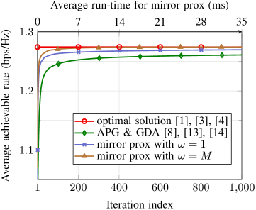
Figure 1: Convergence performance of Algorithm 1, GDA, APG averaged over $100$ channels. The simulation parameters taken are $M=150,L=50,$ and $D=1$.

We can see that Algorithm 1 based on the MP method has better objective than GDA and APG. Also, Algorithm 1 takes lesser number of iterations. Thus, GDA and APG [9] are not suitable for the applications where a fast convergence rate is required. Note that APG presented in [9] is essentially an approximate solution. On the other hand, Algorithm 1 is an exact method and thus can reach the optimal solution at convergence as clearly seen in Fig. 1. Note that we also demonstrate the impact of introducing $\omega$ when reformulating ($\mathcal{P}_{2}$) into ($\mathcal{P}_{4}$). As can be observed clearly, a proper value of $\omega$ can indeed speed up the convergence of Algorithm 1 very significantly. By extensive simulation settings, we find that $\omega=M$ yields a good convergence rate for Algorithm 1 overall, which is shown in Fig. 1. Further, we remark that the proposed algorithm converges within $500$ iterations. Also, the average run-time per iteration is very small, as shown in Fig. 1.

The main advantage of Algorithm 1 over second-order methods in [1, 3, 4] is that each iteration of Algorithm 1 is very memory efficient and computationally cheap, and hence, can be executed very fast. To demonstrate this, we compare the run-time of Algorithm 1 with the bisection method with LP in [1], both normalized to the run-time of the GP approach in [4, 3] for solving ($\mathcal{P}_{2}$) in Fig. 2. This shows the factor at which a particular method is faster than the GP method with normalized run-time of 1. We run the codes on a $64$-bit Windows operating system with $16$ GB RAM and Intel CORE i$7$, $3.7$ GHz. All iterative methods are terminated when the difference of the objective for the latest two iterations is less than $10^{-4}$. We observe that solving ($\mathcal{P}_{2}$) using a bisection search with LP is faster than converting it to a single GP, which is then solved by a dedicated GP solver. Most importantly, Algorithm 1 is 40 times faster than the LP method and approximately 100 times faster than the GP approach as shown in Fig. 2.

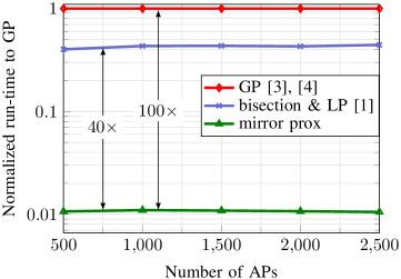
Figure 2: Comparison of run-time (in seconds) between Algorithm 1 and the bisection-based method for $L=40$.

In the next experiment, we investigate cell-free massive MIMO for large-scale scenarios. Instead of solving a generalized eigenvalue problem to find $\mathbf{q}_{l}^{*}$ as suggested in [3, 4] which incurs a complexity of $O(M^{3})$, we can reduce this complexity to $O(M^{2})$ using the method in [9, Appendix]. This complexity reduction and the low complexity of Algorithm 1 indeed allow us to investigate the performance of uplink large-scale cell-free massive MIMO, which has never been reported previously. In particular, we plot the cumulative distribution function (CDF) of the per-user achievable rate for $100$ channel realizations in Fig. 3. Three large-scale scenarios detailed in the caption of Fig. 3 are considered. Note that the AP-density, defined as the number of APs per $\text{\,}{\mathrm{km}}^{2}$ of area, is the same for all three scenarios. In particular, we compare the CDF of the per-user rate where both receiver filtering and power control are considered (i.e. alternately computing (6) and running Algorithm 1 until convergence, referred to as AO in the figure) to that where the power control only scheme (i.e. Algorithm 1) is adopted in which AP-weighting coefficients are all set to one.

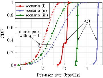
Figure 3: CDF of per-user achievable rate for three scenarios: (i) $M=500,L=50,D=1$, (ii) $M=2000,L=100,D=2$, and (iii) $M=2000,L=50,D=2$. Solid lines indicate the CDF of the per-user rate using both power and receiver filtering control, and dashed lines represent the CDF of the per-user rate using power control only.

It can be seen from Fig. 3 that the system performance improves when the number of APs increases (even the AP-density is fixed). Let us discuss scenarios (i) and (iii) first. Although the AP density is the same for both scenarios, the user-density (defined as the number of users per $\text{\,}{\mathrm{km}}^{2}$ of area) for scenario (iii) is much smaller than that for scenario (i), and hence, users in scenario (iii) suffer less interference than users in scenario (i) do. Thus, users in scenario (iii) have higher rates than those in scenario (i). If we increase the number of users in scenario (iii) from $50$ to $100$ as in scenario (ii), then the user-density and thereby inter-user interference increase, which decreases the per-user rate accordingly. Furthermore, it is interesting to note that for scenarios (ii) and (iii), considering both power and receiver filtering control can deliver more universally good services to the users than the power control only scheme. However, this comes at the cost of extra complexity imposed by the computation of the receiver filter coefficients. Therefore, it is important to consider both the receiver coefficient design and power control problems for large-scale scenarios.

V Conclusion

In this paper, we have considered the max-min fairness problem for uplink cell-free massive MIMO. As in previous studies, we have decomposed the problem into the receiver filtering design problem and the power control problem. In particular, we have proposed a novel power control scheme based on the MP method. The numerical results have demonstrated that the proposed method is superior to other existing methods such as LP-based, GDA-based, and APG-based methods. More specifically, the proposed method achieves the same objective as these conventional schemes but in much lesser time. The proposed scheme has enabled us to investigate the performance of cell-free massive in large-scale scenarios. We have also numerically shown that the proposed solution provides better fairness among the users compared to the power control only scheme where AP-weighting coefficients are all set to one.

References

• [1] H. Q. Ngo, A. Ashikhmin, H. Yang, E. G. Larsson, and T. L. Marzetta, “Cell-free massive MIMO versus small cells,” IEEE Trans. Wireless Commun., vol. 16, no. 3, pp. 1834–1850, Mar. 2017.
• [2] J. Zhang, S. Chen, Y. Lin, J. Zheng, B. Ai, and L. Hanzo, “Cell-free massive MIMO: A new next-generation paradigm,” IEEE Access, vol. 7, pp. 99 878–99 888, Jul. 2019.
• [3] M. Bashar, K. Cumanan, A. G. Burr, M. Debbah, and H. Q. Ngo, “On the uplink max-min SINR of cell-free massive MIMO systems,” IEEE Trans. Wireless Commun., vol. 18, no. 4, pp. 2021–2036, Apr. 2019.
• [4] M. Bashar, K. Cumanan, A. G. Burr, H. Q. Ngo, and H. V. Poor, “Mixed quality of service in cell-free massive MIMO,” IEEE Commun. Lett., vol. 22, no. 7, pp. 1494–1497, Jul. 2018.
• [5] T. C. Mai, H. Q. Ngo, and T. Q. Duong, “Uplink spectral efficiency of cell-free massive MIMO with multi-antenna users,” in 2019 3rd Int. Conf. Recent Advances Signal Process., Telecommun. & Comput. (SigTelCom), Mar. 2019, pp. 126–129.
• [6] Y. Nesterov, “Smooth minimization of non-smooth functions,” Math. Program., vol. 103, pp. 127–152, May 2005.
• [7] M. Farooq, H. Q. Ngo, and L. N. Tran, “Accelerated projected gradient method for the optimization of cell-free massive MIMO downlink,” in 2020 IEEE 31st Annu. Int. Symp. Pers., Indoor and Mobile Radio Commun., Aug./Sep. 2020, pp. 1–6.
• [8] M. Farooq, H. Q. Ngo, E.-K. Hong, and L.-N. Tran, “Utility maximization for large-scale cell-free massive MIMO downlink,” IEEE Trans. Commun., vol. 69, no. 10, pp. 7050–7062, Oct. 2021.
• [9] M. Farooq, H. Q. Ngo, and L. Nam Tran, “A low-complexity approach for max-min fairness in uplink cell-free massive MIMO,” in 2021 IEEE 93rd Veh. Technol. Conf. (VTC2021-Spring), Apr. 2021, pp. 1–6.
• [10] A. Nemirovski, “Prox-method with rate of convergence $O(1/t)$ for variational inequalities with lipschitz continuous monotone operators and smooth convex-concave saddle point problems,” SIAM J. Optim., vol. 15, no. 1, pp. 229–251, 2004.
• [11] A. Juditsky and A. Nemirovski, “First order methods for nonsmooth convex large-scale optimization, II: utilizing problems structure,” Optim. Mach. Learn., vol. 30, no. 9, pp. 149–183, Mar. 2011.
• [12] Y. Chen and X. Ye, “Projection onto a simplex,” Univ. Florida Digit. Collections, Feb. 2011.
• [13] Y. Nesterov and A. Nemirovskii, Interior-Point Polynomial Algorithms in Convex Programming.   Soc. Ind. and Appl. Math., 1994.
• [14] G. M. Korpelevich, “The extragradient method for finding saddle points and other problems,” Matecon, vol. 12, pp. 747–756, 1976.
• [15] A. Nedić and A. Ozdaglar, “Subgradient methods for saddle-point problems,” J. Optim. Theory and Appl., vol. 142, no. 1, pp. 205–228, Mar. 2009.