Self-supervised 3D Object Detection fromMonocular Pseudo-LiDAR

Abstract

There have been attempts to detect 3D objects by fusion of stereo camera images and LiDAR sensor data or using LiDAR for pre-training and only monocular images for testing, but there have been less attempts to use only monocular image sequences due to low accuracy. In addition, when depth prediction using only monocular images, only scale-inconsistent depth can be predicted, which is the reason why researchers are reluctant to use monocular images alone. Therefore, we propose a method for predicting absolute depth and detecting 3D objects using only monocular image sequences by enabling end-to-end learning of detection networks and depth prediction networks. As a result, the proposed method surpasses other existing methods in performance on the KITTI 3D dataset. Even when monocular image and 3D LiDAR are used together during training in an attempt to improve performance, ours exhibit is the best performance compared to other methods using the same input. In addition, end-to-end learning not only improves depth prediction performance, but also enables absolute depth prediction, because our network utilizes the fact that the size of a 3D object such as a car is determined by the approximate size.

I INTRODUCTION

Recognizing geometric features as well as semantic entities of the surrounding environment is essential for intelligent agents to output meaningful information [1]. Since the most important thing for detailed technology operation is to detect the position and state of an object in 3D, sensors that measure depth information, such as a stereo camera, RGBD camera, and 3D LiDAR sensor, are essential [2].

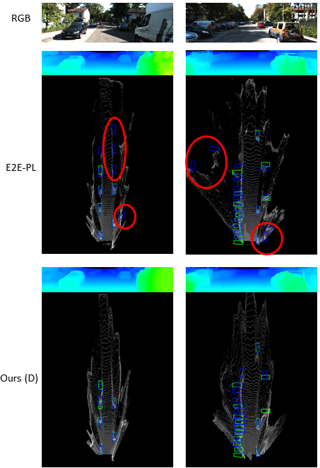
Figure 1: Depth estimation results and 3D object detection results of E2E-PL [3] and Ours (D) to the corresponding RGB images. False positives incorrectly detected by E2E-PL of cars on the road are circled in red. Green - correct answer label, blue - predicted result.

However, these sensors are expensive, and the amount of data sets on the market is absolutely insufficient. Moreover, contrary to the expectation that the 3D object recognition performance would be improved by using the image and LiDAR data together, the performance when using the LiDAR alone is much better. Therefore, the barriers to overcome for 3D object recognition for autonomous driving are: 1) the high price of high-performance 3D sensors, 2) the absence of prior research on 3D object detection, and 3) fusion is impossible due to the gap between the 2D sensor and the 3D sensor.

The goals of this study are as follows. First, we propose a monocular image-based algorithm to reduce the cost of the sensor and provide extensibility to experiment with larger datasets. In PL [4], also a method of using a monocular image as an input was suggested, but it is not possible to perform end-to-end learning. Mono PL [5] capable of end-to-end learning was developed, but in either case, it cannot be said that only monocular images are used perfectly. PL and Mono PL use DORN [6] as a depth estimation method because DORN networks have already used LiDAR information for pre-training. However, since our proposed depth estimation network uses self-supervised loss, it is possible to learn from only monocular images without LiDAR data even during pre-training and end-to-end learning. Second, we propose a method to improve the mono-based 3D object detection performance. Only monocular images are used as input, but additional experiments to obtain supervised loss from LiDAR are also conducted to achieve state-of-the-art performance.

Moreover, we propose three loss calculation methods. The first one is a method of calculating unsupervised loss from monocular images of three sequential frames (M). In this case, only moncular image input is used, and learning is possible without using LiDAR data in any case of pre-training. The second one is a method that uses both images and LiDAR (D). The supervised loss can be calculated from LiDAR. The last one is a method that uses all of the aforementioned losses (MD).

As a result, we significantly reduce the performance difference between mono-based and stereo-based algorithms. Among the models proposed by us, the self-supervised model (M) exhibits SOTA performance exceeding the existing mono-based algorithms [7, 8, 9, 10, 11] in the car category of the KITTI 3D validation dataset, assuring a large performance gap especially when IoU = 0.5. The supervised model (D) records SOTA performance in the moderate and hard difficulty levels in the car category of the KITTI 3D validation dataset.

In addition, the proposed method enables absolute depth estimation from monocular images. In the case of the conventional mono depth estimation, only the relative disparity could be estimated. However, since our method learns the object detection loss in 3D along with the depth estimation network, we are able to estimate the absolute depth on a consistent scale by learning the geometrical assumption. Mono PL[5] places additional limitations to solve the problem of local misalignment of PL and long-tail of the point cloud of object boundaries. But, our algorithm, through end-to-end learning, allows the network to estimate the depth at which it naturally leads to a 3D object detection.

In summary, the contribution of this paper is as follows.

• We propose a method to train with self-supervised loss using only monocular image sequences, which outperforms previous algorithms by more than 3% $AP_{BEV}$ at IoU = 0.5.

• In the case of fusing monocular image sequences and LiDAR together during training, we record SOTA performance in moderate and hard difficulty levels in the car category of the KITTI 3D validation dataset.

• Through end-to-end learning, when estimating depth from monocular image, it is possible to predict absolute depth, which was previously impossible.

• We narrow the performance gap between mono-based and stereo-based methods in detecting 3D objects.

II Related Works

II-A Depth Estimation

Supervised Depth Estimation. Eigen [12] first developed a network that can estimate depth from monocular images without special preprocessing. By proposing a coarse-to-fine network, it first extracts global features to predict the depth, and then improves the depth more precisely. DORN [6] learns by transforming depth information into ordinal regression through spacing-increasing discretization instead of learning with linear regression when estimating monocular depth.

Monocular Unsupervised Depth Estimation. Monodepth [13] estimates the depth by unsupervised learning by defining the image reconstruction loss to be the same as the original opposite image when projecting one stereo image to the opposite image with the predicted disparity. Monodepth2 [14] learns the camera pose through a separate network and improves the loss used in the existing Monodepth.

II-B 3D Object Detection

LiDAR-based Methods. Convolutional Neural Networks (CNNs) have been developed to process 2D images, and are not suitable for processing sparse 3D LiDAR data. Alternatively, to utilize the existing 2D CNN, PIXOR [15] projects the point cloud in two dimensions and processes it.

Image-based Methods. Multi-Level Fusion (MLF) [16] creates a point cloud by projecting RGB image pixels in 3D with pre-trained weights of Monodepth. The point cloud is then fused with RGB features to detect the 3D objects. Pseudo-LiDAR [4] developed MLF, which generates a point cloud with DORN and then passes it through the highest performing LiDAR-based 3D object detection algorithm. Since then, many pseudo-LiDAR-based studies have been derived.

Sensor Fusion Methods. SemanticVoxels [17] augment the point cloud by semantic features extracted from images. MonoDTR [18] adapt depth-aware transformer network [19] while fusing LiDAR data and image features.

III Methodology

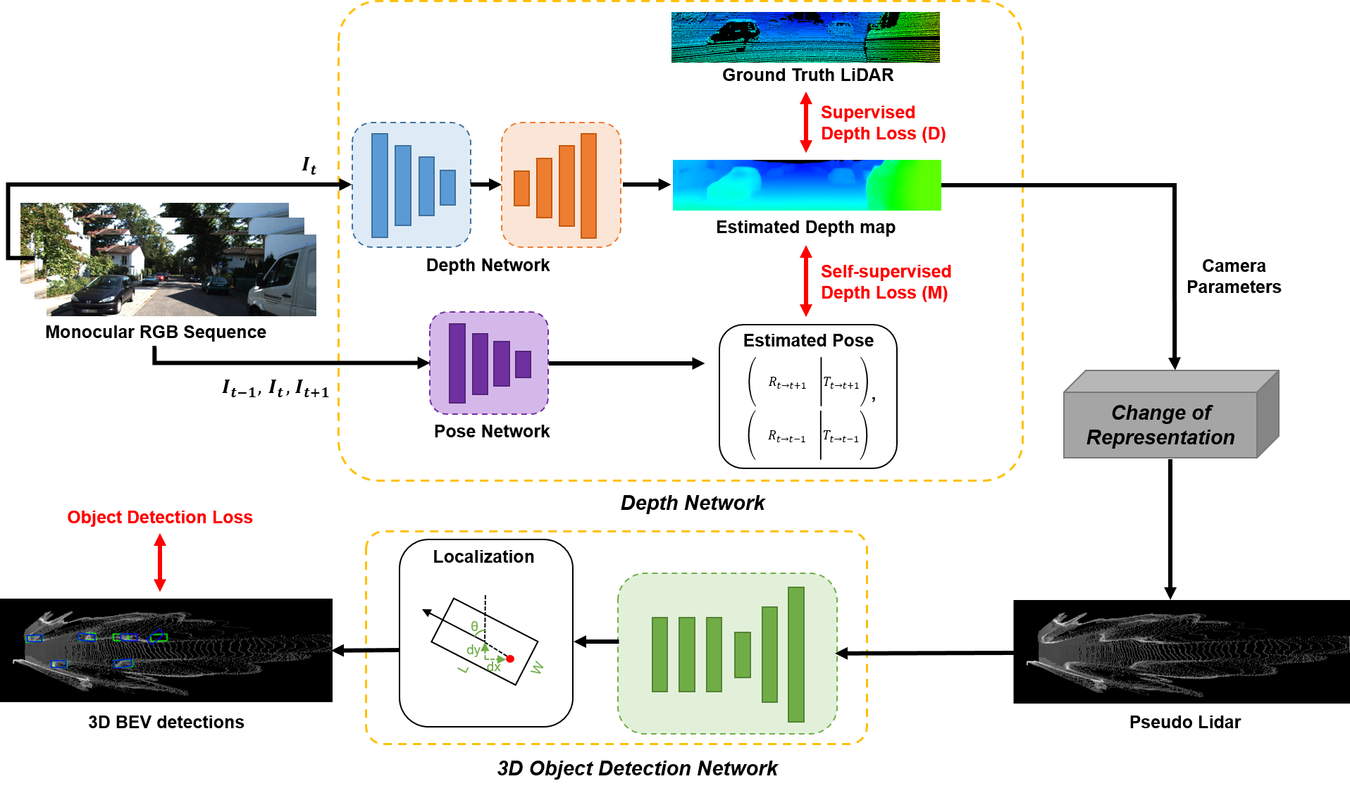
Figure 2: Our 3D object detection network. Three sequential images, $\bm{I}_{t-1}$, $\bm{I}_{t}$, $\bm{I}_{t+1}$ are used as inputs to estimate the camera pose, while the depth network feeds only $\bm{I}_{t}$. Learning with supervised loss (D) or self-supervised loss (M) or both (MD) are available, and the predicted depth is converted into a pseudo-LiDAR from through a change of representation scheme proposed by [3]. Then the 3D object network detects 3D objects by considering it as a LiDAR sensor measurement result.

III-A Overview

Fig. 2 displays the overall architecture of the proposed monocular 3D object detection framework. The framework consists of three main components: 1) monocular depth estimation, 2) PL point cloud generation, and 3) 3D object detection. First, the input monocular images pass through the monocular depth estimation module. For both supervised and self-supervised learning settings, only the center image ($\bm{I}_{t}$) gets fed into the depth network and becomes an estimated depth map. For self-supervised learning, the pose network receives two other temporal frames ($\bm{I}_{t-1}$ and $\bm{I}_{t+1}$) and estimates the relative camera motion. The depth estimation module can learn the estimation with supervision signals from geometric constraints (M) or ground-truth depths (D) or both (MD). Next, the PL point cloud generation module converts the estimated depth map into a PL point cloud in a way that gradients can propagate through the PL cloud. According to the 3D object detector that follows, the PL point cloud further gets either quantized (voxelized) or subsampled. Finally, the 3D object detection module performs 3D object detection on the PL point cloud.

III-B Scale-aware Depth Estimation

Due to the inherent scale ambiguity of monocular depth estimation, the process of monocular 3D object detection could become unstable. To deal with this, we propose a scale-aware depth estimation method. The key to overcoming the scale ambiguity is to represent depths as follows:

$$\hat{d}=\frac{\bar{D}_{\text{prior}}}{\sigma_{\text{min}}+(\sigma_{\text{max}}-\sigma_{\text{min}})\cdot x},$$ (1)

where $x\in[0,1)$ denotes the output of the depth network (disparity), $\sigma_{\text{max}}$ and $\sigma_{\text{min}}$ are the maximum and minimum values disparity can take, respectively and $\bar{D}_{\text{prior}}$ represents a scaling factor. We scale the output of the depth network twice. The first scaling places the estimated depths inside the range of $(1/\sigma_{\text{max}},1/\sigma_{\text{min}}]$. This scaling effectively makes the estimated depth scale-consistent over multiple scenes [14]. Next, we incorporate prior knowledge into the depth estimation process in the form of the scaling factor ($\bar{D}_{\text{prior}}$). An appropriate choice of the scaling factor lets the estimated depths lie in a reasonable range when combined with the scale-consistent depth estimation. We can set the scaling factor either by an empirical study or by an inductive process.

III-C Change of Representation

PL Point Cloud. After the depth estimation module, each pixel coordinate $(u,v)$ with depth $d$ in the 2D image space becomes a point $\bm{p}=(x,y,z)$ in the 3D space as follows:

$$\begin{cases}z&=d,\\ x&=(u-C_{x})\cdot z/f,\\ y&=(v-C_{y})\cdot z/f,\end{cases}$$ (2)

where $(C_{x},C_{y})$ is the camera center and $f$ is the focal length. The resulting point cloud ($\bm{P}$) contains all the generated points: $P=\{p_{1},...,p_{N}\}$, where $N$ is the total number of generated points.

Soft Quantization. Quantization aims to voxelize the region of interest and represent it as a 3D or 3D tensors. Since hard quantization hardly propagates gradients, we adopt the soft quantization technique [3]. Soft quantization defines a 3D occupation tensor $\bm{T}$ of $M$ bins as follows:

$$\bm{T}(m)=T(m,m)+\frac{1}{|\mathcal{N}_{m}|}\sum_{m^{\prime}\in\mathcal{N}_{m}}\bm{T}(m,m^{\prime}),$$ (3)

where $m\in\{1,...,M\}$ is a bin in $\bm{T}$, $\mathcal{N}_{m}$ represents the set of neighbor bins of $m$ and

$$\bm{T}(m,m^{\prime})=\begin{cases}0&\text{if}\,\,|\bm{P}_{m^{\prime}}|=0,\\ \frac{1}{|\bm{P}_{m^{\prime}}|}\sum_{\bm{p}\in\bm{P}_{m^{\prime}}}e^{-\frac{\|\bm{p}-\bm{\hat{p}}_{m}\|^{2}}{\sigma^{2}}}&\text{if}\,\,|\bm{P}_{m^{\prime}}|>0,\end{cases}$$ (4)

where $\bm{\hat{p}}_{m}$ is the center of a bin $m$, $\bm{P}_{m}=\{\bm{p}\in\bm{P},\text{s.t.}\,\,m=\underset{m}{\mathrm{argmin}}||\bm{p}-\hat{\bm{p}}_{m}^{\prime}||^{2}\}$ is the set of points inside the bin $m$.

III-D Loss Functions

Depth Smoothness Loss. We impose the depth smoothness loss on the estimated depth map to restrain random sharp lines [20]. The smoothness loss regularizes the gradients of the estimated depth map ($\bm{\hat{D}}_{t}$). Moreover, we penalize the smoothness loss by inversely weighting it with the gradients of the input monocular image so that essential gradients would remain. Finally, the smoothness loss is

$$L_{smooth}=\sum|\partial_{x}\hat{\bm{D}}_{t}|\cdot e^{-|\partial_{x}\bm{I}_{x}|}+|\partial_{y}\hat{\bm{D}}_{t}|\cdot e^{-|\partial_{y}\bm{I}_{y}|}.$$ (5)

Supervised Depth Loss (D). LiDAR signals provide direct supervision signals for depth learning. We formulate a $L_{1}$ loss for depth supervision by projecting 3D LiDAR signals to the 2D image space and comparing the projected depth map ($\bm{D}_{t}$) and the estimated depth map ($\bm{\hat{D}}_{t}$). In addition, we filter out the loss with a mask representing the pixels where a LiDAR signal exists since LiDAR signals are sparse. Finally, we define the loss as follows:

$$L_{D}=\|\mathbbm{1}_{\{\bm{D}_{t}>0\}}\cdot(\bm{D}_{t}-\hat{\bm{D}}_{t})\|_{1},$$ (6)

where $\mathbbm{1}_{S}$ is an indicator function for a set $S$.

Self-Supervised Depth Loss (M). The photometric consistency loss [21] takes a central role in training the depth network with unlabeled temporal images. The loss restores the center image ($\bm{I}_{t}$) from two nearby views ($\bm{I}_{t-1}$ and $\bm{I}_{t+1}$) using the estimated motion vectors ($\hat{\bm{T}}$) and the predicted depth map ($\hat{\bm{D}}_{t}$); enforces photometric consistency by minimizing the photometric error. For the reconstruction, we project each pixel in $\bm{I}_{t}$ onto the nearby views as follows:

$$p_{n\rightarrow t}=\hat{\bm{K}}\cdot\hat{\bm{T}}_{t\rightarrow n}\cdot\hat{\bm{D}_{t}}(p_{t})\cdot\hat{\bm{K}}^{-1}\cdot p_{t},$$ (7)

where $n\in\{t-1,t+1\}$, $\hat{\bm{K}}$ is the estimated camera intrinsic matrix, $\hat{\bm{T}}$ is an element in the special Euclidean group SE(3) consisting of a rotation matrix $\bm{R}\in\mathbb{R}^{3\times 3}$ and a translation vector $\bm{t}\in\mathbb{R}^{3}$) and $p_{t}$ represents the homogeneous coordinate of each pixel in $\bm{I}_{t}$. Finally, we evaluate the photometric consistency loss as $pe(\bm{I}_{t},\bm{\hat{I}}_{n\rightarrow t})$, where

$$pe(\bm{I}_{a},\bm{I}_{b})=\frac{\alpha}{2}(1-SSIM(\bm{I}_{a},\bm{I}_{b}))+(1-\alpha)\|\bm{I}_{a}-\bm{I}_{b}\|_{1},$$ (8)

where $\alpha=0.85$ and SSIM is the structural similarity measure [22].

Combined Depth Loss (MD). When using both the supervised and self-supervised depth losses, we make the two losses complementary to each other using two masks as follows:

$$L_{MD}=\lambda_{M}(\mathbbm{1}_{\{L_{D}=0\}}\cdot L_{M})+\lambda_{D}(\mathbbm{1}_{\{L_{D}>0\}}\cdot L_{D}),$$ (9)

where $\lambda_{M}$ and $\lambda_{D}$ are weighting factors.

3D Detection Loss. We utilize two loss functions for learning 3D object detection: the focal loss for classification and the smooth L1 loss for 3D bounding box regression. The focal loss improves the learning efficiency when there exists class imbalance in the training data; the point clouds for 3D object detection in general contain more points belonging to background than objects. The smooth L1 loss prevents outliers from deteriorating gradients and stabilizes the regression learning.

IV Experiments

IV-A Settings

Dataset. We evaluate the performance of 3D object detection on the challenging KITTI 3D object detection benchmark [23]. The KITTI 3D benchmark consists of 7,481 images with ground-truth 3D labels. The ground-truth labels comprise of three categories: easy, moderate and hard. We split the data into 3,712 training and 3,769 validation images. In our algorithm, an image sequence is required to obtain unsupervised loss, but the KITTI 3D dataset does not provide continuous images. The previous and next frames of the KITTI 3D image are obtained from the KITTI raw dataset. In this process, if the KITTI 3D image is the first frame or the last frame of the video sequence, it is not included in the training and testing because there are no previous and subsequent frames. Excluded images are 7 in the training set and 8 in the validation set, which are not expected to significantly affect performance.

TABLE I: Comparison of the car category on the KITTI validation set with existing mono-based studies.

Method	Reference	Input	$\textbf{AP}_{\textbf{BEV}}$ , IoU=0.5			$\textbf{AP}_{\textbf{BEV}}$ , IoU=0.7
		(+ pretrained input)	Easy	Moderate	Hard	Easy	Moderate	Hard
MonoGRNet[7]	AAAI 2019	Mono	54.21	39.69	33.06	24.97	19.44	16.30
MonoPair[8]	CVPR 2020	Mono	61.06	47.63	41.92	24.12	18.17	15.76
Monodle[9]	CVPR 2021	Mono	59.78	45.84	41.60	23.97	19.23	16.70
GUPNet[10]	ICCV 2021	Mono	61.78	47.06	40.88	31.07	22.94	19.75
Homo[11]	CVPR 2022	Mono	-	-	-	31.04	22.99	19.84
Ours(M)	-	Mono	64.35	50.39	44.03	28.25	23.19	21.01
PL-MONO[4]	CVPR 2019	Mono(+LiDAR)	70.8	49.4	42.7	40.6	26.3	22.9
Mono PL[5]	ICCVW 2019	Mono(+LiDAR)	72.1	53.1	44.6	41.9	28.3	24.5
DD3D[24]	ICCV 2021	Mono, Depth	-	-	-	37.0	29.4	25.4
MonoDTR[18]	CVPR 2022	Mono, LiDAR	69.04	52.47	45.90	33.33	25.35	21.68
Ours(D)	-	Mono, LiDAR	70.86	60.23	54.54	37.42	31.05	29.13

IV-B Implementation Details

The pre-trained parameters provided by Monodepth2 are used for the depth estimation network, and the resolution of the input and output is set to 640 $\times$ 192. In the case of end-to-end learning, unlike the existing Monodepth2, multi-scale learning by adjusting the input image to various sizes is not performed, and a resolution of 308 $\times$ 1248 is used.

To generate the input of the 3D object detection network, the scale-aware depth map, which is the result of the depth estimation network, is converted into a pseudo-LiDAR using soft quantization. The existing PIXOR network is borrowed for 3D object detection. Since PIXOR converts the 3D LiDAR point cloud into a bird’s eye view (BEV) expression viewed from above, the generated Pseudo-LiDAR is converted to the BEV format and then passed through the PIXOR network.

End-to-end learning is implemented with PyTorch, and most hyperparameters followed E2E-PL. Adam Optimizer is used, and the learning rate is multiplied by 0.1 every 10 steps from 0.001. For a total of 15 epoch training, the supervised learning model (D), the self-supervised learning model (M), and the model using both (MD) using 4 Titan Xp with a batch size of 6 took 5.5, 6, and 7 hours, respectively.

IV-C Results and Analysis

The main results are summarized in Table I. Our model (M), trained self-supervised using only monocular images, performed the best in the car category of all difficulty levels, and our model (D), using monocular images and 3D LiDAR together, performed in the car category of medium and hard difficulty levels. The highest $AP_{BEV}$ performance is achieved in both IoU = 0.5 and IoU = 0.7. This result confirms the possibility to predict the depth consistent with the scale.

Effect of Depth loss. The results of the depth prediction experiments for the three loss types are shown in Table II. The depth estimation evaluation method followed [12], and the validation set of KITTI 3D [23] data is evaluated. MD2 stands for Monodepth2 [14], PIXOR^∗ denotes PIXOR [15] with soft quantization applied, and E2E stands for end-to-end learning. The performance of the end-to-end trained model using MD and D losses is better than the result of learning only with Monodepth2, and again, the model (D) using 3D LiDAR exhibited the best results.

Scale-aware Depth Estimation. Table III shows 3D object detection performance according to end-to-end learning and three loss types. The performance of the existing PIXOR [15] using 3D LiDAR is the highest. After learning Monodepth2 and PIXOR individually, the result of simply connecting them is not so good. In Table II, we compare the performance with and without adopting scale-aware depth estimation. This shows that inconsistency exists in the depth predicted by the prediction model, and it is very far from the actual depth. However, when end-to-end learning is performed only with unsupervised loss (M), the performance increased nearly 7 times, showing the effect of end-to-end learning. The 3D object detection result also showed the highest performance in the model (D) using 3D LiDAR.

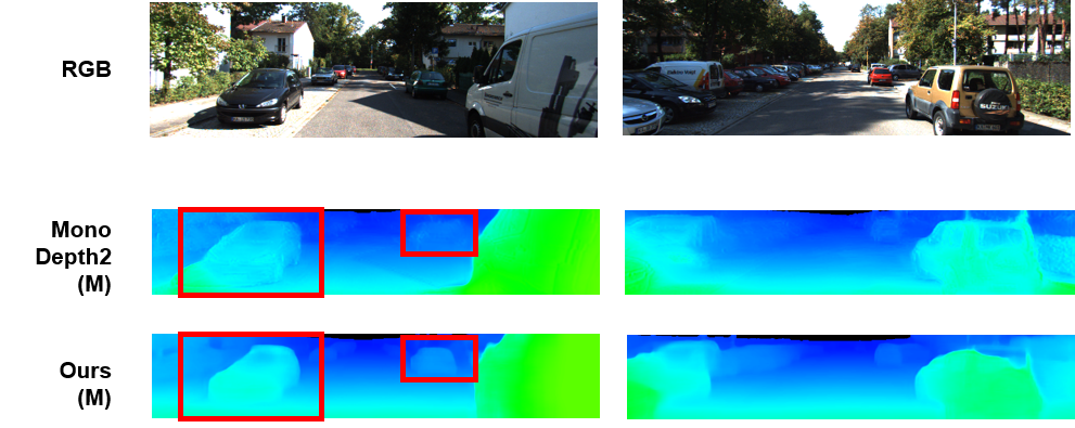
Figure 3: Comparison of depth estimation results of Monodepth2 [14] and Ours (M)

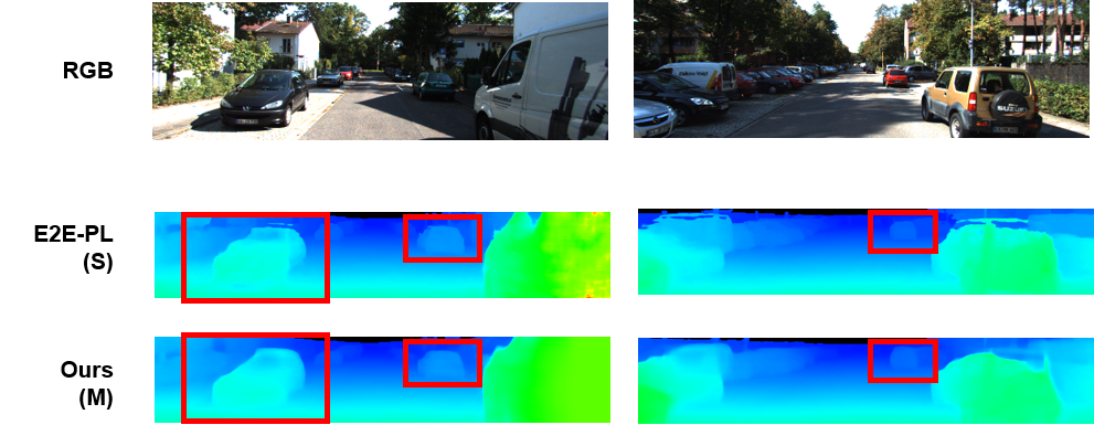
Figure 4: Comparison of depth estimation results of E2E-PL [3] and Ours (M).

TABLE II: Depth estimation performance according to loss types and with or without Scaled Depth.

Method	Train	Scaled Depth	$AbsRel$	$SqRel$	$RMSE$	$RMSE_{log}$	$\delta<1.25$	$\delta<1.25^{2}$	$\delta<1.25^{3}$
MD2	M	-	0.234	2.101	8.267	0.400	0.583	0.787	0.891
MD2+PIXOR∗+E2E	M	no	0.997	16.475	20.569	6.091	0.000	0.000	0.000
MD2+PIXOR∗+E2E	M	yes	0.313	4.906	10.418	0.361	0.602	0.817	0.919
MD2+PIXOR∗+E2E	MD	yes	0.111	0.780	4.503	0.191	0.868	0.958	0.984
MD2+PIXOR∗+E2E	D	yes	0.107	0.736	4.415	0.186	0.872	0.960	0.984

TABLE III: 3D object detection result according to end-to-end learning and loss types.

Method	Train	$\textbf{AP}_{\textbf{BEV}}$ (%), IoU=0.5			$\textbf{AP}_{\textbf{BEV}}$ (%), IoU=0.7
		Easy	Moderate	Hard	Easy	Moderate	Hard
MD2+PIXOR∗	M	8.73	6.93	5.36	4.55	4.55	4.55
MD2+PIXOR∗+E2E	M	64.35	50.39	44.03	28.25	23.19	21.01
MD2+PIXOR∗+E2E	MD	69.85	58.83	53.72	37.02	31.00	29.26
MD2+PIXOR∗+E2E	D	70.86	60.23	54.54	37.42	31.05	29.13

Comparative Study. The depth estimation results of E2E-PL and our method and the 3D object detection results are visualized in Figure 1. In the case of E2E-PL, it is outputting much more predictions than 3D object labels. On the other hand, our proposed method outputs the number of predictions that closely match the label, so the number of false positives is significantly less than that of E2E-PL.

In Fig. 3, we qualitatively compare the depth estimation results of Monodepth2 [14] and our proposed method. Monodepth2 is not able to accurately detect distant objects or mistook image features such as shadows for depth in many cases. In particular, in the first picture, the shadow of the roof of the house reflected on the floor still exists at the depth predicted by Monodepth2. However, our method is accurately predicting the depth.

Also, in Fig. 4, we compare the depth estimation results of E2E-PL [3] with our method (M). Since E2E-PL uses stereo images and 3D LiDAR, its performance is inevitably superior to that of monocular images alone, but our algorithm nevertheless shows similar depth estimation performance to E2E-PL.

We quantitatively compare the performance of our proposed method with existing monocular image-based methods. Because we used PIXOR as the 3D object detection network, we could only evaluate $AP_{BEV}$ (%), and the results can be seen in Table I. As a result of comparing algorithms using only monocular images, our result, which is trained with unsupervised loss (M), outperformed most difficulty levels of the KITTI 3D validation set and showed the best performance. As a result of learning with supervised loss (D), our proposed method shows the SOTA performance in moderate and hard difficulty levels of car category in the KITTI 3D validation set.

V Conclusion

In this paper, we proposed a network that learns with self-supervised loss using only monocular image sequences. The proposed monocular depth estimation network with a consistent scale is trained through end-to-end learning. The proposed network improved the performance of the monocular-based method in detecting 3D objects and narrowed the performance gap with the stereo-based method.

Despite these advances, the monocular image-based method is still less accurate than the LiDAR-based method by about 10% $AP_{BEV}$. Also, as we use reduced image size to 640$\times$192 when inputting to the network, there is a problem in that a distant object is expressed in a small size in the image, making it more difficult to detect. In addition, if there is a moving object in the image sequence, an inaccurate unsupervised loss is calculated. In the future, we will study further how to isolate the pixels corresponding to moving objects and treat them differently by generating binary masks and attention map.

References

- [1] U.-H. Kim, S.-H. Kim, and J.-H. Kim, “Simvodis++: Neural semantic visual odometry in dynamic environments,” IEEE Robotics and Automation Letters, vol. 7, no. 2, pp. 4244–4251, 2022.
- [2] U.-H. Kim, S.-H. Kim, and J.-H. Kim, “Simvodis: Simultaneous visual odometry, object detection, and instance segmentation,” IEEE Transactions on Pattern Analysis and Machine Intelligence, vol. 44, no. 1, pp. 428–441, 2022.
- [3] R. Qian, D. Garg, Y. Wang, Y. You, S. Belongie, B. Hariharan, M. Campbell, K. Q. Weinberger, and W.-L. Chao, “End-to-end pseudo-lidar for image-based 3d object detection,” in CVPR, 2020.
- [4] Y. Wang, W.-L. Chao, D. Garg, B. Hariharan, M. Campbell, and K. Q. Weinberger, “Pseudo-lidar from visual depth estimation: Bridging the gap in 3d object detection for autonomous driving,” in CVPR, 2019.
- [5] X. Weng and K. Kitani, “Monocular 3d object detection with pseudo-lidar point cloud,” in ICCV Workshops, 2019.
- [6] H. Fu, M. Gong, C. Wang, K. Batmanghelich, and D. Tao, “Deep Ordinal Regression Network for Monocular Depth Estimation,” in CVPR, 2018.
- [7] Z. Qin, J. Wang, and Y. Lu, “Monogrnet: A geometric reasoning network for 3d object localization,” in AAAI, 2019.
- [8] Y. Chen, L. Tai, K. Sun, and M. Li, “Monopair: Monocular 3d object detection using pairwise spatial relationships,” in CVPR, 2020.
- [9] X. Ma, Y. Zhang, D. Xu, D. Zhou, S. Yi, H. Li, and W. Ouyang, “Delving into localization errors for monocular 3d object detection,” in CVPR, 2021.
- [10] Y. Lu, X. Ma, L. Yang, T. Zhang, Y. Liu, Q. Chu, J. Yan, and W. Ouyang, “Geometry uncertainty projection network for monocular 3d object detection,” in ICCV, 2021.
- [11] J. Gu, B. Wu, L. Fan, J. Huang, S. Cao, Z. Xiang, and X.-S. Hua, “Homography loss for monocular 3d object detection,” in CVPR, 2022.
- [12] D. Eigen, C. Puhrsch, and R. Fergus, “Depth map prediction from a single image using a multi-scale deep network,” in NeurIPS, 2014.
- [13] C. Godard, O. M. Aodha, and G. J. Brostow, “Unsupervised monocular depth estimation with left-right consistency,” in CVPR, 2017.
- [14] C. Godard, O. M. Aodha, M. Firman, and G. Brostow, “Digging into self-supervised monocular depth estimation,” in ICCV, 2019.
- [15] B. Yang, W. Luo, and R. Urtasun, “Pixor: Real-time 3d object detection from point clouds,” in CVPR, 2019.
- [16] B. Xu and Z. Chen, “Multi-level fusion based 3d object detection from monocular images,” in Proceedings of the IEEE conference on computer vision and pattern recognition, pp. 2345–2353, 2018.
- [17] J. Fei, W. Chen, P. Heidenreich, S. Wirges, and C. Stiller, “Semanticvoxels: Sequential fusion for 3d pedestrian detection using lidar point cloud and semantic segmentation,” in 2020 IEEE International Conference on Multisensor Fusion and Integration for Intelligent Systems (MFI), 2020.
- [18] K.-C. Huang, T.-H. Wu, H.-T. Su, and W. H. Hsu, “Monodtr: Monocular 3d object detection with depth-aware transformer,” in CVPR, 2022.
- [19] A. Vaswani, N. Shazeer, N. Parmar, J. Uszkoreit, L. Jones, A. N. Gomez, L. u. Kaiser, and I. Polosukhin, “Attention is all you need,” in NeurIPS, 2017.
- [20] R. Mahjourian, M. Wicke, and A. Angelova, “Unsupervised learning of depth and ego-motion from monocular video using 3d geometric constraints,” in CVPR, 2018.
- [21] T. Zhou, M. Brown, N. Snavely, and D. G. Lowe, “Unsupervised learning of depth and ego-motion from video,” in CVPR, 2017.
- [22] Z. Wang, A. C. Bovik, H. R. Sheikh, and E. P. Simoncelli, “Image quality assessment: from error visibility to structural similarity,” IEEE transactions on image processing, vol. 13, no. 4, pp. 600–612, 2004.
- [23] A. Geiger, P. Lenz, C. Stiller, and R. Urtasun, “Vision meets robotics: The kitti dataset,” The International Journal of Robotics Research, vol. 32, no. 11, pp. 1231–1237, 2013.
- [24] D. Park, R. Ambrus, V. Guizilini, J. Li, and A. Gaidon, “Is pseudo-lidar needed for monocular 3d object detection?,” in ICCV, 2021.