Numerical Simulation of Hot Accretion Flow around Bondi Radius

Abstract

Previous numerical simulations have shown that strong winds can be produced in the hot accretion flows around black holes. Most of those studies focus only on the region close to the central black hole, therefore it is unclear whether the wind production stops at large radii around Bondi radius. Bu et al. 2016 studied the hot accretion flow around the Bondi radius in the presence of nuclear star gravity. They find that when the nuclear stars gravity is important/comparable to the black hole gravity, winds can not be produced around the Bondi radius. However, for some galaxies, the nuclear stars gravity around Bondi radius may not be strong. In this case, whether winds can be produced around Bondi radius is not clear. We study the hot accretion flow around Bondi radius with and without thermal conduction by performing hydrodynamical simulations. We use the virtual particles trajectory method to study whether winds exist based on the simulation data. Our numerical results show that in the absence of nuclear stars gravity, winds can be produced around Bondi radius, which causes the mass inflow rate decreasing inwards. We confirm the results of Yuan et al. which indicates this is due to the mass loss of gas via wind rather convectional motions.

1 Introduction

Hot accretion flow with low mass accretion rate is an important and distinguished class of accretion disks. Compared to the well-known standard thin disk (cold accretion mode), hot accretion flow has a lower density, as well as higher temperature and scale height. Consequently, the radiative efficiency drops dramatically so this model is called radiatively inefficient accretion flow (RIAF). Hot accretion flow model is arguably the standard model of low-luminosity active galactic nuclei (LLAGNs) in the majority of galaxies in the nearby universe (see e.g. Ho 2008; Antonucci 2012), and the hard/quiescent states of black hole X-ray binaries (BHXBs) as well (see, e.g. Narayan & McClintock 2008; Belloni 2010; Yuan & Narayan 2014).

Discovery of strong wind is one of the most important advantages in our understanding of hot accretion flows in recent years (see, e.g., Stone et al. 1999; Stone & Pringle 2001; Yuan et al. 2012a, b; Narayan et al. 2012; Li et al. 2013; Gu 2015; Yuan et al. 2015). The existence of wind in hot accretion flow is also confirmed by the 3 Ms Chandra observation of the supermassive black hole (SMBH) in our galactic centre, Sgr A* (Wang et al. 2013). Wind not only plays a significant role in AGN feedback (e.g., Ostriker et al. 2010) but it also brings us important insights and questions regarding the physics of the black hole accretion.

Yuan et al. 2015 had extensively studied the properties of wind including terminal velocity and mass flux of the wind for the hot accretion flow at small scale, $r<10^{3}r_{\rm s}$, where $r_{\rm s}$ is the Schwarzschild radius. They used virtual trajectory test particle method. In principle, a trajectory is obtained by connecting the positions of the same test particle at different times. This concept is related to the Lagrangian description of fluid and is different from the streamline. Based upon this method they showed that the mass accretion rate decreases inward due to mass loss of wind rather than convection. According to their results, the poloidal velocity of wind roughly follows $v_{\rm p,wind}\approx(0.2-0.4)v_{\rm{}_{K}}(r)$, where $v_{\rm{}_{K}}(r)$ represents the Keplerian velocity at radius $r$. In addition, they found that the mass flux of wind can be described as

$$\dot{M}_{\rm wind}\approx\dot{M}_{\rm BH}(r/20r_{\rm s}),$$ (1)

where $\dot{M}_{\rm BH}$ is the mass accretion rate at the black hole horizon. The above equation mainly means that the wind comes from large radii. Therefore, the important question will be: how far the wind can be produced? or equivalently, where is the upper limit of the radius that the equation (1) can be applied to?

To answer such questions, we first need to introduce some physical radii related to the accretion process. For the spherically symmetric flow, in the absence of the rotation and radiation, the Bondi radius (Bondi 1952) will be defined as,

$$r_{\rm{}_{B}}=\frac{GM}{c_{\rm s,\infty}^{2}},$$ (2)

where $M$ is the black hole mass, $G$ is the gravitational constant, and $c_{\rm s,\infty}$ represents the sound speed of the gas at infinity. From this radius towards the black hole the negative gravitational energy dominates over the thermal energy of the gas. However, in real accretion flow, the gas has some amount of angular momentum and rotates around the central black hole. Therefore, we can define a characteristic radius at which the centrifugal and gravitational forces balance each other. The centrifugal radius is given as,

$$r_{\rm{}_{C}}=\frac{\ell^{2}}{GM},$$ (3)

where $\ell$ is the angular momentum per unit mass. This radius is larger than Schwarzschild radius and can be less than Bondi one, i.e., $r_{\rm s}\ll r_{\rm{}_{C}}<r_{\rm{}_{B}}$. Existence of any mechanism for driving angular momentum tends to give rise the inflowing gas form a rotating accretion disc before falling down on to the black hole. It is well known that in a real accretion flow the angular momentum is transferred by Maxwell stress associated with Magnetohydrodynamic (MHD) turbulence driven by Magneto-rotational instability (MRI; Balbus & Hawley 1998). In hydrodynamical (HD) simulations, it is common to mimic the effect of the magnetic stress by adding viscosity terms for both driving angular momentum outwards as well as producing heat.

A good model for studying the dynamics and the structure of the accretion gas onto a SMBH should cover a wide range of spatial scales, from the inner region, where an accretion disc forms, to the the region outside the Bondi radius, where the accretion process originates in the first steps. So far, several HD and MHD simulations have been done to connect large and small scales (see, i.e., Proga & Begelman 2003a, b; Li et al. 2013; Bu et al. 2016a, b; Inayoshi et al. 2018, 2019). For instance, Bu et al. 2016a, b studied the accretion flow around Bondi radius. They found that by including the gravity of nuclear stars, the physics can be totally changed. More precisely, they showed that in the presence of nuclear star gravity, the winds can not be produced locally. They also did some tests and found that when the nuclear star gravity is excluded, the winds can be generated locally around Bondi radius. On the other hand, Inayoshi et al. 2018 performed two-dimensional HD simulations of hot accretion flow at a range about $10^{-2}r_{\rm{}_{B}}\leq r\leq 50r_{\rm{}_{B}}$. They found a global steady accretion solution with two distinguished regimes: (1) the outer rotational equilibrium region around Bondi radius follows the density profile of $\rho\propto(1+r_{\rm{}_{B}}/r)^{3/2}$ with subsonic gas motion; (2) the inner solution where the geometrically thick torus follows $\rho\propto r^{-1/2}$. Based upon the density and the mass accretion rate ($\dot{M}\propto r$) profiles of inner part, they argued that the physical properties of this region are consistent with the convection-dominated accretion flow (CDAF) model proposed by Narayan et al. 2000. More precisely, since they did not find wind in their solutions, they claimed that the adiabatic inflow-outflow solution (ADIOS; Blandford & Begelman 1999, 2004; Begelman 2012) is not the main reason for decreasing mass accretion rate at such large radii. Therefore, they concluded that the convection causes the mass accretion rate decreases inward.

The motivations for performing the HD simulations of this paper are threefold. First, we want to check whether or not the inward decrease of mass accretion rate is due to the convection. The second purpose is to study the hot accretion flow at large radii to investigate how far the wind can move outward. The third motivation is the study of the effects of the thermal conduction on the wind. This is mainly because for systems with extremely low accretion rate, such as our galactic center Sgr A* and M87 galaxy, the accretion flows are weakly collisional. The electron collisional mean free path then can be much larger than its Larmor radius. Consequently, the conduction can significantly influence the dynamics of the accretion flow and transport energy from the inner to the outer regions (Johnson & Quataert 2007; Quataert 2008). In this paper, we revisit Inayoshi et al. 2018 by performing numerical HD simulations with some modifications to extensively study the detailed properties of wind at large radii. Following Yuan et al. 2015, we use the much more precise trajectory analysis of virtual test particles based on our simulation data to study whether does wind exist (see section 3.5 for more details).

The main structure of the paper is as follows. In Section 2, we will describe the basic HD equations, simulation method, and initial and boundary conditions. The results will be presented in Section 3 and we briefly overview of the trajectory method we use to analyze the simulation data (subsection 3.5). We then summarize our work in Section 4.

2 Method

We perform axisymmetric two-dimensional (2D) HD simulations using the publicly available numerical simulation package PLUTO , which is a finite-volume/finite-difference, shock-capturing code designed to integrate a system of conservation lows based on conservative Godunov scheme (Mignone et al. 2007). Our basic simulation setup builds upon Inayoshi et al. 2018, 2019. In the following subsections, we outline our numerical model and the differences from those aforementioned simulations.

2.1 Basic equations

To compute the structure and the evolution of an accretion flow with low mass accretion rate around SMBH at large radii, we solve the basic HD equations, including the equation of continuity,

$$\diff{\rho}{t}+\rho\nabla\cdot\bm{v}=0,$$ (4)

the momentum balance equation,

$$\rho\diff{\bm{v}}{t}=-\nabla p-\rho\nabla\psi+\nabla\cdot\bm{\sigma},$$ (5)

and the energy equation,

$$\rho\diff{e}{t}=-p\nabla\cdot\bm{v}+(\bm{\sigma}\cdot\nabla)\bm{v}-\nabla\cdot\bm{Q}.$$ (6)

In the above equations, $\rho$, $\bm{v}$, $p$, $\psi$, and $e$ are the density, velocity, gas pressure, gravitational potential, and internal energy per unit mass, respectively. Here, we only take into account the gravity of the central black hole and neglect the nuclear stars gravity. Therefore, the black hole potential can be adopted as $\psi=-GM/r$. $\bm{\sigma}$ is the viscous stress tensor and $\bm{Q}$ in the last term of the right-hand side of energy equation represents the thermal conduction. The radiative losses and AGN feedback are not considered in this study. The Lagrangian/comoving derivative presented in the first terms of the above set of equations is given by $\mathrm{d}/\mathrm{d}t\equiv\partial/\partial t+\bm{v}\cdot\nabla$. We assume the equation of state of ideal gas in the form of $p=\left(\gamma-1\right)\rho e$ and set $\gamma=5/3$.

In real accretion flow, the angular momentum is transferred by the Maxwell stress associated with MHD turbulence driven by MRI (Balbus & Hawley 1998). Although we do not include magnetic field in our HD simulations, we assume the viscous stress tensor, $\bm{\sigma}$, to mimic its effects for driving angular momentum and producing dissipation heat (see e.g., Yuan et al. 2012a; Bu et al. 2016a). The components of the viscous stress tensor are given by,

$$\sigma_{ij}=\rho\nu\left[\left(\frac{\partial v_{j}}{\partial x_{i}}+\frac{\partial v_{i}}{\partial x_{j}}\right)-\frac{2}{3}\left(\nabla\cdot\bm{v}\right)\delta_{ij}\right],$$ (7)

where $\nu$ is the kinematic viscosity coefficient and $\delta_{ij}$ is the usual Kronecker delta . We adopt the standard $\alpha$-prescription of viscosity (Shakura & Sunyaev 1973) as,

$$\nu=\alpha\frac{c_{\rm s}^{2}}{\Omega_{\mathrm{K}}},$$ (8)

where $\alpha$ is the viscosity parameter, $c_{s}$ is the sound speed, and $\Omega_{\mathrm{K}}(\equiv\sqrt{GM/r^{3}})$ is the Keplerian angular velocity. Following Inayoshi et al. 2018, the viscosity parameter is defined as,

$$\alpha=\alpha_{{}_{0}}\left\{\exp\left[-\left(\frac{\rho_{\rm crit}}{\rho}\right)^{2}\right]+{\rm max}\left(0,-\frac{\partial\ln\ell}{\partial\ln r}\right)\right\},$$ (9)

where $\alpha_{{}_{0}}$ is the strength of the viscosity and $\rho_{\rm crit}$ represents the threshold of the density above which the viscosity will be turned on (see equation (13) for more details). The second term in equation (9) is considered to achieve steady state accretion flow, since our 2D simulations cannot capture the three-dimensional (3D) effect of rotational instability. This form of the viscosity causes the viscous process becoming active in the disk region where the angular velocity has a significant fraction of the Keplerian, i.e., $r\lesssim r_{\rm{}_{C}}$.

Thermal conduction is also expected to modify the accretion flow structure significantly. Here, we explain the definition of thermal conduction which is present in models B and C (see table 1). As we mentioned in the introduction part, one of the purpose of this paper is to carry out simulations to study the effects of thermal conduction on wind at large radii. Motivated by the results of Sharma et al. 2008, for our runs with conduction, the thermal conduction term $-\nabla\cdot\bm{Q}$ is added to the right-hand side of the energy equation. In purely HD limit, the heat flux can be written as $\bm{Q}=-\kappa\nabla T$, where $\kappa$ is the thermal diffusivity. In a one-temperature structure, as in our case, temperature can be evaluated as $T=\mu m_{\rm p}p/(k_{\rm{}_{B}}\rho)$ where $k_{\rm{}_{B}}$ is the Boltzmann constant, $m_{\rm p}$ is the proton mass, and $\mu$ is the mean molecular weight. Following Sharma et al. 2008 and Bu et al. 2016 for the form of thermal diffusivity, we will adopt

$$\chi=\frac{\kappa T}{p}=\alpha_{\rm c}\sqrt{GMr},$$ (10)

where $\alpha_{\rm c}=[0.2-2]$ is the dimensionless conductivity. To prevent the conduction time step from being excessively short, we reduce the conductivity in the ambient medium. To do so, we limit the conductivity so that the time scale of conduction, $t_{\rm cond}=r^{2}/\chi$, would be longer than $0.1$ times the dynamical time-scale, $t_{\rm dyn}=(r^{3}/GM)^{1/2}$. This also can effectively mimic the effect of saturated conduction in extremely hot plasma regions.

2.2 Numerical method

To solve the system of equations (4)-(6), we adopt spherical polar coordinates ($r,\theta,\phi$). Simulation settings are almost the same as those in Inayoshi et al. 2018, 2019 except some modifications explained in this subsection. For all the runs presented here, we assume the black hole mass as $M=10^{8}M_{\odot}$, where $M_{\odot}$ is the solar mass. The 2D computational domain is set to be $r_{\rm min}\leq r\leq r_{\rm max}$ and $\varepsilon\leq\theta\leq\pi-\varepsilon$, where $\varepsilon$ is considered to be a very small value, to avoid the numerical singularity near the polar axis ($\varepsilon=10^{-2}$). Unlike Inayoshi et al. 2018, we fix the inner radial domain at $r_{\rm min}=10^{-2}\,r_{{}_{\rm B}}$ and divide the $r-\theta$ plane into zones as follows: (1) in the $\theta$-direction, we set $N_{\theta}=200$ equally spaced grid cells; (2) in $r$-direction, logarithmic grid with $N_{r}=512$ zones is adopted. The radial logarithmic grid has the advantage of preserving the cell aspect ratio at any distance from the origin. The grid cells are plotted in Figure 1. The endpoint in the radial direction, $r_{\rm max}$, with approximately squared cells is determined as,

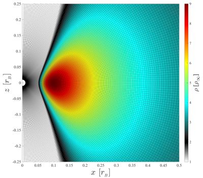
Figure 1: The two-dimensional density distribution of the initial equilibrium torus overlaided with the grid structure of our simulations. The maximum density is located at $0.1\,r_{{}_{\rm B}}$. In $\theta$-direction, we set $N_{\theta}=200$ equally spaced grids while in the $r$-direction, logarithmic grid has be adopted which has the advantage of preserving the cell aspect ratio at any distance from the origin. The values of $N_{r}$ and $r_{\rm max}$ are evaluating so that we have squared cells in each direction.

$$\log_{{}_{10}}\left(\frac{r_{\rm max}}{r_{\rm min}}\right)=N_{r}\log_{{}_{10}}\left(\frac{2+\Delta\theta}{2-\Delta\theta}\right).$$ (11)

The above formula gives us $r_{\rm max}=30\,r_{{}_{\rm B}}$. In addition, preserving the cell aspect ratio at any distance is necessary for correctly calculating flux at the left and right faces of each individual cell used in finite volume method. Using radial logarithmic grid can also guarantee a good resolution near the inner region of our computational domain where the viscosity becomes important. For the reconstruction of the characteristic variables within a cell, we adopted the third-order piecewise parabolic method (PPM; Colella & Woodward 1984) which has been implemented in PLUTO code. The time step $\Delta t$ is computed using third-order total variation diminishing (TVD) Runge Kutta method (RK3) with the CFL number 0.4. In addition, we adopt Harten, Lax, Van Leer approximate Riemann solver that restores with the middle contact discontinuity (HLLC). Therefore, compared to Inayoshi et al. 2018, 2019, we have high-order of accuracy in both space and time. Moreover, as we explained in the previous section, we run some models in the presence of thermal conduction.

2.3 Initial and boundary conditions

As initial condition, we assume a rotating equilibrium torus $(v_{r}=v_{\theta}=0)$ with a constant specific angular momentum of $\ell$, embedded in a non-rotating, low-density medium. Starting from the momentum equation and considering polytropic equation of state, $p=A\,\rho^{\gamma}$, where $A$ is a constant, the density distribution of the torus will be determined as,

$$\frac{\rho_{t}}{\rho_{\infty}}=\left[1+\left(\gamma-1\right)\frac{GM}{c_{\rm s,\infty}^{2}r}-\frac{\gamma-1}{2}\frac{\ell^{2}}{c_{\rm s,\infty}^{2}\varpi^{2}}\right]^{1/(\gamma-1)},$$ (12)

where $\varpi=r\sin\theta$ is the cylindrical radius and the value of adiabatic index is set to $\gamma=5/3$. When the right-hand side of the above equation is positive, the density profile is valid. For the region near the rotation axis the right hand-side of Equation (12) becomes negative and the ambient medium density is chosen to be $\rho_{a}=10^{-4}\rho_{\rm crit}$, which is too small to affect our results. The maximum value of the density, $\rho_{\rm crit}$, is located at centrifugal radius $r_{\rm{}_{C}}$. The initial density distribution is plotted in Figure 1. By defining the constant specific angular momentum as $\ell=\sqrt{\beta}\,r_{\rm{}_{B}}c_{\rm s,\infty}$, where $\beta=r_{\rm{}_{C}}/r_{\rm{}_{B}}$, the maximum density is evaluated as,

$$\rho_{\rm crit}=\rho_{\infty}\left[1+\frac{\gamma-1}{2\beta}\right]^{1/(\gamma-1)}.$$ (13)

Here we assume $\beta<1$ leading to the case of $r_{\rm s}\ll r_{\rm{}_{C}}<r_{\rm{}_{B}}$. We set $\beta=0.1\,r_{\rm{}_{B}}$ throughout this paper. Note that in the absence of viscosity and radiative cooling, the material with $r_{\rm{}_{C}}>r_{\rm{}_{B}}$ cannot accrete and forms a thick torus near the equator. This thick torus and its formation have been a subject of numerous studies (see e.g., Papaloizou & Pringle 1984; Proga & Begelman 2003a, b). Since the centrifugal radius is very large compared to the Schwarzschild radius, the inflowing hot gas always fall to a rotating disk before reaching the back hole, due to the outward transport of angular momentum mechanism (Lynden-Bell & Pringle 1974; Pringle 1981). To avoid numerical error, we adopt the density and temperature floor as $\rho_{\rm floor}=10^{-4}\rho_{\rm crit}$ and $T_{\rm floor}=10^{4}\,\rm{K}$ respectively, which is far beyond having any effect to our simulation results.

For the boundary conditions, we adopt the outflow boundary condition at the inner and outer radial boundaries (e.g. Stone & Norman 1992). We also impose $v_{r}\leq 0$ at the inner boundary which means that inflow of the gas from ghost cells is prohibited. We use the axisymmetric boundary conditions at both poles $(\theta=\epsilon,\pi-\epsilon)$.

3 Results

Table 1: Summary of Models

Model	Thermal Conduction	$\alpha_{\rm c}$	$\dot{M}_{\rm acc}$
A	NO	—	$4.40\times 10^{-3}$
B	YES	0.2	$1.51\times 10^{-2}$
C	YES	0.5	$2.69\times 10^{-2}$

Note. — The avarage mass accretion rates are in the units of Bondi accretion rate, $\dot{M}_{\rm{}_{B}}$, evaluated by Equation 14. The mass accretion rates are time-averged over $2\leq t/t_{\rm orb}\leq 4$.

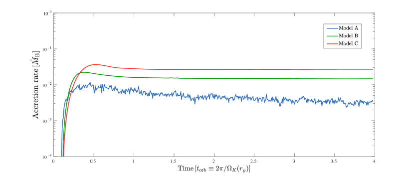
Figure 2: Time evolution of the net accretion rate (in units of the Bondi rate) at $r_{\rm in}=10^{-2}r_{\rm{}_{B}}$ for Model A (blue), Model B (green) and Model C (red). Here we set the viscosity parameter to be $\alpha_{{}_{0}}=0.01$.

3.1 Parameter choices and models

Before we discuss our simulation results, we introduce the physical units and the numerical models that characterize our hot accretion flow simulations at large radii. At the initial state, we set the density and temperature of the gas at infinity to $\rho_{\infty}=10^{-22}\,\rm{g\,cm^{-3}}$ and $T_{\infty}=10^{7}\,\rm{K}$, respectively. This temperature is equivalent to the sound speed of $c_{\rm s,\infty}=\sqrt{\gamma k_{\rm B}T_{\infty}/(\mu m_{\rm p})}=4.7\times 10^{7}\rm{cm\ s^{-1}}$ with $\mu=0.62$. In our units, we scale all the spatial scales with $r_{\rm{}_{B}}$, velocities with $c_{\rm s,\infty}$, and density with the density at infinity $\rho_{\infty}$. Therefore, units of time, pressure $p$, and the kinematic viscosity coefficient $\nu$ will be $r_{\rm{}_{B}}/c_{\rm s,\infty}$, $\rho_{\infty}c_{\rm s,\infty}^{2}$ and $c_{\rm s,\infty}r_{\rm{}_{B}}$, respectively. Unless stated otherwise, time-scales are evaluated in terms of the orbital time scale of a test particle at Bondi radius which is given by $t_{\rm orb}=2\pi/\Omega_{\rm{}_{K}}(r_{\rm{}_{B}})$. Bondi accretion rate is well defined and standard reference of the accretion rate from the Bondi radius which can be written as

$$\dot{M}_{\rm B}=4\pi\lambda(\gamma)\rho_{\infty}\frac{G^{2}M^{2}}{c_{\rm s,\infty}^{3}},$$ (14)

where $\lambda(\gamma)=1/4$ for $\gamma=5/3$. We should note that the accretion parameter $\lambda$ can strongly depend on the galaxy potential at very large distances from the central BH, and therefore the Bondi accretion rate will be much larger than the expected for assigned density and temperature at infinity (e.g., see Ciotti & Pellegrini 2017, 2018; Mancino et al. 2022). We normalize mass accretion rates with Bondi accretion rate throughout this paper. The viscous parameter is set to $\alpha_{{}_{0}}=0.01$.

In this study, we perform hydrodynamical simulations of hot accretion flow at large radii. In all simulations presented here, the viscosity is modeled base on Equations (7)-(9) and we ignored the radiative losses. In model A we simulate hot accretion flow without thermal conduction and investigate the existence of wind. Moreover, we carry out two models, i.e., models B and C, to study the effects of thermal conduction on wind. The conductivity coefficient of model B and C is considered as $\alpha_{c}=0.2$ and $0.5$, respectively. Details of the simulation models are tabulated in Table 1. The last column of Table 1 represents the time-averaged mass accretion rate through the inner boundary in the units of Bondi accretion rate.

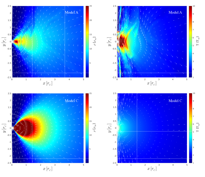
Figure 3: Snapshots of contours of gas density (left-hand column) and temperature (right-hand column) correspond to models A and C, respectively. The elapsed time is set to $t=4t_{\rm orb}$. The densities and temperatures are over-plotted with the poloidal velocity $\bm{v}_{\rm p}=v_{r}\hat{\bm{r}}+v_{\theta}\hat{\bm{\theta}}$. Arrows on the density profiles show only the direction of velocity $(\bm{v}_{\rm p}/\left|\bm{v}_{\rm p}\right|)$, while the arrows on the temperature profiles indicate both the magnitude and direction of the poloidal velocity. The dotted white curves in the left panels show the location of the centrifugal radius $r_{\rm{}_{C}}=0.1r_{\rm{}_{B}}$.

3.2 Mass inflow rate

Following Stone et al. 1999, the mass inflow and outflow rates, $\dot{M}_{\rm in}$ and $\dot{M}_{\rm out}$, will be defined as,

$$\dot{M}_{\rm in}=2\pi r^{2}\int_{0}^{\pi}\rho\,\mathrm{min}(v_{r},0)\sin\theta d\theta,$$ (15)

$$\dot{M}_{\rm out}=2\pi r^{2}\int_{0}^{\pi}\rho\,\mathrm{max}(v_{r},0)\sin\theta d\theta.$$ (16)

The total mass outflow rate calculated by equation (16) is includes real outflow and outward moving portion of turbulent eddies, since this consists of all of the fluid with positive velocity. In the following, we use wind to denote real outflow.

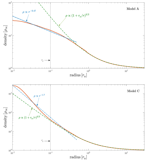
Figure 4: Radial profile of the gas density along the equatorial plane for Models A (top panel) and C (bottom panel). The density profiles are time-avarge over $2\leq t/t_{\rm orb}\leq 4$ and angle-average over $80^{\circ}\leq\theta\leq 110^{\circ}$. The dotted lines show the location of circularization radius, $r_{\rm{}_{C}}=0.1r_{\rm{}_{B}}$. At the region of $r\geq 2r_{\rm{}_{C}}$, the density profiles of both models approximately follow $\rho\propto(1+r_{\rm{}_{B}}/r)^{3/2}$, (green dashed lines). In the inner region, the radial density profile of model A follows $\rho\propto r^{-0.47}$, while for model C, in the presence of thermal conduction, it follows $\rho\propto r^{-1.7}$ (blue dash-dotted lines).

The net mass accretion rate can be written as,

$$\dot{M}_{\rm acc}=2\pi r^{2}\int_{0}^{\pi}\rho\,v_{r}\sin\theta d\theta,$$ (17)

which is $\dot{M}_{\rm acc}=\dot{M}_{\rm in}+\dot{M}_{\rm out}$. Figure 2 shows the time evolution of the angle-integrated mass accretion rate $\dot{M}_{\rm acc}$ at $r=0.01r_{\rm{}_{B}}$ (i.e., the inner boundary) for Model A (blue), Model B (green) and Model C (red). We normalize the simulation time by the orbital time-scale $t_{\rm orb}$ at the Bondi radius and the mass accretion rate by Bondi accretion rate $\dot{M}_{\rm{}_{B}}$. Since the angular momentum of the gas is set equal to the Keplerian angular momentum at $r_{\rm{}_{C}}=0.1r_{\rm{}_{B}}$, it is natural that the gas at the outer part tends to accumulate around this region because of the black hole gravity. Moreover, due to the form of viscosity (see equation (9)), this process starts to work at the region of $r<r_{\rm{}_{C}}$, so that the angular momentum of the gas can be transported outward, which drives inflow gas motion in a quasi-steady fashion.

Our runs have been evolved around $4$ orbits at Bondi radius. From this figure we can see that for all models, the mass accretion rate rapidly increases until $t\leq 0.5t_{\rm orb}$. Then the quasi-steady accretion phase starts at the range of $0.5\,t_{\rm orb}<t\leq 4\,t_{\rm orb}$ and all the physical quantities become nearly constant. The fourth column of Table 1 also shows the corresponding time-averaged mass accretion rate over $0.5\,t_{\rm orb}<t\leq 4\,t_{\rm orb}$. For Model A, the accretion rate has fluctuations at $t>0.5\,t_{\rm orb}$ and oscillates with very small amplitude around its mean value $\dot{m}=\dot{M}_{\rm acc}/\dot{M}_{\rm{}_{B}}\simeq 4.40\times 10^{-3}$. The behavior of the accretion rates in model B and C, where the thermal conduction is presented, is similar and greater than model A. In fact, the time-averaged values of Model B and C in the quasi steady-state case are $\dot{m}=1.51\times 10^{-2}$ and $\dot{m}=2.69\times 10^{-2}$ respectively (see the column 4 of Table 1). This result shows that thermal conduction increases the mass accretion rate by one order of magnitude from the case without conduction. From Figure 2, it appears that model A (model with no thermal conditions) is noisier than models B and C where the thermal conditions is presented. This is due to the rapid time variation of poloidal velocity and gas density in model A than models B and C. The main reason is as follows: in model A, where the thermal condition is not included, the accretion flow is quite turbulent and convective motions result in the turbulent nature of the accretion flow. On the other hand, for models with thermal conduction, model B and C, the accretion flow becomes quite laminar which means the convective motion is not important and significantly supressed.

3.3 Our fiducial models

We choose model A (without thermal conduction) and model C (with thermal conduction) as our fiducial models in this paper. Figure 3 shows the snapshot of the gas density (left-hand column) and temperature (right-hand column) corresponding to the models A and C. The elapsed time is set to $t=4t_{\rm orb}$. The densities and temperatures are over-plotted with the poloidal velocity $\bm{v}_{\rm p}=v_{r}\hat{\bm{r}}+v_{\theta}\hat{\bm{\theta}}$. Arrows on the density profiles show only the direction of velocity $(\bm{v}_{\rm p}/\left|\bm{v}_{\rm p}\right|)$, while the arrows on the temperature profiles indicate both the magnitude and direction of the poloidal velocity. The dotted white curves in the left panels show the location of the centrifugal radius $r_{\rm{}_{C}}=0.1r_{\rm{}_{B}}$. From the density profile of both models, it is clear that the maximum density region is located inside $r_{\rm min}<r<2r_{\rm{}_{C}}$. The reason is that the angular momentum $\ell$ begins to be transported outwards due to definition of the viscosity parameter in our models. Equation (9) shows that viscosity highly depends on the threshold of the density, $\rho_{\rm crit}$, above which the viscosity will be turned on. The density around the midplane has increased in model C, with thermal conduction. To know how thermal conduction affects the temperature of the flow, we should compare the right panels of Figure 3. In both top and bottom right panels of this figure, the gas temperature is increasing toward the centre due to the compression heating of the black hole gravity and dissipation heating produced by viscosity. It is also clear that in the model without thermal conduction, the temperature in the dense core of the accretion flow becomes higher than $T>10^{8}\,K$ while the maximum temperature in model C with thermal conduction is about $T\sim 5-6\times 10^{7}$. Temperature decrease in model C will result in the density increase. This is because when the temperature increase in the vertical direction, the pressure will support the disk. Consequently, if the temperature decreases, the density will increase to sustain the fix pressure. In model C, the temperature is also distributed homogeneously around the central black hole.

To show that why the net mass accretion rate increases in models with thermal conduction, both the density and temperature profiles are overplotted with the direction and magnitude of the poloidal velocity. From the right column of Figure 3 we see that in model C most fraction of the gas is inflowing from inside the Bondi radius and is directed towards the central black hole. On the other hand, for model A we observe strong wind (long arrows) at the disk surface and also inflow and outflow motions in circulation at this inner region. From the arrows in the left column we can see that in both models, very close to the rotation axis, the gas is inflowing towards the central black hole. Moreover, in model A the mirror symmetry of the hot accretion flow cross the midplane is broken. In model C, where the thermal conduction is presented, the accretion disk is almost symmetric above and below the equatorial plane.

The density profiles as well as magnitude of the poloidal velocity clearly show the reason why the mass accretion rate in the presence of thermal conduction has increased one order of magnitude compared to the case without conduction (see, Equation (17) for more details about the dependency of net accretion rate to the density and radial velocity).

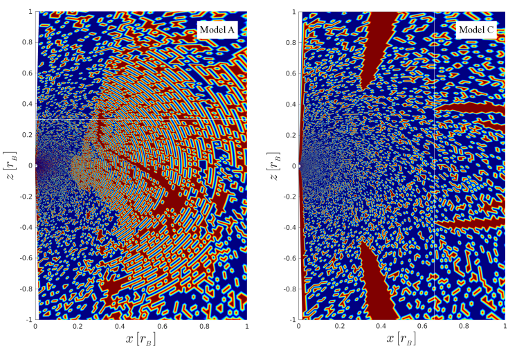
Figure 5: Convective stability analysis of models A (left panel) and C (right panel). The results are obtained according to Equations (18) and (19) based on simulation data time-averaged over $2\leq t/t_{\rm orb}\leq 4$. The red color denotes unstable regions.

Figure 4 shows the radial profile of gas density in the equatorial plane for model A (top panel) and C (bottom panel) in order to understand the properties of hot accretion flow with/without thermal conduction. The density profiles are time-averged over $2\leq t/t_{\rm orb}\leq 4$, and angle-average over $80^{\circ}\leq\theta\leq 110^{\circ}$. The dotted lines show the location of circularization radius, $r_{\rm{}_{C}}=0.1r_{\rm{}_{B}}$. From this figure we can see that at the outer region accretion flow, $r\geq 2r_{\rm{}_{C}}$, the density profiles of both models perfectly follow $\rho\propto(1+r_{\rm{}_{B}}/r)^{3/2}$, (see green dashed lines). For the inner region, the radial density profile of model A fit well with $\rho\propto r^{-0.47}$, while for model C, in the presence of thermal conduction, it follows $\rho\propto r^{-1.7}$ (see blue dash-dotted lines). This implies that when the thermal conduction is not considered in the flow, the profile of the density has a smoother trend at the inner region as shown in this figure. We emphasize here that, based on the radial profile of the density at the equatorial plane, Inayoshi et al. 2018 argued that this profile is the consist of two components: (1) a rotational equilibrium solution at the outer region ($r>2r_{\rm{}_{C}}$) which follows $\rho\propto(1+r_{\rm{}_{B}}/r)^{3/2}$, and (2) a convection dominated regions at the inner region ($r<2r_{\rm{}_{C}}$) follows $\rho\propto r^{-1/2}$. More precisely, based on the density profile, they argued that decrease of mass accretion rate inward is because of convective motion. Therefore they concluded that the inner region agrees well with the CDAF solution and there is no wind. In the following subsection we investigate the convective stability of the hot accretion flow with/without thermal conduction.

3.4 Convective Stability

Numerical HD simulations of hot accretion flow have been found that the flows are convectively unstable (see i.e., Stone et al. 1999; Igumenshchev & Abramowicz 1999, 2000; Yuan & Bu 2010; Bu et al. 2016a). This also have been suggested by one-dimensional self-similar solutions of Narayan & Yi 1994. The main physical reason is as follow, due to the viscous dissipative heating and negligible radiative loss, the entropy of the hot accretion flow increases inward. In this subsection we investigate the convective stability of hot accretion flows at large radii based on our numerical simulation results of models A and C. To treat the convective stability of the flow, the well-known Solberg-Høiland criterions in cylindrical coordinates $(\varpi,\phi,z)$ will be adopted (e.g., Tassoul 2000). If the hot accretion is convectively stable, both of the two following criteria shall be positive:

$$-\frac{1}{\gamma\rho}\bm{\nabla}p\cdot\bm{\nabla}s+\frac{1}{\varpi^{3}}\frac{\partial\ell^{2}}{\partial\varpi}\geq 0,$$ (18)

$$-\frac{\partial p}{\partial z}\left(\frac{\partial\ell^{2}}{\partial\varpi}\frac{\partial s}{\partial z}-\frac{\partial\ell^{2}}{\partial z}\frac{\partial s}{\partial\varpi}\right)\geq 0,$$ (19)

where $s=\ln(p/\rho^{\gamma})$ is the entropy. We adopt the following transformations to find the angular dependency of two Solberg-Høiland criteria in spherical coordinates,

$$\frac{\partial}{\partial\varpi}=\sin\theta\frac{\partial}{\partial r}+\frac{\cos\theta}{r}\frac{\partial}{\partial\theta},$$ (20)

$$\frac{\partial}{\partial z}=\cos\theta\frac{\partial}{\partial r}-\frac{\sin\theta}{r}\frac{\partial}{\partial\theta}.$$ (21)

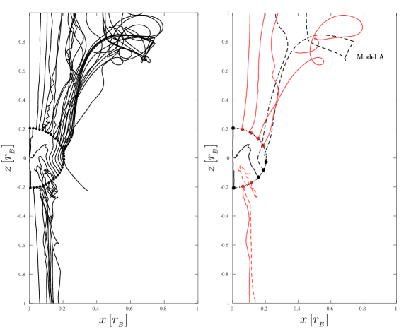
Figure 6: Various types of trajectory of test particles for model A. The dots located at $r=0.2r_{\rm{}_{B}}$ are starting points of the particles. In the left panel we select 34 particles in diferent $\theta$ angles and significant winds are clearly present. In the right panel, the red lines denote outflow, while black ones are for inflow. See subsection 3.5 for details.

The convective stability analysis of models A and C are shown in Figure 5. The results are obtained according to Equations (18) and (19) based on simulation data time-averaged over $2\leq t/t_{\rm orb}\leq 4$. The red color denotes unstable regions. The result indicates that in both models the convectively unstable regions exist. The physical reason is the same as we explained before: during the accretion process, in the absence of radiative cooling, due to the viscous dissipated heating the entropy of the gas increases inward. Moreover, although in both models convectively unstable regions exist, for model C when the thermal conduction is included (right panel), the stable regions are larger and the convection motions are suppressed.

Previous works such as Yuan et al. 2012a showed that strong winds are produced in HD hot accretion flows around black holes. They found that the driving force for wind production in such a system is mainly buoyant force associated with the convection instability. In the next subsection, following Yuan et al. 2015, we use trajectory particle method to study whether winds exist at such large radii.

3.5 Trajectory Method

In the turbulent flow the existing turbulent eddies move outwards and consequently have positive radial velocities. In principle, they are not real outflow and are only portion of turbulent motions. On the other hand we have real outflow, where the flow go outward and escape to the large radii. The real outflow is called wind. One technique that we adopt to characterize and identify wind based on our mesh-based simulations is ”trajectory test particles” which are passively advected with the flow, and thereby track its Lagrangian evolution, allowing the thermodynamical history of individual fluid elements to be recorded. This technique is named La‌grangian particle tracking method and has been used in several different astrophysical simulations. We utilize the trajectory method to distinguish between turbulent outflow and real outflow (see, Yuan et al. 2015). The difference between outflow and real outflow is that the outflow might be turbulent outflow which particles rejoin the flow after flowing outward. The real outflow is considered for the particles that go outward and escape the outer boundary of the simulation domain. As we mentioned, trajectory is related to the Lagrangian description of the fluid, and obtained by following the motion of fluid elements at consecutive times. The superiority of the trajectory method to the streamlines is that it is used for the turbulent motion such as accretion flow. The trajectory is analogous to the streamline just when the flow has steady motion.

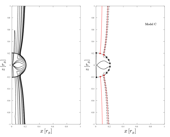
Figure 7: Same as figure 6, but for model C.

As it is stated before, Inayoshi et al. 2018 performed similar simulations in the absence of thermal conduction and based on the radial profile of density, they argued that there exists no outflow. More precisely, they claimed that convective motions results in inward decrease of mass accretion rate. Here, using trajectory method, we will consider a set of virtual test particles in the simulation domain at different radii to extensively study the wind. Following Yuan et al. 2015, We use “outflow” to describe any flow with a positive radial velocity i.e., $v_{r}>0$, flowing outward. This can be both “turbulent outflow” and “real outflow”. The main difference between them is that in the turbulent case the test particle will return and join the accretion flow after flowing outward for some distance. On the other hand, in the case of real outflow the test particle continues to flow outward and eventually escapes the outer boundary of our computational domain.

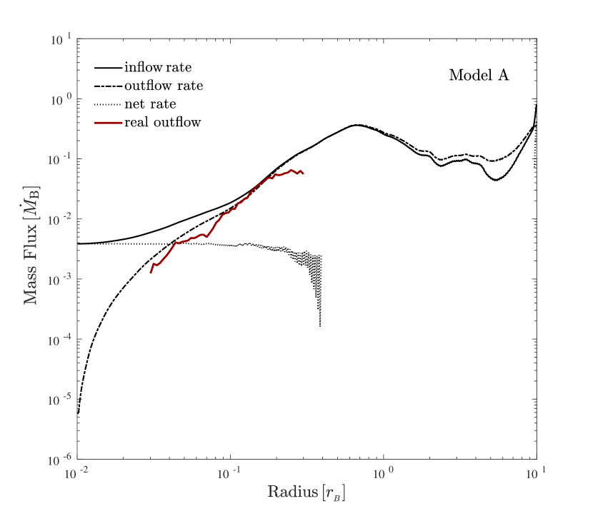
Figure 8: Radial profile of the time-averaged mass inflow rate (solid black line), outflow rate (dash-dotted line), net rate (dotted line), and real outflow (solid red line) for models A (left panel) and C (right panel). The results are time-averaged over $2t_{\rm orb}\leq t\leq 4t_{\rm orb}$. We do the trajectory analysis inside $0.3r_{\rm{}_{B}}$, since the quasi-steady state solutions achieved in this region.

By adopting the trajectory method, we can discriminate which particles are real outflow and which ones are turbulent motions. The left panel of Figure 6 shows the trajectory of 34 test particles staring from $r=0.2r_{\rm{}_{B}}$ in model A (without thermal conduction). From this figure we can clearly see the real wind trajectories, i.e., the particles that extend from $r=0.2r_{\rm{}_{B}}$ to the large radii above the Bondi radius would never cross $r=0.2r_{\rm{}_{B}}$ twice. Note here that distinguishing the types of characteristic particle trajectories is crucial for calculating the mass fluxes of the real outflow correctly. Therefore, in the right panel of Figure 6 we distinguish inflow and outflow with black and red lines, respectively. Here, the red solid lines show the real outflow, where the particles keep moving outward and never cross the radius $r=0.2r_{\rm{}_{B}}$ again. Moreover the red dashed line represents the turbulent outflow, where the particle first move outward but will return and cross the radius $r=0.2r_{\rm{}_{B}}$ during its motion, and eventually move outward. In this figure, the black solid lines represent real inflow while the black dashed lines are turbulent inflow.

Figure 7 is the same as figure 6, but for model C in the presence of thermal conduction. Based on this figure we can see that in the region around equatorial plane, the particles are inflow particles which move toward the central black hole, while at the high latitudes we have more outflow motions. Compared to the model A, in model C, the trajectory particles have a symmetrical traces above and below the equator. In addition, in both models the particles very close to the rotation axis move towards the centre as inflow particles.

After obtaining the trajectories, we calculate the mass fluxes in the last part of this section. Figure 8 shows the radial profile of the time-averaged (from $t=2$ to 4 orbits) mass inflow rate (solid black line), outflow rate (dash-dotted line), the net rate (dotted line), calculated from Equations (15)-(17). The red lines denote the mass flux of the real outflow evaluated by trajectory method. We do the trajectory analysis inside $0.3r_{\rm{}_{B}}$, since the quasi-steady state solutions are achieved in this region. This figure clearly shows that for both models, the wind exist inside the Bondi radius. The inflow and outflow rates decrease toward the central black hole. The inflow profile in model C is more flattened with respect to model A. More specifically, in the region $0.01<r<0.1$ of model C, the prominence of the inflow over the outflow is due to the existence of thermal conduction. The reason is that conduction can take away the release gravitational energy of the accretion flow. In this case it is not necessary to have a strong wind to take a way the release gravitational energy for the accretion process to occur. In model A the mass outflow rate increases from larger radii, and reaches to maximum amount at $0.8\,r_{\rm{}_{B}}$ compared with model C. Even more, in model A the real outflow starts to begin at smaller radius around $0.03\,r_{\rm{}_{B}}$ while it starts around $0.04r_{\rm{}_{B}}$ in model C.

In addition, to quantitatively investigate the wind, we calculated the ratio of mass flux of winds to the total outflow rate at $r=0.2r_{\rm{}_{B}}$. This ratio for model A and C is $84\%$ and $78\%$ respectively. Our quantitative calculation of the ratio of mass flux of winds to the total outflow rate based on trajectory method clearly confirms that the wind exists in hot accretion flow and can reach to large radii. Although in previous study of Inayoshi et al. 2018 they did not find wind in their solution, our results show that very effective wind can be produced inside the Bondi radius. Therefore, we conclude that the decrease of mass accretion rate inward is due to the wind rather than the convection at such large radii.

4 Summary

Numerical HD and MHD simulations of hot accretion flow around black hole show that strong wind must be present in such a system. For instance, Yuan et al. 2015 found that the mass flux of wind follows $\dot{M}_{\rm wind}=\dot{M}_{\rm{}_{BH}}(r/20r_{\rm s})$. Subsequently, the main question is how far the wind can be produced? In order to answer this question, we study hot accretion flow on a SMBH with two-dimensional hydrodynamical simulations. The accretion flow is considered to be axisymmetric. We only take into account the gravity of the central black hole and neglect the nuclear stars gravity. Moreover, the radiative losses and relevant AGN feedback are not considered in this study. In our hydrodynamical simulations, we adopt $\alpha$ prescription of viscosity to mimic the effect of the magnetic stress. In some of our models, we include thermal conduction and compare the results with the case without conduction. The runs have been evolved around 4 orbits at Bondi radius. For all of our models, the mass accretion rate from the inner boundary of our computational domain becomes almost constant at the range of $0.5t_{\rm orb}<t\leq 4t_{\rm orb}$ which indicates that the flow reaches to the steady state. For our model without thermal conduction, the mass accretion rate has some oscillation at $t>0.5t_{\rm orb}$ with very small amplitude around its mean value, while the accretion rates in models with thermal conduction are almost constant and greater than model A (a model with thermal conduction). Furthermore, the density around the midplane has increased in models incorporating thermal conduction and a thick and hot accretion flow forms.

We investigate the convective stability of the hot accretion flow with/without thermal conduction at large radii based on our numerical simulation results. Our results show that for both models the disk is convectively unstable. Although both models are convectively unstable, thermal conduction could slightly decrease the instability (see Figure 5). In previous simulation of Inayoshi et al. 2018, they found a global steady accretion solution with two distinguished regimes: (1) the outer rotational equilibrium region around Bondi radius follows the density profile of $\rho\propto(1+r_{\rm{}_{B}}/r)^{3/2}$ and (2) the inner solution where the geometrically thick torus follows $\rho\propto r^{-1/2}$. Based upon the density profile of inner part, they argued that the physical properties of this region are consistent with the convection-dominated accretion flows (CDAFs) rather than Adiabatic Inflow-Outflow Solutions (ADIOS). In order to understand the properties of hot accretion flow with/without thermal conduction, the density profiles at the equatorial plane have been checked. We found that at the outer region of accretion flow, $r\geq 2r_{\rm{}_{C}}$, the density profiles of all models perfectly follow $\rho\propto(1+r_{\rm{}_{B}}/r)^{3/2}$. In the inner region, the radial density profile of model without thermal conduction fits well with $\rho\propto r^{-0.47}$, while for model in the presence of thermal conduction, it follows $\rho\propto r^{-1.7}$. This implied that when the thermal conduction is not considered in the flow, the profile of the density has a smoother trend at the inner region

To show the existence of outflow based on a direct way, we use a trajectory approach in this work. We set 34 trajectory test particles staring from $r=0.2r_{\rm{}_{B}}$ and our results clearly show the real wind trajectories. In principle, there exist particles that extend from starting points to the large radii above the Bondi radius and never cross $r=0.2r_{\rm{}_{B}}$ twice. After obtaining the trajectories, we also calculate the mass fluxes of inflow, outflow, as well as real wind. In addition, to quantitatively investigate the wind, we calculated the ratio of mass flux of winds to the total outflow rate at $r=0.2r_{\rm{}_{B}}$. Our results show that about $80\%$ of the total mass flux of outflow is real wind at this radius. Our quantitative calculation based on the mass fluxes and trajectory method can clearly confirm that the real wind exist in hot accretion flow and can reaches to large radii. Although in previous study of Inayoshi et al. 2018 they found no outflow, here the key difference between our work and their work is we found that a very effective wind can be produced inside the Bondi radius. Hence, we conclude that the inward decrease of the mass accretion rate will be due to the wind rather than the convection at such large radii.

Bu et al. 2016a, b also studied the accretion flow around Bondi radius. They find that after including the gravity of nuclear stars, the physics can be totally changed. Specifically, they find that in the presence of nuclear star gravity, the winds can not be produced locally. They also did some test and find that when the neclear star gravity is excluded, the winds can be generated locally around Bondi radius. Therefore, the result that the presence of winds near Bondi radius found in the present paper is not conflict with that of Bu et al. 2016a, b.

Based on the above argument, for the hot accretion flow around the Bondi radius in a real galaxy, whether winds can be produced locally around Bondi radius depends on the presence or strength of nuclear star gravity. Around the Bondi radius, If the black hole gravity is significantly dominate the nuclear star gravity, we will expect strong winds generated around Bondi radius. However, if the nuclear star gravity dominates, no winds can be expected around Bondi radius.

There are several caveats in our study that will be improved in our future simulations. The first one is that we only consider the HD equations of hot accretion flow for our simulations. In a real accretion flow, angular momentum is transferred by Maxwell stress associated with MHD turbulence driven by MRI. Moreover, the magnetic field is one of the driving mechanisms for wind production. With this aim, we will preform the MHD simulations of the accretion flow at large radii. In our future work we will mainly focus on different magnetic field configurations on the structure of the hot accretion flow and compare the results with the HD simulations. A further simplification here is that we only considered the gravity of the central black hole. Our estimation shows that in this range of radii the nuclear stars gravity might be taking into account. Moreover, one-temperature fluid equations are considered here. In terms of hot accretion model, the ions are expected to be much hotter than the electrons (see Rees et al. 1982; Yuan & Narayan 2014). Thus, two different energy equations for electrons and ions should be solved.

References

- Antonucci (2012) Antonucci R., 2012, A&AT, 27, 557
- Balbus & Hawley (1998) Balbus, S. A., & Hawley, J. F. 1998, \rmp, 70, 1
- Begelman (2012) Begelman, M. C. 2012, MNRAS, 420, 2912
- Belloni (2010) Belloni, Tomaso M. 2010, The Jet Paradigm. Springer, Berlin, Heidelberg, 53-84
- Blandford & Begelman (1999) Blandford, R. D., & Begelman, M. 1999, MNRAS, 303, 1
- Blandford & Begelman (2004) Blandford, R. D., & Begelman, M. 2004, MNRAS, 349, 68
- Bondi (1952) Bondi H., 1952, MNRAS, 112, 195
- Bu et al. (2016) Bu, D.-F., Wu, M.-C., and Yuan, Y.-F. , 2016, MNRAS, 459, 746
- Bu et al. (2016a) Bu, D.-F., Yuan, F., Gan, Z.-M., & Yang, X.-H. 2016a, ApJ, 818, 83
- Bu et al. (2016b) Bu, D.-F., Yuan, F., Gan, Z.-M., & Yang, X.-H. 2016b, ApJ, 823, 90
- Ciotti & Pellegrini (2018) Ciotti L., Pellegrini S., 2018, ApJ, 868, 91
- Ciotti & Pellegrini (2017) Ciotti L., Pellegrini S., 2017, ApJ, 848, 29
- Colella & Woodward (1984) Colella P., & Woodward P. R., 1984, JCoPh, 54, 174
- Gu (2015) Gu, W. M. 2015, ApJ, 799, 71
- Johnson & Quataert (2007) Johnson, B. M., & Quataert, E. 2007, ApJ, 660, 1273
- Ho (2008) Ho, Luis C. 2008 Annu. Rev. Astron. Astrophys. 46, 475-539
- Igumenshchev & Abramowicz (1999) Igumenshchev I. V., Abramowicz M. A., 1999, MNRAS, 303, 309
- Igumenshchev & Abramowicz (2000) Igumenshchev I. V., Abramowicz M. A., 2000, ApJS, 130, 463
- Inayoshi et al. (2018) Inayoshi, K., Ostriker, J. P., Haiman, Z., & Kuiper, R. 2018, MNRAS, 476, 1412
- Inayoshi et al. (2019) Inayoshi, K., Ichikawa, K., Ostriker, J. P., & Kuiper, R. 2019, MNRAS, 486, 5377
- Li et al. (2013) Li, J., Ostriker, J., & Sunyaev, R. 2013, ApJ, 767, 105
- Lynden-Bell & Pringle (1974) Lynden-Bell D., Pringle J. E., 1974, MNRAS, 168, 603
- Mignone et al. (2007) Mignone A., Bodo G., Massaglia S., Matsakos T., Tesileanu O., Zanni C., Ferrari A., 2007, ApJS, 170, 228
- Narayan et al. (2000) Narayan, R., Igumenshchev, I. V., & Abramowicz, M. A. 2000, ApJ, 539, 798
- Narayan & McClintock (2008) Narayan R, McClintock J. E., 2008, New Astron. Rev., 51:733–511
- Narayan et al. (2012) Narayan, R., Sadowski, A., Penna, R. F., & Kulkarni, A. K. 2012, MNRAS, 426, 3241
- Narayan & Yi (1994) Narayan R., Yi I., 1994, ApJ, 428, L13
- Mancino et al. (2022) Mancino, A, Ciotti L., Pellegrini S., 2022, MNRAS, 512, 2474
- Ostriker et al. (2010) Ostriker, J. P., Choi, E., Ciotti, L., Novak, G. S., & Proga, D. 2010, ApJ, 722, 642
- Papaloizou & Pringle (1984) Papaloizou J. C. B., Pringle J. E., 1984, MNRAS, 208, 721
- Pringle (1981) Pringle J. E., 1981, ARA&A, 19, 137
- Proga & Begelman (2003a) Proga D., Begelman M. C., 2003a, ApJ, 582, 69
- Proga & Begelman (2003b) Proga D., Begelman M. C., 2003b, ApJ, 592, 767
- Quataert (2008) Quataert, E. 2008, ApJ, 673, 758
- Rees et al. (1982) Rees, M. J., Phinney, E. S., Begelman, M. C., & Blandford, R. D. 1982, Natur, 295, 17
- Shakura & Sunyaev (1973) Shakura, N. I., & Sunyaev, R. A. 1973, A&A, 24, 337
- Sharma et al. (2008) Sharma, P., Quataert, E., Stone, J. M. 2008, MNRAS, 389, 1815
- Stone & Norman (1992) Stone J. M., Norman M. L., 1992, ApJS, 80, 753
- Stone & Pringle (2001) Stone, J. M., & Pringle, J. E. 2001, MNRAS, 322, 461
- Stone et al. (1999) Stone, J. M., Pringle, J. E., & Begelman, M. C. 1999, MNRAS, 310, 1002
- Tassoul (2000) Tassoul, J. L. 2000, Stellar Rotation (Cambridge: Cambridge Univ. Press)
- Wang et al. (2013) Wang, Q. D., Nowak, M. A., Markoff, S. B., et al. 2013, Sci, 341, 981
- Yuan & Bu (2010) Yuan F., Bu D., 2010, MNRAS, 408, 1051
- Yuan et al. (2012a) Yuan, F., Bu, D., & Wu, M. 2012a, ApJ, 761, 130
- Yuan et al. (2015) Yuan, F., Gan, Z. M., Narayan, R., et al. 2015, ApJ, 804, 101
- Yuan & Narayan (2014) Yuan, F., & Narayan, R. 2014, ARA&A, 52, 529
- Yuan et al. (2012b) Yuan, F., Wu, M., & Bu, D. 2012b, ApJ, 761, 129