Dalek II - Emulator framework with probabilistic inference

Probabilistic Dalek - Emulator framework with probabilistic prediction for supernova tomography

Abstract

Supernova spectral time series can be used to reconstruct a spatially resolved explosion model known as supernova tomography. In addition to an observed spectral time series, a supernova tomography requires a radiative transfer model to perform the inverse problem with uncertainty quantification for a reconstruction. The smallest parametrizations of supernova tomography models are roughly a dozen parameters with a realistic one requiring more than 100. Realistic radiative transfer models require tens of CPU minutes for a single evaluation making the problem computationally intractable with traditional means requiring millions of MCMC samples for such a problem. A new method for accelerating simulations known as surrogate models or emulators using machine learning techniques offers a solution for such problems and a way to understand progenitors/explosions from spectral time series. There exist emulators for the TARDIS supernova radiative transfer code but they only perform well on simplistic low-dimensional models (roughly a dozen parameters) with a small number of applications for knowledge gain in the supernova field. In this work, we present a new emulator for the radiative transfer code TARDIS that not only outperforms existing emulators but also provides uncertainties in its prediction. It offers the foundation for a future active-learning-based machinery that will be able to emulate very high dimensional spaces of hundreds of parameters crucial for unraveling urgent questions in supernovae and related fields.

1 Introduction

Regular stars only allow for direct measurements of the properties of their surface and views into the interior are not directly possible. The dynamical nature of supernovae, however, encodes spatially resolved information about their interior in spectral time series (known as supernova tomography). Supernova tomography uses the recession of a surface of last scattering (photosphere) deeper into the envelope to perform parameter inference on shells of ejecta with theoretical radiative transfer simulations. Such data-driven physically motivated tomography models are directly comparable to explosion simulations and have the power to unlock the progenitor and explosion mechanisms for many different classes of exploding objects.

However, the parameter space for such models has at a minimum $\approx 12$ dimensions for very simple parameterizations of the problem and coupled with evaluations times of tens of minutes per model with modern radiative transfer code results in a computationally intractable model (see e.g. Kerzendorf et al., 2021). Credible comparisons of supernova tomographies with explosion scenarios do not only require solving the inverse problem but also demand uncertainty quantification exacerbating the computational requirements.

Simulation based inference has addressed the uncertainty quantification by using emulators (also known as surrogate models) which are machine learning constructs provide approximations that are orders of magnitude faster to complex simulations which then allows their use in standard MCMC samplers (Cranmer et al., 2020). Vogl, C. et al. (2020); Kerzendorf et al. (2021); O’Brien et al. (2021) have developed emulators to accelerate the TARDIS (Kerzendorf & Sim, 2014; Vogl et al., 2019; Kerzendorf et al., 2022b) radiative transfer code for problems up to 14 parameters and applied them to supernova tomography.

A full tomography and with it the understanding of explosion and progenitor mechanisms requires roughly an order of magnitude more parameters. Such large dimensionality is not feasible for the current generation of emulators. High-dimensional emulators will require an active learning component to ensure training samples are only produced in parts of the parameter space where they decrease the uncertainty of the emulator.

Numerous publications extend neural networks to quantify the prediction by uncertainties. Recently popular approaches of Bayesian methods include Monte Carlo (MC) dropout (Gal & Ghahramani, 2016) and weight uncertainty (Blundell et al., 2015). In addition, there are non-Bayesian approaches, for instance, post-hoc calibration by temperature scaling of a validation dataset (Guo et al., 2017), and deep ensembles (Lakshminarayanan et al., 2017). Amongst the classical methods, deep ensembles (Lakshminarayanan et al., 2017) generally perform best in uncertainty estimation (Ovadia et al., 2019). Methods such as weight uncertainty, MC dropout, and deep ensembles require multiple passes to obtain the uncertainty. For computational efficiency, deterministic methods in a single forward pass (Van Amersfoort et al., 2020; Liu et al., 2020) are presented.

Since our model is a relatively small network which does not take a large amount of computation, we choose the best uncertainty prediction, viz. deep ensembles. In our case, the prediction uncertainties are not only driven by the sampling sparseness of the parameter space but also by the Monte Carlo nature of the TARDIS radiative transfer code.

In Section 2, we describe the setup of our neural network model. We show various statistics about our model and comparison with TARDIS and its uncertainty in Section 3. We conclude and give an outlook over future work in Section 4.

2 Neural network model

The mapping from the parameters to the spectra is approbated by a feedforward neural network. For uncertainty estimation, we select proper scoring rules, and then train the ensemble as proposed in (Lakshminarayanan et al., 2017). An adversarial training (AT) is an option that probably improves the uncertainty measurement.

2.1 Single model for regression

We use the training set from (Kerzendorf et al., 2021) and thus have the ‘parameters’ as the inputs $\mathbf{x}\in\mathbb{R}^{12}$ and the ‘spectra’ as the outputs $\mathbf{y}\in\mathbb{R}^{500}$ of the neural networks. The dataset is split into $90\,000$ training data, $18\,000$ validation data and $18\,000$ test data. The data is preprocessed by a logarithmic scale and then normalised by removing the mean and scaling to unit variance (Pedregosa et al., 2011).

The data sets are comfortably large. That may be the reason that the neural networks are not very sensitive to hyperparameter variations, as we discovered in a very broad search on a compute cluster. The use of dropout did not change much, nor was layer normalisation essential. The best architectures were those with between 3 and 5 hidden layers of 200 to 400 softplus hidden units, training with batch sizes between 100 and 500 samples. All networks are trained with Adam.

van der Smagt & Hirzinger (1998); He et al. (2016) propose a residual architecture for deep layers to avoid degradation problems. This residual architecture aggregates the output from the previous layer and the current layer as the input to the next layer. In our network, we use concatenation for faster convergence as opposed to addition (as suggested in He et al., 2016).

We obtain the uncertainty for each model by outputting the mean $\mu$, and the standard deviation (STD) $\sigma$, from the final hidden layer.

Scoring rules

The quality of predictive uncertainty can be measured by scoring rules. The maximised likelihood $\log p_{\theta}(\mathbf{y}|\mathbf{x})$ is a proper scoring rule (Lakshminarayanan et al., 2017; Gneiting & Raftery, 2007). We use a maximum-a-posteriori (MAP) that is a negative log likelihood (NLL) with the weight regularisation $\log p(\theta)$. A standard NLL uses no prior knowledge about the expected distribution of the model weights $\theta$ and in our case leads to overfit. If the weights are standard distribution, $\log p(\theta)$ is approximate to $L_{2}$ norm of the weights. In our implementation, we set a hyper-parameter $\beta$ as the coefficient of the regularisation, and the loss is minimised as:

$$\mathcal{L}(\mathbf{x})= -\log p_{\theta}(\mathbf{y}|\mathbf{x})-\beta\log p(\theta)$$ (1)

$$\propto \frac{\log\sigma^{2}_{\theta}(\mathbf{x})}{2}+\frac{\bigl{(}\mathbf{y}-\mu_{\theta}(\mathbf{x})\bigr{)}^{2}}{2\sigma^{2}_{\theta}(\mathbf{x})}+\beta\|\theta\|_{2}+\mathrm{constant}.$$

Adversarial training

An adversarial training (AT Szegedy et al., 2014; Goodfellow et al., 2015) is able to smooth predictive distributions and is possible to improve the uncertainty prediction (Lakshminarayanan et al., 2017). Adversarial examples are similar to the training samples, but are misclassified by NNs. The examples are generated by $\mathbf{x}^{\prime}=\mathbf{x}+\epsilon~{}\mathrm{sign}(\nabla_{\mathbf{x}}\mathcal{L}(\theta,\mathbf{x},\mathbf{y}))$, where the perturbation is bounded in $\epsilon$.

We then rewrite the loss:

$$\mathcal{L}_{AT}(\mathbf{x})=\alpha\mathcal{L}(\mathbf{x})+(1-\alpha)\mathcal{L}(\mathbf{x}^{\prime}).$$ (2)

Table 1: Model architecture.

name	hyper-parameters
input dimension	12
output dimension	500
number of hidden layers	5
activation of hidden layers	Softplus
connection of hidden layers	residual with concatenation
hidden units	400
Activation of $\mu$ final layer	Linear
Activation of $\sigma$ final layer	Softplus
$\beta$	5e-4
$\alpha$	0.9
$\epsilon$	5e-4
batch size	500
learning rate	2e-4
parameters initialisation	xavier normal

We select a good model by searching for the hyper-parameters based on the lowest loss value of the validation dataset. Searching in small ranges around the best hyper-parameters of (Kerzendorf et al., 2021), we obtain Table 1 using Polyaxon 0.5.6 (https://polyaxon.com) on a cluster with multiple NVIDIA Tesla V100 GPUs. The code is implemented in Pytorch 1.7.1 (Paszke et al., 2019).

2.2 Ensembles

To obtain multiple models from the best architecture, we have different weight initialisation and the order of the batch data selection, for each model. After training $M$ models independently and in parallel, the prediction is measured using a uniformly-weighted mixture of Gaussian distributions

$$p(\mathbf{y}|\mathbf{x})=M^{-1}\sum^{M}_{m=1}p_{\theta_{m}}(\mathbf{y}|\mathbf{x},\theta_{m}).$$ (3)

We approximate the ensemble prediction as a Gaussian with a mean and variance equal to, respectively, the mean and variance of the mixture

$$\mu_{\ast}(\mathbf{x})= M^{-1}\sum_{m}\mu_{\theta_{m}}(\mathbf{x}),$$

$$\sigma^{2}_{\ast}(\mathbf{x})= M^{-1}\sum_{m}\bigl{(}\sigma^{2}_{\theta_{m}}(\mathbf{x})+\mu^{2}_{\theta_{m}}(\mathbf{x})\bigr{)}-\mu^{2}_{\ast}(\mathbf{x}).$$ (4)

3 Results

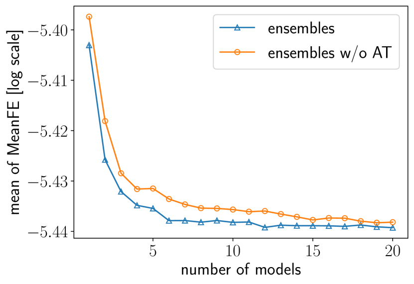
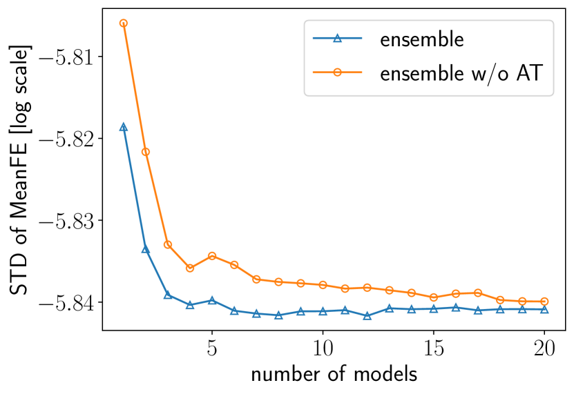
Figure 1: Accuracy. The horizontal-axis shows the number of NN in the ensembles. The mean and the STD of $18\,000$ testing samples are computed.

We evaluate the approach on the spectra simulation. We take the empirical variance as the baseline, which is commonly used in practice. Ensembles of NNs approximate the uncertainty from the empirical variance of multiple predictions. Usually, it uses mean square error (MSE) loss for the training. To simplify the comparison, we use the same models as the deep ensembles. We also compare the deep ensembles with a vanilla uncertainty estimation – measuring the uncertainty by the STD of a single model. Since the vanilla approach is the deep ensembles with $M=1$, we do not separately demonstrate the results. Additionally, we evaluate how the optional term, the AT, affects the ensembles.

We use the mean and max of fractional error metrics as in (Vogl, C. et al., 2020; Kerzendorf et al., 2021) to quantify the results:

$$\mathrm{MeanFE}= \frac{1}{N}\sum^{N}_{i=0}\frac{|\mathbf{y}^{\text{emu}}_{i}-\mathbf{y}^{\text{test}}_{i}|}{\mathbf{y}^{\text{test}}_{i}},$$

$$\mathrm{MaxFE}= \max^{N}_{i=0}\frac{|\mathbf{y}^{\text{emu}}_{i}-\mathbf{y}^{\text{test}}_{i}|}{\mathbf{y}^{\text{test}}_{i}},$$

where $N$ is the dimension of spectra, and $\mathbf{y}_{i}$ represents the flux at the $i$-th dimension.

3.1 Spectra prediction

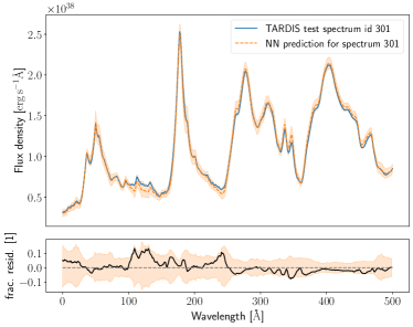
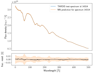
Figure 2: Examples of the uncertainty prediction. Highest and the lowest MaxFE from the test set predictions. The shaded areas denote 99.9 % confidence interval. In the lower figures, the black lines and dashed grey lines represent the residual and zero values, respectively.

Figure 1 shows the accuracy of the prediction. In general, the ensembles with ATs outperforms the approaches without ATs. With the number of models in the ensemble more than six, the accuracy is not significantly improved.

Based on the above evaluation, the AT hardly improves the uncertainty prediction, but it improves the accuracy, especially when the number of models is small. The deep ensembles outperform the empirical and vanilla approaches since the latter is easily over-confident. Taking into the accuracy, computation efficiency, and the uncertainty prediction into consideration, the best number of the models for the deep ensembles is suggested to be six. Figure 2 illustrates two examples of the prediction of the testing dataset using deep ensembles with six models and thus in the following we will use six models for the ensemble in our further tests.

3.2 Uncertainty prediction

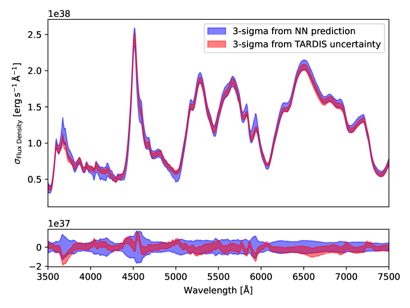
Figure 3: Comparison between the Monte Carlo uncertainty arising from TARDIS and the uncertainty estimated by the deep ensemble for test set sample 12625. We show $3-\sigma$ for visualization purposes.

The Dalek emulator has to contend with two types of uncertainties: 1) the prediction uncertainty stemming from a sparseness of sampling 2) the intrinsic uncertainty of the TARDIS simulator arising from the Monte Carlo radiative transfer. We have estimated the uncertainty given by TARDIS for the test-set spectrum with the highest $\max\sigma/\mu$-ratio (highest relative uncertainty; id=12625) and reran TARDIS (version hash ad91bef1a) with 100 different seeds to estimate the uncertainty arising from the Monte Carlo method. In Figure 3, we show that the network predicts a larger uncertainty that likely includes additional prediction uncertainty and mostly completely envelops the uncertainty given by TARDIS. Further tests are needed with a larger number of samples to explore the consistency of this result.

4 Conclusions

We present a probabilistic neural network model for the TARDIS supernova radiative transfer code. The emulator model is based on the deep ensemble approach given by (Lakshminarayanan et al., 2017) and even for a single model provides a MeanFE of $\approx 10^{-5}$ which is better than the model in the original Dalek emulator (MeanFe $\approx 10^{-3}$; Kerzendorf et al., 2021). In Figure 1, we show that for this architecture there is no substantial increase in accuracy with more than six models. We show that the test set TARDIS spectrum lies well within the predicted uncertainties (see Figure 3). We also show that (for now for a limited set) the uncertainty predicted by the neural network also captures the Monte Carlo uncertainty by TARDIS well. The preliminary work that is shown is very promising but still demands several more tests. As discussed in the introduction, the described work is part of a larger effort to build an active learning emulator for TARDIS with the express goal of doing supernova tomography and will be explored in future work.

Appendix A Contributor Role Taxonomy

We will use the Contributor Role Taxonomy as outlined in https://credit.niso.org/.

• Conceptualization: van der Smagt, Kerzendorf, Chen

• Formal Analysis: Chen, Kerzendorf

• Funding acquisition: van der Smagt, Kerzendorf

• Investigation: Chen, van der Smagt, Kerzendorf

• Methodology: Chen, van der Smagt

• Project administration: van der Smagt, Chen, Kerzendorf

• Software: Chen, Kerzendorf, van der Smagt, O’Brien

• Supervision: Kerzendorf, van der Smagt

• Writing - original draft: Chen, Kerzendorf

• Writing - review & editing: Chen, Kerzendorf, Buchner

Appendix B Acknowledgements

This research made use of TARDIS, a community-developed software package for spectral synthesis in supernovae (Kerzendorf & Sim, 2014; Kerzendorf et al., 2022a). The development of TARDIS received support from GitHub, the Google Summer of Code initiative, and from ESA’s Summer of Code in Space program. TARDIS is a fiscally sponsored project of NumFOCUS. TARDIS makes extensive use of Astropy (Astropy Collaboration et al., 2013, 2018; The Astropy Collaboration et al., 2022), pandas (Reback et al., 2022), and Numpy (Harris et al., 2020).

References

- Astropy Collaboration et al. (2013) Astropy Collaboration, Robitaille, T. P., Tollerud, E. J., Greenfield, P., Droettboom, M., Bray, E., Aldcroft, T., Davis, M., Ginsburg, A., Price-Whelan, A. M., Kerzendorf, W. E., Conley, A., Crighton, N., Barbary, K., Muna, D., Ferguson, H., Grollier, F., Parikh, M. M., Nair, P. H., Unther, H. M., Deil, C., Woillez, J., Conseil, S., Kramer, R., Turner, J. E. H., Singer, L., Fox, R., Weaver, B. A., Zabalza, V., Edwards, Z. I., Azalee Bostroem, K., Burke, D. J., Casey, A. R., Crawford, S. M., Dencheva, N., Ely, J., Jenness, T., Labrie, K., Lim, P. L., Pierfederici, F., Pontzen, A., Ptak, A., Refsdal, B., Servillat, M., and Streicher, O. Astropy: A community Python package for astronomy. Astronomy and Astrophysics, 558:A33, October 2013. doi: 10.1051/0004-6361/201322068. URL http://dx.doi.org/10.1051/0004-6361/201322068.
- Astropy Collaboration et al. (2018) Astropy Collaboration, Price-Whelan, A. M., Sipőcz, B. M., Günther, H. M., Lim, P. L., Crawford, S. M., Conseil, S., Shupe, D. L., Craig, M. W., Dencheva, N., Ginsburg, A., VanderPlas, J. T., Bradley, L. D., Pérez-Suárez, D., de Val-Borro, M., Aldcroft, T. L., Cruz, K. L., Robitaille, T. P., Tollerud, E. J., Ardelean, C., Babej, T., Bach, Y. P., Bachetti, M., Bakanov, A. V., Bamford, S. P., Barentsen, G., Barmby, P., Baumbach, A., Berry, K. L., Biscani, F., Boquien, M., Bostroem, K. A., Bouma, L. G., Brammer, G. B., Bray, E. M., Breytenbach, H., Buddelmeijer, H., Burke, D. J., Calderone, G., Cano Rodríguez, J. L., Cara, M., Cardoso, J. V. M., Cheedella, S., Copin, Y., Corrales, L., Crichton, D., D’Avella, D., Deil, C., Depagne, É., Dietrich, J. P., Donath, A., Droettboom, M., Earl, N., Erben, T., Fabbro, S., Ferreira, L. A., Finethy, T., Fox, R. T., Garrison, L. H., Gibbons, S. L. J., Goldstein, D. A., Gommers, R., Greco, J. P., Greenfield, P., Groener, A. M., Grollier, F., Hagen, A., Hirst, P., Homeier, D., Horton, A. J., Hosseinzadeh, G., Hu, L., Hunkeler, J. S., Ivezić, Ž., Jain, A., Jenness, T., Kanarek, G., Kendrew, S., Kern, N. S., Kerzendorf, W. E., Khvalko, A., King, J., Kirkby, D., Kulkarni, A. M., Kumar, A., Lee, A., Lenz, D., Littlefair, S. P., Ma, Z., Macleod, D. M., Mastropietro, M., McCully, C., Montagnac, S., Morris, B. M., Mueller, M., Mumford, S. J., Muna, D., Murphy, N. A., Nelson, S., Nguyen, G. H., Ninan, J. P., Nöthe, M., Ogaz, S., Oh, S., Parejko, J. K., Parley, N., Pascual, S., Patil, R., Patil, A. A., Plunkett, A. L., Prochaska, J. X., Rastogi, T., Reddy Janga, V., Sabater, J., Sakurikar, P., Seifert, M., Sherbert, L. E., Sherwood-Taylor, H., Shih, A. Y., Sick, J., Silbiger, M. T., Singanamalla, S., Singer, L. P., Sladen, P. H., Sooley, K. A., Sornarajah, S., Streicher, O., Teuben, P., Thomas, S. W., Tremblay, G. R., Turner, J. E. H., Terrón, V., van Kerkwijk, M. H., de la Vega, A., Watkins, L. L., Weaver, B. A., Whitmore, J. B., Woillez, J., Zabalza, V., and Astropy Contributors. The Astropy Project: Building an Open-science Project and Status of the v2.0 Core Package. The Astronomical Journal, 156:123, September 2018. ISSN 0004-6256. doi: 10.3847/1538-3881/aabc4f. URL https://ui.adsabs.harvard.edu/abs/2018AJ....156..123A.
- Blundell et al. (2015) Blundell, C., Cornebise, J., Kavukcuoglu, K., and Wierstra, D. Weight uncertainty in neural network. In International Conference on Machine Learning, pp. 1613–1622. PMLR, 2015.
- Cranmer et al. (2020) Cranmer, K., Brehmer, J., and Louppe, G. The frontier of simulation-based inference. Proceedings of the National Academy of Sciences, 117(48):30055–30062, 2020. doi: 10.1073/pnas.1912789117.
- Gal & Ghahramani (2016) Gal, Y. and Ghahramani, Z. Dropout as a bayesian approximation: Representing model uncertainty in deep learning. In international conference on machine learning, pp. 1050–1059. PMLR, 2016.
- Gneiting & Raftery (2007) Gneiting, T. and Raftery, A. E. Strictly proper scoring rules, prediction, and estimation. Journal of the American statistical Association, 102(477):359–378, 2007.
- Goodfellow et al. (2015) Goodfellow, I. J., Shlens, J., and Szegedy, C. Explaining and harnessing adversarial examples. ICLR, 2015.
- Guo et al. (2017) Guo, C., Pleiss, G., Sun, Y., and Weinberger, K. Q. On calibration of modern neural networks. In International Conference on Machine Learning, pp. 1321–1330. PMLR, 2017.
- Harris et al. (2020) Harris, C. R., Millman, K. J., van der Walt, S. J., Gommers, R., Virtanen, P., Cournapeau, D., Wieser, E., Taylor, J., Berg, S., Smith, N. J., Kern, R., Picus, M., Hoyer, S., van Kerkwijk, M. H., Brett, M., Haldane, A., del Río, J. F., Wiebe, M., Peterson, P., Gérard-Marchant, P., Sheppard, K., Reddy, T., Weckesser, W., Abbasi, H., Gohlke, C., and Oliphant, T. E. Array programming with NumPy. Nature, 585:357–362, September 2020. ISSN 0028-0836. doi: 10.1038/s41586-020-2649-2. URL https://ui.adsabs.harvard.edu/abs/2020Natur.585..357H.
- He et al. (2016) He, K., Zhang, X., Ren, S., and Sun, J. Deep residual learning for image recognition. In Proceedings of the IEEE conference on computer vision and pattern recognition, pp. 770–778, 2016.
- Kerzendorf et al. (2022a) Kerzendorf, W., Sim, S., Vogl, C., Williamson, M., Pássaro, E., Flörs, A., Camacho, Y., Jančauskas, V., Harpole, A., Nöbauer, U., Lietzau, S., Mishin, M., Tsamis, F., Boyle, A., Shingles, L., Gupta, V., Desai, K., Klauser, M., Beaujean, F., Suban-Loewen, A., Heringer, E., Barna, B., Gautam, G., Fullard, A., Cawley, K., Singhal, J., Smith, I., Barbosa, T., Sondhi, D., Patel, M., Varanasi, K., Gillanders, J., Arya, A., O’Brien, J., Eweis, Y., Reinecke, M., Bylund, T., Bentil, L., Savel, A., Yu, J., Eguren, J., Alam, A., Magee, M., Livneh, R., Rajagopalan, S., Mishra, S., Reichenbach, J., Jain, R., Floers, A., Brar, A., Singh, S., Talegaonkar, C., Kowalski, N., Selsing, J., Sofiatti, C., Aggarwal, Y., Sarafina, N., Patra, N., Singh Rathore, P., Patel, P., Sharma, S., Gupta, S., Wahi, U., Sandler, M., Volodin, D., Dasgupta, D., Yap, K., Kharkar, A., Nayak U, A., Kolliboyina, C., and Kumar, A. tardis-sn/tardis: Tardis v2022.4.1, April 2022a. URL https://doi.org/10.5281/zenodo.6430631.
- Kerzendorf et al. (2022b) Kerzendorf, W., Sim, S., Vogl, C., Williamson, M., Pássaro, E., Flörs, A., Camacho, Y., Jančauskas, V., Harpole, A., Nöbauer, U., Lietzau, S., Mishin, M., Tsamis, F., Boyle, A., Shingles, L., Gupta, V., Desai, K., Klauser, M., Beaujean, F., Suban-Loewen, A., Heringer, E., Barna, B., Gautam, G., Fullard, A., Cawley, K., Smith, I., Singhal, J., Arya, A., Sondhi, D., Barbosa, T., Yu, J., Patel, M., O’Brien, J., Varanasi, K., Gillanders, J., Savel, A., Reinecke, M., Eweis, Y., Bylund, T., Bentil, L., Eguren, J., Alam, A., Bartnik, M., Magee, M., Shields, J., Livneh, R., Rajagopalan, S., Chitchyan, S., Mishra, S., Reichenbach, J., Jain, R., Floers, A., Brar, A., Singh, S., Selsing, J., Sofiatti, C., Talegaonkar, C., Bot, T., Kowalski, N., Yap, K., Patel, P., Sharma, S., Prasad, S., Venkat, S., Dasgupta, D., Zaheer, M., Gupta, S., Volodin, D., Patra, N., Singh Rathore, P., Lemoine, T., Sarafina, N., Kolliboyina, C., Sandler, M., Nayak U, A., Aggarwal, Y., Kumar, A., Holas, A., Kharkar, A., kumar, a., and Wahi, U. tardis-sn/tardis: Tardis v2022.05.08, May 2022b. URL https://doi.org/10.5281/zenodo.6527890.
- Kerzendorf & Sim (2014) Kerzendorf, W. E. and Sim, S. A. A spectral synthesis code for rapid modelling of supernovae. MNRAS, 440:387–404, May 2014. doi: 10.1093/mnras/stu055.
- Kerzendorf et al. (2021) Kerzendorf, W. E., Vogl, C., Buchner, J., Contardo, G., Williamson, M., and van der Smagt, P. Dalek: A deep learning emulator for tardis. The Astrophysical Journal Letters, 910(2):L23, 2021.
- Lakshminarayanan et al. (2017) Lakshminarayanan, B., Pritzel, A., and Blundell, C. Simple and scalable predictive uncertainty estimation using deep ensembles. In Advances in Neural Information Processing Systems, volume 30. Curran Associates, Inc., 2017.
- Liu et al. (2020) Liu, J., Lin, Z., Padhy, S., Tran, D., Bedrax Weiss, T., and Lakshminarayanan, B. Simple and principled uncertainty estimation with deterministic deep learning via distance awareness. In Larochelle, H., Ranzato, M., Hadsell, R., Balcan, M. F., and Lin, H. (eds.), Advances in Neural Information Processing Systems, volume 33, pp. 7498–7512. Curran Associates, Inc., 2020.
- O’Brien et al. (2021) O’Brien, J. T., Kerzendorf, W. E., Fullard, A., Williamson, M., Pakmor, R., Buchner, J., Hachinger, S., Vogl, C., Gillanders, J. H., Flörs, A., and van der Smagt, P. Probabilistic Reconstruction of Type Ia Supernova SN 2002bo. ApJ Letter, 916(2):L14, August 2021. doi: 10.3847/2041-8213/ac1173.
- Ovadia et al. (2019) Ovadia, Y., Fertig, E., Ren, J., Nado, Z., Sculley, D., Nowozin, S., Dillon, J., Lakshminarayanan, B., and Snoek, J. Can you trust your model's uncertainty? evaluating predictive uncertainty under dataset shift. In Advances in Neural Information Processing Systems, volume 32. Curran Associates, Inc., 2019.
- Paszke et al. (2019) Paszke, A., Gross, S., Massa, F., Lerer, A., Bradbury, J., Chanan, G., Killeen, T., Lin, Z., Gimelshein, N., Antiga, L., Desmaison, A., Kopf, A., Yang, E., DeVito, Z., Raison, M., Tejani, A., Chilamkurthy, S., Steiner, B., Fang, L., Bai, J., and Chintala, S. Pytorch: An imperative style, high-performance deep learning library. In Advances in Neural Information Processing Systems 32, pp. 8024–8035. Curran Associates, Inc., 2019.
- Pedregosa et al. (2011) Pedregosa, F., Varoquaux, G., Gramfort, A., Michel, V., Thirion, B., Grisel, O., Blondel, M., Prettenhofer, P., Weiss, R., Dubourg, V., et al. Scikit-learn: Machine learning in python. the Journal of machine Learning research, 12:2825–2830, 2011.
- Reback et al. (2022) Reback, J., jbrockmendel, McKinney, W., den Bossche, J. V., Roeschke, M., Augspurger, T., Hawkins, S., Cloud, P., gfyoung, Sinhrks, Hoefler, P., Klein, A., Petersen, T., Tratner, J., She, C., Ayd, W., Naveh, S., Darbyshire, J., Shadrach, R., Garcia, M., Schendel, J., Hayden, A., Saxton, D., Gorelli, M. E., Li, F., Wörtwein, T., Zeitlin, M., Jancauskas, V., McMaster, A., and Li, T. pandas-dev/pandas: Pandas 1.4.3, June 2022. URL https://doi.org/10.5281/zenodo.6702671.
- Szegedy et al. (2014) Szegedy, C., Zaremba, W., Sutskever, I., Bruna, J., Erhan, D., Goodfellow, I., and Fergus, R. Intriguing properties of neural networks. In International Conference on Learning Representations, 2014.
- The Astropy Collaboration et al. (2022) The Astropy Collaboration, Price-Whelan, A. M., Lian Lim, P., Earl, N., Starkman, N., Bradley, L., Shupe, D. L., Patil, A. A., Corrales, L., Brasseur, C. E., Nöthe, M., Donath, A., Tollerud, E., Morris, B. M., Ginsburg, A., Vaher, E., Weaver, B. A., Tocknell, J., Jamieson, W., van Kerkwijk, M. H., Robitaille, T. P., Merry, B., Bachetti, M., Günther, H. M., Aldcroft, T. L., Alvarado-Montes, J. A., Archibald, A. M., Bódi, A., Bapat, S., Barentsen, G., Bazán, J., Biswas, M., Boquien, M., Burke, D. J., Cara, D., Cara, M., E Conroy, K., Conseil, S., Craig, M. W., Cross, R. M., Cruz, K. L., D’Eugenio, F., Dencheva, N., Devillepoix, H. A. R., Dietrich, J. P., Davis Eigenbrot, A., Erben, T., Ferreira, L., Foreman-Mackey, D., Fox, R., Freij, N., Garg, S., Geda, R., Glattly, L., Gondhalekar, Y., Gordon, K. D., Grant, D., Greenfield, P., Groener, A. M., Guest, S., Gurovich, S., Handberg, R., Hart, A., Hatfield-Dodds, Z., Homeier, D., Hosseinzadeh, G., Jenness, T., Jones, C. K., Joseph, P., Bryce Kalmbach, J., Karamehmetoglu, E., Kałuszyński, M., Kelley, M. S. P., Kern, N., Kerzendorf, W. E., Koch, E. W., Kulumani, S., Lee, A., Ly, C., Ma, Z., MacBride, C., Maljaars, J. M., Muna, D., Murphy, N. A., Norman, H., O’Steen, R., Oman, K. A., Pacifici, C., Pascual, S., Pascual-Granado, J., Patil, R. R., Perren, G. I., Pickering, T. E., Rastogi, T., Roulston, B. R., Ryan, D. F., Rykoff, E. S., Sabater, J., Sakurikar, P., Salgado, J., Sanghi, A., Saunders, N., Savchenko, V., Schwardt, L., Seifert-Eckert, M., Shih, A. Y., Shrey Jain, A., Shukla, G., Sick, J., Simpson, C., Singanamalla, S., Singer, L. P., Singhal, J., Sinha, M., Sipőcz, B. M., Spitler, L. R., Stansby, D., Streicher, O., Šumak, J., Swinbank, J. D., Taranu, D. S., Tewary, N., Tremblay, G. R., de Val-Borro, M., Van Kooten, S. J., Vasović, Z., Verma, S., Cardoso, J. V. d. M., Williams, P. K. G., Wilson, T. J., Winkel, B., Wood-Vasey, W. M., Xue, R., Yoachim, P., ZHANG, C., and Zonca, A. The Astropy Project: Sustaining and Growing a Community-oriented Open-source Project and the Latest Major Release (v5.0) of the Core Package, June 2022. URL https://ui.adsabs.harvard.edu/abs/2022arXiv220614220T.
- Van Amersfoort et al. (2020) Van Amersfoort, J., Smith, L., Teh, Y. W., and Gal, Y. Uncertainty estimation using a single deep deterministic neural network. In International Conference on Machine Learning, pp. 9690–9700. PMLR, 2020.