BP-Im2col: Implicit Im2col Supporting AI Backpropagation on Systolic Arrays*

Abstract

State-of-the-art systolic array-based accelerators adopt the traditional im2col algorithm to accelerate the inference of convolutional layers. However, traditional im2col cannot efficiently support AI backpropagation. Backpropagation in convolutional layers involves performing transposed convolution and dilated convolution, which usually introduces plenty of zero-spaces into the feature map or kernel. The zero-space data reorganization interfere with the continuity of training and incur additional and non-negligible overhead in terms of off- and on-chip storage, access and performance. Since countermeasures for backpropagation are rarely proposed, we propose BP-im2col, a novel im2col algorithm for AI backpropagation, and implement it in RTL on a TPU-like accelerator. Experiments on TPU-like accelerator indicate that BP-im2col reduces the backpropagation runtime by 34.9% on average, and reduces the bandwidth of off-chip memory and on-chip buffers by at least 22.7% and 70.6% respectively, over a baseline accelerator adopting the traditional im2col. It further reduces the additional storage overhead in the backpropagation process by at least 74.78%.

I Introduction

State-of-the-art neural network accelerators adopt systolic arrays [1] to accelerate the inference and training of convolutional neural networks (CNNs) [2, 3, 4, 5]. The existing systolic array-based accelerators largely adopt the traditional im2col algorithm [6] to lower the inference of convolutional layers to general matrix multiplication (GEMM). Backpropagation in convolutional layers involves performing more complicated transposed convolution and dilated convolution, which is necessary to perform zero-insertions and zero-paddings (collectively referred to as zero-spaces) for the feature map or kernel. According to our analysis, for convolutional layers with $stride\geq 2$, the zero-spaces cause the sparsity of the lowered matrix to be as high as about 75%.

Existing accelerators [2, 3, 4, 5] use the same systolic array-based platforms to speed up the inference and training of convolutional layers. The core idea of solving zero-space of the input or kernel on systolic array-based platforms is to pre-process them to be zero-inserted and zero-padded in advance [7]. However, the data reorganization requires large amounts of memory access and interferes with the continuity of training. Even though part of the latency of data reorganization can be hidden in the training process as a whole, it nevertheless increases the complexity of hardware control. The transmission of zero-spaces also leads to very high bandwidth requirements, which is more obvious for processors with mismatched bandwidth and computing power. Therefore, it is essential for the im2col algorithm to integrate zero-skipping mechanism. Besides, explicit im2col generates and stores a matrix-like copy of the input and kernel to facilitate further matrix multiplication by PEs, which also incurs significant performance and memory overhead for the convolution itself. This disadvantage can be avoided through the use of the implicit im2col.

While numerous publicly available methods [8, 9, 10] describing the im2col algorithm only support the inference of convolutional layers, countermeasures for the backpropagation are rarely proposed. Our contributions are summarized as follows:

• We propose a novel implicit im2col algorithm, named BP-im2col, which completely eliminates the zero-space data reorganization during backpropagation;

• We design and implement a TPU-like accelerator, integrated with the hardware implementation of BP-im2col. The address generation modules achieve low-overhead Non-Zero detection and avoid data reorganization during training;

• The proposed TPU-like accelerator reduces the backpropagation runtime by 34.9% on average, and reduces the bandwidth of off-chip memory and on-chip buffers by at least 22.7% and 70.6% respectively, over a baseline accelerator adopting the traditional im2col. It also reduces the additional storage overhead in the backpropagation process.

For clarity, TABLE I shows the meaning of the symbols used in this article.

II Backpropagation of CNN

The backpropagation involves calculating the loss of the input and the gradient of the kernel. Equation 1 outlines the training process [3, 2]. After expressing the convolution as a matrix multiplication ($Y=A\times B$) via im2col [6], the huge benefit of the very regular memory access pattern produces a high ratio of floating-point operations per byte of data transferred.

$$inference: \quad I^{l+1}=I^{l}_{e}\ast W^{l}$$ (1)

$$loss: \quad\delta I^{l}=\delta I^{l+1}_{ei}\ast Tr(rot_{180^{\circ}}{W^{l}})$$

$$gradient: \quad Tr(\delta W^{l})=Tr(I^{l}_{e})\ast Tr(\delta I^{l+1}_{i})$$

TABLE I: Meaning of symbols.

Symbol	Meaning
$I^{l},W^{l}$	Input and kernel of the $l$-th convolutional layer.
$\delta I^{l},\delta W^{l}$	The loss of $I^{l}$ and the gradient of $W^{l}$.
$\ast,rot_{180^{\circ}}$	Convolution symbol, $180^{\circ}$ kernel-wise rotation.
$Tr(\cdot)$	Transpose the first two dimensions of $4d$ tensors.
$e/i/ei$	Zero-paddings, zero-insertions, and both.
$B,C,H_{i},W_{i}$	Batch size, input channel, height and width of $I^{l}$.
$N,K_{h},K_{w}$	Output channel, height and width of $W^{l}$.
$H_{o},W_{o}$	Height and width of the output $I^{l+1}$.
$S,P_{h},P_{w}$	Stride, padding in height and width directions.
$H_{o}^{\prime\prime}$	$H_{o}+(H_{o}-1)\cdot(S-1)$.
$W_{o}^{\prime\prime}$	$W_{o}+(W_{o}-1)\cdot(S-1)$.
$H_{o}^{\prime\prime\prime}$	$H_{o}+2(K_{h}-1-P_{h})+(H_{o}-1)\cdot(S-1)$.
$W_{o}^{\prime\prime\prime}$	$W_{o}+2(K_{w}-1-P_{w})+(W_{o}-1)\cdot(S-1)$.

II-1 Loss calculation

The difference between loss calculation and inference is that loss calculation is realized by performing transposed convolution on the loss of the output by the convolving kernel (see Equation 1). Another important difference is that the stride of the transposed convolution is a fixed value of $1$. The transposed convolution and the im2col process of loss calculation are illustrated in Fig. 1 and Fig. 2. It can be observed that zero-insertions and zero-paddings of the loss of the output result in more zero pixels in the convoluted feature map. The combination of zero-paddings and zero-insertions introduces a huge amount of zero pixels to matrix $B$ after im2col, and the ratio of zero pixels is as high as 75% to 93.91% for popular convolutional neural networks.

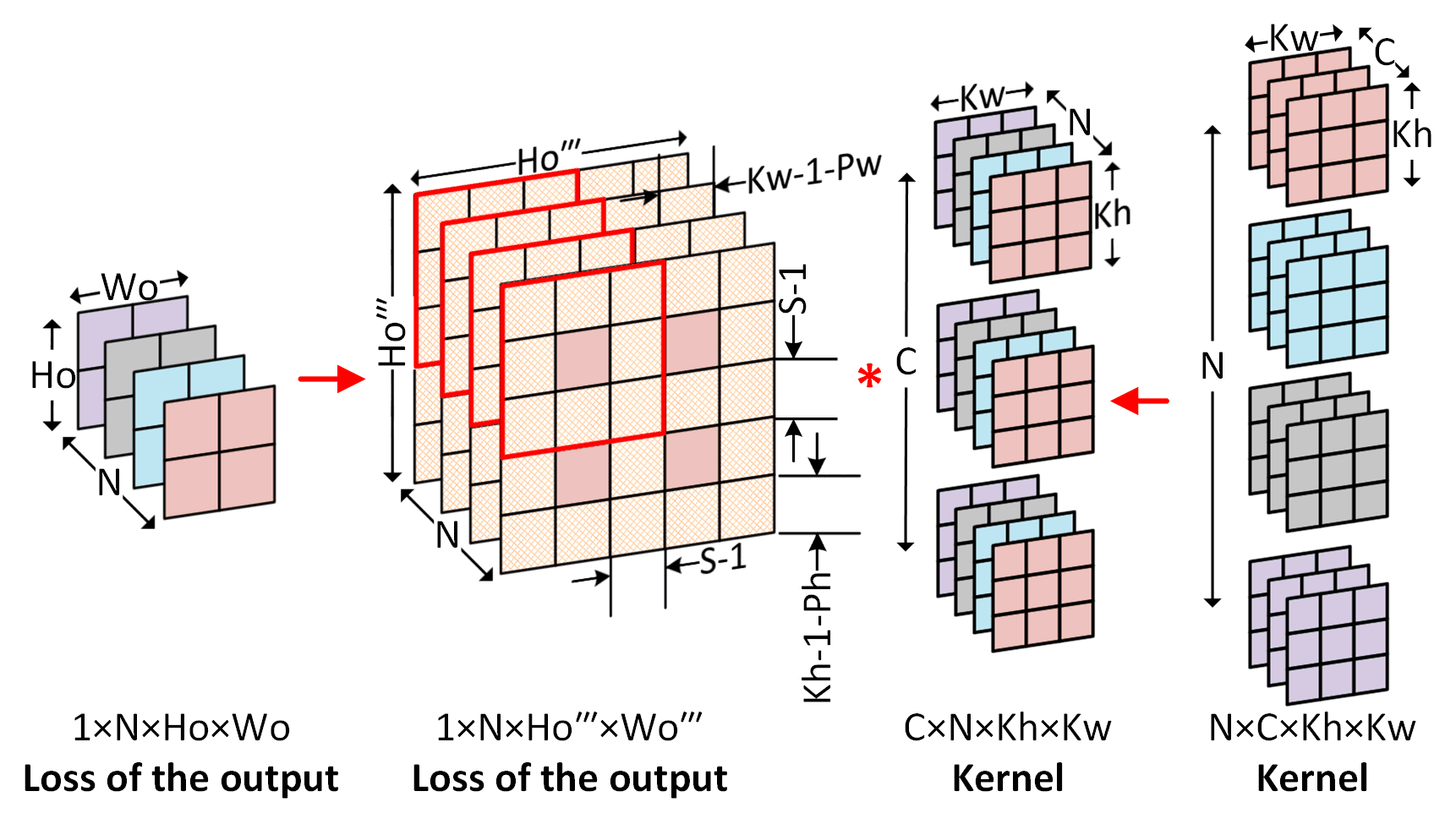
Figure 1: Loss calculation of convolutional layers.

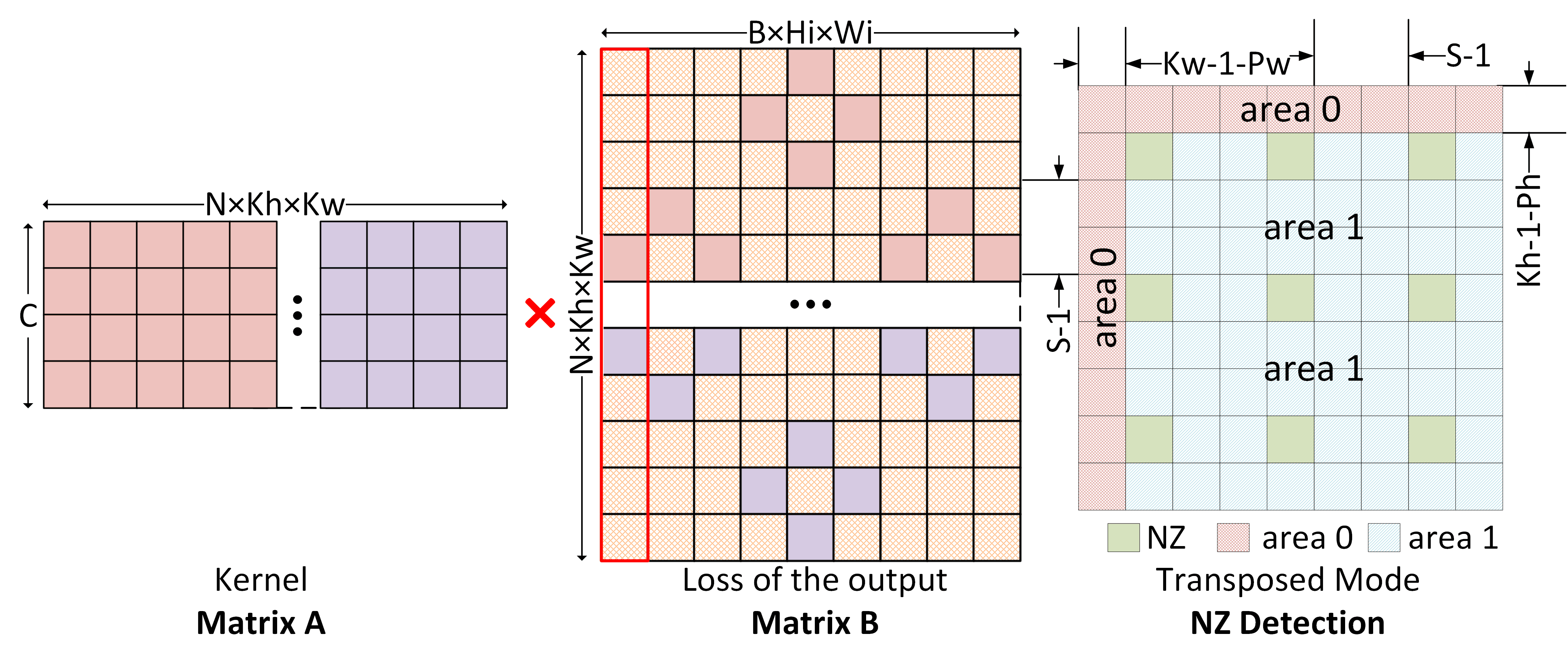
Figure 2: Traditional im2col of loss calculation and NZ detection of transposed mode. The data of matrix B marked by the red boxes in Fig. 1 is expanded into the column marked by the red box in Fig. 2.

II-2 Gradient Calculation

The gradient calculation is realized by performing dilated convolution on the reorganized input by the reorganized loss of the output (see Equation 1). As with the loss calculation, the stride of the dilated convolution is a fixed value of $1$. We detail the reorganized steps of the input and the loss of the output in Fig. 3, while Fig. 4 illustrates the im2col process for gradient calculation. The number of zeros introduced by the zero-padding of the input is roughly the same as that introduced by the inference. What causes the overall plenty of zeros is the zero-insertions for the loss of the output. The zero pixels caused by zero-insertions for the loss of the output is extremely large, and the ratio of zero pixels is as high as 74.8% to 93.6% for popular convolutional neural networks.

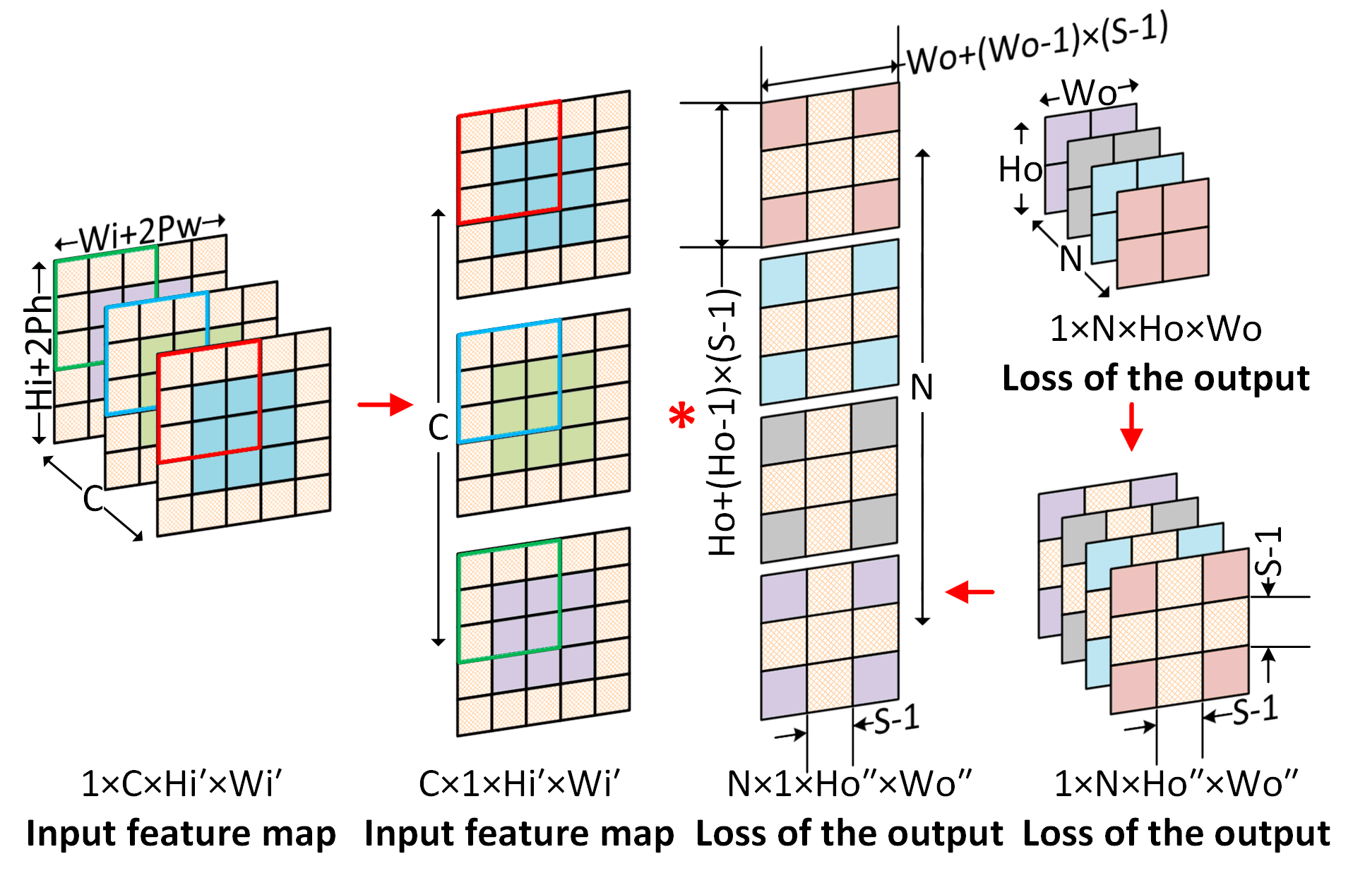
Figure 3: Gradient calculation of convolutional layers.

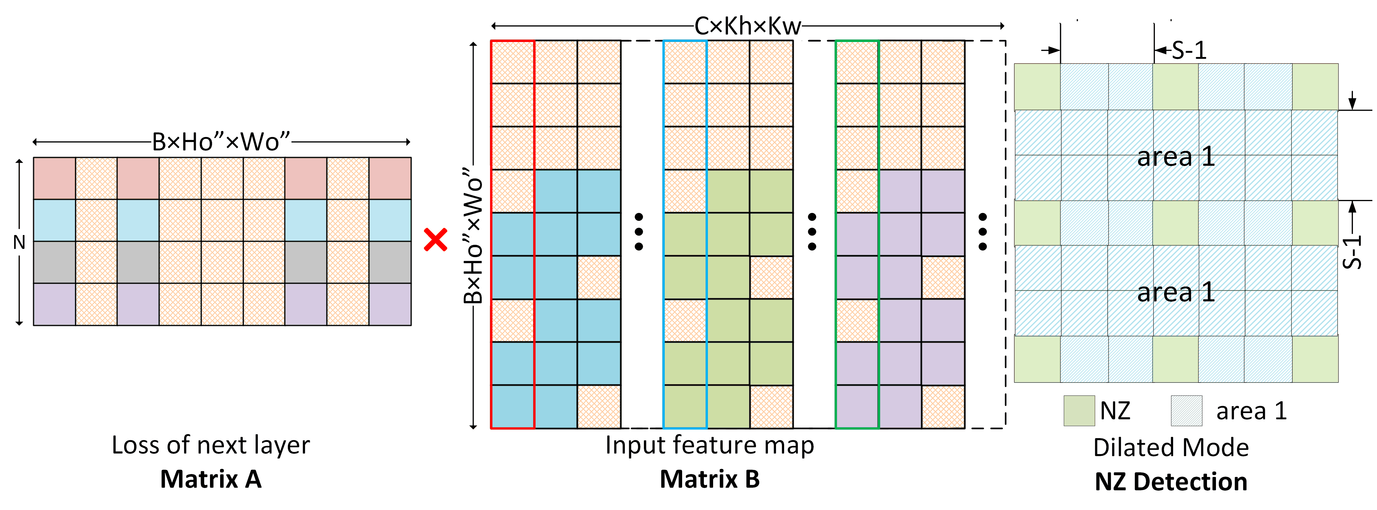
Figure 4: Traditional im2col of gradient calculation and NZ detection of dilated mode. The data of matrix B marked by the colored boxes in Fig. 3 is expanded into the column marked by the colored box in Fig. 4.

III Algorithm and Hardware Design

III-A Address Generation of BP-Im2col

When performing BP-im2col for loss calculation, we maintain a virtual matrix $B$ along with a virtual four-dimensional convoluted feature map with zero-spaces. We map the addresses of virtual matrix $B$ to the virtual four-dimensional convoluted feature map with zero-spaces, and then map it to the four-dimensional convoluted feature map without zero-spaces, which is actually stored in the on-chip buffer. For gradient calculation, the mapping of matrix $A$ with zero-spaces is similar to matrix $B$, except that it does not need to perform im2col and has only zero-insertions. Fig. 5 describes the address mapping of matrix $A$ and matrix $B$.

III-B NZ Detection

III-B1 Transposed convolution mode

For loss calculation, we divide the zero pixels in a single channel into two areas: namely, one is composed of upper and left zero-paddings (area $0$), while the other is composed of other zero-spaces (area $1$), which is shown in Fig. 2. The condition that a pixel $(h,w)$ is in area $0$ is:

$$\small\vspace{-0.2cm}h<K_{h}-1-P_{h}\ or\ w<K_{w}-1-P_{w}.\vspace{-0.1cm}$$ (2)

Moreover, the condition that the pixel is in area $1$ is:

$$\small\vspace{-0.1cm}[h-(K_{h}-1-P_{h})]\%S>0\ or\ [w-(K_{w}-1-P_{w})]\%S>0.\vspace{-0.1cm}$$ (3)

We present the address mapping algorithm of matrix $B$ lowered during loss calculation in Algorithm 1.

Input: Address of a pixel in virtual matrix $B$, $addr_{in}$;

Output: Address in the original feature map without zero-spaces, $addr_{out}$;

1 $row$, $col$ = $\lfloor addr_{in}/(B\cdot H_{i}\cdot W_{i})\rfloor$, $addr_{in}\%(B\cdot H_{i}\cdot W_{i})$;

2 $b$, $temp1$, $w_{k}$ = $\lfloor col/(H_{i}\cdot W_{i})\rfloor$, $\lfloor row/K_{w}\rfloor$, $row\%K_{w}$;

3 $n$, $h_{k}$, $temp2$ = $\lfloor temp1/K_{h}\rfloor$, $temp1\%K_{h}$, $col\%(H_{i}\cdot W_{i})$;

4 $h,w$ = $\lfloor temp2/Wi\rfloor+h_{k}$, $temp2\%Wi+w_{k}$;

5 if $(h,w)$ satisfy Equation 2 or Equation 3 then

6       $addr_{out}$ = $NULL$; //Zero-spaces.

7else

8       $h^{{}^{\prime}}$, $w^{{}^{\prime}}$ = $(h-(K_{h}-1-P_{h}),w-(K_{w}-1-P_{w}))/S$;

9       $addr_{out}$ = $b\cdot N\cdot H_{o}\cdot W_{o}+n\cdot H_{o}\cdot W_{o}+h^{{}^{\prime}}\cdot W_{o}+w^{{}^{\prime}}$;

10      

11 end if

Algorithm 1 BP-im2col of transposed mode.

III-B2 Dilated convolution mode

Assuming that a certain pixel to be calculated is mapped to the position of the virtual convolving kernel with zero-insertions as $(h,w)$, the position of the pixel in the channel is shown in Fig. 2. The condition that this pixel to be located in the zero pixel area (area $1$) is:

$$\small\vspace{-0.2cm}h\%S>0\ or\ w\%S>0.$$ (4)

Moreover, its target position in the actually stored convolving kernel is $(h/S,w/S)$. We present the address mapping algorithm of matrix $A$ lowered during gradient calculation in Algorithm 2.

Input: Address of a pixel in virtual matrix $A$, $addr_{in}$;

Output: Address in original loss of the output without zero-insertions, $addr_{out}$;

1 $n$, $col$ = $\lfloor addr_{in}/(B\cdot H_{o}^{\prime\prime}\cdot W_{o}^{\prime\prime})\rfloor$, $addr_{in}\%(B\cdot H_{o}^{\prime\prime}\cdot W_{o}^{\prime\prime})$;

2 $temp$, $w$ = $\lfloor col/W_{o}^{\prime\prime}\rfloor$, $col\%W_{o}^{\prime\prime}$;

3 $b$, $h$ = $\lfloor temp/H_{o}^{\prime\prime}\rfloor$, $temp\%H_{o}^{\prime\prime}$;

4 if $(h,w)$ satisfy Equation 4 then

5       $addr_{out}$ = $NULL$; //Zero-insertions.

6else

7       $h^{{}^{\prime}}$, $w^{{}^{\prime}}$ = $(h,w)/S$;

8       $addr_{out}$ = $b\cdot N\cdot H_{o}\cdot W_{o}+n\cdot H_{o}\cdot W_{o}+h^{{}^{\prime}}\cdot W_{o}+w^{{}^{\prime}}$;

9      

10 end if

Algorithm 2 BP-im2col of dilated mode.

III-C Hardware Design

We implement a systolic array, named as TPU-like accelerator. It uses a $16\times 16$ systolic array as the acceleration core and adopts the input-stationary data flow. Fig. 5 illustrates the architectural details. Both buffer $A$ and buffer $B$ are double-buffered. Buffer $A$ supplies the data of the dynamic lowered matrix $A$ for PEs, while buffer $B$ supplies that of the stationary lowered matrix $B$. We design $16$ FIFOs with different depths between buffer $A$ and the systolic array to skew the data layout. To implement BP-im2col, we use address generation and compression logic to generate appropriate addresses for each block of matrix $A$ and matrix $B$, and recover the data format for the compressed data that is transmitted back.

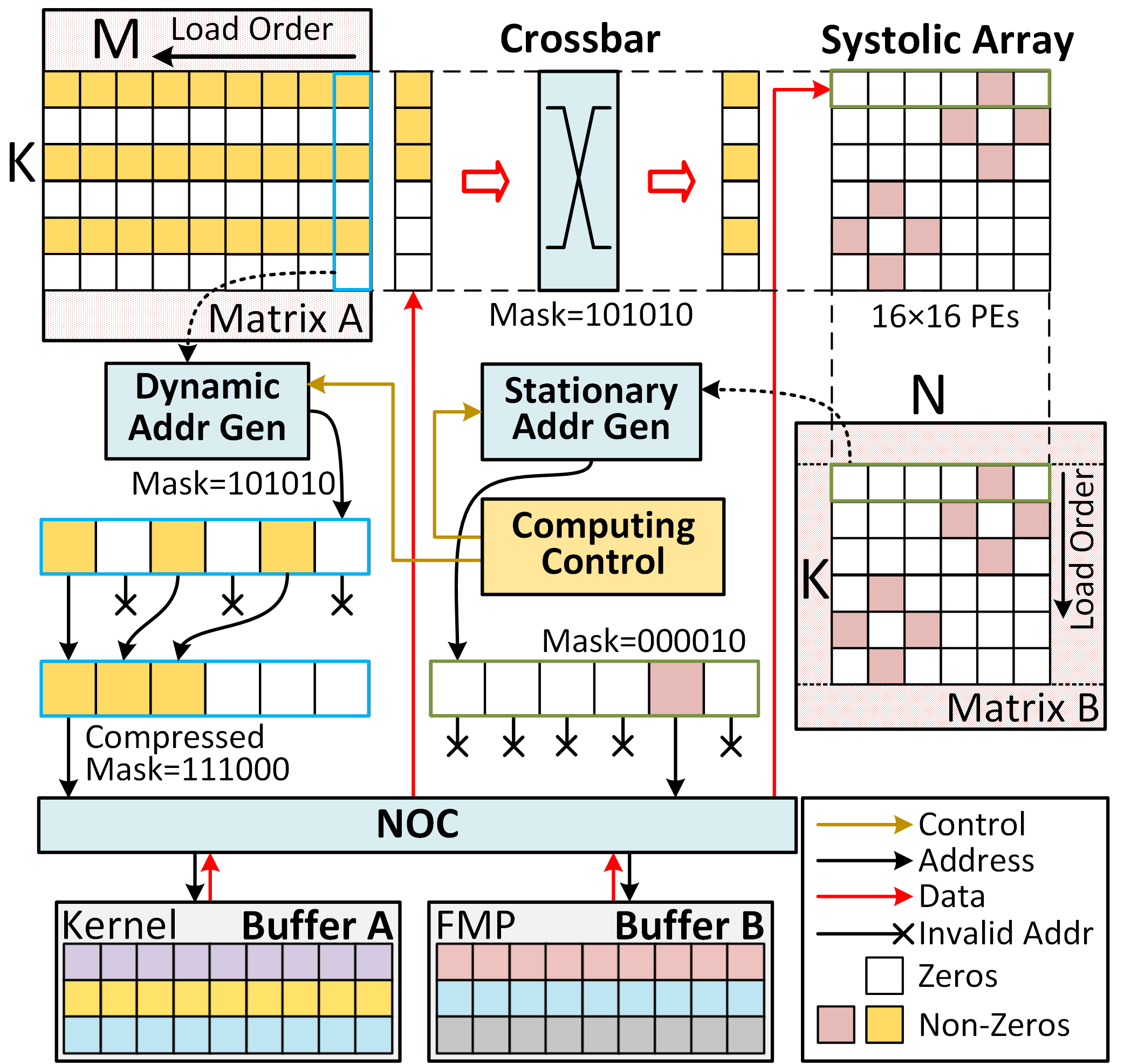
Figure 5: Address mapping and architecture of TPU-like.

Transposed convolution mode. In Fig. 5, we describe how a block of matrix $B$ is loaded onto the systolic array. The address generation module first generates pixel addresses under the virtual stationary matrix $B$ view and we take $16$ channels to generate addresses in parallel during the address generation of matrix $B$ to supply data for $16$ PEs in each row of the systolic array. We detect each address according to Section III-B to filter the zero pixels, and perform address mapping to generate the compressed address of the actually stored feature map. After the data is transmitted back, we send it directly to the PEs, according to its compressed mask. When the data enters the systolic array, the zero pixel position identified by the compressed mask is temporarily filled with zeros.

Dilated convolution mode. Fig. 5 also describes how a block of lowered matrix $A$ is loaded into the systolic array. The dynamic matrix address generation module generates addresses under the virtual dynamic matrix $A$ view. The addresses of the dynamic matrix $A$ are continuous; thus, we only generate the first address of the data in each row of blocks of matrix $A$ ($addr$), and the addresses of the $16$ elements in this row are: $addr$, $addr+1$, $\cdots$, $addr+15$. However, $16$ elements of a row block of matrix $A$ are not strictly continuously stored for dilated convolution, for the reason that there may be zeros that are not actually stored. We therefore need all addresses of the $16$ channels to perform address mapping and NZ detection to determine the non-zero position of the row elements. Although the mapped addresses of the $16$ elements in a row of matrix $A$ are not strictly consecutive, the non-zero elements are stored consecutively in buffer $A$. We compress the non-consecutive $16$ mapped element addresses and send only the address of the first non-zero element to buffer $A$. The data transmitted back by buffer $A$ is a continuous number of elements starting from the first non-zero element. Then we recover the data arrangement through a crossbar according to the original mask. Similarly, only the compressed addresses and non-zero data are passed on to the chip.

IV Evaluation

TPU-like Experiment Setup. We implement the traditional im2col [6] and BP-im2col on TPU-like accelerator. Our evaluation uses the $FP32$ data type and a batch size of $2$. The synthesis uses $ASAP7$, a 7 nm predictive PDK library [11].

Workload. We evaluate all convolutional layers with stride $\geq 2$ from several CNNs. The ”Original” legend in figures is referred to the adoption of traditional im2col integrated with zero-space reorganization, while the ”Ours” legend refers to the adoption of implicit BP-Im2col.

IV-A Overall Calculation Time

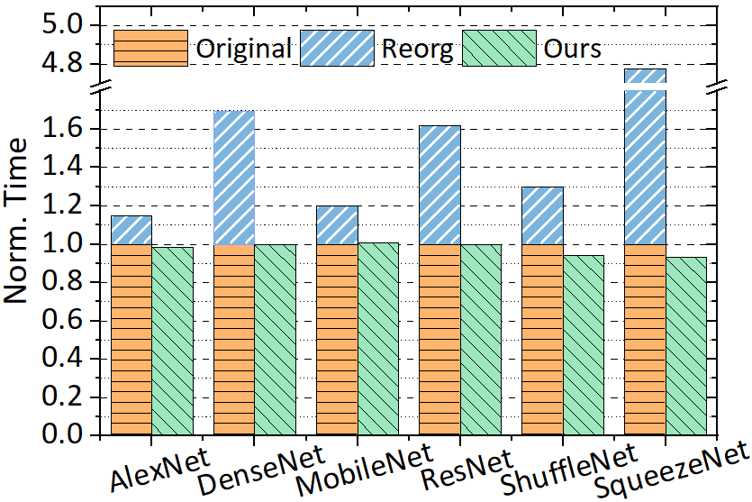
(a) Loss calculation.

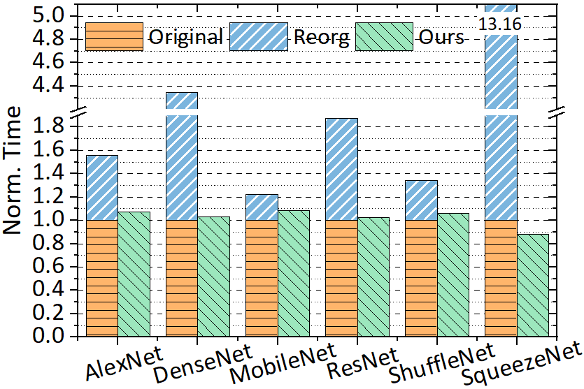
(b) Gradient calculation.

Figure 6: Performance comparison.

We recorded the performing time of loss calculation and gradient calculation during backpropagation. 6(a) demonstrates that BP-im2col significantly reduces the loss calculation time by 14.5%, 41.2%, 16.0%, 38.3%, 22.8% and 79.0% respectively, and that most of this gap stems from the data reorganization of zero-spaces. 6(b) demonstrates that the gradient calculation time of BP-im2col is reduced by 31.3%, 76.3%, 17.7%, 45.3%, 20.9% and 92.4% respectively. BP-im2col greatly reduces the performance overhead of loss calculation and gradient calculation caused by data reorganization. Table II also shows the runtime of loss calculation and gradient calculation of several convolutional layers.

TABLE II: Runtime of loss calculation and gradient calculation of several convolutional layers.

Convolution layers	Loss Calculation (cycles)				Grad Calculation (cycles)
$H_{i}(W_{i})/C/N/K_{h}(K_{w})/$	BP-im2col	Traditional im2col		Speedup	BP-im2col	Traditional im2col		Speedup
$S/P_{h}(P_{w})$		Computation	Reorganization			Computation	Reorganization
224/3/64/3/2/0	8962102	8929989	37083360	5.13$\times$	2416476	2274645	37083360	16.29$\times$
112/64/64/3/2/1	10310400	10329856	3798997	1.37$\times$	9439744	8905216	3798997	1.35$\times$
56/256/512/1/2/0	9330688	9125888	15592964	2.65$\times$	11653120	11636736	15592964	2.34$\times$
28/244/244/3/2/1	8081314	8222247	1657646	1.22$\times$	8575509	8089919	1657646	1.14$\times$
14/1024/2048/1/2/0	11984896	11059200	6074461	1.42$\times$	15278080	15245312	6074461	1.40$\times$

IV-B Off-chip Memory & Buffer Bandwidth Occupation

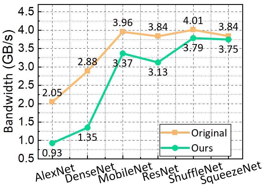
(a) Loss calculation.

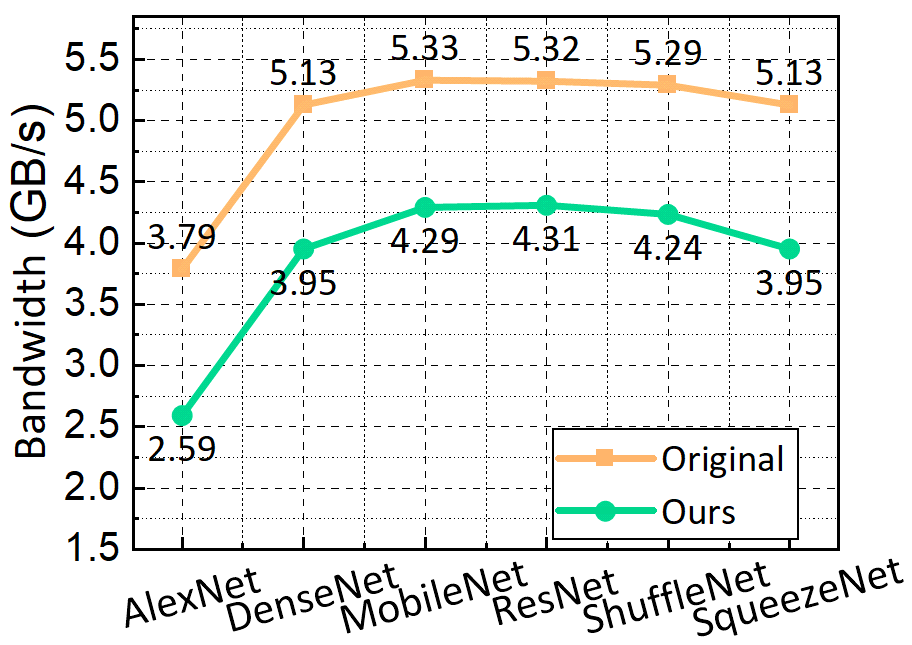
(b) Gradient calculation.

Figure 7: The bandwidth occupation of off-chip memory.

7(a) demonstrates that BP-im2col significantly reduces the bandwidth occupation of data transmission to buffer $B$ during loss calculation: specifically, it has a minimum reduction of 2.34% (for SqueezeNet) and a maximum reduction of 54.63% (for AlexNet). 7(b) further demonstrates that BP-im2col significantly reduces the bandwidth occupation of data transmission to buffer $A$ during gradient calculation: specifically, it has a minimum reduction of 18.98% (for ResNet) and a maximum reduction of 31.66% (for AlexNet).

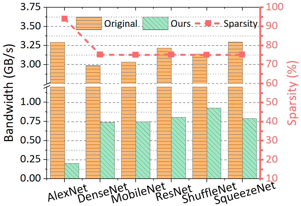
(a) Bandwidth of buffer B during     loss calculation.

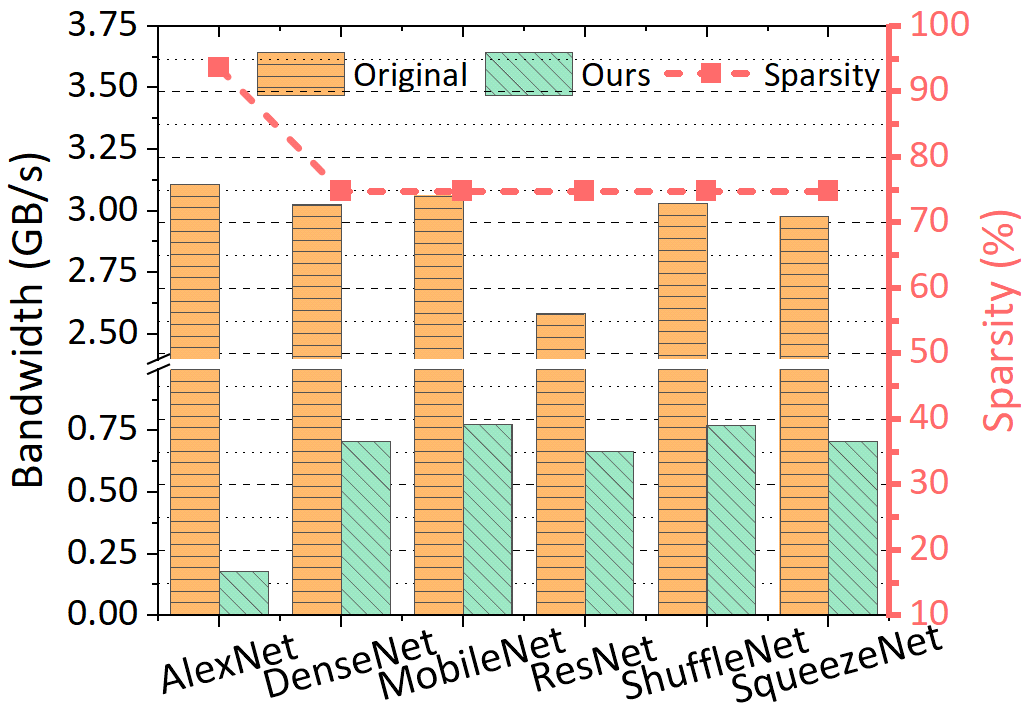
(b) Bandwidth of buffer A during     gradient calculation.

Figure 8: The bandwidth occupation of on-chip buffers and the sparsity of calculation.

8(a) demonstrates that BP-im2col reduces the bandwidth occupation of buffer $B$ during loss calculation by 93.90%, 75.36%, 75.45%, 75.04%, 70.56%, and 76.15%, respectively. The ratio of the bandwidth occupation reduction of buffer $B$ is close to the sparsity of the loss of the output during loss calculation. 8(b) demonstrates that BP-im2col reduces the bandwidth occupation of buffer $A$ by 94.23%, 76.67%, 74.70%, 74.15%, 74.53%, and 76.30%, respectively, which is also close to the sparsity of the loss of the output during gradient calculation.

IV-C Prologue Latency Overhead & Area Overhead

TABLE III: Prologue latency for two matrix address generation modules with sufficient network bandwidth.

Module	Loss calculation		Gradient calculation
	Dynamic	Stationary	Dynamic	Stationary
Traditional im2col	0 cycle	51 cycles	0 cycle	51 cycles
BP-im2col	0 cycle	68 cycles	68 cycles	51 cycles

The prologue latency introduced by fixed-point dividers from address mapping to completion of on-chip buffer address calculation, as shown in Table III. And the area overhead of the address generation modules after adopting the traditional im2col and BP-im2col in hardware is shown in Table IV.

TABLE IV: Area overhead of address generation modules.

Module	Traditional im2col		BP-im2col
	Area $(\mu m^{2})$	Ratio $(\%)$	Area $(\mu m^{2})$	Ratio $(\%)$
Dynamic	5103	0.23	56628	2.44
Stationary	53268	2.42	121009	5.22

V Conclusion

We propose an implicit im2col algorithm for AI backpropagation, named BP-im2col with the goal of better adapting the training of convolutional layers mapping on systolic arrays. We design and implement the hardware address generation modules based on the TPU-like accelerator, and further develop special optimizations for the hardware based on the accelerator’s architectural characteristics. However, our design does not support sparse computation at this stage, and the crossbar still occupy a very large on-chip area after being pruned. In the future, we will further optimize sparse computation and data flow for the computing modes of the TPU-like accelerator.

References

- [1] Kung, “Why systolic architectures?” Computer, 1982.
- [2] E. Qin et al., “Sigma: A sparse and irregular gemm accelerator with flexible interconnects for dnn training,” in HPCA, 2020.
- [3] M. Mahmoud et al., “Tensordash: Exploiting sparsity to accelerate deep neural network training,” in MICRO, 2020.
- [4] N. P. Jouppi et al., “In-datacenter performance analysis of a tensor processing unit,” in ISCA, 2017.
- [5] D. Yang et al., “Procrustes: a dataflow and accelerator for sparse deep neural network training,” in MICRO, 2020.
- [6] K. Chellapilla et al., “High Performance Convolutional Neural Networks for Document Processing,” in IWFHR, 2006.
- [7] A. Yazdanbakhsh et al., “Flexigan: An end-to-end solution for fpga acceleration of generative adversarial networks,” in FCCM, 2018.
- [8] M. Dukhan, “The indirect convolution algorithm,” arXiv e-prints, 2019.
- [9] Y. Zhou et al., “Characterizing and demystifying the implicit convolution algorithm on commercial matrix-multiplication accelerators,” in IISWC, 2021.
- [10] Y. Meng et al., “How to avoid zero-spacing in fractionally-strided convolution? a hardware-algorithm co-design methodology,” in HiPC, 2021.
- [11] L. T. Clark et al., “Asap7: A 7-nm finfet predictive process design kit,” Microelectronics Journal, 2016.