Bit Allocation using Optimization

Abstract

In this paper, we consider the problem of bit allocation in Neural Video Compression (NVC). First, we reveal a fundamental relationship between bit allocation in NVC and Semi-Amortized Variational Inference (SAVI). Specifically, we show that SAVI with GoP (Group-of-Picture)-level likelihood is equivalent to pixel-level bit allocation with precise rate & quality dependency model. Based on this equivalence, we establish a new paradigm of bit allocation using SAVI. Different from previous bit allocation methods, our approach requires no empirical model and is thus optimal. Moreover, as the original SAVI using gradient ascent only applies to single-level latent, we extend the SAVI to multi-level such as NVC by recursively applying back-propagating through gradient ascent. Finally, we propose a tractable approximation for practical implementation. Our method can be applied to scenarios where performance outweights encoding speed, and serves as an empirical bound on the R-D performance of bit allocation. Experimental results show that current state-of-the-art bit allocation algorithms still have a room of $\approx 0.5$ dB PSNR to improve compared with ours. Code is available at https://github.com/tongdaxu/Bit-Allocation-Using-Optimization.

1 Introduction

Neural Video Compression (NVC) has been an active research area. Recently, state-of-the-art (SOTA) NVC approaches (Hu et al., 2022; Li et al., 2022a) have achieved comparable performance with advanced traditional video coding standards such as H.266 (Bross et al., 2021). The majority of works in NVC focus on improving motion representation (Lu et al., 2019, 2020b; Agustsson et al., 2020) and better temporal context (Djelouah et al., 2019; Lin et al., 2020; Yang et al., 2020a; Yılmaz & Tekalp, 2021; Li et al., 2021). However, the bit allocation of NVC is relatively under-explored (Li et al., 2022b).

The target of video codec is to minimize R-D (Rate-Distortion) cost $R+\lambda D$, where $R$ is bitrate, $D$ is distortion and $\lambda$ is the Lagrangian multiplier controlling R-D trade-off. Due to the frame reference structure of video coding, using the same $\lambda$ for all frames/regions is suboptimal. Bit allocation is the task of solving $\lambda$ for different frames/regions. For traditional codecs, the accurate bit allocation has been considered intractable. And people solve $\lambda$ approximately via empirical rate & quality dependency model (Li et al., 2014, 2016) (See details in Sec. 2.2)).

The pioneer of bit allocation for NVC (Rippel et al., 2019; Li et al., 2022b) adopts the empirical rate dependency from Li et al. (2014) and proposes a quality dependency model based on the frame reference relationship. More recently, Li et al. (2022a) propose a feed-forward bit allocation approach with empirical dependency modeled implicitly by neural network. However, the performance of those approaches heavily depends on the accuracy of empirical model. On the other hand, we show that an earlier work, Online Encoder Update (OEU) (Lu et al., 2020a), is in fact also a frame-level bit allocation for NVC (See Appendix. E). Other works adopt simplistic heuristics such as fixed $\lambda$ schedule to achieve very coarse bit allocation (Cetin et al., 2022; Hu et al., 2022; Li et al., 2023).

In this paper, we first examine the relationship of bit allocation in NVC and Semi-Amortized Variational Inference (SAVI) (Kim et al., 2018; Marino et al., 2018). We prove that SAVI using GoP-level likelihood is equivalent to pixel-level bit allocation using precise rate & quality dependency model. Based on this relationship, we propose a new paradigm of bit allocation using SAVI. Different from previous bit allocation methods, this approach achieves pixel-level control and requires no empirical model. And thus, it is optimal assuming gradient ascent can achieve global maxima. Moreover, as the original SAVI using gradient ascent only applies to single-level latent variable, we extend SAVI to latent with dependency by recursively applying back-propagating through gradient ascent. Furthermore, we provide a tractable approximation to this algorithm for practical implementation. Despite our approach increases encoding complexity, it does not affect decoding complexity. Therefore, it is applicable to scenarios where R-D performance is more important than encoding time. And it also serves as an empirical bound on the R-D performance of other bit allocation methods. Experimental results show that current bit allocation algorithms still have a room of $\approx 0.5$ dB PSNR to improve, compared with our results. Our bit allocation method is compatible with any NVC method with a differentiable decoder. And it can be even directly adopted on existing pre-trained models.

To wrap up, our contributions are as follows:

• We prove the equivalence of SAVI on NVC with GoP-level likelihood and pixel-level bit allocation using the precise rate & quality dependency model.

• We establish a new paradigm of bit allocation algorithm using gradient based optimization. Unlike previous methods, it requires no empirical model and is thus optimal.

• We extend the original SAVI to latent with general dependency by recursively applying back-propagating through gradient ascent. And we further provide a tractable approximation so it scales to practical problems such as NVC.

• Empirical results verify that the current bit allocation algorithms still have a room of $\approx 0.5$ dB PSNR to improve, compared with our optimal results.

2 Preliminaries

2.1 Neural Video Compression

The majority of NVC follow a mixture of latent variable model and temporal autoregressive model (Yang et al., 2020a). To encode $i^{th}$ frame $\bm{x}_{i}\in\mathbb{R}^{HW}$ with $HW$ pixels inside a GoP $\bm{x}_{1:N}$ with N frames, we first transform the $i^{th}$ frame in context of previous frames to obtain latent parameter $\bm{y}_{i}=f_{\phi}(\bm{x}_{i},\lfloor\bm{y}_{<i}\rceil)$, where $f_{\phi}(\cdot)$ is the encoder (inference model) parameterized by $\phi$, $\lfloor\cdot\rceil$ is the rounding operator, and $\lfloor\bm{y}_{<i}\rceil$ is the quantized latent of previous frames. Then, we obtain $\lfloor\bm{y}_{i}\rceil$ by quantizing the latent $\bm{y}_{i}$. Next, an entropy model $p_{\theta}(\lfloor\bm{y}_{i}\rceil|\lfloor\bm{y}_{<i}\rceil)$ parameterized by $\theta$ is used to evaluate the probability mass function (pmf, prior) $P_{\theta}(\lfloor\bm{y}_{i}\rceil|\lfloor\bm{y}_{<i}\rceil)=F_{\theta}(\lfloor\bm{y}_{i}\rceil+0.5|\lfloor\bm{y}_{<i}\rceil)-F_{\theta}(\lfloor\bm{y}_{i}\rceil-0.5|\lfloor\bm{y}_{<i}\rceil)$, where $F_{\theta}$ is the cdf of $p_{\theta}$. With the pmf, we encode $\lfloor\bm{y}_{i}\rceil$ with bitrate $R_{i}=-\log P_{\theta}(\lfloor\bm{y}_{i}\rceil|\lfloor\bm{y}_{<i}\rceil)$. During decoding process, we obtain the reconstruction $\hat{\bm{x}}_{i}=g_{\theta}(\lfloor\bm{y}_{\leq i}\rceil)$, where $g_{\theta}(\cdot)$ is the decoder (generative model) parameterized by $\theta$. Finally, we compute distortion $D_{i}=d(\bm{x}_{i},\hat{\bm{x}}_{i})$, which can be interpreted as the data likelihood $\log p_{\theta}(\bm{x}_{i}|\lfloor\bm{y}_{\leq i}\rceil)$ so long as we treat $D_{i}$ as energy of Gibbs distribution (Minnen et al., 2018). For example, when $d(\cdot,\cdot)$ is mean square error (MSE), we can interpret $d(\bm{x},\bm{\hat{x}})=-\log p_{\theta}(\bm{x}|\lfloor\bm{y}\rceil)+C$, where $p_{\theta}(\bm{x}|\lfloor\bm{y}\rceil)=\mathcal{N}(\bm{\hat{x}},1/2\lambda_{i}I)$. The optimization target is the frame-level R-D cost (Eq. 3) with Lagrangian multiplier $\lambda$ controlling R-D trade-off. In this paper, we consider pixel-level distortion and Lagrangian multiplier, and we denote $\bm{D}_{i}\in\mathbb{R}^{HW}$ as the pixel-level distortion, $\bm{\lambda}_{i}\in\mathbb{R}^{HW}$ as the pixel-level Lagrangian multiplier, and $\bm{\lambda}_{i}^{T}\bm{D}_{i}$ as the weighted distortion. The above procedure can be described by:

$$\bm{y}_{i}=f_{\phi}(\bm{x}_{i},\bm{\tilde{y}}_{<i})\textrm{, where }\bm{\tilde{y}}_{i}=\lfloor\bm{y}_{i}\rceil,$$ (1)

$$R_{i}=-\log P_{\theta}(\bm{\tilde{y}}_{i}|\bm{\tilde{y}}_{<i})\textrm{, }\bm{D}_{i}=d(\bm{x}_{i},g_{\theta}(\bm{\tilde{y}}_{\leq i})),$$ (2)

$$\phi^{*},\theta^{*}\leftarrow\arg\min_{\phi,\theta}R_{i}+\bm{\lambda}^{T}_{i}\bm{D}_{i}.$$ (3)

As the rounding operation $\lfloor\cdot\rceil$ is not differentiable, Ballé et al. (2016) propose to relax it by additive uniform noise (AUN), and replace $\lfloor\bm{y}_{i}\rceil$ with $\tilde{\bm{y}}_{i}=\bm{y}_{i}+\mathcal{U}(-1/2,1/2)$ during training. Under such formulation, we can also treat the above encoding-decoding process as a Variational Autoencoder (Kingma & Welling, 2013) on graphic model $\tilde{\bm{y}}_{\leq i}\rightarrow\bm{x}_{i}$ with variational posterior:

$$q_{\phi}(\tilde{\bm{y}}_{1:N}|\bm{x}_{1:N})=\prod_{i=1}^{N}q_{\phi}(\tilde{\bm{y}}_{i}|\bm{x}_{i},\tilde{\bm{y}}_{<i}),$$

$$q_{\phi}(\tilde{\bm{y}}_{i}|\bm{x}_{i},\tilde{\bm{y}}_{<i})=\mathcal{U}(\bm{y}_{i}-1/2,\bm{y}_{i}+1/2).$$ (4)

And then minimizing the uniform noise relaxed R-D cost (Eq. 3) is equivalent to maximizing the evident lowerbound (ELBO) (Eq. 5) by Stochastic Gradient Variational Bayes-A (SGVB-A) (Kingma & Welling, 2013):

$$\mathcal{L}_{i}= \mathbb{E}_{q_{\phi}(\tilde{\bm{y}}_{i}|\bm{x}_{i},\tilde{\bm{y}}_{<i})}[\underbrace{\log P_{\theta}(\tilde{\bm{y}}_{i}|\tilde{\bm{y}}_{<i})}_{-R_{i}}+\underbrace{\log p_{\theta}(\bm{x}_{i}|\tilde{\bm{y}}_{\leq i})}_{-\lambda D_{i}}$$

$$-\underbrace{\log q_{\phi}(\tilde{\bm{y}}_{i}|\bm{x}_{i},\tilde{\bm{y}}_{<i})}_{\textrm{bits-back bitrate: }0}].$$ (5)

2.2 $\lambda$-Domain Bit Allocation

In this section, we briefly review the main results of $\lambda$-domain bit allocation (Li et al., 2016) (See detailed derivation in Appendix. A). Consider the task of compressing $\bm{x}_{1:N}$ with a overall R-D trade-off parameter $\lambda_{0}$. Then the target of pixel-level bit allocation is to minimize GoP-level R-D cost by adjusting the pixel-level R-D trade-off parameter $\bm{\lambda}_{i}$:

$$\bm{\lambda}_{1}^{*},\cdots,\bm{\lambda}_{N}^{*}\leftarrow\arg\min_{\bm{\lambda}_{1},\cdots,\bm{\lambda}_{N}}\sum_{i=1}^{N}R_{i}^{*}+\bm{\lambda}^{T}_{0}\sum_{i=1}^{N}\bm{D}_{i}^{*},$$

$$\textrm{where }R_{i}^{*},\bm{D}_{i}^{*}\leftarrow\min R_{i}+\bm{\lambda}_{i}^{T}\bm{D}_{i},$$ (6)

where $\bm{\lambda}_{0}=\lambda_{0}I$ and $I$ is identity matrix. And following Li et al. (2016) and Tishby et al. (2000), we have the optimal conditions for $\bm{\lambda}_{i}$ as:

$$\sum_{j=i}^{N}\frac{dR_{j}}{d\bm{\lambda}_{i}}+\bm{\lambda}_{0}^{T}\sum_{j=i}^{N}\frac{d\bm{D}_{j}}{d\bm{\lambda}_{i}}=0,$$ (7)

$$\bm{\lambda}^{T}_{i}+\frac{dR_{i}}{d\bm{D}_{i}}=0.$$ (8)

The conventional $\lambda$-domain bit allocation (Li et al., 2016) introduces empirical models to solve $\bm{\lambda}_{i}$. Specifically, it approximates the rate & quality dependency as:

$$\frac{dR_{j\neq i}}{dR_{i}}\approx 0,\sum_{j=i}^{N}\frac{d\bm{D}_{j}}{d\bm{D}_{i}}\approx\omega_{i}I,$$ (9)

where $\omega_{i}$ is the model parameter. By taking Eq. 9 into Eq. 7 (See details in Appendix. A), we have:

$$\frac{dR_{i}}{d\bm{\lambda}_{i}}+\omega_{i}\bm{\lambda}_{0}^{T}\frac{d\bm{D}_{i}}{d\bm{\lambda}_{i}}\approx 0.$$ (10)

By taking Eq. 8 into Eq. 10 (See details in Appendix. A), we can solve the pixel-level R-D trade-off parameter as:

$$\bm{\lambda}_{i}=\omega_{i}\bm{\lambda}_{0}\approx\bm{\lambda}_{i}^{*}.$$ (11)

As $\bm{\lambda}_{i}$ is only an approximation to the optimal solution $\bm{\lambda}_{i}^{*}$ in Eq. 6, the performance of $\lambda$-domain bit allocation heavily relies on the correctness of the empirical rate & quality dependency model in Eq. 9.

3 Bit Allocation using Optimization

3.1 Bit Allocation and SAVI

Consider applying SAVI (Kim et al., 2018) to NVC with GoP-level likelihood as target. This means that we initialize the variational posterior parameters $\bm{y}_{1:N}$ from amortized encoder $f_{\phi}(\bm{y}_{1:N}|\bm{x})$, and optimize them directly to maximize GoP-level ELBO or minus GoP-level R-D cost with $\bm{\lambda}_{0}$ as trade-off parameter:

$$\bm{y}^{*}_{1:N}\leftarrow\arg\max_{\bm{y}_{1:N}}\mathcal{L},$$

$$\textrm{where }\mathcal{L}=\overset{N}{\underset{i=1}{\sum}}\mathcal{L}_{i}=\overset{N}{\underset{i=1}{\sum}}-(R_{i}+\bm{\lambda}^{T}_{0}\bm{D}_{i}).$$ (12)

It is not surprising that this optimization can improve the R-D performance of NVC, as previous works in density estimation (Kim et al., 2018; Marino et al., 2018) and image compression (Yang et al., 2020b; Gao et al., 2022) have shown that this approach can reduce the amortization gap of VAE (Cremer et al., 2018), and thus reduce R-D cost.

However, it is interesting to understand its relationship to bit allocation. First, let’s construct a pixel-level bit allocation map $\bm{\lambda}^{{}^{\prime}}_{i}$ that satisfies:

$$\frac{d-(R_{i}+\bm{\lambda}^{{}^{\prime}T}_{i}\bm{D}_{i})}{d\bm{y}_{i}}\propto\frac{d\mathcal{L}}{d\bm{y}_{i}}.$$ (13)

We call $\bm{\lambda}^{{}^{\prime}}_{i}$ the equivalent bit allocation map, as minimizing the single frame R-D cost $R_{i}+\bm{\lambda}^{{}^{\prime}T}_{i}\bm{D}_{i}$ is equivalent to maximizing the GoP-level likelihood $\mathcal{L}$. In other words, $\bm{\lambda}_{i}^{{}^{\prime}}$ is the bit allocation that is equivalent to SAVI using GoP-level likelihood. Moreover, $\bm{\lambda}_{i}^{{}^{\prime}}$ can be solved explicitly, and it is the solution to optimal bit allocation problem of Eq. 6. Formally, we have the following results:

Theorem 3.1.

The SAVI using GoP-level likelihood is equivalent to bit allocation with:

$$\bm{\lambda}^{{}^{\prime}}_{i}= (I+\sum_{j=i+1}^{N}\frac{d\bm{D}_{j}}{d\bm{D}_{i}})^{T}\bm{\lambda}_{0}/(1+\sum_{j=i+1}^{N}\frac{dR_{j}}{dR_{i}}),$$ (14)

where $d\bm{D}_{j}/d\bm{D}_{i},dR_{j}/dR_{i}$ can be computed numerically through the gradient of NVC model. (See proof in Appendix. B)

Theorem 3.2.

The equivalent bit allocation map $\bm{\lambda}^{{}^{\prime}}_{i}$ is the solution to the optimal bit allocation problem in Eq. 6. In other words, we have:

$$\bm{\lambda}_{i}^{{}^{\prime}}=\bm{\lambda}_{i}^{*}.$$ (15)

(See proof in Appendix. B)

Theorem. 3.2 shows that SAVI with GoP-level likelihood is equivalent to pixel-level accurate bit allocation. Compared with previous bit allocation methods, this SAVI-based bit allocation does not require empirical model, and thus its solution $\bm{\lambda}_{i}^{{}^{\prime}}$ is accurate instead of approximated. Furthermore, it generalizes the $\lambda$-domain approach’s solution $\bm{\lambda}_{i}$ in Eq. 11 (See details in Appendix. A).

Given external $\bm{\lambda}_{i}^{{}^{\prime}}$, we can achieve bit allocation by optimizing the frame-level R-D cost. However, it is important to note that $\bm{\lambda}_{i}^{{}^{\prime}}$ is intractable, as it requires matrix multiplication between quality dependency model $d\bm{D}_{j}/d\bm{D}_{i}$). A single precision quality dependency model of a $1280\times 720$ video costs $3,397$ GB to store.

On the other hand, the result in Theorem. 3.1 is also correct for traditional codec. However, as $\bm{\lambda}_{i}^{{}^{\prime}}$ is intractable and the traditional codec is not differentiable, we can not use SAVI to achieve bit allocation for traditional codec.

3.2 A Naïve Implementation

The most intuitive way to achieve the SAVI/bit allocation described above is directly updating all latent with gradient ascent:

$$\bm{y}^{0}_{i}\leftarrow f_{\phi}(\bm{x},\bm{y}^{0}_{<i})\textrm{, }\bm{y}^{k+1}_{i}\leftarrow\bm{y}^{k}_{i}+\alpha\frac{d\mathcal{L}(\bm{y}^{k}_{1:N})}{d\bm{y}^{k}_{i}},$$

$$\textrm{where }\frac{d\mathcal{L}(\bm{y}^{k}_{1:N})}{d\bm{y}^{k}_{i}}=\sum_{j}^{N}\frac{\partial\mathcal{L}_{j}(\bm{y}^{k}_{j:N})}{\partial\bm{y}^{k}_{i}}.$$ (16)

More specifically, we first initialize the variational posterior parameter $\bm{y}_{i}^{0}$ by fully amortized variational inference (FAVI) encoder $f_{\phi}(\bm{x},\bm{y}_{<i}^{0})$. Then we iteratively update the $k^{th}$ step latent $\bm{y}_{i}^{k}$ with gradient ascent and learning rate $\alpha$ for $K$ steps. During this process, all the posterior parameter $\bm{y}^{k}_{1:N}$ are synchronously updated. This procedure is described in Alg. 1.

Algorithm 1 Original SAVI on DAG

  procedure solve-original($\bm{x}$)

  initialize $\bm{y}_{1}^{0},...,\bm{y}_{N}^{0}\leftarrow f_{\phi}(\bm{x})$ from FAVI.

  for $k=0$ to $K-1$ do

     for $i=1$ to $N$ do

        $\bm{y}_{i}^{k+1}\leftarrow\bm{y}_{i}^{k}+\alpha\frac{\partial\mathcal{L}(\bm{y}_{1}^{k},...,\bm{y}_{N}^{k})}{\partial\bm{y}_{i}^{k}}$

     end for

  end for

  return $\bm{y}_{1}^{K},...,\bm{y}_{N}^{K}$

In fact, Alg. 1 is exactly the procedure of original SAVI (Kim et al., 2018) without amortized parameter update. This algorithm is designed for single-level variational posterior (the factorization used in mean-field (Blei et al., 2017)), which means $q_{\phi}(\tilde{\bm{y}}_{1:N}|\bm{x}_{1:N})=\prod_{i=1}^{N}q_{\phi}(\tilde{\bm{y}}_{i}|\bm{x}_{1:N})$. However, the variational posterior of NVC has an autoregressive form (See Eq. 4), which means that later frame’s posterior parameter $\bm{y}_{>i}$ depends on current frame’s parameter $\bm{y}_{i}$.

3.3 The Problem with the Naïve Implementation

For latent with dependency such as NVC, Alg. 1 becomes problematic. The intuition is, when computing the gradient for current frame’s posterior parameter $\bm{y}_{i}$, we need to consider $\bm{y}_{i}$’s impact on the later frame $\bm{y}_{>i}$. And abusing SAVI on non-factorized latent causes gradient error in two aspects: (1). The total derivative $d\mathcal{L}/d\bm{y}_{i}$ is incomplete. (2). The total derivative $d\mathcal{L}/d\bm{y}_{i}$ and partial derivative $\partial\mathcal{L}_{j}/\partial\bm{y}_{i}$ are evaluated at wrong value.

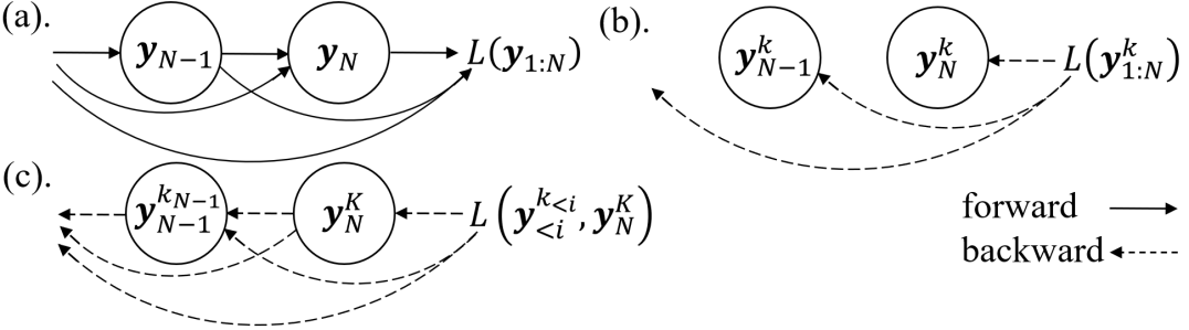
Figure 1: (a). The forward pass of NVC. (b). The backward pass of Naïve implementation (Alg. 1). (c). The backward pass of advanced implementation (Alg. 3).

Incomplete Total Derivative Evaluation According to the latent’s autogressive dependency in Eq. 1 and target $\mathcal{L}$ in Eq. 12, we draw the computational graph to describe the latent dependency as Fig. 1.(a) and expand the total derivative $d\mathcal{L}/d\bm{y}_{i}$:

$$\frac{d\mathcal{L}(\bm{y}_{1:N})}{d\bm{y}_{i}}= \sum_{j=i}^{N}(\underbrace{\sum_{l=i+1}^{j}\frac{\partial\bm{y}_{l}}{\partial\bm{y}_{i}}\frac{d\mathcal{L}_{j}(\bm{y}_{1:j})}{d\bm{y}_{l}}}_{\textrm{ignored by na\"{i}ve implementation}}+\frac{\partial\mathcal{L}_{j}(\bm{y}_{1:j})}{\partial\bm{y}_{i}}).$$ (17)

As shown in Eq. 16 and Alg. 1, The naïve implementation treats the total derivative $d\mathcal{L}/d\bm{y}_{i}$ as the sum of the frame level partial derivative $\partial\mathcal{L}_{j}/\partial\bm{y}_{i}$, which is the direct contribution of frame $i^{th}$ latent $\bm{y}_{i}$ to $j^{th}$ frame’s R-D cost $\mathcal{L}_{j}$ (as marked in Eq. 17). This incomplete evaluation of gradient signal brings sub-optimality.

Incorrect Value to Evaluate Gradient Besides the incomplete gradient issue, Alg. 1 simultaneously updates all the posterior parameter $\bm{y}_{1:N}$ with gradient evaluated at the same step $\bm{y}_{1:N}^{k}$. However, to evaluate the gradient of $\bm{y}_{i}$, all its descendant latent $\bm{y}_{>i}$ should already complete all $K$ steps of gradient ascent. Moreover, once $\bm{y}_{i}$ is updated, all its descendant latent $\bm{y}_{>i}$ should be re-initialized by FAVI. Specifically, the correct value to evaluate the gradient is:

$$\bm{y}^{k_{i}+1}_{i}\leftarrow\bm{y}^{k_{i}}_{i}+\alpha\frac{d\mathcal{L}(\bm{y}_{1}^{k_{1}},...,\bm{y}_{i}^{k_{i}},\bm{y}^{K}_{>i})}{d\bm{y}^{k_{i}}_{i}},$$

$$\textrm{where }\bm{y}_{>i}^{0}=f_{\phi}(\bm{x},\bm{y}_{1}^{k_{1}},...,\bm{y}_{i}^{k_{i}}),$$ (18)

where $\bm{y}_{i}^{k_{i}}$ denotes the latent $\bm{y}_{i}$ after $k_{i}$ steps of update. In next section, we show how to correct both of the above-mentioned issues by recursively applying back-propagating through gradient ascent (Domke, 2012).

3.4 An Accurate Implementation

Accurate SAVI on 2-level non-factorized latent We first extend the original SAVI on 1-level latent (Kim et al., 2018) to 2-level non-factorized latent. As the notation in NVC, we denote $\bm{x}$ as evidence, $\bm{y}_{1}$ as the variational posterior parameter of the first level latent $\bm{\tilde{y}}_{1}$, $\bm{y}_{2}$ as the variational posterior parameter of the second level latent $\bm{\tilde{y}}_{2}$, and the ELBO to maximize as $\mathcal{L}(\bm{y}_{1},\bm{y}_{2})$. The posterior $q(\bm{\tilde{y}}_{1},\bm{\tilde{y}}_{2}|\bm{x})$ factorizes as $q(\bm{\tilde{y}}_{1}|\bm{x})q(\bm{\tilde{y}}_{2}|\bm{\tilde{y}}_{1},\bm{x})$, which means that $\bm{y}_{2}$ depends on $\bm{y}_{1}$. Given $\bm{y}_{1}$ is fixed, we can directly optimize $\bm{y}_{2}$ by gradient ascent. However, it requires some tricks to optimize $\bm{y}_{1}$. The intuition is, we do not want to find a $\bm{y}_{1}$ that maximizes $\mathcal{L}(\bm{y}_{1},\bm{y}_{2})$ given a fixed $\bm{y}_{2}$. Instead, we want to find a $\bm{y}_{1}$, whose $\max_{\bm{y}_{2}}\mathcal{L}(\bm{y}_{1},\bm{y}_{2})$ is maximum. This translates to the optimization problem as:

$$\bm{y}_{1}\leftarrow\arg\max_{\bm{y}_{1}}\mathcal{L}(\bm{y}_{1},\bm{y}_{2}^{*}(\bm{y}_{1})),$$

$$\textrm{ where }\bm{y}_{2}^{*}(\bm{y}_{1})\leftarrow\arg\max_{\bm{y}_{2}}\mathcal{L}(\bm{y}_{1},\bm{y}_{2}).$$ (19)

In fact, Eq. 19 is a variant of setup in back-propagating through gradient ascent (Samuel & Tappen, 2009; Domke, 2012). The difference is, our $\bm{y}_{1}$ also contributes directly to optimization target $\mathcal{L}(\bm{y}_{1},\bm{y}_{2})$. From this perspective, Eq. 19 is also closely connected to Kim et al. (2018), if we treat $\bm{y}_{1}$ as the amortized encoder parameter and $\bm{y}_{2}$ as latent.

And as SAVI on 1-level latent (Kim et al., 2018), we need to solve Eq. 19 using gradient ascent. Specifically, denote $\alpha$ as learning rate, $K$ as the total gradient ascent steps, $\bm{y}_{1}^{k_{1}}$ as the $\bm{y}_{1}$ after $k_{1}$ step update, $\bm{y}_{2}^{k_{2}}$ as the $\bm{y}_{2}$ after $k_{2}$ step update, and $f(.)$ as FAVI initialing posterior parameters $\bm{y}_{1}^{0},\bm{y}_{2}^{0}$, the optimization problem as Eq. 19 translates into the update rule as:

$$\bm{y}_{1}^{k_{1}+1}\leftarrow\bm{y}_{1}^{k_{1}}+\alpha\frac{d\mathcal{L}(\bm{y}_{1}^{k_{1}},\bm{y}_{2}^{K})}{d\bm{y}_{1}^{k_{1}}},$$

$$\bm{y}_{2}^{k_{2}+1}\leftarrow\bm{y}_{2}^{k_{2}}+\alpha\frac{d\mathcal{L}(\bm{y}_{1}^{k_{1}},\bm{y}_{2}^{k_{2}})}{d\bm{y}_{2}^{k_{2}}}\textrm{, where }\bm{y}_{2}^{0}=f(\bm{x},\bm{y}_{1}^{k_{1}}).$$ (20)

To solve Eq. 20, we note that although $d\mathcal{L}(\bm{y}_{1}^{k_{1}},\bm{y}_{2}^{k_{2}})/d\bm{y}_{2}^{k_{2}}$ can be directly computed, $d\mathcal{L}(\bm{y}_{1}^{k_{1}},\bm{y}_{2}^{K})/d\bm{y}_{1}^{k_{1}}$ is not straightforward. Let’s consider a simple example when the gradient ascent step $K=1$:

• First, we initialize $\bm{y}_{1},\bm{y}_{2}$ by FAVI $\bm{y}_{1}^{0}\leftarrow\textrm{FAVI}(\bm{x}),\bm{y}_{2}^{0}\leftarrow\textrm{FAVI}(\bm{x},\bm{y}_{1}^{0})$.

• Next, we optimize $\bm{y}_{2}$ by one step gradient ascent as $\bm{y}_{2}^{1}\leftarrow\bm{y}_{2}^{0}+\alpha d\mathcal{L}(\bm{y}_{2}^{0},\bm{y}_{1}^{0})/d\bm{y}_{2}^{0}$ and evaluate ELBO as $\mathcal{L}(\bm{y}_{1}^{0},\bm{y}_{2}^{1})$.

• Next, we optimize $\bm{y}_{1}$ to maximize $\mathcal{L}(\bm{y}_{1}^{0},\bm{y}_{2}^{1})$, and the gradient is

  $$\frac{d\mathcal{L}(\bm{y}_{1}^{0},\bm{y}_{2}^{1})}{d\bm{y}_{1}}=\frac{\partial\mathcal{L}(\bm{y}_{1}^{0},\bm{y}_{2}^{1})}{\partial\bm{y}_{1}^{0}}+\frac{\partial\bm{y}_{2}^{0}}{\partial\bm{y}_{1}^{0}}\frac{d\mathcal{L}(\bm{y}_{1}^{0},\bm{y}_{2}^{1})}{d\bm{y}_{2}^{0}}.$$

  With FAVI relationship, we naturally have $\partial\bm{y}_{2}^{0}/\partial\bm{y}_{1}^{0}$. And we need to evaluate is $d\mathcal{L}(\bm{y}_{1}^{0},\bm{y}_{2}^{1})/d\bm{y}_{2}^{0}$. And this is where back-prop through gradient ascent (Samuel & Tappen, 2009; Domke, 2012) works:

  $$\frac{d\mathcal{L}(\bm{y}_{1}^{0},\bm{y}_{2}^{1})}{d\bm{y}_{2}^{0}} =\frac{\partial\bm{y}_{2}^{1}}{\partial\bm{y}_{2}^{0}}\frac{d\mathcal{L}(\bm{y}_{1}^{0},\bm{y}_{2}^{1})}{d\bm{y}_{2}^{1}}$$

  $$=(I+\alpha\frac{\partial^{2}\mathcal{L}(\bm{y}_{2}^{0},\bm{y}_{1}^{0})}{\partial^{2}\bm{y}^{0}_{2}})\frac{d\mathcal{L}(\bm{y}_{1}^{0},\bm{y}_{2}^{1})}{d\bm{y}_{2}^{1}}.$$

  Again, $d\mathcal{L}(\bm{y}_{1}^{0},\bm{y}_{2}^{1})/d\bm{y}_{2}^{1}$ is known.

• By now, we have collect all parts to solve $d\mathcal{L}(\bm{y}_{1}^{0},\bm{y}_{2}^{1})/d\bm{y}_{1}^{0}$. And we can finally update $\bm{y}_{1}^{0}$ as $\bm{y}_{1}^{1}\leftarrow\bm{y}_{1}^{0}+\alpha d\mathcal{L}(\bm{y}_{1}^{0},\bm{y}_{2}^{1})/d\bm{y}_{1}^{0}$.

For $K>1$, we can extend the example and implement Eq. 20 as Alg. 2. Specifically, we first initialize $\bm{y}_{1}^{0}$ from FAVI. Then we conduct gradient ascent on $\bm{y}_{1}$ with gradient $d\mathcal{L}(\bm{y}_{1}^{k_{1}},\bm{y}_{2}^{K})/d\bm{y}_{1}^{k_{1}}$ computed from the procedure grad-2-level($\bm{x},\bm{y}_{1}^{k_{1}}$). And each time grad-2-level($\bm{x},\bm{y}_{1}^{k_{1}}$) is evaluated, $\bm{y}_{2}$ goes through a re-initialization and $K$ steps of gradient ascent. The above procedure corresponds to Eq. 20. The key of Alg. 2 is the evaluation of gradient $d\mathcal{L}(\bm{a}^{k},\bm{b}^{K})/d\bm{a}^{k}$. Formally, we have:

Theorem 3.3.

After grad-2-level($\bm{x},\bm{y}_{1}^{k_{1}}$) of Alg. 2 executes, we have the return value $d\mathcal{L}(\bm{y}_{1}^{k_{1}},\bm{y}_{2}^{K})/d\bm{y}_{1}^{k_{1}}=\overleftarrow{\bm{y}_{1}}$. (See proof in Appendix. B)

Algorithm 2 Proposed Accurate SAVI on 2-level Latent

  procedure solve-2-level($\bm{x}$)

  initialize $\bm{y}_{1}^{0}\leftarrow f_{\phi}(\bm{x})$ from FAVI.

  for $k_{1}=0$ to $K-1$ do

     $\frac{d\mathcal{L}(\bm{y}_{1}^{k_{1}},\bm{y}_{2}^{K})}{d\bm{y}_{1}^{k_{1}}}=\textrm{grad-2-level}(\bm{x},\bm{y}_{1}^{k_{1}})$

     $\bm{y}_{1}^{k_{1}+1}\leftarrow\bm{y}_{1}^{k_{1}}+\alpha\frac{d\mathcal{L}(\bm{y}_{1}^{k_{1}},\bm{y}_{2}^{K})}{d\bm{y}_{1}^{k_{1}}}$

  end for

  return $\bm{y}_{1}^{K},\bm{y}_{2}^{K}$

  

  procedure grad-2-level($\bm{x},\bm{y}_{1}^{k_{1}}$)

  initialize $\bm{y}_{2}^{0}\leftarrow f_{\phi}(\bm{x},\bm{y}_{1}^{k_{1}})$ from FAVI.

  for $k_{2}=0$ to $K-1$ do

     $\bm{y}_{2}^{k_{2}+1}\leftarrow\bm{y}_{2}^{k_{2}}+\alpha\frac{d\mathcal{L}(\bm{y}_{1}^{k_{1}},\bm{y}_{2}^{k_{2}})}{d\bm{y}_{2}^{k_{2}}}$

  end for

  initialize $\overleftarrow{\bm{y}_{1}}\leftarrow\frac{\partial\mathcal{L}(\bm{y}_{1}^{k_{1}},\bm{y}_{2}^{K})}{\partial\bm{y}_{1}^{k_{1}}}$, $\overleftarrow{\bm{y}_{2}}^{K}\leftarrow\frac{d\mathcal{L}(\bm{y}_{1}^{k_{1}},\bm{y}_{2}^{K})}{d\bm{y}_{2}^{K}}$

  for $k_{2}=K-1$ to $0$ do

     $\overleftarrow{\bm{y}_{1}}\leftarrow\overleftarrow{\bm{y}_{1}}+\alpha\frac{\partial^{2}\mathcal{L}(\bm{y}_{1}^{k_{1}},\bm{y}_{2}^{k_{2}})}{\partial\bm{y}_{1}^{k_{1}}\partial\bm{y}_{2}^{k_{2}}}\overleftarrow{\bm{y}_{2}}^{k_{2}+1}$

     $\overleftarrow{\bm{y}_{2}}^{k_{2}}\leftarrow\overleftarrow{\bm{y}_{2}}^{k_{2}}+\alpha\frac{\partial^{2}\mathcal{L}(\bm{y}_{1}^{k_{1}},\bm{y}_{2}^{k_{2}})}{\partial\bm{y}_{2}^{k_{2}}\partial\bm{y}_{2}^{k_{2}}}\overleftarrow{\bm{y}_{2}}^{k_{2}+1}$

  end for

  $\overleftarrow{\bm{y}_{1}}=\overleftarrow{\bm{y}_{1}}+\frac{\partial\bm{y}_{2}^{0}}{\partial\bm{y}_{1}^{k_{1}}}\overleftarrow{\bm{y}_{2}}^{0}$

  return $\frac{d\mathcal{L}(\bm{y}_{1}^{k_{1}},\bm{y}_{2}^{K})}{d\bm{y}_{1}^{k_{1}}}=\overleftarrow{\bm{y}_{1}}$

Accurate SAVI on DAG Latent Then, we extend the result on 2-level latent to general non-factorized latent with dependency described by DAG. This DAG is the computational graph during network inference, and it is also the directed graphical model (DGM) (Koller & Friedman, 2009) defining the factorization of latent variables during inference. This extension is necessary for SAVI on latent with complicated dependency (e.g. bit allocation of NVC).

Similar to the 2-level latent setup, we consider performing SAVI on $N$ variational posterior parameter $\bm{y}_{1},...,\bm{y}_{N}$ with their dependency defined by a computational graph $\mathcal{G}$, i.e., their corresponding latent variable $\bm{\tilde{y}}_{1},...,\bm{\tilde{y}}_{N}$’s posterior distribution factorizes as $\mathcal{G}$. Specifically, we denote $\bm{y}_{j}\in\mathcal{C}(\bm{y}_{i}),\bm{y}_{i}\in\mathcal{P}(\bm{a}_{j})$ if an edge exists from $\bm{y}_{i}$ to $\bm{y}_{j}$. This indicates that $\bm{\tilde{y}}_{j}$ conditions on $\bm{\tilde{y}}_{i}$. Without loss of generality, we assume $\bm{y}_{1},...,\bm{y}_{N}$ is sorted in topological order. This means that if $\bm{y}_{j}\in\mathcal{C}(\bm{y}_{i}),\bm{y}_{i}\in\mathcal{P}(\bm{y}_{j})$, then $i<j$. Each latent is optimized by $K$-step gradient ascent, and $\bm{y}_{i}^{k_{i}}$ denotes the latent $\bm{y}_{i}$ after $k_{i}$ steps of update. Then, similar to 2-level latent, we can solve this problem by recursively applying back-propagating through gradient ascent (Samuel & Tappen, 2009; Domke, 2012) to obtain Alg. 3.

Specifically, we add a fake latent $\bm{y}_{0}$ to the front of all $\bm{y}$s. Its children are all the $\bm{y}$s with 0 in-degree. Then, we can solve the SAVI on $\bm{y}_{1},...,\bm{y}_{N}$ using gradient ascent by executing the procedure grad-dag($\bm{x},\bm{y}_{0}^{k_{0}},...,\bm{y}_{i}^{k_{i}}$) in Alg. 3 recursively. Inside procedure grad-dag($\bm{x},\bm{y}_{0}^{k_{0}},...,\bm{y}_{i}^{k_{i}}$), the gradient to update $\bm{y}_{i}$ relies on the convergence of its children $\bm{y}_{j}\in\mathcal{C}(\bm{y}_{i})$, which is implemented by the recursive depth-first search (DFS) in line 11. And upon the completion of procedure grad-dag($\bm{x},\bm{y}_{0}^{0}$), all the latent converges to $\bm{y}_{1}^{K},...,\bm{y}_{N}^{K}$. Similar to the 2-level latent case, the key of Alg. 3 is the evaluation of gradient $d\mathcal{L}(\bm{y}_{0}^{k_{0}},...,\bm{y}_{i}^{k_{i}},\bm{y}_{>i}^{K})/d\bm{y}_{i}^{k_{i}}$. Formally, we have:

Theorem 3.4.

After the procedure grad-dag($\bm{x},\bm{y}_{0}^{k_{0}},...,\bm{y}_{i}^{k_{i}}$) in Alg. 3 executes, we have the return value $d\mathcal{L}(\bm{y}_{0}^{k_{0}},...,\bm{y}_{i}^{k_{i}},\bm{y}_{>i}^{K})/d\bm{y}_{i}^{k_{i}}=\overleftarrow{\bm{y}_{i}}$. (See proof in Appendix. B.)

Algorithm 3 Proposed Accurate SAVI on DAG Latent

  procedure solve-dag($\bm{x}$)

  for $\bm{y}_{j}$ with parent $\mathcal{P}(\bm{y}_{j})=\varnothing$ do

     add $\bm{y}_{j}$ to fake node $\bm{y}_{0}$’s children $\mathcal{C}(\bm{y}_{0})$

  end for

  grad-dag($\bm{x},\bm{y}_{0}^{0}$)

  return $\bm{y}_{1}^{K},...,\bm{y}_{N}^{K}$

  

  procedure grad-dag($\bm{x},\bm{y}_{0}^{k_{0}},...,\bm{y}_{i}^{k_{i}}$)

  for $\bm{y}_{j}\in\mathcal{C}(\bm{y}_{i})$ in topological order do

     initialize $\bm{y}_{j}^{0}\leftarrow f(\bm{x},\bm{y}_{0}^{k_{0}},...,\bm{y}_{<j}^{k_{<j}})$ from SAVI

     for $k_{j}=0,...,K-1$ do

        $\frac{d\mathcal{L}(\bm{y}_{0}^{k_{0}},...,\bm{y}_{j}^{k_{j}},\bm{y}_{>j}^{K})}{d\bm{y}_{j}^{k_{j}}}\leftarrow\textrm{grad-dag}(\bm{x},\bm{y}_{0}^{k_{0}},...,\bm{y}_{j}^{k_{j}})$

        $\bm{y}_{j}^{k_{j}+1}\leftarrow\bm{y}_{j}^{k_{j}}+\alpha\frac{d\mathcal{L}(\bm{y}_{0}^{k_{0}},...,\bm{y}_{j}^{k_{j}},\bm{y}_{>j}^{K})}{d\bm{y}_{j}^{k_{j}}}$

     end for

  end for

  $\overleftarrow{\bm{y}_{i}}\leftarrow\frac{\partial\mathcal{L}(\bm{y}_{0}^{k_{0}},...,\bm{y}_{i}^{k_{i}},\bm{y}_{>i}^{K})}{\partial\bm{y}_{i}^{k_{i}}}$

  for $\bm{y}_{j}\in\mathcal{C}(\bm{y}_{i})$ in topological order do

     $\overleftarrow{\bm{y}_{j}}^{K}\leftarrow\frac{d\mathcal{L}(\bm{y}_{0}^{k_{0}},...,\bm{y}_{i}^{k_{i}},\bm{y}_{>i}^{K})}{d\bm{y}_{j}^{K}}$

     for $k_{j}=K-1,...,0$ do

        $\overleftarrow{\bm{y}_{i}}\leftarrow\overleftarrow{\bm{y}_{i}}+\alpha\frac{\partial^{2}\mathcal{L}(\bm{y}_{0}^{k_{0}},...,\bm{y}_{j}^{k_{j}},\bm{y}_{>j}^{K})}{\partial\bm{y}_{i}^{k_{i}}\partial\bm{y}_{j}^{k_{j}}}\overleftarrow{\bm{y}_{j}}^{k_{j}+1}$

        $\overleftarrow{\bm{y}_{j}}^{k_{j}}\leftarrow\overleftarrow{\bm{y}_{j}}^{k_{j}+1}+\alpha\frac{\partial^{2}\mathcal{L}(\bm{y}_{0}^{k_{0}},...,\bm{y}_{j}^{k_{j}},\bm{y}_{>j}^{K})}{\partial\bm{y}_{j}^{k_{j}}\partial\bm{y}_{j}^{k_{j}}}\overleftarrow{\bm{y}_{j}}^{k_{j}+1}$

     end for

     $\overleftarrow{\bm{y}_{i}}\leftarrow\overleftarrow{\bm{y}_{i}}+\frac{\partial\bm{y}_{j}^{0}}{\partial\bm{y}_{i}^{k_{i}}}\overleftarrow{\bm{y}_{j}}^{0}$

  end for

  return $\frac{d\mathcal{L}(\bm{y}_{0}^{k_{0}},...,\bm{y}_{i}^{k_{i}},\bm{y}_{>i}^{K})}{d\bm{y}_{i}^{k_{i}}}=\overleftarrow{\bm{y}_{i}}$

4 Complexity Reduction

An evident problem of the accurate SAVI (Sec. 3.4) is the temporal complexity. Given the frame number $N$ and gradient ascent step $K$, Alg. 3 has temporal complexity of $\Theta(K^{N})$. NVC with GoP size $10$ has approximately $N=20$ latent, and the SAVI on neural image compression (Yang et al., 2020b; Gao et al., 2022) takes around $K=2000$ step to converge. For bit allocation, the complexity of Alg. 3 is $\approx 2000^{20}$, which is intractable.

4.1 Temporal Complexity Reduction

Therefore, we provide an approximation to the SAVI on DAG. The general idea is that, the SAVI on DAG (Alg. 3) satisfies both requirement on gradient signal described in Sec. 3.3. We can not make it tractable without breaking them. Thus, we break one of them for tractable complexity, while maintaining good performance. Specifically, We consider the approximation as:

$$\frac{d\mathcal{L}(\bm{y}_{0}^{k_{0}},...,\bm{y}_{i}^{k_{i}},\bm{y}_{>i}^{K})}{d\bm{y}_{i}^{k_{i}}}\approx\frac{d\mathcal{L}(\bm{y}_{0}^{k_{0}},...,\bm{y}_{i}^{k_{i}},\bm{y}_{>i}^{0})}{d\bm{y}_{i}^{k_{i}}},$$ (21)

which obeys the requirement 1 in Sec. 3.3 while breaks the requirement 2. Based on Eq. 21, we design an approximation of SAVI on DAG. Specifically, with the approximation in Eq. 21, the recurrent gradient computation in Alg. 3 becomes unnecessary as the right hand side of Eq. 21 does not require $\bm{y}_{>i}^{K}$. However, to maintain the dependency of latent, we still need to ensure that the children node $\bm{y}_{j}\in\mathcal{C}(\bm{y}_{i})$ are re-initialized by FAVI every-time when $\bm{y}_{i}$ is updated. Therefore, we traverse the graph in topological order, keep the children node $\bm{y}_{j}$ untouched until all its parent node $\bm{y}_{i}\in\mathcal{P}(\bm{y}_{j})$’s gradient ascent is completed. And the resulting approximate SAVI is Alg. 4. Its temporal complexity is $\Theta(KN)$.

Algorithm 4 Proposed Approximated SAVI

  procedure solve-approx($\bm{x}$)

  for $i=1$ to $N$ do

     initialize $\bm{y}_{i}^{0},...,\bm{y}_{N}^{0}\leftarrow f_{\phi}(\bm{x},\bm{y}_{<i}^{K})$ from FAVI.

     for $k=0$ to $K-1$ do

        $\frac{d\mathcal{L}(\bm{y}_{<i}^{K},\bm{y}_{i}^{k},\bm{y}_{>i}^{K})}{d\bm{y}_{i}^{k}}\approx\frac{d\mathcal{L}(\bm{y}_{<i}^{K},\bm{y}_{i}^{k},\bm{y}_{>i}^{0})}{d\bm{y}_{i}^{k}}$

        $\bm{y}_{i}^{k+1}\leftarrow\bm{y}_{i}^{k}+\alpha\frac{d\mathcal{L}(\bm{y}_{<i}^{K},\bm{y}_{i}^{k},\bm{y}_{>i}^{K})}{d\bm{y}_{i}^{k}}$

     end for

  end for

  return $\bm{y}_{1}^{K},...,\bm{y}_{N}^{K}$

4.2 Spatial Complexity Reduction

Despite the the approximated SAVI on DAG reduce the temporal complexity from $\Theta(K^{N})$ to $\Theta(KN)$, the spatial complexity remains $\Theta(N)$. Though most of NVC approaches adopt a small GoP size of 10-12 (Lu et al., 2019; Li et al., 2021), there are emerging approach extending GoP size to 100 (Hu et al., 2022). Therefore, it is important to reduce the spatial complexity to constant for scalability.

Specifically, our approximated SAVI on DAG uses the gradient of GoP-level likelihood $\mathcal{L}$, which takes $\Theta(N)$ memory. We empirically find that we can reduce the likelihood range for gradient evaluation from the whole GoP to $C$ future frames:

$$\frac{d\mathcal{L}}{d\bm{y}_{i}^{k_{i}}}=\sum_{j=i}^{N}\frac{d\mathcal{L}_{j}}{d\bm{y}_{i}^{k_{i}}}\approx\sum_{j=i}^{min(i+C,N)}\frac{d\mathcal{L}_{j}}{d\bm{y}_{i}^{k_{i}}},$$ (22)

where $C$ is a constant. Then, the spatial complexity is reduced to $\Theta(C)$, which is constant to GoP size $N$.

5 Experimental Results

	BD-BR (%) $\downarrow$					BD-PSNR (dB) $\uparrow$
Method	Class B	Class C	Class D	Class E	UVG	Class B	Class C	Class D	Class E	UVG
DVC (Lu et al., 2019) as Baseline
Li et al. (2016)∗	20.21	17.13	13.71	10.32	16.69	-0.54	-	-	-0.32	-0.47
Li et al. (2022b)∗	-6.80	-2.96	0.48	-6.85	-4.12	0.19	-	-	0.28	0.14
OEU (Lu et al., 2020a)	-13.57	-11.29	-18.97	-12.43	-13.78	0.39	0.49	0.83	0.48	0.48
Proposed-Scalable (Sec. 4.2)	-21.66	-26.44	-29.81	-22.78	-22.86	0.66	1.10	1.30	0.91	0.79
Proposed-Approx (Sec. 4.1)	-32.10	-31.71	-35.86	-32.93	-30.92	1.03	1.38	1.67	1.41	1.15
DCVC (Li et al., 2021) as Baseline
OEU (Lu et al., 2020a)	-10.75	-14.34	-16.30	-7.15	-16.07	0.30	0.58	0.74	0.29	0.50
Proposed-Scalable (Sec. 4.2)	-24.67	-24.71	-24.71	-30.35	-29.68	0.65	0.95	1.12	1.15	0.83
Proposed-Approx (Sec. 4.1)	-32.89	-33.10	-32.01	-36.88	-39.66	0.91	1.37	1.55	1.58	1.18
HSTEM (Li et al., 2022a) as Baseline
Proposed-Scalable (Sec. 4.2)	-15.42	-17.21	-19.95	-10.03	-3.18	0.32	0.58	0.81	0.26	0.07

Table 1: The BD-BR and BD-PSNR of our approach compared with baselines (w/o bit allocation) and other bit allocation approaches. ^∗ The data comes from Li et al. (2022b). We mark some data with ‘-’ as they are not reported by Li et al. (2022b).

5.1 Evaluation on Density Estimation

As the proposed SAVI without approximation (Proposed-Accurate, Sec. 3.4) is intractable for NVC, we evaluate it on small density estimation tasks. Specifically, we consider a 2-level VAE with inference model $\bm{x}\rightarrow\bm{\tilde{y}}_{1}\rightarrow\bm{\tilde{y}}_{2}$, where $\bm{x}$ is observed data, $\bm{\tilde{y}}_{1}$ is the first level latent with dimension 100 and $\bm{\tilde{y}}_{2}$ is the second level latent with dimension 50. We adopt the same 2-level VAE architecture as Burda et al. (2015). And the dataset we use is MNIST (LeCun et al., 1998). More details are provided in Appendix. C.

	NLL	t-test p-value
FAVI (2-level VAE)	$\leq$ 98.3113	-
Original SAVI	$\leq$ 91.5530	$\leq$ 0.001 (w/ FAVI)
Proposed-Approx (Sec. 4.1)	$\leq$ 91.5486	$\leq$ 0.001 (w/ Original)
Proposed-Accurate (Sec. 3.4)	$\leq$ 91.5482	$\leq$ 0.001 (w/ Approx)

Table 2: The NLL result on density estimation.

We evaluate the negative log likelihood (NLL) lowerbound of FAVI, Original SAVI (Alg.1), proposed SAVI without approximation (Proposed-Accurate, Sec. 3.4) and proposed SAVI with approximation (Proposed-Approx, Sec. 4.1). Tab. 2 shows that our Proposed-Accurate achieves a lower NLL ($\leq 91.5482$) than original SAVI ($\leq 91.5530$). And our Proposed-Approx ($\leq 91.5486$) is only marginally outperformed by Proposed-Accurate, which indicates that this approximation does not harm performance significantly. As the mean NLL difference between Proposed-Accurate and Proposed-Approx is small, we additionally perform pair-wise t-test between methods and report p-values. And the results suggest that the difference between methods is significant ($p\leq 0.001$).

5.2 Evaluation on Bit Allocation

Experiment Setup We evaluate our bit allocation method based on 3 NVC baselines: DVC (Lu et al., 2019), DCVC (Li et al., 2021) and HSTEM (Li et al., 2022a). For all 3 baseline methods, we adopt the official pre-trained models. As DVC and DCVC do not provide I frame model, we adopt Cheng et al. (2020) with pre-trained models provided by Bégaint et al. (2020). Following baselines, we adopt HEVC Common Testing Condition (CTC) (Bossen et al., 2013) and UVG dataset (Mercat et al., 2020). And the GoP size is set to 10 for HEVC CTC and 12 for UVG dataset. The R-D performance is measured by Bjontegaard-Bitrate (BD-BR) and BD-PSNR (Bjontegaard, 2001). For the proposed approach, we evaluate the approximated SAVI (Alg. 4) and its scalable version with $C=2$. We adopt Adam (Kingma & Ba, 2014) optimizer with $lr=1\times 10^{-3}$ to optimize $\bm{y}_{1:N}$ for $K=2000$ iterations. For other bit allocation methods, we select a traditional $\lambda$-domain approach (Li et al., 2016), a recent $\lambda$-domain approach (Li et al., 2020) and online encoder update (OEU) (Lu et al., 2020a). More details are presented in Appendix. C.

Main Results We extensively evaluate the R-D performance of proposed SAVI with approximation (Proposed-Approx, Sec. 4.1) and proposed SAVI with scalable approximation (Proposed-Scalable, Sec. 4.2) on 3 baselines and 5 datasets. As Tab. 1 shows, for DVC (Lu et al., 2019) and DCVC (Li et al., 2021), our Proposed-Approx and Proposed-Scalable outperform all other bit allocation methods by large margin. It shows that the current best bit allocation method, OEU (Lu et al., 2020a), still has a room of $0.5$ dB BD-PSNR to improve compared with our result. For HSTEM (Li et al., 2022a) with large model, we only evaluate our Proposed-Scalable. As neither OEU (Lu et al., 2020a) nor Proposed-Approx is able to run on HSTEM within 80G RAM limit. Moreover, as HSTEM has a bit allocation module, the effect of bit allocation is not as evident as DVC and DCVC. However, our bit allocation still brings a significant improvement of more than $0.4$ dB PSNR over HSTEM.

	BD-BR (%)	Enc Time (s)	RAM (GB)
DVC (Lu et al., 2019) as Baseline
Baseline	-	$\leq$1.0	1.02
Li et al. (2016)	13.71	$\leq$1.0	1.02
Li et al. (2022b)	0.48	$\leq$1.0	1.02
OEU (Lu et al., 2020a)	-18.97	15.2	5.83
Original SAVI	-14.76	158.5	3.05
Original SAVI (per-frame)	-20.12	55.3	2.94
Proposed-Scalable (Sec. 4.2)	-29.81	74.6	2.12
Proposed-Approx (Sec. 4.1)	-35.86	528.3	5.46
VTM 13.2	-	219.9	1.40

Table 3: The R-D performance and the encoder resource consumption of different approaches. Encode time is per-frame and measured with AMD EPYC 7742 CPU and Nvidia A100 GPU.

	steps, lr	BD-BR (%)	Enc Time (s)
Proposed-Scalable (Sec. 4.2)	2000, $1\times 10^{-3}$	-29.81	74.6
	1000, $2\times 10^{-3}$	-25.37	37.3
	500, $4\times 10^{-3}$	-18.99	18.6
Proposed-Approx (Sec. 4.1)	2000, $1\times 10^{-3}$	-35.86	528.3
	1000, $2\times 10^{-3}$	-31.21	264.1
	500, $4\times 10^{-3}$	-25.60	132.0

Table 4: The R-D performance and the encoding time consumption of different gradient ascent step and learning rate. We assume that the temporal complexity is approximately linear to steps.

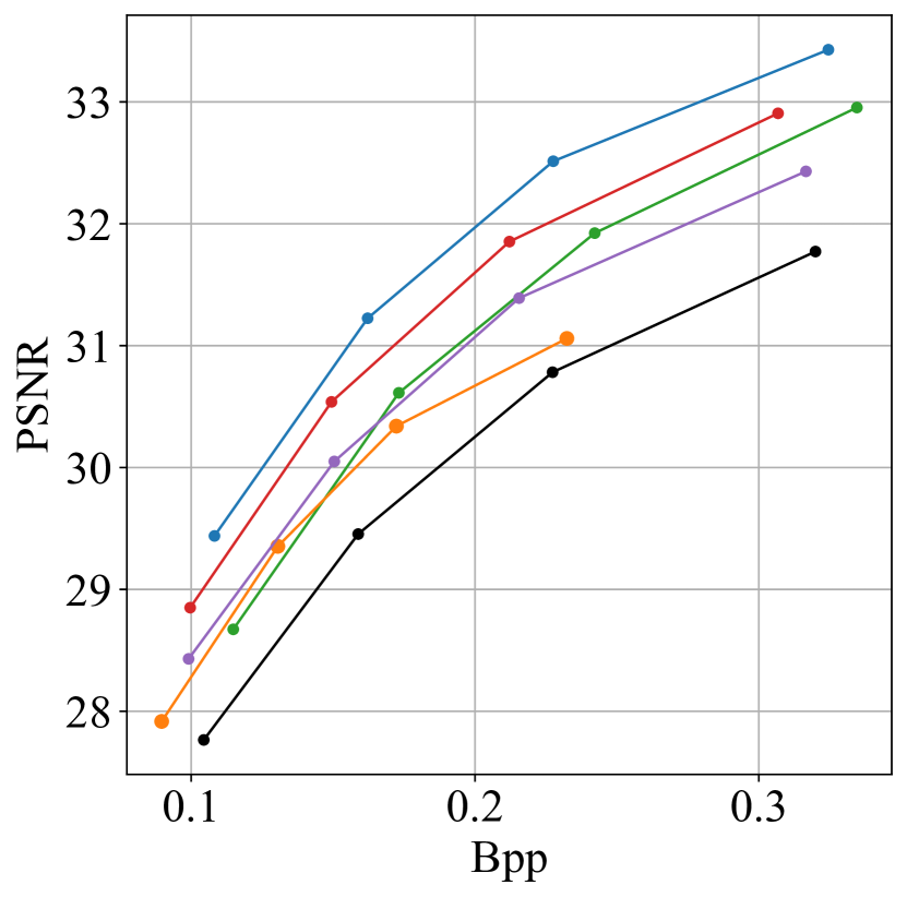
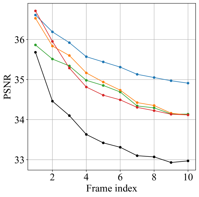
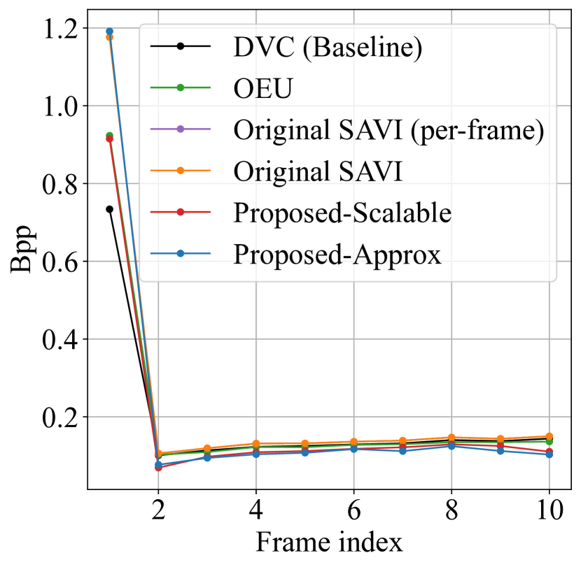
Figure 2: upper-left. The R-D performance of different methods. upper-right. The RAM-GoP size relationship of different methods. lower-left. The PSNR-frame index relationship before and after bit allocation. lower-right. The bpp-frame index relationship before and after bit allocation.

Ablation Study We evaluate the R-D performance, encoding time and memory consumption of different methods with DVC (Lu et al., 2019) on HEVC Class D. As Tab. 3 and Fig. 2.upper-left show, the Proposed-Approx (-35.86%) significantly outperforms the original SAVI (-14.76%) in terms of BD-BR. Furthermore, it significantly outperforms all other bit allocation approaches. On the other hand, our Proposed-Scalable effectively decreases encoding time (from 528.3s to 74.6s). However, its R-D performance (-29.81%) remains superior than all other bit allocation approaches by large margin. On the other hand, SAVI based approaches improve R-D performance not only by bit allocation, but also by reducing the amortization gap and discretization gap (Yang et al., 2020b). To investigate the net improvement by bit allocation, we perform (Yang et al., 2020b) in a per-frame manner. And the resulting method (Original SAVI (per-frame)) improves the R-D performance by $20\%$. This means that the net enhancement brought by bit allocation is around $15\%$. Furthermore, as shown in Fig. 2.upper-right, the memory requirement of our Proposed-Scalable is constant to GoP size. While for OEU (Lu et al., 2020a), original SAVI and Proposed-Approx, the RAM is linear to GoP size. Despite the encoding time and RAM of our approach is higher than baseline, the decoding remains the same. Furthermore, compared with other encoder for R-D performance benchmark purpose (VTM 13.2), the encoding time and memory of our approach is reasonable.

For both Proposed-Approx and Proposed-Scalable, it is possible to achieve speed-performance trade-off by adjusting gradient ascent steps and learning. In Tab. 4, we can see that reducing number of gradient ascent steps linearly reduce the encoding time while maintain competitive R-D performance. Specifically, Proposed-Scalable with $500$ steps and $1\times 10^{-3}$ lr achieves similar BD-BR (-18.99 vs -18.97%) and encoding time (18.6 vs 15.2s) as OEU (Lu et al., 2020a), with less than half RAM requirement (2.12 vs 5.83GB).

Analysis To better understand our bit allocation methods, we show the per-frame bpp and PSNR before and after bit allocation in Fig. 2.lower-left and Fig. 2.lower-right. It can be seen that the frame quality of baseline method drops rapidly during encoding process (from $35.5$ to $33.0$ dB), while our proposed bit allocation approach alleviate this degradation (from $36.5$ to $35.0$ dB). On the other hand, all bit allocation methods allocates more bitrate to I frame. The original SAVI need more bitrate to achieve the same frame quality as the proposed approach, that is why its R-D performance is inferior.

Qualitative Results See Appendix. D.

6 Related Works

Bit Allocation for Neural Video Compression Rippel et al. (2019); Li et al. (2022b) are the pioneer of bit allocation for NVC, who reuse the empirical model from traditional codec. More recently, Li et al. (2022a) propose a feed-forward bit allocation approach with quantization step-size predicted by neural network. Other works only adopt simple heuristic such as inserting $1$ high quality frame per $4$ frames (Hu et al., 2022; Cetin et al., 2022; Li et al., 2023). On the other hand, we also recognise OEU (Lu et al., 2020a) as frame-level bit allocation, while it follows the encoder overfitting proposed by Cremer et al. (2018) instead of SAVI.

Semi-Amortized Variational Inference for Neural Compression SAVI is proposed by Kim et al. (2018); Marino et al. (2018). The idea is that works following Kingma & Welling (2013) use fully amortized inference parameter $\phi$ for all data, which leads to the amortization gap (Cremer et al., 2018). SAVI reduces this gap by optimizing the variational posterior parameter after initializing it with inference network. It adopts back-propagating through gradient ascent (Domke, 2012) to evaluate the gradient of amortized parameters. When applying SAVI to practical neural codec, researchers abandon the nested parameter update for efficiency. Prior works (Djelouah & Schroers, 2019; Yang et al., 2020b; Zhao et al., 2021; Gao et al., 2022) adopt SAVI to boost R-D performance and achieve variable bitrate in image compression.

7 Discussion & Conclusion

Despite the proposed approach has reasonable complexity as a benchmark, its encoding speed remains far from real-time. We will continue to investigate faster approximation. (See more in Appendix. F). Another limitation is that current evaluation is limited to NVC with P-frames.

To conclude, we show that the SAVI using GoP-level likelihood is equivalent to optimal bit allocation for NVC. We extent the original SAVI to non-factorized latent by back-propagating through gradient ascent and propose a feasible approximation to make it tractable for bit allocation. Experimental results show that current bit allocation methods still have a room of $0.5$ dB PSNR to improve, compared with our optimal result.

Appendix A Details of $\lambda$-domain Bit Allocation.

The $\lambda$-domain bit allocation (Li et al., 2016) is a well-acknowledged work in bit allocation. It is adopted in the official reference software of H.265 as the default bit allocation algorithm. In Sec. 2.2, we briefly list the main result of Li et al. (2016) without much derivation. In this section, we dive into the detail of it.

To derive Eq. 10, we note that we can expand the first optimal condition Eq. 7 as:

$$\underbrace{\sum_{j=i}^{N}\frac{dR_{j}}{dR_{i}}}_{\textrm{Eq.~{}\ref{eq:dep}}}\frac{dR_{i}}{d\bm{\lambda}_{i}}+\bm{\lambda}_{0}^{T}\underbrace{\sum_{j=i}^{N}\frac{d\bm{D}_{j}}{d\bm{D}_{i}}}_{\textrm{Eq.~{}\ref{eq:dep}}}\frac{d\bm{D}_{i}}{d\bm{\lambda}_{i}}=0.$$ (23)

Then immediately we notice that the $dR_{j}/dR_{i},d\bm{D}_{j}/d\bm{D}_{i}$ terms can be represented as the empirical model in Eq. 9. After inserting Eq. 9, we have:

$$I\frac{dR_{i}}{d\bm{\lambda}_{i}}+\bm{\lambda}_{0}^{T}\omega_{i}I\frac{d\bm{D}_{i}}{d\bm{\lambda}_{i}}=0.$$ (24)

And now we can obtain Eq. 10 by omitting the identity matrix $I$.

To derive Eq. 11, we multiply both side of Eq. 10 by $d\bm{\lambda}_{i}/d\bm{D}_{i}$, and take the second optimal condition Eq. 8 into it:

$$\frac{dR_{i}}{d\bm{\lambda}_{i}}\frac{d\bm{\lambda}_{i}}{d\bm{D}_{i}}+\omega_{i}\bm{\lambda}_{0}^{T}\frac{d\bm{D}_{i}}{d\bm{\lambda}_{i}}\frac{d\bm{\lambda}_{i}}{d\bm{D}_{i}}$$

$$=\underbrace{\frac{dR_{i}}{d\bm{D}_{i}}}_{\textrm{Eq.~{}\ref{eq:rdgradl}}}+\omega_{i}\bm{\lambda}_{0}^{T}I$$

$$=-\bm{\lambda}^{T}_{i}+\omega_{i}\bm{\lambda}_{0}^{T}I$$

$$=0.$$ (25)

And we can easily obtain Eq. 11 from the last lines of Eq. 25.

To see why our SAVI-based bit allocation generalizes $\lambda$-domain bit allocation, we can insert the $\lambda$-domain rate & quality dependency model in Eq. 9 to the equivalent bit allocation map in Theorem. 3.1:

$$\bm{\lambda}^{{}^{\prime}}_{i}= (I+\sum_{j=i+1}^{N}\frac{d\bm{D}_{j}}{d\bm{D}_{i}})^{T}\bm{\lambda}_{0}/(1+\sum_{j=i+1}^{N}\frac{dR_{j}}{dR_{i}}),$$

$$= (\omega_{i})^{T}\bm{\lambda}_{0}/(1+0),$$

$$= \omega_{i}\bm{\lambda}_{0},$$ (26)

and find out that we can obtain the result of $\lambda$-domain bit allocation. This implies that our SAVI-based bit allocation is the $\lambda$-domain bit allocation with a different rate & quality dependency model, which is accurately defined via gradient of NVC, instead of empirical.

Appendix B Proof of Main Results.

In Appendix. B, we provide proof to our main theoretical results.

Theorem 3.1. The SAVI using GoP-level likelihood is equivalent to bit allocation with:

$$\bm{\lambda}^{{}^{\prime}}_{i}= (1+\sum_{j=i+1}^{N}\frac{d\bm{D}_{j}}{d\bm{D}_{i}})^{T}\bm{\lambda}_{0}/(1+\sum_{j=i+1}^{N}\frac{dR_{j}}{dR_{i}}),$$ (14)

where $d\bm{D}_{j}/d\bm{D}_{i},dR_{j}/dR_{i}$ can be computed numerically through the gradient of NVC model.

Proof.

To find $\bm{\lambda}_{i}^{{}^{\prime}}$, we expand the definition of $\bm{\lambda}_{i}^{{}^{\prime}}$ in Eq. 13 as:

$$\frac{d(R_{i}+\bm{\lambda}^{{}^{\prime}T}_{i}\bm{D}_{i})}{d\bm{y}_{i}}$$

$$=\frac{d(R_{i}+\bm{\lambda}^{T}_{0}\bm{D}_{i})}{d\bm{y}_{i}}+\sum_{j=i+1}^{N}\frac{d(R_{j}+\bm{\lambda}^{T}_{0}\bm{D}_{j})}{d\bm{y}_{i}}$$

$$=(1+\sum_{j=i+1}^{N}\frac{dR_{j}}{dR_{i}})\frac{dR_{i}}{d\bm{y}_{i}}+\bm{\lambda}_{0}^{T}(1+\sum_{j=i+1}^{N}\frac{d\bm{D}_{j}}{d\bm{D}_{i}})\frac{d\bm{D}_{i}}{d\bm{y}_{i}}$$

$$\propto d(R_{i}+\underbrace{\frac{(1+\sum_{j=i+1}^{N}\frac{d\bm{D}_{j}}{d\bm{D}_{i}})}{(1+\sum_{j=i+1}^{N}\frac{dR_{j}}{dR_{i}})}\bm{\lambda}_{0}^{T}}_{\bm{\lambda}_{i}^{{}^{\prime}T}}\bm{D}_{i})/d\bm{y}_{i},$$ (27)

which implies that we have:

$$\bm{\lambda}^{{}^{\prime}}_{i}= (1+\sum_{j=i+1}^{N}\frac{d\bm{D}_{j}}{d\bm{D}_{i}})^{T}\bm{\lambda}_{0}/(1+\sum_{j=i+1}^{N}\frac{dR_{j}}{dR_{i}}).$$

To evaluate the rate & quality dependency model $d\bm{D}_{j}/d\bm{D}_{i}$ and $dR_{j}/dR_{i}$ numerically, we note that we can expand them as:

$$\frac{dR_{j}}{dR_{i}}=\frac{dR_{j}}{d\bm{y}_{i}}\underbrace{\frac{d\bm{y}_{i}}{dR_{i}}}_{\textrm{Eq.~{}}\ref{eq:nrd3}}\textrm{, }\frac{d\bm{D}_{j}}{d\bm{D}_{i}}=\frac{d\bm{D}_{j}}{d\bm{y}_{i}}\underbrace{\frac{d\bm{y}_{i}}{d\bm{D}_{i}}}_{\textrm{Eq.~{}}\ref{eq:nrd3}}.$$ (28)

We note that $dR_{j}/d\bm{y}_{i}$ and $d\bm{D}_{j}/d\bm{y}_{i}$ can be evaluated directly on a computational graph. On the other hand, $dR_{i}/d\bm{y}_{i}$ and $d\bm{D}_{i}/d\bm{y}_{i}$ can also be evaluated directly on a computational graph. Then, we can numerically obtain the reverse direction gradient $d\bm{y}_{i}/dR_{i}$ and $d\bm{y}_{i}/d\bm{D}_{i}$ by taking reciprocal of each element of the Jacobian:

$$(\frac{d\bm{y}_{i}}{dR_{i}})^{mn}=1/(\frac{dR_{i}}{d\bm{y}_{i}})^{nm}\textrm{, }(\frac{d\bm{y}_{i}}{d\bm{D}_{i}})^{mn}=1/(\frac{d\bm{D}_{i}}{d\bm{y}_{i}})^{nm},$$ (29)

where $m,n$ are the location index of the Jacobian matrix. Now all the values in Eq. 28 are solved, we can numerically evaluate the rate & quality dependency model. ∎

Theorem 3.2. The equivalent bit allocation map $\bm{\lambda}^{{}^{\prime}}_{i}$ is the solution to the optimal bit allocation problem in Eq. 6. In other words, we have:

$$\bm{\lambda}_{i}^{{}^{\prime}}=\bm{\lambda}_{i}^{*}.$$ (15)

Proof.

First, we will solve $\bm{\lambda}_{i}^{*}$ of optimal bit allocation in Eq. 6 analytically with the precise R-D model defined by the computational graph. And then we will prove Theorem. 3.2 by showing that $\bm{\lambda}_{i}^{*}=\bm{\lambda}_{i}^{{}^{\prime}}$.

To solve $\bm{\lambda}_{i}^{*}$, we expand $dR_{j}/d\bm{\lambda}_{i}$ and $d\bm{D}_{j}/d\bm{\lambda}_{i}$ as:

$$\frac{dR_{j}}{d\bm{\lambda}_{i}}=\frac{dR_{j}}{dR_{i}}\frac{dR_{i}}{d\bm{\lambda}_{i}}\textrm{, }\frac{d\bm{D}_{j}}{d\bm{\lambda}_{i}}=\frac{d\bm{D}_{j}}{d\bm{D}_{i}}\frac{d\bm{D}_{i}}{d\bm{\lambda}_{i}}.$$ (30)

Then by taking Eq. 30 into Eq. 7, we obtain:

$$(1+\sum_{j=i+1}^{N}\frac{dR_{j}}{dR_{i}})\frac{dR_{i}}{d\bm{\lambda}_{i}}+\bm{\lambda}_{0}^{T}(1+\sum_{j=i+1}^{N}\frac{d\bm{D}_{j}}{d\bm{D}_{i}})\frac{d\bm{D}_{i}}{d\bm{\lambda}_{i}}=0.$$ (31)

Further, multiply each side of Eq. 31 by $d\bm{\lambda}_{i}/d\bm{D}_{i}$ and take Eq. 8 into it, we have:

$$-\bm{\lambda}_{i}^{*T}(1+\sum_{j=i+1}^{N}\frac{dR_{j}}{dR_{i}})+\bm{\lambda}_{0}^{T}(1+\sum_{j=i+1}^{N}\frac{d\bm{D}_{j}}{d\bm{D}_{i}})=0.$$ (32)

Then immediately, we have:

$$\bm{\lambda}_{i}^{*}= (1+\sum_{j=i+1}^{N}\frac{d\bm{D}_{j}}{d\bm{D}_{i}})^{T}\bm{\lambda}_{0}/(1+\sum_{j=i+1}^{N}\frac{dR_{j}}{dR_{i}})$$

$$= \bm{\lambda}_{i}^{{}^{\prime}},$$ (33)

which proves Theorem. 3.2. ∎

Theorem 3.3. After grad-2-level($\bm{x},\bm{y}_{1}^{k_{1}}$) of Alg. 2 executes, we have the return value $d\mathcal{L}(\bm{y}_{1}^{k_{1}},\bm{y}_{2}^{K})/d\bm{y}_{1}^{k_{1}}=\overleftarrow{\bm{y}_{1}}$.

Proof.

This proof extends the proof of Theorem. 1 in Domke (2012). Note that our algorithm is different from Samuel & Tappen (2009); Domke (2012); Kim et al. (2018) as our high level parameter $\bm{y}_{1}$ not only generate low level parameter $\bm{y}_{2}$, but also directly contributes to optimization target (See Fig. 3).

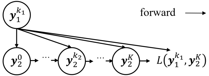
Figure 3: The computational graph corresponding to Eq. 34.

As the computational graph in Fig. 3 shows, we can expand $d\mathcal{L}(\bm{y}_{1}^{k_{1}},\bm{y}_{2}^{K})/d\bm{y}_{1}^{k_{1}}$ as:

$$\frac{d\mathcal{L}(\bm{y}_{1}^{k_{1}},\bm{y}_{2}^{K})}{d\bm{y}_{1}^{k_{1}}}=\underbrace{\frac{\partial\mathcal{L}(\bm{y}_{1}^{k_{1}},\bm{y}_{2}^{K})}{\partial\bm{y}_{1}^{k_{1}}}}_{\textrm{known}}+\sum_{k_{2}=0}^{K}\underbrace{\frac{\partial\bm{y}_{2}^{k_{2}}}{\partial\bm{y}_{1}^{k_{1}}}}_{\textrm{Eq.~{}}\ref{eq:yw_gd}}\underbrace{\frac{d\mathcal{L}(\bm{y}_{1}^{k_{1}},\bm{y}_{2}^{K})}{d\bm{y}_{2}^{k_{2}}}}_{\textrm{Eq.~{}}\ref{eq:yKyk_gd}}.$$ (34)

To solve Eq. 34, we first note that $\partial\mathcal{L}(\bm{y}_{1}^{k_{1}},\bm{y}_{2}^{K})/\partial\bm{y}_{1}^{k_{1}}$, $d\mathcal{L}(\bm{y}_{1}^{k_{1}},\bm{y}_{2}^{K})/d\bm{y}_{2}^{K}$ and $\partial\bm{y}_{2}^{0}/\partial\bm{y}_{1}^{k_{1}}$ is naturally known. Then, by taking partial derivative of the update rule of gradient ascent $\bm{y}_{2}^{k_{2}+1}\leftarrow\bm{y}_{2}^{k_{2}}+\alpha d\mathcal{L}(\bm{y}_{1}^{k_{1}},\bm{y}_{2}^{k_{2}})/d\bm{y}_{2}^{k_{2}}$ with regard to $\bm{y}_{1}^{k_{1}},\bm{y}_{2}^{k_{2}}$, we have:

$$\frac{\partial\bm{y}_{2}^{k_{2}+1}}{\partial\bm{y}_{2}^{k_{2}}}=I+\alpha\frac{\partial^{2}\mathcal{L}(\bm{y}_{1}^{k_{1}},\bm{y}_{2}^{k_{2}})}{\partial\bm{y}_{2}^{k_{2}}\partial\bm{y}_{2}^{k_{2}}},$$ (35)

$$\frac{\partial\bm{y}_{2}^{k_{2}+1}}{\partial\bm{y}_{1}^{k_{1}}}=\alpha\frac{\partial^{2}\mathcal{L}(\bm{y}_{1}^{k_{1}},\bm{y}_{2}^{k_{2}})}{\partial\bm{y}_{1}^{k_{1}}\partial\bm{y}_{2}^{k_{2}}}.$$ (36)

Note that Eq. 36 is the partial derivative $\partial\bm{y}_{2}^{k_{2}+1}/\partial\bm{y}_{1}^{k_{1}}$ instead of total derivative $d\bm{y}_{2}^{k_{2}+1}/d\bm{y}_{1}^{k_{1}}$, whose value is $(\partial\bm{y}_{2}^{k_{2}+1}/\partial\bm{y}_{2}^{k_{2}})(d\bm{y}_{2}^{k_{2}}/d\bm{y}_{1}^{k_{1}})+\partial\bm{y}_{2}^{k_{2}+1}/\partial\bm{y}_{1}^{k_{1}}$. And those second order terms can either be directly evaluated or approximated via finite difference as Eq. 38.

As Eq. 36 already solves the first term on the right hand side of Eq. 34, the remaining issue is $d\mathcal{L}(\bm{y}_{1}^{k_{1}},\bm{y}_{2}^{K})/d\bm{y}_{2}^{k_{2}}$. To solve this term, we expand it recursively as:

$$\frac{d\mathcal{L}(\bm{y}_{1}^{k_{1}},\bm{y}_{2}^{K})}{d\bm{y}_{2}^{k_{2}}}=\underbrace{\frac{\partial\bm{y}_{2}^{k_{2}+1}}{\partial\bm{y}_{2}^{k_{2}}}}_{\textrm{Eq.~{}}\ref{eq:yy_gd}}\frac{d\mathcal{L}(\bm{y}_{1}^{k_{1}},\bm{y}_{2}^{K})}{d\bm{y}_{2}^{k_{2}+1}}.$$ (37)

Then, we have solved all parts that is required to evaluate $\mathcal{L}(\bm{y}_{1}^{k_{1}},\bm{y}_{2}^{K})/d\bm{y}_{1}^{k_{1}}$. The above solving process can be described by the procedure grad-2-level($\bm{x},\bm{y}_{1}^{k_{1}}$) of Alg. 2. Specifically, the iterative update of $\overleftarrow{\bm{y}_{2}}^{k_{2}+1}$ corresponds to recursively expanding Eq. 37 with Eq. 35, and the iterative update of $\overleftarrow{\bm{y}_{1}}$ corresponds to recursively expanding Eq. 34 with Eq. 36 and Eq. 37. Upon the return of grad-2-level($\bm{x},\bm{y}_{1}^{k_{1}}$) of Alg. 2, we have $\overleftarrow{\bm{y}_{1}}=d\mathcal{L}(\bm{y}_{1}^{k_{1}},\bm{y}_{2}^{K})/d\bm{y}_{1}^{k_{1}}$.

The complexity of the Hessian-vector product in Alg. 2 may be reduced using finite difference following (Domke, 2012) as:

$$\frac{\partial^{2}\mathcal{L}(\bm{y}_{1}^{k_{1}},\bm{y}_{2}^{k_{2}})}{\partial\bm{y}_{1}^{k_{1}}\partial\bm{y}_{2}^{k_{2}}}\bm{v}=$$

$$\lim_{r\rightarrow 0}\frac{1}{r}( \frac{d\mathcal{L}(\bm{y}_{1}^{k_{1}},\bm{y}_{2}^{k_{2}}+r\bm{v})}{d\bm{y}_{1}^{k_{1}}}-\frac{d\mathcal{L}(\bm{y}_{1}^{k_{1}},\bm{y}_{2}^{k_{2}})}{d\bm{y}_{1}^{k_{1}}}),$$

$$\frac{\partial^{2}\mathcal{L}(\bm{y}_{1}^{k_{1}},\bm{y}_{2}^{k_{2}})}{\partial\bm{y}_{2}^{k_{2}}\partial\bm{y}_{2}^{k_{2}}}\bm{v}=$$

$$\lim_{r\rightarrow 0}\frac{1}{r}( \frac{d\mathcal{L}(\bm{y}_{1}^{k_{1}},\bm{y}_{2}^{k_{2}}+r\bm{v})}{d\bm{y}_{2}^{k_{2}}}-\frac{d\mathcal{L}(\bm{y}_{1}^{k_{1}},\bm{y}_{2}^{k_{2}})}{d\bm{y}_{2}^{k_{2}}}).$$ (38)

∎

Theorem 3.4. After the procedure grad-dag($\bm{x},\bm{y}_{0}^{k_{0}},...,\bm{y}_{i}^{k_{i}}$) in Alg. 3 executes, we have the return value $d\mathcal{L}(\bm{y}_{0}^{k_{0}},...,\bm{y}_{i}^{k_{i}},\bm{y}_{>i}^{K})/d\bm{y}_{i}^{k_{i}}=\overleftarrow{\bm{y}_{i}}$.

Proof.

Consider computing the target gradient with DAG $\mathcal{G}$. The $\bm{y}_{i}$’s gradient is composed of its own contribution to $\mathcal{L}$ in addition to the gradient from its children $\bm{y}_{j}\in\mathcal{C}(\bm{y}_{i})$. Further, as we are considering the optimized children $\bm{y}_{j}^{K}$, we expand each child node $\bm{y}_{j}$ as Fig. 3. Then, we have:

$$\frac{d\mathcal{L}(\bm{y}_{0}^{k_{0}},...,\bm{y}_{i}^{k_{i}},\bm{y}_{>i}^{K})}{d\bm{y}_{i}^{k_{i}}} =\underbrace{\frac{\partial\mathcal{L}(\bm{y}_{0}^{k_{0}},...,\bm{y}_{i}^{k_{i}},\bm{y}_{>i}^{K})}{\partial\bm{y}_{i}^{k_{i}}}}_{\textrm{known}}$$

$$+\sum_{\bm{y}_{j}\in\mathcal{C}(\bm{y}_{i})}(\sum_{k_{j}=0}^{K} \underbrace{\frac{\partial\bm{y}_{j}^{k_{j}}}{\partial\bm{y}_{i}^{k_{i}}}}_{\textrm{Eq.~{}}\ref{eq:yw_gd}}\underbrace{\frac{d\mathcal{L}(\bm{y}_{0}^{k_{0}},...,\bm{y}_{j-1}^{k_{j-1}},\bm{y}_{\geq j}^{K})}{d\bm{y}_{j}^{k_{j}}}}_{\textrm{Eq.~{}}\ref{eq:yKyk_gd}}).$$ (39)

The first term on the right-hand side of Eq. 39 can be trivially evaluated. The $\partial\bm{a}_{j}^{k_{j}}/\partial\bm{a}_{i}^{k_{i}}$ can be evaluated as Eq. 36 from the proof of Theorem. 3.3. The $d\mathcal{L}(\bm{a}_{0}^{k_{0}},...,\bm{a}_{j-1}^{k_{j-1}},\bm{a}_{\geq j}^{K})/d\bm{a}_{j}^{k_{j}}$ can also be iteratively expanded as Eq. 37 from the proof of Theorem. 3.3. Then, the rest of proof follows Theorem. 3.3 to expand Eq. 36 and Eq. 37.

We highlight several key differences between Alg. 3 and Alg. 2:

• The gradient evaluation of current node $\bm{y}_{i}$ requires gradient of its plural direct children $\bm{y}_{j}\in\mathcal{C}(\bm{y}_{i})$, instead of the single child in 2-level case. The children traversal part of Eq. 37 corresponds to the two extra for in Alg. 3.

• The gradient ascent update of child latent parameter $\bm{y}_{j}^{k_{j}+1}\leftarrow\bm{y}_{j}^{k_{j}}+\alpha d\mathcal{L}(\bm{y}_{0}^{k_{0}},...,\bm{y}_{j}^{k_{j}},\bm{y}_{>j}^{K})/d\bm{y}_{j}^{k_{j}}$ can be conducted trivially only if $\mathcal{C}(\bm{y}_{j})$ is empty, otherwise the gradient has to be evaluated recursively using Eq. 39. And this part corresponds to the recursive call in line 11 of Alg. 3.

And the other part of Alg. 3 is the same as Alg. 2. So the rest of the proof follows Theorem. 3.3. Similarly, the Hessian-vector product can be approximated as Eq. 38. However, this does not save Alg. 3 from an overall complexity of $\Theta(K^{N})$.

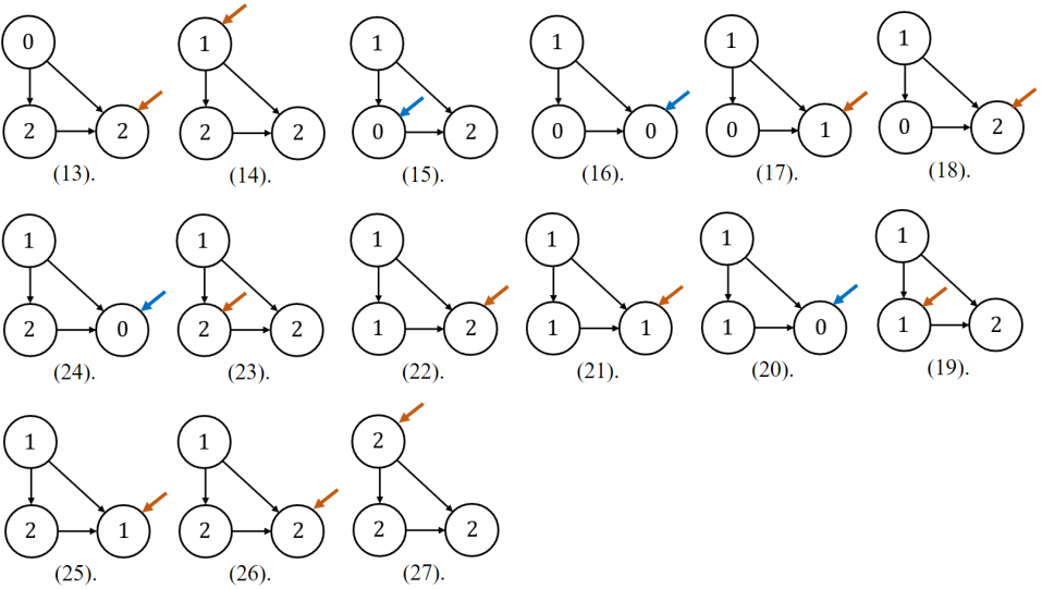
Figure 7: (0). The example setup. (1).-(27). The execution procedure. The number in the circle indicates the gradient step $k_{i}$ of each node $\bm{y}_{i}$. The bold blue/red arrow indicates that the current node is under initialization/gradient ascent.

To better understand Alg. 3, we provide an example of the full procedure of its execution in Fig. 7. The setup is as Fig. 7.(0): we have $N=3$ latent $\bm{y}_{1},\bm{y}_{2},\bm{y}_{3}$ and gradient ascent step $K=2$, connected by a DAG shown in the figure. ∎

Appendix C Implementation Details

C.1 Implementation Details of Density Estimation

For density estimation experiment, we follow the training details of Burda et al. (2015). We adopt Adam (Kingma & Ba, 2014) optimizer with $\beta_{1}=0.9,\beta_{2}=0.999,\epsilon=1e-4$ and batch-size $20$. We adopt the same learning rate scheduler as (Burda et al., 2015) and train 3280 epochs for total. All likelihood results in Tab. 2 are evidence lowerbound. And the binarization of MNIST dataset follows (Salakhutdinov & Murray, 2008).

C.2 Implementation Details of Bit Allocation

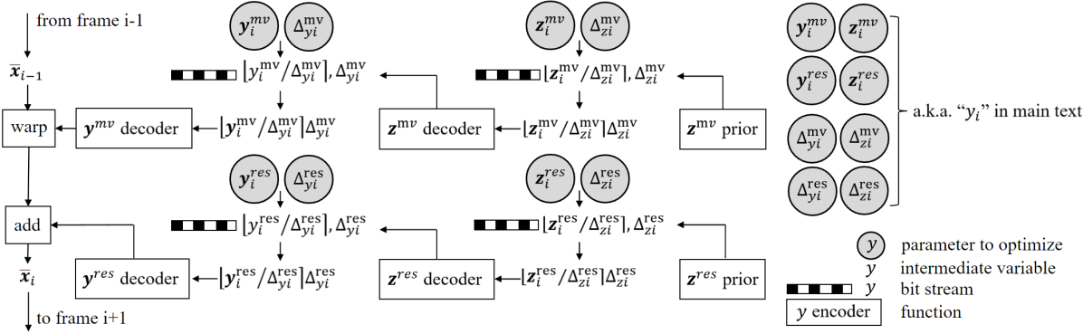
Figure 4: Overall framework of detailed implementation based on DVC (Lu et al., 2019). The DCVC’s (Li et al., 2021) framework is very similar.

In the main text and analysis, we use $\bm{y}_{i}$ to abstractly represent all the latent of frame $i$. While the practical implementation is more complicated. In fact, the actual latent is divided into 8 parts: the first level of residual latent $\bm{y}_{i}^{res}$, the second level of residual latent $\bm{z}_{i}^{res}$, the first level of optical flow latent $\bm{y}_{i}^{mv}$, and the second level of optical flow latent $\bm{z}_{i}^{mv}$. In addition to those 4 latent, we also include quantization stepsize $\Delta_{iy}^{res},\Delta_{iz}^{res},\Delta_{iy}^{mv},\Delta_{iz}^{mv}$ as Choi et al. (2019) for DVC (Lu et al., 2019) and DCVC (Li et al., 2021). For HSTEM (Li et al., 2022a), those quantization parameters are predicted from the latent $\bm{z}_{i}$, so we have not separately optimize them. This is shown in the overall framework diagram as Fig. 4. To re-parameterize the quantization, we adopt Stochastic Gumbel Annealing with the hyper-parameters as Yang et al. (2020b).

Appendix D More Experimental Results

D.1 R-D Performance

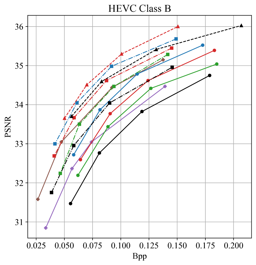
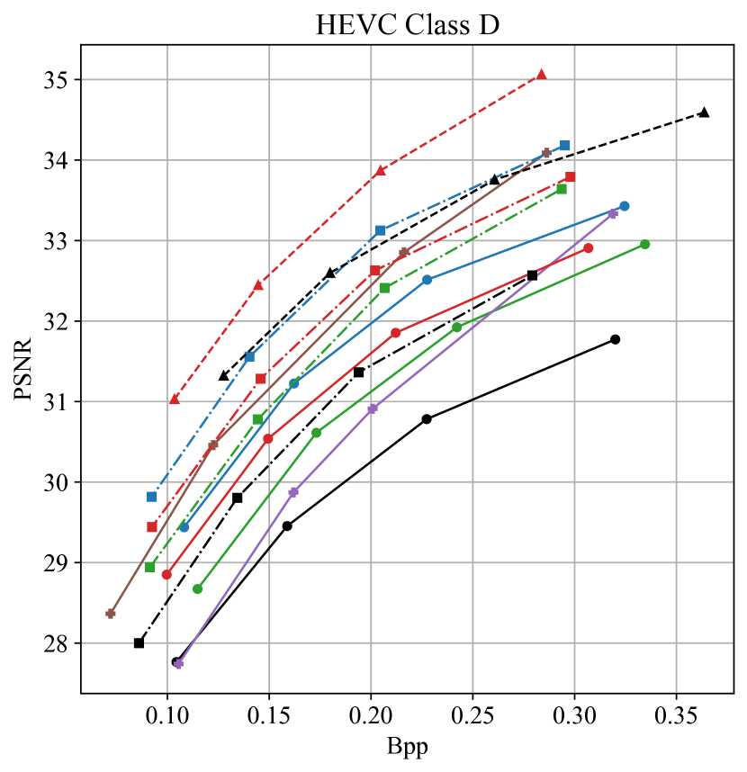
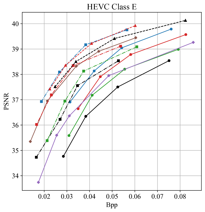
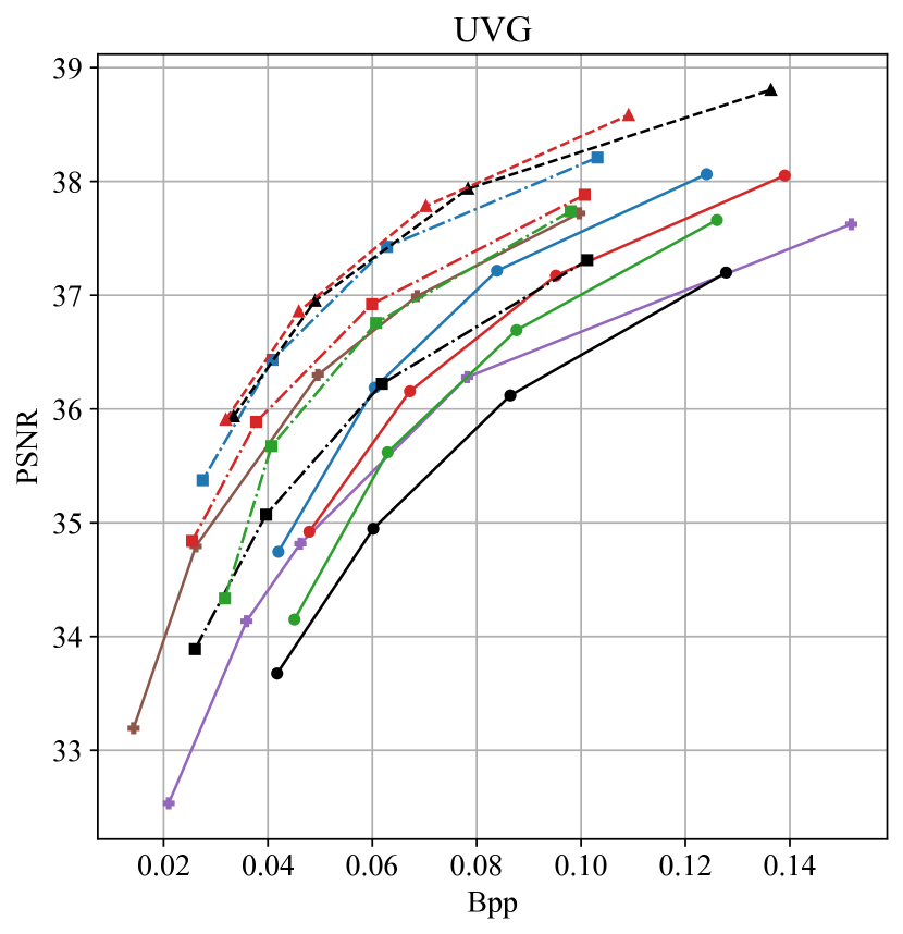
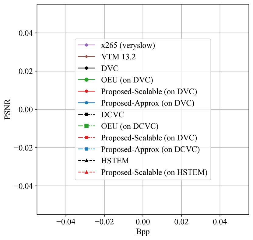
Figure 6: The R-D performance of our approach compared with baselines (w/o bit allocation) and other bit allocation approach.

Fig. 6 shows the R-D curves of proposed approach, other bit allocation approach (Lu et al., 2020a) and baselines (Lu et al., 2019; Li et al., 2021, 2022a), from which we observe that proposed approach has stable improvement upon three baselines and five datasets (HEVC B/C/D/E, UVG).

In addition to baselines and bit allocation results, we also show the R-D performance of traditional codecs. For H.265, we test x256 encoder with veryslow preset. For H.266, we test VTM 13.2 with lowdelay P preset. The command lines for x265 and VTM are as follows:

ffmpeg -y -pix_fmt yuv420p -s HxW
-r 50 -i src_yuv -vframes frame_cnt
-c:v libx265 -preset veryslow
-x265-params "qp=qp:
keyint=gop_size" output_bin

EncoderApp -c encoder_lowdelay_P_vtm.cfg
--QP=qp --InputFile=src_yuv
--BitstreamFile=output_bin
--DecodingRefreshType=2
--InputBitDepth=8
--OutputBitDepth=8
--OutputBitDepthC=8
--InputChromaFormat=420
--Level=6.2 --FrameRate=50
--FramesToBeEncoded=frame_cnt
--SourceWidth=W
--SourceHeight=H

And for x265, we test qp=$\{38,34,32,28,24\}$. For VTM 13.2, we test qp=$\{34,30,26,24,22\}$.

As Fig. 6 shows, with our bit allocation, the DCVC (Li et al., 2021) outperforms the latest traditional codec standard (VTM 13.2). The HSTEM baseline (Li et al., 2022a) already outperforms VTM 13.2, and our bit allocation makes this advantage more obvious.

D.2 Qualitative Results

In Fig. 8, Fig. 9, Fig. 10 and Fig. 11, we present the qualitative result of our approach compared with the baseline approach on HEVC Class D. We note that compared with the reconstruction frame of baseline approach, the reconstruction frame of our proposed approach preserves significantly more details with lower bitrate, and looks much more similar to the original frame.

Appendix E More on Online Encoder Update (OEU)

E.1 Why OEU is a Frame-level Bit Allocation

The online encoder update (OEU) of Lu et al. (2020a) is proposed to resolve the error propagation. It fits into the line of works on encoder over-fitting (Cremer et al., 2018; van Rozendaal et al., 2021; Zou et al., 2020) and does not fit into the SAVI framework. However, it can be seen as an intermediate point between fully-amortized variational inference (FAVI) and SAVI: FAVI uses the same inference model parameter $\phi$ for all frames; SAVI performs stochastic variational inference on variational posterior parameter $\bm{y}_{i}$ per frame, which is the finest-granularity finetune possible for latent variable model; And Lu et al. (2020a) finetune inference model parameter $\phi_{i}$ per-frame. It is less computational expensive but also performs worse compared with our method based on SAVI (See Tab. 5). However, it is more computational expensive and performs better compared with FAVI (or NVC without bit allocation).

	DVC	OEU	Proposed-Scalable (Sec. 4.2)	Proposed-Approx (Sec. 4.1)
Parameter	-	$\phi_{i}$	$\bm{y}_{i}$	$\bm{y}_{i}$
Granularity	-	frame-level	pixel-level	pixel-level
# of parameter	0	$\Theta(N|\phi|)$	$\Theta(NHW)$	$\Theta(NHW)$
$K$ required	0	$\approx 50$	$\approx 2000$	$\approx 2000$
R-D performance	poor	middle	good	very good
Temporal complexity	$\Theta(N)$	$\Theta(KN)$	$\Theta(KN)$	$\Theta(KN)$
Spatial complexity	$\Theta(1)$	$\Theta(N)$	$\Theta(1)$	$\Theta(N)$
Encoding time	fast	middle	slow	very slow
Decoding time	same	same	same	same

Table 5: A comparison between DVC (FAVI, w/o bit allocation), OEU (Lu et al., 2020a) and our proposed bit allocation (SAVI) approach. $N$ is the GoP size, $|\phi|$ is the number of encoder parameters, $H\times W$ is the number of pixels, $K$ is number of iteration.

Although OEU does not fit into SAVI framework, still it can be written as Eq. 40, which is very similar to our SAVI-based implicit bit allocation with $\Delta_{i}$ removed and optimization target changed from $\bm{y}_{i},\Delta_{i}$ to encoder parameter $\phi_{i}$.

$$\phi_{1:K}^{*}\leftarrow\arg\max_{\phi_{1:K}}\mathcal{L}$$ (40)

This similarity also implies that Lu et al. (2020a) is optimized towards the overall bit allocation target. Thus, it is also an optimal bit allocation. However, the encoder parameter $\phi_{i}$ is only sensitive to the location of a frame inside a GoP. It can not sense the pixel location and pixel-level reference structure. So the bit allocation of Lu et al. (2020a) is limited to frame-level instead of pixel-level like ours.

Despite it is not pixel-level optimal bit allocation, OEU (Lu et al., 2020a) is indeed the true pioneer of bit allocation in NVC. However, the authors of Lu et al. (2020a) have not mentioned the concept of bit allocation in the original paper, which makes it a secret pioneer of bit allocation for NVC until now.

E.2 Why OEU is not an Error Propagation Aware Strategy

One problem of NVC is that the frame quality drops rapidly with the frame index $t$ inside the GoP. Many works call this phenomena error propagation (Lu et al., 2020a; Sun et al., 2021; Sheng et al., 2021), including the OEU. And the error propagation aware technique is subtly related to bit allocation.

Figure 5: The comparison between ideal error propagation aware and ideal bit allocation.

In this paper, we would like to distinguish error propagation aware technique and bit allocation formally: error propagation aware technique aims to solve the problem of quality drop with frame index $t$, and an ideal solution to error propagation should produce a horizontal quality-t curve, just like the red line in Fig. 5. And Sun et al. (2021) aim to solve error propagation instead of bit allocation, as their frame quality is consistent to frame index $t$. However, the aim of bit allocation is to produce the best average R-D cost. And due to the frame reference structure, the frame quality of ideal bit allocation should drop with frame index $t$. As a result, the quality degrading rate of ideal bit allocation is less steep than vanilla NVC, but it almost never falls horizontal.

From the old school bitrate control’s perspective (Tagliasacchi et al., 2008), the target of avoiding error propagation is minVar, which means that we want to minimize the quality fluctuation between frames. On the other hand, the target of bit allocation is minAvg, which means that we want to minimize the average distortion under constrain of bitrate. And usually, those two targets are in odd with each other.

However, the results of a crippled error propagation aware method and an optimal bit allocation are similar: the degradation speed of quality-$t$ curve is decreased but not flattened. And thus, sometimes the result of an optimal bit allocation is likely to be recognised as an unsuccessful error propagation aware method. This similarity has disorientated Lu et al. (2020a) to falsely classify themselves into error propagation aware strategy instead of bit allocation.

As we empirically show in Fig. 2.lower-left, the quality-$t$ curves of both our proposed method and OEU are not horizontal. Instead, they are just less steep than the original DVC (Lu et al., 2019). This phenomena further verifies that OEU is essentially a bit allocation, instead of an error propagation aware strategy.

Appendix F More Discussion

F.1 More Limitations

As we have stated in main text, the major limitation of our method is encoding complexity. Although the decoding time is not influenced, our method requires iterative gradient descent during encoding. Practically, our approach is limited to scenarios when R-D performance matters more than encoding time (e.g. content delivery network). Or it can also be used as a benchmark for research on faster bit allocation methods.

F.2 Ethics Statement

Improving the R-D performance of NVC has valuable social impact. First, better R-D performance means less resources required for video storage and transmission. Considering the amount of video produced everyday, it is beneficial to the environment if we could save those resources by improving codec. Second, the traditional codec requires dedicated hardware decoder for efficient decoding, while NVC could utilize the universal neural accelerator. The improvement of neural codec can be readily deployed without hardware up-gradation.

Figure 8: Qualitative results using BasketballPass of HEVC Class D. Top. Original frame. Middle. Baseline codec (DVC)’s reconstruction result with bpp $=0.148$ and PSNR $=33.06$dB. Bottom. Proposed method’s reconstruction result with bpp $=0.103$ and PSNR $=34.91$dB.

Figure 9: Qualitative results using BlowingBubbles of HEVC Class D. Top. Original frame. Middle. Baseline codec (DVC)’s reconstruction result with bpp $=0.206$ and PSNR $=30.71$dB. Bottom. Proposed method’s reconstruction result with bpp $=0.129$ and PSNR $=32.34$dB.

Figure 10: Qualitative results using BQSquare of HEVC Class D. Top. Original frame. Middle. Baseline codec (DVC)’s reconstruction result with bpp $=0.232$ and PSNR $=28.72$dB. Bottom. Proposed method’s reconstruction result with bpp $=0.128$ and PSNR $=30.87$dB.

Figure 11: Qualitative results using RaceHorses of HEVC Class D. Top. Original frame. Middle. Baseline codec (DVC)’s reconstruction result with bpp $=0.448$ and PSNR $=30.48$dB. Bottom. Proposed method’s reconstruction result with bpp $=0.379$ and PSNR $=31.92$dB.

References

- Agustsson et al. (2020) Agustsson, E., Minnen, D., Johnston, N., Balle, J., Hwang, S. J., and Toderici, G. Scale-space flow for end-to-end optimized video compression. In Proc. IEEE Comput. Soc. Conf. Comput. Vis. Pattern Recognit, pp. 8503–8512, 2020.
- Ballé et al. (2016) Ballé, J., Laparra, V., and Simoncelli, E. P. End-to-end optimized image compression. arXiv preprint arXiv:1611.01704, 2016.
- Bégaint et al. (2020) Bégaint, J., Racapé, F., Feltman, S., and Pushparaja, A. Compressai: a pytorch library and evaluation platform for end-to-end compression research. arXiv preprint arXiv:2011.03029, 2020.
- Bjontegaard (2001) Bjontegaard, G. Calculation of average psnr differences between rd-curves. VCEG-M33, 2001.
- Blei et al. (2017) Blei, D. M., Kucukelbir, A., and McAuliffe, J. D. Variational inference: A review for statisticians. Journal of the American statistical Association, 112(518):859–877, 2017.
- Bossen et al. (2013) Bossen, F. et al. Common test conditions and software reference configurations. JCTVC-L1100, 12(7), 2013.
- Bross et al. (2021) Bross, B., Chen, J., Ohm, J.-R., Sullivan, G. J., and Wang, Y.-K. Developments in international video coding standardization after avc, with an overview of versatile video coding (vvc). Proc. IEEE, 109(9):1463–1493, 2021.
- Burda et al. (2015) Burda, Y., Grosse, R., and Salakhutdinov, R. Importance weighted autoencoders. arXiv preprint arXiv:1509.00519, 2015.
- Cetin et al. (2022) Cetin, E., Yılmaz, M. A., and Tekalp, A. M. Flexible-rate learned hierarchical bi-directional video compression with motion refinement and frame-level bit allocation. arXiv e-prints, pp. arXiv–2206, 2022.
- Cheng et al. (2020) Cheng, Z., Sun, H., Takeuchi, M., and Katto, J. Learned image compression with discretized gaussian mixture likelihoods and attention modules. In Proc. IEEE Comput. Soc. Conf. Comput. Vis. Pattern Recognit, pp. 7939–7948, 2020.
- Choi et al. (2019) Choi, Y., El-Khamy, M., and Lee, J. Variable rate deep image compression with a conditional autoencoder. In Proc. IEEE Int. Conf. Comput. Vis., pp. 3146–3154. IEEE, 2019.
- Cremer et al. (2018) Cremer, C., Li, X., and Duvenaud, D. Inference suboptimality in variational autoencoders. In Int. Conf. on Machine Learning, pp. 1078–1086. PMLR, 2018.
- Djelouah et al. (2019) Djelouah, A., Campos, J., Schaub-Meyer, S., and Schroers, C. Neural inter-frame compression for video coding. In Proc. IEEE Int. Conf. Comput. Vis., October 2019.
- Djelouah & Schroers (2019) Djelouah, J. C. M. S. A. and Schroers, C. Content adaptive optimization for neural image compression. In Proc. IEEE Comput. Soc. Conf. Comput. Vis. Pattern Recognit, 2019.
- Domke (2012) Domke, J. Generic methods for optimization-based modeling. In Artificial Intelligence and Statistics, pp. 318–326. PMLR, 2012.
- Gao et al. (2022) Gao, C., Xu, T., He, D., Wang, Y., and Qin, H. Flexible neural image compression via code editing. In Advances in Neural Information Processing Systems, 2022.
- Hu et al. (2022) Hu, Z., Lu, G., Guo, J., Liu, S., Jiang, W., and Xu, D. Coarse-to-fine deep video coding with hyperprior-guided mode prediction. In Proc. IEEE Comput. Soc. Conf. Comput. Vis. Pattern Recognit, pp. 5921–5930, 2022.
- Kim et al. (2018) Kim, Y., Wiseman, S., Miller, A., Sontag, D., and Rush, A. Semi-amortized variational autoencoders. In Int. Conf. on Machine Learning, pp. 2678–2687. PMLR, 2018.
- Kingma & Ba (2014) Kingma, D. P. and Ba, J. Adam: A method for stochastic optimization. CoRR, abs/1412.6980, 2014.
- Kingma & Welling (2013) Kingma, D. P. and Welling, M. Auto-encoding variational bayes. arXiv preprint arXiv:1312.6114, 2013.
- Koller & Friedman (2009) Koller, D. and Friedman, N. Probabilistic graphical models: principles and techniques. MIT press, 2009.
- LeCun et al. (1998) LeCun, Y., Bottou, L., Bengio, Y., and Haffner, P. Gradient-based learning applied to document recognition. Proceedings of the IEEE, 86(11):2278–2324, 1998.
- Li et al. (2014) Li, B., Li, H., Li, L., and Zhang, J. domain rate control algorithm for high efficiency video coding. IEEE Trans. Image Process., 23(9):3841–3854, 2014.
- Li et al. (2021) Li, J., Li, B., and Lu, Y. Deep contextual video compression. Advances in Neural Information Processing Systems, 34, 2021.
- Li et al. (2022a) Li, J., Li, B., and Lu, Y. Hybrid spatial-temporal entropy modelling for neural video compression. In Proceedings of the 30th ACM International Conference on Multimedia, MM ’22, pp. 1503–1511, New York, NY, USA, 2022a. Association for Computing Machinery. ISBN 9781450392037. doi: 10.1145/3503161.3547845. URL https://doi.org/10.1145/3503161.3547845.
- Li et al. (2023) Li, J., Li, B., and Lu, Y. Neural video compression with diverse contexts. arXiv preprint arXiv:2302.14402, 2023.
- Li et al. (2016) Li, L., Li, B., Li, H., and Chen, C. W. -domain optimal bit allocation algorithm for high efficiency video coding. IEEE Trans. Circuits Syst. Video Technol., 28(1):130–142, 2016.
- Li et al. (2020) Li, Y., Liu, Z., Chen, Z., and Liu, S. Rate control for versatile video coding. In IEEE Int. Conf. on Image Process., pp. 1176–1180. IEEE, 2020.
- Li et al. (2022b) Li, Y., Chen, X., Li, J., Wen, J., Han, Y., Liu, S., and Xu, X. Rate control for learned video compression. In ICASSP 2022-2022 IEEE Int. Conf. on Acoustics, Speech and Signal Processing (ICASSP), pp. 2829–2833. IEEE, 2022b.
- Lin et al. (2020) Lin, J., Liu, D., Li, H., and Wu, F. M-lvc: Multiple frames prediction for learned video compression. In Proc. IEEE Comput. Soc. Conf. Comput. Vis. Pattern Recognit, pp. 3546–3554, 2020.
- Lu et al. (2019) Lu, G., Ouyang, W., Xu, D., Zhang, X., Cai, C., and Gao, Z. Dvc: An end-to-end deep video compression framework. In Proc. IEEE Comput. Soc. Conf. Comput. Vis. Pattern Recognit, pp. 11006–11015, 2019.
- Lu et al. (2020a) Lu, G., Cai, C., Zhang, X., Chen, L., Ouyang, W., Xu, D., and Gao, Z. Content adaptive and error propagation aware deep video compression. In European Conference on Computer Vision, pp. 456–472. Springer, 2020a.
- Lu et al. (2020b) Lu, G., Zhang, X., Ouyang, W., Chen, L., Gao, Z., and Xu, D. An end-to-end learning framework for video compression. IEEE Trans. Pattern Anal. Mach. Intell, 43(10):3292–3308, 2020b.
- Marino et al. (2018) Marino, J., Yue, Y., and Mandt, S. Iterative amortized inference. In Int. Conf. on Machine Learning, pp. 3403–3412. PMLR, 2018.
- Mercat et al. (2020) Mercat, A., Viitanen, M., and Vanne, J. Uvg dataset: 50/120fps 4k sequences for video codec analysis and development. In Proceedings of the 11th ACM Multimedia Systems Conference, pp. 297–302, 2020.
- Minnen et al. (2018) Minnen, D., Ballé, J., and Toderici, G. D. Joint autoregressive and hierarchical priors for learned image compression. Advances in neural information processing systems, 31, 2018.
- Rippel et al. (2019) Rippel, O., Nair, S., Lew, C., Branson, S., Anderson, A. G., and Bourdev, L. Learned video compression. In Proceedings of the IEEE/CVF International Conference on Computer Vision, pp. 3454–3463, 2019.
- Salakhutdinov & Murray (2008) Salakhutdinov, R. and Murray, I. On the quantitative analysis of deep belief networks. In International Conference on Machine Learning, 2008.
- Samuel & Tappen (2009) Samuel, K. G. and Tappen, M. F. Learning optimized map estimates in continuously-valued mrf models. In 2009 IEEE Conference on Computer Vision and Pattern Recognition, pp. 477–484. IEEE, 2009.
- Sheng et al. (2021) Sheng, X., Li, J., Li, B., Li, L., Liu, D., and Lu, Y. Temporal context mining for learned video compression. arXiv preprint arXiv:2111.13850, 2021.
- Sun et al. (2021) Sun, Z., Tan, Z., Sun, X., Zhang, F., Li, D., Qian, Y., and Li, H. Spatiotemporal entropy model is all you need for learned video compression. arXiv preprint arXiv:2104.06083, 2021.
- Tagliasacchi et al. (2008) Tagliasacchi, M., Valenzise, G., and Tubaro, S. Minimum variance optimal rate allocation for multiplexed h. 264/avc bitstreams. IEEE Trans. Image Process., 17(7):1129–1143, 2008.
- Tishby et al. (2000) Tishby, N., Pereira, F. C., and Bialek, W. The information bottleneck method. arXiv preprint physics/0004057, 2000.
- van Rozendaal et al. (2021) van Rozendaal, T., Huijben, I. A., and Cohen, T. S. Overfitting for fun and profit: Instance-adaptive data compression. arXiv preprint arXiv:2101.08687, 2021.
- Yang et al. (2020a) Yang, R., Yang, Y., Marino, J., and Mandt, S. Hierarchical autoregressive modeling for neural video compression. arXiv preprint arXiv:2010.10258, 2020a.
- Yang et al. (2020b) Yang, Y., Bamler, R., and Mandt, S. Improving inference for neural image compression. Advances in Neural Information Processing Systems, 33:573–584, 2020b.
- Yılmaz & Tekalp (2021) Yılmaz, M. A. and Tekalp, A. M. End-to-end rate-distortion optimized learned hierarchical bi-directional video compression. IEEE Trans. Image Process., 31:974–983, 2021.
- Zhao et al. (2021) Zhao, J., Li, B., Li, J., Xiong, R., and Lu, Y. A universal encoder rate distortion optimization framework for learned compression. In Proc. IEEE Comput. Soc. Conf. Comput. Vis. Pattern Recognit, pp. 1880–1884, 2021.
- Zou et al. (2020) Zou, N., Zhang, H., Cricri, F., Tavakoli, H. R., Lainema, J., Hannuksela, M., Aksu, E., and Rahtu, E. L 2 c–learning to learn to compress. In 2020 IEEE 22nd International Workshop on Multimedia Signal Processing (MMSP), pp. 1–6. IEEE, 2020.