Numerical Solution of the 3-D Travel Time Tomography Problem

Abstract

The first numerical solution of the 3-D travel time tomography problem is presented. The globally convergent convexification numerical method is applied.

1 Introduction

In this paper the first 3-D computational result is obtained for the Travel Time Tomography Problem (TTTP). We apply a globally convergent, the so-called convexification method. Two versions of the theory of this method for the TTTP were developed in [22, 23]. We use the version of [22], which is also fully described in the book [26, Chapter 11].

All functions considered below are real valued ones. Below $\mathbf{x}=\left(x,y,z\right)$ denotes points in $\mathbb{R}^{3}.$ Let $\Omega\subset\mathbb{R}^{3}$ be a bounded domain and let $S\subset\mathbb{R}^{3},$ $S\cap\overline{\Omega}=\varnothing$ be a surface, on a part $L_{\text{src}}\subseteq S$ of which wave sources are located. Let $c\left(\mathbf{x}\right)$ be the speed of waves propagation, $c\left(\mathbf{x}\right)=1/n\left(\mathbf{x}\right)$, where $n\left(\mathbf{x}\right)$ is the refractive index. Let $m\left(\mathbf{x}\right)=n^{2}\left(\mathbf{x}\right).$ The function $m\left(\mathbf{x}\right)$ generates the Riemannian metric [31, Chapter 3]

$$d\tau=\sqrt{m\left(\mathbf{x}\right)}\sqrt{\left(dx\right)^{2}+\left(dy\right)^{2}+\left(dz\right)^{2}}.$$

The time, which the wave needs to propagate from a source $\mathbf{x}_{0}\in L_{\text{src}}$ to a point $\mathbf{x}$ is called the the “first arrival time” or “travel time”. In the case of a heterogeneous medium with $m\left(\mathbf{x}\right)\neq const.,$ the first arriving signal, which arrives at the arrival time to the point $\mathbf{x}$, propagates not along the straight line connecting points $\mathbf{x}$ and $\mathbf{x}_{0}$ but rather along the geodesic line $\Gamma\left(\mathbf{x},\mathbf{x}_{0}\right)$ generated by this metric and connecting points $\mathbf{x}$ and $\mathbf{x}_{0}$. The travel time $\tau\left(\mathbf{x},\mathbf{x}_{0}\right)$ is

$$\tau\left(\mathbf{x},\mathbf{x}_{0}\right)=\mathop{\displaystyle\int}\limits_{\Gamma\left(\mathbf{x},\mathbf{x}_{0}\right)}\sqrt{m\left(\mathbf{y}\left(s\right)\right)}ds,$$ (1.1)

where $ds$ is the element of the euclidean length. The function $\tau\left(\mathbf{x},\mathbf{x}_{0}\right)$ satisfies the so-called eikonal equation [31, Chapter 3]

$$\left(\nabla_{\mathbf{x}}\tau\right)^{2}=m\left(\mathbf{x}\right),$$ (1.2)

$$\tau\left(\mathbf{x},\mathbf{x}_{0}\right)=O\left(\left|\mathbf{x}-\mathbf{x}_{0}\right|\right)\text{ as }\mathbf{x}\rightarrow\mathbf{x}_{0}.$$ (1.3)

The Travel Time Tomography Problem (TTTP) is one of Coefficient Inverse Problems (CIPs) for PDEs. Another name for TTTP is Inverse Kinematic Problem [31, Chapter 3].

Travel Time Tomography Problem (TTTP). Suppose that the function $m\left(\mathbf{x}\right)$ is given outside of the domain $\Omega.$ Given boundary measurements $g\left(\mathbf{x},\mathbf{x}_{0}\right)$ of the function $\tau\left(\mathbf{x},\mathbf{x}_{0}\right),$

$$\tau\left(\mathbf{x},\mathbf{x}_{0}\right)=g\left(\mathbf{x},\mathbf{x}_{0}\right),\text{ }\mathbf{x}\in\partial\Omega,\mathbf{x}_{0}\in L_{\text{src}},$$ (1.4)

find the function $m\left(\mathbf{x}\right)$ for $\mathbf{x}\in\Omega.$

Thus, the governing eikonal PDE (1.2) with condition (1.3) is nonlinear, its right hand side is unknown and geodesic lines $\Gamma\left(\mathbf{x},\mathbf{x}_{0}\right)$ in (1.1) are unknown as well. These three factors cause quite substantial challenges in attempts to solve this problem.

TTTP has well known applications in the problem of the recovery of the speed of propagation of seismic waves inside the Earth [10, 31, 36, 37]. Some other applications are in the phaseless inverse scattering problem [19], in the problem of detection and identification of underwater objects, and in the problem of standoff inspection of buildings if using transmitted time resolved electromagnetic data [27]. The first solution of TTTP was obtained by Herglotz in 1905 [10] and then by Wiechert and Zoeppritz [37] in 1907. In these pioneering works the above application to geophysics was considered, and the underlying mathematical model was 1-D.  A detailed description of the method of [10, 37] can be found in [31, section 3 of Chapter 3].

The $n-$D case, $n=2,3,$ is mathematically far more challenging than the 1-D case. We refer to [33], where a numerical method was developed and tested in the 2-D case. In [38] another numerical method was developed analytically in the $n-$D, $n=2,3$ case and tested numerically in the 2$-$D case. In [24] a numerical method with a guaranteed convergence was developed for the linearized TTTP in the $n-$D case, assuming that the function $m\left(\mathbf{x}\right)=m_{0}\left(\mathbf{x}\right)+m_{1}\left(\mathbf{x}\right),$ where $m_{0}\left(\mathbf{x}\right)$ is known, $m_{1}\left(\mathbf{x}\right)$ is unknown and $\left|m_{1}\left(\mathbf{x}\right)\right|<<m_{0}\left(\mathbf{x}\right),$ in which case geodesic lines were known and generated by the function $m_{0}\left(\mathbf{x}\right),$ and the problem became linearized, see [31, Chapter 3] for a discussion of the importance of the linearized case. In [24], numerical studies were carried out in the 2$-$D case.

The authors are unaware about numerical results for TTTP in the full nonlinear 3-D case, which would be supplied by the rigorous global convergence analysis. The goal of the current paper is to obtain such numerical results. As mentioned above, we implement numerically here the globally convergent convexification method for the 3-D TTTP. The theory of this method was published in [22] and [26, Chapter 11]. Our data are formally determined ones. This means that the number $k$ of free variables in the data equals the number $n$ of free variables in the unknown function $m\left(\mathbf{x}\right),k=n=3.$ Also, our data are incomplete. Indeed, in the case of complete data, the source should run somewhat around the domain $\Omega.$ Unlike this, in our case $L_{\text{src}}\in\mathbb{R}^{3}\diagdown\Omega$ is an interval of a straight line.

All CIPs are both nonlinear and ill-posed. Conventional numerical methods for CIPs are based on minimizations of least squares cost functionals, see, e.g. [6, 7, 8]. However, nonlinearity and ill-posedness of CIPs cause non convexity of these functionals, which, in turn typically leads to the phenomenon of multiple local minima and ravines, see, e.g. [32] for a numerical example of this phenomenon. However, since any gradient-like method of the optimization of that functional can stop at any point of a local minimum, which might be located far from the solution, then it is worth to address that phenomenon. This is done by the convexification concept.

The convexification concept was originally proposed in [16, 17] to avoid the above phenomenon. Results of [16, 17] are only analytical ones. Active numerical studies of various of versions of this concept have started from the work [1], which has removed some obstacles for numerical implementations. We refer here to, e.g. [13, 21, 25, 26, 28, 29] as some samples of these publications, also, see references cited therein as well as the recent book [26]. The convexification significantly modifies the idea of the paper [5], in which the tool of Carleman estimates was introduced in the field of inverse problems for the first time, see, e.g. books [2, 3, 11, 26, 30] for Carleman estimates. The idea of [5] has generated a number of publications of many authors, which have discussed questions of uniqueness and stability results for CIPs, see, e.g. [2, 3, 11, 14, 15, 18, 26, 39] and references cited therein. Thus, convexification stands aside of those publications, since it is dedicated to the numerical extension of the idea of [5]. The numerical issue was not discussed in [5].

Given a CIP for a PDE, the convexification constructs a weighted Tikhonov-like least squares cost functional $J_{\lambda}$ with the Carleman Weight Function (CWF) in it. This is the function which is used as the weight in the Carleman estimate for that PDE operator. Here $\lambda\geq 1$ is the parameter of the CWF. This functional is considered on a certain convex bounded set $S\left(d\right)\subset H,$ where $d$ is the diameter of this set and $H$ is an appropriate Hilbert space. The central theorem for each version of the convexification is the one, which claims that if $\lambda$ is sufficiently large, then $J_{\lambda}$ is strictly convex on $S\left(d\right)$ and has unique minimizer on $\overline{S\left(d\right)}.$ Next, a theorem is proven, which claims convergence to that unique minimizer of either the gradient projection or the gradient descent method of the minimization of $J_{\lambda}$ with an arbitrary starting point of $S\left(d\right).$ Since smallness restrictions are not imposed on $d$, then this is the global convergence. More precisely, we call a numerical method for a CIP globally convergent if a theorem is proven, which claims that this method provides at least one point in a sufficiently small neighborhood of the true solution without any advanced knowledge of this neighborhood.

Remarks 1.1:

1. In the current paper, so as in [22], [26, Chapter 11], the CWF is generated by a Volterra-like integral operator. This is unlike the above cited works on the convexification, in which CWFs are those generated by PDE operators.

2. Even though the theory of the convexification requires sufficiently large values of the parameter $\lambda,$ our numerical experiments in, e.g. [13, 21, 25, 26, 28, 29] and many other related publications on the convexification as well as in the current paper consistently demonstrate that the choice $\lambda\in\left[1,4\right]$ is sufficient. Philosophically, this situation is similar with the situation in any asymptotic theory. Such a theory usually states that if a parameter $X$ is sufficiently large/small, then a certain formula $Y$ is valid with a good accuracy. However, in any specific problem at hands with its specific choice of parameters only numerical experiments can determine which exactly values of $X$ provide a good accuracy for $Y$.

In our approach, we use a certain approximate mathematical model. Our model includes two elements: the truncation of a Fourier-like series with respect to a special orthonormal basis in $L_{2}\left(a,b\right)$ [20], [26, Chapter 6] and the so-called “partial finite differences” approach. In this approach finite differences are assumed with respect to two spatial variables whereas the third one is treated in the conventional continuos manner. The step size $h$ of these finite differences is not “allowed” to tend to zero. We do not know how to prove convergence of our method neither in the case when the number of terms of that series $N\rightarrow\infty$ nor in the case $h\rightarrow 0.$ Therefore, the only way to verify the validity of this approximate mathematical model is via numerical studies. In this regard, we note that truncations of Fourier-like series with respect to the same basis were done for a variety of CIPs in [13, 21, 24, 29] and [26, Chapters 7,10,11,12]. In each of these cases, the validity of the corresponding approximate mathematical model was verified numerically. Partial finite differences were used in the numerical works [13, 24, 29], where other versions of the convexification were presented. Similar cases of truncated Fourier series without proofs of convergence at $N\rightarrow\infty$ can be observed for inverse problems considered by some other authors, see, e.g. [9, 12]. And successful numerical verifications also took place in these references.

Philosophically, a similar situation with an approximate mathematical model arises in optics since the Huygens-Fresnel theory is not yet rigorously derived from the Maxwell’s equations. Nevertheless, the Huygens-Fresnel theory, which represents an approximate mathematical model of the diffraction in optics, works quite well in practice and is, therefore, commonly acceptable in optics. The corresponding discussion can be found in section 8.1 of the classical textbook of Born and Wolf [4].

In section 2 we construct the above mentioned globally strictly convex cost functional for our CIP. In section 3 we formulate Theorems 3.1-3.4 of the convergence analysis. Theorems 3.1 and 3.2 are known from [22], [26, Chapter 11]. Theorems 3.3 and 3.4 are new ones. Theorem 3.3 is a new accuracy estimate of the minimizer of our Tikhonov-like weighted cost functional with the CWF in it. Theorem 3.4 claims the global convergence of the gradient descent method. On the other hand, a more complicated to implement gradient projection method was used in the convergence analysis of [22], [26, Chapter 11].Therefore, we prove in section 4 only theorems 3.3 and 3.4. In section 5 we describe our numerical studies.

2 A Globally Strictly Convex Cost Functional

We now specify the domain $\Omega$ and the line of sources $L_{\text{src}}.$ Consider two numbers $B,\rho>0$. We define the domain $\Omega\subset\mathbb{R}^{3}$ as

$$\Omega=\left\{\mathbf{x}=\left(x,y,z\right):x,y\in\left(0,1\right),z\in\left(B,B+\rho\right)\right\}.$$ (2.1)

The boundary $\partial\Omega$ of the domain $\Omega$ consists of three parts,

$$\partial\Omega=D_{B}\cup D_{B+\rho}\cup\Gamma,$$ (2.2)

$$D_{B}=\left\{\mathbf{x}=\left(x,y,z\right):x,y\in\left(0,1\right),z=B\right\},$$ (2.3)

$$D_{B+\rho}=\left\{\mathbf{x}=\left(x,y,z\right):x,y\in\left(0,1\right),z=B+\rho\right\},$$ (2.4)

$$\Gamma=\partial\Omega\diagdown\left(D_{B}\cup D_{B+\rho}\right).$$ (2.5)

Let $a,b,d,z_{0}$ be three numbers, where $a<b,z_{0}<B.$ We assume that the source runs along the line $L_{\text{src}}$,

$$L_{\text{src}}=\left\{\mathbf{x=}\left(x,y,z\right):x=\alpha\in\left(a,b\right),y=d,z=z_{0}\right\}\cap\overline{\Omega}=\varnothing.$$ (2.6)

Hence, the source $\mathbf{x}_{\alpha}=\left(\alpha,d,z_{0}\right)\in L_{\text{src}},\alpha\in\left(a,b\right)$. Below $\tau\left(\mathbf{x},\alpha\right)$ means $\tau\left(\mathbf{x},\mathbf{x}_{\alpha}\right)$ with $\mathbf{x}_{\alpha}\in L_{\text{src}}.$

We impose the following conditions on the function $m\left(\mathbf{x}\right):$

$$m\left(\mathbf{x}\right)\geq 1,\quad\mathbf{x}\in\mathbb{R}^{3},$$ (2.7)

$$m\left(\mathbf{x}\right)=1,\quad\mathbf{x}\in\left\{z<B\right\}\cup\left\{\left(x,y\right)\notin\left(0,1\right)\times\left(0,1\right)\right\},$$ (2.8)

$$m\in C^{2}\left(\mathbb{R}^{3}\right),$$ (2.9)

$$m_{z}\left(\mathbf{x}\right)\geq 0\text{, }\mathbf{x}\in\overline{\Omega}.$$ (2.10)

Remark 2.1. The monotonicity condition (2.10) can also be found in [31, section 2 of Chapter 3] and [36]. Also a similar condition was imposed in the originating works of 1905, 1907 [10, 37], see [31, section 3 of Chapter 3].

Lemma 2.1 follows immediately from Lemma 4.1 of [22] and Lemma 11.4.1 of [26].

Lemma 2.1. There exists a constant $c_{0}=c_{0}\left(a,b,d,z_{0},B\right)>0$ depending only on listed parameters such that

$$\tau_{z}\left(\mathbf{x},\alpha\right)\geq c_{0},\forall\mathbf{x}\in\overline{\Omega},\forall\alpha\in\left[a,b\right].$$ (2.11)

We assume below that the function $\tau\left(\mathbf{x},\alpha\right)\in C^{1}\left(\mathbb{R}^{3}\times\left[a,b\right]\right).$ We impose the assumption of the regularity of geodesic lines:

Regularity of Geodesic Lines. Let the pair of points $\left(\mathbf{x},\mathbf{x}_{\alpha}\right)$ $\in\overline{\Omega}\times L_{\text{src}}.$ Then there exists unique geodesic line $\Gamma\left(\mathbf{x},\alpha\right)$ connecting these two points and $\Gamma\left(\mathbf{x},\alpha\right)\cap D_{B}\neq\varnothing$. Also, if a geodesic line, which starts at the point $\mathbf{x}_{\alpha}\in L_{\text{src}},$ intersects $D_{B},$ then it intersects it at a single point. Next, that geodesic line intersects $\partial\Omega\diagdown D_{B}$ at another single point, see (2.2)-(2.5). In addition, after intersecting $\partial\Omega\diagdown D_{B},$ this line goes away from $\Omega.$ In other words, this line is not reflected back from any point of its intersection with $\partial\Omega$.

It follows from (2.1), (2.6) and (2.8) that

$$\tau\left(x,y,z,\alpha\right)=\sqrt{\left(x-\alpha\right)^{2}+\left(y-d\right)^{2}+\left(z-z_{0}\right)^{2}}\text{ for }z<B.$$

Denote $u_{0}\left(\mathbf{x},\alpha\right)=\tau_{z}^{2}\left(x,y,B,\alpha\right)$. Then

$$u_{0}\left(\mathbf{x},\alpha\right)=\frac{\left(B-z_{0}\right)^{2}}{\left(x-\alpha\right)^{2}+\left(y-d\right)^{2}+\left(B-z_{0}\right)^{2}}.$$ (2.12)

2.1 A boundary value problem for a nonlinear integral differential equation

Denote

$$u\left(\mathbf{x},\alpha\right)=\tau_{z}^{2}\left(\mathbf{x},\alpha\right),\mathbf{x}\in\Omega,\alpha\in\left(a,b\right).$$ (2.13)

By Lemma 2.1

$$\tau_{z}\left(\mathbf{x},\alpha\right)=\sqrt{u\left(\mathbf{x},\alpha\right)}\text{, }\mathbf{x}\in\Omega,\alpha\in\left(a,b\right).$$ (2.14)

Hence, (1.4) and (2.14) imply

$$\tau\left(\mathbf{x},\alpha\right)=-\mathop{\displaystyle\int}\limits_{z}^{B+\rho}\sqrt{u\left(x,y,t,\alpha\right)}dt+g\left(x,y,B+\rho,\alpha\right),\mathbf{x}\in\Omega,\alpha\in\left(a,b\right),$$

$$\tau_{x}\left(\mathbf{x},\alpha\right)=-\mathop{\displaystyle\int}\limits_{z}^{B+\rho}\left(\frac{u_{x}}{2\sqrt{u}}\right)\left(x,y,t,\alpha\right)dt+g_{x}\left(x,y,B+\rho,\alpha\right),\mathbf{x}\in\Omega,\alpha\in\left(a,b\right),$$ (2.15)

$$\tau_{y}\left(\mathbf{x},\alpha\right)=-\mathop{\displaystyle\int}\limits_{z}^{B+\rho}\left(\frac{u_{y}}{2\sqrt{u}}\right)\left(x,y,t,\alpha\right)dt+g_{y}\left(x,y,B+\rho,\alpha\right),\mathbf{x}\in\Omega,\alpha\in\left(a,b\right).$$ (2.16)

Substituting (2.14)-(2.16) in the eikonal equation (1.2), we obtain the following equation for $\mathbf{x}\in\Omega,\alpha\in\left(a,b\right)$:

$$u\left(\mathbf{x},\alpha\right)+\left[-\int\displaylimits_{z}^{B+\rho}\left(\frac{u_{x}}{2\sqrt{u}}\right)\left(x,y,t,\alpha\right)dt+g_{x}\left(x,y,B+\rho,\alpha\right)\right]^{2}$$

$$+\left[-\int\displaylimits_{z}^{B+\rho}\left(\frac{u_{y}}{2\sqrt{u}}\right)\left(x,y,t,\alpha\right)dt+g_{y}\left(x,y,B+\rho,\alpha\right)\right]^{2}=m\left(\mathbf{x}\right).$$ (2.17)

Differentiating (2.17) with respect to $\alpha$ and using $\partial_{\alpha}m\left(\mathbf{x}\right)\equiv 0,$ we obtain

$$u_{\alpha}\left(x,y,z,\alpha\right)+\frac{\partial}{\partial\alpha}\left[-\mathop{\displaystyle\int}\limits_{z}^{B+\rho}\left(\frac{u_{x}}{2\sqrt{u}}\right)\left(x,y,t,\alpha\right)dt+g_{x}\left(x,y,B+\rho,\alpha\right)\right]^{2}$$ (2.18)

$$+\frac{\partial}{\partial\alpha}\left[-\mathop{\displaystyle\int}\limits_{z}^{B+\rho}\left(\frac{u_{y}}{2\sqrt{u}}\right)\left(x,y,t,\alpha\right)dt+g_{y}\left(x,y,B+\rho,\alpha\right)\right]^{2},\mathbf{x}\in\Omega,\alpha\in\left(a,b\right).$$

Thus, we came up with the following boundary value problem (BVP).

Boundary Value Problem 1 (BVP1). Find the function $u\left(\mathbf{x},\alpha\right)\in C^{1}\left(\overline{\Omega}\times\left[a,b\right]\right)$ satisfying both integral differential equation (2.18) for $\mathbf{x}\in\Omega,\alpha\in\left(a,b\right)$ and the boundary condition

$$u\mid_{\Gamma\cup D_{B}}=\widetilde{g}\left(\mathbf{x},\alpha\right),$$ (2.19)

$$\widetilde{g}\left(\mathbf{x},\alpha\right)=\left\{\begin{array}[]{c}g_{z}^{2}\left(\mathbf{x},\alpha\right),\text{ }\mathbf{x}\in\Gamma,\alpha\in\left(a,b\right),\\ u_{0}\left(\mathbf{x},\alpha\right),\text{ }\mathbf{x}\in D_{B},\alpha\in\left(a,b\right)\end{array}\right.$$ (2.20)

where the function $g\left(\mathbf{x},\alpha\right)$ is given in (1.4) and the function $u_{0}\left(\mathbf{x},\alpha\right)$ is given in (2.12).

Suppose that we have solved this problem. Then we substitute its solution in the left hand side of equation (2.17) and find the target function $m\left(\mathbf{x}\right)$. Clearly BVP1 is a very complicated one. Therefore, we construct below an approximate mathematical model for its solution, and confirm the validity of this model computationally, see section 1 for a relevant discussion.

2.2 A special orthonormal basis in $L_{2}\left(a,b\right)$

This basis was first introduced in [20] and then it was applied to a number of other versions of the convexification method, see, e.g. [13, 21, 22, 23, 24, 26, 29]. Consider the set of functions $\left\{q_{n}\left(\alpha\right)\right\}_{n=0}^{\infty}=\{\alpha^{n}e^{\alpha}\}_{n=0}^{\infty}\subset L_{2}(a,b).$ This is a set of linearly independent functions, which is complete in the space $L_{2}(a,b)$. Applying the Gram-Schmidt orthonormalization procedure to this set, we obtain the orthonormal basis $\{\Phi_{n}\left(\alpha\right)\}_{n=0}^{\infty}$ in $L_{2}(a,b)$. Obviously, the function $\Phi_{n}(\alpha)$ has the form $\Phi_{n}(\alpha)=Q_{n}(\alpha)e^{\alpha}$, $\forall n\geq 0,$ where $Q_{n}(\alpha)$ is a polynomial of the degree $n$. Let $a_{mn}=\left\{\Phi_{m},\Phi_{n}^{\prime}\right\},$ where $\left\{,\right\}$ is the scalar product in $L_{2}(a,b)$. We have [20], [26, Theorem 6.2.1]:

$$a_{mn}=\left\{\begin{array}[]{c}1\text{ if }m=n,\\ 0\text{ if }m>n.\end{array}\right.$$ (2.21)

Let $N\geq 1$ be an integer. Consider the $N\times N$ matrix $M_{N}=\left(a_{mn}\right)_{m,n=0}^{N}.$ By (2.21) $\det M_{N}=1.$ Thus, the matrix $M_{N}$ is invertible. Note that neither classical orthonormal polynomials nor the basis of trigonometric functions do not provide a corresponding invertible matrix $M_{N}$ since the first function in such cases is an identical constant, meaning that the first column of that analog of $M_{N}$ is formed only by zeros.

We assume that the function $u$ can be represented via the truncated Fourier-like series,

$$u\left(\mathbf{x},\alpha\right)=\mathop{\displaystyle\sum}\limits_{n=0}^{N-1}u_{n}\left(\mathbf{x}\right)\Phi_{n}\left(\alpha\right),\text{ }\mathbf{x}\in\Omega,\alpha\in\left(a,b\right),$$ (2.22)

$$W\left(\mathbf{x}\right)=\left(u_{0},...,u_{N-1}\right)^{T}\left(\mathbf{x}\right),\text{ }\mathbf{x}\in\Omega.$$ (2.23)

Thus, the vector function $W\left(\mathbf{x}\right)$ is unknown. We also assume that

$$g\left(x,y,B+\rho,\alpha\right)=\mathop{\displaystyle\sum}\limits_{n=0}^{N-1}g_{n}\left(x,y,B+\rho\right)\Phi_{n}\left(\alpha\right),\left(x,y\right)\in\left(0,1\right)^{2},\alpha\in\left(a,b\right),$$ (2.24)

$$\widetilde{g}\left(\mathbf{x},\alpha\right)=\mathop{\displaystyle\sum}\limits_{n=0}^{N-1}\widetilde{g}_{n}\left(\mathbf{x}\right)\Phi_{n}\left(\alpha\right),\text{ }\mathbf{x}\in\Gamma\cup D_{B},\text{ }\alpha\in\left(a,b\right),$$ (2.25)

$$G\left(x,y,B+\rho\right)=\left(g_{0},...,g_{N-1}\right)^{T}\left(x,y,B+\rho\right),\text{ }\widetilde{G}\left(\mathbf{x}\right)=\left(\widetilde{g}_{0},...\widetilde{g}_{N-1}\right)^{T}\left(\mathbf{x}\right),$$ (2.26)

where functions $g$ and $\widetilde{g}$ are given in (1.4) and (2.20) respectively.

Substitute (2.22)-(2.26) in (2.18), assuming that (2.18) holds for the truncated series (2.22). Next, multiply sequentially the obtained equality by the functions $\Phi_{n}\left(\alpha\right),n=0,...,N-1$ and integrate with respect to $\alpha\in\left(a,b\right).$ We obtain the boundary value problem for the nonlinear system of integral differential equations with respect to the vector function $W\left(\mathbf{x}\right),$

$$M_{N}W+P\left(W_{x},W_{y},G_{x},G_{y},\mathbf{x}\right)=0,\mathbf{x}\in\Omega,$$ (2.27)

$$W\mid_{\Gamma\cup D_{B}}=\widetilde{G}\left(\mathbf{x}\right).$$ (2.28)

where the $n-$th component of the $N-$D vector function $P=\left(P_{0},...,P_{N-1}\right)^{T}$ has the form

$$P_{n}\left(W_{x},W_{y},G_{x},G_{y},\mathbf{x}\right)=$$

$$=\mathop{\displaystyle\int}\limits_{a}^{b}\Phi_{n}\left(\alpha\right)\left[-\mathop{\displaystyle\int}\limits_{z}^{B+\rho}\left(\frac{u_{x}}{2\sqrt{u}}\right)\left(x,y,t,\alpha\right)dt+g_{x}\left(x,y,B+\rho,\alpha\right)\right]^{2}d\alpha+$$ (2.29)

$$+\mathop{\displaystyle\int}\limits_{a}^{b}\Phi_{n}\left(\alpha\right)\left[-\mathop{\displaystyle\int}\limits_{z}^{B+\rho}\left(\frac{u_{y}}{2\sqrt{u}}\right)\left(x,y,t,\alpha\right)dt+g_{y}\left(x,y,B+\rho,\alpha\right)\right]^{2}d\alpha,\text{ }\mathbf{x}\in\Omega,$$

where $n=0,...,N-1$ and the function $u\left(\mathbf{x},\alpha\right)$ is given in (2.22).

Let $V$ be a Banach space. Consider the direct product $V\times V\times...\times V,$ $N$ times. Then for the norm $\left\|\cdot\right\|_{S}$ in $V$ we denote $\left\|\cdot\right\|_{S_{N}}$ an obvious generalization of that norm for the case of the this direct product.

Let $R>0$ be an arbitrary number. Keeping in mind Lemma 2.1, (2.13) and (2.28), define the set $K\left(R\right)$ of $N-$D vector functions $W\left(\mathbf{x}\right)$ as

$$K\left(R\right)=\left\{W\in C_{N}^{1}\left(\overline{\Omega}\right):u\left(\mathbf{x},\alpha\right)\geq c_{0}^{2}\text{ in }\overline{\Omega},W\mid_{\Gamma\cup D_{B}}=\widetilde{G}\left(\mathbf{x}\right),\left\|W\right\|_{C_{N}^{1}\left(\overline{\Omega}\right)}<R\right\},$$ (2.30)

where $u\left(\mathbf{x},\alpha\right)$ is linked with $W$ via (2.22), (2.23), and $c_{0}$ is the number from (2.11).

Thus, we have replaced the original BVP1 with an approximate BVP2:

Boundary Value Problem 2 (BVP2). Find the vector function $W\in\overline{K\left(R\right)}$ satisfying equation (2.27) and condition (2.29).

2.3 Partial finite differences

We now rewrite BVP2 via partial finite differences. Let $k>1$ be an integer. Consider two partitions of the interval $\left(0,1\right)$, see (2.1), with the grid step size $h>0$:

$$0=x_{0}<x_{1}<...<x_{k}=1,x_{i+1}-x_{i}=h,i=0,...,k-1,$$

$$0=y_{0}<y_{1}<...<y_{k}=1,y_{i+1}-y_{i}=h,i=0,...,k-1,$$

$$h\in\left[h_{0},1\right),h_{0}=const.>0,$$ (2.31)

where $h_{0}$ is a fixed number. Let $\Omega_{1}=\left\{\left(x,y\right):\left(x,y\right)\in\left(0,1\right)\times\left(0,1\right)\right\}.$ Define the discrete subset $\Omega^{h}\hskip 5.0pt$of the domain $\Omega$ as:

$$\Omega_{1}^{h}=\left\{\left(x_{i},y_{j}\right)\right\}_{\left(i,j\right)=\left(0,0\right)}^{\left(i,j\right)=\left(k,k\right)},\text{ }$$ (2.32)

$$\Omega^{h}=\left\{\left(x_{i},y_{j},z\right):\left\{x_{i},y_{j}\right\}_{\left(i,j\right)=\left(0,0\right)}^{\left(i,j\right)=\left(k,k\right)}\in\Omega_{1}^{h},z\in\left(B,B+\rho\right)\right\}.$$ (2.33)

We denote $\mathbf{x}^{h}=\left\{\left(x_{i},y_{j},z\right):\left(x_{i},y_{j}\right)\in\Omega_{1}^{h},z\in\left(B,B+\rho\right)\right\}.$ Similarly with (2.32), (2.33), we denote semidiscrete analogs of parts of the boundary $\partial\Omega$ as $D_{B}^{h},D_{B+\rho}^{h},\Gamma^{h},$ and $\partial\Omega^{h}=D_{B}^{h}\cup D_{B+\rho}^{h}\cup\Gamma^{h},$ see (2.2)-(2.5). Let the vector function $Q(\mathbf{x})\in C_{N}^{1}(\overline{\Omega})$. Denote

$$Q_{ij}^{h}\left(z\right)=Q(x_{i},y_{j},z),\hskip 5.0pti,j=0,...,k;\text{ }Q^{h}(\mathbf{x}^{h})=\left\{Q^{h}\left(x_{i},y_{j},z\right)\right\},\text{ }z\in\left(a,b\right).$$

Thus, $Q^{h}(\mathbf{x}^{h})$ is an $N-$D vector function of discrete variables $\left(x_{i},y_{j}\right)\in\Omega_{1}^{h}$ and continuous variable $z\in\left(B,B+\rho\right).$ Observe that the boundary terms of this vector function at $\Gamma^{h}$ are $\left\{Q_{0,j}^{h}\left(z\right)\right\}\cup\left\{Q_{k,j}^{h}\left(z\right)\right\}\cup\left\{Q_{i,0}^{h}\left(z\right)\right\}\cup\left\{Q_{i,k}^{h}\left(z\right)\right\},i,j=0,...,k.$

We define finite difference derivatives of $Q^{h}(\mathbf{x}^{h})$ with respect to $x,y$ only at interior points of the domain $\Omega^{h}$ as:

$$\partial_{x}Q^{h}(\mathbf{x}^{h})=\left\{\frac{Q^{h}\left(x_{i+1},y_{j},z\right)-Q^{h}\left(x_{i-1}y_{j},z\right)}{2h}\right\}_{\left(i,j\right)=\left(1,1\right)}^{\left(i,j\right)=\left(k-1,k-1\right)},$$ (2.34)

$$\partial_{y}Q^{h}(\mathbf{x}^{h})=\left\{\frac{Q^{h}\left(x_{i},y_{j+1},z\right)-Q^{h}\left(x_{i},y_{j-1},z\right)}{2h}\right\}_{\left(i,j\right)=\left(1,1\right)}^{\left(i,j\right)=\left(k-1,k-1\right)}.$$ (2.35)

We now define the semidiscrete analogs of spaces $L_{2,N}\left(\Omega\right)$ and $H_{N}^{2}\left(\Omega\right),$

$$L_{2,N}^{h}\left(\Omega^{h}\right)=\left\{Q^{h}(\mathbf{x}^{h}):\left\|Q^{h}(\mathbf{x}^{h})\right\|_{L_{2,N}^{h}\left(\Omega^{h}\right)}^{2}=\mathop{\displaystyle\sum}\limits_{\left(i,j\right)=\left(0,0\right)}^{\left(k,k\right)}\left\{\mathop{\displaystyle\int}\limits_{a}^{b}\left(Q_{ij}^{h}\left(z\right)\right)^{2}dz\right\}<\infty\right\},$$ (2.36)

$$H_{N}^{1,h}\left(\Omega^{h}\right)=\left\{\begin{array}[]{c}Q^{h}(\mathbf{x}^{h}):\left\|Q^{h}\right\|_{H_{N}^{1,h}\left(\Omega^{h}\right)}^{2}=\\ \left\|Q_{x}^{h}\right\|_{L_{2N}^{h}\left(\Omega^{h}\right)}^{2}+\left\|Q_{y}^{h}\right\|_{L_{2N}^{h}\left(\Omega^{h}\right)}^{2}+\left\|Q^{h}\right\|_{L_{2N}^{h}\left(\Omega^{h}\right)}^{2}<\infty\end{array}\right\}.$$ (2.37)

$$H_{0,N}^{1,h}\left(\Omega^{h}\right)=\left\{Q^{h}(\mathbf{x}^{h})\in H_{N}^{1,h}\left(\Omega^{h}\right):Q^{h}(\mathbf{x}^{h})\mid_{\Gamma^{h}\cup D_{B}^{h}}=0\right\}.$$ (2.38)

It follows from (2.31), (2.36) and (2.37) that norms in the spaces (2.36) and (2.37) are equivalent. Thus, the space $H_{N}^{1,h}\left(\Omega^{h}\right)$ is introduced only to stress the presence of finite difference derivatives $Q_{x}^{h},Q_{y}^{h}.$

The following formulas are semidiscrete analogs of formulas (2.22), (2.23), (2.27)-(2.29):

$$u^{h}(\mathbf{x}^{h}\mathbf{,}\alpha)=\mathop{\displaystyle\sum}\limits_{n=0}^{N-1}u_{n}^{h}(\mathbf{x}^{h})\Phi_{n}(\alpha),$$ (2.39)

$$W^{h}(\mathbf{x}^{h})=\left(u_{0}^{h},...,u_{N-1}^{h}\right)^{T}(\mathbf{x}^{h}),$$ (2.40)

$$M_{N}W^{h}=P\left(W_{x}^{h},W_{y}^{h},g_{x}^{h},g_{y}^{h},\mathbf{x}^{h}\right),\mathbf{x}^{h}\in\Omega^{h},$$ (2.41)

$$W^{h}\mid_{\Gamma^{h}\cup D_{B}^{h}}=\widetilde{G}^{h}\left(\mathbf{x}\right),$$ (2.42)

$$P=\left(P_{0},...,P_{N-1}\right)^{T},\text{ }P_{n}\left(W_{x}^{h},W_{y}^{h},g_{x}^{h},g_{y}^{h},x_{i},y_{j},z\right)=$$

$$=\mathop{\displaystyle\int}\limits_{a}^{b}\Phi_{n}\left(\alpha\right)\left[-\mathop{\displaystyle\int}\limits_{z}^{B+\rho}\left(\frac{u_{x}^{h}}{2\sqrt{u^{h}}}\right)\left(x_{i},y_{j},t,\alpha\right)dt+g_{x}^{h}\left(x_{i},y_{j},B+\rho,\alpha\right)\right]^{2}d\alpha+$$ (2.43)

$$+\mathop{\displaystyle\int}\limits_{a}^{b}\Phi_{n}\left(\alpha\right)\left[-\mathop{\displaystyle\int}\limits_{z}^{B+\rho}\left(\frac{u_{y}^{h}}{2\sqrt{u^{h}}}\right)\left(x_{i},y_{j},t,\alpha\right)dt+g_{y}^{h}\left(x_{i},y_{j},B+\rho,\alpha\right)\right]^{2}d\alpha,x^{h}\in\Omega^{h}.$$

We introduce the following semidiscrete analog of the set $K\left(R\right)$ in (2.30)

$$K^{h}\left(R\right)=\left\{\begin{array}[]{c}W^{h}\in H_{N}^{1,h}\left(\Omega^{h}\right):u^{h}\left(\mathbf{x},\alpha\right)\geq c_{0}^{2}\text{ in }\overline{\Omega}^{h},\\ W^{h}\mid_{\Gamma^{h}\cup D_{B}^{h}}=\widetilde{G}^{h}\left(\mathbf{x}\right),\left\|W^{h}\right\|_{H_{N}^{1,h}\left(\Omega^{h}\right)}<R\end{array}\right\}.$$ (2.44)

Thus, rather than solving BVP1 and BVP2, we solve below BVP3, which is the semidiscrete analog of BVP2.

Boundary Value Problem 3 (BVP3). Find the vector function $W^{h}\in K^{h}\left(R\right)$ satisfying equations (2.39)-(2.43).

2.4 Globally strictly convex cost functional for BVP3

First, we introduce the CWF. It is used below with the goal to arrange a sort of the domination of the term $M_{N}W^{h}$ over the rest in (2.41). Note that traditionally CWFs are used in the convexification only in differential rather than in integral operators, see, e.g. the above cited works on the convexification. Let $\lambda>0$ be a parameter. Our CWF is:

$$\varphi_{\lambda}\left(z\right)=e^{2\lambda z}.$$ (2.45)

The proof of Lemma 2.1 is the same as the proof of Lemma 8.1 of [22] as well as of Lemma 11.8.1 of [26].

Lemma 2.1. Let the function $\varphi_{\lambda}\left(z\right)$ be the one defined in (2.45). The following estimate holds for all $\lambda>0$ and for all functions $q\in L_{1}\left(B,B+\rho\right):$

$$\mathop{\displaystyle\int}\limits_{B}^{B+\rho}\left(\mathop{\displaystyle\int}\limits_{z}^{B+\rho}\left|q\left(y\right)\right|dy\right)\varphi_{\lambda}\left(z\right)dz\leq\frac{1}{2\lambda}\mathop{\displaystyle\int}\limits_{B}^{B+\rho}\left|q\left(z\right)\right|\varphi_{\lambda}\left(z\right)dz.$$

To solve BVP3, we minimize the following cost functional:

$$J_{\lambda}\left(W^{h}\right)=\left\|\left[M_{N}W^{h}+P\left(W_{x}^{h},W_{y}^{h},G_{x}^{h},G_{y}^{h},\mathbf{x}^{h}\right)\right]e^{\lambda z}\right\|_{L_{2,N}^{h}\left(\Omega^{h}\right)}^{2}.$$ (2.46)

Remark 2.2. There are two differences between the functional $J_{\lambda}\left(W^{h}\right)$ and the analogous functional in [22], [26, Chapter 11]. First, unlike these references, we do not arrange zero boundary condition here for an analog of $W^{h}$ via sort of “subtracting boundary conditions”. Second, we do not use a regularization penalization term in (2.46). These two differences simplify the current version of the convexification method, as compared with the one in [22], [26, Chapter 11]. Taken into account the above mentioned equivalence of norms (2.36) and (2.37), the proof of the global strict convexity result, which is Theorem 3.1, is completely similar with the proof of Theorem 8.1 of [22] and Theorem 11.8.1 of [26]. Lemma 2.1 is used in this proof essentially. Therefore, we omit below the proof of Theorem 3.1.

To solve BVP3, we solve below the following minimization problem:

Minimization Problem. Minimize functional (2.46) on the set $\overline{K^{h}\left(R\right)}$ defined in (2.44).

3 Convergence Analysis

In this section, we formulate theorems 3.1-3.4 of the convergence analysis. Keeping in mind (2.32), we define the space $L_{2}^{h}\left(\Omega_{1}^{h}\times\left(a,b\right)\right)$ similarly with (2.36).

Theorem 3.1 (global strict convexity).

1. The functional $J_{\lambda}\left(W^{h}\right)$ has the Fréchet derivative $J_{\lambda}^{\prime}\left(W^{h}\right)$ at every point $W^{h}\in K^{h}\left(2R\right)$ and for all $\lambda>0$ and $J_{\lambda}^{\prime}\left(W^{h}\right)\in H_{0,N}^{2,h}\left(\overline{\Omega}^{h}\right).$ Hence, by (2.36)-(2.38) $J_{\lambda}^{\prime}\left(W^{h}\right)\in L_{2,N}^{h}\left(\Omega^{h}\right)$ as well. Furthermore, the Fréchet derivative $J_{\lambda}^{\prime}\left(W^{h}\right)$ satisfies Lipschitz condition on $K^{h}\left(2R\right),$ i.e. there exists a number

$$\overline{C}=\overline{C}\left(h_{0},B,\rho,\beta,R,N,\Omega^{h},\left\|g^{h}\mid_{D_{B+\rho}^{h}}\right\|_{L_{2}^{h}\left(\Omega_{1}^{h}\times\left(a,b\right)\right)},\lambda\right)>0\emph{\ }$$

depending only on listed parameters such that the following estimate holds:

$$\left\|J_{\lambda}^{\prime}\left(W_{2}^{h}\right)-J_{\lambda}^{\prime}\left(W_{1}^{h}\right)\right\|_{L_{2,N}^{h}\left(\Omega^{h}\right)}\leq\overline{C}\left\|W_{2}^{h}-W_{1}^{h}\right\|_{H_{N}^{1,h}\left(\Omega^{h}\right)},\text{ }\forall W_{1}^{h},W_{2}^{h}\in K^{h}\left(2R\right).$$

2. There exist a sufficiently large number $\lambda_{0}\geq 1$ and a number $C>0,$

$$\lambda_{0}=\lambda_{0}\left(h_{0},B,\rho R,N,c_{0},\Omega^{h},\left\|g^{h}\mid_{D_{B+\rho}^{h}}\right\|_{L_{2}^{h}\left(\Omega_{1}^{h}\times\left(a,b\right)\right)}\right)\geq 1,$$ (3.1)

$$C=C\left(h_{0},B,\rho,R,N,c_{0},\Omega^{h},\left\|g^{h}\mid_{D_{B+\rho}^{h}}\right\|_{L_{2}^{h}\left(\Omega_{1}^{h}\times\left(a,b\right)\right)}\right)>0,$$ (3.2)

  both numbers depending only on listed parameters, such that for every $\lambda\geq\lambda_{0}$ the functional $J_{\lambda}\left(W^{h}\right)$ is strictly convex on the closed set $\overline{K^{h}\left(R\right)},$ i.e. the following estimate holds for all $W_{1}^{h},W_{2}^{h}\in\overline{K^{h}\left(R\right)}:$

$$J_{\lambda}\left(W_{2}^{h}\right)-J_{\lambda}\left(W_{1}^{h}\right)-J_{\lambda}^{\prime}\left(W_{1}^{h}\right)\left(W_{2}^{h}-W_{1}^{h}\right)\geq C\left\|W_{2}^{h}-W_{1}^{h}\right\|_{H_{2,N}^{1,h}\left(\Omega^{h}\right)}^{2}.$$ (3.3)

Below $C$ denotes different positive numbers depending only on parameters listed in (3.2).

Theorem 3.2. Let $\lambda_{0}\geq 1$ be the number of Theorem 3.1. Then for every $\lambda\geq\lambda_{0}$ there exists a single minimizer $W_{\lambda,\min}^{h}\in\overline{K^{h}\left(R\right)}$ of the functional $J_{\lambda}\left(W^{h}\right)$ on the set $\overline{K^{h}\left(R\right)}$ and the following inequality holds:

$$-J_{\lambda}^{\prime}\left(W_{\lambda,\min}^{h}\right)\left(W^{h}-W_{\lambda,\min}^{h}\right)\leq 0,\text{ }\forall W^{h}\in\overline{K^{h}\left(R\right)}.$$ (3.4)

According to the regularization theory [2, 34], the minimizer $W_{\lambda,\min}^{h}$ of functional (2.46) is called “regularized solution”. It is important to estimate the accuracy of the regularized solution depending on the noise in the data. To do this, we recall first that, following the regularization theory, we need to assume the existence of the “ideal” solution of BVP3, i.e. solution with the noiseless data. The ideal solution is also called “exact” solution. We denote this solution $W^{h\ast}\in H_{N}^{2,h}\left(\Omega^{h}\right).$ We denote the noiseless data in (2.42), (2.43) as $\widetilde{G}^{h\ast},g^{h\ast}.$ We assume that

$$W^{h\ast}\in K^{h\ast}\left(R\right)=\left\{\begin{array}[]{c}W^{h}\in H_{N}^{2,h}\left(\Omega^{h}\right):u^{h}\left(\mathbf{x},\alpha\right)\geq c_{0}^{2}\text{ in }\overline{\Omega}^{h},\\ W^{h}\mid_{\Gamma^{h}\cup D_{B}^{h}}=\widetilde{G}^{h\ast}\left(\mathbf{x}\right),\left\|W^{h}\right\|_{H_{N}^{1,h}\left(\Omega^{h}\right)}<R\end{array}\right\},$$ (3.5)

see (2.44). Let $m^{h\ast}\left(\mathbf{x}^{h}\right)$ be the semidiscrete exact target function which is found via the substitution of $W^{h,\ast}$ first in (2.39) and (2.40) and then in (2.17).

In the reality, however, the data $g^{h}$ and $\widetilde{G}^{h}$ are always noisy. Let $\delta\in\left(0,1\right)$ be the level of the noise in the data. We assume that

$$\left\|\left(g^{h}-g^{h\ast}\right)\left(\mathbf{x}^{h},\alpha\right)\mid_{D_{B+\rho}^{h}}\right\|_{L_{2}^{h}\left(\Omega_{1}^{h}\times\left(a,b\right)\right)}+$$

$$+\left\|\partial_{\alpha}\left(g^{h}-g^{h\ast}\right)\left(\mathbf{x}^{h},\alpha\right)\mid_{D_{B+\rho}^{h}}\right\|_{L_{2}^{h}\left(\Omega_{1}^{h}\times\left(a,b\right)\right)}<\delta.$$ (3.6)

Let $F^{h\ast}\left(\mathbf{x}^{h}\right)\in H_{N}^{1,h}\left(\Omega^{h}\right)$ be an extension of the boundary vector function $\widetilde{G}^{h\ast}$ from $\Gamma^{h}\cup D_{B}^{h}$ inside of the semidiscrete domain $\Omega^{h}.$ Such an extension exists since the ideal solution $W^{h\ast}\in H_{N}^{1,h}\left(\Omega^{h}\right)$ and $\widetilde{G}^{h\ast}$ is its boundary condition. Thus, $F^{h\ast}\mid_{\Gamma^{h}\cup D_{B}^{h}}=\widetilde{G}^{h\ast}.$ We assume that there exists an extension $F^{h}\in H_{N}^{1,h}\left(\Omega^{h}\right)$ of the noisy boundary vector function $\widetilde{G}^{h}$ from the boundary $\Gamma^{h}\cup D_{B}^{h}$ inside the domain $\Omega^{h}$ such that $F^{h}\mid_{\Gamma^{h}\cup D_{B}^{h}}=\widetilde{G}^{h}$ and

$$\left\|F^{h}-F^{h\ast}\right\|_{H_{N}^{1,h}\left(\Omega^{h}\right)}<\delta.$$ (3.7)

In addition, we assume that

$$\left\|F^{h}\right\|_{H_{N}^{1,h}\left(\Omega^{h}\right)},\left\|F^{h\ast}\right\|_{H_{N}^{1,h}\left(\Omega^{h}\right)}<R.$$ (3.8)

Theorem 3.3 provides the desired accuracy estimate of the regularized solution $W_{\lambda,\min}^{h}$ depending on the level $\delta$ of the noise in the data.

Theorem 3.3. Assume that conditions (3.5)-(3.8) hold. Furthermore, assume that

$$\left\|W^{h\ast}\right\|_{H_{N}^{1,h}\left(\Omega^{h}\right)}<R-\alpha,$$ (3.9)

where the number $\alpha\in\left(0,R\right)$ is so small that

$$\alpha<C\delta.$$ (3.10)

Let $\lambda_{1}$ be the number $\lambda_{0}$ of Theorem 3.1 in the case when $R$ in (3.1) is replaced with $2R,$

$$\lambda_{1}=\lambda_{0}\left(h_{0},B,\rho,2R,N,c_{0},\Omega^{h},\left\|g^{h}\mid_{D_{B+\rho}^{h}}\right\|_{L_{2}^{h}\left(\Omega_{1}^{h}\times\left(a,b\right)\right)}\right)\geq 1.$$ (3.11)

Let $W_{\lambda_{1},\min}^{h}\in\overline{K^{h}\left(R\right)}$ be the minimizer on of the functional $J_{\lambda}\left(W^{h}\right)$ on the set $\overline{K^{h}\left(R\right)},$ which is claimed in Theorem 3.2. Then the following accuracy estimate holds:

$$\left\|W_{\lambda_{1},\min}^{h}-W^{h\ast}\right\|_{H_{N}^{1,h}\left(\Omega^{h}\right)}\leq C\delta.$$ (3.12)

Remark 3.1. It easily follows from the proof of this theorem that the estimate similar with the one in (3.12) is valid for any $\lambda\geq\lambda_{1}.$ However, in this case one needs to replace in (3.12) $W_{\lambda_{1},\min}^{h}$ with $W_{\lambda,\min}^{h}$ and the right hand side should be replaced with $Ce^{2\lambda\left(B+\rho\right)}\delta.$ A similar statement is true for the gradient descent method formulated below.

We now construct the gradient descent method of the minimization of the functional $J_{\lambda_{1}}\left(W^{h}\right).$ Let $W_{0}^{h}\in K^{h}\left(R/3\right)$ be an arbitrary point and $\gamma\in\left(0,1\right)$ be a number. The sequence of the gradient descent method is:

$$W_{n}^{h}=W_{n-1}^{h}-\gamma J_{\lambda_{1}}\left(W_{n-1}^{h}\right),\text{ }n=1,2,...$$ (3.13)

Note that since by Theorem 3.1 $J_{\lambda_{1}}^{\prime}\left(W_{n-1}^{h}\right)\in H_{0,N}^{1,h}\left(\overline{\Omega}^{h}\right),$ $\forall n$, then all vector functions $W_{n}^{h}$ satisfy the same boundary condition as the one in (2.44).

Theorem 3.4. Let $C\delta\in\left(0,R/3\right)$ and let the number $\beta\in\left(C\delta,R/3\right).$ Suppose that the exact solution $W^{h\ast}\in K^{h}\left(R/3-\beta\right)$. Let $\lambda=\lambda_{1}$ where $\lambda_{1}$ is defined in (3.11). Then there exists a sufficiently small number $\gamma_{0}\in\left(0,1\right)$ such that for any $\gamma\in\left(0,\gamma_{0}\right)$ all terms of the sequence (3.13) $W_{n}^{h}\in K^{h}\left(R/3\right).$ Furthermore, there exists a number $\theta=\theta\left(\gamma\right)\in\left(0,\gamma\right)$ such that the following convergence estimate holds

$$\left\|W_{n}^{h}-W^{h\ast}\right\|_{H_{N}^{1,h}\left(\Omega^{h}\right)}\leq C\delta+\theta^{n}\left\|W_{0}^{h}-W_{\lambda_{1},\min}^{h}\right\|_{H_{N}^{1,h}\left(\Omega^{h}\right)}.$$ (3.14)

In addition to the function $m^{h\ast}\left(\mathbf{x}^{h}\right),$ let $m_{n}^{h}\left(\mathbf{x}^{h}\right)$ be the semidiscrete target function, which is found via the substitution of $W_{n}^{h}$  first in (2.39) and (2.40) and then in the left hand side of (2.17). Then

$$\left\|m_{n}^{h}-m^{h\ast}\right\|_{H_{N}^{1,h}\left(\Omega^{h}\right)}\leq C\delta+\theta^{n}\left\|W_{0}^{h}-W_{\lambda_{1},\min}^{h}\right\|_{H_{N}^{1,h}\left(\Omega^{h}\right)}.$$ (3.15)

Remark 3.2. Since a smallness assumption is not imposed on the number $R$ and since the starting point $W_{0}^{h}$ of the gradient descent method (3.13) is an arbitrary point of the set $K^{h}\left(R\right),$ then Theorem 3.4 claims the global convergence of our method, see section 1 for our definition of the global convergence.

4 Proofs

We omit the proof of Theorem 3.1, see Remark 2.2. Theorem 3.2 follows immediately from Theorem 3.1 and a combination of Lemma 2.1 and Theorem 2.1 of [1]. Hence, we prove only Theorems 3.3 and 3.4.

4.1 Proof of Theorem 3.3

Denote

$$\widetilde{K}_{0}^{h}\left(2R\right)=\left\{V^{h}\in H_{0,N}^{1,h}\left(\Omega^{h}\right):\left\|V^{h}\right\|_{H_{N}^{1,h}\left(\Omega^{h}\right)}<2R\right\},$$

$$V^{h}=W^{h}-F^{h},\text{ }\forall W^{h}\in K^{h}\left(R\right),$$ (4.1)

$$V^{h\ast}=W^{h\ast}-F^{h\ast}.$$ (4.2)

By (3.8), (4.1) and (4.2)

$$\left\|V^{h\ast}\right\|_{H_{N}^{1,h}\left(\Omega^{h}\right)}<2R,\left\|V^{h}\right\|_{H_{N}^{1,h}\left(\Omega^{h}\right)}<2R.$$ (4.3)

For each vector function $V^{h}\in$ $\widetilde{K}_{0}^{h}\left(2R\right),$ consider the vector function $W^{h}\left(V^{h}\right)=V^{h}+F^{h}$ and then, using $W^{h}\left(V^{h}\right),$ construct the function $u\left(V^{h}\right)\left(\mathbf{x},\alpha\right)$ as in (2.39), (2.40). Hence, we denote

$$K_{0}^{h}\left(2R\right)=\left\{\begin{array}[]{c}V^{h}\in H_{0,N}^{1,h}\left(\Omega^{h}\right):\\ u\left(V^{h}+F^{h}\right)\left(\mathbf{x},\alpha\right)\geq c_{0}^{2}\text{ in }\overline{\Omega}^{h},\left\|V^{h}\right\|_{H_{N}^{1,h}\left(\Omega^{h}\right)}<2R\end{array}\right\}.$$ (4.4)

By (2.44), (3.5), (4.3) and (4.4)

$$V^{h}=\left(W^{h}-F^{h}\right)\in K_{0}^{h}\left(2R\right),\text{ }\forall W^{h}\in K^{h}\left(R\right),$$ (4.5)

$$V^{h\ast}=\left(W^{h\ast}-F^{h\ast}\right)\in K_{0}^{h}\left(2R\right).$$ (4.6)

Consider the functional $I_{\lambda_{1}}:K_{0}^{h}\left(2R\right)\rightarrow\mathbb{R},$ where

$$\text{ }I_{\lambda_{1}}\left(V^{h}\right)=J_{\lambda_{1}}\left(V^{h}+F^{h}\right).$$

Then obvious analogs of Theorems 3.1, 3.2 are valid for $I_{\lambda_{1}}\left(V^{h}\right)$ with the replacement of the pair $\left(K^{h}\left(R\right),\lambda_{0}\right)$ with with the pair $\left(K_{0}^{h}\left(2R\right),\lambda_{1}\right),$ where $\lambda_{1}$ is defined in (3.11). Let $V_{\lambda_{1},\min}^{h}\in\overline{K_{0}^{h}\left(2R\right)}$ be the minimizer of the functional $I_{\lambda_{1}}\left(V^{h}\right)$ on the set $\overline{K_{0}^{h}\left(2R\right)}$. The existence and uniqueness of this minimizer follows from that analog of Theorem 3.2. Since by (4.5) and (4.6) both vector functions $V^{h},V^{h\ast}\in K_{0}^{h}\left(2R\right),$ then (3.3) implies

$$J_{\lambda_{1}}\left(V^{h\ast}+F^{h}\right)-J_{\lambda_{1}}\left(V_{\lambda_{1},\min}^{h}+F^{h}\right)-J_{\lambda_{1}}^{\prime}\left(V_{\lambda_{1},\min}^{h}+F^{h}\right)\left(V^{h\ast}-V_{\lambda_{1},\min}^{h}\right)\geq$$ (4.7)

$$\geq C\left\|V_{\lambda_{1},\min}^{h}-V^{h\ast}\right\|_{H_{N}^{1,h}\left(\Omega^{h}\right)}^{2}.$$

By (3.4)

$$-J_{\lambda_{1}}^{\prime}\left(V_{\lambda_{1},\min}^{h}+F^{h}\right)\left(V^{h\ast}-V_{\lambda_{1},\min}^{h}\right)\leq 0.$$

Hence, (4.7) implies

$$J_{\lambda_{1}}\left(V^{h\ast}+F^{h}\right)\geq C\left\|V_{\lambda_{1},\min}^{h}-V^{h\ast}\right\|_{H_{N}^{1,h}\left(\Omega^{h}\right)}^{2}.$$ (4.8)

Estimate now the left hand side of (4.8) from the above. Since the vector function $W^{h\ast}=V^{h\ast}+F^{h\ast}$ satisfies equation (2.41), then (2.46) implies that $J_{\lambda_{1}}\left(V^{h\ast}+F^{h\ast}\right)=J_{\lambda_{1}}\left(W^{h\ast}\right)=0.$ Hence, using (2.46) and (3.7), we obtain

$$J_{\lambda_{1}}\left(V^{h\ast}+F^{h}\right)=J_{\lambda_{1}}\left(W^{h\ast}+\left(F^{h}-F^{h\ast}\right)\right)\leq Ce^{2\lambda_{1}\left(B+\rho\right)}\delta^{2}.$$

Hence, (4.8) implies that with a different constant $C$

$$\left\|V_{\lambda_{1},\min}^{h}-V^{h\ast}\right\|_{H_{N}^{1,h}\left(\Omega^{h}\right)}\leq C\delta.$$ (4.9)

Let

$$\overline{W}_{\lambda_{1},\min}^{h}=V_{\lambda_{1},\min}^{h}+F^{h}.$$ (4.10)

Using (4.9), (4.10) and the triangle inequality, we obtain

$$\left\|\overline{W}_{\lambda_{1},\min}^{h}-W^{h\ast}\right\|_{H_{N}^{1,h}\left(\Omega^{h}\right)}\leq C\delta.$$ (4.11)

Hence, (3.9), (3.10) and (4.11) imply

$$\overline{W}_{\lambda_{1},\min}^{h}\in K^{h}\left(R\right).$$ (4.12)

Consider now the minimizer $W_{\lambda_{1},\min}^{h}\in\overline{K^{h}\left(R\right)}$ of the functional $J_{\lambda_{1}}\left(W^{h}\right)$ on the set $\overline{K^{h}\left(R\right)},$ which is claimed by Theorem 3.1. Then by (4.12)

$$J_{\lambda_{1}}\left(W_{\lambda_{1},\min}^{h}\right)\leq J_{\lambda_{1}}\left(\overline{W}_{\lambda_{1},\min}^{h}\right).$$ (4.13)

On the other hand, let $\widetilde{V}_{\lambda_{1},\min}^{h}=W_{\lambda_{1},\min}^{h}-F^{h}.$ Then $\widetilde{V}_{\lambda_{1},\min}^{h}\in K_{0}^{h}\left(2R\right).$ Hence,

$$J_{\lambda_{1}}\left(W_{\lambda_{1},\min}^{h}\right)=J_{\lambda_{1}}\left(\widetilde{V}_{\lambda_{1},\min}^{h}+F^{h}\right)\geq J_{\lambda_{1}}\left(V_{\lambda_{1},\min}^{h}+F^{h}\right)=J_{\lambda_{1}}\left(\overline{W}_{\lambda_{1},\min}^{h}\right).$$

Thus, $J_{\lambda_{1}}\left(W_{\lambda_{1},\min}^{h}\right)\geq J_{\lambda_{1}}\left(\overline{W}_{\lambda_{1},\min}^{h}\right).$ Comparing this with (4.13), we obtain $J_{\lambda_{1}}\left(W_{\lambda_{1},\min}^{h}\right)=J_{\lambda_{1}}\left(\overline{W}_{\lambda_{1},\min}^{h}\right).$ Since by Theorem 3.2 the minimizer of the functional $J_{\lambda_{1}}\left(W^{h}\right)$ on the set $\overline{K^{h}\left(R\right)}$ is unique, then $W_{\lambda_{1},\min}^{h}=\overline{W}_{\lambda_{1},\min}^{h}.$ This and (4.11) prove (3.12). $\square$

4.2 Proof of Theorem 3.4

By the triangle inequality and (3.12)

$$\left\|W_{\lambda_{1},\min}^{h}\right\|_{H_{N}^{1,h}\left(\Omega^{h}\right)}-\left\|W^{h\ast}\right\|_{H_{N}^{1,h}\left(\Omega^{h}\right)}\leq\left\|W_{\lambda_{1},\min}^{h}-W^{h\ast}\right\|_{H_{N}^{1,h}\left(\Omega^{h}\right)}\leq C\delta.$$ (4.14)

By (4.14)

$$\left\|W_{\lambda_{1},\min}^{h}\right\|_{H_{N}^{1,h}\left(\Omega^{h}\right)}\leq\left\|W^{h\ast}\right\|_{H_{N}^{1,h}\left(\Omega^{h}\right)}+C\delta\leq\frac{R}{3}-\left(\beta-C\delta\right)<\frac{R}{3}.$$ (4.15)

Since the starting point of sequence (3.13) $W_{0}^{h}\in K^{h}\left(R/3\right),$ then (4.15) and Theorem 6 of [28] imply that there exists a sufficiently small number $\gamma_{0}\in\left(0,1\right)$ such that for every $\gamma\in\left(0,\gamma_{0}\right)$ all vector functions $W_{n}^{h}\in K^{h}\left(R/3\right),n=1,2,...$ and also that there exists a number $\theta=\theta\left(\gamma\right)\in\left(0,1\right)$ such that

$$\left\|W_{n}^{h}-W_{\lambda_{1},\min}^{h}\right\|_{H_{N}^{1,h}\left(\Omega^{h}\right)}\leq\theta^{n}\left\|W_{0}^{h}-W_{\lambda_{1},\min}^{h}\right\|_{H_{N}^{1,h}\left(\Omega^{h}\right)},\text{ }n=1,2,...$$ (4.16)

Next, using (3.12), (4.16) and the triangle inequality, we obtain

$$\left\|W_{n}^{h}-W^{h\ast}\right\|_{H_{N}^{1,h}\left(\Omega^{h}\right)}\leq\left\|W_{\lambda_{1},\min}^{h}-W^{h\ast}\right\|_{H_{N}^{1,h}\left(\Omega^{h}\right)}+\left\|W_{n}^{h}-W_{\lambda_{1},\min}^{h}\right\|_{H_{N}^{1,h}\left(\Omega^{h}\right)}\leq$$

$$\leq C\delta+\theta^{n}\left\|W_{0}^{h}-W_{\lambda_{1},\min}^{h}\right\|_{H_{N}^{1,h}\left(\Omega^{h}\right)},\text{ }n=1,2,...,$$

which proves (3.14). The final convergence estimate (3.15) of this theorem follows immediately from (3.14) and the above described procedure of the construction of functions $m^{\ast}\left(\mathbf{x}^{h}\right)$ and $m_{n}\left(\mathbf{x}^{h}\right)$ from vector functions $W^{h\ast}\left(\mathbf{x}^{h}\right)$ and $W_{n}^{h}\left(\mathbf{x}^{h}\right)$ respectively. $\square$

5 Numerical studies

5.1 Numerical implementation

In all the numerical tests, we have chosen in (2.1) the numbers $B=0$, $\rho=1$, i.e. the domain $\Omega=[0,1]^{3}$ in (2.1) is a unit cube. We set in (2.6) $a=-2$, $b=3$, $d=1/2$, $z_{0}=-1$. We have used 101 sources, which were uniformly distributed on the line $L_{src}$ and detectors were uniformly distributed on the surface $\partial\Omega$ with mesh size $1/20\times 1/20$. See Figure 1 for a schematic diagram of our measurements.

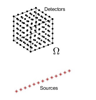
Figure 1: A schematic diagram measurements.

5.1.1 The forward problem of TTTP (1.4)

We solve the forward problem to generate the data of the arriving time $g\left(\mathbf{x},\mathbf{x}_{0}\right)=\tau\left(\mathbf{x},\mathbf{x}_{0}\right)$ in (1.4) for TTTP of section 1 as follows. Given the heterogeneous medium $m(\mathbf{x})$, instead of solving the nonlinear eikonal equation (1.2) and (1.3) directly, we have solved the forward problem (1.2)-(1.3) for each of those 101 sources located on $L_{src}$ by the 3D fast marching method built in Matlab. The Fast Marching method is a technique that approximates the solution of the Eikonal nonlinear partial differential equation, it is similar to the Dijkstra algorithm to find the shortest paths in graphs which are uniformly sized spatial grid with sound speed value at each node. For each source located on $L_{src}$, the Fast Marching method simultaneously computes the shortest paths $\Gamma(\mathbf{x},\mathbf{x}_{0})$ on graphs and the arriving time $\tau(\mathbf{x},\mathbf{x}_{0})$. Here we set the step size with respect to spatial variables for the fast marching method $h_{\text{sp}}=1/30$.

5.1.2 The inverse problem

Having the computationally simulated data (1.4) for the inverse problem, which are computed as in sub-subsection 5.1.1, we add the random noise to these data as:

$$g_{\text{noise}}\left(\mathbf{x},\mathbf{x}_{0}\right)=g\left(\mathbf{x},\mathbf{x}_{0}\right)+\delta\max_{\mathbf{x}\in\partial\Omega,\mathbf{x}_{0}\in L_{\text{src}}}|g\left(\mathbf{x},\mathbf{x}_{0}\right)|\xi_{\mathbf{x}_{0}},\text{ }\mathbf{x}\in\partial\Omega,\mathbf{x}_{0}\in L_{\text{src}},$$

Here $\xi_{\mathbf{x}_{0}}\in\left(-1,1\right)$ is the uniformly distributed random variable and $\delta=0.05$, i.e. $5\%$ noise level in all the numerical tests.

To solve inverse problem (1.4) numerically, we have first selected optimal values for some parameters. Those values were selected by the trial and error procedure. We show below the effects of different combinations of these parameters in the first two tests. As soon as the best parameters were selected in the first two tests, they were used in the rest of tests.

We have solved the following minimization problem:

Minimization Problem. Minimize the functional

$$J_{\lambda,\beta}\left(W^{h}\right)=\left\|\left[M_{N}W^{h}+P\left(W_{x}^{h},W_{y}^{h},g_{x}^{h},g_{y}^{h},\mathbf{x}^{h}\right)\right]e^{\lambda z}\right\|_{L_{2,N}^{h}\left(\Omega^{h}\right)}^{2}+\beta\left\|W^{h}\right\|_{H_{N}^{2,h}\left(\Omega^{h}\right)}^{2},$$ (5.1)

on the set $\overline{K^{h}\left(R\right)}$ defined in (2.44), where $\beta\in\left(0,1\right)$ is the regularization parameter.

Here the space $H_{N}^{2,h}\left(\Omega^{h}\right)$ is defined as

$$H_{N}^{2,h}\left(\Omega^{h}\right)=\left\{\begin{array}[]{c}Q^{h}(\mathbf{x}^{h}):\left\|Q^{h}\right\|_{H_{N}^{2,h}\left(\Omega^{h}\right)}^{2}=\\ \left\|Q_{x}^{h}\right\|_{L_{2N}^{h}\left(\Omega^{h}\right)}^{2}+\left\|Q_{y}^{h}\right\|_{L_{2N}^{h}\left(\Omega^{h}\right)}^{2}+\mathop{\displaystyle\sum}\limits_{s=0}^{2}\left\|\partial_{z}^{s}Q^{h}\right\|_{L_{2N}^{h}\left(\Omega^{h}\right)}^{2}<\infty\end{array}\right\}.$$

The regularization term $\beta\left\|W^{h}\right\|_{H_{N}^{2,h}\left(\Omega^{h}\right)}^{2}$ in (5.1) is not involved in our above theory. On the other hand, we see in our numerical experiments that our method does not perform well without the regularization term. We cannot explain yet why this takes place, and this should be a subject of our further research. We note that since the regularization term represents a strictly convex functional $Y_{\beta}:H_{N}^{2,h}\left(\Omega^{h}\right)\rightarrow\mathbb{R},$

$$Y_{\beta}\left(W^{h}\right)=\beta\left\|W^{h}\right\|_{H_{N}^{2,h}\left(\Omega^{h}\right)}^{2},$$

then an obvious analog of Theorem 3.1 implies that the functional $J_{\lambda,\beta}\left(W^{h}\right):K_{2}^{h}\left(R\right)\rightarrow\mathbb{R}$ is strictly convex on the set $\overline{K_{2}^{h}\left(R\right)},$ where $K_{2}^{h}\left(R\right)$ is obtained from the set $K^{h}\left(R\right)$ in (2.44) via replacing in (2.44) $H_{N}^{1,h}\left(\Omega^{h}\right)$ with $H_{N}^{2,h}\left(\Omega^{h}\right).$ Then (3.3) should be replaced with

$$J_{\lambda,\beta}\left(W_{2}^{h}\right)-J_{\lambda,\beta}\left(W_{1}^{h}\right)-J_{\lambda,\beta}^{\prime}\left(W_{1}^{h}\right)\left(W_{2}^{h}-W_{1}^{h}\right)\geq$$

$$\geq C\left\|W_{2}^{h}-W_{1}^{h}\right\|_{H_{2,N}^{1,h}\left(\Omega^{h}\right)}^{2}+\beta\left\|W_{2}^{h}-W_{1}^{h}\right\|_{H_{2,N}^{2,h}\left(\Omega^{h}\right)}^{2},\forall W_{1}^{h},W_{2}^{h}\in\overline{K_{2}^{h}\left(R\right)}.$$

We have minimized the fully discrete version of $J_{\lambda,\beta}\left(W^{h}\right)$ with respect to the values of the corresponding vector function at grid points. To minimize the discretized functional $J_{\lambda,\beta}\left(W^{h}\right)$, we use the Matlab’s built-in function fminunc to solve the optimization problem. This function calculates the gradient $\nabla J_{\lambda,\beta}\left(W^{h}\right)$ automatically, and we let the iterations stop when the condition $|\nabla J_{\lambda,\beta}\left(W^{h}\right)|<10^{-6}$ is fulfilled.

5.2 Results

In the numerical tests of this subsection, we demonstrate the efficiency of our method. We display on Figures the true and computed functions $n\left(\mathbf{x}\right)=\sqrt{m\left(\mathbf{x}\right)}$, see section 1. In all tests the background value $n_{\text{bkgr}}\left(\mathbf{x}\right)=1$, which corresponds to the background value $c_{\text{bkgr}}\left(\mathbf{x}\right)=1.$ In those figures below, we depict 2-D slices to demonstrate the values of the true function $n\left(\mathbf{x}\right)$ and computed function $n_{\text{comp}}\left(\mathbf{x}\right)$.

We have chosen values of all our parameters by the trial and error procedure. In all tests, we set the regularization parameter in (5.1) $\beta=10^{-4}.$ In the first two tests, we use the mesh step size $h=1/10$. And for the tests number 3-5, we use the mesh step size $h=1/15$ for better resolutions. In Tests 1 and 2 we select an optimal pair $\left(\lambda,N\right)$ of parameters. Therefore, we work in the first two tests with a ball-shaped inclusion which is a rather simple shape. As soon as an optimal pair $\left(\lambda,N\right)$ is selected, we work in Tests 3-5 with letter-like shapes of inclusions. We have chosen letters since they are non convex and have voids, i.e. their shapes are rather complicated ones.

Test 1. First, we test the reconstruction by our method of the case of a ball-shaped inclusion. The true function $n(\mathbf{x})$ is depicted on Figures 2 (a) and (b), $n(\mathbf{x})=1.5$ inside of this inclusion and $n(\mathbf{x})=1$ outside of it. Since $m(\mathbf{x})=1.5^{2}$ inside of this inclusion and $m(\mathbf{x})=1$ outside of it, then the inclusion/background contrast in the target function $m(\mathbf{x})$ is $1.5^{2}:1=2.25:1.$ In this test, we fix $N=6$ and vary $\lambda$ from 0 to 4. See Figures 2 for the reconstruction results. One can observe that the result with $\lambda=0$ i.e. in the case when the Carleman Weight Function is absent in the functional $J_{\lambda,\rho}\left(W^{h}\right),$ is unacceptable. Even though results with $\lambda=2,3,4$ are about the same, we choose $\lambda=4$ as the optimal value since our theory basically says that larger values of $\lambda$ are better than lower ones.

Test 2. In this case, we test the influence of the parameter $N$. We again use the same inclusion as the one in Test 1. We fix the parameter $\lambda=4,$ which we have chosen in Test 1, and allow $N$ to vary from 4 to 10. See Figures 3 for the results of the reconstruction. One can observe that the reconstruction results for $N=6,8,10$ are basically the same. Therefore, we choose $N=6$ since this choice ensures a lesser computational cost.

In conclusion, we select an optimal pair $\left(\lambda,N\right)$ of parameters as:

$$\lambda=4,N=6\text{ in tests }3-5.$$ (5.2)

In tests 3-5 inclusions are letter-shaped. We have intentionally chosen these shapes since they are non convex and are, therefore, hard to image.

Test 3. We test the reconstruction by our method of the case when the shape of our inclusion is the same as the shape of the letter ‘$A$’. The function $n(\mathbf{x})$ is depicted on Figures 4 (a) and (b). $n=1.5$ inside of this inclusion and $n=1$ outside of it. See Figures 4 for the reconstruction results.

Test 4. We test the reconstruction by our method for the case when the shape of our inclusion is the same as the shape of the letter ‘$C$’. The function $n(\mathbf{x})$ is depicted on Figures 5 (a) and (b). $n=1.5$ inside of this inclusion and $n=1$ outside of it. See Figures 5 for the reconstruction results.

Test 5. We test the reconstruction by our method of the case when the shape of our inclusion is the same as the shape of the letter ‘$\Omega$’. The function $n(\mathbf{x})$ is depicted on Figures 6 (a) and (b). $n=1.5$ inside of this inclusion and $n=1$ outside of it. See Figures 6 for the reconstruction results.

6 Summary

We have presented the first computational result for the Travel Time Tomography Problem in the 3-D case. To do this, we have implemented numerically the version of [22], [26, Chapter 11] of the globally convergent convexification numerical method. This method minimizes a certain weighted cost functional with the Carleman Weight Function in it. We have provided the global convergence analysis for our method. Interestingly our computations for Test 1 with $\lambda=0$ show that results have an unacceptable quality when the Carleman Weight Function is absent in this functional. We have imaged letter-shaped inclusions, which are non convex and are, therefore, hard to image. Nevertheless, shapes of inclusions are imaged accurately in all tests.

The true inclusion/background contrast in the target function $m\left(\mathbf{x}\right)$ is 2.25:1 in all tests. On the other hand, it follows from Figures 2-6 that the computed contrasts vary between $1.3^{2}:1=1.69:1$ and $1.4^{2}:1=1.96:1.$ Also, some other refinements of our results are desirable. We hope to obtain them in the future.

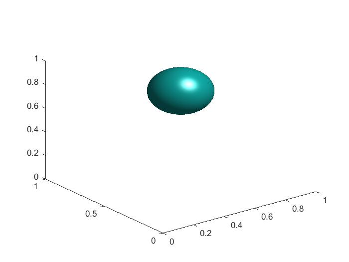
(a) Slice image of the true $n$	(b) 3D image of the true $n$
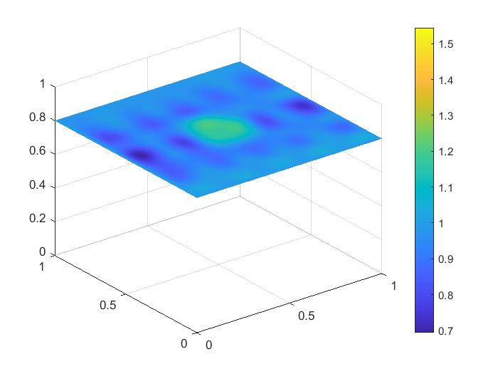
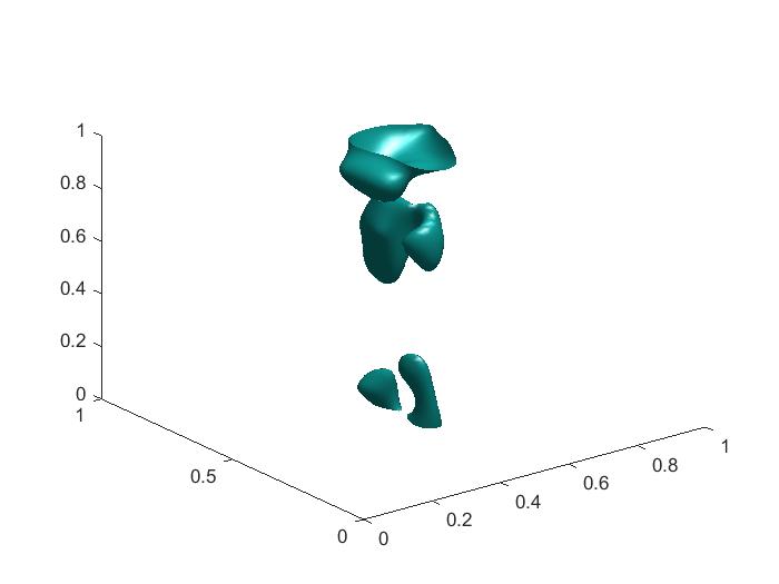
(c) Slice image of $n_{comp}$ for $\lambda=0$	(d) 3D image of $n_{comp}$ for $\lambda=0$
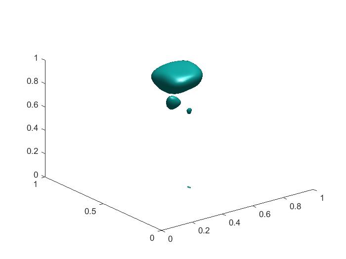
(e) Slice image of $n_{comp}$ for $\lambda=1$	(f) 3D image of $n_{comp}$ for $\lambda=1$
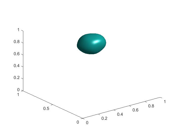
(g) Slice image of $n_{comp}$ for $\lambda=2$	(h) 3D image of $n_{comp}$ for $\lambda=2$
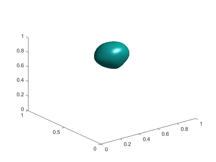
(i) Slice image of $n_{comp}$ for $\lambda=3$	(j) 3D image of $n_{comp}$ for $\lambda=3$
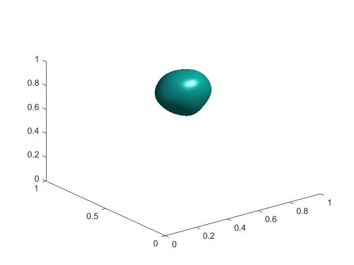
(k) Slice image of $n_{comp}$ for $\lambda=4$	(l) 3D image of $n_{comp}$ for $\lambda=4$

Figure 2: Results of Test 1. We test the effects of the parameter $\lambda$. In this test, we fix $N=6$ and $\lambda$ varies from 0 to 4.

(a)Slice image of the true $n$	(b) 3D image of the true $n$
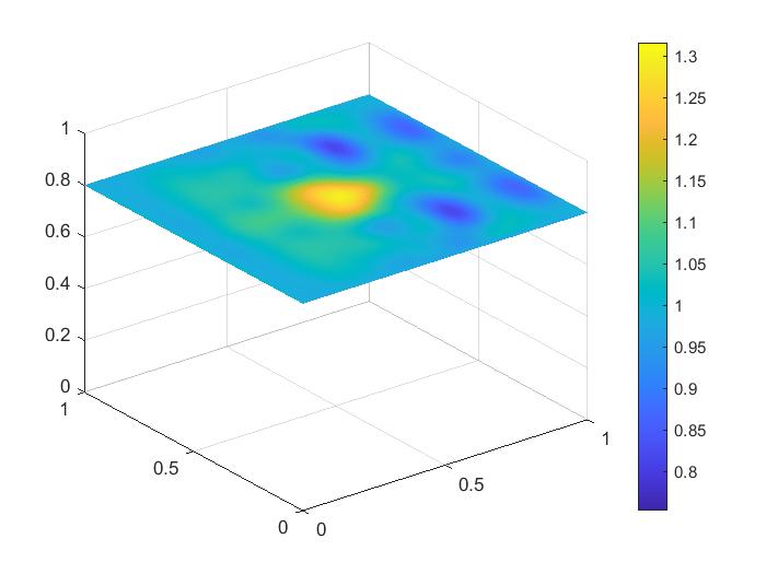
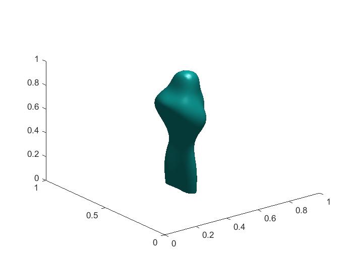
(c) Slice image of $n_{comp}$ for $N=4$	(d) 3D image of $n_{comp}$ for $N=4$
(e) Slice image of $n_{comp}$ for $N=6$	(f) 3D image of $n_{comp}$ for $N=6$
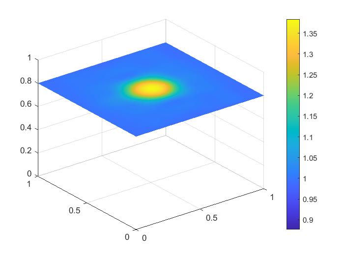
(g) Slice image of $n_{comp}$ for $N=8$	(h) 3D image of $n_{comp}$ for $N=8$
(i) Slice image of $n_{comp}$ for $N=10$	(j) 3D image of $n_{comp}$ for $N=10$

Figure 3: Results of Test 2. We test the effects of the parameter $N$. Here we fix the parameter $\lambda=4$ and $N$ varies from 4 to 10.

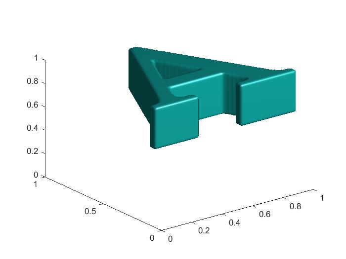
(a) Slice image of the true $n$	(b) 3D image of the true $n$
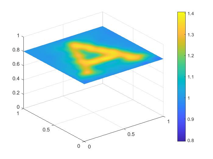
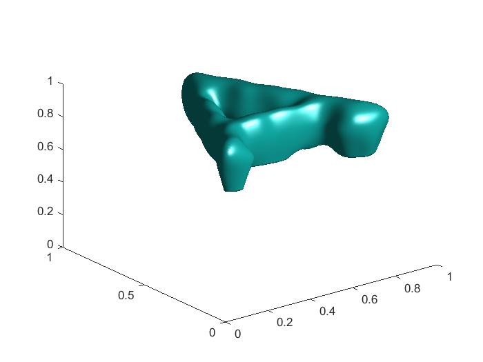
(c) Slice image of $n_{comp}$	(d) 3D image of $n_{comp}$

Figure 4: Results of Test 3. Imaging of ‘A’ shaped $n$ with $n=1.5$ in it and $n=1$ outside. In this example, we set the parameter $N=6$ and $\lambda=4$, see (5.2).

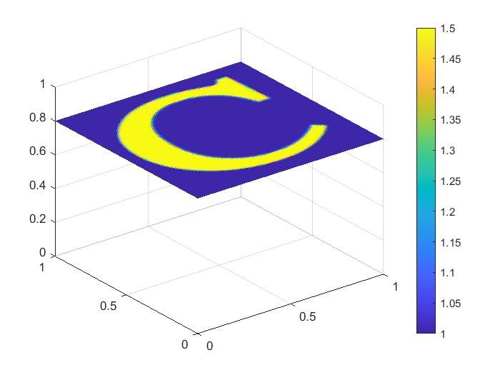
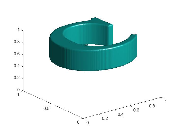
(a) Slice image of the true $n$	(b) 3D image of the true $n$
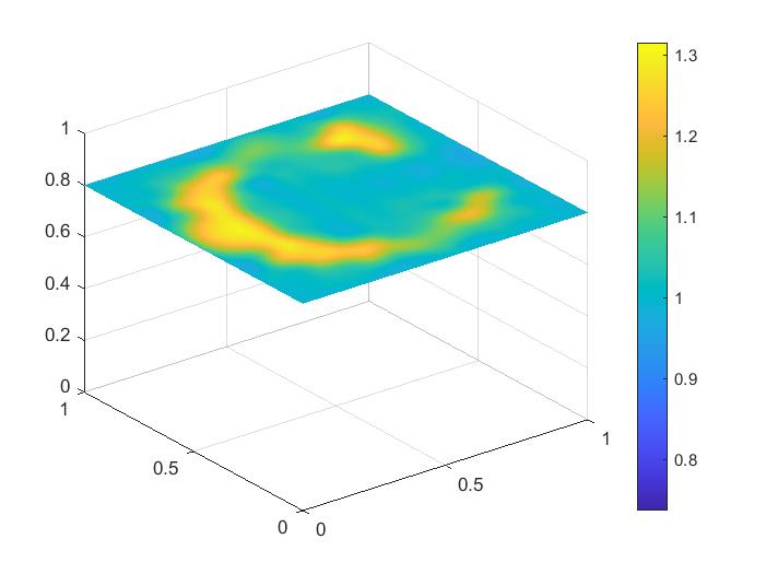
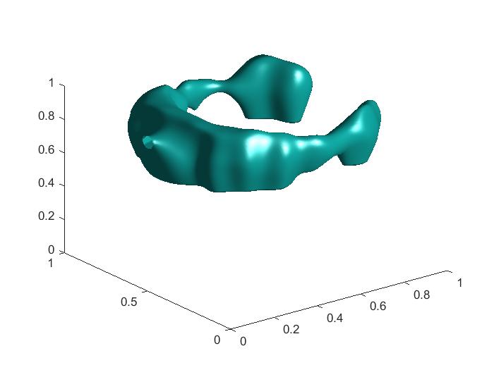
(c) Slice image of $n_{comp}$	(d) 3D image of $n_{comp}$

Figure 5: Results of Test 4. Imaging of ‘C’ shaped $n$ with $n=1.5$ in it and $n=1$ outside. In this example, we set the parameter $N=6$ and $\lambda=4$, see (5.2).

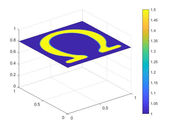
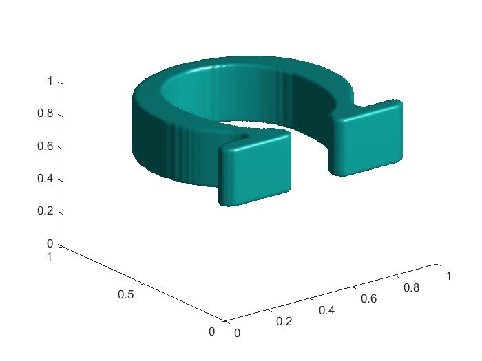
(a) Slice image of the true $n$	(b) 3D image of the true $n$
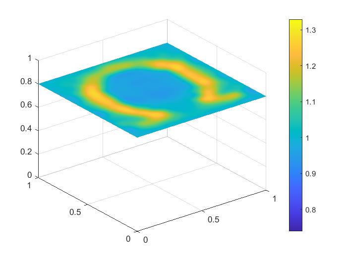
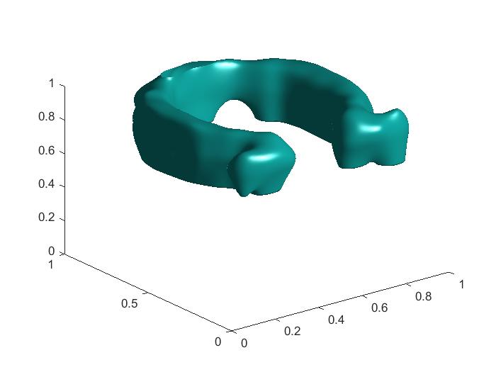
(c) Slice image of $n_{comp}$	(d) 3D image of $n_{comp}$

Figure 6: Results of Test 5. Imaging of ‘ $\Omega$’ shaped $n$ with $n=1.5$ in it and $n=1$ outside. In this example, we set the parameter $N=6$ and $\lambda=4$, see (5.2).

CRediT Authorship Contribution Statement

1. Michael V. Klibanov: Conceptualization, Methodology, Formal Analysis, Supervision, Writing – original draft, Writing – review & editing.

2. Jingzhi Li: Conceptualization, Methodology, Supervision, Writing – original draft, Writing – review & editing.

3. Wenlong Zhang: Conceptualization, Investigation, Software, Validation, Visualization, Writing – review & editing

7 Declaration of competing interest

The authors declare that they have no known competing financial interests or personal relationships that could have appeared to influence the work reported in this paper.

References

• [1] A.B.Β Bakushinskii, M.V. Klibanov and N.A. Koshev, Carleman weight functions for a globally convergent numerical method for ill-posed Cauchy problems for some quasilinear PDEs, Nonlinear Analysis: Real World Applications, 34 (2017), 201-224.
• [2] L. Beilina and M.V. Klibanov, Approximate global convergence and adaptivity for coefficient inverse problems, Springer, New York, 2012.
• [3] M. Bellassoued and M. Yamamoto, Carleman estimates and applications to inverse problems for hyperbolic systems, Springer Japan KK, 2017.
• [4] M.Β Born and E.Β Wolf, Principles of optics, 7th ed., Cambridge University Press, 1999.
• [5] A. L. Bukhgeim and M. V. Klibanov, Uniqueness in the large of a class of multidimensional inverse problems, Soviet Math. Doklady, 17 (1981), 244–247.
• [6] G. Chavent, Nonlinear least squares for inverse problems: theoretical foundations and step-by-step guide for applications, Berlin: Springer Science & Business Media, 2010.
• [7] A. V. Goncharsky and S. Y. Romanov, Iterative methods for solving coefficient inverse problems of wave tomography in models with attenuation, Inverse Problems, 33 (2017), 025003.
• [8] A. V. Goncharsky and S. Y. Romanov, A method of solving the coefficient inverse problems of wave tomography, Computers and Mathematics with Applications, 77 (2019), 967–980.
• [9] J.P. Guillement and R.Β G. Novikov, Inversion of weighted Radon transforms via finite Fourier series weight approximation, Inverse Problems in Science and Engineering, 22 (2013), 787–802.
• [10] G.Β Herglotz, Ε°ber die Elastizitaet der Erde bei Beruecksichtigung ihrer variablen Dichte, Zeitschr. fur Math. Phys., 52 (1905), 275-299.
• [11] V. Isakov, Inverse problems for partial differential equations, Second Edition, Springer, New York, 2006.
• [12] S.Β I. Kabanikhin, K.Β K. Sabelfeld, N.Β S. Novikov, and M.Β A. Shishlenin, Numerical solution of the multidimensional Gelfand-Levitan equation, J. Inverse and Ill-Posed Problems, 23 (2015), 439–450.
• [13] V. A. Khoa, G. W. Bidney, M. V. Klibanov, Loc H. Nguyen, Lam H. Nguyen, A. J. Sullivan and V. N. Astratov, Convexification and experimental data for a 3D inverse scattering problem with the moving point source, Inverse Problems, 36 (2020), 085007.
• [14] M. V. Klibanov, Inverse problems in the β€˜large’ and Carleman bounds, Differential Equations, 20 (1984), 755–760.
• [15] M. V. Klibanov, Inverse problems and Carleman estimates, Inverse Problems, 8 (1992), 575–596.
• [16] M. V. Klibanov and O. V. Ioussoupova, Uniform strict convexity of a cost functional for three-dimensional inverse scattering problem, SIAM J. Math. Anal., 26 (1995), 147–179.
• [17] M.V. Klibanov, Global convexity in a three-dimensional inverse acoustic problem SIAM J. Mathematical Analysis, 28 (1997), 1371-1388.
• [18] M.Β V. Klibanov, Carleman estimates for global uniqueness, stability and numerical methods for coefficient inverse problems, J. Inverse and Ill-Posed Problems, 21 (2013), Β 477–560.
• [19] M.V. Klibanov and V.G. Romanov, Reconstruction procedures for two inverse scattering problems without the phase information, SIAM J. Appl. Math., 76 (2016), pp. 178-196.
• [20] M.V. Klibanov, Convexification of restricted Dirichlet-to-Neumann map, J. Inverse and Ill-Posed Problems, 25 (2017), 669-685.
• [21] M.Β V. Klibanov, J. Li and W. Zhang,Β Electrical impedance tomography with restricted Dirichlet-to-Neumann map data, Inverse Problems, 35 (2019), 035005.
• [22] M. V. Klibanov, Travel time tomography with formally determined incomplete data in 3D, Inverse Problems and Imaging, 13 (2019), 1367–1393.
• [23] M. V. Klibanov, On the travel time tomography problem in 3D, J. Inverse Ill-Posed Probl., 27 (2019), 591–607.
• [24] M. V. Klibanov, T.T. Le and L.H. Nguyen, Numerical solution of a linearized travel time tomography problem with incomplete data, SIAM J. Scientific Computing, 42 (2020), B1173-B1192.
• [25] M.V. Klibanov, J. Li and W. Zhang, Convexification for an inverse parabolic problem, Inverse Problems, 36 (2020), 085008.
• [26] M.Β V.Β Klibanov and J. Li, Inverse problems and Carleman estimates: global uniqueness, global convergence and experimental data, De Gruyter, 2021.
• [27] M.V. Klibanov, A.V. Smirnov, V.A. Khoa, A.J. Sullivan and L.H. Nguyen, Through-the-wall nonlinear SAR imaging, IEEE Transactions on Geoscience and Remote Sensing, 59 (2021), 7475-7486.
• [28] M.Β V. Klibanov, V.Β A. Khoa, A.Β V. Smirnov, L.Β H. Nguyen, G.Β W. Bidney, L.Β Nguyen, A.Β Sullivan, and V.Β N. Astratov, Convexification inversion method for nonlinear SAR imaging with experimentally collected data, Journal of Applied and Industrial Mathematics, 15 (2021), 413–436.
• [29] M.V. Klibanov, J. Li and Z. Yang, Convexification numerical method for a coefficient inverse problem for the radiative transport equation, arXiv: 2206.11675, 2022.
• [30] M.M. Lavrentiev, V.G. Romanov and S.P. Shishatskii, Ill-posed problems of mathematical physics and analysis, AMS, Providence: RI, 1986.
• [31] V.G. Romanov, Inverse problems of mathematical physics, VNU Press, Utrecht, 1986.
• [32] Β J.A. Scales, M.L. Smith and T.L. Fischer, Global optimization methods for multimodal inverse problems, J. Comp. Phys., 103 (1992), 258–268.
• [33] U. SchrΕ‘der and T. Schuster, An iterative method to reconstruct the refractive index of a medium from time-off-light measurements, Inverse Problems, 32 (2016), 085009.
• [34] A.N. Tikhonov, A.V. Goncharsky, V.V. Stepanov and A.G. Yagola, Numerical methods for the solution of ill-posed problems, Kluwer, London, 1995.
• [35] M.M. Vajnberg, Variational method and method of monotone operators in the theory of nonlinear equations, John Wiley& Sons, Washington, DC, 1973.
• [36] L. Volgyesi and M. Moser, The inner structure of the Earth, Periodica Polytechnica Chemical Engineering, 26 (1982), 155-204.
• [37] E. Wiechert and K. Zoeppritz, Uber Erdbebenwellen, Nachr. Koenigl. Geselschaft Wiss. Gottingen, 4 (1907), 415-549.
• [38] H. Zhao and Y. Zhong, A hybrid adaptive phase space method for reflection traveltime tomography, SIAM J. Imaging Sciences, 12 (2019), 28-53.
• [39] M.Β Yamamoto,Β Carleman estimates for parabolic equations. Topical Review, Inverse Problems, 25 (2009), 123013.