Machine Learning for Bilevel and Stochastic Programming

A Machine Learning Approach to Solving Large Bilevel and Stochastic Programs: Application to Cycling Network Design

Timothy C. Y. Chan, Bo Lin Department of Mechanical & Industrial Engineering, University of Toronto, {tcychan, blin}@mie.utoronto.ca, Shoshanna Saxe Department of Civil & Mineral Engineering, University of Toronto, s.saxe@utoronto.ca,

We present a novel machine learning-based approach to solving bilevel programs that involve a large number of independent followers, which as a special case include two-stage stochastic programming. We propose an optimization model that explicitly considers a sampled subset of followers and exploits a machine learning model to estimate the objective values of unsampled followers. Unlike existing approaches, we embed machine learning model training into the optimization problem, which allows us to employ general follower features that can not be represented using leader decisions. We prove bounds on the optimality gap of the generated leader decision as measured by the original objective function that considers the full follower set. We then develop follower sampling algorithms to tighten the bounds and a representation learning approach to learn follower features, which can be used as inputs to the embedded machine learning model. Using synthetic instances of a cycling network design problem, we compare the computational performance of our approach versus baseline methods. Our approach provides more accurate predictions for follower objective values, and more importantly, generates leader decisions of higher quality. Finally, we perform a real-world case study on cycling infrastructure planning, where we apply our approach to solve a network design problem with over one million followers. Our approach presents favorable performance compared to the current cycling network expansion practices.

bilevel optimization; two-stage stochastic programming; machine learning; model reduction; cycling network design.

1 Introduction

This paper is concerned with solving bilevel optimization problems with a large number of followers and where the feasible region of the leader is independent of the followers. A wide range of decision problems can be modeled this way, including active transportation network design (Liu et al. 2019, 2022a, Lim et al. 2021), network pricing (Van Hoesel 2008, Alizadeh et al. 2013), energy pricing (Fampa et al. 2008, Zugno et al. 2013), and portfolio optimization (Carrión et al. 2009, Leal et al. 2020). This model also generalizes two-stage stochastic programming. Indeed, if the objectives of the leader and followers are identical, then this model becomes a two-stage stochastic program where the followers represent scenarios. Thus, in this paper, the reader should think of “leader” in a bilevel program and “first-stage decision maker” in a stochastic program as synonymous, and similarly for “follower” and “second-stage decision maker”. As we discuss the bilevel or stochastic programming literature below, we use the corresponding terminology.

Having a large set of followers $\mathcal{S}$ adds to the difficult task of solving a bilevel problem by increasing the problem size. For the bilevel problem we consider, given its relationship to stochastic programming, we can draw on approaches to deal with large $\mathcal{S}$ from both communities. Two predominant strategies are: i) solving the problem with a small sample of $\mathcal{S}$, and ii) approximating follower costs without solving the follower problems.

Sampling a smaller follower set can be done via random sampling (Liu et al. 2022a, Lim et al. 2021) or clustering (Dupačová et al. 2003, Hewitt et al. 2021, Bertsimas and Mundru 2023). Given a sample $\mathcal{T}\subseteq\mathcal{S}$, we can obtain a feasible leader solution by solving the reduced problem, which improves computational tractability and solution interpretability due to the reduced problem size. Furthermore, under suitable regularity assumptions, an optimal solution to the reduced problem provides a bound on the optimal value and optimal leader solution to the original problem (Römisch and Schultz 1991, Römisch and Wets 2007). However, there is no theoretical guarantee on the performance of the optimal solution to the reduced problem as measured by the original problem’s objective.

Regarding the second strategy, many different algorithms have been developed to approximate the followers’ cost. Such approximations can be obtained by relaxing the constraint that the followers’ decisions are optimal for their own objectives and progressively refining the relaxed problem until the generated follower solutions are optimal. Refinement typically involves iteratively solving the followers’ problems, which can be accelerated through parallelization. Algorithms along this direction include L-shaped methods (Birge and Louveaux 2011), vertex enumeration (Candler and Townsley 1982), the Kuhn-Tucker approach (Bard 2013), and penalty function methods (White and Anandalingam 1993). However, these algorithms are generally not able to deal with huge $\mathcal{S}$ because i) the refinement process can take a large number of iterations to converge and ii) the relaxed problem size still increases as $|\mathcal{S}|$ increases, which is particularly problematic when the leader’s problem is hard, for example, when it is non-convex. To overcome this issue, machine learning (ML) and continuous approximation methods have recently achieved encouraging performance on approximating the second-stage cost as a function of first-stage decisions (Carlsson 2012, Liu et al. 2021, Stroh et al. 2022, Patel et al. 2022) and learning second-stage decision rules (Chen et al. 2008). However, the former requires identifying features that can be compactly represented using the leader’s decision, which is practically challenging, while the latter may produce infeasible decisions when nontrivial second-stage constraints are present. Moreover, neither method has optimality guarantees.

In this paper, we build on the ideas from both strategies. In particular, we consider sampling a subset $\mathcal{T}\subseteq\mathcal{S}$. However, we also augment the overall objective function with an estimate of the objective value of the unsampled followers, from $\mathcal{S}\backslash\mathcal{T}$, using an ML model. Unlike existing methods that use offline ML models to map leader decisions to objective values, our ML model takes follower features that are independent of leader decisions. We embed the ML model training into the bilevel problem to link the ML model with leader decisions. When optimizing leader decisions, the ML model is trained on a dataset of the sampled followers on-the-fly. Simultaneous optimization and ML model training enables derivation of new theoretical guarantees for the generated leader decisions. Finally, to demonstrate our methodology, we apply it to a cycling infrastructure design problem, completed in collaboration with the City of Toronto using real data. The methods we develop in this paper were driven by the need to solve this large, real-world application.

1.1 Problem Motivation: Cycling Infrastructure Planning

Cycling has become an increasingly popular transportation mode due to its positive impact on urban mobility, public health, and the environment (Mueller et al. 2018, Kou et al. 2020) In fact, during the COVID-19 pandemic, cycling popularity increased significantly since it represented a low-cost and safe alternative to driving and public transit, facilitated outdoor activities, and improved access to essential services (Kraus and Koch 2021, Buehler and Pucher 2021). However, cycling safety and comfort concerns have been repeatedly identified as major factors that inhibit cycling uptake and overall mode choice (Dill and McNeil 2016, Li et al. 2017). Building high-quality cycling infrastructure is among the most effective ways to alleviate cycling stress and enhance cycling adoption (Buehler and Dill 2016). In this paper, we develop a bilevel optimization model to optimize cycling infrastructure network design. The model maximizes “low-stress cycling accessibility” subject to a fixed budget. Low-stress cycling accessibility, defined as the total amount of “opportunities” (i.e., people, jobs, retail stores) reachable by individuals using streets that are safe for cycling, has been widely adopted to assess the service provided by transportation infrastructure and the impact of cycling infrastructure (Sisson et al. 2006, Lowry et al. 2012, Furth et al. 2018, Kent and Karner 2019, Imani et al. 2019, Gehrke et al. 2020, Lin et al. 2021). The leader is a transportation planner who designs a cycling network subject to a given budget, considering that cyclists will use the low-stress network to travel to opportunities via shortest paths. The followers are cyclists. Since the planner’s objective is to maximize the total number of opportunities accessible via low-stress routes, the followers correspond to all possible origin-destination pairs between units of population and opportunity. The resulting formulation for the City of Toronto includes over one million origin-destination pairs between 3,702 small geographic units known as census dissemination areas (DAs) (Statistics Canada 2016a), motivating the development of our methodology.

1.2 Contributions

1. We develop a novel ML-augmented optimization model for solving bilevel optimization problems with a large number of followers. Our objective function has an exact component for a sampled subset of followers and an approximate component derived from an ML model. Sampling improves computational tractability, while the ML model ensures that the objective function better captures the impact of the leader’s decision on the unsampled followers. The training of the ML model is embedded into the optimization model to enable the use of predictive features that cannot be compactly represented using leader decisions. We consider both parametric and non-parametric ML models, and develop corresponding theoretical bounds on the quality of the generated solution as measured on the original objective function with the full set of followers. Given that this model generalizes two-stage stochastic programming, our ML-augmented approach also represents a new way for solving stochastic programming problems.

2. Informed by our theoretical insights, we develop practical strategies to enhance the performance of the ML-augmented model, including i) follower sampling algorithms to tighten the theoretical bounds, ii) strategies for hyperparameter tuning, and iii) a novel representation learning framework that automatically learns follower features that are predictive of follower objective values. To the best of our knowledge, this is the first application of representation learning to bilevel optimization.

3. We demonstrate the effectiveness of our approach via computational studies on a synthetic cycling network design problem. We show that i) our learned features are more predictive of follower objective values compared to baseline features from the literature; ii) our follower sampling algorithms further improve the ML models’ out-of-sample prediction accuracy by a large margin compared to baseline sampling methods; iii) our strong predictive performance translates into high-quality and stable leader decisions from the ML-augmented model. The performance gap between our approach and sampling-based models without the ML component is particularly large when the follower sample is small.

4. In collaboration with the City of Toronto, we perform a real-world case study on cycling infrastructure planning in Toronto, Canada. We solve a large-scale cycling network design problem where we compare our model against i) purely sampling-based methods that do not use ML and ii) a greedy expansion method that closely matches real-world practice. Compared to i), our method can achieve accessibility improvements between 5.8–34.3%. Compared to ii), our approach can further increase accessibility by 19.2% on average. If we consider 100 km of cycling infrastructure to be designed using a greedy method, our method can achieve a similar level of accessibility using only 70 km, equivalent to $18M in potential cost savings, or an 11.2% increase in accessibility if all 100 km was designed using our approach.

All proofs are in the Electronic Companion.

2 Literature review

2.1 Integration of Machine Learning and Optimization

There has been tremendous growth in the combination of ML and optimization techniques. Traditional “predict, then optimize” is a common modeling paradigm that uses machine learning models to estimate parameters in an optimization problem, which is then solved with those estimates to obtain decisions (Ferreira et al. 2016, Elmachtoub and Grigas 2022). Recent progress has been made in using ML models to prescribe decisions based on contextual features (Ban and Rudin 2019, Notz and Pibernik 2022, Babier et al. 2023, Bertsimas and Kallus 2020), and to build end-to-end optimization solvers (Vinyals et al. 2015, Bello et al. 2017, Khalil et al. 2017, Nazari et al. 2018, Kool et al. 2019). Machine learning is also used to speed-up optimization algorithms such as branch and bound (Khalil et al. 2016), cutting planes (Tang et al. 2020, Jia and Shen 2021), column generation (Morabit et al. 2021), and meta-heuristics (Song et al. 2020) (See Bengio et al. (2021) and Kotary et al. (2021) for comprehensive reviews.). Closest to our work is a stream of literature that integrates offline ML models into the solution of optimization problems to map decision variables to uncertain objective values (Biggs et al. 2017, Mišić 2020, Liu et al. 2021, Bergman et al. 2022, Patel et al. 2022). Our work differs in that we integrate the ML model training directly into the optimization problem and use predictive features that cannot be compactly represented using our decision variables.

2.2 Scenario Reduction in Stochastic Programming

Scenario reduction has been extensively studied in the stochastic programming literature. One stream of literature quantifies the similarity between individual scenarios and then applies clustering methods to select a subset. Common measures include the cost difference between single-scenario optimization problems (Keutchayan et al. 2023), the opportunity cost of switching between scenarios (Hewitt et al. 2021), and the distance between scenario feature vectors (Crainic et al. 2014, Wu et al. 2022). Another stream of literature selects a scenario subset from a given set to minimize the discrepancy between the distributions described by the two sets. Probabilistic metrics, including Wasserstein distance (Römisch and Schultz 1991, Bertsimas and Mundru 2023) and Fortet-Mourier metrics (Dupačová et al. 2003), derived from the stability theory of stochastic programming, and heuristic loss functions (Prochazka and Wallace 2020) have been proposed to measure such discrepancies.

Our proposal of learning follower representations is similar to Wu et al. (2022). However, our approach does not rely on the graph structure of the optimization problem and considers the impact of the leader’s solution on the followers’ costs. Our theoretical results differ from the traditional scenario reduction literature in that instead of focusing on the stability of the optimal value and optimal leader’s solution, we provide solution quality guarantees for the leader’s solution obtained from solving our ML-augmented problem. More recently, Zhang et al. (2023) proved a similar bound assuming that the second-stage cost is Lipschitz in the first-stage decision. In contrast, our bounds do not require this assumption and enjoy tightness guarantees which was not considered in the previous literature.

2.3 Active Learning

Active learning aims to reduce the cost of data labeling by selecting the most “informative” subset of data for machine learning model training. Such a subset is typically constructed through an iterative process where an ML model is trained on the labeled data at each iteration and then queries one or more unlabeled data points based on informativeness measures such as prediction uncertainty (Lewis and Gale 1994), and expected model change (Settles et al. 2007). See Settles (2009) for a comprehensive review of the available measures. Instead of iteratively selecting unlabeled data, a subset of data may be selected once to improve data labeling efficiency (Sener and Savarese 2018). Our approach is most similar to Sener and Savarese (2018) because including the exact objective for a sampled set of followers in the reduced problem is analogous to costly labeling of a small set of data points once. We extend the core-set method developed by Sener and Savarese (2018) to derive a theoretical bound for the quality of the leader decisions from our ML-augmented model.

2.4 Strategic Cycling Infrastructure Planning

Previous studies on strategic cycling infrastructure planning have considered a variety of approaches. Many papers greedily choose road segments to install new cycling infrastructure using expert-defined metrics (Lowry et al. 2012, Kent and Karner 2019, Olmos et al. 2020) or visualization techniques (Larsen et al. 2013, Putta and Furth 2019). Optimization-based approaches typically consider minimizing the travel cost (Sohn 2011, Mesbah et al. 2012, Duthie and Unnikrishnan 2014, Bagloee et al. 2016, Mauttone et al. 2017), maximizing total utility (Bao et al. 2017, Liu et al. 2019, 2022a, Lim et al. 2021, Ospina et al. 2022), or maximizing total ridership (Liu et al. 2022b) given a large number of origin-destination (OD) pairs. Due to the large problem size, such models are usually solved with heuristics. To the best of our knowledge, only Liu et al. (2022a), Lim et al. (2021), and Liu et al. (2022b) solve the problems to optimality at a city scale by randomly sampling OD pairs or restricting the routes that can be used by each OD pair. Our work adds to the literature by developing a computationally tractable solution method that can solve larger problems and does not require restrictions such as limited routes for each OD pair.

3 Model Preliminaries

In this section, we present the general bilevel problem of interest, a reduced version based on sampling, and our proposed model. We will use the following notational conventions. Vectors and matrices are denoted in bold, and sets are denoted in calligraphic font. We let $\mathds{1}(\,\cdot\,)$ denote the indicator function, $[x]^{+}=\max\{0,x\}$ and $[m]=\{1,2,\dots,m\}$.

3.1 The Bilevel Model

The following is the bilevel optimization problem of interest:

$$\underset{\mathbf{x},\mathbf{y}^{1},\dots,\mathbf{y}^{m}}{\textrm{minimize}}\quad f(\mathbf{x})+\sum_{s\in\mathcal{S}}q^{s}g(\mathbf{x},\mathbf{y}^{s})$$ (1a)

subject to $$\mathbf{y}^{s}\in\argmin_{\mathbf{y}\in\mathcal{Y}^{s}(\mathbf{x})}h^{s}(\mathbf{x},\mathbf{y}),\quad\forall s\in\mathcal{S}$$ (1b)

$$\mathbf{x}\in\mathcal{X}.$$ (1c)

Let $\mathbf{x}\in\mathbb{R}^{n_{1}}$ denote the leader’s decision with feasible set $\mathcal{X}\subseteq\mathbb{R}^{n_{1}}$ and cost function $f\colon\mathbb{R}^{n_{1}}\rightarrow\mathbb{R}$. Let $\mathcal{S}=[m]$ be the set of $m$ followers, $\mathbf{y}^{s}\in\mathbb{R}^{n_{2}}$ be the decision of follower $s\in\mathcal{S}$, $g\colon\mathbb{R}^{n_{1}+n_{2}}\rightarrow\mathbb{R}$ measure the cost of a follower’s decision, and $q^{s}\in\mathbb{R}_{+}$ be a nonnegative weight. To determine the optimal decision of follower $s$, we assume the follower is optimizing an objective function $h^{s}\colon\mathbb{R}^{n_{1}+n_{2}}\rightarrow\mathbb{R}$ subject to a non-empty feasible set $\mathcal{Y}^{s}(\mathbf{x})\subseteq\mathbb{R}^{n_{2}}$ that depends on the leader’s decision. As an running example, Problem (1) is motivated by a cycling network design problem where the leader is a transportation planner who decides the locations of new cycling infrastructure under a budget constraint and followers are cyclists. Functions $f$, $g$, and $h^{s}$ measure the leader’s cost, the disutility of the cycling routes, and cyclists’ routing preferences, respectively.

When $g$ and $h^{s}$ are identical for all $s\in\mathcal{S}$, this problem is equivalent to a two-stage stochastic program

$$\underset{\mathbf{x},\mathbf{y}^{1},\dots,\mathbf{y}^{m}}{\textrm{minimize}}\quad f(\mathbf{x})+\sum_{s\in\mathcal{S}}q^{s}g(\mathbf{x},\mathbf{y}^{s})$$

subject to $$\mathbf{y}^{s}\in\mathcal{Y}^{s}(\mathbf{x}),\quad\forall s\in\mathcal{S}$$

$$\mathbf{x}\in\mathcal{X},$$

where the decisions of the leader and followers correspond to the first-stage and second-stage decisions, respectively, $\mathcal{S}$ is the set of second-stage scenarios, and $q^{s}$ (suitably normalized) is the probability of realizing scenario $s$.

To simplify the notation, we write the bilevel problem as

$$\min_{x\in\mathcal{X}}F(\mathbf{x}),$$ (2)

where

$$F(\mathbf{x}):=f(\mathbf{x})+\sum_{s\in\mathcal{S}}q^{s}G^{s}(\mathbf{x})$$ (3)

and

$$G^{s}(\mathbf{x}):=\min_{\mathbf{y}^{s}}\left\{g(\mathbf{x},\mathbf{y}^{s})\,\middle|\,\mathbf{y}^{s}\in\argmin_{\mathbf{y}\in\mathcal{Y}^{s}(\mathbf{x})}h^{s}(\mathbf{y})\right\},\quad\forall s\in\mathcal{S}.$$ (4)

Let $\mathbf{x}^{*}\in\argmin_{x\in\mathcal{X}}F(\mathbf{x})$ be an optimal solution to (2).

3.2 Reduced Model

Given a sampled follower set $\mathcal{T}\subseteq\mathcal{S}$, we consider the reduced problem

$$\min_{x\in\mathcal{X}}\bar{F}_{\mathcal{T}}(\mathbf{x}),$$ (5)

where

$$\bar{F}_{\mathcal{T}}(\mathbf{x}):=f(\mathbf{x})+\sum_{t\in\mathcal{T}}r^{t}G^{t}(\mathbf{x}),$$ (6)

$G^{t}(\mathbf{x})$ is as defined in (4), and the weight assigned to scenario $t\in\mathcal{T}$, $r^{t}\in\mathbb{R}_{+}$, may be different from $q^{t}$, due to re-weighting. Let $\bar{\mathbf{x}}_{\mathcal{T}}$ be an optimal solution to (5).

For two-stage stochastic programming, stability results have been established for problem (5). For example, it is possible to bound $|F(\mathbf{x}^{*})-\bar{F}_{\mathcal{T}}(\bar{\mathbf{x}}_{\mathcal{T}})|$ (Römisch and Schultz 1991, Bertsimas and Mundru 2023) and $\|\mathbf{x}^{*}-\bar{\mathbf{x}}_{\mathcal{T}}\|$ (Römisch and Schultz 1991). However, bounds on $|F(\mathbf{x}^{*})-F(\bar{\mathbf{x}}_{\mathcal{T}})|$, which we develop using our ML-augmented model, have only recently been studied (Zhang et al. 2023) and in a more restricted setting.

3.3 ML-Augmented Model

Given a sampled follower set $\mathcal{T}\subseteq\mathcal{S}$, we propose the following model

$$\underset{\mathbf{x}\in\mathcal{X},P\in\mathcal{P}}{\textrm{minimize}}\quad f(\mathbf{x})+\sum_{t\in\mathcal{T}}q^{t}G^{t}(\mathbf{x})+\sum_{s\in\mathcal{S}\backslash\mathcal{T}}q^{s}P\left(\mathbf{f}^{s}\right)$$ (7a)

subject to $$\sum_{t\in\mathcal{T}}m^{t}\left|P(\mathbf{f}^{t})-G^{t}(\mathbf{x})\right|\leq\bar{L}.$$ (7b)

This formulation augments the reduced problem by integrating an ML model that predicts the costs of the unsampled followers in $\mathcal{S}\backslash\mathcal{T}$. The ML model is specified by $P\colon\mathbb{R}^{\xi}\rightarrow\mathbb{R}$, which predicts the cost of follower $s\in\mathcal{S}$ based on a feature vector $\mathbf{f}^{s}\in\mathbb{R}^{\xi}$. We use $\mathcal{P}$ to denote the function class of ML models, $\bar{L}\in\mathbb{R}_{+}$ to be a user-defined upper bound on the training loss, and $m^{t}$ to be a weight assigned to follower $t$ for calculating the training loss of $P$. The training of $P$ on dataset $\left\{\mathbf{f}^{t},G^{t}(\mathbf{x})\right\}_{t\in\mathcal{T}}$ is embedded into the problem via the training loss constraint (7b). We choose the $L_{1}$ loss because i) it can be easily linearized, and ii) it is commonly used in the ML literature. However, our model is also compatible with the $L_{2}$ and $L_{\infty}$ losses. We present theoretical properties of our model using the $L_{1}$ loss in Section 4.2; the corresponding properties for the $L_{2}$ and $L_{\infty}$ losses are given in 12.

Let $\mathcal{Z}(\mathcal{X},\mathcal{P})$ denote the feasible region of problem (7). We can write problem (7) as

$$\min_{(\mathbf{x},P)\in\mathcal{Z}(\mathcal{X},\mathcal{P})}\hat{F}_{\mathcal{T}}(\mathbf{x},P)$$ (8)

where

$$\hat{F}_{\mathcal{T}}(\mathbf{x},P):=f(\mathbf{x})+\sum_{t\in\mathcal{T}}q^{t}G^{t}(\mathbf{x})+\sum_{s\in\mathcal{S}\backslash\mathcal{T}}q^{s}P\left(\mathbf{f}^{s}\right).$$ (9)

Problem (8) provides a general structure for our modeling approach. Its effectiveness on a given problem depends on multiple factors: i) function class $\mathcal{P}$, ii) weighting scheme $m^{t}$ and upper bound $\bar{L}$, iii) sample $\mathcal{T}$, and iv) availability of predictive follower features $\mathbf{f}^{s},s\in\mathcal{S}$. We address the first three items in Section 4 and the fourth in Section 5.

4 Integrating a Prediction Model

In Section 4.1, we introduce two classes of prediction models – one non-parametric and one parametric – that are compatible with our ML-augmented model. We provide theoretical bounds on performance in Section 4.2. Finally, we present algorithms and discuss practical implementation, based on insights from examining the bounds, in Section 4.3.

4.1 Function Classes

4.1.1 Non-parametric regression.

For any fixed $\mathbf{x}$, we consider a general class of non-parametric regression models that can be written as

$$P(\mathbf{f}^{s})=\sum_{t\in\mathcal{T}}w_{\mathcal{T}}(\mathbf{f}^{s},\mathbf{f}^{t})G^{t}(\mathbf{x}),$$ (10)

where function $w_{\mathcal{T}}:\mathbb{R}^{\xi\times\xi}\rightarrow\mathbb{R}_{+}$ calculates the weights assigned to the sampled followers. Model (10) covers a wide range of non-parametric models, such as $k$-nearest neighbor regression, locally weighted regression (Cleveland and Devlin 1988), and kernel regression (Parzen 1962) (see Bertsimas and Kallus (2020) for more examples). The weights usually satisfy the condition that $\sum_{t\in\mathcal{T}}w_{\mathcal{T}}(\mathbf{f}^{s},\mathbf{f}^{t})=1$ for all $s\in\mathcal{S}\backslash\mathcal{T}$ such that the predictions are on the same scale as the training targets $G^{t}(\mathbf{x})$. Model (10) can be viewed as a weighted sum of the training data and it does not require estimating any model parameters. We thus do not require constraint (7b). Equivalently, we can simply set $\bar{L}=\infty$ or $m^{t}=0$ for all $t\in\mathcal{T}$. Then, problem (8) becomes

$$\underset{\mathbf{x}\in\mathcal{X}}{\textrm{minimize}}\quad f(\mathbf{x})+\sum_{t\in\mathcal{T}}q^{t}G^{t}(\mathbf{x})+\sum_{s\in\mathcal{S}\backslash\mathcal{T}}\sum_{t\in\mathcal{T}}w_{\mathcal{T}}(\mathbf{f}^{s},\mathbf{f}^{t})G^{t}(\mathbf{x}).$$ (11)

In our theoretical results, we consider a general non-parametric regression model. However, for practical implementation, we focus on $k$-nearest neighbor regression.

4.1.2 Parametric regression.

Consider a general parametric regression model written as $P(\mathbf{f}^{s};\boldsymbol{\theta})$, where $\boldsymbol{\theta}$ represents the parameters of model $P$. Let $\boldsymbol{\Theta}$ denote the feasible set of model parameters. Then, problem (8) becomes

$$\min_{\mathbf{x}\in\mathcal{X},\boldsymbol{\theta}\in\boldsymbol{\Theta}}\left\{f(\mathbf{x})+\sum_{t\in\mathcal{T}}G^{t}(\mathbf{y})+\sum_{s\in\mathcal{S}\backslash\mathcal{T}}P(\mathbf{f}^{s};\boldsymbol{\theta})\,\middle|\,\sum_{t\in\mathcal{T}}m^{t}_{1,\mathcal{S}\backslash\mathcal{T}}\left|G^{t}(\mathbf{y})-P(\mathbf{f}^{t};\boldsymbol{\theta})\right|\leq\bar{L}\right\},$$ (12)

where $m^{t}_{1,\mathcal{S}\backslash\mathcal{T}}$ is the number of followers in $\mathcal{S}\backslash\mathcal{T}$ whose nearest neighbor in $\mathcal{T}$ is $t$.

For model (12) to be effective, one should choose a function class that can be compactly represented with $\boldsymbol{\theta}$ and $\mathbf{f}$. For example, a linear regression model $P(\mathbf{f};\boldsymbol{\theta})=\boldsymbol{\theta}^{\intercal}\mathbf{f}$ can be incorporated using only $\xi$ additional continuous decision variables $\boldsymbol{\theta}\in\mathbb{R}^{\xi}$. An additional set of $|\mathcal{T}|$ continuous decision variables and $2|\mathcal{T}|+1$ linear constraints are required to linearize the $L_{1}$ training loss. Such a representation is tractable when $\xi$ and $|\mathcal{T}|$ are small. Though our theoretical results are applicable to general regression models, we focus on linear models in this paper for computational efficiency. This is not restrictive since nonlinearity can be incorporated through feature engineering.

4.1.3 Function class selection.

The choice of function class affects i) the solution time of the ML-augmented model and ii) the quality of leader decisions. In applications where the ML-augmented model is used to generate real-time decisions, non-parametric models, which do not require tuning the hyper-parameter $\bar{L}$, might be preferable as they generally require shorter solution time compared to their parametric counterparts. In applications that are less time-sensitive, one should select a function class that results in the best leader decision. However, it is often challenging to predict the solution quality without solving the ML-augmented model. As a practical strategy, we provide a cross-validation approach to select the function class that can best approximate the original objective. Specifically, we first generate $n_{\textrm{sce}}$ network design scenarios $\{\mathbf{x}_{i}\in\mathcal{X}\}_{i\in[n_{\textrm{sce}}]}$, each corresponding to a dataset $\{(\mathbf{f}^{s},G^{s}(\mathbf{x}_{i}))\}_{s\in\mathcal{S}}$. For each dataset, we perform a random train-test split and then train an ML model using the training data. We calculate the total accessibility as the sum of ground-truth in-sample accessibility and predicted out-of-sample accessibility generated by the ML model. Finally, we select the function class that achieves the highest prediction accuracy for total accessibility across the $n_{\textrm{sce}}$ network design scenarios. The same procedure can be used to select hyper-parameters for the selected ML model.

4.2 Theoretical Properties

4.2.1 Prediction model setup.

We start by formally defining the prediction problem that is embedded into our ML-augmented model. For any fixed leader decision $\mathbf{x}$, we are interested in a regression problem defined in a feature space $\mathcal{F}\subseteq\mathbb{R}^{\xi}$ and a target space $\mathcal{G}_{\mathbf{x}}\subseteq\mathbb{R}$. We denote by $\eta_{\mathbf{x}}\left(\cdot\,|\,\mathbf{f}\right)$ the probability density function of the target variable given a feature vector $\mathbf{f}$. We regard $G^{s}(\mathbf{x}),s\in S$ as a random variable because the true mapping from features to this target may not be deterministic. For example, consider a network design problem where the follower’s cost is the length of the shortest path from an origin to a destination using the network designed by the leader. If we use a one-dimensional binary feature that is 1 if both the origin and destination are in downtown and 0 otherwise, then all downtown OD pairs will share the same feature value but with shortest path lengths that could be drastically different.

4.2.2 Assumptions.

Next, we introduce several assumptions that enable the derivation of our theoretical results in Sections 4.2.3 and 4.2.4. [Independence] For any followers $s,s^{\prime}\in\mathcal{S},s\neq s^{\prime}$ and leader decisions $\mathbf{x}_{1},\mathbf{x}_{2}\in\mathcal{X}$, the target (random) variables with distributions $\eta_{\mathbf{x}_{1}}(\cdot\,|\,\mathbf{f}^{s})$ and $\eta_{\mathbf{x}_{2}}(\cdot\,|\,\mathbf{f}^{s^{\prime}})$ are independent.

[Predictivity] There exists a $\bar{G}\in\mathbb{R}_{+}$ such that, for any fixed $\mathbf{x}\in\mathcal{X}$, $\mathbf{f}\in\mathcal{F}$, and $g$ drawn from $\eta_{\mathbf{x}}(\cdot\,|\,\mathbf{f})$, there exists an interval $[\underline{g},\,\bar{g}]\subseteq\mathbb{R}$ such that $\bar{g}-\underline{g}\leq\bar{G}$ and $g\in[\underline{g},\,\bar{g}]$ almost surely.

Assumption 4.2.2 is standard in the ML literature and holds for a wide range of applications where the original follower set $\mathcal{S}$ is independently sampled. For example, in transportation network design, OD pairs (followers) are usually independently sampled from survey data (Lim et al. 2021) or ridership data (Liu et al. 2022a, b). In two-stage stochastic programming, second-stage scenarios are usually taken from historical observations that can be regarded as independent samples (Shapiro et al. 2009, Birge and Louveaux 2011). Assumption 4.2.2 states that the chosen features should be predictive of the follower’s cost. Given a fixed feature vector $\mathbf{f}$, if the associated follower cost could vary wildly, it would be difficult for any prediction model to achieve good performance. In contrast, if Assumption 4.2.2 holds and $\bar{G}$ is small, then achieving a small prediction error is theoretically possible if the ML model is properly chosen and trained. Note that for Theorems 4.1 and 4.2 to hold, Assumption 4.2.2 can be relaxed if the cost function $g$ is bounded. For example, in our cycling network design problem (Section 6.1), the assumption holds with $\bar{G}=1$ as the follower cost function is bounded in $[0,1]$. However, using predictive features helps to narrow the interval. Assumptions 4.2.2 and 4.2.2 enable the application of concentration inequalities to bound the deviation of the total cost of out-of-sample followers from its expected value.

[Continuity of Follower Cost] For any fixed $\mathbf{x}\in\mathcal{X}$, there exists a $\mu\in\mathbb{R}_{+}$ such that $\mathbb{E}_{G\sim\eta(\cdot\,|\,\mathbf{f})}\left[G\,|\,\mathbf{f}\right]$ is $\mu$-Lipschitz continuous with respect to $\mathbf{f}$.

[Continuity of the Prediction Model] For any fixed $\boldsymbol{\theta}\in\boldsymbol{\Theta}$, there exists a $\lambda\in\mathbb{R}_{+}$ such that $P(\mathbf{f};\boldsymbol{\theta})$ is $\lambda$-Lipschitz continuous with respect to $\mathbf{f}$.

Assumption 4.2.2 limits the change in the expected follower cost as a function of the change in feature space. Similar assumptions are commonly made to derive stability results for two-stage stochastic programming where the realized uncertain parameters are used as follower features (Römisch and Schultz 1991, Römisch and Wets 2007, Bertsimas and Mundru 2023). We propose in Section 5 a deep learning method to learn follower features that satisfy a necessary condition of this assumption. Assumption 4.2.2 limits the expressive power of $P$. Given that $P$ is trained on a small dataset associated with $\mathcal{T}$, limiting its expressive power is critical to avoid overfitting. Such a condition can be enforced by adding regularization constraints to $\boldsymbol{\Theta}$. For example, for linear regression, we can set $\boldsymbol{\Theta}=\{\boldsymbol{\theta}\in\mathbb{R}^{\xi}\,|\,\|\boldsymbol{\theta}\|_{1}\leq\lambda\}$. This assumption is needed only for parametric regression models.

Next, we present theoretical bounds for the quality of solutions from the non-parametric (Section 4.2.3) and parametric regression-augmented models (Section 4.2.4), and then follower selection and model tuning methods that tighten the bounds (Section 4.3).

4.2.3 Bound on non-parametric regression-augmented model solution.

Theorem 4.1

Given a follower sample $\mathcal{T}\subseteq\mathcal{S}$, let $\mathbf{x}^{\textrm{NR}}_{\mathcal{T}}$ be an optimal solution to problem (11), $d_{\mathcal{F}}$ be a distance metric in $\mathcal{F}$, $\bar{Q}=\max_{s\in\mathcal{S}\backslash\mathcal{T}}q_{s}$, and $w_{\mathcal{T}}^{t}=\sum_{s\in\mathcal{S}\backslash\mathcal{T}}w_{\mathcal{T}}(\mathbf{f}^{s},\mathbf{f}^{t})$ for $t\in\mathcal{T}$. If Assumptions 4.2.2–4.2.2 hold, with probability at least $1-\gamma$, $F(\mathbf{x}^{\textrm{NR}}_{\mathcal{T}})-F(\mathbf{x}^{*})\leq E_{m}^{\textrm{NR}}(\mathcal{T})$ where

$$E_{m}^{\textrm{NR}}(\mathcal{T})=2\mu\bar{Q}\sum_{s\in\mathcal{S}\backslash\mathcal{T}}\sum_{t\in\mathcal{T}}w_{\mathcal{T}}(\mathbf{f}^{s},\mathbf{f}^{t})d_{\mathcal{F}}(\mathbf{f}^{s},\mathbf{f}^{t})+\sqrt{2\bar{Q}^{2}\bar{G}^{2}\left[|\mathcal{S}\backslash\mathcal{T}|+\sum_{t\in\mathcal{T}}(w_{\mathcal{T}}^{t})^{2}\right]\log(1/\gamma)}.$$

Theorem 4.1 bounds the optimality gap of the solution generated by the non-parametric regression-augmented model on the original problem. The first term corresponds to the prediction bias and the second term corresponds to the variance and Bayes error, both controlled by $\mathcal{T}$. The bias is proportional to the sum of the weighted distance from each $\mathbf{f}^{s}$ to each $\mathbf{f}^{t}$. When the sample size is fixed, the second term is controlled by $w^{t}_{\mathcal{T}}$. Note that $\sum_{t\in\mathcal{T}}w^{t}_{\mathcal{T}}=|\mathcal{S}\backslash\mathcal{T}|$, so the second term is minimized when the $w^{t}_{\mathcal{T}}$ are identical for all $t\in\mathcal{T}$, which follows from the Cauchy-Schwarz inequality. The intuition is that if the followers from $\mathcal{S}\backslash\mathcal{T}$ are “evenly” assigned to sample followers in $\mathcal{T}$, then the overall prediction performance on $\mathcal{S}\backslash\mathcal{T}$ is less affected by the random deviation of the individual cost of follower $t$, $G^{t}(\mathbf{x})$, from its expected value. Motivated by Theorem 4.1, we introduce how to select $\mathcal{T}$ to tighten the bound in Section 4.3.1.

4.2.4 Bound on parametric regression-augmented model solution.

Theorem 4.2

Given a follower sample $\mathcal{T}\subseteq\mathcal{S}$, let $P$ be a parametric ML model, $\mathbf{x}^{\textrm{PR}}_{\mathcal{T}}$ be the optimal solution to Problem (12), $\nu(s)$ be the nearest neighbor of $\mathbf{f}^{s}$ in $\{\mathbf{f}^{t}\}_{t\in\mathcal{T}}$, and $m^{t}_{1,\mathcal{S}\backslash\mathcal{T}}=\sum_{s\in\mathcal{S}\backslash\mathcal{T}}\mathds{1}[\nu(s)=t]$. If Assumptions 4.2.2–4.2.2 hold, with probability at least $1-\gamma$, $F(\mathbf{x}^{\text{PR}}_{\mathcal{T}})-F(\mathbf{x}^{*})\leq E_{m}^{\textrm{PR}}(\mathcal{T},\bar{L})$ where

$$E_{m}^{\textrm{PR}}(\mathcal{T},\bar{L})=2\bar{Q}\bar{L}+2\bar{Q}(\lambda+\mu)\sum_{s\in\mathcal{S}\backslash\mathcal{T}}d_{\mathcal{F}}(\mathbf{f}^{s},\mathbf{f}^{\nu(s)})+\sqrt{2\bar{Q}^{2}\bar{G}^{2}\left[|\mathcal{S}\backslash\mathcal{T}|+\sum_{t\in\mathcal{T}}(m^{t}_{1,\mathcal{S}\backslash\mathcal{T}})^{2}\right]\log(1/\gamma)}.$$

Theorem 4.2 bounds the optimality gap of the leader’s decision generated by Problem (12) on the original problem. The first term is controlled by the training loss $\bar{L}$, while the second and third terms are controlled by $\mathcal{T}$. To reduce the second and third terms, $\mathcal{T}$ should be chosen such that followers $s\in\mathcal{S}\backslash\mathcal{T}$ are not too far away from its nearest neighbor in $\mathcal{T}$ (second term) and the assignment of followers in $\mathcal{S}\backslash\mathcal{T}$ to followers in $\mathcal{T}$ should be “even” (third term). Informed by Theorem 4.2, we discuss how to select $\bar{L}$ and $\mathcal{T}$ in Section 4.3.2.

4.3 Practical Implementation

4.3.1 Non-parametric regression-augmented model.

Theorem 4.1 characterizes the impact of follower selection on the quality of leader decisions from Problem (11) as evaluated on the original problem. While one might be tempted to select $\mathcal{T}$ by minimizing $E_{m}^{NR}(\mathcal{T})$, solving this optimization problem is challenging due to the potentially complex function forms of the weighting function $w_{\mathcal{T}}$ and the variance term in $E_{m}^{NR}(\mathcal{T})$. To tackle this challenge, we consider a special class of weighting functions inspired by $k$-nearest neighbor regression ($k$NN), and then propose a practical algorithm to select $\mathcal{T}$ by minimizing the more tractable bias term in $E_{m}^{NR}(\mathcal{T})$ with constraints that aid in reducing the variance term. Finally, we justify our practical approach by demonstrating the tightness of our bound from Theorem 4.1 when our weighting function and follower sample is used.

Corollary 4.3

Let $\mathcal{T}_{k}(\mathbf{f}^{s})\subseteq\mathcal{T}$ denote the $k$-nearest neighbors of $\mathbf{f}^{s}$ in $\{\mathbf{f}^{t}\}_{t\in\mathcal{T}}$ where $k\in\{1,\ldots,|\mathcal{T}|\}$, the weighting function $w_{\mathcal{T}}(\mathbf{f}^{s},\mathbf{f}^{t})=\mathds{1}[t\in\mathcal{T}(\mathbf{f}^{s})]/k$, and $m^{t}_{k,\mathcal{S}\backslash\mathcal{T}}=\sum_{s\in\mathcal{S}\backslash\mathcal{T}}\mathds{1}[t\in\mathcal{T}_{k}(\mathbf{f}^{s})]$, then

$$E^{\textrm{NR}}_{m}(\mathcal{T})=\frac{2\mu\bar{Q}}{k}\sum_{s\in\mathcal{S}\backslash\mathcal{T}}\sum_{t\in\mathcal{T}_{k}(\mathbf{f}^{s})}d_{\mathcal{F}}(\mathbf{f}^{s},\mathbf{f}^{t})+\sqrt{2\bar{Q}^{2}\bar{G}^{2}\left[|\mathcal{S}\backslash\mathcal{T}|+\sum_{t\in\mathcal{T}}(\frac{m^{t}_{k,\mathcal{S}\backslash\mathcal{T}}}{k})^{2}\right]\log(1/\gamma)}.$$

As presented in Corollary 4.3, when the $k$NN weighting function is used, the bias term in $E^{NR}_{m}(\mathcal{T})$ is proportional to the sum of pairwise distances between unsampled followers and their $k$-nearest neighbors in $\mathcal{T}$. The bias-minimization problem thus boils down to a metric $p$-median problem, where $p$ denotes the upper bound on the sample size imposed by the available computational resources.

Proposition 4.4

For any $\mathcal{T}\subseteq\mathcal{S}$ and $k\in\{1,\ldots,|\mathcal{T}|-1\}$, $M(k,\mathcal{T})\leq M(k+1,\mathcal{T})$ where

$$M(k,\mathcal{T})=\sum_{s\in\mathcal{S}\backslash\mathcal{T}}\sum_{t\in\mathcal{T}_{k}(\mathbf{f}^{s})}d_{\mathcal{F}}(\mathbf{f}^{s},\mathbf{f}^{t}).$$

Proposition 4.4 states that the bias term monotonically decreases as $k$ decreases, suggesting that the optimal value of $k$ should be 1. Alternatively, we can select $k$ via the cross-validation procedure described in Section 4.1.3. The latter approach consistently yields the selection of $k=1$ for our cycling network design problem (detailed in LABEL:appsub:ML_param). Motivated by these observations, we select the follower samples by solving

$$\mathcal{T}_{p,d}=\underset{\mathcal{T}\subseteq\mathcal{S}}{\argmin}\left\{M(1,\mathcal{T})\,\middle|\,|\mathcal{T}|\leq p,|\mathcal{S}(t)|\leq d,\forall t\in\mathcal{T}\right\},$$ (13)

where $\mathcal{S}(t)=\{s\in\mathcal{S}\backslash\mathcal{T}\,|\,t\in\mathcal{T}_{k}(\mathbf{f}^{s})\}$ denotes the set of unsampled followers that are assigned to the sampled follower $t\in\mathcal{T}$, and $d$ is a finite positive constant such that $\lceil m/p\rceil\leq d\leq\beta\lceil m/p\rceil$ for some $\beta\geq 1$. Problem (13) is a balanced $p$-median problem (Carlsson and Jones 2022). The objective function minimizes the bias term in $E^{NR}(\mathcal{T})$. The constraint $|\mathcal{T}|\leq p$ ensures that at most $p$ followers are selected. The constraints $|\mathcal{S}(t)|\leq d$ for $t\in\mathcal{T}$ induce more even assignment of the unsampled followers to the sampled followers so that the variance term is reduced. The next theorem justifies this sampling approach.

Theorem 4.5

If $(\mathbf{f}^{1},\mathbf{f}^{2},\dots,\mathbf{f}^{m})$ is a sequence of i.i.d random vectors in $[0,1]^{\xi}$ following a continuous density function, $\xi\geq 2$, $p=\max\{1,\alpha m^{(\xi-1)/\xi}$} for some $\alpha\in(0,1]$, $\lceil m/p\rceil\leq d\leq\beta\lceil m/p\rceil$ for some $\beta\geq 1$, and $\gamma\in(0,1]$, then

$$\lim_{m\rightarrow\infty}\frac{1}{m}E_{m}^{\textrm{NR}}(\mathcal{T}_{p,d})=0.$$

Theorem 4.5 states that even if the sub-optimality $E^{NR}_{m}(\mathcal{T})$ involves the sum of $|\mathcal{S}\backslash\mathcal{T}|$ terms, it grows sub-linearly in $|\mathcal{S}|$, which sheds light on the tightness of the bound. While Theorem 4.1 holds for any $\mathcal{T}\subseteq\mathcal{S}$, this tightness result holds for $\mathcal{T}_{p,d}$, highlighting the importance of intelligent follower sample selection. Theorem 4.5 requires the sample size to increase at a rate of $m^{(\xi-1)/\xi}$, which hints at the practical need to consider larger samples for larger problems. We show in Section 6 that considering a larger sample size generally leads to higher follower-cost prediction accuracy and lower optimality gap. The rate of increase depends on the feature dimensionality $\xi$. We therefore should use compact follower features where possible. Finally, the assumption of $\mathbf{f}^{1},\mathbf{f}^{2}\,\ldots,\mathbf{f}^{m}$ being in $[0,1]^{\xi}$ is not restrictive as we can create this structure by performing the min-max standardization for any features.

4.3.2 Parametric regression.

The bound in Theorem 4.2 is controlled by i) the follower sample $\mathcal{T}$ and ii) the value of $\bar{L}$. To select $\mathcal{T}$, we consider minimizing the more tractable bias term in $E^{\textrm{PR}}_{m}(\mathcal{T})$ for reasons discussed in the previous section. Since the bias terms in $E^{\textrm{PR}}_{m}(\mathcal{T})$ and $E^{\textrm{NR}}_{m}(\mathcal{T})$ are identical, we also use $\mathcal{T}_{p,d}$ as defined in Problem (13) as our follower sample. Regarding $\bar{L}$, choosing a small value will reduce the bound, but could lead to overfitting or even worse, render problem (12) infeasible. We view $\bar{L}$ as a hyperparameter that should be tuned and provide a practical approach for doing so in LABEL:subapp:l_bar.

Theorem 4.6

If $(\mathbf{f}^{1},\mathbf{f}^{2},\dots,\mathbf{f}^{m})$ is a sequence of i.i.d. random vectors in $[0,1]^{\xi}$ following a continuous density function, where $\xi\geq 2$, $p=\max\{1,\alpha m^{(\xi-1)/\xi}$} for some $\alpha\in(0,1]$, and $\lceil m/p\rceil\leq d\leq\beta\lceil m/p\rceil$ for some $\beta\geq 1$, $\bar{L}$ is a finite positive constant, then

$$\lim_{m\rightarrow\infty}\frac{1}{m}E_{m}^{\textrm{PR}}(\mathcal{T}_{p,d},\bar{L})=0.$$

Similar to Theorem 4.5, Theorem 4.6 comments on the tightness of the bound in Theorem 4.2 when the follower samples are selected using our approach.

5 Learning Follower Representations

In this section, we first present a representation learning framework that maps a follower set $\mathcal{S}$ to a $\xi$-dimensional feature space (Sections 5.1–5.2) and then provide a theoretical justification for it (Section 5.3). The learned follower features are used as inputs to the ML model embedded in problems (11) and (12), and to quantify the similarity between followers to aid follower sampling in problem (13). An alternative approach, commonly used in two-stage stochastic programming, is to represent each scenario using the realized second-stage parameters. However, in a general bilevel formulation, such representations may be high-dimensional and uninformative. For example, when the follower problem is a shortest path problem between two nodes in a road network (Section 6.1), such a representation corresponds to the right-hand side of the flow-conservation constraints whose dimensionality equals the number of nodes in the road network and whose entries are mostly zeros. We thus propose a new method to learn a compact and informative follower representation, which better suits our ML-augmented model as discussed following Theorem 4.5.

As presented in Algorithm 1, our framework has two steps. In the first step, we construct a relationship graph $\mathcal{R}$, where each node represents one follower and each edge is assigned a weight reflecting the similarity between the followers. In the second step, we adopt a graph embedding algorithm to map each node in $\mathcal{R}$ to a feature space $\mathcal{F}\subseteq\mathbb{R}^{\xi}$. We emphasize that this framework is compatible with any relationship graph and graph embedding algorithms, providing flexibility to tailor the framework to deal with different applications.

Algorithm 1 An Algorithm for Follower Embedding

Input: Number of leader decisions $n_{\text{sim}}$; Embedding size $\xi$; Walk per follower $n_{\text{walk}}$; Walk length $l_{\text{walk}}$; Window size $w$; Sub-exponential function $\Phi$; SkipGram oracle.
Output: Follower features $\{\mathbf{f}^{s}\}_{s\in\mathcal{S}}$.

1:Generate $n_{\text{sim}}$ leader decisions $\{\mathbf{x}_{i}\in\mathcal{X}\}_{i=1}^{n_{\text{sim}}}$. $\triangleright$ Relationship graph construction

2:for $i=1$ to $n_{\text{sim}}$ do

3:     Calculate $G^{s}_{i}:=G^{s}(\mathbf{x}_{i})$ for all $s\in\mathcal{S}$.

4:Construct a graph $\mathcal{R}=(\mathcal{S},\mathcal{A})$, where $\mathcal{A}=\{(s,t)\,|\,s,t\in\mathcal{S},s\neq t\}$.

5:Calculate weight $\pi_{st}=\Phi\left[\sum_{i=1}^{n_{\textrm{sim}}}-|G^{s}_{i}-G^{t}_{i}|/n_{\textrm{sim}}\right]$ for all $(s,t)\in\mathcal{A}$.

6:Initialize walk container $\mathcal{C}$. $\triangleright$ Graph embedding

7:for $i=1$ to $n_{\text{walk}}$ do

8:     for $s\in\mathcal{S}$ do

9:         Initialize the current node $v_{\text{curr}}=s$ and the walk $W^{s}_{i}=[v_{\text{curr}}]$.

10:         for $j=1$ to $l_{\text{walk}}$ do

11:              Sample the next node $v_{\text{next}}\sim Pr(v=t)=\pi_{v_{\text{curr}}t}/(\sum_{s\in\mathcal{S}}\pi_{v_{\text{curr}}s})$.

12:              Update $W^{s}_{i}\leftarrow[W^{s}_{i};\,v_{\text{next}}]$ and $v_{\text{curr}}\leftarrow v_{\text{next}}$.          

13:         Update $\mathcal{C}\leftarrow\mathcal{C}\cup\{W^{s}_{i}\}$.      

14:Learn follower features $\{\mathbf{f}^{s}\}_{s\in\mathcal{S}}\leftarrow\textrm{SkipGram}(\mathcal{C},w)$

5.1 Relationship Graph Construction

The core of the relationship graph construction is defining a weight for each edge that reflects the similarity between followers. Many metrics have been proposed in the literature, with most focusing on the “opportunity cost” of switching between scenarios. For example, Keutchayan et al. (2023) and Hewitt et al. (2021) define the opportunity cost of applying the first-stage decision that is optimal to scenario $t$ in scenario $s$ as $d(s,t)=G^{s}(\mathbf{x}^{t*})-G^{s}(\mathbf{x}^{s*})$ where $\mathbf{x}^{s*}$ and $\mathbf{x}^{t*}$ denote the optimal first-stage solutions obtained by solving the single-scenario version of problem (2) with scenarios $s$ and $t$, respectively. Building on a similar idea, Bertsimas and Mundru (2023) define a symmetric metric for scenarios $s$ and $t$ as $\left(d(s,t)+d(t,s)\right)/2$. While these opportunity cost-based metrics have been shown to be effective and are compatible with our framework, they require solving $|\mathcal{S}|$ single-scenario versions of problem (2), which is computationally expensive when $\mathcal{S}$ is huge.

Motivated by the fact that evaluating followers’ costs given a leader’s solution is computationally cheaper, we propose a data-driven approach that quantifies follower similarity based on their costs under some sampled leader solutions. Specifically, we first randomly sample $n_{\text{sim}}$ leader decisions $\{\mathbf{x}_{i}\in\mathcal{X}\}_{i=1}^{n_{\text{sim}}}$. For each sampled $\mathbf{x}_{i}$, we calculate the costs $G^{s}_{i}:=G^{s}(\mathbf{x}_{i})$ for all followers $s\in\mathcal{S}$ by solving the associated follower problems. We then define the weight of the edge between followers $s,t\in\mathcal{S}$ as

$$\pi^{st}:=\Phi\left[\frac{1}{n_{\textrm{sim}}}\sum_{i=1}^{n_{\textrm{sim}}}-|G^{s}_{i}-G^{t}_{i}|\right]$$ (14)

where $\Phi:\mathbb{R}\rightarrow\mathbb{R}_{+}$ is a user-selected sub-exponential function whose target space is $\mathbb{R}_{+}$ because $\pi^{st}$ will be used as sampling weights in the follower embedding algorithm (Section 5.2). Function $\Phi$ needs to be sub-exponential in order for the theoretical properties described in Section 5.3 to hold. Intuitively, considering more leader decisions (i.e., larger $n_{\textrm{sim}}$) provides more accurate estimates of the relationships among followers.

5.2 Follower Embedding

Once $\mathcal{R}$ is constructed, we adapt the DeepWalk algorithm proposed by Perozzi et al. (2014) to learn vector representations of the nodes in $\mathcal{R}$. We first generate a set of random walks in the relationship graph, and then apply the SkipGram algorithm (Mikolov et al. 2013), which was designed for learning word embeddings, to learn node features treating each node and each random walk as a word and a sentence, respectively. Unlike Perozzi et al. (2014), who generate random walks by uniformly sampling nodes connected to the current node, we generate random walks according to the weights assigned to edges incident to the current node. So, followers that yield similar results under the sampled leader decisions are likely to appear in a same walk, and thus will be close to each other in the feature space.

Let $f(\,\cdot\,;\boldsymbol{\lambda}):\mathcal{S}\rightarrow\mathcal{F}$ denote a neural network parameterized by $\boldsymbol{\lambda}\in\boldsymbol{\Lambda}$, $\mathbf{f}^{s}:=f(s;\boldsymbol{\lambda})$ be the follower embeddings generated by $f$ for followers $s\in\mathcal{S}$, and $\mathcal{W}_{i}^{s}$ be the set of consecutive nodes in walk $W_{i}^{s}$ for $i\in[n_{\textrm{sim}}]$ and $s\in\mathcal{S}$. The training of the neural network is to solve

$$\underset{\boldsymbol{\lambda}\in\boldsymbol{\Lambda}}{\textrm{maximize}}\quad\prod_{i=1}^{n_{\textrm{walk}}}\prod_{j=1}^{n}\prod_{(s,t)\in\mathcal{W}^{j}_{i}}p^{st}(\boldsymbol{\lambda})$$ (15)

where

$$p^{st}(\boldsymbol{\lambda})=\frac{\exp\left[(\mathbf{f}^{s})^{\intercal}\mathbf{f}^{t}\right]}{\sum_{k\in\mathcal{S}}\exp\left[(\mathbf{f}^{s})^{\intercal}\mathbf{f}^{k}\right]}$$ (16)

is the predicted probability of observing node $t$ after node $s$ in the random walks. Problem (15) can be regarded as a maximum likelihood estimation problem. Learning node (word) embeddings that are predictive of the next node (word) in a sequence is a fundamental idea that has directly contributed to recent successes in natural language processing, including Word2Vec (Mikolov et al. 2013), BERT (Devlin et al. 2019), and GPT (Radford et al. 2018). To our knowledge, this paper is the first to apply this idea to learn embeddings for optimization problems and use them to accelerate the solution of optimization models.

5.3 Theoretical Justification for using the DeepWalk framework

Lemma 5.1

Let $\boldsymbol{\lambda}^{*}$ be an optimal solution to Problem (15), then for any $(s,t)\in\mathcal{S}\times\mathcal{S}$

$$\lim_{n_{\textrm{walk}}\rightarrow\infty}p^{st}(\boldsymbol{\lambda}^{*})=\frac{\pi^{st}}{\sum_{k\in[n]}\pi^{sk}}.$$ (17)

Proposition 5.2

Let $d_{\mathcal{F}}(\cdot,\cdot)$ denote a function that calculates the cosine distance between two vectors in $\mathcal{F}$, $\Phi$ be a sub-exponential function, and $\pi^{st}$ be as defined in equation (14). If $p^{st}(\boldsymbol{\lambda^{*}})=\pi^{st}/\sum_{k\in[n]}\pi^{sk}$ for any $(s,t)\in\mathcal{S}\times\mathcal{S}$, then there exists a constant $\mu^{\prime}\in\mathbb{R}_{+}$ such that, for any $(s,t)\in\mathcal{S}\times\mathcal{S}$,

$$\frac{1}{n_{\textrm{sim}}}\sum_{i\in[n_{\textrm{sim}}]}|G^{s}_{i}-G^{t}_{i}|\leq\mu^{\prime}d_{\mathcal{F}}(\mathbf{f}^{s},\mathbf{f}^{t})$$ (18)

Lemma 17 states that, as $n_{\textrm{walk}}$ goes to infinity, the predicted probability of observing $t\in\mathcal{S}$ after $s\in\mathcal{S}$ in a walk converges to the sampling probability defined Algorithm 1. Since the SkipGram algorithm is highly scalable with open-sourced libraries, such as Gensim (Řehůřek and Sojka 2010), we can set $n_{\textrm{walk}}$ to a very large number so that the “prediction errors” are negligible. Proposition 18 states that when the sampling and predicted probabilities are identical and when the edge weights are defined properly, our learned embeddings satisfy inequality (18), which is a necessary condition for Assumption 4.2.2.

6 Computational Study: Algorithm Performance on Synthetic Cycling Network Design Problem

In this section, we validate the effectiveness of our ML-augmented model with our representation learning framework for a cycling network design problem. We introduce the problem and its formulation in Section 6.1. We present two experiments to validate the predictive power of the learned follower features and the value of integrating an ML model in the optimization problem in Sections 6.2 and 6.3, respectively.

6.1 Maximum Accessibility Network Design Problem

The goal of the maximum accessibility network design problem (MaxANDP) is to design a cycling network subject to a fixed budget such that the total accessibility of a given set of OD pairs, denoted by $\mathcal{S}$, is maximized. Such a set may be defined based on geographical units (Imani et al. 2019, Lim et al. 2021) or ridership data (Liu et al. 2022a). Existing studies have proposed various metrics to measure accessibility, mostly focusing on first finding one or more routes between each OD pair using the designed network and then calculating the accessibility based on the selected routes. Such measures have been shown to be correlated with travel behavior data (Saghapour et al. 2017, Imani et al. 2019) and have been widely adopted to assess the performance of cycling networks (Vale et al. 2016).

Let $\mathcal{G}=(\mathcal{N},\mathcal{E})$ be a directed graph where $\mathcal{E}$ is the set of edges and $\mathcal{N}$ is the set of nodes, corresponding to road segments and intersections, respectively. Each edge $(i,j)\in\mathcal{E}$ is assigned a travel time $t_{ij}$. We denote by $\mathcal{E}^{+}(i)$ and $\mathcal{E}^{-}(i)$ the sets of incoming and outgoing edges of node $i$, respectively. Edges and nodes are partitioned into high-stress and low-stress sets according to a cycling stress assessment based on road geometry, existing infrastructure, and vehicle traffic conditions (Landis et al. 1997, Harkey et al. 1998, Furth et al. 2016). We assume that cyclists prefer cycling on low-stress roads over high-stress roads. Sets with subscripts $h$ and $l$ indicate the high-stress and low-stress subsets of the original set, respectively. High-stress edges $(i,j)\in\mathcal{E}_{h}$ and nodes $i\in\mathcal{N}_{h}$ are assigned costs $c_{ij}$ and $b_{i}$, respectively, corresponding to the costs of turning them into low-stress through building new infrastructure such as cycle tracks or traffic lights.

Let $\mathbf{x}\in\{0,1\}^{|\mathcal{E}_{h}|}$ and $\mathbf{z}\in\{0,1\}^{|\mathcal{N}_{h}|}$, respectively, denote the edge selection and node selection variables (referred to as network design decisions), whose components are 1 if that edge or node is chosen for the installation of infrastructure that makes it low stress. Edge and node selections are subject to budgets $B_{\text{edge}}$ and $B_{\text{node}}$, respectively. Let $\mathbf{y}^{od}\in\{0,1\}^{|\mathcal{E}|}$ denote the routing decision associated with OD pair $(o,d)\in\mathcal{S}$. The routing problem on a network specified by $\mathbf{x}$ and $\mathbf{z}$ is characterized by an objective function $h^{od}(\mathbf{x},\mathbf{z},\cdot):\{0,1\}^{|\mathcal{E}|}\rightarrow\mathbb{R}$ and a feasible set $\mathcal{Y}^{od}(\mathbf{x},\mathbf{z})\subseteq\{0,1\}^{|\mathcal{E}|}$. A function $g(\mathbf{x},\mathbf{z},\cdot):\{0,1\}^{|\mathcal{E}|}\rightarrow\mathbb{R}_{+}$ is used to calculate the accessibility of each OD pair based on the selected route(s). Each OD pair is weighted by a constant $q^{od}\in\mathbb{R}_{+}$ (e.g., population). The MaxANDP is formulated as

$$\underset{\mathbf{x},\mathbf{z},\mathbf{y}^{od}}{\textrm{maximize}}\quad \sum_{(o,d)\in\mathcal{S}}q^{od}g(\mathbf{x},\mathbf{z},\mathbf{y}^{od})$$ (19a)

subject to $$\mathbf{y}^{od}\in\argmin_{\mathbf{y}\in\mathcal{Y}^{od}(\mathbf{x},\mathbf{z})}h^{od}(\mathbf{x},\mathbf{z},\mathbf{y}),\quad(o,d)\in\mathcal{S}$$ (19b)

$$\mathbf{c}^{\intercal}\mathbf{x}\leq B_{\text{edge}}$$ (19c)

$$\mathbf{b}^{\intercal}\mathbf{z}\leq B_{\text{node}}$$ (19d)

$$\mathbf{x}\in\{0,1\}^{|\mathcal{E}_{h}|},\mathbf{z}\in\{0,1\}^{|\mathcal{N}_{h}|},$$ (19e)

where $\mathbf{c}$ and $\mathbf{b}$ indicate cost vectors for high-stress edges and nodes, respectively. The objective function (19a) maximizes total cycling accessibility. Constraints (19b) ensure that the selected routes are optimal for the OD pairs’ objective functions. Constraints (19c) and (19d) enforce budgets on the network design decisions. Constraints (19e) describe the domain of the decision variables.

To apply problem (19), the accessibility measure (specified by $g$) and the routing problem (specified by $h^{od}$ and $\mathcal{Y}^{od}$) should be carefully chosen based on recent travel behavior data in the studied area (Geurs and Van Wee 2004). To illustrate our methodology, we consider two problems: i) one that uses location-based accessibility measures and shortest-path routing problems, and ii) one proposed by Liu et al. (2022a) that employs a utility-based accessibility measure and discrete route choice models. We refer readers to Liu et al. (2022a) for the latter problem. We briefly describe the former problem next.

Location-based accessibility measures use a decreasing function of the travel time from origin to destination, namely an impedance function, to model the dampening effect of separation (Iacono et al. 2010). We consider a piecewise linear impedance function

$$g(\mathbf{y}^{od})=\begin{cases}1-\beta_{1}\mathbf{t}^{\intercal}\mathbf{y}^{od},&\textrm{ if $\mathbf{t}^{\intercal}\mathbf{y}^{od}\in[0,T_{1})$}\\ 1-\beta_{1}T_{1}-\beta_{2}\left(\mathbf{t}^{\intercal}\mathbf{y}^{od}-T_{1}\right),&\textrm{ if $\mathbf{t}^{\intercal}\mathbf{y}^{od}\in[T_{1},T_{2})$}\\ 0,&\textrm{ if $\mathbf{t}^{\intercal}\mathbf{y}^{od}\geq T_{2}$},\end{cases}$$ (20)

where $\mathbf{t}$ indicates a vector of edge travel times, $T_{1},T_{2}\in\mathbb{R}_{+}$ are breakpoints, and $\beta_{1},\beta_{2}\in\mathbb{R}_{+}$ are penalty factors for $[0,T_{1})$ and $[T_{1},T_{2})$, respectively. This function can be used to approximate commonly used impedance functions, including negative exponential, rectangular, and linear functions (visualized in 15.2). While we consider two breakpoints for simplicity, the formulation can be easily generalized to account for more.

We use the level of traffic stress (LTS) metric (Furth et al. 2016) to formulate the routing problems. Let $\mathbf{A}$ be the node-edge matrix describing the flow-balance constraints on $\mathcal{G}$, and $\mathbf{e}^{od}$ be a vector whose $o^{\text{th}}$ and $d^{\text{th}}$ entries are 1 and $-1$, respectively, with all other entries 0. Given network design $(\mathbf{x},\mathbf{z})$, the routing problem for $(o,d)\in\mathcal{S}$ is formulated as

$$\underset{\mathbf{y}^{od}\in\{0,1\}^{|\mathcal{E}|}}{\textrm{minimize}}\quad \mathbf{t}^{\intercal}\mathbf{y}^{od}$$ (21a)

subject to $$\mathbf{A}\mathbf{y}^{od}=\mathbf{e}^{od}$$ (21b)

$$y^{od}_{ij}\leq x_{ij},\quad\forall(i,j)\in\mathcal{E}_{h}$$ (21c)

$$y^{od}_{ij}\leq x_{wl}+z_{i},\quad\forall i\in\mathcal{N}_{h},\ (i,j)\in\mathcal{E}^{-}_{h}(i),\ (w,l)\in\mathcal{E}^{-}_{h}(i)\cup\mathcal{E}^{+}_{h}(i).$$ (21d)

Objective function (21a) minimizes the travel time. Constraints (21b) direct one unit of flow from $o$ to $d$. Constraints (21c) ensure that a currently high-stress edge can be used only if it is selected. Constraints (21d) guarantee that a currently high-stress node can be crossed only if either the node is selected or all high-stress edges that are connected to this node are selected. This is an exact representation of the intersection LTS calculation scheme that assigns the low-stress label to a node if traffic signals are installed or all incident roads are low-stress (Imani et al. 2019). To ensure problem (21) is feasible, we add a low-stress link from $o$ to $d$ and set its travel time to $T_{2}$. In doing so, the travel time is set to $T_{2}$ when the destination is unreachable using the low-stress network, corresponding to zero accessibility, as defined in equation (20). The full formulation is in 13. We adapt the Benders approach from Magnanti et al. (1986) to solve synthetic instances to optimality. The algorithm and its acceleration strategies are in 14.

6.2 Experiment 1: Predicting OD-Pair Accessibility Using ML Models

In this experiment, we randomly generate network designs and calculate the accessibility for each OD pair under each design. The accessibility associated with each network design constitutes a dataset on which we perform train-test data splits, train ML models to predict OD-pair accessibility, and evaluate their prediction performance. Our goal is to i) validate the effectiveness of our follower sampling method in improving the prediction accuracy, ii) compare the predictive power of our learned features and baseline features, and iii) compare the prediction performance of online and offline ML methods.

Data generation and model evaluation. For accessibility, we consider three location-based measures that employ exponential (EXP), linear (LIN), and rectangular (REC) impedance functions, and one utility-based (UT) measure proposed by Liu et al. (2019). For each accessibility measure, we randomly generate 3,000 network designs and calculate the accessibility of every follower under each design. We use the cross-validation procedure described in Section 4.1 to evaluate ML models in combination with different sampling methods and follower features. We use the mean absolute error normalized by the average total accessibility over the 3,000 network designs (normalized MAE) as our evaluation metric. We vary the training sample size between 1%–5% of all OD pairs.

Baselines. We consider ML models that are compatible with our ML-augmented model, including $k$NN, lasso, and ridge regression. For follower sampling, we consider the balanced $p$-median sampling as introduced in Section 4.3 (BMED), uniform sampling (UNI), and $p$-center sampling (CEN). Since the BMED and CEN problems are both $\mathcal{NP}$-hard, we adapt heuristics from Boutilier and Chan (2020) and Gonzalez (1985) to solve them (see LABEL:appsub:follower_sampling). As a result, all methods involve randomness. We thus apply each sampling method 10 times with different random seeds and report the mean and confidence interval of the normalized MAE. To our knowledge, no follower feature learning method has been proposed in the literature. Since accessibility is a function of the travel time from origin to destination, we employ the travel time predictors proposed by Liu et al. (2021), which are well-grounded in the literature on predicting TSP objective value, as a baseline. The details on the baseline features and ML models are given in 15.3 and LABEL:appsub:ML_param, respectively.

Effectiveness of the follower selection algorithm. As illustrated in Figure 1, when using the REP features, our sampling method BMED typically achieves the lowest normalized MAE, regardless of the accessibility measures, ML models, and sample sizes. Especially when the sample size is extremely small (i.e., 1%), the gap between BMED and UNI/CEN can be over 20% (LIN-$k$NN), demonstrating the value of our bounds in guiding the sample selection. In addition, BMED sampling generally has less variation in normalized MAE compared to UNI and CEN. These observations also hold for TSP features (see LABEL:subapp:add_exp1).

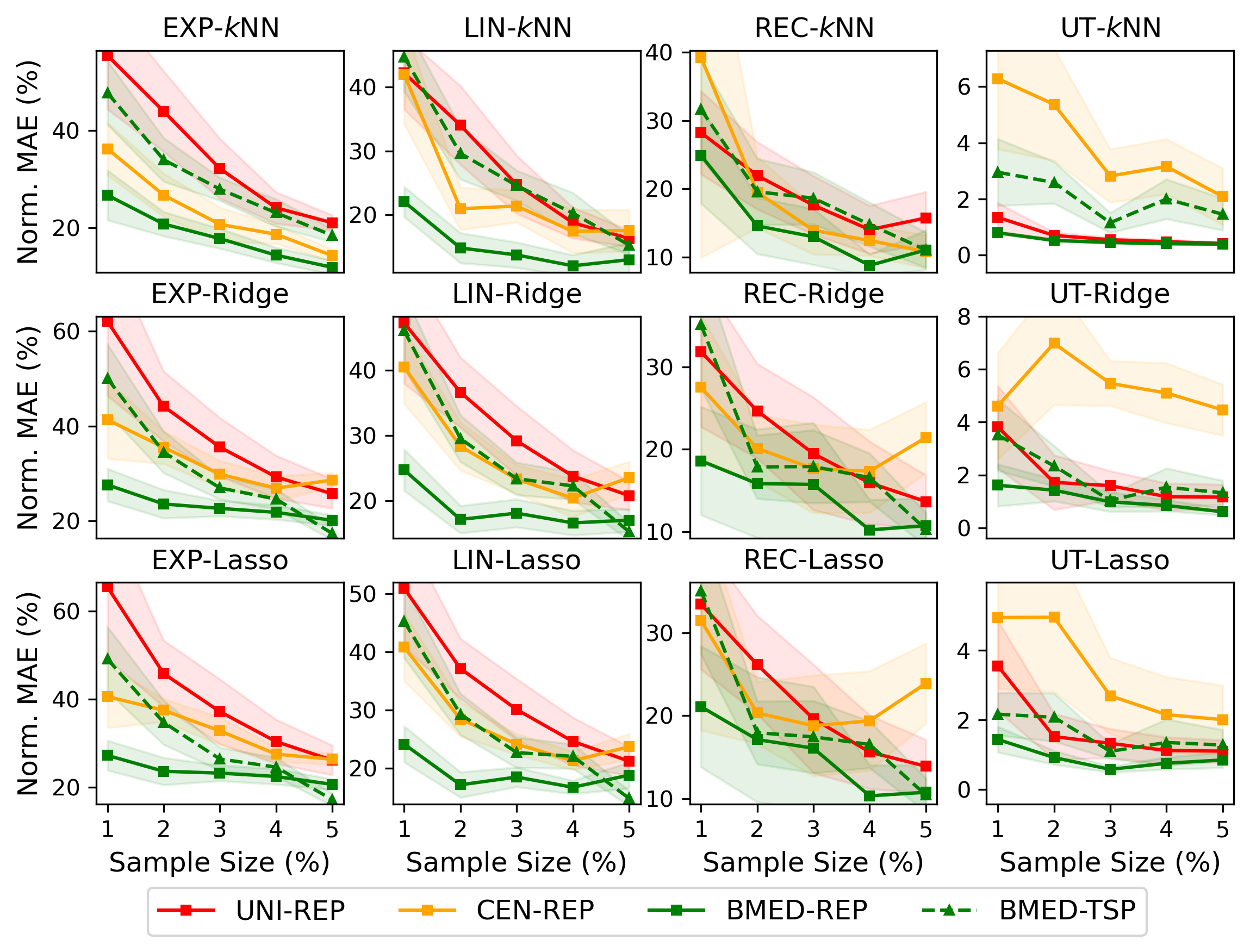
Figure 1: Mean normalized MAE ($\pm$ 95% confidence interval) over 3,000 network designs for each accessibility measure using $k$NN, lasso, and ridge regressions. Sampling methods are coded by colors. Features are coded by line types and markers. For readability, we only present the best sampling method for TSP. Details are in LABEL:subapp:add_exp1

Predictive power of the learned features. We observe that ML models generally perform better with the REP features than with the TSP features. As presented in Figure 1, when using $k$NN, the REP features outperform the TSP features by a large margin (e.g. over 44.0%, 50.7%, 21.1%, and 73.0% for EXP, LIN, REC, and UT, respectively, when the sample size is 1%). The performance gap between REP and TSP features is larger when using the $k$NN model because, as illustrated in Secition 5, the REP features are constructed to pull together followers with “similar” costs in the feature space, which favors the $k$NN model. When using lasso and ridge regression, the REP features still outperform the TSP features, highlighting the robustness of our representation learning approach. For example, when the sample size is 1%, the normalized MAE of the REP features is 33.5–47.0% lower than that of the TSP features. For additional robustness, we tested combining REP and TSP features, but found that REP alone performed the best. In other applications, combining REP features with domain-specific features could improve performance.

6.3 Experiment 2: Generating Leader Decisions using ML-augmented Models

Next, we investigate the extent to which our learned features and our follower samples can assist the ML-augmented model in generating high-quality leader (i.e., transportation planner) decisions. We consider the reduced model, $k$NN-augmented model, and linear regression-augmented model using BMED and UNI samples, totaling six methods for generating leader decisions. Results for CEN samples are in LABEL:subapp:add_exp2, as they are similar to UNI samples. We create 12 problem instances on the synthetic network (one for each pair of design budget and accessibility measure). We vary the sample size from 1% to 5%. We apply each model 10 times using 10 samples generated with different random seeds and report the average optimality gap of the leader decisions on the original problem.

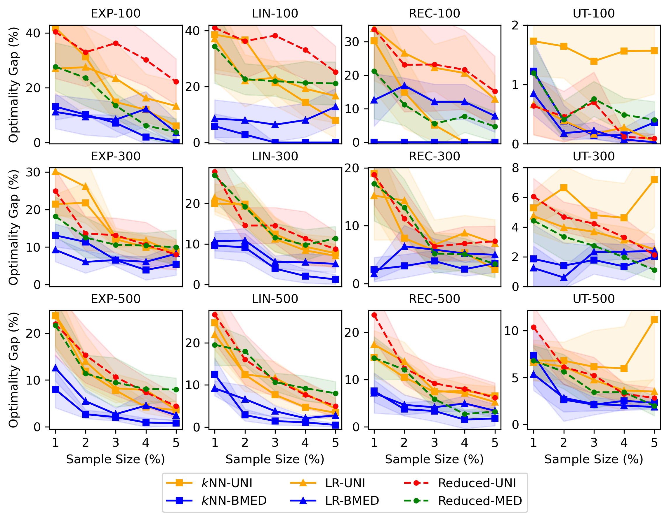
Figure 2: Mean optimality gap ($\pm$ 95% confidence interval) of leader decisions on the 12 problem instances. Problem instances follow the naming convention of “accessibility measure”-“budget” and the solution methods follow the naming convention of “model”-“sampling method”. Optimality gap $=|F(\mathbf{x}^{*})-F(\mathbf{x}^{\prime})|/F(\mathbf{x}^{*})$ where $\mathbf{x}^{*}$ and $\mathbf{x}^{\prime}$ are leader decisions from Benders decomposition and a sampling-based method, respectively.

The effectiveness of the follower selection algorithm. From Figure 2, our first observation is that using BMED samples enhances the performance of both the ML-augmented models and the reduced model. Significant performance gaps are observed for the two ML-augmented models in all problem instances. Using the BMED samples on average reduces the optimality gap by 70.5% and 54.2% for the $k$NN-augmented and linear regression-augmented models, respectively. For the reduced model, our sampling strategy is competitive with or better than uniform sampling, with an average reduction of 28.7% in optimality gap. These results highlight the importance of sample selection for both models.

The effectiveness of the ML-augmented models. Our second observation is that the best ML-augmented models ($k$NN-MED or REG-MED) generally outperform the reduced models by a large margin, especially when the sample size is extremely small (1%). This is particularly important because implementation of these models on large real-world case studies (see Section 7) are only possible when the sample size is very small ($<0.2\%$ in our case study). Moreover, the confidence intervals of the best ML-augmented model are generally narrower than those of the reduced model. The ML component helps to capture the impact of leader decisions on unsampled followers, leading to solutions of higher quality and stability. We note that the ML-augmented models may not outperform the reduced models when using the UNI samples. This is expected as the ML model is trained on an extremely small sample, necessitating careful sample selection.

Figure 3: Mean solution time ($\pm$ 95% confidence interval) on the 12 problem instances. Problem instances follow the naming convention of “accessibility measure”-“budget” and the solution methods follow the naming convention of “model”-“sampling method”.

The efficiency of the ML-augmented models. Figure 3 presents the solution time of the three models with BMED samples. In general, the solution time of all models increases as the sample size increases. The $k$NN-augmented model and the reduced model require similar solution time as the former is a re-weighted version of the latter and does not have any additional decision variables. The linear regression-augmented model generally requires longer solution time because it has more decision variables. Compared to applying Benders decomposition to the original model which generally takes over 10 hours for each instance, the ML-augmented models generate leader decisions of similar quality in 0.5–5% of the solution time, highlighting the efficiency of our method.

7 Case Study: Cycling Infrastructure Planning in the City of Toronto

In this section, we present a case study applying our methodology to the City of Toronto, Canada. Toronto has built over 65 km of new cycling infrastructure from 2019–2021, partially in response to the increased cycling demand amid the COVID-19 pandemic. It plans to expand the network by 100 km from 2022–2024. We started a collaboration with the City’s Transportation Services Team in September 2020, focusing on developing quantitative tools to support cycling infrastructure planning in Toronto. As an evaluation metric, low-stress cycling accessibility has been used by the City of Toronto to support project prioritization (City of Toronto 2021a, b). We introduce Toronto’s cycling network in Section 7.1 and use our methodology to examine actual and future potential decisions regarding network expansion in Section 7.2.

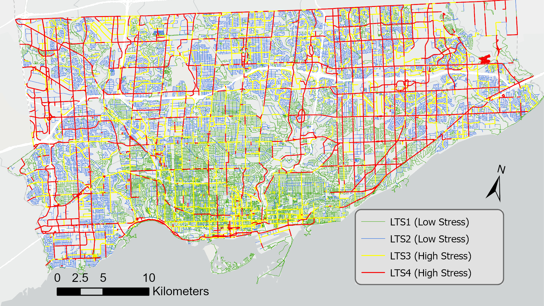
Figure 4: Level of traffic stress of Toronto’s road network (July 2021).

7.1 Cycling Network in Toronto

We construct Toronto’s cycling network based on the centerline network retrieved from the Toronto Open Data Portal (City of Toronto 2020). We pre-process the network by removing roads where cycling is legally prohibited, deleting redundant nodes and edges, and grouping arterial roads into candidate cycling infrastructure projects (detailed in LABEL:appsub:preprocessing). The final cycling network has 10,448 nodes, 35,686 edges, and 1,296 candidate projects totaling 1,913 km. We use the methods and data sources summarized in Lin et al. (2021) to calculate the LTS of each link in the cycling network. LTS1 and LTS2 links are classified as low-stress, while LTS3 and LTS4 links are high-stress since LTS2 corresponds to the cycling stress tolerance for the majority of the adult population (Furth et al. 2016). Although most local roads are low-stress, high-stress arterials create many disconnected low-stress “islands”, limiting low-stress cycling accessibility in many parts of Toronto (Figure 4).

We use the following procedure to calculate the low-stress cycling accessibility of Toronto, which serves as an evaluation metric of Toronto’s cycling network and the objective of our cycling network design problem (19). The city is divided into 3,702 geographical units called dissemination areas (DAs). We define each DA centroid as an origin with every other DA centroid that is reachable within 30 minutes on the overall network being a potential destination, totaling 1,154,663 OD pairs ($\mathcal{S}$). These OD pairs are weighted by the job counts at the destination ($q^{od}$), retrieved from the 2016 Canadian census (Statistics Canada 2016b). We use a rectangular impedance function with a cut-off time of 30 minutes ($g$). We assume a constant cycling speed of 15 km/h for travel time calculation. The resulting accessibility measure can be interpreted as the total number of jobs (services) that one can access within 30 minutes via low-stress routes in the City of Toronto. This metric has been shown to be highly correlated with cycling mode choice in Toronto (Imani et al. 2019).

7.2 Expanding Toronto’s Cycling Network

As a part of our collaboration, in January 2021 we were asked to evaluate the accessibility impact of three project alternatives for building bike lanes (see Figure 5) to meet the direction of Toronto’s City Council within the City’s adopted Cycling Network Plan, intended to provide a cycling connection between midtown and the downtown core (City of Toronto 2021b). These projects were proposed in 2019 but their evaluation and implementation were accelerated because of increased cycling demand during COVID. We determined that alternative 2 had the largest accessibility impact. It was ultimately implemented due to its accessibility impact and other performance indicators (City of Toronto 2021b).

This decision-making process exemplifies the current practice of cycling infrastructure planning in Toronto: i) manually compile a list of candidate projects, ii) rank the candidate projects based on certain metrics, and iii) design project delivery plans (City of Toronto 2021c). From a computational perspective, steps i) and ii) serve as a heuristic for solving MaxANDP. This heuristic approach was necessary for several reasons, including political buy-in for the three alternatives, and the computational intractability of solving MaxANDP at the city scale. In fact, Benders decomposition, which was used to solve the synthetic instances in Section 6, cannot find a feasible solution to these instances before running out of memory. Now, we can use our ML-augmented model to search for project combinations without pre-specifying candidates.

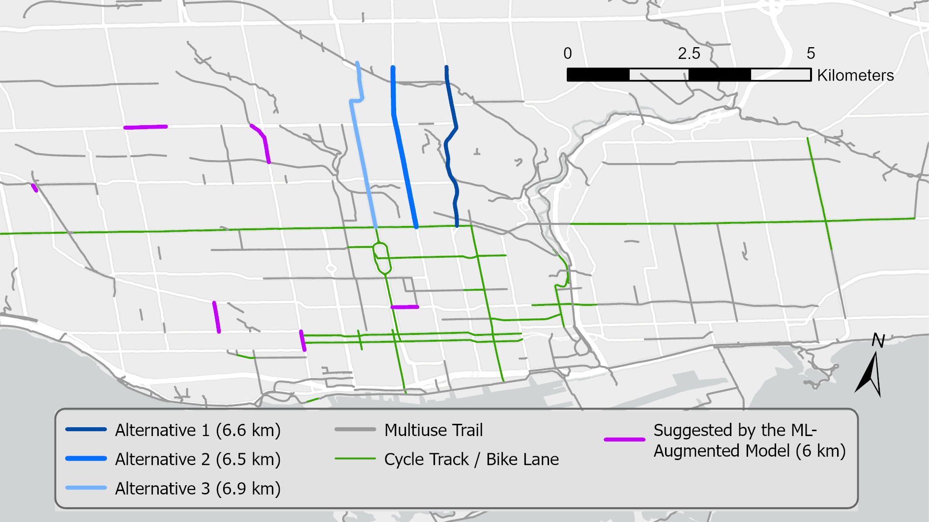
Figure 5: Project alternatives and the existing cycling infrastructure in the City of Toronto (January 2021).

To this end, we first apply the ML-augmented model with a budget of 6 km (similar to alternative 2). The optimal projects (see Figure 5) improve Toronto’s total low-stress cycling accessibility by approximately 9.5% over alternative 2. Instead of constructing only one corridor as in alternative 2, the ML-augmented model selects six disconnected road segments. Some of them serve as connections between existing cycling infrastructure, others bridge currently disconnected low-stress sub-networks consisting of low-stress local roads. We also compare our approach against i) three reduced models and ii) a greedy heuristic that iteratively selects the candidate project that leads to the maximum increase in total accessibility until the budget is depleted. As presented in Table 1, the greedy heuristic, which is commonly adopted in practice and in the existing literature, closely matches the performance of the human-proposed solution. The three reduced models are both inferior to our model, lagging behind by 5.8–34.3%. Interestingly, the greedy heuristic performs quite well against the reduced model. We believe this highlights the difficulty of achieving strong performance with a small sample in a purely sampling based model (no ML).

Table 1: Accessibility increases achieved by different solution approaches using a budget of 6 km. We implement each sampling-based method with five random samples and report the best result across the five samples.

Method (Sample)	Accessibility Increase (thousands jobs)
Human	25,553
Greedy	25,958
Reduced (UNI)	18,380
Reduced (PCEN)	21,214
Reduced (BMED)	26,350
ML-augmented (BMED)	27,968

Next, we increase the road design budget from 10 to 100 km in increments of 10 km. The 100 km budget aligns with Toronto’s cycling network expansion plan for 2022–2024 (City of Toronto 2021a). We compare our model versus the greedy heuristic to demonstrate the potential impact of our method on cycling infrastructure planning in Toronto. The greedy heuristic took over 3 days to expand the network by 100 km as each iteration involves solving millions of shortest path problems. Our approach took around 4 hours to find a leader decision using a sample of 2,000 OD pairs (1.7% of all OD pairs). Given this speedup, we can solve our model multiple times with different samples and report the best solution as measured by the total accessibility of all OD pairs. The computational setups of the greedy heuristic and our approach are detailed in LABEL:appsub:trt_comp.

As shown in Figure 6, when holding both methods to the same computational time (meaning that we solve our ML-augmented model with 21 different sets of OD pair samples and taking the best solution), our approach increases accessibility by 19.2% on average across different budgets. For example, with a budget of 70 km, we can improve the total accessibility by a similar margin as achieved by the greedy heuristic using a 100 km budget, corresponding to a savings of 18 million Canadian dollars estimated based on the City’s proposed budget (City of Toronto 2021a). If instead we used the full 100 km budget, we would achieve 11.3% greater accessibility. The improvements mainly come from identifying projects that have little accessibility impact when constructed alone, yet significantly improve the accessibility of their surrounding DAs when combined (visualized in LABEL:appsub:greedy_opt_comp). These projects are typically not directly connected to existing cycling infrastructure, and thus are difficult to identify through manual analysis. Finally, we note that solution quality was similar between 14 and 21 samples, meaning that with we can achieve the above gains while simultaneously reducing solution time by approximately 33%.

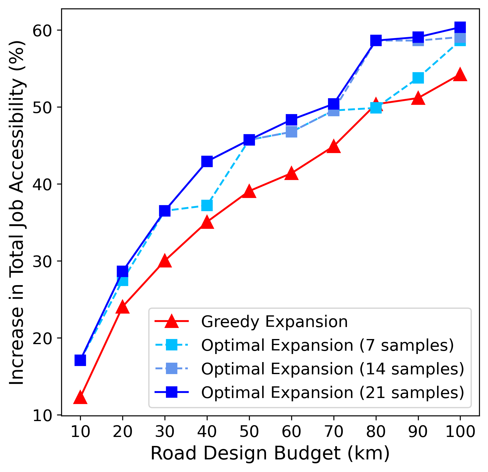
Figure 6: The performance profiles of the greedy and optimal expansions. Note that using 21 different sets of OD pairs samples results in the same solution time as the greedy expansion. Hence, 7 and 14 samples correspond to $1/3$ and $2/3$ of the solution time of greedy.

In summary, our approach is a valuable tool for transportation planners to search for optimal project combinations that maximize the low-stress cycling accessibility. Although this is not the only goal of cycling network design, we believe it can be useful in at least three contexts: i) in the long term, our model can be used to generate a base plan that can later be tuned by transportation planners; ii) in the near term, our approach can efficiently search for project combinations from a large pool that would be very difficult to analyze manually; iii) Given a fixed budget, our model provides a strong benchmark against which to validate the goodness of human-proposed solutions.

8 Conclusion

In this paper, we present a novel ML-based approach to solving bilevel (stochastic) programs with a large number of independent followers (scenarios). We build on two existing strategies—sampling and approximation—to tackle the computational challenges imposed by a large follower set. The model considers a sampled subset of followers while integrating an ML model to estimate the impact of leader decisions on unsampled followers. Unlike existing approaches for integrating optimization and ML models, we embed the ML model training into the optimization model, which allows us to employ general follower features that may not be compactly represented by leader decisions. Under certain assumptions, the generated leader decisions enjoy solution quality guarantees as measured by the original objective function considering the full follower set. We also introduce practical strategies, including follower sampling algorithms and a representation learning framework, to enhance the model performance. Using both synthetic and real-world instances of a cycling network design problem, we demonstrate the strong computational performance of our approach in generating high-quality leader decisions. The performance gap between our approach and baseline approaches are particularly large when the sample size is small.

There are several directions for future research. For example, the ML-augmented model can benefit from more advanced representation learning algorithms. The end-to-end pipeline from representation learning to the ML-augmented model can be thought of as a transfer learning framework, where we first learn general-purpose follower embedding and then fine-tune a simple ML model according to the leader decisions. Since representation learning is done before solving the optimization problem, models of any complexity might be considered. Second, the idea of embedding the training loss as a constraint has a lot of room for exploration. For example, future work can explore different loss functions or better approaches to choosing $\bar{L}$ in the parametric regression-augmented model.

The authors are grateful to Sheng Liu, Merve Bodur, Elias Khalil, Rafid Mahmood, and Erick Delage for helpful comments and discussions. This research is supported by funding from the City of Toronto and NSERC Alliance Grant 561212-20. Resources used in preparing this research were provided, in part, by the Province of Ontario, the Government of Canada through CIFAR, and companies sponsoring the Vector Institute.

Electronic Companion

9 Proofs of Solution Quality Bounds

This section presents the proof of solution quality bounds, what were omitted in the main body of this paper. This includes the proof of Theorems 4.1 and 4.2.

9.1 Proof of Theorem 4.1

Proof 9.1

Proof. Let $P$ be a non-parametric regression model as defined in equation (10), $\mathcal{T}\subseteq\mathcal{S}$ be a set of follower samples, and $\mathbf{x}_{\mathcal{T}}^{NR}$ be the leader decisions obtained by solving Problem (11). Unless otherwise noted, we write $\hat{F}_{\mathcal{T}}(\mathbf{x}_{\mathcal{T}}^{NR},P)$ as $\hat{F}_{\mathcal{T}}(\mathbf{x}_{\mathcal{T}}^{NR})$ and $w(\mathbf{f}^{s},\mathbf{f}^{t})$ as $w^{st}$ for brevity. We first decompose the optimality gap of $\mathbf{x}_{\mathcal{T}}^{NR}$ as evaluated on the bilevel model (2):

$$F(\mathbf{x}_{\mathcal{T}}^{NR})-F(\mathbf{x}^{*})$$

$$= \left[F(\mathbf{x}_{\mathcal{T}}^{NR})-\hat{F}_{\mathcal{T}}(\mathbf{x}_{\mathcal{T}}^{NR})-F(\mathbf{x}^{*})+\hat{F}_{\mathcal{T}}(\mathbf{x}^{*})\right]+\left[\hat{F}_{\mathcal{T}}(\mathbf{x}_{\mathcal{T}}^{NR})-\hat{F}_{\mathcal{T}}(\mathbf{x}^{*})\right]$$

$$\leq F(\mathbf{x}_{\mathcal{T}}^{NR})-\hat{F}_{\mathcal{T}}(\mathbf{x}_{\mathcal{T}}^{NR})-F(\mathbf{x}^{*})+\hat{F}_{\mathcal{T}}(\mathbf{x}^{*})$$

$$= \underbrace{\sum_{s\in\mathcal{S}\backslash\mathcal{T}}q^{s}\mathbb{E}[G^{s}(\mathbf{x}_{\mathcal{T}}^{NR})]-\sum_{s\in\mathcal{S}\backslash\mathcal{T}}\sum_{t\in\mathcal{T}}q^{s}w^{st}\mathbb{E}[G^{t}(\mathbf{x}_{\mathcal{T}}^{NR})]-\sum_{s\in\mathcal{S}\backslash\mathcal{T}}q^{s}\mathbb{E}[G^{s}(\mathbf{x}^{*})]+\sum_{s\in\mathcal{S}\backslash\mathcal{T}}\sum_{t\in\mathcal{T}}q^{s}w^{st}\mathbb{E}[G^{t}(\mathbf{x}^{*})]}_{\textrm{(1)}}$$

$$\underbrace{+\sum_{s\in\mathcal{S}\backslash\mathcal{T}}q^{s}G^{s}(\mathbf{x}_{\mathcal{T}}^{NR})-\sum_{s\in\mathcal{S}\backslash\mathcal{T}}\sum_{t\in\mathcal{T}}q^{s}w^{st}G^{t}(\mathbf{x}_{\mathcal{T}}^{NR})-\sum_{s\in\mathcal{S}\backslash\mathcal{T}}q^{s}\mathbb{E}[G^{s}(\mathbf{x}_{\mathcal{T}}^{NR})]+\sum_{s\in\mathcal{S}\backslash\mathcal{T}}\sum_{t\in\mathcal{T}}q^{s}w^{st}\mathbb{E}[G^{t}(\mathbf{x}_{\mathcal{T}}^{NR})]}_{\textrm{(2)}}$$

$$\underbrace{-\sum_{s\in\mathcal{S}\backslash\mathcal{T}}q^{s}G^{s}(\mathbf{x}^{*})+\sum_{s\in\mathcal{S}\backslash\mathcal{T}}\sum_{t\in\mathcal{T}}q^{s}w^{st}G^{t}(\mathbf{x}^{*})+\sum_{s\in\mathcal{S}\backslash\mathcal{T}}q^{s}\mathbb{E}[G^{s}(\mathbf{x}^{*})]-\sum_{s\in\mathcal{S}\backslash\mathcal{T}}\sum_{t\in\mathcal{T}}q^{s}w^{st}\mathbb{E}[G^{t}(\mathbf{x}^{*})]}_{\textrm{(3)}}$$

The third line holds because $\mathbf{x}_{\mathcal{T}}^{NR}$ is the optimal solution to problem (11). We derive the final equation by i) writing the extensive form of functions $F$ and $\hat{F}_{\mathcal{T}}$, and ii) adding and subtracting the expected values of them. Next, we bound (1) and (2) + (3), separately, which will eventually be combined to derive a bound on (1) + (2) + (3).

According to the Lipschitz property described by Assumption 4.2.2, we have

$$(1)\leq \sum_{s\in\mathcal{S}\backslash\mathcal{T}}\sum_{t\in\mathcal{T}}q^{s}w^{st}\left\{\left|\mathbb{E}[G^{s}(\mathbf{x}_{\mathcal{T}}^{NR})]-\mathbb{E}[G^{t}(\mathbf{x}_{\mathcal{T}}^{NR})]\right|+\left|\mathbb{E}[G^{s}(\mathbf{x}^{*})]-\mathbb{E}[G^{t}(\mathbf{x}^{*})]\right|\right\}$$

$$\leq \sum_{s\in\mathcal{S}\backslash\mathcal{T}}\sum_{t\in\mathcal{T}}2\mu\bar{Q}w^{st}d_{\mathcal{F}}(\mathbf{f}^{s},\mathbf{f}^{t}).$$

Let $w^{t}=\sum_{s\in\mathcal{S}\backslash\mathcal{T}}w^{st}$ for all $t\in\mathcal{T}$. We have

$$(2)+(3)=\bar{Q}\left[\sum_{s\in\mathcal{S}\backslash\mathcal{T}}\left[G^{s}(\mathbf{x}_{\mathcal{T}}^{NR})-G^{s}(\mathbf{x}^{*})\right]-\sum_{t\in\mathcal{T}}w^{t}\left[G^{t}(\mathbf{x}_{\mathcal{T}}^{NR})-G^{t}(\mathbf{x}^{*})\right]\right.\\ \left.-\sum_{s\in\mathcal{S}\backslash\mathcal{T}}\mathbb{E}[G^{s}(\mathbf{x}_{\mathcal{T}}^{NR})-G^{s}(\mathbf{x}^{*})]+\sum_{t\in\mathcal{T}}w^{t}\mathbb{E}[G^{t}(\mathbf{x}_{\mathcal{T}}^{NR})-G^{t}(\mathbf{x}^{*})]\right].$$

According to Assumptions 4.2.2 and 4.2.2, we can regard $\left[G^{s}(\mathbf{x}_{\mathcal{T}}^{NR})-G^{s}(\mathbf{x}^{*})\right]$ as independent random variables that are bounded in an interval of length $2\bar{G}$ almost surely. Similarly, independent random variables $w^{t}\left[G^{t}(\mathbf{x}_{\mathcal{T}}^{NR})-G^{t}(\mathbf{x}^{*})\right]$ are bounded in an interval of length $2w^{t}\bar{G}$ almost surely. By applying Hoeffding inequality (Hoeffding 1994), we have, with probability at least $1-\gamma$,

$$(2)+(3)\leq \sqrt{2\bar{Q}^{2}\bar{G}^{2}\left[|\mathcal{S}\backslash\mathcal{T}|+\sum_{t\in\mathcal{T}}(w^{t})^{2}\right]\log(1/\gamma)}.$$

We therefore conclude that with probability at least $1-\gamma$,

$$F(\mathbf{x}_{\mathcal{T}}^{NR})-F(\mathbf{x}^{*})\leq\sum_{s\in\mathcal{S}\backslash\mathcal{T}}\sum_{t\in\mathcal{T}_{k}(\mathbf{f}^{s})}2\mu\bar{Q}w^{st}d_{\mathcal{F}}(\mathbf{f}^{s},\mathbf{f}^{t})+\sqrt{2\bar{Q}^{2}\bar{G}^{2}\left[|\mathcal{S}\backslash\mathcal{T}|+\sum_{t\in\mathcal{T}}(w^{t})^{2}\right]\log(1/\gamma)}.$$

9.2 Proof of Theorem 4.2

Proof 9.2

Proof. Let $P$ be parametric regression model, $\mathcal{T}\subseteq\mathcal{S}$ be a set of follower samples, and ($\mathbf{x}_{\mathcal{T}}^{NR}$, $\boldsymbol{\theta}_{\mathcal{T}}$) be the optimal solution to Problem (12), ($\mathbf{x}^{*}$, $\boldsymbol{\theta}^{*}$) be an feasible solution to Problem (12). Unless otherwise noted, we write $\hat{F}_{\mathcal{T}}(\mathbf{x}_{\mathcal{T}}^{PR},P)$ as $\hat{F}_{\mathcal{T}}$. We first decompose the optimality gap of $\mathbf{x}_{\mathcal{T}}^{PR}$ as evaluated on the bilevel model (2):

$$F(\mathbf{x}_{\mathcal{T}}^{PR})-F(\mathbf{x}^{*})$$

$$= \left[F(\mathbf{x}_{\mathcal{T}}^{PR})-\hat{F}_{\mathcal{T}}(\mathbf{x}_{\mathcal{T}}^{PR},\boldsymbol{\theta}_{\mathcal{T}})-F(\mathbf{x}^{*})+\hat{F}_{\mathcal{T}}(\mathbf{x}^{*},\boldsymbol{\theta}^{*})\right]+\left[\hat{F}_{\mathcal{T}}(\mathbf{x}_{\mathcal{T}}^{PR},\boldsymbol{\theta}_{\mathcal{T}})-\hat{F}_{\mathcal{T}}(\mathbf{x}^{*},\boldsymbol{\theta}^{*})\right]$$

$$\leq F(\mathbf{x}_{\mathcal{T}}^{PR})-\hat{F}_{\mathcal{T}}(\mathbf{x}_{\mathcal{T}}^{PR},\boldsymbol{\theta}_{\mathcal{T}})-F(\mathbf{x}^{*})+\hat{F}_{\mathcal{T}}(\mathbf{x}^{*},\boldsymbol{\theta}^{*})$$

$$\leq \underbrace{\sum_{s\in\mathcal{S}\backslash\mathcal{T}}q^{s}\mathbb{E}[G^{s}(\mathbf{x}_{\mathcal{T}}^{PR})]-\sum_{s\in\mathcal{S}\backslash\mathcal{T}}q^{s}\mathbb{E}[G^{\nu(s)}(\mathbf{x}_{\mathcal{T}}^{PR})]-\sum_{s\in\mathcal{S}\backslash\mathcal{T}}q^{s}\mathbb{E}[G^{s}(\mathbf{x}^{*})]+\sum_{s\in\mathcal{S}\backslash\mathcal{T}}q^{s}\mathbb{E}[G^{\nu(s)}(\mathbf{x}^{*})]}_{\textrm{(1)}}$$

$$\underbrace{+\sum_{s\in\mathcal{S}\backslash\mathcal{T}}q^{s}P(\mathbf{f}^{\nu(s)};\boldsymbol{\theta}_{\mathcal{T}})-\sum_{s\in\mathcal{S}\backslash\mathcal{T}}q^{s}P(\mathbf{f}^{s};\boldsymbol{\theta}_{\mathcal{T}})-\sum_{s\in\mathcal{S}\backslash\mathcal{T}}q^{s}P(\mathbf{f}^{\nu(s)};\boldsymbol{\theta}^{*})+\sum_{s\in\mathcal{S}\backslash\mathcal{T}}q^{s}P(\mathbf{f}^{s};\boldsymbol{\theta}^{*})}_{\textrm{(2)}}$$

$$\underbrace{+\sum_{s\in\mathcal{S}\backslash\mathcal{T}}q^{s}G^{\nu(s)}(\mathbf{x}_{\mathcal{T}}^{PR})-\sum_{s\in\mathcal{S}\backslash\mathcal{T}}q^{s}P(\mathbf{f}^{\nu(s)};\boldsymbol{\theta}_{\mathcal{T}})-\sum_{s\in\mathcal{S}\backslash\mathcal{T}}q^{s}G^{\nu(s)}(\mathbf{x}^{*})+\sum_{s\in\mathcal{S}\backslash\mathcal{T}}q^{s}P(\mathbf{f}^{\nu(s)};\boldsymbol{\theta}^{*})}_{\textrm{(3)}}$$

$$\underbrace{+\sum_{s\in\mathcal{S}\backslash\mathcal{T}}q^{s}G^{s}(\mathbf{x}_{\mathcal{T}}^{PR})-\sum_{s\in\mathcal{S}\backslash\mathcal{T}}q^{s}\mathbb{E}[G^{s}(\mathbf{x}_{\mathcal{T}}^{PR})]+\sum_{s\in\mathcal{S}\backslash\mathcal{T}}q^{s}\mathbb{E}[G^{\nu(s)}(\mathbf{x}_{\mathcal{T}}^{PR})]-\sum_{s\in\mathcal{S}\backslash\mathcal{T}}q^{s}G^{\nu(s)}(\mathbf{x}_{\mathcal{T}}^{PR})}_{\textrm{(4)}}$$

$$\underbrace{-\sum_{s\in\mathcal{S}\backslash\mathcal{T}}q^{s}G^{s}(\mathbf{x}^{*})+\sum_{s\in\mathcal{S}\backslash\mathcal{T}}q^{s}\mathbb{E}[G^{s}(\mathbf{x}^{*})]-\sum_{s\in\mathcal{S}\backslash\mathcal{T}}q^{s}\mathbb{E}[G^{\nu(s)}(\mathbf{x}^{*})]+\sum_{s\in\mathcal{S}\backslash\mathcal{T}}q^{s}G^{\nu(s)}(\mathbf{x}^{*})}_{\textrm{(5)}}$$

According to Assumption 4.2.2, we have

$$(1)\leq\sum_{s\in\mathcal{S}\backslash\mathcal{T}}q^{s}\left\{\left|\mathbb{E}[G^{s}(\mathbf{x}^{PR}_{\mathcal{T}})]-\mathbb{E}[G^{\nu(s)}(\mathbf{x}^{PR}_{\mathcal{T}})]\right|+\left|\mathbb{E}[G^{s}(\mathbf{x}^{*})]-\mathbb{E}[G^{\nu(s)}(\mathbf{x}^{*})]\right|\right\}\leq 2\mu\bar{Q}\sum_{s\in\mathcal{S}\backslash\mathcal{T}}d_{\mathcal{F}}(\mathbf{f}^{s},\mathbf{f}^{\nu(s)})$$

According to the Lipschitz Property of $P$, we have

$$(2)\leq\sum_{s\in\mathcal{S}\backslash\mathcal{T}}q^{s}\left\{\left|P(\mathbf{f}^{\nu(s)};\boldsymbol{\theta}_{\mathcal{T}})-P(\mathbf{f}^{s};\boldsymbol{\theta}_{\mathcal{T}})\right|+\left|P(\mathbf{f}^{\nu(s)};\boldsymbol{\theta}^{*})-P(\mathbf{f}^{s};\boldsymbol{\theta}^{*})\right|\right\}\leq 2\lambda\bar{Q}\sum_{s\in\mathcal{S}\backslash\mathcal{T}}d_{\mathcal{F}}(\mathbf{f}^{s},\mathbf{f}^{\nu(s)})$$

Since the training loss of $P$ is bounded by $\bar{L}$, we have

$$(3)\leq\bar{Q}\left\{\sum_{t\in\mathcal{T}}m^{t}_{1,\mathcal{S}\backslash\mathcal{T}}\left|P(\mathbf{f}^{t};\boldsymbol{\theta}_{\mathcal{T}})-G^{t}(\mathbf{x}^{PR}_{\mathcal{T}})\right|+\sum_{t\in\mathcal{T}}m^{t}_{1,\mathcal{S}\backslash\mathcal{T}}\left|P(\mathbf{f}^{t};\boldsymbol{\theta}^{*})-G^{t}(\mathbf{x}^{*})\right|\right\}\leq 2\bar{Q}\bar{L}$$

We have

$$(4)+(5)=\bar{Q}\left\{\sum_{s\in\mathcal{S}}\left[G^{s}(\mathbf{x}^{PR}_{\mathcal{T}})-G^{s}(\mathbf{x}^{*})\right]-\sum_{t\in\mathcal{T}}m^{t}_{1,\mathcal{S}\backslash\mathcal{T}}\left[G^{t}(\mathbf{x}^{PR}_{\mathcal{T}})-G^{t}(\mathbf{x}^{*})\right]\right.\\ \left.-\sum_{s\in\mathcal{S}}\mathbb{E}\left[G^{s}(\mathbf{x}^{PR}_{\mathcal{T}})-G^{s}(\mathbf{x}^{*})\right]+\sum_{t\in\mathcal{T}}m^{t}_{1,\mathcal{S}\backslash\mathcal{T}}\mathbb{E}\left[G^{t}(\mathbf{x}^{PR}_{\mathcal{T}})-G^{t}(\mathbf{x}^{*})\right]\right\}$$

According to the Assumptions 4.2.2 and 4.2.2, we can regard $\left[G^{s}(\mathbf{x}^{PR}_{\mathcal{T}})-G(\mathbf{x}^{*})\right]$ as independent random variables that are bounded in an interval of length $2\bar{G}$ almost surely. Similarly, independent random variables $-m^{t}_{1,\mathcal{S}\backslash\mathcal{T}}\left[G^{t}(\mathbf{x}^{PR}_{\mathcal{T}})-G^{t}(\mathbf{x}^{*})\right]$ are bounded in an interval of length $2m^{t}_{1,\mathcal{S}\backslash\mathcal{T}}\bar{G}$ almost surely. By applying Hoeffding inequality (Hoeffding 1994), we have, with probability at least $1-\gamma$,

$$(4)+(5)\leq\sqrt{2\bar{Q}^{2}\bar{G}^{2}\left[|\mathcal{S}\backslash\mathcal{T}|+\sum_{t\in\mathcal{T}}(m^{t}_{1,\mathcal{S}\backslash\mathcal{T}})^{2}\right]\log(1/\gamma)}$$

We therefore conclude that with probability at least $1-\gamma$,

$$F(\mathbf{x}^{PR}_{\mathcal{T}})-F(\mathbf{x}^{*})\leq 2\bar{Q}\bar{L}+2\bar{Q}(\lambda+\mu)\sum_{s\in\mathcal{S}\backslash\mathcal{T}}d_{\mathcal{F}}(\mathbf{f}^{s},\mathbf{f}^{\nu(s)})+\sqrt{2\bar{Q}^{2}\bar{G}^{2}\left[|\mathcal{S}\backslash\mathcal{T}|+\sum_{t\in\mathcal{T}}(m^{t}_{1,\mathcal{S}\backslash\mathcal{T}})^{2}\right]\log(1/\gamma)}$$

10 Proofs of Bound Tightness Results

This section presents the proof of our bound tightness results that were omitted in the main body of this paper, including Proposition 4.4 and Theorems 4.5 and 4.6.

10.1 Proof of Proposition 4.4

Proof 10.1

Proof. Based on the definition of $\mathcal{T}_{k}$, we have for any $s\in\backslash\mathcal{T}$ and $k\in[1,p-1]$,

$$\mathcal{T}_{k}(\mathbf{f}^{s})\subset\mathcal{T}_{k+1}(\mathbf{f}^{s}).$$

Therefore,

$$M(k,\mathcal{T}) =\sum_{s\in\mathcal{S}\backslash\mathcal{T}}\sum_{t\in\mathcal{T}_{k}(\mathbf{f}^{s})}d_{\mathcal{F}}(\mathbf{f}^{s},\mathbf{f}^{t}).\leq\sum_{s\in\mathcal{S}\backslash\mathcal{T}}\sum_{t\in\mathcal{T}_{k+1}(\mathbf{f}^{s})}d_{\mathcal{F}}(\mathbf{f}^{s},\mathbf{f}^{t})=M(k+1,\mathcal{T}).$$

10.2 Proof of Theorem 4.5

We start by proving two useful lemmas that will later be brought together to prove Theorem 4.5. For convenience, we re-state the definition of $E^{NR}$ when using the $1$-NN weighting scheme.

$$E^{NR}_{m}(\mathcal{T})=2\mu\bar{Q}M(1,\mathcal{T})+\sqrt{2\bar{Q}^{2}\bar{G}^{2}\left[m-p+\sum_{t\in\mathcal{T}}(m^{t}_{1,\mathcal{S}\backslash\mathcal{T}})^{2}\right]\log(1/\gamma)}.$$

Lemma 10.2

For any $\mathcal{T}\subset\mathcal{S}$ that is feasible to problem (13) and $(\mathbf{f}^{1},\mathbf{f}^{2},\dots,\mathbf{f}^{m})$ for some $m\in\mathbb{N}_{+}$, we have $0\leq E^{NR}_{m}(\mathcal{T})\leq\bar{E}_{m}^{NR}(\mathcal{T})$ where

$$\bar{E}^{NR}_{m}(\mathcal{T})=2\mu\bar{Q}M(1,\mathcal{T})+\sqrt{2\bar{Q}^{2}\bar{G}^{2}\left[m-p+pd^{2}\right]\log(1/\gamma)}$$

Proof 10.3

Proof. The first inequality is trivial. The second inequality holds because $|\mathcal{S}\backslash\mathcal{T}|=m-p$ and $m_{1,\backslash\mathcal{T}}^{t}=|\mathcal{S}(t)|\leq d$ for all $t\in\mathcal{T}$ which come from the constraints in problem (13).

Lemma 10.4

If $(\mathbf{f}^{1},\mathbf{f}^{2},\dots,\mathbf{f}^{m})$ is a sequence of i.i.d. random points in $[0,1]^{\xi}$ with a continuous density $\sigma(\mathbf{f})$, $p=\max\{1,\alpha m\}$ for some $\alpha\in(0,1]$, and $\lceil m/p\rceil\leq d\leq\beta\lceil m/p\rceil$ for some $\beta\geq 1$, then we have

$$\lim_{m\rightarrow\infty}\frac{1}{m}\bar{E}^{NR}_{m}(\mathcal{T}_{p,d})=0.$$

Proof 10.5

Proof. We first derive the limit of the second term in $\bar{E}_{m}^{NR}$. We have

$$0\leq\frac{1}{m}\sqrt{2\bar{Q}^{2}\bar{G}^{2}\left[m-p+pd^{2}\right]\log(1/\gamma)}\leq\sqrt{2\bar{Q}^{2}\bar{G}^{2}\left[\frac{1}{m}-\frac{\alpha}{m}+\frac{\beta^{2}}{\alpha m^{(\xi-1)/\xi}}\right]\log(1/\gamma)}.$$

By the Squeeze theorem, we have

$$\lim_{m\rightarrow\infty}\frac{1}{m}\sqrt{2\bar{Q}^{2}\bar{G}^{2}\left[m-p+pd^{2}\right]\log(1/\gamma)}=0.$$ (22)

We next derive the limit of the first term in $\bar{E}_{m}^{NR}$. According to Theorem 1.1 from McGivney and Yukich (1999), we have

$$\lim_{m\rightarrow\infty}\frac{1}{m^{(\xi-1)/\xi}}M(1,\mathcal{T})=C_{d,\xi}\int_{[0,1]^{\xi}}\sigma^{(\xi-1)/\xi}(\mathbf{f})df.$$ (23)

where $C_{d,\xi}>0$ is a constant that depends on $d$ and $\xi$. As estimated in Theorem 12 from Carlsson and Jones (2022), $C_{d,\xi}$ satisfies

$$C_{d,\xi}\leq\frac{2}{3}\sqrt{d}.$$ (24)

Given equations (23) and (24) and that $d\leq\beta\lceil m/p\rceil$ and $p=\max\{1,\alpha m^{(\xi-1)/\xi}\}$,

$$\lim_{m\rightarrow\infty}\frac{1}{m}M(1,\mathcal{T})=0.$$ (25)

Combining equations (22) and (25), we have

$$\lim_{m\rightarrow\infty}\frac{1}{m}\bar{E}^{NR}_{m}(\mathcal{T}_{p,d})=0.$$

Proof 10.6

Proof of Theorem 4.5. By Lemmas 10.2 and 10.4 and the Squeeze Theorem, we have

$$\lim_{m\rightarrow\infty}\frac{1}{m}E^{NR}_{m}(\mathcal{T}_{p,d})=0.$$

10.3 Proof of Theorem 4.6

We first prove two lemmas that are useful for proving Theorem 4.6. For convenience, we restate the definition of $E^{PR}_{m}$:

$$E^{PR}_{m}(\mathcal{T},\bar{L})=2\bar{Q}\bar{L}+2\bar{Q}(\lambda+\mu)M(1,\mathcal{T})+\sqrt{2\bar{Q}^{2}\bar{G}^{2}\left[m-p+\sum_{t\in\mathcal{T}}(m^{t}_{1,\mathcal{S}\backslash\mathcal{T}})^{2}\right]\log(1/\gamma)}.$$

Lemma 10.7

For any $\mathcal{T}\subset\mathcal{S}$ that is feasible to problem (13), $(\mathbf{f}^{1},\mathbf{f}^{2},\dots,\mathbf{f}^{m})$ for some $m\in\mathbb{N}_{+}$, and $\bar{L}>0$, we have $0\leq E^{PR}_{m}(\mathcal{T},\bar{L})\leq\bar{E}^{PR}_{m}(\mathcal{T},\bar{L})$ where

$$\bar{E}^{PR}_{m}(\mathcal{T},\bar{L})=2\bar{Q}\bar{L}+2\bar{Q}(\lambda+\mu)M(1,\mathcal{T})+\sqrt{2\bar{Q}^{2}\bar{G}^{2}\left[m-p+pd^{2}\right]\log(1/\gamma).}$$

Proof 10.8

Proof. Similar to Lemma 10.2, the second inequality holds because of the constraints $|\mathcal{S}(t)|\leq d$ in Problem (13).

Lemma 10.9

If $(\mathbf{f}^{1},\mathbf{f}^{2},\dots,\mathbf{f}^{m})$ is a sequence of i.i.d. random points in $[0,1]^{\xi}$ with density $\sigma(\mathbf{f})$, $p=\max\{1,\alpha m\}$ for some $\alpha\in(0,1]$, $\lceil m/p\rceil\leq d\leq\beta\lceil m/p\rceil$ for some $\beta\geq 1$, and $\bar{L}$ is a finite positive constant, then

$$\lim_{m\rightarrow\infty}\frac{1}{m}\bar{E}^{PR}_{m}(\mathcal{T}_{p,d})=0.$$

Proof 10.10

Proof. Since $\bar{L}$ is a finite positive constant, according to equations (22) and (25),

$$\lim_{m\rightarrow\infty}\frac{1}{m}\bar{E}^{PR}_{m}(\mathcal{T}_{p,d},\bar{L})=0.$$

Proof 10.11

Proof of Theorem 4.6. According to Lemmas 10.7 and 10.9 and the Squeeze Theorem,

$$\lim_{m\rightarrow\infty}\frac{1}{m}E^{PR}_{m}(\mathcal{T}_{p,d},\bar{L})=0$$

11 Proofs of Representation Learning Results

11.1 Proof of Lemma 17

Proof 11.1

Proof. Let $\boldsymbol{\lambda}^{*}$ denote an optimal solution to Problem (15) and $p^{st*}=p^{st}(\boldsymbol{\lambda}^{*})$. According to equation (16), we have

$$\sum_{t\in[n]}p^{st*}=1,\quad\forall s\in[n].$$

Therefore, for any $s\in[n]$, $\mathbf{p}^{s*}:=[p^{s1*},p^{s2*},\ldots,p^{sn*}]$ is an optimal solution to the following optimization problem:

$$\underset{\mathbf{p}\in\mathbb{R}^{n}_{+}}{\textrm{maximize}}\quad \prod_{t\in[n]}\left[p^{st}\right]^{n^{st}}$$ (26a)

subject to $$\sum_{t\in[n]}p^{st}=1.$$ (26b)

where $n^{st}$ denote the number of times that node $t$ appear after node $s$ in random walks $\{\mathcal{W}\}_{i\in[n],j\in[n_{\textrm{walk}}]}$. Writing the Lagrangian relaxation for Problem (26), we obtain

$$L(\mathbf{p},\mu)=\prod_{t\in[n]}\left[p^{st}\right]^{n^{st}}+\mu(\sum_{t\in[n]}p^{st}-1)$$ (27)

where $\mu\in\mathbb{R}$ is the Lagrangian multiplier of constraint (26b). By applying the Lagrangian condition, we know that $\mathbf{p}^{s*}$ satisfy

$$p^{st*}=\frac{n^{st}}{\sum_{k\in[n]}n^{sk}}.$$ (28)

Given the random-walk generation process described in Algorithm 1, according to the law of large number, we have

$$\lim_{n_{\textrm{walk}}\rightarrow+\infty}p^{st*}=\lim_{n_{\textrm{walk}}\rightarrow+\infty}\frac{n^{st}}{\sum_{k\in[n]}n^{sk}}=\frac{\pi^{st}}{\sum_{k\in[n]}\pi^{sk}},$$ (29)

which completes the proof.

11.2 Proof of Proposition 18

Proof 11.2

Proof. According to Lemma 17, for any $(s,t)\in[n]\times[n]$, we have

$$\frac{\exp[(\mathbf{f}^{s})^{\intercal}\mathbf{f}^{t}]}{\sum_{k\in[n]}\exp[(\mathbf{f}^{s})^{\intercal}\mathbf{f}^{k}]}=\frac{\pi^{st}}{\sum_{k\in[n]}\pi^{sk}}.$$ (30)

Therefore,

$$\exp[(\mathbf{f}^{s})^{\intercal}\mathbf{f}^{t}]=\alpha\pi^{st},$$ (31)

where $\alpha=\exp\left[(\mathbf{f}^{s})^{\intercal}\mathbf{f}^{s}\right]$ because $\pi^{ss}=0$ for any $s\in[n]$. Note that this also implies that $\|\mathbf{f}^{s}\|=\|\mathbf{f}^{t}\|$ for any $(s,t)\in[n]\times[n]$.

Let $d_{\mathcal{F}}(\cdot,\cdot)$ be a function that calculates the cosine distance between two vectors in the feature space $\mathcal{F}$. For any $(s,t)\in[n]\times[n]$,

$$d_{\mathcal{F}}(\mathbf{f}^{s},\mathbf{f}^{t})=\frac{1}{2}-\frac{(\mathbf{f}^{s})^{\intercal}\mathbf{f}^{t}}{2\|\mathbf{f}^{s}\|\|\mathbf{f}^{t}\|}=\frac{1}{2}-\frac{\log\alpha+\log\pi^{st}}{2\log\alpha}\leq\frac{1}{2n_{\textrm{sim}}\log\alpha}\sum_{i=1}^{n_{\textrm{sim}}}\left|G^{i}_{s}-G^{i}_{t}\right|.$$ (32)

The last inequality holds because $\Phi$ is a sub-exponential function. Therefore, we have for any $(s,t)\in[n]\times[n]$,

$$2\log\alpha d_{\mathcal{F}}(\mathbf{f}^{s},\mathbf{f}^{t})\geq\frac{1}{n_{\textrm{sim}}}\sum_{i=1}^{n_{\textrm{sim}}}\left|G^{i}_{s}-G^{i}_{t}\right|,$$

which completes the proof.

12 ML-Augmented Model with Alternative Loss Functions

In this section, we present ML-augmented models with alternative loss functions and their associated sub-optimality bounds. Proofs are also included.

12.1 $L_{2}$ loss

When using the $L_{2}$ loss, the ML-augmented model becomes

$$\min_{\mathbf{x}\in\mathcal{X},\boldsymbol{\theta}\in\boldsymbol{\Theta}}\left\{f(\mathbf{x})+\sum_{t\in\mathcal{T}}G^{t}(\mathbf{y})+\sum_{s\in\mathcal{S}\backslash\mathcal{T}}P(\mathbf{f}^{s};\boldsymbol{\theta})\,\middle|\,\sum_{t\in\mathcal{T}}\left|G^{t}(\mathbf{y})-P(\mathbf{f}^{t};\boldsymbol{\theta})\right|^{2}\leq\bar{L}\right\}.$$ (33)

Theorem 12.1

Given a follower sample $\mathcal{T}\subseteq\mathcal{S}$, let $P$ be a parametric ML model, $\mathbf{x}^{PR}_{\mathcal{T},l_{2}}$ be the optimal solution to Problem (33), $\nu(s)$ be the nearest neighbor of $\mathbf{f}^{s}$ in $\{\mathbf{f}^{t}\}_{t\in\mathcal{T}}$, and $m^{t}_{1,\mathcal{S}\backslash\mathcal{T}}=\sum_{s\in\mathcal{S}\backslash\mathcal{T}}\mathds{1}[\nu(s)=t]$. If Assumptions 4.2.2–4.2.2 hold, with probability at least $1-\gamma$, $F(\mathbf{x}^{PR}_{\mathcal{T},l_{2}})-F(\mathbf{x}^{*})\leq E_{m,l_{2}}^{PR}(\mathcal{T},\bar{L})$ where

$$E_{m,l_{2}}^{PR}(\mathcal{T},\bar{L})=2\bar{Q}(\lambda+\mu)\sum_{s\in\mathcal{S}\backslash\mathcal{T}}d_{\mathcal{F}}(\mathbf{f}^{s},\mathbf{f}^{\nu(s)})+2\bar{Q}\sqrt{\bar{L}\sum_{t\in\mathcal{T}}(m^{t}_{1,\mathcal{S}\backslash\mathcal{T}})^{2}}\\ +\sqrt{2\bar{Q}^{2}\bar{G}^{2}\left[|\mathcal{S}\backslash\mathcal{T}|+\sum_{t\in\mathcal{T}}(m^{t}_{1,\mathcal{S}\backslash\mathcal{T}})^{2}\right]\log(1/\gamma)}.$$ (34)

Proof 12.2

Proof The proof of Theorem 12.1 largely follows the proof of Theorem 4.2. For clarity, we present the full proof below and highlight the difference between them in the end.

Let $P$ be parametric regression model, $\mathcal{T}\subseteq\mathcal{S}$ be a set of follower samples, and ($\mathbf{x}_{\mathcal{T}}^{NR}$, $\boldsymbol{\theta}_{\mathcal{T}}$) be the optimal solution to Problem (33), ($\mathbf{x}^{*}$, $\boldsymbol{\theta}^{*}$) be an feasible solution to Problem (33). Unless otherwise noted, we write $\hat{F}_{\mathcal{T}}(\mathbf{x}_{\mathcal{T}}^{PR},P)$ as $\hat{F}_{\mathcal{T}}$. We first decompose the optimality gap of $\mathbf{x}_{\mathcal{T}}^{PR}$ as evaluated on the bilevel model (2):

$$F(\mathbf{x}_{\mathcal{T}}^{PR})-F(\mathbf{x}^{*})$$

$$= \left[F(\mathbf{x}_{\mathcal{T}}^{PR})-\hat{F}_{\mathcal{T}}(\mathbf{x}_{\mathcal{T}}^{PR},\boldsymbol{\theta}_{\mathcal{T}})-F(\mathbf{x}^{*})+\hat{F}_{\mathcal{T}}(\mathbf{x}^{*},\boldsymbol{\theta}^{*})\right]+\left[\hat{F}_{\mathcal{T}}(\mathbf{x}_{\mathcal{T}}^{PR},\boldsymbol{\theta}_{\mathcal{T}})-\hat{F}_{\mathcal{T}}(\mathbf{x}^{*},\boldsymbol{\theta}^{*})\right]$$

$$\leq F(\mathbf{x}_{\mathcal{T}}^{PR})-\hat{F}_{\mathcal{T}}(\mathbf{x}_{\mathcal{T}}^{PR},\boldsymbol{\theta}_{\mathcal{T}})-F(\mathbf{x}^{*})+\hat{F}_{\mathcal{T}}(\mathbf{x}^{*},\boldsymbol{\theta}^{*})$$

$$\leq \underbrace{\sum_{s\in\mathcal{S}\backslash\mathcal{T}}q^{s}\mathbb{E}[G^{s}(\mathbf{x}_{\mathcal{T}}^{PR})]-\sum_{s\in\mathcal{S}\backslash\mathcal{T}}q^{s}\mathbb{E}[G^{\nu(s)}(\mathbf{x}_{\mathcal{T}}^{PR})]-\sum_{s\in\mathcal{S}\backslash\mathcal{T}}q^{s}\mathbb{E}[G^{s}(\mathbf{x}^{*})]+\sum_{s\in\mathcal{S}\backslash\mathcal{T}}q^{s}\mathbb{E}[G^{\nu(s)}(\mathbf{x}^{*})]}_{\textrm{(1)}}$$

$$\underbrace{+\sum_{s\in\mathcal{S}\backslash\mathcal{T}}q^{s}P(\mathbf{f}^{\nu(s)};\boldsymbol{\theta}_{\mathcal{T}})-\sum_{s\in\mathcal{S}\backslash\mathcal{T}}q^{s}P(\mathbf{f}^{s};\boldsymbol{\theta}_{\mathcal{T}})-\sum_{s\in\mathcal{S}\backslash\mathcal{T}}q^{s}P(\mathbf{f}^{\nu(s)};\boldsymbol{\theta}^{*})+\sum_{s\in\mathcal{S}\backslash\mathcal{T}}q^{s}P(\mathbf{f}^{s};\boldsymbol{\theta}^{*})}_{\textrm{(2)}}$$

$$\underbrace{+\sum_{s\in\mathcal{S}\backslash\mathcal{T}}q^{s}G^{\nu(s)}(\mathbf{x}_{\mathcal{T}}^{PR})-\sum_{s\in\mathcal{S}\backslash\mathcal{T}}q^{s}P(\mathbf{f}^{\nu(s)};\boldsymbol{\theta}_{\mathcal{T}})-\sum_{s\in\mathcal{S}\backslash\mathcal{T}}q^{s}G^{\nu(s)}(\mathbf{x}^{*})+\sum_{s\in\mathcal{S}\backslash\mathcal{T}}q^{s}P(\mathbf{f}^{\nu(s)};\boldsymbol{\theta}^{*})}_{\textrm{(3)}}$$

$$\underbrace{+\sum_{s\in\mathcal{S}\backslash\mathcal{T}}q^{s}G^{s}(\mathbf{x}_{\mathcal{T}}^{PR})-\sum_{s\in\mathcal{S}\backslash\mathcal{T}}q^{s}\mathbb{E}[G^{s}(\mathbf{x}_{\mathcal{T}}^{PR})]+\sum_{s\in\mathcal{S}\backslash\mathcal{T}}q^{s}\mathbb{E}[G^{\nu(s)}(\mathbf{x}_{\mathcal{T}}^{PR})]-\sum_{s\in\mathcal{S}\backslash\mathcal{T}}q^{s}G^{\nu(s)}(\mathbf{x}_{\mathcal{T}}^{PR})}_{\textrm{(4)}}$$

$$\underbrace{-\sum_{s\in\mathcal{S}\backslash\mathcal{T}}q^{s}G^{s}(\mathbf{x}^{*})+\sum_{s\in\mathcal{S}\backslash\mathcal{T}}q^{s}\mathbb{E}[G^{s}(\mathbf{x}^{*})]-\sum_{s\in\mathcal{S}\backslash\mathcal{T}}q^{s}\mathbb{E}[G^{\nu(s)}(\mathbf{x}^{*})]+\sum_{s\in\mathcal{S}\backslash\mathcal{T}}q^{s}G^{\nu(s)}(\mathbf{x}^{*})}_{\textrm{(5)}}$$

According to Assumption 4.2.2, we have

$$(1)\leq\sum_{s\in\mathcal{S}\backslash\mathcal{T}}q^{s}\left\{\left|\mathbb{E}[G^{s}(\mathbf{x}^{PR}_{\mathcal{T}})]-\mathbb{E}[G^{\nu(s)}(\mathbf{x}^{PR}_{\mathcal{T}})]\right|+\left|\mathbb{E}[G^{s}(\mathbf{x}^{*})]-\mathbb{E}[G^{\nu(s)}(\mathbf{x}^{*})]\right|\right\}\leq 2\mu\bar{Q}\sum_{s\in\mathcal{S}\backslash\mathcal{T}}d_{\mathcal{F}}(\mathbf{f}^{s},\mathbf{f}^{\nu(s)})$$

According to the Lipschitz Property of $P$, we have

$$(2)\leq\sum_{s\in\mathcal{S}\backslash\mathcal{T}}q^{s}\left\{\left|P(\mathbf{f}^{\nu(s)};\boldsymbol{\theta}_{\mathcal{T}})-P(\mathbf{f}^{s};\boldsymbol{\theta}_{\mathcal{T}})\right|+\left|P(\mathbf{f}^{\nu(s)};\boldsymbol{\theta}^{*})-P(\mathbf{f}^{s};\boldsymbol{\theta}^{*})\right|\right\}\leq 2\lambda\bar{Q}\sum_{s\in\mathcal{S}\backslash\mathcal{T}}d_{\mathcal{F}}(\mathbf{f}^{s},\mathbf{f}^{\nu(s)})$$

For (3), we have

$$(3)\leq \bar{Q}\left\{\sum_{t\in\mathcal{T}}m^{t}_{1,\mathcal{S}\backslash\mathcal{T}}\left|P(\mathbf{f}^{t};\boldsymbol{\theta}_{\mathcal{T}})-G^{t}(\mathbf{x}^{PR}_{\mathcal{T}})\right|+\sum_{t\in\mathcal{T}}m^{t}_{1,\mathcal{S}\backslash\mathcal{T}}\left|P(\mathbf{f}^{t};\boldsymbol{\theta}^{*})-G^{t}(\mathbf{x}^{*})\right|\right\}$$

$$\leq \bar{Q}\sqrt{\sum_{t\in\mathcal{T}}(m^{t}_{1,\mathcal{S}\backslash\mathcal{T}})^{2}}\left\{\sqrt{\sum_{t\in\mathcal{T}}(P(\mathbf{f}^{t};\boldsymbol{\theta}_{\mathcal{T}})-G^{t}(\mathbf{x}^{PR}_{\mathcal{T}}))^{2}}+\sqrt{\sum_{t\in\mathcal{T}}(P(\mathbf{f}^{t};\boldsymbol{\theta}^{*})-G^{t}(\mathbf{x}^{*}))^{2}}\right\}$$

$$\leq 2\bar{Q}\sqrt{\bar{L}\left[\sum_{t\in\mathcal{T}}(m^{t}_{1,\mathcal{S}\backslash\mathcal{T}})^{2}\right]}$$

The second line follows the Cauchy-Schwarz inequality. The third line holds because the $l_{2}$ training loss is bounded in Problem (33).

For (4) and (5), we have

$$(4)+(5)=\bar{Q}\left\{\sum_{s\in\mathcal{S}}\left[G^{s}(\mathbf{x}^{PR}_{\mathcal{T}})-G^{s}(\mathbf{x}^{*})\right]-\sum_{t\in\mathcal{T}}m^{t}_{1,\mathcal{S}\backslash\mathcal{T}}\left[G^{t}(\mathbf{x}^{PR}_{\mathcal{T}})-G^{t}(\mathbf{x}^{*})\right]\right.\\ \left.-\sum_{s\in\mathcal{S}}\mathbb{E}\left[G^{s}(\mathbf{x}^{PR}_{\mathcal{T}})-G^{s}(\mathbf{x}^{*})\right]+\sum_{t\in\mathcal{T}}m^{t}_{1,\mathcal{S}\backslash\mathcal{T}}\mathbb{E}\left[G^{t}(\mathbf{x}^{PR}_{\mathcal{T}})-G^{t}(\mathbf{x}^{*})\right]\right\}$$

According to the Assumptions 4.2.2 and 4.2.2, we can regard $\left[G^{s}(\mathbf{x}^{PR}_{\mathcal{T}})-G(\mathbf{x}^{*})\right]$ as independent random variables that are bounded in an interval of length $2\bar{G}$ almost surely. Similarly, independent random variables $-m^{t}_{1,\mathcal{S}\backslash\mathcal{T}}\left[G^{t}(\mathbf{x}^{PR}_{\mathcal{T}})-G^{t}(\mathbf{x}^{*})\right]$ are bounded in an interval of length $2m^{t}_{1,\mathcal{S}\backslash\mathcal{T}}\bar{G}$ almost surely. By applying Hoeffding inequality (Hoeffding 1994), we have, with probability at least $1-\gamma$,

$$(4)+(5)\leq\sqrt{2\bar{Q}^{2}\bar{G}^{2}\left[|\mathcal{S}\backslash\mathcal{T}|+\sum_{t\in\mathcal{T}}(m^{t}_{1,\mathcal{S}\backslash\mathcal{T}})^{2}\right]\log(1/\gamma)}$$

We therefore conclude that with probability at least $1-\gamma$,

$$F(\mathbf{x}^{PR}_{\mathcal{T}})-F(\mathbf{x}^{*})\leq 2\bar{Q}(\lambda+\mu)\sum_{s\in\mathcal{S}\backslash\mathcal{T}}d_{\mathcal{F}}(\mathbf{f}^{s},\mathbf{f}^{\nu(s)})+2\bar{Q}\sqrt{\bar{L}\sum_{t\in\mathcal{T}}(m^{t}_{1,\mathcal{S}\backslash\mathcal{T}})^{2}}\\ +\sqrt{2\bar{Q}^{2}\bar{G}^{2}\left[|\mathcal{S}\backslash\mathcal{T}|+\sum_{t\in\mathcal{T}}(m^{t}_{1,\mathcal{S}\backslash\mathcal{T}})^{2}\right]\log(1/\gamma)}.$$

Remark 12.3

Compared to the proof of Theorem 4.2, the only difference lies in how we bound (3) as defined above. When using $l_{2}$, we rely on the Cauchy-Schwarz inequality to first bound (3) by the sum of $l_{2}$ training losses associated with $\mathbf{x}^{P}R_{\mathcal{T}}$ and $\mathbf{x}^{*}$ and then bound the training loss based on the training loss constraint specified in Problem (33).

Remark 12.4

The bound derived in Theorem 12.1 is controlled by i) the training loss $\bar{L}$, and ii) the sample $\mathcal{T}$. The first term is proportional to the $p$-median objective introduced in Problem (13). The second and the third terms are both minimized when the unsampled followers are evenly assigned to the sampled followers based on the nearest-neighbor rule. Therefore, we can still use Problem (13) to select follower samples to minimize this bound, and the tightness result introduced in Theorem 4.6 still holds.

12.2 $L_{\infty}$ loss

When using the $L_{\infty}$ loss, the ML-augmented model becomes

$$\min_{\mathbf{x}\in\mathcal{X},\boldsymbol{\theta}\in\boldsymbol{\Theta}}\left\{f(\mathbf{x})+\sum_{t\in\mathcal{T}}G^{t}(\mathbf{y})+\sum_{s\in\mathcal{S}\backslash\mathcal{T}}P(\mathbf{f}^{s};\boldsymbol{\theta})\,\middle|\,\max_{t\in\mathcal{T}}\left\{|G^{t}(\mathbf{y})-P(\mathbf{f}^{t};\boldsymbol{\theta})|\right\}\leq\bar{L}\right\}.$$ (35)

Theorem 12.5

Given a follower sample $\mathcal{T}\subseteq\mathcal{S}$, let $P$ be a parametric ML model, $\mathbf{x}^{PR}_{\mathcal{T},l_{\infty}}$ be the optimal solution to Problem (35), $\nu(s)$ be the nearest neighbor of $\mathbf{f}^{s}$ in $\{\mathbf{f}^{t}\}_{t\in\mathcal{T}}$, and $m^{t}_{1,\mathcal{S}\backslash\mathcal{T}}=\sum_{s\in\mathcal{S}\backslash\mathcal{T}}\mathds{1}[\nu(s)=t]$. If Assumptions 4.2.2–4.2.2 hold, with probability at least $1-\gamma$, $F(\mathbf{x}^{PR}_{\mathcal{T},l_{\infty}})-F(\mathbf{x}^{*})\leq E_{m,l_{\infty}}^{PR}(\mathcal{T},\bar{L})$ where

$$E_{m,l_{\infty}}^{PR}(\mathcal{T},\bar{L})=2\bar{Q}\bar{L}|\mathcal{S}\backslash\mathcal{T}|+2\bar{Q}(\lambda+\mu)\sum_{s\in\mathcal{S}\backslash\mathcal{T}}d_{\mathcal{F}}(\mathbf{f}^{s},\mathbf{f}^{\nu(s)})\\ +\sqrt{2\bar{Q}^{2}\bar{G}^{2}\left[|\mathcal{S}\backslash\mathcal{T}|+\sum_{t\in\mathcal{T}}(m^{t}_{1,\mathcal{S}\backslash\mathcal{T}})^{2}\right]\log(1/\gamma)}.$$ (36)

Proof 12.6

Proof The proof of Theorem 12.5 largely follows the proof of Theorem 4.2. For clarity, we present the full proof below and highlight the difference between them in the end.

Let $P$ be parametric regression model, $\mathcal{T}\subseteq\mathcal{S}$ be a set of follower samples, and ($\mathbf{x}_{\mathcal{T}}^{NR}$, $\boldsymbol{\theta}_{\mathcal{T}}$) be the optimal solution to Problem (35), ($\mathbf{x}^{*}$, $\boldsymbol{\theta}^{*}$) be an feasible solution to Problem (35). Unless otherwise noted, we write $\hat{F}_{\mathcal{T}}(\mathbf{x}_{\mathcal{T}}^{PR},P)$ as $\hat{F}_{\mathcal{T}}$. We first decompose the optimality gap of $\mathbf{x}_{\mathcal{T}}^{PR}$ as evaluated on the bilevel model (2):

$$F(\mathbf{x}_{\mathcal{T}}^{PR})-F(\mathbf{x}^{*})$$

$$= \left[F(\mathbf{x}_{\mathcal{T}}^{PR})-\hat{F}_{\mathcal{T}}(\mathbf{x}_{\mathcal{T}}^{PR},\boldsymbol{\theta}_{\mathcal{T}})-F(\mathbf{x}^{*})+\hat{F}_{\mathcal{T}}(\mathbf{x}^{*},\boldsymbol{\theta}^{*})\right]+\left[\hat{F}_{\mathcal{T}}(\mathbf{x}_{\mathcal{T}}^{PR},\boldsymbol{\theta}_{\mathcal{T}})-\hat{F}_{\mathcal{T}}(\mathbf{x}^{*},\boldsymbol{\theta}^{*})\right]$$

$$\leq F(\mathbf{x}_{\mathcal{T}}^{PR})-\hat{F}_{\mathcal{T}}(\mathbf{x}_{\mathcal{T}}^{PR},\boldsymbol{\theta}_{\mathcal{T}})-F(\mathbf{x}^{*})+\hat{F}_{\mathcal{T}}(\mathbf{x}^{*},\boldsymbol{\theta}^{*})$$

$$\leq \underbrace{\sum_{s\in\mathcal{S}\backslash\mathcal{T}}q^{s}\mathbb{E}[G^{s}(\mathbf{x}_{\mathcal{T}}^{PR})]-\sum_{s\in\mathcal{S}\backslash\mathcal{T}}q^{s}\mathbb{E}[G^{\nu(s)}(\mathbf{x}_{\mathcal{T}}^{PR})]-\sum_{s\in\mathcal{S}\backslash\mathcal{T}}q^{s}\mathbb{E}[G^{s}(\mathbf{x}^{*})]+\sum_{s\in\mathcal{S}\backslash\mathcal{T}}q^{s}\mathbb{E}[G^{\nu(s)}(\mathbf{x}^{*})]}_{\textrm{(1)}}$$

$$\underbrace{+\sum_{s\in\mathcal{S}\backslash\mathcal{T}}q^{s}P(\mathbf{f}^{\nu(s)};\boldsymbol{\theta}_{\mathcal{T}})-\sum_{s\in\mathcal{S}\backslash\mathcal{T}}q^{s}P(\mathbf{f}^{s};\boldsymbol{\theta}_{\mathcal{T}})-\sum_{s\in\mathcal{S}\backslash\mathcal{T}}q^{s}P(\mathbf{f}^{\nu(s)};\boldsymbol{\theta}^{*})+\sum_{s\in\mathcal{S}\backslash\mathcal{T}}q^{s}P(\mathbf{f}^{s};\boldsymbol{\theta}^{*})}_{\textrm{(2)}}$$

$$\underbrace{+\sum_{s\in\mathcal{S}\backslash\mathcal{T}}q^{s}G^{\nu(s)}(\mathbf{x}_{\mathcal{T}}^{PR})-\sum_{s\in\mathcal{S}\backslash\mathcal{T}}q^{s}P(\mathbf{f}^{\nu(s)};\boldsymbol{\theta}_{\mathcal{T}})-\sum_{s\in\mathcal{S}\backslash\mathcal{T}}q^{s}G^{\nu(s)}(\mathbf{x}^{*})+\sum_{s\in\mathcal{S}\backslash\mathcal{T}}q^{s}P(\mathbf{f}^{\nu(s)};\boldsymbol{\theta}^{*})}_{\textrm{(3)}}$$

$$\underbrace{+\sum_{s\in\mathcal{S}\backslash\mathcal{T}}q^{s}G^{s}(\mathbf{x}_{\mathcal{T}}^{PR})-\sum_{s\in\mathcal{S}\backslash\mathcal{T}}q^{s}\mathbb{E}[G^{s}(\mathbf{x}_{\mathcal{T}}^{PR})]+\sum_{s\in\mathcal{S}\backslash\mathcal{T}}q^{s}\mathbb{E}[G^{\nu(s)}(\mathbf{x}_{\mathcal{T}}^{PR})]-\sum_{s\in\mathcal{S}\backslash\mathcal{T}}q^{s}G^{\nu(s)}(\mathbf{x}_{\mathcal{T}}^{PR})}_{\textrm{(4)}}$$

$$\underbrace{-\sum_{s\in\mathcal{S}\backslash\mathcal{T}}q^{s}G^{s}(\mathbf{x}^{*})+\sum_{s\in\mathcal{S}\backslash\mathcal{T}}q^{s}\mathbb{E}[G^{s}(\mathbf{x}^{*})]-\sum_{s\in\mathcal{S}\backslash\mathcal{T}}q^{s}\mathbb{E}[G^{\nu(s)}(\mathbf{x}^{*})]+\sum_{s\in\mathcal{S}\backslash\mathcal{T}}q^{s}G^{\nu(s)}(\mathbf{x}^{*})}_{\textrm{(5)}}$$

According to Assumption 4.2.2, we have

$$(1)\leq\sum_{s\in\mathcal{S}\backslash\mathcal{T}}q^{s}\left\{\left|\mathbb{E}[G^{s}(\mathbf{x}^{PR}_{\mathcal{T}})]-\mathbb{E}[G^{\nu(s)}(\mathbf{x}^{PR}_{\mathcal{T}})]\right|+\left|\mathbb{E}[G^{s}(\mathbf{x}^{*})]-\mathbb{E}[G^{\nu(s)}(\mathbf{x}^{*})]\right|\right\}\leq 2\mu\bar{Q}\sum_{s\in\mathcal{S}\backslash\mathcal{T}}d_{\mathcal{F}}(\mathbf{f}^{s},\mathbf{f}^{\nu(s)})$$

According to the Lipschitz Property of $P$, we have

$$(2)\leq\sum_{s\in\mathcal{S}\backslash\mathcal{T}}q^{s}\left\{\left|P(\mathbf{f}^{\nu(s)};\boldsymbol{\theta}_{\mathcal{T}})-P(\mathbf{f}^{s};\boldsymbol{\theta}_{\mathcal{T}})\right|+\left|P(\mathbf{f}^{\nu(s)};\boldsymbol{\theta}^{*})-P(\mathbf{f}^{s};\boldsymbol{\theta}^{*})\right|\right\}\leq 2\lambda\bar{Q}\sum_{s\in\mathcal{S}\backslash\mathcal{T}}d_{\mathcal{F}}(\mathbf{f}^{s},\mathbf{f}^{\nu(s)})$$

For (3), we have

$$(3)\leq \bar{Q}\left\{\sum_{t\in\mathcal{T}}m^{t}_{1,\mathcal{S}\backslash\mathcal{T}}\left|P(\mathbf{f}^{t};\boldsymbol{\theta}_{\mathcal{T}})-G^{t}(\mathbf{x}^{PR}_{\mathcal{T}})\right|+\sum_{t\in\mathcal{T}}m^{t}_{1,\mathcal{S}\backslash\mathcal{T}}\left|P(\mathbf{f}^{t};\boldsymbol{\theta}^{*})-G^{t}(\mathbf{x}^{*})\right|\right\}\leq 2\bar{Q}\bar{L}|\mathcal{S}\backslash\mathcal{T}|$$

The second inequality holds because i) the $l_{\infty}$ training loss is bounded in Problem (35), and ii) $\sum_{t\in\mathcal{T}}m^{t}_{1,\mathcal{S}\backslash\mathcal{T}}=|\mathcal{S}\backslash\mathcal{T}|$.

For (4) and (5), we have

$$(4)+(5)=\bar{Q}\left\{\sum_{s\in\mathcal{S}}\left[G^{s}(\mathbf{x}^{PR}_{\mathcal{T}})-G^{s}(\mathbf{x}^{*})\right]-\sum_{t\in\mathcal{T}}m^{t}_{1,\mathcal{S}\backslash\mathcal{T}}\left[G^{t}(\mathbf{x}^{PR}_{\mathcal{T}})-G^{t}(\mathbf{x}^{*})\right]\right.\\ \left.-\sum_{s\in\mathcal{S}}\mathbb{E}\left[G^{s}(\mathbf{x}^{PR}_{\mathcal{T}})-G^{s}(\mathbf{x}^{*})\right]+\sum_{t\in\mathcal{T}}m^{t}_{1,\mathcal{S}\backslash\mathcal{T}}\mathbb{E}\left[G^{t}(\mathbf{x}^{PR}_{\mathcal{T}})-G^{t}(\mathbf{x}^{*})\right]\right\}$$

According to the Assumptions 4.2.2 and 4.2.2, we can regard $\left[G^{s}(\mathbf{x}^{PR}_{\mathcal{T}})-G(\mathbf{x}^{*})\right]$ as independent random variables that are bounded in an interval of length $2\bar{G}$ almost surely. Similarly, independent random variables $-m^{t}_{1,\mathcal{S}\backslash\mathcal{T}}\left[G^{t}(\mathbf{x}^{PR}_{\mathcal{T}})-G^{t}(\mathbf{x}^{*})\right]$ are bounded in an interval of length $2m^{t}_{1,\mathcal{S}\backslash\mathcal{T}}\bar{G}$ almost surely. By applying Hoeffding inequality (Hoeffding 1994), we have, with probability at least $1-\gamma$,

$$(4)+(5)\leq\sqrt{2\bar{Q}^{2}\bar{G}^{2}\left[|\mathcal{S}\backslash\mathcal{T}|+\sum_{t\in\mathcal{T}}(m^{t}_{1,\mathcal{S}\backslash\mathcal{T}})^{2}\right]\log(1/\gamma)}$$

We therefore conclude that with probability at least $1-\gamma$,

$$F(\mathbf{x}^{PR}_{\mathcal{T}})-F(\mathbf{x}^{*})\leq 2\bar{Q}\bar{L}|\mathcal{S}\backslash\mathcal{T}|+2\bar{Q}(\lambda+\mu)\sum_{s\in\mathcal{S}\backslash\mathcal{T}}d_{\mathcal{F}}(\mathbf{f}^{s},\mathbf{f}^{\nu(s)})\\ +\sqrt{2\bar{Q}^{2}\bar{G}^{2}\left[|\mathcal{S}\backslash\mathcal{T}|+\sum_{t\in\mathcal{T}}(m^{t}_{1,\mathcal{S}\backslash\mathcal{T}})^{2}\right]\log(1/\gamma)}.$$

Remark 12.7

Compared to the proof of Theorem 4.2, the only difference lies in how we bound (3) as defined above. When using $l_{\infty}$, we can bound (3) by leveraging the training loss constraint specified in Problem (35).

Remark 12.8

The bound derived in Theorem 12.5 has the same structure as the bound derived in Theorem 4.2. Therefore, we can, again, leverage Problem (13) to select follower samples to minimize this bound, and the tightness result introduced in Theorem 4.6 still holds.

13 Formulation of MaxANDP using Location-Based Accessibility Measures

In this section, we present the full formulation of MaxANDP, as presented in (19), using a piecewise linear impedance function $g$ and shortest-path routing problems as introduced in Section 6.1.

Since $g$ is a decreasing function of travel time and the objectives of the followers are to minimize travel time, the objectives of the leader and followers are aligned. Therefore, the optimality conditions (19b) can be replaced with the routing constraints (21b)–(21d), resulting in a single-level formulation:

$$\underset{\mathbf{x},\mathbf{y},\mathbf{z}}{\textrm{maximize}}\quad \sum_{(o,d)\in\mathcal{S}}q^{od}g(\mathbf{y}^{od})$$ (37a)

subject to $$\mathbf{c}^{\intercal}\mathbf{x}\leq B_{\text{edge}}$$ (37b)

$$\mathbf{b}^{\intercal}\mathbf{z}\leq B_{\text{node}}$$ (37c)

$$\textbf{A}\mathbf{y}^{od}=\mathbf{e}^{od},\quad\forall(o,d)\in\mathcal{S}$$ (37d)

$$y^{od}_{ij}\leq x_{ij},\quad\forall(i,j)\in\mathcal{E}_{h},\ (o,d)\in\mathcal{S}$$ (37e)

$$y^{od}_{ij}\leq x_{wl}+z_{i},\quad\forall i\in\mathcal{N}_{h},\ (i,j)\in\mathcal{E}^{-}_{h}(i),\ (w,l)\in\mathcal{E}_{h}(i),\ (o,d)\in\mathcal{S}$$ (37f)

$$0\leq y^{od}_{ij}\leq 1,\quad\forall(i,j)\in\mathcal{E}\ (o,d)\in\mathcal{S}$$ (37g)

$$\mathbf{x}\in\{0,1\}^{|\mathcal{E}_{h}|}$$ (37h)

$$\mathbf{z}\in\{0,1\}^{|\mathcal{N}_{h}|}.$$ (37i)

It is known that the parameter matrix of the flow balance constraints (37d) is totally unimodular. Moreover, for any fixed feasible $\mathbf{x}$ and $\mathbf{z}$, each row in the parameter matrix of constraints (37e)–(37g) has one “1” with all other entries being zero. Therefore, for any fixed $\mathbf{x}$ and $\mathbf{z}$, the parameter matrix of constraints (37d)–(37g) is totally unimodular. We thus can discard the integrality constraints on $\mathbf{y}^{od}$ and treat them as continuous decision variables bounded in $[0,1]$. The only thing left is to linearize function $g$, which depends on the values of $\beta_{1}$ and $\beta_{2}$.

Concave impedance function. When $\beta_{1}\leq\beta_{2}$, $g$ can be treated as a concave function of travel time $\mathbf{t}^{\intercal}\mathbf{y}^{od}$ on $[0,T_{2}]$. We introduce continuous decision variables $v^{od}\in\mathbb{R}_{+}$, for any OD pairs $(o,d)\in\mathcal{S}$, representing the accessibility of OD pairs $(o,d)$. Problem (37) can then be written as

$$\underset{\mathbf{v},\mathbf{x},\mathbf{y},\mathbf{z}}{\textrm{maximize}}\quad \sum_{(o,d)\in\mathcal{S}}q^{od}v^{od}$$ (38a)

subject to $$\eqref{full:budget_edge}\text{--}\eqref{full:node_design}$$

$$v^{od}\leq\alpha_{1}-\beta_{1}\mathbf{t}^{\intercal}\mathbf{y}^{od},\quad\forall(o,d)\in\mathcal{S}$$ (38b)

$$v^{od}\leq\alpha_{2}-\beta_{2}\mathbf{t}^{\intercal}\mathbf{y}^{od},\quad\forall(o,d)\in\mathcal{S}$$ (38c)

$$v^{od}\geq 0,\quad\forall(o,d)\in\mathcal{S}$$ (38d)

$$\eqref{full:domain_y}\text{--}\eqref{full:domain_z}$$

where $\alpha_{1}=1$ and $\alpha_{2}=1+(\beta_{2}-\beta_{1})T_{1}$ are the intercepts of the linear functions in $[0,T_{1})$ and $[T_{1},T_{2})$ respectively.

Convex impedance function. When $\beta_{1}>\beta_{2}$, $g$ can be treated as a strictly convex function of travel time $\mathbf{t}^{\intercal}\mathbf{y}^{od}$ on $[0,T_{2}]$. We introduce binary decision variables $r^{od}$, for any OD pairs $(o,d)\in\mathcal{S}$, representing if the travel time of pair $(o,d)$ is in $[0,T_{1}]$ ($=1$) or not ($=0$). We introduce continuous decision variabel $u^{od}_{t}\in\mathbb{R}_{+}$, for any OD pairs $(o,d)\in\mathcal{S}$ and any of the two travel time intervals $t\in\{1,2\}$. Problem (37) can then be written as

$$\underset{\mathbf{r},\mathbf{u},\mathbf{x},\mathbf{y},\mathbf{z}}{\textrm{maximize}}\quad \sum_{(o,d)\in\mathcal{S}}\sum_{t=1}^{2}q^{od}(\alpha_{t}-\beta_{t}u^{od}_{t})$$ (39a)

subject to $$\eqref{full:budget_edge}\text{--}\eqref{full:node_design}$$

$$u^{od}_{1}\leq T_{1}r^{od},\quad\forall(o,d)\in\mathcal{S}$$ (39b)

$$T_{1}(1-r^{od})\leq u^{od}_{2}\leq T(1-r^{od}),\quad\forall(o,d)\in\mathcal{S}$$ (39c)

$$u^{od}_{1}+u^{od}_{2}=\mathbf{t}^{\intercal}\mathbf{y}^{od},\quad\forall(o,d)\in\mathcal{S}$$ (39d)

$$u^{od}_{t}\geq 0,\quad\forall(o,d)\in\mathcal{S},\ t\in\{1,2\}$$ (39e)

$$r^{od}\in\{0,1\},\quad\forall(o,d)\in\mathcal{S}$$ (39f)

$$\eqref{full:domain_y}\text{--}\eqref{full:domain_z}.$$ (39g)

14 Solution Method for MaxANDP using Location-Based Accessibility Measures

In this section, we present a Benders decomposition algorithm that takes advantage of the block structure of problem (37) (i.e. the routing problems of the OD pairs are independent of each other) along with its acceleration strategies. This algorithm is applicable to both convex and concave impedance functions, and can be easily extended to solving the ML-augmented model of MaxANDP. For ease of presentation, we treat $g$ as a function for travel time $\mathbf{t}^{\intercal}\mathbf{y}^{od}$ in this section.

14.1 Benders Decomposition

We start by introducing the Benders reformulation of problem (37). We introduce continuous decision variables $\tau^{od}$, for any OD pair $(o,d)\in\mathcal{S}$, indicating the travel time from $o$ to $d$ using the low-stress network. We then re-written problem (37) as

$$\underset{\mathbf{x},\mathbf{y},\mathbf{z},\boldsymbol{\tau}}{\textrm{maximize}}\quad \sum_{(o,d)\in\mathcal{S}}q^{d}g(\tau^{od})$$ (40a)

subject to $$\eqref{full:budget_edge},\eqref{full:budget_node},\eqref{full:domain_x},\eqref{full:domain_z}$$

$$\tau^{od}\geq\min_{\mathbf{y}^{od}}\left\{\mathbf{t}^{\intercal}\mathbf{y}^{od}\,\middle|\,\eqref{full:flow_balance}-\eqref{full:domain_y}\right\},\quad\forall(o,d)\in\mathcal{S}.$$ (40b)

For each $(o,d)\in\mathcal{S}$, We associate unbounded dual variables $\boldsymbol{\lambda}^{od}$ with constraints (37d) and non-negative dual variables $\boldsymbol{\theta}^{od}$, $\boldsymbol{\delta}^{od}$, and $\boldsymbol{\pi}^{od}$ with constraints (37e)–(37g), respectively. Given any network design $(\mathbf{x},\mathbf{z})$, we formulate the dual of the routing problem as

$$\underset{\boldsymbol{\theta},\boldsymbol{\delta},\boldsymbol{\pi}\geq 0,\ \boldsymbol{\lambda}}{\textrm{maximize}}\quad -\lambda_{d}^{od}+\lambda_{o}^{od}-\sum_{(i,j)\in\mathcal{E}_{h}}x_{ij}\theta_{ij}^{od}-\sum_{i\in\mathcal{N}_{h}}\sum_{(i,j)\in\mathcal{E}^{-}_{h}(i)}\sum_{(w,l)\in\mathcal{E}_{h}(i)}(x_{wl}+z_{i})\delta_{ijwl}^{od}-\sum_{(i,j)\in\mathcal{E}}\pi^{od}_{ij}$$ (41a)

subject to $$-\lambda_{j}^{od}+\lambda_{i}^{od}-\mathds{1}\left[(i,j)\in\mathcal{E}_{h}\right]\theta_{ij}^{od}-\mathds{1}(i\in\mathcal{N}_{h})\sum_{(w,l)\in\mathcal{E}_{h}(i)}\delta_{ijwl}^{od}-\pi^{od}_{ij}\leq t_{ij},\quad\forall(i,j)\in\mathcal{E}.$$ (41b)

Since the routing problem associated with each OD pair is always feasible and bounded, its dual (41) is also feasible and bounded. Let $\Pi^{od}$ denote the set of extreme points of problem (41). According to the duality theory, constraints (40b) can be replace by

$$\tau^{od}\geq-\lambda_{d}^{od}+\lambda_{o}^{od}-\sum_{(i,j)\in\mathcal{E}_{h}}x_{ij}\theta_{ij}^{od}-\sum_{i\in\mathcal{N}_{h}}\sum_{(i,j)\in\mathcal{E}^{-}_{h}(i)}\sum_{(w,l)\in\mathcal{E}_{h}(i)}(x_{wl}+z_{i})\delta_{ijwl}^{od}-\sum_{(i,j)\in\mathcal{E}}\pi^{od}_{ij}\\ \quad\forall\boldsymbol{\lambda}^{od},\boldsymbol{\theta}^{od},\boldsymbol{\delta}^{od},\boldsymbol{\pi}^{od}\in\Pi^{od},\,(o,d)\in\mathcal{S}.$$ (42)

This set of constraints is of exponential size, but can be solved with a cutting-plane method that iterates between problems (40) and (41). More specifically, we initialize problem (40) without any of the constraints (42). We solve problem (40) to obtain feasible $\mathbf{x}$ and $\mathbf{z}$ and trial values of $\tau^{od}$. For each $(o,d)\in\mathcal{S}$, we then solve a problem (41) with the $\mathbf{x}$ and $\mathbf{s}$ and check if the trail value of $\tau^{od}$ and the optimal solution of problem (41) satisfy constraint (42) or not. If not, the violated cut is added to problem (40). This process repeats until no new cut is added to problem (40).

Although this Benders decomposition algorithm largely reduces the problem size and improves computational efficiency, it is insufficient to deal with our synthetic instances due to the widely acknowledged primal degeneracy issue for network flow problems (Magnanti et al. 1986, Naoum-Sawaya and Elhedhli 2013) . We thus adopt a cut enhancement method and some acceleration strategies, which we describe in the next two sections, respectively.

14.2 Pareto-Optimal Benders Cut

We adapt the cut enhancement method proposed by Magnanti et al. (1986) to generate pareto-optimal Benders cut by solving an auxiliary problem after a cut is identified by solving problem (41). Let $(\bar{\mathbf{x}},\bar{\mathbf{z}})$ denote a relative inner point of the feasible region specified by constraints (37b)–(37c), $\eta^{od}(\mathbf{x},\mathbf{z})$ denote the optimal value of problem (41) given $\mathbf{x}$ and $\mathbf{z}$. The Auxiliary problem associated with $(o,d)\in\mathcal{S}$ is

$$\underset{\boldsymbol{\lambda},\boldsymbol{\theta},\boldsymbol{\delta},\boldsymbol{\pi}\geq 0}{\textrm{maximize}}\quad -\lambda_{d}^{od}+\lambda_{o}^{od}-\sum_{(i,j)\in\mathcal{E}_{h}}\bar{x}_{ij}\theta_{ij}^{od}-\sum_{i\in\mathcal{N}_{h}}\sum_{(i,j)\in\mathcal{E}^{-}_{h}(i)}\sum_{(w,l)\in\mathcal{E}_{h}(i)}(\bar{x}_{wl}+\bar{z}_{i})\delta_{ijwl}^{od}-\sum_{(i,j)\in\mathcal{E}}\pi^{od}_{ij}$$ (43a)

subject to $$-\lambda_{d}^{od}+\lambda_{o}^{od}-\sum_{(i,j)\in\mathcal{E}_{h}}x_{ij}\theta_{ij}^{od}-\sum_{i\in\mathcal{N}_{h}}\sum_{(i,j)\in\mathcal{E}^{-}_{h}(i)}\sum_{(w,l)\in\mathcal{E}_{h}(i)}(x_{wl}+z_{i})\delta_{ijwl}^{od}-\sum_{(i,j)\in\mathcal{E}}\pi^{od}_{ij}=\eta^{od}(\mathbf{x},\mathbf{z})$$ (43b)

$$-\lambda_{j}^{od}+\lambda_{i}^{od}-\mathds{1}\left[(i,j)\in\mathcal{E}_{h}\right]\theta_{ij}^{od}-\mathds{1}(i\in\mathcal{N}_{h})\sum_{(w,l)\in\mathcal{E}_{h}(i)}\delta_{ijwl}^{od}-\pi^{od}_{ij}\leq t_{ij},\quad\forall(i,j)\in\mathcal{E}.$$ (43c)

Problem (43) is different from problem (41) in that it has an additional constraint (43b) ensuring that the solution generated by problem (43) is optimal to problem (41). We follow Lim et al. (2021) to initialize the relative inner points as

$$\bar{x}_{ij}=\min\{1,\ \frac{B_{\text{edge}}}{2|\mathcal{E}_{h}|c_{ij}}\},\quad\forall(i,j)\in\mathcal{E}_{h},$$

$$\bar{z}_{i}=\min\{1,\ \frac{B_{\text{node}}}{2|\mathcal{N}_{h}|b_{i}}\},\quad\forall i\in\mathcal{N}_{h}.$$

Through the solution process, every time an integral network design decision $(\mathbf{x}^{\prime},\mathbf{z}^{\prime})$ is found, we follow Fischetti et al. (2017) and Papadakos (2008) to update the relative inner point as

$$\bar{x}_{ij}\leftarrow\frac{1}{2}(\bar{x}_{ij}+x_{ij}^{\prime}),\quad\forall(i,j)\in\mathcal{E}_{h},$$

$$\bar{z}_{i}\leftarrow\frac{1}{2}(\bar{z}_{ij}+z_{ij}^{\prime}),\quad\forall i\in\mathcal{N}_{h}.$$

This cut enhancement strategy requires longer time to generate a single cut as an auxiliary problem has to be solved. However, according to our computational experiments, it significantly reduces the number of cuts needed for solving the problem, and thus achieves shorter overall computation time compared to naive implementation of the Benders decomposition algorithm.

14.3 Other Acceleration Strategies

We adopt the following strategies to further accelerate the benders decomposition algorithm.

• Initial Cut Generation. Before solving problem (40), we apply the Benders decomposition algorithm to solve its linear-programming (LP) relaxation. Following Fischetti et al. (2017), Bodur and Luedtke (2017) and Zetina et al. (2019), we then add the cuts that are binding at the optimal solution of the LP relaxation to problem (40). These cuts help to obtain the LP-relaxation bound at the root node of the branch-and-bound tree.

• Flow Variable Reduction. In Problem (37), routing variables are created for all $(o,d)\in\mathcal{S}$ and all $(i,j)\in\mathcal{E}$. However, given that a dummy low-stress link whose travel time is $\mathcal{T}_{2}$ is added to connect each OD pair, edges that are far away from the origin and destination will not be used. Therefore, for each OD pair $(o,d)\in\mathcal{S}$, we generate routing variables $x_{ij}^{od}$ only if the sum of travel time from $o$ to node $i$, travel time along edge $(i,j)$, and the travel time from node $j$ to $d$ is less than $T$. This pre-processing strategy significantly reduces the problem size.

• Design Variable Reduction. In Problem (40), road design decisions for different edges are made separately. However, a more practical way of cycling infrastructure planning is to build continuous cycling infrastructure on road segments, each consisting of multiple edges. Such road segments can be identified through communication with transportation planners. We incorporate this consideration by replacing the road design variables $y_{ij}$ with $y_{p}$ where $p$ indicates the road segment that edge $(i,j)$ belongs to. In our computational and case studies, we group all edges between two adjacent intersections of arterial roads into one project, resulting in 84 and 1,296 projects in the synthetic and real networks, respectively. This preprocessing strategy reduces the number of binary decision variables.

14.4 Hyper-parameter tuning for the ML-augmented Model

14.5 Alternative Approach to Select k

Algorithm 2 A solution method using the $k$NN-augmented model

Input: Width of the search window $\omega$; Number of leader decisions to sample $n_{d}$; Follower sample size $p$; Follower features $\{\mathbf{f}^{s}\}_{s\in\mathcal{S}}$.
Output: A leader solution $\hat{\mathbf{x}}^{k\text{NN}}$.

1:Randomly sample $n_{d}$ feasible leader solutions $\{\mathbf{x}_{i}\in\mathcal{X}\}_{i=1}^{n_{d}}$.

2:for $i=1$ to $n_{d}$ do

3:     Generate a dataset $\mathcal{D}_{i}=\{\mathbf{f}^{s},G^{s}(\mathbf{x}_{i})\}_{s\in\mathcal{S}}$ .

4:     Perform a random train-test split to obtain $\mathcal{D}_{i}^{\text{train}}$ and $\mathcal{D}_{i}^{\text{test}}$ such that $|\mathcal{D}_{i}^{\text{train}}|=p$.

5:     for $k=1$ to $p$ do

6:         Build $k$NN model $P_{i,k}$ using $\mathcal{D}^{\text{train}}_{i}$.

7:         Calculate out-of-sample loss $e_{i,k}=\frac{1}{|\mathcal{D}_{i}^{\text{test}}|}\sum_{(\mathbf{f}^{s},G^{s}(\mathbf{x}_{i}))\in\mathcal{D}_{i}^{\text{test}}}\left|P_{i,k}(\mathbf{f}^{s})-G^{s}(\mathbf{x}_{i})\right|$.      

8:Select the best $k^{*}\in\argmin_{k\in[p]}\left\{\frac{1}{n_{d}}\sum^{n_{d}}_{i=1}e_{i,k}\right\}$.

9:for $k\in\mathcal{K}:=\left\{\max\{1,\,k^{*}-\omega\},\dots,\min\{p,\,k^{*}+\omega\}\right\}$ do

10:     Obtain leader’s solution $\hat{\mathbf{x}}_{k}$ by solving problems (13) and (11) with $k$.

11:Select the best solution $\hat{\mathbf{x}}^{k\text{NN}}\in\argmin_{\mathbf{x}}\left\{F(\mathbf{x})\,\middle|\,\mathbf{x}\in\{\hat{\mathbf{x}}_{k}\}_{k\in\mathcal{K}}\right\}$.

15 Computational Study Details

15.1 The Synthetic Grid Network

As presented in Figure 7, we create a synthetic network comprising a set of arterial roads, which are assumed to be high-stress, and local roads, which are assumed to be low-stress. The arterial roads constitute a 6x6 grid. Intersections of arterial roads are assumed to be signalized. On each arterial road segment, we place three nodes, each representing the intersection of the arterial road and a local road. Each of these intersections is assigned a traffic signal with a probability of 0.3. We generate 72 population centroids randomly distributed within the 36 major grid cells. Each centroid represents one origin and is a destination for all other centroids. We create low-stress edges that connect each centroid to 70% of the intersections around the major grid cell in which that centroid is located. All edges are bidirectional. Each direction is assigned a travel time randomly distributed between 1 and 5. We use a constant travel speed of 1 to convert the generated travel time to distance. We consider all the OD pairs between which the shortest travel time on the overall network is less than 60, each assigned a weight uniformly distributed between 1 and 10. The network consists of 1,824 edges, 373 nodes, and 3,526 OD pairs. Arterial edges are grouped into 84 candidate projects. Setting the road design budget to 100, 300, and 500 roughly corresponds to selecting 5, 10, and 15 projects, respectively.

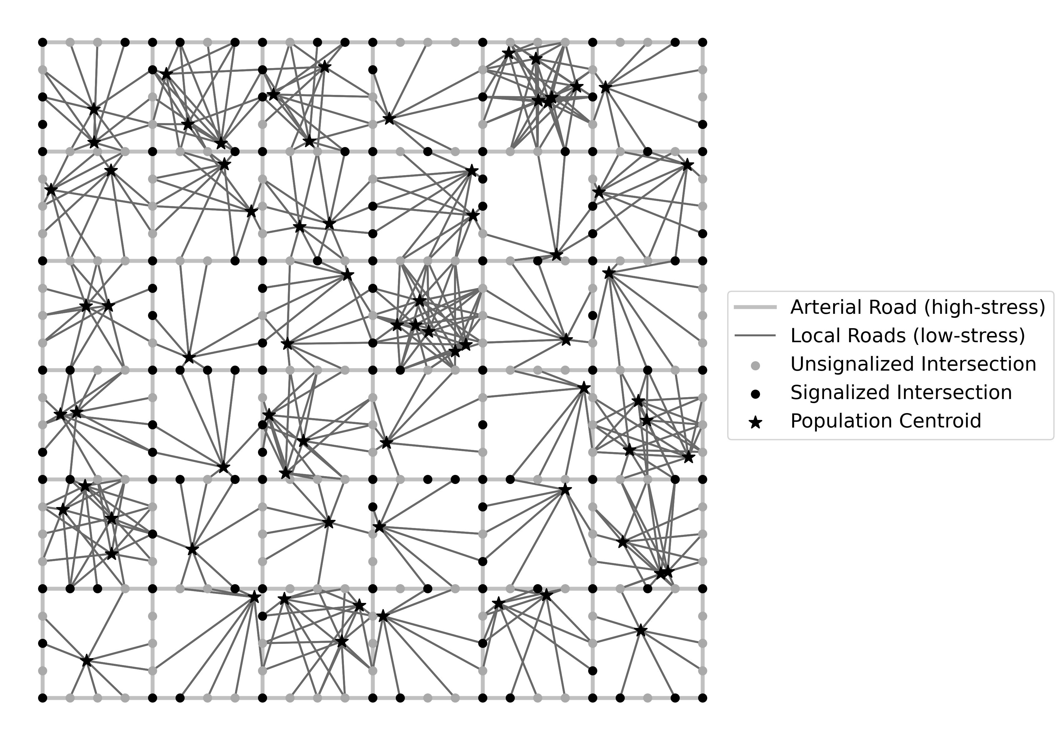
Figure 7: A synthetic grid network. Network components that are highlighted in black or dark grey constitute a low-stress network while others are high-stress.

15.2 Accessibility Calculations

15.2.1 Location-based accessibility measures.

We vary the parameters of the piecewise linear function $g$, mimicing three commonly used impedance function for location-based accessibility (Figure 8):

1. Negative exponential function: $\beta_{1}=0.0375$, $\beta_{2}=0.00625$, $T_{1}=20$, $T_{2}=60$.

2. Linear function: $\beta_{1}=1/60$, $\beta_{2}=0$, $T_{1}=60$, $T_{2}=60$.

3. Rectangular function: $\beta_{1}=0.001$, $\beta_{2}=0.471$, $T_{1}=58$, $T_{2}=60$.

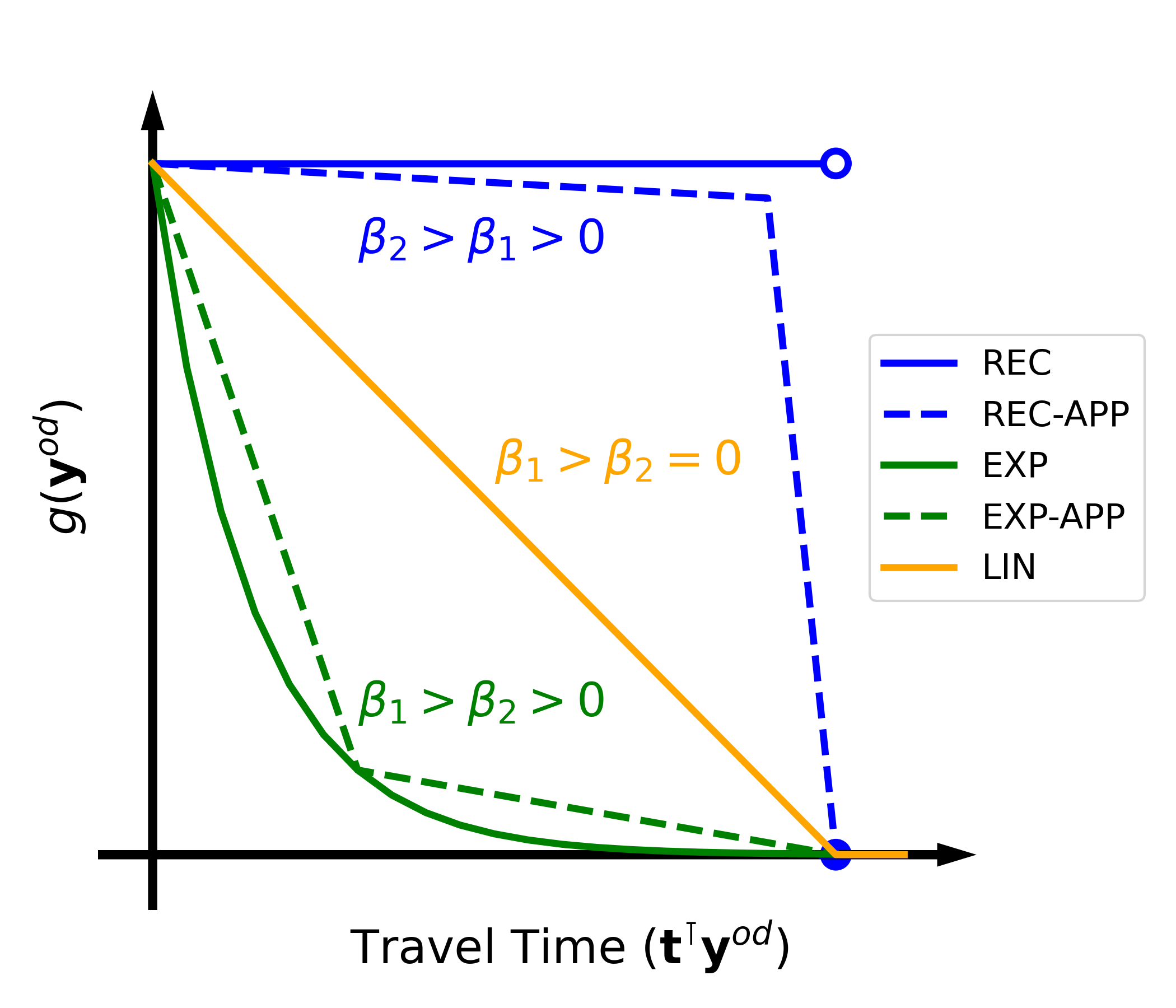
Figure 8: Negative exponential (EXP), rectangular (REC), and linear (LIN) impedance functions, and their piecewise linear approximations (APP).

15.2.2 Utility-based accessibility measure.

We adopt the utility-based measure proposed by Liu et al. (2022a). It requires as input a set of candidate routes for each OD pair and a constant $\alpha$ that reflects cyclists’ preference between bike-lane continuity and bike-lane coverage along the routes. Following Liu et al. (2022a), we set the value of $\alpha$ to $1.05$. We generate three candidate routes for each OD pair by solving three shortest path problems on the overall network using different edge travel cost. Specifically, we consider i) randomly generated travel time (Section 7), ii) Euclidean distance between the two ends, and iii) a uniform cost of 1 for all arterial roads and a uniform cost of 10 for other roads. The first and second definitions correspond to the goals of time minimization and distance minimization, both are commonly used by map software to generate route recommendations. The third definition reflects the preference for biking on major roads.

15.3 Predictive Features

15.3.1 Learned features.

We apply the representation learning technique introduced in Section 5 to learn OD-pair features for MaxANDP. Implementation details are illustrated as follows.

• Relationship Graph Construction. We sample $n_{\text{sim}}$ leader decisions for constructing the relationship graph. Ideally, the leader decisions should be sampled considering a specific design budget. However, the MaxANDP will be solved with various budgets in the computational studies (and in real-world transportation planning settings). Learning follower features multiple times may incur considerable computational burdens. Therefore, we consider learning features that are applicable to MaxANDP instances with different budgets by tweaking the leader decision sampling procedure. The high-level idea is to sample leader decisions with budgets randomly generated from a “wide” range that covers most budgets that may be used during the planning phase. As a result, the learned features contain information about follower similarity under various design budgets. Specifically, our leader-decision sampling procedure is parameterized by $\bar{P}$ and $\bar{Q}$ indicating, respectively, the maximum number of projects and the maximum number of nodes that can be selected in each sampled leader decision. Before generating a leader decision, we first randomly generate the number of projects and the number of nodes to be selected from intervals $[1,\bar{P}]$ and $[1,\bar{Q}]$, respectively. We then randomly select projects and nodes to form a leader decision. The procedure is summarized in Algorithm 3. In our computational studies, we set $\bar{P}=25$, $\bar{Q}=10$, and $n_{\text{sim}}$ = 5,000. We present computational results about the impact of $n_{\text{sim}}$ on feature quality in Section LABEL:appsub:exp1_emb_params.

• Follower Embedding. In our computational study, we set $n_{\text{walk}}=50$, $n_{\text{length}}=20$, $\omega=5$, and $\xi=16$. We investigate the impact of $\xi$ on feature quality in Section LABEL:appsub:exp1_emb_params.

Algorithm 3 Sampling leader’s decision for our cycling network design problem

Input: Number of decisions $n_{sim}$; Set of cycling infrastructure project $\mathcal{P}$; Set of high-stress nodes $\mathcal{N}_{h}$, Maximum number of infrastructure project selected $\bar{P}$; Maximum number of nodes selected $\bar{Q}$.
Output: A set of leader’s decisions $\bar{\mathcal{X}}$.

1:Initialize $\bar{\mathcal{X}}=\{\}$.

2:for $i=1$ to $n_{sim}$ do

3:     Generate $p\sim\textrm{Uniform}(1,\bar{P})$.

4:     Generate $q\sim\textrm{Uniform}(1,\bar{Q})$.

5:     Uniformly sample $\mathcal{P}_{i}\subseteq\mathcal{P}$ such that $|\mathcal{P}_{i}|=p$.

6:     Uniformly sample $\mathcal{Q}_{i}\subseteq\mathcal{N}_{h}$ such that $|\mathcal{Q}_{i}|=q$.

7:     Update $\bar{\mathcal{X}}\leftarrow\bar{\mathcal{X}}\cup\{(\mathcal{P}_{i},\mathcal{Q}_{i})\}$

References

- Alizadeh et al. (2013) Alizadeh S, Marcotte P, Savard G (2013) Two-stage stochastic bilevel programming over a transportation network. Transportation Research Part B: Methodological 58:92–105.
- Babier et al. (2023) Babier A, Chan TCY, Diamant A, Mahmood R (2023) Learning to optimize contextually constrained problems for real-time decision-generation. Management Science 0(0).
- Bagloee et al. (2016) Bagloee SA, Sarvi M, Wallace M (2016) Bicycle lane priority: Promoting bicycle as a green mode even in congested urban area. Transportation Research Part A: Policy and Practice 87:102–121.
- Ban and Rudin (2019) Ban GY, Rudin C (2019) The big data newsvendor: Practical insights from machine learning. Operations Research 67(1):90–108.
- Bao et al. (2017) Bao J, He T, Ruan S, Li Y, Zheng Y (2017) Planning bike lanes based on sharing-bikes’ trajectories. Proceedings of the 23rd ACM SIGKDD International Conference on Knowledge Discovery and Data Mining, 1377–1386.
- Bard (2013) Bard JF (2013) Practical bilevel optimization: algorithms and applications, volume 30 (Springer Science & Business Media).
- Bello et al. (2017) Bello I, Pham H, Le QV, Norouzi M, Bengio S (2017) Neural combinatorial optimization with reinforcement learning. International Conference on Learning Representations.
- Bengio et al. (2021) Bengio Y, Lodi A, Prouvost A (2021) Machine learning for combinatorial optimization: a methodological tour d’horizon. European Journal of Operational Research 290(2):405–421.
- Bergman et al. (2022) Bergman D, Huang T, Brooks P, Lodi A, Raghunathan AU (2022) Janos: an integrated predictive and prescriptive modeling framework. INFORMS Journal on Computing 34(2):807–816.
- Bertsimas and Kallus (2020) Bertsimas D, Kallus N (2020) From predictive to prescriptive analytics. Management Science 66(3):1025–1044.
- Bertsimas and Mundru (2023) Bertsimas D, Mundru N (2023) Optimization-based scenario reduction for data-driven two-stage stochastic optimization. Operations Research 71(4):1343–1361.
- Biggs et al. (2017) Biggs M, Hariss R, Perakis G (2017) Optimizing objective functions determined from random forests, available at SSRN: https://ssrn.com/abstract=2986630.
- Birge and Louveaux (2011) Birge JR, Louveaux F (2011) Introduction to stochastic programming (Springer Science & Business Media).
- Bodur and Luedtke (2017) Bodur M, Luedtke JR (2017) Mixed-integer rounding enhanced benders decomposition for multiclass service-system staffing and scheduling with arrival rate uncertainty. Management Science 63(7):2073–2091.
- Boutilier and Chan (2020) Boutilier JJ, Chan TCY (2020) Ambulance emergency response optimization in developing countries. Operations Research 68(5):1315–1334.
- Buehler and Dill (2016) Buehler R, Dill J (2016) Bikeway networks: A review of effects on cycling. Transport Reviews 36(1):9–27.
- Buehler and Pucher (2021) Buehler R, Pucher J (2021) COVID-19 impacts on cycling, 2019–2020. Transport Reviews 41(4):393–400.
- Candler and Townsley (1982) Candler W, Townsley R (1982) A linear two-level programming problem. Computers & Operations Research 9(1):59–76.
- Carlsson (2012) Carlsson JG (2012) Dividing a territory among several vehicles. INFORMS Journal on Computing 24(4):565–577.
- Carlsson and Jones (2022) Carlsson JG, Jones B (2022) Continuous approximation formulas for location problems. Networks 80(4):407–430.
- Carrión et al. (2009) Carrión M, Arroyo JM, Conejo AJ (2009) A bilevel stochastic programming approach for retailer futures market trading. IEEE Transactions on Power Systems 24(3):1446–1456.
- Chen et al. (2008) Chen X, Sim M, Sun P, Zhang J (2008) A linear decision-based approximation approach to stochastic programming. Operations Research 56(2):344–357.
- City of Toronto (2020) City of Toronto (2020) City of Toronto open data. https://www.toronto.ca/city-government/data-research-maps/open-data/, accessed: 2020-09-15.
- City of Toronto (2021a) City of Toronto (2021a) 2021 cycling network plan update. Accessed via https://www.toronto.ca/legdocs/mmis/2021/ie/bgrd/backgroundfile-173663.pdf on July 8, 2022.
- City of Toronto (2021b) City of Toronto (2021b) ActiveTO: Lessons learned from 2020 and next steps for 2021. Accessed via https://www.toronto.ca/legdocs/mmis/2021/ie/bgrd/backgroundfile-164864.pdf on July 21, 2022.
- City of Toronto (2021c) City of Toronto (2021c) Cycling network plan update — external stakeholders briefing summary. Accessed via https://www.toronto.ca/wp-content/uploads/2021/06/8ea2-External-Briefing-Meeting-Summary-June-7-2021.pdf on July 21, 2022.
- Cleveland and Devlin (1988) Cleveland WS, Devlin SJ (1988) Locally weighted regression: an approach to regression analysis by local fitting. Journal of the American Statistical Association 83(403):596–610.
- Crainic et al. (2014) Crainic TG, Hewitt M, Rei W (2014) Scenario grouping in a progressive hedging-based meta-heuristic for stochastic network design. Computers & Operations Research 43:90–99.
- Devlin et al. (2019) Devlin J, Chang M, Lee K, Toutanova K (2019) BERT: pre-training of deep bidirectional transformers for language understanding. Proceedings of the 2019 Conference of the North American Chapter of the Association for Computational Linguistics: Human Language Technologies, NAACL-HLT, 4171–4186.
- Dill and McNeil (2016) Dill J, McNeil N (2016) Revisiting the four types of cyclists: Findings from a national survey. Transportation Research Record 2587(1):90–99.
- Dupačová et al. (2003) Dupačová J, Gröwe-Kuska N, Römisch W (2003) Scenario reduction in stochastic programming. Mathematical Programming 95(3):493–511.
- Duthie and Unnikrishnan (2014) Duthie J, Unnikrishnan A (2014) Optimization framework for bicycle network design. Journal of Transportation Engineering 140(7):04014028.
- Elmachtoub and Grigas (2022) Elmachtoub AN, Grigas P (2022) Smart “predict, then optimize”. Management Science 68(1):9–26.
- Fampa et al. (2008) Fampa M, Barroso L, Candal D, Simonetti L (2008) Bilevel optimization applied to strategic pricing in competitive electricity markets. Computational Optimization and Applications 39(2):121–142.
- Ferreira et al. (2016) Ferreira KJ, Lee BHA, Simchi-Levi D (2016) Analytics for an online retailer: Demand forecasting and price optimization. Manufacturing & Service Operations Management 18(1):69–88.
- Fischetti et al. (2017) Fischetti M, Ljubić I, Sinnl M (2017) Redesigning benders decomposition for large-scale facility location. Management Science 63(7):2146–2162.
- Furth et al. (2016) Furth PG, Mekuria MC, Nixon H (2016) Network connectivity for low-stress bicycling. Transportation Research Record 2587(1):41–49.
- Furth et al. (2018) Furth PG, Putta TV, Moser P (2018) Measuring low-stress connectivity in terms of bike-accessible jobs and potential bike-to-work trips. Journal of Transport and Land Use 11(1):815–831.
- Gehrke et al. (2020) Gehrke SR, Akhavan A, Furth PG, Wang Q, Reardon TG (2020) A cycling-focused accessibility tool to support regional bike network connectivity. Transportation Research Part D: Transport and Environment 85:102388.
- Geurs and Van Wee (2004) Geurs KT, Van Wee B (2004) Accessibility evaluation of land-use and transport strategies: review and research directions. Journal of Transport Geography 12(2):127–140.
- Gonzalez (1985) Gonzalez TF (1985) Clustering to minimize the maximum intercluster distance. Theoretical Computer Science 38:293–306.
- Gurobi Optimization, LLC (2022) Gurobi Optimization, LLC (2022) Gurobi Optimizer Reference Manual. URL https://www.gurobi.com.
- Harkey et al. (1998) Harkey DL, Reinfurt DW, Knuiman M (1998) Development of the bicycle compatibility index. Transportation Research Record 1636(1):13–20.
- Hewitt et al. (2021) Hewitt M, Ortmann J, Rei W (2021) Decision-based scenario clustering for decision-making under uncertainty. Annals of Operations Research 1–25.
- Hochbaum and Shmoys (1985) Hochbaum DS, Shmoys DB (1985) A best possible heuristic for the k-center problem. Mathematics of Operations Research 10(2):180–184.
- Hoeffding (1994) Hoeffding W (1994) Probability inequalities for sums of bounded random variables. The Collected Works of Wassily Hoeffding, 409–426 (Springer).
- Iacono et al. (2010) Iacono M, Krizek KJ, El-Geneidy A (2010) Measuring non-motorized accessibility: issues, alternatives, and execution. Journal of Transport Geography 18(1):133–140.
- Imani et al. (2019) Imani AF, Miller EJ, Saxe S (2019) Cycle accessibility and level of traffic stress: A case study of Toronto. Journal of Transport Geography 80:102496.
- Jia and Shen (2021) Jia H, Shen S (2021) Benders cut classification via support vector machines for solving two-stage stochastic programs. INFORMS Journal on Optimization 3(3):278–297.
- Kent and Karner (2019) Kent M, Karner A (2019) Prioritizing low-stress and equitable bicycle networks using neighborhood-based accessibility measures. International Journal of Sustainable Transportation 13(2):100–110.
- Keutchayan et al. (2023) Keutchayan J, Ortmann J, Rei W (2023) Problem-driven scenario clustering in stochastic optimization. Computational Management Science 20(1):13.
- Khalil et al. (2017) Khalil E, Dai H, Zhang Y, Dilkina B, Song L (2017) Learning combinatorial optimization algorithms over graphs. Advances in Neural Information Processing Systems, 6348–6358.
- Khalil et al. (2016) Khalil E, Le Bodic P, Song L, Nemhauser G, Dilkina B (2016) Learning to branch in mixed integer programming. Proceedings of the AAAI Conference on Artificial Intelligence, volume 30.
- Kool et al. (2019) Kool W, van Hoof H, Welling M (2019) Attention, learn to solve routing problems! International Conference on Learning Representations.
- Kotary et al. (2021) Kotary J, Fioretto F, Van Hentenryck P, Wilder B (2021) End-to-end constrained optimization learning: A survey. arXiv preprint arXiv:2103.16378 .
- Kou et al. (2020) Kou Z, Wang X, Chiu SFA, Cai H (2020) Quantifying greenhouse gas emissions reduction from bike share systems: a model considering real-world trips and transportation mode choice patterns. Resources, Conservation and Recycling 153:104534.
- Kraus and Koch (2021) Kraus S, Koch N (2021) Provisional COVID-19 infrastructure induces large, rapid increases in cycling. Proceedings of the National Academy of Sciences 118(15).
- Landis et al. (1997) Landis BW, Vattikuti VR, Brannick MT (1997) Real-time human perceptions: toward a bicycle level of service. Transportation Research Record 1578(1):119–126.
- Larsen et al. (2013) Larsen J, Patterson Z, El-Geneidy A (2013) Build it. but where? the use of geographic information systems in identifying locations for new cycling infrastructure. International Journal of Sustainable Transportation 7(4):299–317.
- Leal et al. (2020) Leal M, Ponce D, Puerto J (2020) Portfolio problems with two levels decision-makers: Optimal portfolio selection with pricing decisions on transaction costs. European Journal of Operational Research 284(2):712–727.
- Lewis and Gale (1994) Lewis DD, Gale WA (1994) A sequential algorithm for training text classifiers. SIGIR’94, 3–12.
- Li et al. (2017) Li S, Muresan M, Fu L (2017) Cycling in Toronto, Ontario, Canada: Route choice behavior and implications for infrastructure planning. Transportation Research Record 2662(1):41–49.
- Lim et al. (2021) Lim J, Dalmeijer K, Guhathakurta S, Van Hentenryck P (2021) The bicycle network improvement problem: Optimization algorithms and a case study in Atlanta. Journal of Transportation Engineering, Part A: Systems 148(11).
- Lin et al. (2021) Lin B, Chan TCY, Saxe S (2021) The impact of COVID-19 cycling infrastructure on low-stress cycling accessibility: A case study in the City of Toronto. Findings 19069.
- Liu et al. (2019) Liu H, Szeto W, Long J (2019) Bike network design problem with a path-size logit-based equilibrium constraint: Formulation, global optimization, and matheuristic. Transportation Research Part E: Logistics and Transportation Review 127:284–307.
- Liu et al. (2021) Liu S, He L, Shen ZJM (2021) On-time last-mile delivery: Order assignment with travel-time predictors. Management Science 67(7):4095–4119.
- Liu et al. (2022a) Liu S, Shen ZJM, Ji X (2022a) Urban bike lane planning with bike trajectories: Models, algorithms, and a real-world case study. Manufacturing & Service Operations Management 24(5):2500–2515.
- Liu et al. (2022b) Liu S, Siddiq A, Zhang J (2022b) Planning bike lanes with data: Ridership, congestion, and path selection, available at SSRN: https://ssrn.com/abstract=4055703.
- Lowry et al. (2012) Lowry MB, Callister D, Gresham M, Moore B (2012) Assessment of communitywide bikeability with bicycle level of service. Transportation Research Record 2314(1):41–48.
- Magnanti et al. (1986) Magnanti TL, Mireault P, Wong RT (1986) Tailoring benders decomposition for uncapacitated network design. Netflow at Pisa, 112–154 (Springer).
- Mauttone et al. (2017) Mauttone A, Mercadante G, Rabaza M, Toledo F (2017) Bicycle network design: model and solution algorithm. Transportation Research Procedia 27:969–976.
- McGivney and Yukich (1999) McGivney K, Yukich J (1999) Asymptotics for geometric location problems over random samples. Advances in Applied Probability 31(3):632–642.
- Mesbah et al. (2012) Mesbah M, Thompson R, Moridpour S (2012) Bilevel optimization approach to design of network of bike lanes. Transportation Research Record 2284(1):21–28.
- Mikolov et al. (2013) Mikolov T, Sutskever I, Chen K, Corrado GS, Dean J (2013) Distributed representations of words and phrases and their compositionality. Advances in Neural Information Processing Systems, volume 26.
- Mišić (2020) Mišić VV (2020) Optimization of tree ensembles. Operations Research 68(5):1605–1624.
- Morabit et al. (2021) Morabit M, Desaulniers G, Lodi A (2021) Machine-learning–based column selection for column generation. Transportation Science 55(4):815–831.
- Mueller et al. (2018) Mueller N, Rojas-Rueda D, Salmon M, Martinez D, Ambros A, Brand C, De Nazelle A, Dons E, Gaupp-Berghausen M, Gerike R, et al. (2018) Health impact assessment of cycling network expansions in european cities. Preventive Medicine 109:62–70.
- Naoum-Sawaya and Elhedhli (2013) Naoum-Sawaya J, Elhedhli S (2013) An interior-point benders based branch-and-cut algorithm for mixed integer programs. Annals of Operations Research 210(1):33–55.
- Nazari et al. (2018) Nazari M, Oroojlooy A, Snyder L, Takác M (2018) Reinforcement learning for solving the vehicle routing problem. Advances in Neural Information Processing Systems, 9839–9849.
- Notz and Pibernik (2022) Notz PM, Pibernik R (2022) Prescriptive analytics for flexible capacity management. Management Science 68(3):1756–1775.
- Olmos et al. (2020) Olmos LE, Tadeo MS, Vlachogiannis D, Alhasoun F, Alegre XE, Ochoa C, Targa F, González MC (2020) A data science framework for planning the growth of bicycle infrastructures. Transportation Research Part C: Emerging Technologies 115:102640.
- Ospina et al. (2022) Ospina JP, Duque JC, Botero-Fernández V, Montoya A (2022) The maximal covering bicycle network design problem. Transportation Research part A: Policy and Practice 159:222–236.
- Papadakos (2008) Papadakos N (2008) Practical enhancements to the Magnanti-Wong method. Operations Research Letters 36(4):444–449.
- Parzen (1962) Parzen E (1962) On estimation of a probability density function and mode. The Annals of Mathematical Statistics 33(3):1065–1076.
- Patel et al. (2022) Patel RM, Dumouchelle J, Khalil E, Bodur M (2022) Neur2SP: Neural two-stage stochastic programming. Advances in Neural Information Processing Systems, volume 35, 23992–24005.
- Pedregosa et al. (2011) Pedregosa F, Varoquaux G, Gramfort A, Michel V, Thirion B, Grisel O, Blondel M, Prettenhofer P, Weiss R, Dubourg V, Vanderplas J, Passos A, Cournapeau D, Brucher M, Perrot M, Duchesnay E (2011) Scikit-learn: Machine learning in Python. Journal of Machine Learning Research 12:2825–2830.
- Perozzi et al. (2014) Perozzi B, Al-Rfou R, Skiena S (2014) Deepwalk: Online learning of social representations. Proceedings of the 20th ACM SIGKDD International Conference on Knowledge Discovery and Data Mining, 701–710.
- Prochazka and Wallace (2020) Prochazka V, Wallace SW (2020) Scenario tree construction driven by heuristic solutions of the optimization problem. Computational Management Science 17(2):277–307.
- Putta and Furth (2019) Putta T, Furth PG (2019) Method to identify and visualize barriers in a low-stress bike network. Transportation Research Record 2673(9):452–460.
- Radford et al. (2018) Radford A, Narasimhan K, Salimans T, Sutskever I, et al. (2018) Improving language understanding by generative pre-training. Preprint: https://openai.com/research/language-unsupervised .
- Řehůřek and Sojka (2010) Řehůřek R, Sojka P (2010) Software Framework for Topic Modelling with Large Corpora. Proceedings of the LREC 2010 Workshop on New Challenges for NLP Frameworks, 45–50.
- Römisch and Schultz (1991) Römisch W, Schultz R (1991) Stability analysis for stochastic programs. Annals of Operations Research 30(1):241–266.
- Römisch and Wets (2007) Römisch W, Wets RB (2007) Stability of -approximate solutions to convex stochastic programs. SIAM Journal on Optimization 18(3):961–979.
- Saghapour et al. (2017) Saghapour T, Moridpour S, Thompson RG (2017) Measuring cycling accessibility in metropolitan areas. International Journal of Sustainable Transportation 11(5):381–394.
- Sener and Savarese (2018) Sener O, Savarese S (2018) Active learning for convolutional neural networks: A core-set approach. International Conference on Learning Representations.
- Settles (2009) Settles B (2009) Active learning literature survey. Computer Sciences Technical Report 1648, University of Wisconsin–Madison.
- Settles et al. (2007) Settles B, Craven M, Ray S (2007) Multiple-instance active learning. Proceedings of the Twenty-First Annual Conference on Neural Information Processing Systems, 1289–1296.
- Shapiro et al. (2009) Shapiro A, Dentcheva D, Ruszczynski A (2009) Lectures on stochastic programming: modeling and theory (SIAM).
- Sisson et al. (2006) Sisson SB, Lee SM, Burns EK, Tudor-Locke C (2006) Suitability of commuting by bicycle to Arizona elementary schools. American Journal of Health Promotion 20(3):210–213.
- Sohn (2011) Sohn K (2011) Multi-objective optimization of a road diet network design. Transportation Research Part A: Policy and Practice 45(6):499–511.
- Song et al. (2020) Song J, lanka r, Yue Y, Dilkina B (2020) A general large neighborhood search framework for solving integer linear programs. Advances in Neural Information Processing Systems, volume 33, 20012–20023 (Curran Associates, Inc.).
- Statistics Canada (2016a) Statistics Canada (2016a) Dissemination area boundary files. https://www150.statcan.gc.ca/n1/en/catalogue/92-169-X#, accessed: 2020-11-15.
- Statistics Canada (2016b) Statistics Canada (2016b) Population and dwelling count, 2016 census. https://www12.statcan.gc.ca/census-recensement/2016/dp-pd/hlt-fst/pd-pl/Table.cfm?Lang=Eng&T=1902&PR=35&S=3&O=D&RPP=50, accessed: 2020-11-15.
- Stroh et al. (2022) Stroh AM, Erera AL, Toriello A (2022) Tactical design of same-day delivery systems. Management Science 68(5):3444–3463.
- Tang et al. (2020) Tang Y, Agrawal S, Faenza Y (2020) Reinforcement learning for integer programming: Learning to cut. International Conference on Machine Learning, 9367–9376 (PMLR).
- Vale et al. (2016) Vale DS, Saraiva M, Pereira M (2016) Active accessibility: A review of operational measures of walking and cycling accessibility. Journal of Transport and Land Use 9(1):209–235.
- Van Hoesel (2008) Van Hoesel S (2008) An overview of stackelberg pricing in networks. European Journal of Operational Research 189(3):1393–1402.
- Vinyals et al. (2015) Vinyals O, Fortunato M, Jaitly N (2015) Pointer networks. Advances in Neural Information Processing Systems, 2692–2700.
- White and Anandalingam (1993) White DJ, Anandalingam G (1993) A penalty function approach for solving bi-level linear programs. Journal of Global Optimization 3(4):397–419.
- Wu et al. (2022) Wu Y, Song W, Cao Z, Zhang J (2022) Learning scenario representation for solving two-stage stochastic integer programs. International Conference on Learning Representations.
- Zetina et al. (2019) Zetina CA, Contreras I, Cordeau JF (2019) Exact algorithms based on benders decomposition for multicommodity uncapacitated fixed-charge network design. Computers & Operations Research 111:311–324.
- Zhang et al. (2023) Zhang W, Wang K, Jacquillat A, Wang S (2023) Optimized scenario reduction: Solving large-scale stochastic programs with quality guarantees. INFORMS Journal on Computing .
- Zugno et al. (2013) Zugno M, Morales JM, Pinson P, Madsen H (2013) A bilevel model for electricity retailers’ participation in a demand response market environment. Energy Economics 36:182–197.