A Dynamic Stochastic Block Model for Multi–Layer Networks

Abstract

We propose a flexible stochastic block model for multi–layer networks, where layer–specific hidden Markov–chain processes drive the changes in the formation of communities. The changes in block membership of a node in a given layer may be influenced by its own past membership in other layers. This allows for clustering overlap, clustering decoupling, or more complex relationships between layers including settings of unidirectional, or bidirectional, block causality. We cope with the overparameterization issue of a saturated specification by assuming a Multi–Laplacian prior distribution within a Bayesian framework. Data augmentation and Gibbs sampling are used to make the inference problem more tractable. Through simulations, we show that the standard linear models are not able to detect the block causality under the great majority of scenarios. As an application to trade networks, we show that our model provides a unified framework including community detection and Gravity equation. The model is used to study the causality between trade agreements and trade looking at the global topological properties of the networks as opposed to the main existent approaches which focus on local bilateral relationships. We are able to provide new evidence of unidirectional causality from the free trade agreements network to the non–observable trade barriers network structure for 159 countries in the period 1995–2017.

Keywords: stochastic block model; hidden Markov chain; multi–layer network; edge clustering; Granger causality; group LASSO; FTAs effectiveness; Gravity equation.

1 Introduction

Network models are as a tool to study real-world complex systems and as an alternative to extreme reductionist approaches [28, 82, 11, e.g., see]. They have become a convenient framework to describe social and economic interactions and have attracted theorists and applied researchers [23, 62, see for example]. In terms of higher–order network properties, such as clustering, several stochastic models have been proposed apart from the exponential random graphs, e.g. latent space models and stochastic block models, from now on Stochastic Block Model (SBM) [51, 40]. However, in systems with multiple types of interactions between nodes, a single graph does not fully describe the connectivity structure, thus graphs with multiple–type of edges (layers) have been introduced. See [6, 53, 57] for an introduction to multi–layer networks. To the best of our knowledge, relatively few works deal with dynamic clustering models for multi–layer graphs [56, 69, 58]. The objective of the present work is to provide an extension to the dynamic SBM (DSBM) to accounts for multiple edges types.

In SBM modelling, edge clustering is driven by a probabilistic classification of the nodes into different communities. In a dynamic setting, it involves the use of Hidden Markov Chains (HMCs) to capture temporal changes in the node’s membership. [84] work with (un)directed and unweighted networks and [62] generalize their model to include weighted networks and discuss the identification issues when block–dependent connectivity parameters are time–varying. Other extensions deal with mixed membership and the heterogeneity of connectivity parameters across nodes [3, 86].

In these previous works, the DSBM has accounted for one type of edges. However, in the context of social and economic relationships, usually there is more than one type of ties, such as multiple goods traded between regions, or several assets exchanged by financial institutions [12, 73]. Therefore, we propose a DSBM for multi–layer networks (DSBMM) where each type of relationship is represented by a different layer, with no inter–layer edges and time–invariant and layer–invariant node set [4].

To the best of our knowledge, extensions of the SBM in a multi–layer setting are static and correlational. [47] identify communities per layer (local clustering), and a consensus of all layers (global clustering) with unweighted edges. [78] in a static framework consider a SBM for each layer, and propose to cluster similar layers, so they can share a common SBM. Other studies with no interest on community detection use multivariate distributions to make inference on the dependence between layers, but this restricts all layers to be of the same type, that is either weighted or unweighted and directed or undirected [12]. These alternatives in a multi–layer context provide a measure of association or clustering overlap between layers, but it is not possible to infer if the nature of the relationship is unidirectional or bidirectional.

Our DSBMM introduces a concept of nonlinear Granger–block causality, which identify the directed dependence between layers’ community structure. For instance, layer $\ell$ may be Granger–block causing layer $\mathfrak{m}$, but not vice–versa. Specifically, in the DSBMM, the nodes membership dynamic in each layer is influenced by their respective membership in the rest of layers. In contrast to the applications in the Markov–switching literature, the DSBMM is more general because the number of states can vary between layers and may include more than two states. In this way, by using a saturated multinomial specification to model the transition matrix of each layer, it is possible to test for Granger causality between layers. The approach also allows layers of different type, i.e. (un)directed or (un)weighted and a set of layer–specific covariates to control for observed node or dyad heterogeneity.

We follow a Bayesian inference approach and propose a full Gibbs sampler to approximate the posterior distributions of the parameters by using a Pólya Gamma representation of the multinomial model [71]. Given the large number of transition parameters in the saturated model, a Multi–Laplacian prior is introduced to induce a group LASSO penalty that relies on data augmentation to keep tractability [72]. Our simulations results show that the Multi–Laplacian prior performs better than a normal prior and more importantly that benchmark models such as the standard Bayesian Vector Autoregression (BVAR) models are not able to detect the Granger–block causality under the great majority of scenarios.

We apply our DSBMM model to trade flows and free trade agreements (FTA) and contribute to the debate on the effectiveness of FTA as a policy instrument for global trade integration [8, 9]. The wide range of estimates of FTA effect on trade and the complexity of overlapping FTA between countries suggest that the consideration of the network structure can provide a complementary view of the FTA effect on the topological properties of the trade flows. In this sense, we test if FTA clustering has an impact on the international trade community membership after controlling for country and dyad observed heterogeneity. Community detection in the international trade flows have been analyzed mainly using only a modularity approach. For example, [14] focuses on the aggregate trade flows to infer the groups of countries with a dense connectivity and [13] uses commodity-specific layers and identify communities of countries per product, both contributions perform their task by maximizing a modularity function through numerical methods. Our statistical model approach for community detection, accounts for uncertainty in the parameters and community membership. Moreover, by allowing covariates affecting trade flows, our DSBMM integrates community detection into Gravity equation models, extensively used in international trade [70, e.g.]. The paper is organized as follows. Section 2 introduces the DSBMM and presents some numerical illustrations of the model properties. In Section 3 addresses the inference procedure, including the choice of prior distribution, the details of the Gibbs sampler, and a comparison with BVAR models in terms of causality detection with synthetic data. Section 4 provides an application to the Trade Flows–FTAs multi–layer network. Section 5 summarizes the main conclusions.

2 A Dynamic SBM for multi–layer networks

2.1 Multi–Layer DSBM

A graph can be defined as the ordered triplet $\mathcal{G}=(\mathcal{V},\mathcal{E},Y)$, where the node set $\mathcal{V}=\{1,\cdots,N\}$ is the same across the layer set $\mathcal{L}=\{1,\ldots,L\}$ and the edge set collection $\mathcal{E}=(\mathcal{E}^{(1)},\ldots,\mathcal{E}^{(L)})$, $\mathcal{E}^{(\ell)}\subseteq\mathcal{V}\times\mathcal{V}$ allows only for intra–layer edges. The set $Y=\{Y^{(1)},\cdots,Y^{(L)}\}$ includes the layer–specific adjacency matrices with $Y^{(\ell)}\in\mathbb{R}^{N}\times\mathbb{R}^{N}$ where the $(i,j)$–th element of $Y^{(\ell)}$ is $Y^{(\ell)}_{ij}=0$ if $(i,j)\not\in\mathcal{E}^{(\ell)}$ and $Y^{(\ell)}_{ij}=a\in\mathbb{R}\backslash\{0\}$ if $(i,j)\in\mathcal{E}^{(\ell)}$. The multi–layer may jointly consider (un)directed and (un)weighted layers resulting in (a)symmetric and (binary) real valued adjacency matrices.

Considering that clustering and higher–order network structures, such as clubs or closed communities, are common features in real–world graphs [21, e.g.,], a SBM can be used in each layer to model edge clustering through node grouping. We define the set $\mathfrak{V}=\{\mathfrak{V}^{(1)},\dots,\mathfrak{V}^{(L)}\}$, where each element is a layer–specific partition of the node set into $Q^{(\ell)}$ subsets, that is, $\mathfrak{V}^{(\ell)}=\{\mathcal{V}^{(\ell)}_{1},\ldots,\mathcal{V}^{(\ell)}_{Q^{(\ell)}}\}$ and each $\mathcal{V}^{(\ell)}_{q}\subseteq\mathcal{V}$ is called block or community in layer $\ell$, satisfying two properties: $\mathcal{V}^{(\ell)}_{q}\cap\mathcal{V}^{(\ell)}_{r}=\emptyset$, $q\neq r$, and $\cup_{q\in\mathcal{Q}^{(\ell)}}\mathcal{V}^{(l)}_{q}=\mathcal{V},\ \mathcal{Q}^{(\ell)}=\{1,\dots,Q^{(\ell)}\}$.

It is assumed that the multi–layer graph evolves over time, $\mathcal{G}_{1:T}=\{\mathcal{G}_{t}\}_{t\in\mathcal{T}}$, with $\mathcal{G}_{t}=(\mathcal{V},\mathcal{E}_{t},Y_{t})$, $\mathcal{T}=\{1,\ldots,T\}$, and a latent sequence of partitions $\mathfrak{V}_{1:T}=\{\mathfrak{V}_{t}\}_{t\in\mathcal{T}}$ drives its topology. For a layer $\ell$, the block membership of a node is indicated by the latent variable $Z^{(\ell)}_{it}=q\in\mathcal{Q}^{(\ell)}$, for $t\in\mathcal{T}$. Notice that the partition sequence and the memberships are intrinsically related $\mathcal{V}_{qt}^{(\ell)}=\{i\in\mathcal{V}|Z^{(\ell)}_{it}=q\}$. Then, the membership dynamics $Z^{(\ell)}_{i}=\{Z^{(\ell)}_{i1},\dots,Z^{(\ell)}_{iT}\}$, follows a hidden Markov–chain process. Specifically, for the initial membership $Z^{(\ell)}_{i1}$, the probabilities of belonging to a block are collected into the vector $\alpha^{(\ell)}=\{\alpha^{(\ell)}_{1},\dots,\alpha^{(\ell)}_{Q^{(\ell)}}\}$, where $\sum_{q\in\mathcal{Q}^{(\ell)}}\alpha^{(\ell)}_{q}=1$. The membership changes for $t\in\mathcal{T}\backslash\{1\}$ are determined by the transition matrix $P_{it}^{(\ell)}$, where $P^{(\ell)}_{it,qr}\in(0,1)$ for $q,r\in\mathcal{Q}^{(\ell)}$ and $\sum_{r\in\mathcal{Q}^{(\ell)}}P^{(\ell)}_{it,qr}=1$. The transition probabilities vary across nodes and time, because they depend on the node’s previous membership in all the layers, i.e. $Z^{(1:L)}_{it-1}$, allowing for inter–layer dependence.

The contemporaneous network $Y^{(\ell)}_{t}$ only depends on $Z^{(\ell)}_{t}=\{Z^{(\ell)}_{1t},\dots,Z^{(\ell)}_{Nt}\}$ and layer–specific covariates $X^{(\ell)}_{1:T}$, i.e. given $Z^{(\ell)}_{1:T}$ and $X^{(\ell)}_{ijt}$, $Y^{(\ell)}_{1:T}$ components are independent. Each entry of the $\ell$–th adjacency matrix follows the mixed distribution,

$$Y_{ijt}^{(\ell)}\left|X^{(\ell)}_{ijt},Z^{(\ell)}_{it}=q,Z^{(\ell)}_{jt}=r,\vartheta^{(\ell)}\right.\sim(1-\nu^{(\ell)}_{qr})\delta(y)+\nu^{(\ell)}_{qr}f^{(\ell)}\left(y|\theta^{(\ell)}_{qr},X^{(\ell)}_{ijt}\right)$$ (1)

where $\vartheta^{(\ell)}=\left(\nu^{(\ell)},\theta^{(\ell)^{\prime}}\right)^{\prime}$ is the parameter vector, $\delta(\cdot)$ denotes the Dirac function at zero, and $f^{(\ell)}(\cdot|\theta^{(\ell)}_{qr},X^{(\ell)}_{ijt})$ is a layer–specific probability density function with parameters $\theta^{(\ell)}_{qr}$. Thus, the DSBMM extends the dynamic single–layer SBM [66] and the static SBM with observed heterogeneity [60] to a dynamic multi–layer set up with time–varying node or dyad characteristics, $X^{(\ell)}_{ijt}$. In other words, apart from introducing inter–layer dependence, in the one–layer case $L=1$, the DSBMM in (1) differs from [84, 62] in accounting for node or dyad observed heterogeneity through $X^{(\ell)}_{ijt}$. This can be interpreted as a regression with parameters partially pooled across dyads and time. Consequently, (1) is more flexible than a standard fixed parameters regression, and more feasible and parsimonious than a time–dyad varying case $\vartheta_{ijt}^{(\ell)}$.

Let $D_{ijt}^{(\ell)}$ be an indicator variable such that $D_{ijt}^{(\ell)}=1$ if $(i,j)\in\mathcal{E}_{t}^{(\ell)}$ and $D_{ijt}^{(\ell)}=0$ if $(i,j)\not\in\mathcal{E}_{t}^{(\ell)}$, then (1) can be rewritten as

$$Y^{(\ell)}_{ijt}\left|X^{(\ell)}_{ijt},D^{(\ell)}_{ijt},Z^{(\ell)}_{it}=q,Z^{(\ell)}_{jt}=r,\vartheta^{(\ell)}\right.\sim\left\{\begin{array}[]{ll}\delta(y)&\text{ if }D^{(\ell)}_{ijt}=0\\ f^{(\ell)}\left(y|\theta^{(\ell)}_{qr},X^{(\ell)}_{ijt}\right)&\text{ if }D^{(\ell)}_{ijt}=1\end{array}\right.$$ (2)

where the indicator variable follows a Bernoulli distribution:

$$D^{(\ell)}_{ijt}\left|X^{(\ell)}_{ijt},Z^{(\ell)}_{it}=q,Z^{(\ell)}_{jt}=r,\vartheta^{(\ell)}\right.\sim\operatorname{Bern}\left(\nu^{(\ell)}_{qr}\right)$$ (3)

The advantage of this representation is twofold. First, in this paper we assume that $Y^{(\ell)}_{ijt}=0$ indicates the absence of an edge and not a missing value and that $D^{(\ell)}_{ijt}$ is observable. Nevertheless, the model in (2) and (3) can be easily extended to account for missing values and latent indicator variables following a Heckman procedure [37, 81]. Second, (3) accounts for both weighted and unweighted layer. In case of unweighted layers, equations (2) and (3) simplify to (3), which allow for regressors, i.e. $\tau\left(\nu^{(\ell)}_{qr}\right)=X^{(\ell)^{\prime}}_{ijt}\theta^{(\ell)}_{qr}$, where $\tau:(0,1)\to\mathbb{R}$ is a link function.

2.2 Dependent multi–layer DSBM

In alignment with the motivation of [36, 78, 47], a statistical model for multi–layer networks should also account for the edge redundancy, that is the persistence of edges between the same pair of nodes over the network layers, and more structurally, clustering redundancy. For instance, if a set of nodes is densely connected in one layer, a similar structure is highly likely in a second layer. Nevertheless, existing approaches are static, correlational and only account for clustering overlap. In order to capture dependence between the node partitions in the different layers including non–overlap dependence and identify a causal structure, we can exploit the time dimension and assume dependent Markov Chain processes [67, 17, 2].

We are interested in a Granger non–causality relation across layers, in this respect the transition probabilities for each layer only depend on the collection of memberships $\mathfrak{V}_{t-1}$, that is $Z^{(1:L)}_{it-1}=Z_{it-1}$. This assumption simplifies as follows the joint probability $\mathbb{P}(Z_{it}|Z_{it-1})$, $i\in\mathcal{V}$,

$$\mathbb{P}(Z_{it}|Z_{it-1})=\mathbb{P}\left(Z^{(1)}_{it}|Z_{it-1}\right)\prod_{\ell=2}^{L}\mathbb{P}\left(Z^{(\ell)}_{it}|Z^{(1:\ell-1)}_{it},Z_{it-1}\right)=\prod_{\ell=1}^{L}\mathbb{P}\left(Z^{(\ell)}_{it}|Z_{it-1}\right).$$ (4)

In contrast to the previous studies, which cover dependent Markov chains with two states only, the DSBMM requires a more general approach. Therefore, we use a multinomial logit form to express the Markov chain dependence through the transition matrix $\mathbb{P}\left(Z^{(\ell)}_{it}=q|Z_{it-1}\right)=P^{(\ell)}_{it,q},\ q=1,\dots,Q^{(\ell)}$ with $Q^{(\ell)}$ states. Similarly to the log–linear models used for contingency tables, $Z_{it-1}$ is represented by a full set of dummy variables, including the interactions and the main effects of the different layers [29, 1, e.g.,]. In other words, letting $W^{(\ell)}_{it,q}=\mathbb{I}_{\{q\}}\left(Z^{(\ell)}_{it}\right)$ and $W^{(\ell)}_{it}=\left(W^{(\ell)}_{it,1},\ldots,W^{(\ell)}_{it,Q^{(\ell)}-1}\right)^{\prime}$, then

$$\log\left(P^{(\ell)}_{it,q}C^{(\ell)}_{it}\right) =\kappa^{(\ell)}_{0,q}+\underbrace{\sum_{\mathfrak{m}=1}^{L}W^{(\mathfrak{m})^{\prime}}_{it-1}\kappa^{(\ell)}_{\mathfrak{m},q}}_{\text{main effects}}+\underbrace{\sum_{\mathfrak{m}>\mathfrak{n}}\left(W^{(\mathfrak{m})^{\prime}}_{it-1}\otimes W^{(\mathfrak{n})^{\prime}}_{it-1}\right)\kappa^{(\ell)}_{\mathfrak{m}\mathfrak{n},q}}_{\text{first order effects}}+\ldots+\underbrace{\bigotimes_{\mathfrak{m}=1}^{L}\left(W^{(\mathfrak{m})^{\prime}}_{it-1}\right)\kappa^{(\ell)}_{1\ldots L,q}}_{(L-1)\text{-th order effects}}$$ (5)

where $\kappa^{(\ell)}_{\mathcal{U},q}=\left(\kappa^{(\ell)}_{\mathcal{U},q,1},\ldots,\kappa^{(\ell)}_{\mathcal{U},q,s(\mathcal{U})}\right)^{\prime},\ \mathcal{U}\subseteq 2^{\mathcal{L}}$ and $s(\mathcal{U})=\prod_{\mathfrak{m}\in\mathcal{U}}\left(Q^{(\mathfrak{m})}-1\right)$. Equation (5) can be rewritten in an equivalent more compact form:

$$P^{(\ell)}_{it,q}=\frac{\exp\left(\widetilde{W}_{it-1}\kappa_{q}^{(\ell)}\right)}{\sum_{k=1}^{Q^{(\ell)}}\exp\left(\widetilde{W}_{it-1}\kappa_{k}^{(\ell)}\right)}$$ (6)

where $\widetilde{W}_{it-1}=\left(1,W^{(\ell)^{\prime}}_{it-1},\ldots,\bigotimes_{\mathfrak{m}=1}^{L}\left(W^{(\mathfrak{m})^{\prime}}_{it-1}\right)\right)$ and $\kappa_{q}^{(\ell)}=\left(\kappa^{(\ell)}_{0,q},\ldots,\kappa^{(\ell)^{\prime}}_{1\ldots L,q}\right)^{\prime}$ are a row and a column vector with $p+1$ elements, $p=\sum_{\mathcal{U}\subseteq 2^{\mathcal{L}}}s(\mathcal{U})$. For identification, $Z^{(\ell)}_{it}=Q^{(\ell)}$ can be used as reference state/community, i.e. $\kappa^{(\ell)}_{Q^{(\ell)}}=0$. This multivariate logistic specification is more flexible than the linear specification proposed by [2] for a panel Markov switching model because it does not have to impose any restriction on the parameters space of $\kappa_{q}^{(\ell)}$. As a consequence, (6) captures the special case of clustering overlap, but also more complex dependence structures, such as the decoupling one. In this modelling framework, it is straightforward to add other exogenous variables that affect membership and transition matrix [50, 41]. This flexibility in (6) comes at a cost of a lower tractability and a larger number of parameters. In this paper, we provide solution to both issues by a suitable inference approach.

The definition of non–causality introduced by [63] can be applied to the block membership processes. Let $\left\{Z_{t}=\left(Z^{(1)}_{t},\dots,Z^{(L)}_{t}\right)^{\prime},\ t\in\mathcal{T}\right\}$, or simply $\left\{Z_{t}\right\}$, in the triplet $\left(\Xi,\mathcal{A},\mathbb{P}\right)$. Then, an information set and a restricted information set are required to define a non–causality property. The available information up to time $t$, in terms of $\left\{Z_{t},S_{t}\right\}$, where $S_{t}$ is a set of exogenous variables, is referred as canonical filtration $\left\{\mathcal{F}_{t},\ t\in\mathcal{T}\right\}$, which is a sub–$\sigma$–algebra of $\mathcal{A}$. The reduced information sets are $\mathcal{R}^{(-\ell)}_{t}=\sigma((Z_{s}^{(-\ell)},S_{s}),\ 1\leq s\leq t)$ and $\mathcal{Z}^{(\ell)}_{t}=\sigma(Z_{s}^{(\ell)},\ 1\leq s\leq t)$, $\ell\in\mathcal{L}$, so that $\mathcal{Z}^{(\ell)}_{t}\subseteq\mathcal{R}^{(-\mathfrak{m})}_{t}\subseteq\mathcal{F}_{t}$ for all $\mathfrak{m}\neq\ell$.

Definition (Strong one–step ahead Granger–block non–causality).

$\{Z^{(\mathfrak{m})}_{t}\}$ does not strongly Granger–block cause $\{Z^{(\ell)}_{t}\}$ one–step ahead, and write $Z^{(\mathfrak{m})}\not\stackrel{{\scriptstyle G}}{{\Rightarrow}}Z^{(\ell)}$, if

$$\mathcal{Z}^{(\ell)}_{t}\bot\ \mathcal{Z}^{(\mathfrak{m})}_{t-1}\left|\mathcal{R}^{(-\mathfrak{m})}_{t-1}\right.,\qquad\forall\ t\in\mathcal{T}$$

If $\{Z^{(\mathfrak{m})}_{t}\}$ and $\{Z^{(\ell)}_{t}\}$ are a first–order Markov chain process, then $Z^{(\mathfrak{m})}\not\stackrel{{\scriptstyle G}}{{\Rightarrow}}Z^{(\ell)}$, if

$$\mathbb{P}\left(Z^{(\ell)}_{it}|Z_{it-1}\right)=\mathbb{P}\left(Z^{(\ell)}_{it}|Z^{(-\mathfrak{m})}_{it-1}\right),\ \forall\ t\in\{2,\dots,T\},\ i\in\mathcal{V}$$

Following the specification (5), layer $\mathfrak{m}$ does not Granger–block–cause layer $\ell$ if all the parameters, main effects and interactions, involving $\mathfrak{m}$ are null, i.e.

$$\kappa^{(\ell)}_{\mathcal{U},q}={\bf 0},\ \forall\ q\in\mathcal{Q}^{(\ell)},\ \forall\ \mathcal{U}|\mathfrak{m}\in\mathcal{U},$$

otherwise $\mathfrak{m}$ does Granger–block–cause layer $\ell$. An illustration of the unidirectional Granger–block causality is presented in Figure 1. It shows a two–layer undirected and unweighted network with nine nodes clustered into three communities, indicated by different gray shades. At time $t_{1}$ (panel a), the partition of the nodes in Layer 1 differs significantly from the one in Layer 2. However, over time the partition in Layer 2 aligns with the one Layer 1, producing a clustering/community overlap. Based on the definition, Layer 1 is Granger–block causing Layer 2. This coupling effect in the membership is only a possible dependence, it may be that only some groups couples, but not the rest of them or even a more decoupling scenario.

Note that this definition of block–Granger causality is different from other notions of blockwise Granger causality [43, 26, e.g.,]. These latter are linear since they have been proposed in a VAR set–up. Moreover, they refer to relationships between groups of variables (blocks) at different time horizons. In the DSBMM, the blocks are defined by the network connectivity and the block–causality is non–linear since ir refers to the relationship between the edge clustering in different layers. It can be argued that the edge clustering is induced by unobserved factors that are summarized by the nodes’ membership. Then, studying the relationship between the membership in different layers would be equivalent to investigate if the unobserved factors influencing the clustering in layer $\mathfrak{m}$ are related to its counterparts in layer $\ell$.

Figure 1: Representation of a dynamic, undirected and unweighted network with two layers for the case of Layer 1 Granger–block–causing Layer 2. The plots show the network at period $t_{1}$ (Panel a) and $t_{2}$ with $t_{1}<t_{2}$ (Panel b) and its block structure (nodes in a block have the same gray shade). Dashed lines indicate that all nodes appear in the two layers (multi–layer network).

(a) $t=t_{1}$ ($t_{1}<t_{2}$)

[yAngle=35]

(b) $t=t_{2}$ ($t_{1}<t_{2}$)

[yAngle=35]

2.3 Numerical illustrations

Two simulation illustrate our DSBMM in different setups: unidirectional (Example 1) and bidirectional Granger–block causality (Example 2). In all the examples, the network has three layers: the Layer 1 and 2 (with 2 and 3 communities, respectively) are weighted and directed, and Layer 3 (with 3 communities) is unweighted and undirected. The number of nodes is $N=50$ and the time horizon is $T=15$. For simplicity no regressors are included and the weighted layers $f^{(\ell)}\left(y|\theta^{(\ell)}_{qr},X^{(\ell)}_{ijt}\right)$ are log–normal distributed $\operatorname{LN}\left(\beta^{(\ell)}_{qr},\sigma^{(\ell)2}_{qr}\right)$. The difference between the examples is the transition matrix which includes 144 entries captured by 90 parameters in its multinomial representation.

Example 1.

Layer 3 is Granger–block causing Layer 2 which has a configuration that induces a cluster overlap. The main entries of the transition matrix are shown in Figure 2 and 3. In Figure 2, the vertices (circles) represent the communities of the Layer 2 and the links are the transition probabilities conditioned on the membership in Layer 3, that is $\mathbb{P}(Z^{(2)}_{it}|Z_{it-1})$. Each transition graph applies to the nodes whose previous membership in Layer 3 is block/community 1, 2 and 3, respectively. Although self–transition probabilities are generally higher to account for membership persistence, it can be seen that when the membership in Layer 2 coincides with the conditioning membership in Layer 3 ($Z^{(2)}_{it-1}=Z^{(3)}_{it-1}$), the self–transitions are even higher and the between state probabilities that end up in a matching state are the largest of their type, i.e. $P^{(2)}_{it,qr},\ q\neq r$. For instance, if a node’s previous period membership in Layer 2 is 1, its self transition drops from 0.95 to 0.65 depending on the its membership in Layer 3 and the transition probabilities $P^{(2)}_{it,q1},\ q\neq 1$ increase from 0.025 or 0.01 to 0.34 if the conditioning block is 1.

Figure 2: Transition graphs in the unidirectional causality setting (Example 1). The graphs illustrate the conditional transition probability in Layer 2 given the membership in Layer 3. In each panel, the blocks (nodes) and the transition probabilities between them (directed edges).

[yAngle=90,xAngle=0,zAngle=0]

Figure 3 provides a representation of the transition probabilities of the nodes in the Layer 3 conditioning on the membership of the same node in Layer 2. The transition graphs are the same, since neither self–transition nor between states probabilities are influenced by the membership in Layer 2 membership. Figure 2 and 3 describe a unidirectional Granger–block causality from Layer 3 to Layer 2, but not vice–versa. The entries not included in these figures are those related to Layer 1, but these do not vary nor produce any change in the figures, as a consequence Layer 1 does not Granger–block any Layer and it is not Granger–block caused by the other Layer.

Figure 3: Transition graphs in the unidirectional causality setting (Example 1). The graphs illustrate the conditional transition probability in Layer 3 given the membership in Layer 2. In each panel, the blocks (nodes) and the transition probabilities between them (directed edges).

[yAngle=90,xAngle=0,zAngle=0]

The causal configuration in Example 1 returns the membership dynamics given in Figure 4, where the alluvial plot shows the changes in membership in Layer 2. The flows from the initial to the final period evidence the low membership persistence on this layer and it allows the block alignment with Layer 3 by $t=15$ (see Figure D.11 for further details).

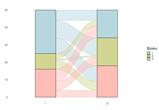
Figure 4: Alluvial plot for the membership of the nodes (different colors) in Layer 2 after 15 periods (horizontal axis) in the unidirectional causality setting (Example 1).

In the DSBMM, time is not only a dimension to measure the evolution of overlap between layers’ membership structure, but also it allows to evaluate the predictive power between membership structures. The structure in Layer 3 at $t=1$ not only overlaps with the structure of Layer 2 at the end of the time horizon, which introduces the idea of predictability, Layer 3’s membership structure has predictive power over Layer 2 structure fundamental in the notion of the Granger–causality concept [33]. At the same time, in the case of Layer 1, there is no pattern in the membership structure, which implies no causality.

Example 2.

The causality is bidirectional between Layer 2 and 3 and the main entries of its transition matrix is presented in Table 1. The matrix in each super–row and super–column refers to the transition matrix of Layer 2 (3). Similar to Figure 2, the Layer 2 probabilities (self–transition and between states) of matching states are higher and they do not depend on Layer 1, that is there is no variation between super–columns. However, unlike Figure 3 the transition probabilities of Layer 3 does depend on Layer 2, implying that there is Granger–block causality in both directions. Again, the Layer 1 does not play a role in changing the entries.

Table 1: Transition matrices in the bidirectional causality setting (Example 2). Each entry refers to the conditional transition probability in Layer 2 (3) given the membership in Layer 3 (2) (super–rows) and Layer 1 (super–columns).

		Layer 1
	Block	1	2
	1	$\begin{bmatrix}0.95&0.025&0.025\\ 0.34&0.65&0.01\\ 0.34&0.01&0.65\\ \end{bmatrix}$	$\begin{bmatrix}0.95&0.025&0.025\\ 0.34&0.65&0.01\\ 0.34&0.01&0.65\\ \end{bmatrix}$
Layer 3 (2)	2	$\begin{bmatrix}0.65&0.34&0.01\\ 0.025&0.95&0.025\\ 0.01&0.34&0.65\\ \end{bmatrix}$	$\begin{bmatrix}0.65&0.34&0.01\\ 0.025&0.95&0.025\\ 0.01&0.34&0.65\\ \end{bmatrix}$
	3	$\begin{bmatrix}0.65&0.01&0.34\\ 0.01&0.65&0.34\\ 0.025&0.025&0.95\\ \end{bmatrix}$	$\begin{bmatrix}0.65&0.01&0.34\\ 0.01&0.65&0.34\\ 0.025&0.025&0.95\\ \end{bmatrix}$

The dynamic of the membership for Example 2 is showed in appendix, in Figure D.12 with the same four dimensions of Figure D.11. Despite the fact that there is an overlap between the membership structure of Layer 3 and 2 at $t=15$, they are not similar to the one of Layer 3 at $t=1$, essentially ruling out unidirectional causality.

The DSBMM can include other cases or more complex context, such as overlap of only some communities, a decoupling effect of a Layer membership structure on others. Moreover, the multinomial saturated model in (5) cover higher order effects. For instance, Layer 1 membership structure can cause clustering overlap with Layer 2 coinciding with a decoupling effect on Layer 3.

3 Bayesian Inference

3.1 Prior specification

Given the presence of latent variables in the DSBMM, the observed likelihood is not tractable. Moreover, the specification (5) introduces all possible interaction effects between layers, causing an over–parameterization issue. A Bayesian approach addresses these issues and provides uncertainty measures of the latent variables and the parameters such as credible intervals [84]. The prior distributions used for the connectivity parameters and the initial partition of the nodes are described in Table 2. These priors are assumed to be independent and are commonly used in the SBM literature given its convenience as conditional conjugate [84, 79, 56]. It should be noticed that all parameters are scalar, but $\alpha^{(\ell)}$ and $\beta^{(\ell)}_{qr}$, the size of this latter depending on the number of covariates included.

Table 2: Prior distributions for connectivity parameters and initial node partitions

Prior distribution	Family
$\beta^{(\ell)}_{qr}\sim\operatorname{N}\left(\underline{\beta}^{(\ell)}_{qr},\underline{\Sigma}^{(\ell)}_{qr}\right)$	Normal
$\sigma_{qr}^{(\ell)2}\sim\operatorname{IG}\left(\underline{d}^{(\ell)}_{qr}/2,\underline{e}^{(\ell)}_{qr}/2\right)$	Inverse–gamma
$\nu^{(\ell)}_{qr}\sim\operatorname{Beta}\left(\underline{b}^{(\ell)}_{qr},\underline{c}^{(\ell)}_{qr}\right)$	Beta
$\alpha^{(\ell)}\sim\operatorname{Dir}\left(\underline{\alpha}^{(\ell)}\right)$	Dirichlet

Regarding the transition parameters of a Markov chain, the standard choice is a Dirichlet prior, but in our DSBMM, the multinomial representation of the HMC dependence call for the use of a conjugate informative prior: $\kappa_{q}^{(\ell)}\sim\operatorname{N}\left(\underline{\kappa}_{q}^{(\ell)},\underline{K}_{q}^{(\ell)}\right)$, with $\underline{K}_{q}^{(\ell)}=\zeta_{0}^{(l)2}{\bf I}_{p+1},\ \zeta_{0}^{(l)2}\in\mathbb{R}^{+}$, where ${\bf I}_{p+1}$ is a $p+1$ identity matrix and $\zeta_{0}^{(l)2}\in\mathbb{R}^{+}$ and $\underline{\kappa}_{q}^{(\ell)}\in\mathbb{R}^{p+1}$ are hyper–parameters [38, 32, 17]. The normal prior induces a ridge shrinkage pushing the estimates of the transitions probabilities away from zero and one, which is particularly useful for the entries of the transition matrix with few to none observations. However, this prior choice may still be unsatisfactory because it does not cope with the over–parameterization resulting from the inclusion of all layers and order effects in (5).

Since the main interest of DSBMM is to select the layers that have a significant impact on a specific transition matrix and not to select individual variables, applying a global shrinkage or a global variable selection method would not be coherent and it would omit an important information in considering the correlation between covariates—variable grouping.

We follow a Bayesian group–LASSO [72], through a Multi–Laplacian prior, which is equivalent to the flexible penalty used by [85] in the context of Poisson models for multidimensional contingency tables. The Multi–Laplacian prior can be interpreted as a continuous scale mixture of Normal distributions, as in [68]. The mixing distribution is a Gamma distribution, $\operatorname{G}(a,b)$ with shape parameter $a$ and scale parameter $b$. Thus, the Multi–Laplacian prior on the transition parameters has the following representation:

$$\qquad\qquad\qquad\qquad\qquad\kappa_{q}^{(\ell)}\sim\operatorname{N}\left(\underline{\kappa}_{q}^{(\ell)},\underline{K}_{q}^{(\ell)}\right)$$ (7)

$$\underline{K}_{q}^{(\ell)} =\operatorname{diag}\left(\zeta_{0}^{(l)2},\zeta_{q1}^{(l)2}\mathbf{1}_{s(1)}^{\prime},\ldots,\zeta_{0}^{(l)2}\mathbf{1}_{s(\ell)}^{\prime},\ldots,\zeta_{q\mathcal{U}}^{(l)2}\mathbf{1}_{s(\mathcal{U})}^{\prime},\ldots,\zeta_{q1\ldots L}^{(l)2}\mathbf{1}_{s(1\ldots L)}^{\prime}\right)$$

$$\qquad\qquad\qquad\qquad\zeta_{q\mathcal{U}}^{(l)2}|\rho^{(\ell)}\sim\operatorname{G}\left(\frac{s(\mathcal{U})+1}{2},\frac{2}{\gamma^{(\ell)}_{\mathcal{U}}}\right)$$

$$\qquad\qquad\qquad\qquad\qquad\rho^{(l)}\sim\operatorname{G}\left(\iota^{(l)}_{1},\iota^{(l)}_{2}\right)$$

where $2/\gamma^{(l)}_{\mathcal{U}}=2/\rho^{(l)}s(\mathcal{U})$ and $\iota^{(l)}_{2}$ are scale parameters, $s(\mathcal{U})$ is the number of covariates in the set of regressors $\mathcal{U}$. In this hierarchical structure, the prior variance $\underline{K}^{(\ell)}$ is not homoscedastic anymore, its diagonal elements are groupwise sampled from a Gamma distribution conditionally on $\rho^{(l)}$. The variable selection can be sensitive to the choice of $\rho^{(l)}$, because this latter has a direct relationship with the equivalent fixed parameter of the LASSO regression, $c$. Thus, a gamma prior is used for $\rho^{(l)}$ with hyperparameters $\iota^{(l)}_{1}$ and $\iota^{(l)}_{2}$. The penalization in (7) has a twofold effect, given that the set of covariates $\mathcal{U}$ in (5) corresponds to the interaction of different layers and orders, the $l_{1}$–penalty selects the most relevant orders and layers and within each of these relevant sets the $l_{2}$–penalty shrinks the parameters of highly correlated variables and those with few to no cases.

Comparing (7) with the original proposal by [72], two changes are introduced. First, contrary to a Poisson model for contingency tables, a multinomial logit implies $Q^{(\ell)}-1$ regressions, all of them sharing the same parameter $\rho^{(\ell)}$, in this way variable selection applies even across equations. This cross–equation information improves the estimation of $\rho^{(\ell)}$ by jointly contrasting more groups of variables. Second, not only the intercept of each of the $Q^{(\ell)}-1$ regression is excluded from the Multi–Laplacian prior, but also the main effects of the own layer in order to capture the HMC persistence. As a consequence, the variable selection do not apply to the intercept and the own lagged membership parameters, $Z^{(\ell)}_{it-1}$.

3.2 Posterior approximation

In order to estimate DSBMM, we propose a full Gibbs sampling approximation of the posterior distribution. Using (2), the complete likelihood can be expressed as

$$\begin{split}L(Y,Z,D|X,\vartheta)=\prod_{\ell=1}^{L}&\Bigg{(}\prod_{t=1}^{T}\left(\prod_{i\neq j}^{N}\left((1-D^{(\ell)}_{ijt})\delta(Y^{(\ell)}_{ijt})+D^{(\ell)}_{ijt}f^{(\ell)}\left(Y^{(\ell)}_{ijt}|\theta^{(\ell)}_{Z^{(\ell)}_{it}Z^{(\ell)}_{jt}}\right)\right)\right.\Bigg{.}\\ &\Bigg{.}\left.\left(\nu^{(\ell)}_{Z^{(\ell)}_{it}Z^{(\ell)}_{jt}}\right)^{D^{(\ell)}_{ijt}}(1-\nu^{(\ell)}_{Z^{(\ell)}_{it}Z^{(\ell)}_{jt}})^{1-D^{(\ell)}_{ijt}}\right)\Bigg{)}\left(\prod_{t=2}^{T}\prod_{i=1}^{N}\mathbb{P}(Z_{it}|Z_{it-1})\mathbb{P}(Z_{i1}|\alpha)\right)\end{split}$$ (8)

where it can be noticed that conditioning on $X$, the time and layer dependence is entirely driven by the HMCs. Additionally, consistently with the simulations in Section 2.3 and taking into account the literature on trade flows, we assume $f^{(\ell)}\left(y|\theta^{(\ell)}_{qr},X^{(\ell)}_{ijt}\right)$ is a log–normal distribution $\operatorname{LN}\left(\beta^{(\ell)}_{qr},\sigma^{(\ell)2}_{qr}\right)$. Nevertheless, our modeling framework is general and can be easily modify to account for other distribution assumptions. For example a zero–truncated Poisson family for count data applications [62, e.g., see]. Using the prior distributions presented in Section 3.1, the full conditional posterior distributions for the connectivity parameters, membership and initial proportions are derived in Appendix B with the details of the Gibbs sampler.

One of the main features of the DSBMM is its multinomial representation of the HMC dependence, but there is no conditional conjugate prior and the use of the standard Metropolis–Hasting algorithm presents the issue of tuning the parameters and can be inefficient. Following [32], we apply data augmentation to avoid Metropolis–Hastings steps. We extend the Pólya gamma representation proposed by [41] and [71] combining the data augmentation of the multinomial logit with the Multi–Laplacian prior expressed as a Normal mixture. Hence, the full conditional posterior of $\kappa_{q}^{(\ell)}$ can be rewritten as

$$h(\kappa_{q}^{(\ell)} |Z)\propto\int_{\mathbb{R}^{N(T-1)}}\underbrace{\pi\left(\kappa_{q}^{(\ell)}\right)\prod_{t=2}^{T}\prod_{i=1}^{N}\mathbb{I}_{\mathbb{R}^{+}}\left(\omega^{(\ell)}_{it,q}\right)\exp\left(\xi^{(\ell)}_{it,q}\eta^{(\ell)}_{it-1,q}-\omega^{(\ell)}_{it,q}\left(\eta^{(\ell)}_{it-1,q}\right)^{2}/2\right)h(\omega^{(\ell)}_{it,q})}_{h(\kappa_{q}^{(\ell)},\omega^{(\ell)}_{1:N1:T,q}|Z)}d\omega^{(\ell)}_{it,q}$$ (9)

where $\eta^{(\ell)}_{it-1,q}=\widetilde{W}_{it-1}\kappa_{q}^{(\ell)}-C^{(\ell)}_{it-1,q}$, $C^{(\ell)}_{it-1,q}=\log\left(\sum_{k\neq q}^{Q^{(\ell)}}\exp\left(\widetilde{W}_{it-1}^{(\ell)}\kappa_{k}^{(\ell)}\right)\right)$, $\xi^{(\ell)}_{it,q}=W^{(\ell)}_{it,q}-1/2$ and $\omega^{(\ell)}_{it,q}$ are auxiliary variables following a Pólya Gamma distribution, i.e. $\omega^{(\ell)}_{it,q}\sim\operatorname{PG}\left(1,0\right)$. Based on $h(\kappa_{q}^{(\ell)},\omega^{(\ell)}_{1:N2:T,q}|Z)$ in (9), let $\tilde{\xi}^{(\ell)}_{q}=\left(\xi^{(\ell)}_{12,q}/\omega^{(\ell)}_{12,q},\ldots,\xi^{(\ell)}_{NT,q}/\omega^{(\ell)}_{NT,q}\right)^{\prime}$ and $\eta^{(\ell)}_{q}=\left(\eta^{(\ell)}_{11,q},\ldots,\eta^{(\ell)}_{NT-1,q}\right)^{\prime}$ , then

$$h(\kappa_{q}^{(\ell)}|Z,\omega^{(\ell)}_{1:N1:T,q})\propto\pi\left(\kappa_{q}^{(\ell)}\right)\exp\left(-\frac{1}{2}\left(\tilde{\xi}^{(\ell)}_{q}-\eta^{(\ell)}_{q}\right)^{\prime}\Omega_{q}^{(\ell)}\left(\tilde{\xi}^{(\ell)}_{q}-\eta^{(\ell)}_{q}\right)\right)$$ (10)

where $\Omega_{q}^{(\ell)}=\operatorname{diag}\left(\omega^{(\ell)}_{12,q},\dots,\omega^{(\ell)}_{NT,q}\right)$ and $\xi_{q}^{(\ell)}=\left(\xi_{11,q}^{(\ell)},\dots,\xi_{N(T-1),q}^{(\ell)}\right)^{\prime}$. The full conditional distributions for $\kappa_{q}^{(\ell)}$ and $\omega^{(\ell)}_{it}$ are:

$$\kappa_{q}^{(\ell)}\left|Z,\omega^{(\ell)}_{1:N1:T,q}\right.\sim\operatorname{N}\left(\overline{\kappa}_{q}^{(\ell)},\overline{K}_{q}^{(\ell)}\right)$$ (11)

$$\omega^{(\ell)}_{it}\left|Z,\kappa_{q}^{(\ell)}\right.\sim\operatorname{PG}\left(1,\eta^{(\ell)}_{it-1,q}\right),$$ (12)

where

$$\overline{\kappa}_{q}^{(\ell)} = \overline{K}_{q}^{(\ell)}\left(\widetilde{W}^{\prime}\underbrace{\Omega_{q}^{(\ell)}\tilde{\xi}_{q}^{(\ell)}}_{\xi_{q}^{(\ell)}}+\widetilde{W}^{\prime}\Omega_{q}^{(\ell)}C_{q}^{(\ell)}+\left(\underline{K}_{q}^{(\ell)}\right)^{-1}\underline{\kappa}_{q}^{(\ell)}\right)$$ (13)

$$\overline{K}_{q}^{(\ell)} = \left(\widetilde{W}^{\prime}\Omega_{q}^{(\ell)}\widetilde{W}+\left(\underline{K}_{q}^{(\ell)}\right)^{-1}\right)^{-1},$$ (14)

The Pólya-Gamma representation has the compact expression

$$h(\kappa^{(\ell)}|Z,\omega^{(\ell)}_{1:N1:T})\propto\pi\left(\kappa^{(\ell)}\right)\exp\left(-\frac{1}{2}\left(\tilde{\xi}^{(\ell)}-\eta^{(\ell)}\right)^{\prime}\Omega^{(\ell)}\left(\tilde{\xi}^{(\ell)}-\eta^{(\ell)}\right)\right)$$ (15)

$$\kappa^{(\ell)}\left|Z,\omega^{(\ell)}_{1:N1:T,q}\right.\sim\operatorname{N}\left(\overline{\kappa}^{(\ell)},\overline{K}^{(\ell)}\right)$$ (16)

$$\overline{\kappa}^{(\ell)} =\overline{K}^{(\ell)}\left(({\bf I}_{Q^{(\ell)}-1}\otimes\widetilde{W})^{\prime}\xi^{(\ell)}+({\bf I}_{Q^{(\ell)}-1}\otimes\widetilde{W})^{\prime}\Omega^{(\ell)}C^{(\ell)}+\left(\underline{K}^{(\ell)}\right)^{-1}\underline{\kappa}^{(\ell)}\right)$$

$$\overline{K}^{(\ell)} =\left(({\bf I}_{Q^{(\ell)}-1}\otimes\widetilde{W})^{\prime}\Omega^{(\ell)}({\bf I}_{Q^{(\ell)}-1}\otimes\widetilde{W})+\left(\underline{K}^{(\ell)}\right)^{-1}\right)^{-1}$$

The full conditional of the group LASSO penalty hierarchical levels in (7) is given by

$$\zeta_{q\mathcal{U}}^{(l)2}\left|\kappa_{q}^{(\ell)},\rho^{(\ell)}\right.\sim\operatorname{GIG}\left(1/2,\gamma^{(\ell)}_{\mathcal{U}},||\kappa^{(\ell)}_{\mathcal{U},q}-\underline{\kappa}^{(\ell)}_{\mathcal{U},q}||^{2}_{2}\right)$$ (17)

$$\rho^{(l)}\left|\zeta_{q\mathcal{U}}^{(l)2}\right.\sim\operatorname{G}\left(\iota^{(l)}_{1}+\frac{(Q^{(\ell)}-1)(p-Q^{(\ell)}+1)+(2^{L}-2)(Q^{(\ell)}-1)}{2},\left(1/\iota^{(l)}_{2}+\frac{\sum_{q=1}^{Q^{(\ell)}-1}\sum_{\mathcal{U}}\zeta^{(l)2}_{q\mathcal{U}}s(\mathcal{U})}{2}\right)^{-1}\right),$$ (18)

where $\operatorname{GIG}$ denotes the Generalized Inverse Gaussian distribution [72].

In Figure 5, the DSBMM is summarized in a DAG (only for a layer $\ell$ for the sake of simplicity), excluding from the figure the hyperparameter of the prior distribution of the connectivity parameters and the initial partition of the nodes $\alpha^{(\ell)}$. In contrast to a DSBM, it includes the membership of the node in the other layers influencing the transition probability through the multinomial specification. In addition, the Multi–Laplacian prior selects the most relevant order and interactions of $\kappa^{(\ell)}$ and its Lagrange parameter is implicitly included in the inference procedure through $\rho^{(\ell)}$ whose prior information is captured by the hyperparameters $\iota^{(\ell)}_{1}$ and $\iota^{(\ell)}_{2}$ of a gamma distribution.

The last piece of the Gibbs sampler has to do with the allocation variables $Z^{(\ell)}_{i}$ sampling. Following [35] and [52], $Z^{(\ell)}_{i}$ are sampled using forward–filter–backward sampling (FFBS) algorithm using

$$\text{Prediction Probability}:\mathbb{P}\left(Z^{(\ell)}_{it}=q|Z^{{}^{(-\ell)}}_{i,1:t-1},Z^{{}^{(\ell)}}_{-i,1:t-1},\psi^{(\ell)}_{t-1}\right)$$ (19)

$$\text{Filtered Probability}:\mathbb{P}\left(Z^{(\ell)}_{it}=q|Z^{{}^{(-\ell)}}_{i,1:t},Z^{{}^{(\ell)}}_{-i,1:t},\psi^{(\ell)}_{t}\right)$$

$$\text{Smoothed Probability}:\mathbb{P}\left(Z^{(\ell)}_{i,1:T}|Z^{(-\ell)}_{i,1:T},Z^{(\ell)}_{-i,1:T},\psi^{(\ell)}_{T}\right),$$

where $\psi^{(\ell)}_{t}=[Y^{(\ell)}_{1:t},D^{(\ell)}_{1:t},X^{(\ell)}_{1:t}]$. The details of the each probability in (19) are presented in Appendix B. As discussed by [31, 46], given that under some mild conditions DSBM is identified up to label switching, these label changes may take place between Gibbs iterations. Some solutions to this issue lie on prior identification constraints or on the use of a random permutation sampler which allows to explore all the parameter space and then each iteration is classified across the different possible permutation in a post–Gibbs process [[, e.g.]]kaufmann2015k. Although either of these methods can be easily integrated into our Gibbs sampler, we do not report any problem in our simulations and application discussed below, in line with the simulation results in [84, 62] .

Figure 5: Directed Acyclic Graph of the DSBMM for layer $\ell$. Observed variables (gray circles), parameters and latent variables (white circles) and conditional dependence between them (arrows).

3.3 Synthetic data

We study the effectiveness of the model and the efficiency of the Gibbs sampler under different prior distributions for the transition parameters. We compare the accuracy in terms of causality detection of the DSBMM with a standard panel linear model used in the literature to infer Granger–causality. For each of model setting discussed in Section 2.3 and different sample size scenarios, 48 data sets are generated. Specifically, no causality, unidirectional or bidirectional examples are simulated alternatively with $N=50$ and $T=15$ (Reference sample size scenario), $N=100$ and $T=15$ (Larger N scenario) and $N=50$ and $T=30$ (Larger T scenario). The number of iterations used in each synthetic dataset is 2000 after convergence. The initialization of the Gibbs sampler requires an educated guess of $Z$, which is obtained by applying a DSBM individually on each layer, which in turn start with a time–invariant membership provided by the k–means algorithm on $D^{(\ell)}$ as suggested by [62].

The specific criteria used for membership accuracy is the Adjusted Rand Index (ARI), which is a chance adjusted measure of the proportion of pairs of nodes that are correctly classified in the same block or correctly classified in different blocks [44]. This index is applied globally to all $\mathcal{T}$ as suggested by [62]. A global ARI of 1 means that the Maximum a posteriori estimation (MAP) of $Z^{(\ell)}$ and the true latent memberships are the same up to label switching, otherwise the lower the ARI, the less identical are the two cluster structures and in case of a negative value, it would be equivalent to a worse performance than choosing the estimated membership at random.

Regarding the point estimate of the parameters, we rely on the Mean Square Error (MSE),

$$\operatorname{MSE}(\lambda^{(\ell)})=\frac{1}{Q^{(\ell)2}}\sum_{q,r\in\mathcal{Q}^{(\ell)2}}(\widehat{\lambda}_{qr}^{(\ell)}-\lambda_{qr}^{(\ell)})^{2}$$

where $\widehat{\lambda}_{qr}^{(\ell)}$ refers to posterior median and $\lambda_{qr}^{(\ell)}$ the true value, and the mean of $Q^{(\ell)2}$ elements is replaced by the mean of the $Q^{(\ell)}(Q^{(\ell)}+1)/2$ elements if the network is undirected.

Taking into account the importance of $\kappa^{(\ell)}$, another measure is added in the analysis, the Credible Interval Coverage (CIC), defined as,

$$\operatorname{CIC}(\kappa^{(\ell)})=\frac{1}{(Q^{(\ell)}-1)p}\sum_{q=1}^{Q^{(\ell)}-1}\sum_{\mathcal{U}\in 2^{\mathcal{L}}}\sum_{w=1}^{s(\mathcal{U})}\mathbb{I}_{\widehat{\mathcal{C}}^{(\ell)}_{\mathcal{U},q,w}}\left(\kappa_{\mathcal{U},q,w}^{(\ell)}\right),$$

where $\widehat{\mathcal{C}}^{(\ell)}_{\mathcal{U},q,w}$ is the range of values included in the 95% equal–tailed estimated credible interval for the parameter $\kappa_{\mathcal{U},q,w}^{(\ell)}$.

More importantly, the Granger–block causality is tested through the credible intervals, the layer $\mathfrak{m}$ is Granger–block causing layer $\ell$ if $\operatorname{GBC}(\mathfrak{m},\ell)=1$ and $\operatorname{GBC}(\mathfrak{m},\ell)=0$ otherwise, where

$$\operatorname{GBC}(\mathfrak{m},\ell)=\max_{\mathcal{U}|\mathfrak{m}\in\mathcal{U},q,w}\{1-\mathbb{I}_{\widehat{\mathcal{C}}^{(\ell)}_{\mathcal{U},q,w}}(0)\},$$

although, a more general approach to hypothesis testing can be used such as the Region of practical equivalence (ROPE) or other methods based on model comparison, e.g. Bayes factor [55, 74].

The prior hyperparameter values are given in Table 3. Specifically, the normal and gamma prior used for the connectivity parameters have a relatively large variance with respect to the observed datasets (for the true parameters see Appendix A). For the transition parameters in the multinomial Bayesian regression, in general the prior mean is zero and its variance comes from the Multi–Laplacian prior that induces a variable selection process, but some elements of $\kappa^{(\ell)}$ are excluded from this selection process. In light of the expected membership persistence in time and to avoid an undesired bias on variables that a priori are more relevant than the rest of regressors, all intercepts of (5) and $\kappa_{\ell,q,q}^{(\ell)}$, corresponding to main effects of the own layer, are not subject to the Multi–Laplacian prior, they have a fixed prior variance $\zeta_{0}^{(l)2}$, i.e. $\kappa_{0,q}^{(\ell)}\sim\operatorname{N}(-1,10)$ and $\kappa_{\ell,q,q}^{(\ell)}\sim\operatorname{N}(1,10)$, while $\kappa_{\ell,q,w}^{(\ell)}\sim\operatorname{N}(0,10),\ w\neq q$.

Finally, to set the hyperparameters $\iota_{1}^{(\ell)}$ and $\iota_{1}^{(\ell)}$, it should be kept in mind that $\rho^{(\ell)}$ is inversely related with the scale prior of $\zeta_{q\mathcal{U}}^{(l)2}$, hence large values of $\rho^{(\ell)}$ are associated with low prior variance on $\zeta_{q\mathcal{U}}^{(l)2}$ which may cause some bias and would not fully explore the parameter space. Therefore, $\iota_{1}^{(\ell)}$ and $\iota_{1}^{(\ell)}$ should result in a low prior mean and variance [68, see], .

Table 3: Prior Hyperparameters

Hyperparameter	Value	Hyperparameter	Value
$\underline{\beta}_{qr}^{(\ell)}$	${\bf 0}$	$\underline{\Sigma}^{(\ell)}_{qr}$	${\bf I}$
$\underline{d}_{qr}^{(\ell)}$	10	$\underline{e}_{qr}^{(\ell)}$	1
$\underline{b}_{qr}^{(\ell)}$	1	$\underline{c}_{qr}^{(\ell)}$	1
$\iota_{1}^{(\ell)}$	1	$\iota_{2}^{(\ell)}$	0.6
$\underline{\alpha}^{(\ell)}$	${\bf 1}_{Q^{(\ell)}}$	$\underline{\kappa}_{0,q}^{(\ell)}$	-1
$\underline{\kappa}_{\ell,q,q}^{(\ell)}$	1	$\zeta_{0}^{(l)2}$	10
$\underline{\kappa}_{\mathcal{U},q,w}^{(\ell)},\ \{\mathcal{U},q,w\}\neq\{\ell,q,q\}$	0

The results of the Gibbs sampler on the 48 datasets are presented in the box–plots in Figure 6 and 7 under different prior assumptions. Despite some outliers, generally the DSBMM is able to recover the correct classification of nodes in all layers and under different sample size scenarios and cases. Moreover, in terms of connectivity parameters, the MSE is kept close to zero, that is the difference between posterior medians and the true parameters is negligible under normal prior and LASSO prior.

Nevertheless, the same cannot be said with the MSE and CIC of the transition parameters $\kappa^{(\ell)}$. In particular, under a Bayesian group LASSO prior for $\kappa^{(\ell)}$, the MSE is lower, less disperse and with fewer outliers, but in terms of coverage (CIC) the Normal prior performs slightly better. This reflects the trade–off between variance and unbiasedness in the over–parametrized multinomial model. Under a Normal prior, whose implicit penalty only shrinks the estimates, the credible intervals are larger containing the true parameters in most of the cases, while under a Multi–Laplacian prior, that allows for group penalization and variable selection, the lower MSE suggests a better balance between bias and variance. Still, under both priors, the Example 2 of bidirectional Granger–block causality is harder to estimate, but close to the results found in the multidimensional sparse contingency table literature [22, e.g.,].

Since the main focus is on causality detection, Table 4 gives information on the proportion of datasets where the Gibbs sampler correctly inferred the full causality structure. It can be seen that Bayesian Lasso prior clearly performs better than the Normal prior (see Figure 6 and 7). Under a Normal prior the DSBMM tends to have a larger type I error. Basically, the highly parameterized multinomial model affects the credible intervals under the standard Normal prior, and the Bayesian LASSO overcome this difficulty inducing a variable selection process and grouping the variables according to our main interest—layer dependence and order. It is important to notice that the performance of the Bayesian group LASSO is affected by the sample size and cases, specially for larger $T$ and for the bidirectional case, still the proportions of causality structure correctly identified are high and the individual GBC for each pair of layers performs well (see Figure D.15 and D.16).

The concept of Granger causality is intrinsically related to the standard BVAR and panel BVAR models and they have been extensively used in empirical work [[, e.g., see]]canova2013panel,sims1980macroeconomics,koop2013forecasting,dieppe2016bear. However, we find evidence that BVAR models have difficulties in detecting the Granger–block causality generated by the DSBMM model. In this framework, it would be a short panel, where each layer represents a variable and the cross–sectional units correspond to the dyads of the network that are observed for $T$ periods. Three more sub–scenarios are added to the simulations: WNZ, where all layers are weighted and fully connected; WZ, layers are weighted, but not fully connected; and UW, which is the sub–scenario with one unweighted layer and two weighted one, non of them fully connected. This latter is the sub–scenario used in the previous DSBMM simulations and described in Appendix A.

The result of the comparison panel BVAR models and DSBMM are shown in Table C.6. It can be noticed that none of Panel BVAR model is able to detect the correct causality structure, but the pooled panel BVAR. However, this latter correctly inferred the causality structure under a specific scenario: if all layers are weighted, fully connected and the sample size is larger in $T$. When there is some sparsity in the layers, or if one of them is unweighted, or under smaller $T$, the proportion of datasets where the BVAR correctly inferred the full causality structure drops dramatically and far from the performance of DSBMM. Consequently, the BVAR framework generally do not capture the Granger–block causality, only under conditions that are not common in network data.

Table 4: Proportion of simulated data sets where the true causality structure is successfully retrieved by model setting, sample size and prior

Model setting	Sample size	Normal Prior	Bayesian Lasso
No causality	Reference	0.25	0.96
	Larger N	0.10	0.92
	Larger T	0.27	0.88
Unidirectional	Reference	0.52	0.96
	Larger N	0.46	0.92
	Larger T	0.46	0.83
Bidirectional	Reference	0.52	0.92
	Larger N	0.31	0.88
	Larger T	0.44	0.79

Note: Reference sample size is $N=50$ and $T=15$, Larger $N$ is $N=100$ and $T=15$ and Larger $T$ is $N=50$ and $T=30$. The number of datasets generated in each scenario is 48. In each dataset the number of iterations is 2000 and a burn–in of 1000.

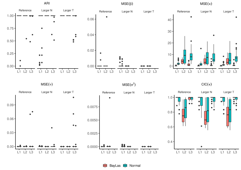
Figure 6: Performance in unidirectional causality setting (Example 1). Box-plots of global Adjusted Rand Index (ARI), Mean–Squared Error (MSE) of connectivity and transition parameters and credible intervals coverage (CIC) under Normal and Group–Lasso Prior assumption (colors) for the three layers (L1, L2 and L3) and various sample sizes (Reference, Larger N and Larger T).

Note: Reference sample size is $N=50$ and $T=15$, Larger $N$ is $N=100$ and $T=15$ and Larger $T$ is $N=50$ and $T=30$. The number of datasets generated in each scenario is 48. In each dataset the number of iterations is 2000 and a burn–in of 1000.

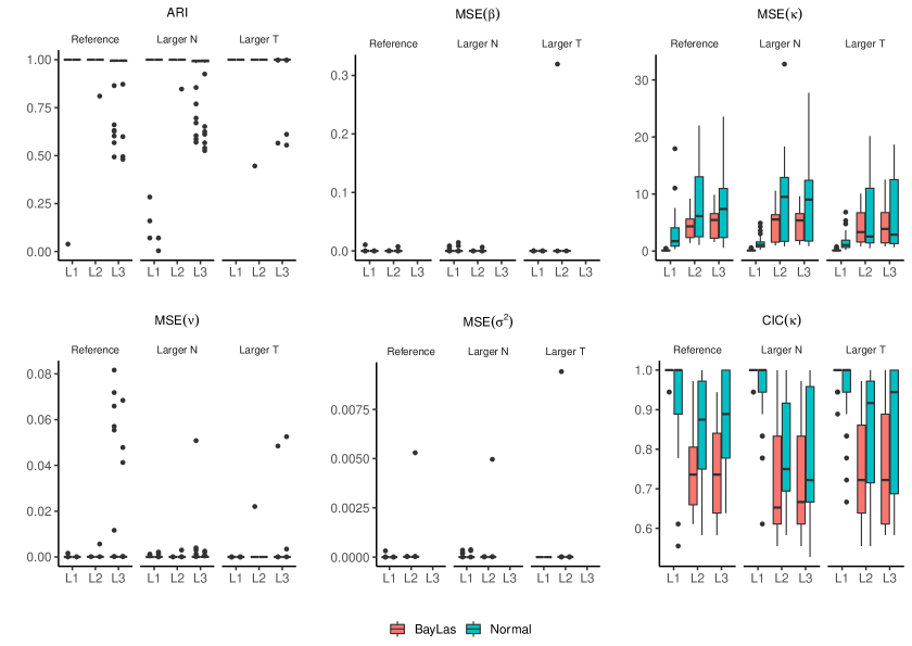
Figure 7: Performance in the bidirectional causality setting (Example 2). Box-plots of global Adjusted Rand Index (ARI), Mean–Squared Error (MSE) of connectivity and transition parameters and credible intervals coverage (CIC) under Normal and Group–Lasso Prior assumption (colors) for the three layers (L1, L2 and L3) and various sample sizes (Reference, Larger N and Larger T)

Note: Reference sample size is $N=50$ and $T=15$, Larger $N$ is $N=100$ and $T=15$ and Larger $T$ is $N=50$ and $T=30$. The number of datasets generated in each scenario is 48. In each dataset the number of iterations is 2000 and a burn–in of 1000.

4 The impact of FTAs on the trade network structure

We apply our DSBMM to international trade and show that it provides a general and unified framework merging two research lines: the Gravity model and the community detection literature, allowing study causality at a global level. Our model allows for new evidence in the trade literature within a coherent inference framework. Since the General Agreement of Tariffs and Trade, FTAs have been an important tool conceived as a means to increase trade flows among countries. We use the DSBMM to infer the causal relationship between FTAs and trade flows.

4.1 Gravity model, communities and the DSBMM

Empirical studies, starting by [80], have followed the Gravity equation to explain bilateral trade and infer the effect of trade policies. From the applied point of view, this equation proposes the economy size (e.g. GDP, population) and the frictions (e.g. physical distance,language similarity, colonial links) of the countries involved as the determinants of trade flows. Although this gravity framework started as an intuitive empirical regularity, a theoretical foundation is possible using a general equilibrium model in a static framework à la Heckscher–Ohlin with monopolistic competition [5, 48, see for example]. These models interpret trade flows beyond a dyad relationship and they bring attention to the structure of the trade network. In particular, in its reduced form, this family of models can be written as

$$\begin{cases}\log\left(Y^{(1)}_{ij}\right)=\beta^{(1)}_{0}+\beta^{(1)}_{1}GDP_{i}+\beta^{(1)}_{2}GDP_{j}+\beta^{(1)}_{3}t_{ij}+\beta^{(1)}_{4}\Upsilon_{j}+\beta^{(1)}_{5}\Pi_{i}+\varepsilon_{ij}\\ \left(\Pi_{i}\right)^{1-\varrho}=\sum_{j=1}^{N}\left(\frac{t_{ij}}{\Upsilon_{j}}\right)^{1-\varrho}\frac{GDP_{j}}{\sum_{k}^{N}GDP_{k}}\\ \left(\Upsilon_{j}\right)^{1-\varrho}=\sum_{i=1}^{N}\left(\frac{t_{ij}}{\Pi_{i}}\right)^{1-\varrho}\frac{GDP_{i}}{\sum_{k}^{N}GDP_{k}},\ \varrho>1\end{cases}$$ (20)

where trade $Y^{(1)}_{ij}$ increases with the node characteristics $GDP_{i}$ and $GDP_{j}$, i.e. $\beta_{1},\beta_{2}>0$, and the frictions $t_{ij}$ have a negative effect on trade, $\beta_{3}<0$. The barriers are partially observed, particularly for this application only the information on distance between countries ($dist_{ij}$) is available and all the rest of components are unobserved ($\tilde{t}_{ij}$) including differences in FTAs, technology and non–tariff barriers between countries, then $t_{ij}=\lambda dist_{ij}+\tilde{t}_{ij}$. The two fully unobserved elements $\Upsilon_{j}$ and $\Pi_{i}$ affecting the trade flow between $i$ and $j$, called inward and outward multiresistance respectively, encompass an aggregated measure of the barriers between all the pairs of nodes in the trade network. Under some circumstances, these multiresistance terms may not include information on all the network, but only on the barriers of the neighboring nodes of country $i$ and $j$, as in the Gravity model proposed by [59]. This latter model underlines the existence of two communities in the trade network: a core and a periphery, due to firms behavior that choose their export destinations based on a pecking order. Other authors suggests that firms choose new destinations that are similar to previous ones, given the high cost of adapting products to heterogeneous markets, which may implicitly produce blocks of countries. Based on these considerations, a block structure in the network of barriers $t_{ij}$ can be directly or indirectly creating communities on $Y^{(1)}_{ij}$, that is through $t_{ij}$, and also $\Upsilon_{j}$ and $\Pi_{i}$. For instance, this motivates the empirical works of [77], that study the overlap between FTAs and trade network from a dyad perspective in (20).

Since FTAs are part of the unobserved frictions $\tilde{t}_{ij}$, the DSBMM can be used to test if the community structure in the FTA network is Granger–causing the block membership in the trade network . However, this is not the only possible scenario because FTAs are not fully exogenous. As posed by [7]’s theoretical model the welfare expectations of consumers and firms may depend on the pre–policy levels of trade flows and acting on the likelihood of a FTA. Moreover, integration processes, domestic regulations and production fragmentation are inducing changes in both networks and may cause clustering patterns [61, 8, 10, 45, 15, e.g.]. Thus, it is not clear if FTAs and trade flows are unidirectional or bidirectional related in the Granger–block sense and the empirical evidence obtained from panel analysis and impact evaluation methods on FTAs effectiveness at a dyad level shows mixed evidence [7, for a review see].

The application of DSBMM to the trade and FTA network provide a unified framework of two stream of literature that have been developing separately: the Gravity model and FTA effectiveness and the works related to community detection. Compared to the literature on FTA effectiveness, a Granger–block causality approach is close to the spatial econometric techniques used to control for multiresistence terms or to measure the impact of the neighboring nodes’ characteristics on trade [15, 30, e.g.]. Nevertheless, DSBMM is conceptually different because the blocks that constitutes the various neighborhoods are not only unobservables, but dynamic, additionally it introduces parameter heterogeneity in the linear model (20) instead of a constant parameter capturing the effect of an spatial lag.

Regarding the literature on community detection in the trade and FTA network, it has followed algorithmic methods such as maximizing a modularity measure to identify groups of countries with dense subgraphs, as in [13, 14]. In this sense, DSBMM provides a statistical model and subsequently its inference includes a measure of uncertainty of the parameters, and the latent membership. It also allows for dynamic membership of nodes and covariates to control for node characteristics which is essential to link the community structure with the Gravity equation. Specifically, we suggest that detecting communities in the trade flows after controlling for the observed covariates in (20), focuses the attention on the blocks detection in the unobserved components, that is the multiresistence terms and the unobserved barriers to trade, resulting in a partial pooling of the linear model, i.e.

$$\log\left(Y^{(1)}_{ijt}\right)=\check{\beta}^{(1)}_{0qr}+\beta^{(1)}_{1}GDP_{it}+\beta^{(1)}_{2}GDP_{jt}+\beta^{(1)}_{3}\lambda dist_{ij}+\varepsilon_{ijt},$$

where $\check{\beta}^{(1)}_{0qr}=\beta_{0}+\beta_{3}\tilde{t}_{qr}+\beta_{4}\Upsilon_{r}+\beta_{5}\Pi_{q}$ and $q,r\in\mathcal{Q}^{(1)}$. Considering the information across time, the time index is added and the partial pooling applies in both dimensions: cross–sectional (dyad) and time. This can be generalized by allowing all parameters to be block dependent and by dropping the assumption of a fully connected trade network which yields a specification equivalent to (1). Then, the first layer of a multi–layer network with $L=2$ is

$$Y_{ijt}^{(1)}\left|X_{ijt},Z^{(1)}_{it}=q,Z^{(1)}_{jt}=r,\vartheta^{(1)}\right.\sim(1-\nu^{(1)}_{qr})\delta(y)+\nu^{(1)}_{qr}\operatorname{LN}\left(\left(\beta_{qr}^{(1)}\right)^{\prime}X_{ijt},\sigma^{2}_{qr}\right),\ q,r\in\mathcal{Q}^{(1)}$$ (21)

where $X_{ijt}=\left(GDP_{it},GDP_{jt},dist_{ij}\right)^{\prime}$ and $\beta_{qr}^{(1)}=\left(\check{\beta}^{(1)}_{0qr},\beta^{(1)}_{1qr},\beta^{(1)}_{2qr},\beta^{(1)}_{3qr}\lambda_{qr}\right)^{\prime}$. The second layer,

$$Y_{ijt}^{(2)}\left|Z^{(2)}_{it}=q,Z^{(2)}_{jt}=r,\vartheta^{(2)}\right.\sim\operatorname{Bern}\left(\nu^{(2)}_{qr}\right),q,r\in\mathcal{Q}^{(2)}.$$ (22)

corresponds to the unweighted and directed FTA network, and it has its own community structure. This specification (21) and (22) allows us to test if the community structure in the unobserved barriers and multiresistance terms is related to the block membership of the FTAs.

For example, if $Q^{(1)}=Q^{(2)}=2$, (5) becomes

$$\log\left(P^{(1)}_{it,1}C^{(1)}_{it}\right) =\kappa^{(1)}_{0,1}+\underbrace{\kappa^{(1)}_{\{1\},1,1}W^{(1)}_{it-1,1}+\kappa^{(1)}_{\{2\},1,1}W^{(2)}_{it-1,1}}_{\text{main effects}}+\underbrace{\kappa^{(1)}_{\{1,2\},1,1}W^{(1)}_{it-1,1}\cdot W^{(2)}_{it-1,1}}_{\text{first order effects}}$$ (23)

$$\log\left(P^{(2)}_{it,1}C^{(2)}_{it}\right) =\kappa^{(2)}_{0,1}+\underbrace{\kappa^{(2)}_{\{1\},1,1}W^{(1)}_{it-1,1}+\kappa^{(2)}_{\{2\},1,1}W^{(2)}_{it-1,1}}_{\text{main effects}}+\underbrace{\kappa^{(2)}_{\{1,2\},1,1}W^{(1)}_{it-1,1}\cdot W^{(2)}_{it-1,1}}_{\text{first order effects}},$$

and the Granger–block tests can be stated as: FTAs does not Granger–block cause unobserved barriers and multiresistence terms network, $H_{0}:\kappa^{(1)}_{\{2\},1,1}=\kappa^{(1)}_{\{1,2\},1,1}=0$; or, trade network does not Granger–block cause FTAs network on the effect of FTAs on trade, $H_{0}:\kappa^{(2)}_{\{1\},1,1}=\kappa^{(2)}_{\{1,2\},1,1}=0$.

4.2 Data description

The dataset used in this application includes 159 countries detailed in Table C.10, for the period 1995–2017. The trade network corresponds to the value of all goods imported (CIF) between pairs of countries collected by the International Monetary Fund (IMF) in U.S. dollars, which are transformed into constant terms by using the GDP PPP deflator from the same source with base year 2010, as in [39]. The information reported to the IMF is not always complete, either due to missing reporting countries (nodes) or specific flows (edges) at a period $t$. The IMF applies some imputation techniques that minimize the missing edges and approximate the information on the non–reporting countries, including mirror information (reported exports between pairs), total imports and exports of the reporter country among other adjustments aiming at consistency between monthly, quarterly and annual data. The IMF makes available the final outcome of this process indicating that any specific bilateral trade that is not included in the database can be considered as zero [25].

Regarding the FTAs, the network is constructed using the database on Economic Integration Agreements of the NSF–Kellogg Institute. The information provided on type of FTA is dichotomized to the existence or not of any trade agreement, from a non–reciprocal preferential trade arrangement (NR–PTA) to Economic Union (EUN). The former type of agreement makes the adjacency matrix of the FTAs not symmetric. This data is collected from various sources, such as the CIA World Factbook or the WTO database among others, if there is not information on any of the sources for a pair of countries, the database includes FTAs based on trade flows. For instance, if two countries have never traded and there is no international agreement among them in the databases reviewed, it is assumed that they have not signed a FTA. Although, these imputations covered 40% of the pairs between 1950–2012, the assumptions are reasonable and commonly accepted in the literature on FTA effectiveness [9, 27, e.g.]. Finally, the covariates used for the first layer are from the dynamic gravity dataset of the U.S. International Trade Commission (USITC), that collects GDPs in real terms from the World Development Indicators (WDI) and the distance ($dist_{ij}$) refer to the population weighted distance between each pair of countries [34].

A general description of the resulting multi–layer FTAs–Trade Flows is presented in Table 5 that confirms some of the stylized facts in the empirical analysis of international trade. Since the beginning of the period both networks are dense and without taking into consideration the direction of the edges there is only one components (WCC), that is there exists always a path to connect a pair of countries. If the direction is introduced (SCC) the FTA has more than one components due to the presence of regional agreements and the non–reciprocal agreements between developed and developing countries, which makes some nodes unilaterally unreachable, i.e. there exists a path from $i$ to $j$, but no vice–versa. Through time, the FTAs network converges to one component, as in the trade network from the beginning of the period, due to the higher edge density.

On the other hand, it can be seen that trade network is significantly more connected than the FTAs and in both of them the average degrees and density tends to increase through time, which can be a first indication of dependence. Consistently with this higher connectivity, the average path length for the unweighted layer has decreased, but it cannot be said the same of the weighted one, despite its general decline it experiences a reverse trend in the 2000s. In this sense. The number of triangles in the FTA and trade networks has steadily increased resulting in higher clustering coefficients. Moreover, the betweenness centrality is decreasing for both networks, which can be interpreted as a loss of influence of intermediary nodes given the presence of new one–step shortest paths and an average increase of the connectivity of the nodes.

Both layers share common trends in most of the indicators in Table 5. The joint changes in the connectivity features may suggest a significant impact of trade policies on the community structure of the unobserved factors of the trade network. In order to find evidence of this possibility within a DSBMM framework, there must be a community structure in the trade flows network even after controlling for GDP and distance, which to the best of our knowledge has not been directly tested in the literature. Moreover, the changes of this unobserved structure must be related to the changes in trade policy through their memberships dynamics.

Table 5: Connectivity in the Multiplex FTAs–Trade Flows

Year	$AD$	$AID$	$De$	$APL^{\dagger}$	$WCC^{\dagger}$	$SCC^{\dagger}$	$AClueCoe^{\dagger}$	$ABetCent^{\dagger}$
FTA Layer (unweighted and directed)
1995	51.69	25.84	0.16	2.68	1	31	0.36	153.75
2005	79.65	39.82	0.25	2.23	1	5	0.49	169.09
2015	97.38	48.69	0.31	1.88	1	1	0.53	139.03
Trade Flow Layer (weighted and directed)
1995	169.84	84.92	0.54	8777.24	1	1	0.94	749.3
2005	215.85	107.92	0.68	1341.3	1	1	0.96	658.98
2015	244.42	122.21	0.77	1854.54	1	1	0.97	648

Note: Average Degree ($AD$), Average In–Degree ($AID$), Density ($De$), Average Path Length ($APL$), Number of Weakly and Strongly Connected Components ($WCC$ and $SCC$), Average Clustering Coefficients ($ACluCoe$), Average Betweenness Centrality ($ABetCen$). The indicators with $\dagger$ accounts for the weights of the Trade Flows, otherwise only the $D^{(1)}$ is used.

4.3 Results

In order to apply the DSBMM to the FTAs–Trade flows multi–layer in (21) and (22), we assume that $Q^{(\ell)}$ is known. Based on [59], a core–periphery structure is a parsimonious representation of the trade flow network. Thus, it can be described by two communities: a core, that is a subset of highly connected nodes and a periphery, the rest of nodes that are more densely linked to the core than to the other nodes in the periphery. This can be interpreted using a pecking order scheme, firms in each country export following a destination list ordered according to market size and lower trade costs. Hence, countries with less productive firms (periphery) are only able to trade with the top of the list, while the countries with more productive firms (core) can trade with large and smaller markets and/or less and more costly destination. Regarding the FTAs layer, four communities are considered, and the results for another choice is summarized in Figure D.20.

Some alternatives to select the number of communities are to minimize the Deviance Information Criteria (DIC) proposed by [20] and computationally integrated to FFBS for HMC by [49], or to maximize the Integrated Classification Likelihood (ICL) criterion as in [62]. However, the performance of these criteria on a network data with high degree heterogeneity is not satisfactory neither theoretically nor in synthetic data [86, 83, 42]. Indeed, [42] proposes a corrected Bayesian Information Criterion (CBIC) in the static framework, since comparing different criteria applied to the trade network leads to significant variation in the number of communities suggested, between 1 to 10 blocks. Adapting DIC and ICL, used in [49] and [62] respectively, to the individual layers of the network data collected here, results in more than 11 communities in each of them. The same suggestion holds for the trade network even after controlling for the observed dyad and node heterogeneity $X_{ijt}$, which may reflect that the unweighted part $D_{ijt}$, also presents a high degree heterogeneity. In fact among the 11 communities, some of them are small groups potentially due to this diversity in node degree, which may influence DSBMM outcomes. Given the unsatisfactory performance of these criteria, $Q^{(\ell)}$ is kept known for the application here.

The results under $Q^{(1)}=2$ and $Q^{(2)}=4$ confirm a core–periphery structure in Layer 1. Community 1 corresponds to the core with almost a fully connected sub–graph in terms of intra–block edges (value of $\nu_{11}^{(1)}$ close to 0.98 in Figure 8) and is highly dense in the inter–block edges to community 2 (value of $\nu_{12}^{(1)}$ close to 0.84). The community 2 is the periphery, that is better connected to the core (value of $\nu_{21}^{(1)}$ close to 0.79) than to other nodes within its block (value of $\nu_{22}^{(1)}$ close to 0.36). Additionally, the highest variance in the flows is from or within the periphery (values of $\sigma_{21}^{(1)2}$ and $\sigma_{22}^{(1)2}$ close to 8.2 and 8.5), while the flows related to the core has lower variability. This results opposes to the existent model used in the literature that impose larger variance to larger trade flows [75]. In the second layer, the structure seems more complex, except for community 3, where intra–block connectivity $\nu_{qq}^{(\ell)}$ is higher than its inter-block counterpart, the other blocks have a non–assortative feature, that is community 1, 2 and 4 are highly connected to block 3 and less densely linked to the other communities. This configuration is compatible with a core–periphery graph, but with some particularities. The core is the community 3 that includes the countries with the highest centrality such as the U.S. and western Europe. The periphery are the rest of the blocks. For instance, the intra–edges of community 4 are almost as dense their in–degree from the core, which is the case of countries from eastern Africa (see Figure D.19). The block structure in the trade flows is coherent with the hypothesis of the picking order destination list. In particular, the most productive firms in the periphery (and in the core), which are those able to export, give priority to the destinations with large market size and lower trade costs (the core) [59]. However, it is not clear from this theory why the flows from the periphery to the core seems to be more unstable (higher variance), it could be due to supply factors such as productivity heterogeneity across countries in the periphery or demand factors from the core given that densely connected countries may have more alternative suppliers to consider.

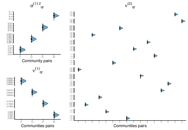
Figure 8: Empirical density of the posterior distribution of the variance of the trade network log–weights residuals ($\sigma_{qr}^{(1)2}$) and the sparsity parameters for the Trade and FTA network ($\nu_{qr}^{(1)}$ and $\nu_{qr}^{(2)}$ ) by block interactions (x–axis)

Note: Each distribution corresponds to a different block interactions $qr$, where the first number $q$ refers to the community of the exporter and the second number $r$ to the community of the importer (x–axis). Number of simulations: 30,000 and burn-in: 10,000. Thinning: 10.

Regarding the connectivity parameters in the Gravity equation, the results evidence significant differences between blocks which in turn reflect contrasting unobserved barriers and multiresistance terms. The intercept between core nodes show the highest barriers, while for the peripheral nodes this parameter it is even trade–enhancing. At the same time, this is compensated by a less negative distance parameter between the core countries and an almost twice negative effect within community 2. A similar pattern applies to the exporter and importer GDP elasticities, both are higher in the core. In the inter–block interaction, when the core (periphery) is the exporter trade flows are more (less) responsive to the GDP in contrast to its role as importer. Hence, the heterogeneity in the Gravity equation parameter are coherent with the differences in the connectivity parameters of the unweighted part of the trade network ($\nu^{(1)}$) and the international trade literature studying intensive and extensive margins [16, see for example]. The gaps in the distance parameter can be explained by the difference in technology and/or transportation costs. In the case of the GDP elasticities, the differences suggest the possibility of persistent trade deficits for the periphery, which is not fully accounted by standard trade theory that assume the elasticities should be close to one for all countries.

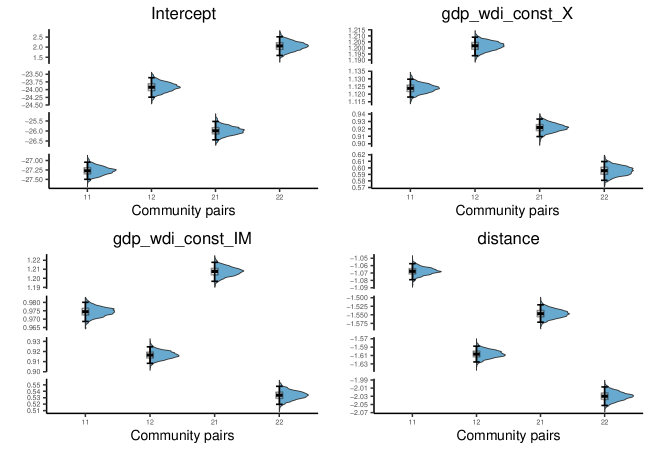
Figure 9: Empirical density of the posterior distribution of the Gravity equation parameters in the trade network by blocks interaction under $Q^{(1)}=2$ and $Q^{(2)}=4$

Note: Each distribution corresponds to a different block interactions $qr$, where the first number $q$ refers to the community of the exporter and the second number $r$ to the community of the importer (x–axis). Number of simulations: 30,000 and burn-in: 10,000. Thinning: 10.

This network structure is not static and countries may change of membership through time and inherits the corresponding set of connectivity parameter which to the extent of our review is not taken into account in standard partial or general equilibrium model used for ex-post and ex-ante trade policy evaluation [70, e.g.,]. In this sense, for the trade network 22.0% of countries change of membership at least one time between 1995–2017 mostly from periphery to core, while in the FTA layer all countries deviate from its initial community (see Figure D.17 and D.18). This new result complement the existent community detection studies on trade flows that deduce the increase in density of the network identifying the blocks at each point in time, but given its static approach it was not possible to recover specific node changes.

The block dynamic allows to test for Granger–block causality and check if the changes in the membership structure of the FTAs and in the unobserved components of the Trade network are related. In Figure 10, the membership dependence between the two layers of the multi–layer is summarized into four graphs, each of them associated with a vector $\kappa_{q}^{(\ell)}$. For instance, the first graph shows the transition probability of moving/stay in community 1 (core) of the trade network and it can be noticed that only its diagonal element are significant, i.e. $W^{(1)}_{it-1,1}$ and the intercept, which denotes persistence in membership. More importantly, this persistence is attenuated by the influence of the countries’membership in the FTA network, essentially a change of membership to the core in the FTA network induces a change in the trade network producing a decrease in the multiresistence terms and unobserved barriers. The three graphs left describing FTA network transition parameters indicate that the membership persistence is lower, compared to the Trade network, but it is not affected by the block structure of this latter. Therefore, there is evidence of unidirectional Granger–block causality from the FTA’s block structure to the Trade membership. See the Appendix for further results.

The unidirectional block–causality suggest that the FTA have effectively modified the trade flows network structure favoring the transition of countries from the periphery to the core and increasing the global trade integration. The unidirectional dependence also seems to support the FTA exogeneity at block level, despite that the existent literature show evidence of FTA endogeneity at dyad level. In other words, the current level of trade for a specific pair of countries also affects their probability of signing or not a FTA, but in general it is more difficult to argue the same for a set of countries in the same block considering that each of them follow their own trade policies. An exception would be the European Union, but most of their members were already in the core by 1995 and did not experienced membership changes. Still some countries are not part of the core of FTA network and are densely connected in the trade network (e.g. China and Costa Rica). This could be due to the type of exported products, technological particularities, the level of integration to the Global Value Chains (GVC), among other factors which can be easily included in the DSBMM as extra covariates or as extra layers (e.g. the global investment network). Moreover, the time varying membership captured by our DSBMM implies evidence of parameter heterogeneity in the Gravity equation, which is usually used by the trade literature to evaluate the impact of changes in tariffs. This heterogeneity is specially relevant in the evaluation of trade policies aiming at a structural change of the network beyond a specific dyad of countries in the same community, for example the theoretical scenarios of full autarky or in ambitious treaties such as the Transatlantic Trade and Investment Partnership (TTIP) or the Trans–Pacific Partnership (TPP), in these cases the counterfactual scenario may also imply different parameters.

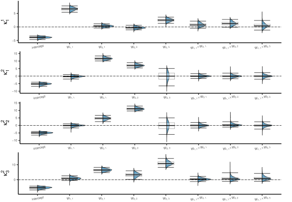
Figure 10: Empirical density of the posterior distribution of the transition probability parameters of the multinomial model for the Trade (Layer 1) and FTAs (Layer 2) network using as reference equation $Q^{(1)}=2$ and $Q^{(2)}=4$

Note: Number of simulations: 30,000 and burn-in: 10,000. Thinning:10.

5 Conclusion

This work has focused on extending the DSBM to a multi–layer setting with HMC dependence. This task is achieved assuming node membership is driven by a different HMC in each layer. The HMC dependence across layers is specified as a saturated multinomial logit model. The resulting model, DSBMM, allows to study the relationship between layers’ block structure and it provides a framework for a Granger–block causality test.

The dependence in transition probabilities is able to capture coupling trends between the membership structure of the layers, decoupling tendencies, or more complex relationships. Compared to the existent literature on multi–layer SBM that gives only a correlational measure between layers, the DSBMM not only gives information on the dependence in terms of sign and magnitude, but also on its direction.

For the estimation of the DSBMM, we propose a full Gibbs sampler accounting for (un)weighted and (un)directed layers with potential layer–specific covariates controlling for node and dyad heterogeneity that affect the weights of the networks or the sparsity. The main issue in the posterior approximation is the multinomial model of the transition matrices. Using a Pólya Gamma representation, it is possible to keep the full Gibbs sampler through the use of auxiliary variables $\omega^{(\ell)}_{it}$. In order to cope with the large number of transition parameters, we combine the Pólya Gamma representation with a Multi–Laplacian prior that gives rise to a process of variable selection that considers the group of variables based on order of interaction and layers. This prior induces a $l_{1}$–penalty between groups and $l_{2}$–penalty within each group, which accounts better for the correlation structure of the covariates of the multinomial representation, even across equations of the same layer.

Under DSBMM, different scenarios are generated, including no causality, unidirectional and bidirectional causality between layers, to evaluate the performance of the Gibbs sampler. The sampler is able to recover the membership in each layer and the connectivity parameters. The simulations evidence that the Multi–Laplacian prior performs better than a Normal prior for the transition parameters, $\kappa^{(\ell)}$, in terms of Granger–block causality detection. Comparing with BVAR models used to test for Granger causality, this latter are not able to identify the Granger–block relationship between layers, but only under the particular scenario where all layers are fully connected network and weighted, which although common in time series data it is not in dynamic network data, where the sparsity and unweighted relationships are more standard. Hence, DSBMM provides a better fitting than existing methods, especially when the nature of the variables are different, that is discrete, continuous or mixed random variables.

We exemplify the use of DSBMM in the context of international trade. To the best of our knowledge is a first effort to integrate these two streams of literature: community detection and Gravity models. Considering the data on Trade Flows and FTAs, a dynamic multi–layer of 159 countries and 23 years is constructed. The DSBMM detects a core–periphery structure in FTAs and in the trade network. Moreover, it evidence a dyad and time heterogenity of the Gravity equation parameters, which is not covered by the standard theoretical models and may affect the existing methods for FTA evaluations. Finally, we find new evidence of unidirectional Granger–block causality from the FTAs to the unobserved barriers membership structure, which contribute to the debate on FTAs effectiveness beyond the dyad level. Some extensions to consider in the DSBMM are a criterion to choose the number of communities in each layer and the introduction of other definitions of causality using a counterfactual framework.

Appendix A Connectivity parameters

The connectivity parameters and initial partition used in the data generated process of all examples are:

$$\alpha^{(1)}=[1/2,1/2]^{\prime};\qquad\alpha^{(\ell)}=[1/3,1/3,1/3]^{\prime},\ \ell=2,3;$$

$$\nu^{(1)}=\begin{bmatrix}0.90&0.60\\ 0.50&0.80\end{bmatrix}\qquad\nu^{(2)}=\begin{bmatrix}0.90&0.30&0.35\\ 0.25&0.90&0.20\\ 0.45&0.48&0.90\end{bmatrix}\qquad\nu^{(3)}=\begin{bmatrix}0.900&0.275&0.400\\ 0.275&0.800&0.340\\ 0.400&0.340&0.700\end{bmatrix}$$

$$\beta^{(1)}=\begin{bmatrix}1.00&-0.15\\ 0.35&0.40\\ \end{bmatrix}\qquad\beta^{(2)}=\begin{bmatrix}0.60&0.40&0.20\\ 0.90&1.50&1.20\\ -0.50&-0.30&-0.10\end{bmatrix}$$

$$\sigma^{(1)2}=\begin{bmatrix}0.010&0.015\\ 0.035&0.040\\ \end{bmatrix}\qquad\sigma^{(2)2}=\begin{bmatrix}0.060&0.040&0.020\\ 0.090&0.150&0.012\\ 0.050&0.030&0.010\end{bmatrix}$$

Appendix B Full conditional distributions

The full conditional of $Z^{(\ell)}_{i,1:T}$ is

$$\mathbb{P}(Z^{(\ell)}_{i,1:T} |Z^{{}^{(-\ell)}}_{i,1:T},Z^{{}^{(1:L)}}_{-i,1:T},Y,D,X,\vartheta_{t})\propto\ \left(\prod_{t=2}^{T}\mathbb{P}(Z^{(\ell)}_{it}|Z_{it-1})\mathbb{P}(Z^{(\ell)}_{i1}|\alpha)\right)$$ (B.24)

$$\prod_{t=1}^{T}\left\{\prod_{j=1}^{N}\left(\left[(1-D^{(\ell)}_{ijt})\delta(Y^{(\ell)}_{ijt})+D^{(\ell)}_{ijt}f^{(\ell)}\left(Y^{(\ell)}_{ijt}|\theta^{(\ell)}_{Z^{(\ell)}_{it}Z^{(\ell)}_{jt}},X^{(\ell)}_{ijt}\right)\right]\left(\nu_{Z^{(\ell)}_{it}Z^{(\ell)}_{jt}}^{(\ell)}\right)^{D^{(\ell)}_{ijt}}\left(1-\nu^{(\ell)}_{Z^{(\ell)}_{it}Z^{(\ell)}_{jt}}\right)^{1-D^{(\ell)}_{ijt}}\right)\right.$$

$$\left.\left(\left[(1-D^{(\ell)}_{jit})\delta(Y^{(\ell)}_{jit})+D^{(\ell)}_{jit}f^{(\ell)}\left(Y^{(\ell)}_{jit}|\theta^{(\ell)}_{Z^{(\ell)}_{jt}Z^{(\ell)}_{it}},X^{(\ell)}_{jit}\right)\right]\left(\nu_{Z^{(\ell)}_{jt}Z^{(\ell)}_{it}}^{(\ell)}\right)^{D^{(\ell)}_{jit}}\left(1-\nu^{(\ell)}_{Z^{(\ell)}_{jt}Z^{(\ell)}_{it}}\right)^{1-D^{(\ell)}_{jit}}\right)\right\}$$

$$\propto \left(\prod_{t=2}^{T}\mathbb{P}(Z^{(\ell)}_{it}|Z_{it-1})\mathbb{P}(Z^{(\ell)}_{i1}|\alpha)\right)\prod_{t=1}^{T}\left[\left(\prod_{j\in\mathcal{D}_{it}^{(\ell),out}}f^{(\ell)}\left(Y^{(\ell)}_{ijt}|\theta^{(\ell)}_{Z^{(\ell)}_{it}Z^{(\ell)}_{jt}},X^{(\ell)}_{ijt}\right)\nu^{(\ell)}_{Z_{it}Z_{jt}}\right)\right.$$

$$\left.\left(\prod_{j\in\mathcal{D}_{it}^{(\ell),in}}f^{(\ell)}\left(Y^{(\ell)}_{jit}|\theta^{(\ell)}_{Z^{(\ell)}_{jt}Z^{(\ell)}_{it}},X^{(\ell)}_{jit}\right)\nu^{(\ell)}_{Z^{(\ell)}_{jt}Z^{(\ell)}_{it}}\right)\prod_{j=1}^{N}\left(1-\nu_{Z_{it}Z_{jt}}^{(\ell)}\right)^{1-D^{(\ell)}_{ijt}}\left(1-\nu_{Z^{(\ell)}_{jt}Z^{(\ell)}_{it}}^{(\ell)}\right)^{1-D^{(\ell)}_{jit}}\right]$$

$$\propto\left(\prod_{t=2}^{T}\mathbb{P}(Z^{(\ell)}_{it}|Z_{it-1})\mathbb{P}(Z^{(\ell)}_{i1}|\alpha)\right)\prod_{t=1}^{T}\left[g^{(\ell)}(Y^{(\ell)}_{i\cdot t},Y^{(\ell)}_{\cdot it},D^{(\ell)}_{i\cdot t},D^{(\ell)}_{\cdot it}|Z,X^{(\ell)}_{i\cdot t},X^{(\ell)}_{\cdot it},\vartheta_{t})\right]$$

where $Z^{(1:L)}_{-i,1:T}$ is the set of Markov Chains of the other nodes in all layers, $Z^{(-\ell)}_{i,1:T}$ the Markov Chains of the same node except $\ell$, notation $Y^{(\ell)}_{i\cdot t}$ is the $i$–th row of adjacency matrix omitting main diagonal elements and $\mathcal{D}_{it}^{(\ell),out}=\{j\in\mathcal{V}|D^{(\ell)}_{ijt}=1\}$ and $\mathcal{D}_{it}^{(\ell),in}=\{j\in\mathcal{V}|D^{(\ell)}_{jit}=1\}$, the set of neighbors. From (B.24), the prediction and filtering probabilities are respectively

$$\mathbb{P}\left(Z^{(\ell)}_{it}=q|Z^{{}^{(-\ell)}}_{i,1:t-1},Z^{{}^{(\ell)}}_{-i,1:t-1},\psi^{(\ell)}_{t-1}\right)= \sum_{r=1}^{Q^{(\ell)}}\mathbb{P}\left(Z^{(\ell)}_{it}=q|Z^{(\ell)}_{it-1}=r,Z^{(-\ell)}_{i,1:t-1},Z^{(\ell)}_{-i,1:t-1}\right)$$ (B.25)

$$\mathbb{P}\left(Z^{(\ell)}_{it-1}=r|Z^{(-\ell)}_{i,1:t-1},Z^{(\ell)}_{-i,1:t-1},\psi^{(\ell)}_{t-1}\right)$$

$$\mathbb{P}\left(Z^{(\ell)}_{it}=q|Z^{{}^{(-\ell)}}_{i,1:t},Z^{{}^{(\ell)}}_{-i,1:t},\psi^{(\ell)}_{t}\right)=\frac{\mathbb{P}\left(Z^{(\ell)}_{it}=q|Z^{{}^{(-\ell)}}_{i,1:t-1},Z^{{}^{(\ell)}}_{-i,1:t-1},\psi^{(\ell)}_{t-1}\right)g^{(\ell)}(Y^{(\ell)}_{i\cdot t},Y^{(\ell)}_{\cdot it},D^{(\ell)}_{i\cdot t},D^{(\ell)}_{\cdot it}|\vartheta,Z,X^{(\ell)}_{i\cdot t},X^{(\ell)}_{\cdot it})}{\sum_{r=1}^{Q^{(\ell)}}\mathbb{P}\left(Z^{(\ell)}_{it}=q|Z^{{}^{(-\ell)}}_{i,1:t-1},Z^{{}^{(\ell)}}_{-i,1:t-1},\psi^{(\ell)}_{t-1}\right)g^{(\ell)}(Y^{(\ell)}_{i\cdot t},Y^{(\ell)}_{\cdot it},D^{(\ell)}_{i\cdot t},D^{(\ell)}_{\cdot it}|\vartheta,Z,X^{(\ell)}_{i\cdot t},X^{(\ell)}_{\cdot it})}$$ (B.26)

where $\psi^{(\ell)}_{t}=\left(Y^{(\ell)}_{1:t},D^{(\ell)}_{1:t},X^{(\ell)}_{1:t}\right)$ [35]. Regarding the corresponding sampling procedure we apply, the Forward-Filtering Backward Sampling (FFBS) algorithm proposed by [52] with smoothing probabilities:

$$\mathbb{P}\left(Z^{(\ell)}_{i,1:T}|Z^{(-\ell)}_{i,1:T},Z^{(\ell)}_{-i,1:T},\psi^{(\ell)}_{T}\right)=\mathbb{P}\left(Z^{(\ell)}_{iT}|Z^{(-\ell)}_{i,1:T},Z^{(\ell)}_{-i,1:T},\psi^{(\ell)}_{T}\right)\prod_{t=1}^{T-1}\mathbb{P}\left(Z^{(\ell)}_{it}|Z^{(\ell)}_{it+1},Z^{(-\ell)}_{i,1:T},Z^{(\ell)}_{-i,1:T},\psi^{(\ell)}_{t}\right)$$ (B.27)

where $\mathbb{P}\left(Z^{(\ell)}_{it}|Z^{(\ell)}_{it+1},Z^{(-\ell)}_{i,1:T},Z^{(\ell)}_{-i,1:T},\psi^{(\ell)}_{t}\right)\propto\mathbb{P}\left(Z^{(\ell)}_{it+1}|Z^{(\ell)}_{it},Z^{(-\ell)}_{i,1:T},Z^{(\ell)}_{-i,1:T},\psi^{(\ell)}_{t}\right)\mathbb{P}\left(Z^{(\ell)}_{it}|Z^{(-\ell)}_{i,1:T},Z^{(\ell)}_{-i,1:T},\psi^{(\ell)}_{t}\right)$.

The full conditional of the parameter $\theta_{qr}^{(\ell)}$ for $q,r\in\mathcal{Q}^{(\ell)}$ is:

$$h\left(\theta^{(\ell)}_{qr}|\theta^{(-\ell)},\theta^{(\ell)}_{-qr},\nu,P,\alpha,Y,Z,D,X\right)\propto\ \prod_{t=1}^{T}\prod_{(i,j)\in\mathcal{D}^{(\ell),qr1}}f^{(\ell)}\left(Y^{(\ell)}_{ijt}|\theta^{(\ell)}_{qr},X^{(\ell)}_{ijt}\right)\pi(\theta^{(\ell)}_{qr}),$$ (B.28)

with $\mathcal{D}^{(\ell),qr1}=\left\{(i,j,t)\in\mathcal{E}^{(\ell)}\times\mathcal{T}|D^{(\ell)}_{ijt}=1,Z^{(\ell)}_{it}=q,Z^{(\ell)}_{it}=r\right\}$. If the layer is weighted and $Y^{(\ell)}_{ijt}=a\in\mathbb{R}_{+}$ for $(i,j,t)\in\mathcal{E}_{t}^{(\ell)}$, $a\sim\operatorname{LN}\left(X^{(\ell)^{\prime}}_{ijt}\beta^{(\ell)}_{qr},\sigma_{qr}^{(\ell)2}\right)$, where $\theta^{(\ell)}_{qr}=\left(\beta^{(\ell)^{\prime}}_{qr},\sigma_{qr}^{(\ell)2}\right)^{\prime}$. We assume independent informative priors $\pi(\theta^{(\ell)}_{qr})=\operatorname{N}_{p}(\underline{\beta}^{(\ell)}_{qr},\underline{\Sigma}^{(\ell)}_{qr})\operatorname{IG}(\underline{d}^{(\ell)}_{qr}/2,\underline{e}^{(\ell)}_{qr}/2)$ . Then (B.28) becomes

$$\beta^{(\ell)}_{qr}|\sigma_{qr}^{(\ell)2},\theta^{(-\ell)},\theta^{(\ell)}_{-qr},\nu,P,\alpha,Y,Z,D,X \sim\operatorname{N}_{p}\left(\overline{\beta}^{(\ell)}_{qr},\overline{\Sigma}^{(\ell)}_{qr}\right)$$ (B.29)

$$\sigma_{qr}^{(\ell)2}|\beta^{(\ell)}_{qr},\theta^{(-\ell)},\theta^{(\ell)}_{-qr},\nu,P,\alpha,Y,Z,D,X \sim\operatorname{IG}\left(\overline{d}^{(\ell)}_{qr}/2,\overline{e}^{(\ell)}_{qr}/2\right)$$ (B.30)

with

$$\overline{\beta}^{(\ell)}_{qr} = \left(\underline{\Sigma}^{(\ell)-1}_{qr}+\frac{1}{\sigma_{qr}^{(\ell)2}}(X^{(\ell)}_{qr1})^{\prime}X_{qr1}^{(\ell)}\right)^{-1}\left(\underline{\Sigma}_{qr}^{(\ell)-1}\underline{\beta}^{(\ell)}_{qr}+\frac{1}{\sigma_{qr}^{(\ell)2}}(X_{qr1}^{(\ell)})^{\prime}Y_{qr1}\right)$$ (B.31)

$$\overline{\Sigma}^{(\ell)}_{qr} = \left(\underline{\Sigma}_{qr}^{(\ell)-1}+\frac{1}{\sigma_{qr}^{(\ell)2}}(X_{qr1}^{(\ell)})^{\prime}X_{qr1}^{(\ell)}\right)^{-1}$$ (B.32)

$$\overline{d}^{(\ell)}_{qr} = \underline{d}^{(\ell)}_{qr}+\sum_{t}\left|\mathcal{D}^{(\ell),qr1}_{t}\right|$$ (B.33)

$$\overline{e}^{(\ell)}_{qr} = \underline{e}^{(\ell)}_{qr}+\left(Y^{(\ell)}_{qr1}-(X^{(\ell)}_{qr1})^{\prime}\beta^{(\ell)}_{qr}\right)^{\prime}\left(Y^{(\ell)}_{qr1}-(X^{(\ell)}_{qr1})^{\prime}\beta^{(\ell)}_{qr}\right)$$ (B.34)

where $X_{qr1}$ and $Y_{qr1}$ collect respectively $(i,j)\in\mathcal{D}^{(\ell),qr1}\ \forall\ t\in\mathcal{T}$ and $|A|$ the cardinality of a given set $A$.

$$h\left(\nu^{(\ell)}_{qr}|\nu^{(-\ell)},\nu^{(\ell)}_{-qr},\theta,P,\alpha,Y,Z,D\right) \propto\ \prod_{(i,j,t)\in\mathcal{D}^{(\ell),qr}}\left(\nu^{(\ell)}_{qr}\right)^{D^{(\ell)}_{ijt}}\left(1-\nu^{(\ell)}_{qr}\right)^{1-D^{(\ell)}_{ijt}}\pi(\nu^{(\ell)}_{qr})$$ (B.35)

$$\propto\left(\nu_{qr}\right)^{\left|\mathcal{D}^{(\ell),qr1}\right|}\left(1-\nu^{(\ell)}_{qr}\right)^{\left|\mathcal{D}^{(\ell),qr}\right|-\left|\mathcal{D}^{(\ell),qr1}\right|}\pi(\nu^{(\ell)}_{qr})$$

where $\mathcal{D}^{(\ell),qr}=\left\{(i,j,t)\in\mathcal{E}^{(\ell)}\times\mathcal{T}|Z^{(\ell)}_{it}=q,Z^{(\ell)}_{jt}=r\right\}$, $\mathcal{D}^{(\ell),qr1}=\left\{(i,j,t)\in\mathcal{E}^{(\ell)}\times\mathcal{T}|Z^{(\ell)}_{it}=q,\right.$
$\left.Z^{(\ell)}_{jt}=r,D^{(\ell)}_{ijt}=1\right\}$. By using prior conjugate $\pi(\nu^{(\ell)}_{qr})=\operatorname{Beta}\left(\underline{b}^{(\ell)}_{qr},\underline{c}^{(\ell)}_{qr}\right)$ and (B.35),

$$\nu^{(\ell)}_{qr}|\nu^{(-\ell)},\nu^{(\ell)}_{-qr},\theta,P,\alpha,Y,Z,D\sim\operatorname{Beta}\left(\overline{b}^{(\ell)}_{qr},\overline{c}^{(\ell)}_{qr}\right)$$ (B.36)

where $\overline{b}^{(\ell)}_{qr}=\left|\mathcal{D}^{(\ell),qr1}\right|+\underline{b}^{(\ell)}_{qr}$ and $\overline{c}^{(\ell)}_{qr}=\left|\mathcal{D}^{(\ell),qr}\right|-\left|\mathcal{D}^{(\ell),qr1}\right|+\underline{c}^{(\ell)}_{qr}$.

The full conditional for the transition probabilities and the initial allocation

$$h\left(\alpha^{(\ell)}|\alpha^{(-\ell)},\nu,\theta,P,Y,Z,D\right) \propto\ \prod_{i=1}^{N}\prod_{k^{(\ell)}=1}^{Q^{(\ell)}}(\alpha^{(\ell)}_{k^{(\ell)}})^{\mathbb{I}_{\{k^{(\ell)}\}}(Z^{(\ell)}_{i1})}\pi\left(\alpha^{(\ell)}\right)$$ (B.37)

$$\propto\prod_{k=1}^{Q^{(\ell)}}(\alpha^{(\ell)}_{k})^{\sum_{i=1}^{N}\mathbb{I}_{\{k\}}(Z^{(\ell)}_{i1})}\pi\left(\alpha^{(\ell)}\right)$$

Regarding, the transition parameters of the Markov chains,

$$h(\kappa_{q}^{(\ell)} |Z)\propto\ \pi\left(\kappa_{q}^{(\ell)}\right)\prod_{t=2}^{T}\prod_{i=1}^{N}\left(\frac{\exp\left(\eta^{(\ell)}_{it-1,q}\right)}{1+\exp\left(\eta^{(\ell)}_{it-1,q}\right)}\right)^{W^{(\ell)}_{it,q}}\left(\frac{1}{\sum_{k=1}^{Q^{(\ell)}}\exp\left(\widetilde{W}_{it-1}\kappa_{k}^{(\ell)}\right)}\right)^{1-W^{(\ell)}_{it,q}}$$ (B.38)

$$\prod_{k\neq q}\exp\left(\widetilde{W}_{it-1}\kappa_{k}^{(\ell)}\right)^{W^{(\ell)}_{it,q}}$$

$$\propto\pi\left(\kappa_{q}^{(\ell)}\right)\prod_{t=2}^{T}\prod_{i=1}^{N}\left(\frac{\exp\left(\eta^{(\ell)}_{it-1,q}\right)}{1+\exp\left(\eta^{(\ell)}_{it-1,q}\right)}\right)^{W^{(\ell)}_{it,q}}\left(\frac{1}{1+\exp\left(\eta^{(\ell)}_{it-1,q}\right)}\right)^{1-W^{(\ell)}_{it,q}}$$

$$\propto\pi\left(\kappa_{q}^{(\ell)}\right)\prod_{t=2}^{T}\prod_{i=1}^{N}\frac{\exp\left(\eta^{(\ell)}_{it-1,q}\right)^{W^{(\ell)}_{it,q}}}{1+\exp\left(\eta^{(\ell)}_{it-1,q}\right)}$$

$$\propto\pi\left(\kappa_{q}^{(\ell)}\right)\prod_{t=2}^{T}\prod_{i=1}^{N}\exp\left(\xi^{(\ell)}_{it,q}\eta^{(\ell)}_{it-1,q}\right)\int_{0}^{+\infty}\exp\left(-\omega^{(\ell)}_{it,q}\left(\eta^{(\ell)}_{it-1,q}\right)^{2}/2\right)h(\omega^{(\ell)}_{it,q})d\omega^{(\ell)}_{it,q}$$

$$\propto\int_{\mathbb{R}^{N(T-1)}}\underbrace{\pi\left(\kappa_{q}^{(\ell)}\right)\prod_{t=2}^{T}\prod_{i=1}^{N}\mathbb{I}_{\{\mathbb{R}^{+}\}}\left(\omega^{(\ell)}_{it,q}\right)\exp\left(\xi^{(\ell)}_{it,q}\eta^{(\ell)}_{it-1,q}-\omega^{(\ell)}_{it,q}\left(\eta^{(\ell)}_{it-1,q}\right)^{2}/2\right)h(\omega^{(\ell)}_{it,q})}_{h(\kappa_{q}^{(\ell)},\omega^{(\ell)}_{1:N1:T,q}|Z)}d\omega^{(\ell)}_{it,q}$$

where $\eta^{(\ell)}_{it-1,q}=\widetilde{W}_{it-1}\kappa_{q}^{(\ell)}-C^{(\ell)}_{it-1,q}$, $C^{(\ell)}_{it-1,q}=\log\left(\sum_{k\neq q}^{Q^{(\ell)}}\exp\left(\widetilde{W}_{it-1}^{(\ell)}\kappa_{k}^{(\ell)}\right)\right)$, $\xi^{(\ell)}_{it,q}=W^{(\ell)}_{it,q}-1/2$ and $\omega^{(\ell)}_{it,q}$ are auxiliary variables following a Pólya Gamma distribution, i.e. $\omega^{(\ell)}_{it,q}\sim\operatorname{PG}\left(1,0\right)$.

From the full conditional distributions presented above, a full Gibbs sampling algorithm allows us to recover the marginal posterior distribution of each parameter by iterating the steps:

• $\beta^{(\ell)}_{qr}|\sigma_{qr}^{(\ell)2},\theta^{(-\ell)},\theta^{(\ell)}_{-qr},\nu,P,\alpha,Y,Z,D,X\sim\operatorname{N}\left(\overline{\beta}^{(\ell)}_{qr},\overline{\Sigma}^{(\ell)}_{qr}\right)$

• $\sigma_{qr}^{(\ell)2}|\beta^{(\ell)}_{qr},\theta^{(-\ell)},\theta^{(\ell)}_{-qr},\nu,P,\alpha,Y,Z,D,X\sim\operatorname{IG}\left(\overline{d}^{(\ell)}_{qr}/2,\overline{e}^{(\ell)}_{qr}/2\right)$

• $\nu^{(\ell)}_{qr}|\nu^{(-\ell)},\nu^{(\ell)}_{-qr},\theta,P,\alpha,Y,Z,D\sim\operatorname{Beta}\left(\overline{b}^{(\ell)}_{qr},\overline{c}^{(\ell)}_{qr}\right)$

• $\alpha^{(\ell)}\left|\alpha^{(-\ell)},\nu,\vartheta,P,Y,Z,D\right.\ \sim\operatorname{Dir}\left(\overline{\alpha}^{(\ell)}\right)$

• $\kappa_{q}^{(\ell)}\left|Z,\omega^{(\ell)}_{1:N1:T,q}\right.\sim\operatorname{N}\left(\overline{\kappa}_{q}^{(\ell)},\overline{K}_{q}^{(\ell)}\right)$

• $\zeta_{q\mathcal{U}}^{(l)2}\left|\kappa_{q}^{(\ell)},\rho^{(\ell)}\right.\sim\operatorname{GIG}\left(1/2,\gamma^{(\ell)}_{\mathcal{U}},||\kappa^{(\ell)}_{\mathcal{U},q}-\underline{\kappa}^{(\ell)}_{\mathcal{U},q}||^{2}_{2}\right)$

• $\rho^{(l)}\left|\zeta_{q\mathcal{U}}^{(l)2}\right.\sim\operatorname{G}(\overline{\iota}_{1},\overline{\iota}_{2})$

• $\omega^{(\ell)}_{it}\left|Z,\kappa_{q}^{(\ell)}\right.\sim\operatorname{PG}\left(1,\eta^{(\ell)}_{it-1,q}\right)$

• $\mathbb{P}\left(Z^{(\ell)}_{i,1:T}|Z^{(-\ell)}_{i,1:T},Z^{(\ell)}_{-i,1:T},\psi^{(\ell)}_{T}\right),\mathbb{P}\left(Z^{(\ell)}_{it}=q|Z^{{}^{(-\ell)}}_{i,1:t-1},Z^{{}^{(\ell)}}_{-i,1:t-1},\psi^{(\ell)}_{t-1}\right),\mathbb{P}\left(Z^{(\ell)}_{it}=q|Z^{{}^{(-\ell)}}_{i,1:t},Z^{{}^{(\ell)}}_{-i,1:t},\psi^{(\ell)}_{t}\right)$.

Table C.6: Proportion of datasets with the true causality structure by model setting and sample size under different BVAR

Cases	Sample Size	Panel VAR			Panel BVAR Pooled			Panel BVAR RE mCI			BVAR RE sCI
		WNZ	WZ	UW	WNZ	WZ	UW	WNZ	WZ	UW	WNZ	WZ	UW
No Causality	Reference	0.00	0.00	0.00	1.00	0.03	0.00	0.00	0.00	0.00	0.00	0.00	0.00
	Larger T	0.00	0.00	0.00	1.00	1.00	0.00	0.00	0.00	0.00	0.00	0.00	0.00
Unidirectional	Reference	0.00	0.00	0.00	0.30	0.00	0.00	0.00	0.00	0.00	0.00	0.00	0.00
	Larger T	0.00	0.00	0.00	1.00	0.00	0.00	0.00	0.00	0.00	0.00	0.00	0.00
Bidirectional	Reference	0.00	0.00	0.00	0.10	0.00	0.00	0.10	0.00	0.03	0.00	0.00	0.00
	Larger T	0.00	0.00	0.00	1.00	0.00	0.00	0.03	0.00	0.00	0.00	0.00	0.00

Note: The number of datasets generated in each case and scenario is 30. For a Panel VAR (Vector Autoregressive Regression) each dyad is a unit of the panel. Three layers are considered, each of them is a variable for the VAR and confidence intervals are estimated at 90%. Panel VAR is an OLS estimation assuming independent univariate autoregressive regression, Panel BVAR pooled is a Bayesian VAR with constant coefficients for all dyads, Panel BVAR RE mCI is a BVAR where each autoregressive coefficient is different for each dyad and the confidence intervals are the quantiles of these random effects, and Panel BVAR RE sCI is a Panel BVAR RE mCI, but with standard confidence intervals on the mean of the random effects.WNZ refers to the scenario where all layers are weighted and fully connected, in WZ all layers are weighted, but not fully connected, and in UW one layer is unweighted and the other two are weighted and not fully connected. The different models were estimated using BEAR toolbox and its suggested hyper–parameters [24].

Table C.7: Transition matrices in the unidirectional causality setting (Example 1). Each entry refers to the conditional transition probability in Layer 2 given the membership in Layer 3 (super–rows) and Layer 1 (super–columns).

		Layer 1
	Block	1	2
	1	$\begin{bmatrix}0.95&0.025&0.025\\ 0.34&0.65&0.01\\ 0.34&0.01&0.65\\ \end{bmatrix}$	$\begin{bmatrix}0.95&0.025&0.025\\ 0.34&0.65&0.01\\ 0.34&0.01&0.65\\ \end{bmatrix}$
Layer 3	2	$\begin{bmatrix}0.65&0.34&0.01\\ 0.025&0.95&0.025\\ 0.01&0.34&0.65\\ \end{bmatrix}$	$\begin{bmatrix}0.65&0.34&0.01\\ 0.025&0.95&0.025\\ 0.01&0.34&0.65\\ \end{bmatrix}$
	3	$\begin{bmatrix}0.65&0.01&0.34\\ 0.01&0.65&0.34\\ 0.025&0.025&0.95\\ \end{bmatrix}$	$\begin{bmatrix}0.65&0.01&0.34\\ 0.01&0.65&0.34\\ 0.025&0.025&0.95\\ \end{bmatrix}$

Table C.8: Transition matrices in the unidirectional causality setting (Example 1) for nodes in Layer 1 and 3.

Layer 1	Layer 3
$\begin{bmatrix}0.9&0.1\\ 0.1&0.9\\ \end{bmatrix}$	$\begin{bmatrix}0.98&0.01&0.01\\ 0.01&0.98&0.01\\ 0.01&0.01&0.98\\ \end{bmatrix}$

Note: The transition matrices for Layer 1 and Layer 3 do not depend on other layers.

Table C.9: Transition matrix in the bidirectional causality setting (Example 2) for nodes in Layer 1.

Layer 1

$\begin{bmatrix}0.9&0.1\\ 0.1&0.9\\ \end{bmatrix}$

Note: The transition matrix for Layer 1 does not depend on other layers.

Table C.10: List of countries included in the multiplex FTAs-Trade Flows

Angola	Denmark	Kenya	Poland
Albania	Dominican Republic	Kyrgyzstan	Portugal
United Arab Emirates	Algeria	Cambodia	Paraguay
Argentina	Ecuador	St. Kitts – Nevis	Russia
Armenia	Egypt	South Korea	Rwanda
Australia	Spain	Kuwait	Saudi Arabia
Austria	Estonia	Laos	Sudan
Azerbaijan	Ethiopia	Lebanon	Senegal
Burundi	Finland	St. Lucia	Singapore
Benin	Fiji	Sri Lanka	Solomon Islands
Burkina Faso	France	Lithuania	Sierra Leone
Bangladesh	Gabon	Latvia	El Salvador
Bulgaria	United Kingdom	Morocco	Suriname
Bahrain	Georgia	Moldova	Slovakia
Bahamas	Ghana	Madagascar	Slovenia
Bosnia – Herzegovina	Guinea	Maldives	Sweden
Belarus	Gambia	Mexico	Seychelles
Belize	Guinea–Bissau	North Macedonia	Chad
Bolivia	Equatorial Guinea	Mali	Togo
Brazil	Greece	Malta	Thailand
Barbados	Grenada	Myanmar (Burma)	Tajikistan
Brunei	Greenland	Mongolia	Turkmenistan
Central African Republic	Guatemala	Mozambique	Tonga
Canada	Guyana	Mauritania	Trinidad – Tobago
Switzerland	Honduras	Mauritius	Tunisia
Chile	Croatia	Malawi	Turkey
China	Haiti	Malaysia	Tanzania
Cote d’Ivoire	Hungary	Niger	Uganda
Cameroon	Indonesia	Nigeria	Ukraine
Congo – Kinshasa	India	Nicaragua	Uruguay
Congo – Brazzaville	Ireland	Netherlands	United States
Colombia	Iran	Norway	Uzbekistan
Comoros	Iraq	Nepal	St. Vincent – Grenadines
Cape Verde	Iceland	New Zealand	Vietnam
Costa Rica	Israel	Oman	Vanuatu
Cuba	Italy	Pakistan	Samoa
Cyprus	Jamaica	Panama	Yemen
Czechia	Jordan	Peru	Zambia
Germany	Japan	Philippines	Zimbabwe
Dominica	Kazakhstan	Papua New Guinea

Table C.11: MCMC diagnostic for the connectivity parameters before and after thinning

Parameters	Before thinning					After thinning
	$AC1$	$AC5$	$GD$	$HDS$		$AC1$	$AC5$	$GD$	$HDS$
$\alpha^{(1)}_{1}$	0.02	-0.01	0.44	0.73		0.02	0.02	0.71	0.9
$\alpha^{(1)}_{2}$	0.02	-0.01	0.44	0.73		0.02	0.02	0.71	0.9
$\nu^{(1)}_{11}$	0.08	0.04	0.65	0.99		0.02	0	0.14	0.21
$\nu^{(1)}_{21}$	0.28	0.16	0.03	0.22		0.07	-0.01	0.1	0.24
$\nu^{(1)}_{12}$	0.34	0.19	0.05	0.19		0.12	-0.03	0.03	0.4
$\nu^{(1)}_{22}$	0.24	0.14	0.31	0.6		0.06	0.02	0.92	0.98
$\beta^{(1)}_{0,11}$	0.07	0.03	0.92	0.56		-0.03	-0.03	0.98	1
$\beta^{(1)}_{0,21}$	0.05	0.02	0.01	0.12		0.03	-0.01	0.99	0.98
$\beta^{(1)}_{0,12}$	0.05	0.03	0.08	0.22		0.05	0.02	0.98	0.86
$\beta^{(1)}_{0,22}$	0.08	0.03	0.9	0.67		-0.01	0.02	0.99	1
$\beta^{(1)}_{1,11}$	0.07	0.03	0.6	0.83		0.02	0.01	0.98	1
$\beta^{(1)}_{1,21}$	0.05	0.02	0.08	0.71		-0.02	-0.03	0.99	1
$\beta^{(1)}_{1,12}$	0.04	0.02	0.38	0.21		0.02	-0.01	0.99	0.98
$\beta^{(1)}_{1,22}$	0.01	0.02	0.62	0.58		0.02	0.01	0.99	1
$\beta^{(1)}_{2,11}$	0.1	0.05	0.52	0.7		0.01	0	0.98	1
$\beta^{(1)}_{2,21}$	0.05	0.03	0.21	0.56		0	-0.04	1	1
$\beta^{(1)}_{2,12}$	0.03	0.01	0.08	0.07		0.04	0.01	0.99	0.82
$\beta^{(1)}_{2,22}$	0.11	0.05	0.42	0.72		0.02	0.03	0.99	1
$\beta^{(1)}_{3,11}$	0.12	0.06	0.09	0.25		-0.02	-0.03	0.99	1
$\beta^{(1)}_{3,21}$	0.06	0.02	0.08	0.28		0.05	0.04	0.99	0.95
$\beta^{(1)}_{3,12}$	0.06	0.04	0.93	0.45		0.06	0.02	0.96	1
$\beta^{(1)}_{3,22}$	0.03	0.01	0.2	0.64		-0.03	0.01	0.99	1
$\sigma^{(1)2}_{11}$	0.29	0.18	0.49			0.12	0.01	0.3
$\sigma^{(1)2}_{21}$	0.07	0.04	0.17			0.01	-0.01	0.46
$\sigma^{(1)2}_{12}$	0.09	0.06	0.35			0	0.04	0.03
$\sigma^{(1)2}_{22}$	0.01	0.01	0.2			0.05	0.03	0.3
$\alpha^{(2)}_{1}$	0.01	0	0.51	0.86		0.01	0	0.7	0.66
$\alpha^{(2)}_{2}$	0.01	0.01	0.79	0.53		-0.01	0.03	0.25	0.22
$\alpha^{(2)}_{3}$	0	0	0.4	0.12		-0.02	-0.01	0.05	0.09
$\alpha^{(2)}_{4}$	0	0	0.12	0.05		0.02	0	0.87	0.8
$\nu^{(2)}_{11}$	0.21	0.14	0.95	0.75		0.13	0.1	0.03	0.22
$\nu^{(2)}_{21}$	0.21	0.21	0.82	0.09		0.2	0.23	0.83	0.25
$\nu^{(2)}_{31}$	0.12	0.11	0.49	0.6		0.11	0.07	0.39	0.66
$\nu^{(2)}_{41}$	0	0	0.97	0.07		-0.03	0.01	0.71	0.44
$\nu^{(2)}_{12}$	0.2	0.18	0.08	0.09		0.17	0.17	0.89	0.67
$\nu^{(2)}_{22}$	0.21	0.09	0.54	0.4		0.06	0.01	0.31	0.4
$\nu^{(2)}_{32}$	0.55	0.55	0.64	0.22		0.55	0.54	0.31	0.05
$\nu^{(2)}_{42}$	0	0	0.55	0.19		-0.01	-0.02	0.68	0.24
$\nu^{(2)}_{13}$	0.13	0.06	0.07	0.47		0.02	0	0.82	0.11
$\nu^{(2)}_{23}$	0.21	0.09	0.97	0.67		0.03	0.01	0.78	0.14
$\nu^{(2)}_{33}$	0.01	0	0.74	0.99		-0.03	-0.02	0.48	0.46
$\nu^{(2)}_{43}$	0	-0.01	0.45	0.82		0	-0.01	0.73	0.76
$\nu^{(2)}_{14}$	0.01	-0.01	0.15	0.7		-0.03	-0.01	0.56	0.46
$\nu^{(2)}_{24}$	0.04	0.01	0.18	0.56		-0.01	-0.02	0.91	0.99
$\nu^{(2)}_{34}$	0.01	0.01	0.84	0.89		0.04	0.03	0.79	0.27
$\nu^{(2)}_{44}$	-0.01	0.01	0.67	0.8		0.01	-0.01	0.14	0.05
$\rho^{(1)}$	0.49	0.1	0.03	0.06		0	-0.01	0.01	0.2
$\rho^{(2)}$	0.68	0.36	0.05	0.26		0.22	0.06	0.14	0.77

Table C.12: MCMC diagnostic for the connectivity parameters before and after thinning

Parameters	$\ell$	$q$	Before thinning					After thinning
			$AC1$	$AC5$	$GD$	$HDS$		$AC1$	$AC5$	$GD$	$HDS$
$intercept$	1	1	0.81	0.38	0.31	0.79		0.17	-0.01	0.68	0.78
$W_{11}$	1	1	0.68	0.22	0.72	0.3		0.09	0	0.55	0.61
$W_{21}$	1	1	0.8	0.37	0.14	0.82		0.18	-0.01	0.34	0.88
$W_{22}$	1	1	0.83	0.4	0.9	0.5		0.18	0	0.88	0.61
$W_{23}$	1	1	0.54	0.17	0.01	0.59		0.05	-0.01	0.14	0.66
$W_{11}\cdot W_{21}$	1	1	0.71	0.26	0.77	0.94		0.11	0	0.37	0.93
$W_{11}\cdot W_{22}$	1	1	0.74	0.3	0.02	0.09		0.1	-0.02	0.15	0.13
$W_{11}\cdot W_{23}$	1	1	0.69	0.39	0.12	0.15		0.31	0.08	0.01	0.1
$intercept$	2	1	0.93	0.72	0.62	0.38		0.52	0.11	0.69	0.46
$W_{11}$	2	1	0.76	0.4	0.86	0.47		0.23	0.07	0.79	0.27
$W_{21}$	2	1	0.95	0.77	0	0.18		0.62	0.25	0.03	0.27
$W_{22}$	2	1	0.95	0.78	0.04	0.08		0.63	0.25	0.06	0.09
$W_{23}$	2	1	0.95	0.87	0.52	0.78		0.83	0.68	0.53	0.72
$W_{11}\cdot W_{21}$	2	1	0.77	0.43	0.55	0.5		0.26	0.1	0.49	0.42
$W_{11}\cdot W_{22}$	2	1	0.83	0.56	0.34	0.56		0.43	0.22	0.54	0.86
$W_{11}\cdot W_{23}$	2	1	0.64	0.22	0.2	0.22		0.09	0.03	0.25	0.51
$intercept$	2	2	0.93	0.7	0.53	0.62		0.5	0.03	0.77	0.6
$W_{11}$	2	2	0.75	0.37	0.09	0		0.24	0.07	0.89	0.01
$W_{21}$	2	2	0.96	0.84	0.04	0.19		0.73	0.31	0.03	0.22
$W_{22}$	2	2	0.94	0.78	0.05	0.21		0.63	0.19	0.08	0.28
$W_{23}$	2	2	0.95	0.85	0.4	0.24		0.82	0.68	0.4	0.45
$W_{11}\cdot W_{21}$	2	2	0.83	0.52	0.32	0.37		0.37	0.06	0.17	0.6
$W_{11}\cdot W_{22}$	2	2	0.85	0.61	0.05	0.52		0.5	0.3	0.35	0.86
$W_{11}\cdot W_{23}$	2	2	0.67	0.26	0.47	0.09		0.19	0.09	0.63	0.58
$intercept$	2	3	0.93	0.72	0.87	0.51		0.52	0.05	0.87	0.79
$W_{11}$	2	3	0.81	0.45	0.5	0.99		0.33	0.07	0.42	0.95
$W_{21}$	2	3	0.95	0.79	0	0.52		0.64	0.24	0	0.06
$W_{22}$	2	3	0.98	0.9	0.12	0.26		0.83	0.52	0.17	0.55
$W_{23}$	2	3	0.86	0.57	0.05	0.21		0.43	0.16	0.07	0.47
$W_{11}\cdot W_{21}$	2	3	0.81	0.45	0.9	0.65		0.32	0.05	0.55	0.79
$W_{11}\cdot W_{22}$	2	3	0.93	0.78	0.25	0.61		0.69	0.42	0.33	0.89
$W_{11}\cdot W_{23}$	2	3	0.79	0.43	0	0.29		0.26	0.09	0.02	0.65
Note: Number of draws used in the diagnostic: 20,000, a burn-in of 10,000 and thinning 10. $AC1$ ($AC5$) are the auto–correlation coefficients of the first (fifth) lag. $GD$ is p–value of the Geweke’s convergence diagnostic test, null hypothesis is convergence. $HDS$ and $HDHW$ is the Heidelberger and Welch’s convergence diagnostic, where $HDS$ is the p–value (null hypothesis is stationarity). Same applies to Table C.11

Appendix D Figures

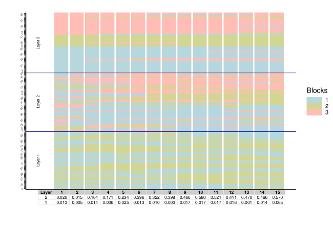
Figure D.11: Membership dynamics of nodes (different colors) in the different layers (vertical axis) for 15 periods (horizontal axis) in the unidirectional causality setting (Example 1).

Note: The nodes are sorted based on its membership on $\ell=3$ and $t=1$. The table below is the the Adjusted Rand Index (ARI) of the given period and layer with respect to $\ell=3$.

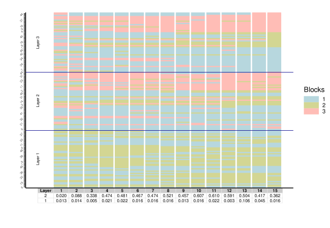
Figure D.12: Membership dynamics of the nodes in the different layers (vertical axis) for 15 periods (horizontal axis) in the bidirectional causality setting (Example 2).

Note: The nodes are sorted based on its membership on $\ell=3$ and $t=15$. The table below is the the Adjusted Rand Index (ARI) of the given period and layer with respect to $\ell=3$.

Figure D.13: Evolution of the network for Layer 2 and 3 at period 1 and 15 with membership variation (color) and node–specific membership persistence across layers (size of nodes) in the unidirectional causality setting (Example 1).

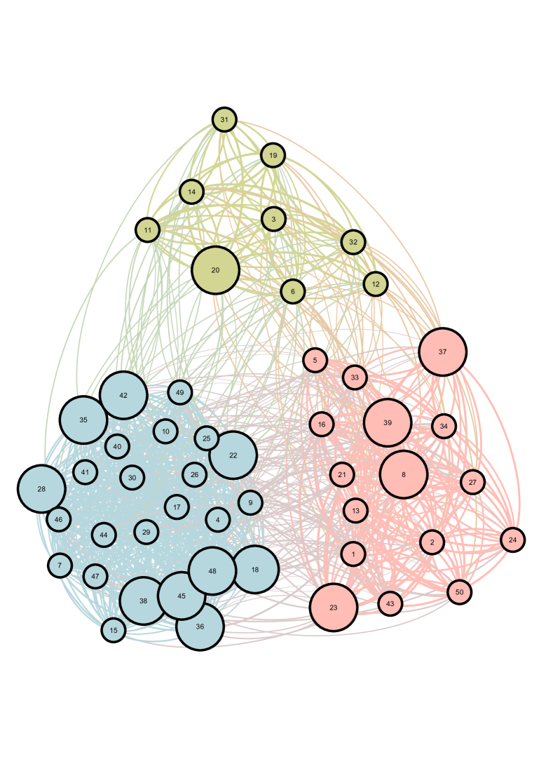
(a) $\ell=2$ and $t=1$

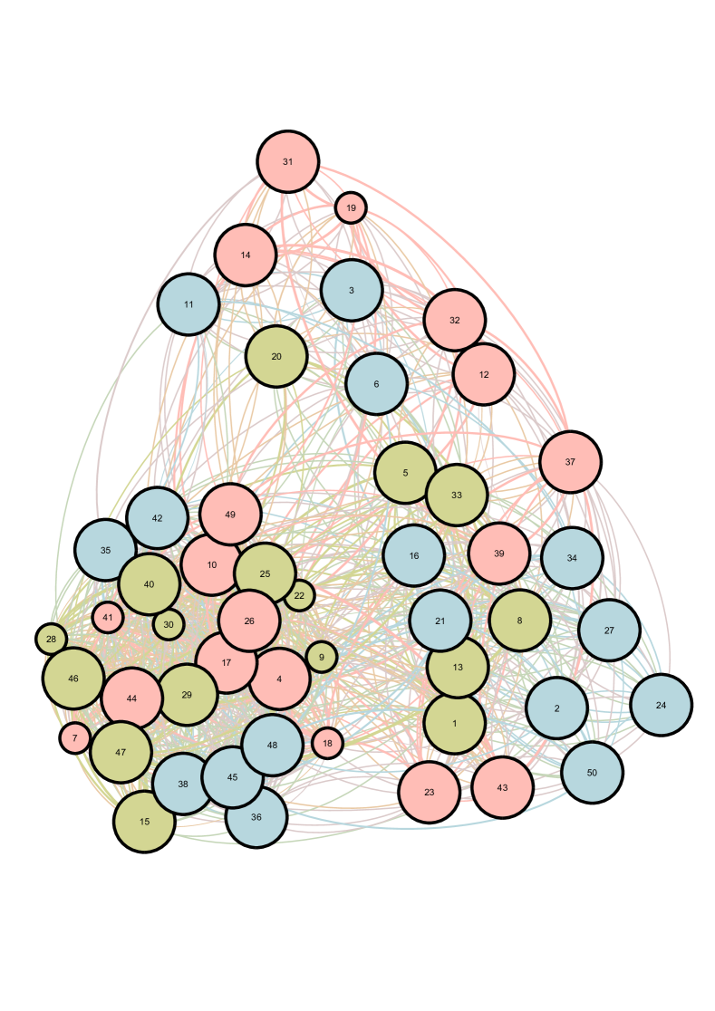
(b) $\ell=2$ and $t=15$

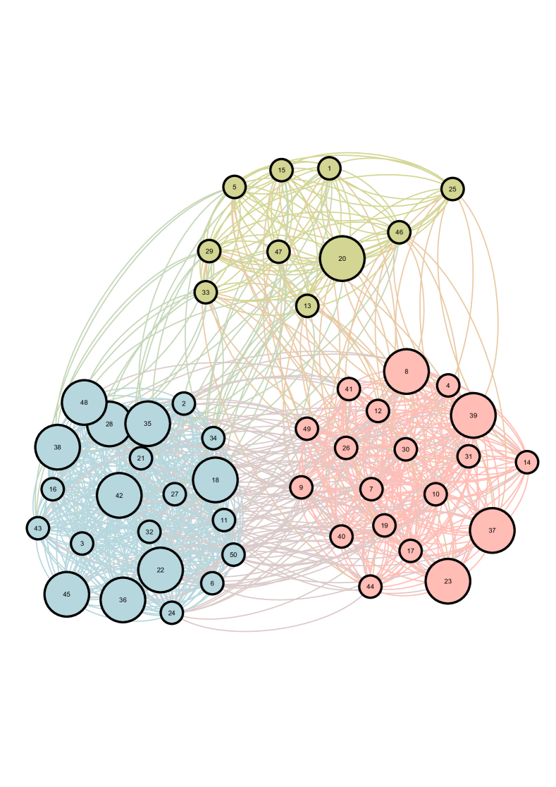
(c) $\ell=3$ and $t=1$

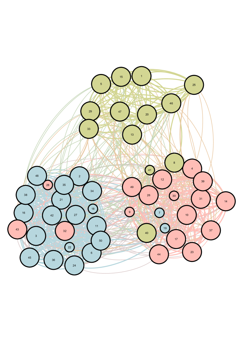
(d) $\ell=3$ and $t=15$

Note: The size of each node in Layer 2 (3) depends on its membership persistence (MP) with respect to Layer 3 (2), $MP^{(2)}_{it}=\mathbb{I}_{Z^{(2)}_{it}}\left(Z^{(3)}_{it}\right)$ and $MP^{(3)}_{it}=\mathbb{I}_{Z^{(3)}_{it}}\left(Z^{(2)}_{it}\right)$ respectively, either the node has a standard size or it is doubled.

Figure D.14: Evolution of the Network for Layer 2 and 3 at period 1 and 15 with membership variation (color) and node–specific membership persistence across layers (size of nodes) in the bidirectional causality setting (Example 2).

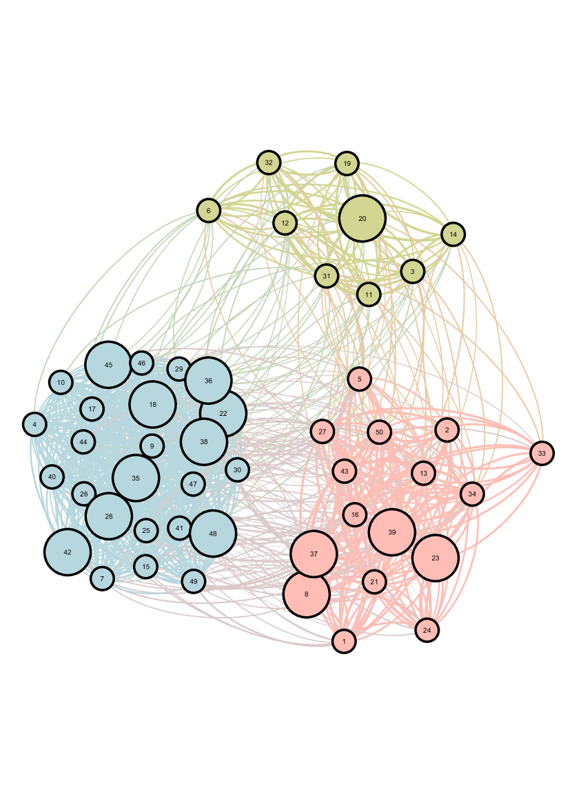
(a) $\ell=2$ and $t=1$

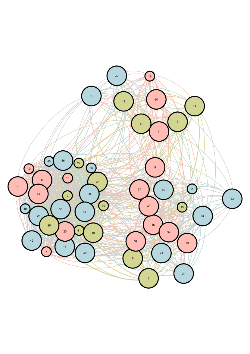
(b) $\ell=2$ and $t=15$

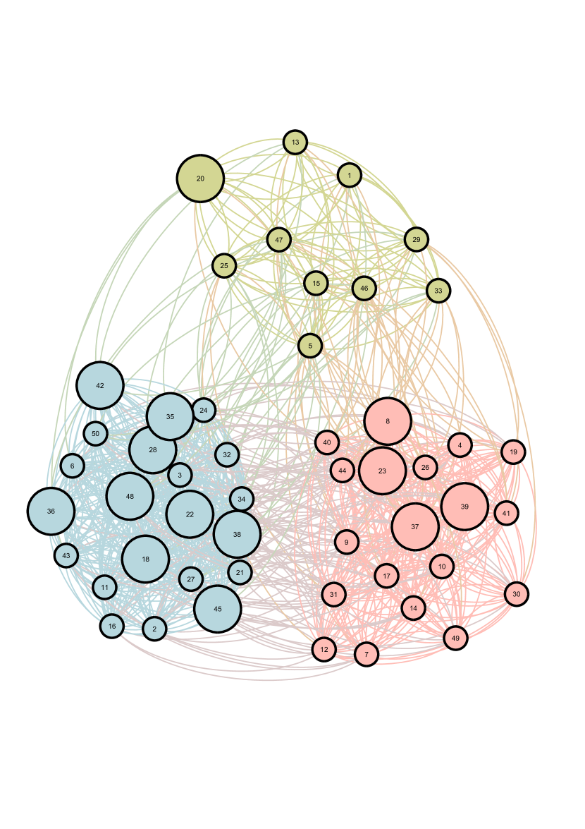
(c) $\ell=3$ and $t=1$

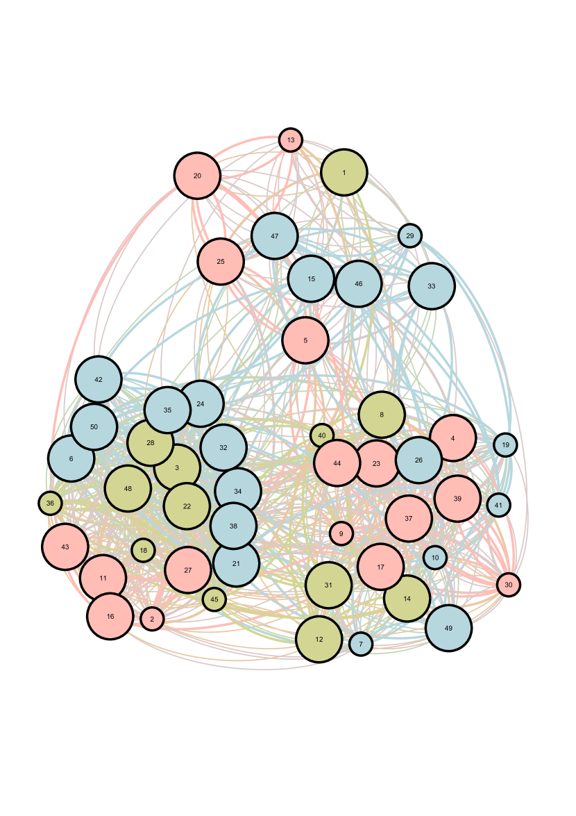
(d) $\ell=3$ and $t=15$

Note: The size of each node in Layer 2 (3) depends on its membership persistence (MP) with respect to Layer 3 (2), $MP^{(2)}_{it}=\mathbb{I}_{Z^{(2)}_{it}}\left(Z^{(3)}_{it}\right)$ and $MP^{(3)}_{it}=\mathbb{I}_{Z^{(3)}_{it}}\left(Z^{(2)}_{it}\right)$ respectively, either the node has a standard size or it is doubled.

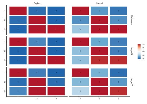
Figure D.15: Proportion of datasets (color) with evidence of Granger–causality in the block structure between different layers (rows and columns), under Normal and Group–Lasso Priors (super–columns) and various sample size set-ups (super–rows) in the unidirectional causality setting (Example 1) whose correct causality is denoted by the numbers in each rectangle.

Note: Reference sample size is $N=50$ and $T=15$, Larger $N$ is $N=100$ and $T=15$ and Larger $T$ is $N=50$ and $T=30$. The number of datasets generated in each scenario is 48. In each dataset the number of iterations is 2000 and a burn–in of 1000.

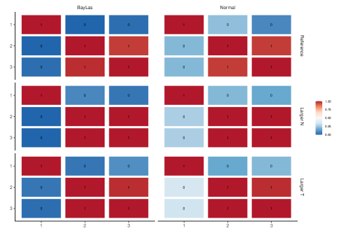
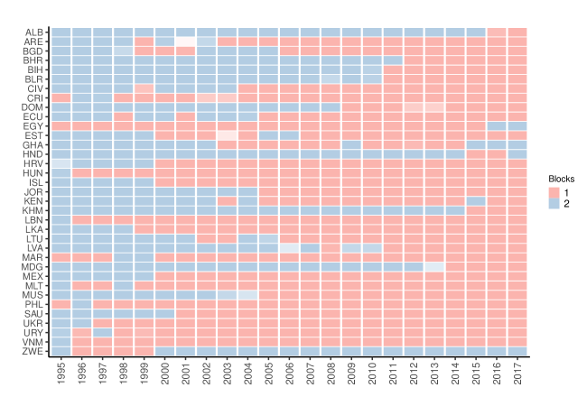
Figure D.16: Proportion of datasets (color) with evidence of Granger–causality in the block structure between different layers (rows and columns), under Normal and Group Lasso Priors (super–columns) and various sample size set-ups (super–rows) in the bidirectional causality setting (Example 2) whose correct causality is denoted by the numbers in each rectangle.

Note: Reference sample size is $N=50$ and $T=15$, Larger $N$ is $N=100$ and $T=15$ and Larger $T$ is $N=50$ and $T=30$. The number of datasets generated in each scenario is 48. In each dataset the number of iterations is 2000 and a burn–in of 1000.

Figure D.17: Changes in membership in the Trade Layer

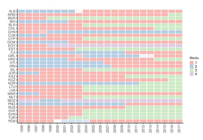
Figure D.18: Changes in Membership in the FTA network

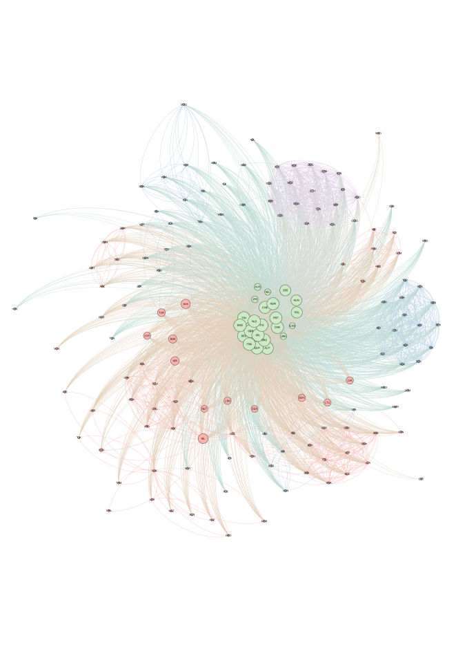
Figure D.19: FTA community structure 1995

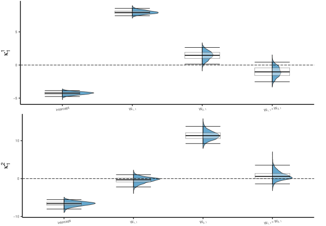
Figure D.20: Empirical density of the posterior distribution for transition probability parameters of the multinomial model for the Trade (Layer 1) and FTAs (Layer 2) network using as reference equation $Q^{(1)}=Q^{(2)}=2$

Note: Number of simulations: 30,000 and burn-in: 10,000. Thinning: 10.

References

- [1] Alan Agresti “Categorical data analysis” John Wiley & Sons, 2003
- [2] Komla M. Agudze, Monica Billio, Roberto Casarin and Francesco Ravazzolo “Markov switching panel with endogenous synchronization effects” In Journal of Econometrics, 2021
- [3] Edoardo M Airoldi, David M Blei, Stephen E Fienberg and Eric P Xing “Mixed membership stochastic blockmodels” In Journal of Machine Learning Research 9.Sep, 2008, pp. 1981–2014
- [4] Alberto Aleta and Yamir Moreno “Multilayer networks in a nutshell” In Annual Review of Condensed Matter Physics 10 Annual Reviews, 2019, pp. 45–62
- [5] James E Anderson “The gravity model” In Annu. Rev. Econ. 3.1 Annual Reviews, 2011, pp. 133–160
- [6] S. Baccaletti et al. “The structure and dynamics of multilayer networks” In Physics Reports 544.1, 2014, pp. 1–122
- [7] Scott L Baier and Jeffrey H Bergstrand “Economic determinants of free trade agreements” In Journal of International Economics 64.1 Elsevier, 2004, pp. 29–63
- [8] Scott L Baier and Jeffrey H Bergstrand “Do free trade agreements actually increase members’ international trade?” In Journal of International Economics 71.1 Elsevier, 2007, pp. 72–95
- [9] Scott L Baier, Yoto V Yotov and Thomas Zylkin “On the widely differing effects of free trade agreements: Lessons from twenty years of trade integration” In Journal of International Economics 116 Elsevier, 2019, pp. 206–226
- [10] Badi H Baltagi, Peter Egger and Michael Pfaffermayr “Estimating regional trade agreement effects on FDI in an interdependent world” In Journal of Econometrics 145.1-2 Elsevier, 2008, pp. 194–208
- [11] A.-L. Barabási and R. Albert “Emergence of scaling in random networks” In Science 286.5439, 1999, pp. 509–512
- [12] Leonardo Bargigli et al. “The multiplex structure of interbank networks” In Quantitative Finance 15.4 Taylor & Francis, 2015, pp. 673–691
- [13] Matteo Barigozzi, Giorgio Fagiolo and Giuseppe Mangioni “Identifying the community structure of the international-trade multi-network” In Physica A: Statistical Mechanics and its Applications 390.11 Elsevier, 2011, pp. 2051–2066
- [14] Paolo Bartesaghi, Gian Paolo Clemente and Rosanna Grassi “Communicability in the world trade network–a new perspective for community detection” In Journal of Economic Interaction and Coordination, 2020
- [15] Kristian Behrens, Cem Ertur and Wilfried Koch “‘Dual’gravity: Using spatial econometrics to control for multilateral resistance” In Journal of Applied Econometrics 27.5 Wiley Online Library, 2012, pp. 773–794
- [16] Andrew B Bernard, J Bradford Jensen, Stephen J Redding and Peter K Schott “Firms in international trade” In Journal of Economic Perspectives 21.3, 2007, pp. 105–130
- [17] Monica Billio, Roberto Casarin, Francesco Ravazzolo and Herman K Van Dijk “Interconnections between eurozone and US booms and busts using a Bayesian panel Markov-switching VAR model” In Journal of Applied Econometrics 31.7 Wiley Online Library, 2016, pp. 1352–1370
- [18] Bela Bollobas “Random Graphs” New York: Cambridge University Press, 2001
- [19] Fabio Canova and Matteo Ciccarelli “Panel Vector Autoregressive Models: A Survey” Emerald Group Publishing Limited, 2013
- [20] Gilles Celeux, Florence Forbes, Christian P Robert and D Mike Titterington “Deviance information criteria for missing data models” In Bayesian Analysis 1.4 International Society for Bayesian Analysis, 2006, pp. 651–673
- [21] Peter Csermely, András London, Ling-Yun Wu and Brian Uzzi “Structure and dynamics of core/periphery networks” In Journal of Complex Networks 1.2 Oxford University Press, 2013, pp. 93–123
- [22] Corinne Dahinden, Giovanni Parmigiani, Mark C Emerick and Peter Bühlmann “Penalized likelihood for sparse contingency tables with an application to full-length cDNA libraries” In BMC Bioinformatics 8.1 BioMed Central, 2007, pp. 1–11
- [23] Aureo De Paula “Econometrics of network models” In Advances in Economics and Econometrics: Theory and Applications, Eleventh World Congress, 2017, pp. 268–323 Cambridge University Press Cambridge
- [24] Alistair Dieppe, Romain Legrand and Björn Van Roye “The BEAR toolbox” ECB working paper, 2016
- [25] Mr Robert Dippelsman, Mr Marco Marini and Mr Michael Stanger “New estimates for Direction of Trade Statistics”, 2018
- [26] Jean-Marie Dufour and Abderrahim Taamouti “Short and long run causality measures: Theory and inference” In Journal of Econometrics 154.1 Elsevier, 2010, pp. 42–58
- [27] Peter H Egger, Mario Larch and Yoto V Yotov “Gravity-Model Estimation with Time-Interval Data: Revisiting the Impact of Free Trade Agreements”, 2020
- [28] Paul Erdős and Alfréd Rényi “On Random Graphs I.” In Publicationes Mathematicae (Debrecen) 6, 1959, pp. 290–297
- [29] Brian S Everitt “The analysis of contingency tables” CRC Press, 1992
- [30] Giorgio Fagiolo and Marina Mastrorillo “Does human migration affect international trade? A complex-network perspective” In PloS one 9.5 Public Library of Science, 2014
- [31] Sylvia Frühwirth-Schnatter “Label switching under model uncertainty” In Mixtures: Estimation and Application Citeseer, 2011, pp. 213–239
- [32] Sylvia Frühwirth-Schnatter and Rudolf Frühwirth “Data augmentation and MCMC for binary and multinomial logit models” In Statistical Modelling and Regression Structures Springer, 2010, pp. 111–132
- [33] Clive WJ Granger “Investigating causal relations by econometric models and cross-spectral methods” In Econometrica: Journal of the Econometric Society JSTOR, 1969, pp. 424–438
- [34] Tamara Gurevich and Peter Herman “The dynamic Gravity dataset: Technical documentation” Washington, DC: US International Trade Commission, 2018
- [35] James Hamilton “Time Series Analysis” Princeton: Princeton University Press, 1994
- [36] Qiuyi Han, Kevin Xu and Edoardo Airoldi “Consistent estimation of dynamic and multi-layer block models” In International Conference on Machine Learning, 2015, pp. 1511–1520
- [37] James J Heckman “Sample selection bias as a specification error” In Econometrica: Journal of the Econometric Society JSTOR, 1979, pp. 153–161
- [38] Leonhard Held and Chris C Holmes “Bayesian auxiliary variable models for binary and multinomial regression” In Bayesian Analysis 1.1 International Society for Bayesian Analysis, 2006, pp. 145–168
- [39] Elhanan Helpman, Marc Melitz and Yona Rubinstein “Estimating trade flows: Trading partners and trading volumes” In The Quarterly Journal of Economics 123.2 MIT Press, 2008, pp. 441–487
- [40] P. Hoff “Additive and multiplicative effects network models” In Statist. Sci. 36.1, 2021, pp. 34–50 arXiv:arXiv:1807.08038 [stat.ME]
- [41] Tracy Holsclaw, Arthur M Greene, Andrew W Robertson and Padhraic Smyth “Bayesian nonhomogeneous Markov models via Pólya-Gamma data augmentation with applications to rainfall modeling” In The Annals of Applied Statistics 11.1 Institute of Mathematical Statistics, 2017, pp. 393–426
- [42] Jianwei Hu, Hong Qin, Ting Yan and Yunpeng Zhao “Corrected Bayesian information criterion for stochastic block models” In Journal of the American Statistical Association 115.532 Taylor & Francis, 2020, pp. 1771–1783
- [43] Sanqing Hu et al. “Shortcomings/limitations of blockwise Granger causality and advances of blockwise new causality” In IEEE Transactions on Neural Networks and Learning Systems 27.12 IEEE, 2015, pp. 2588–2601
- [44] Lawrence Hubert and Phipps Arabie “Comparing partitions” In Journal of Classification 2.1 Springer, 1985, pp. 193–218
- [45] Artjoms Ivlevs and Jaime De Melo “FDI, the brain drain and trade: channels and evidence” In Annals of Economics and Statistics/Annales d’Économie et de Statistique JSTOR, 2010, pp. 103–121
- [46] Ajay Jasra, Chris C Holmes and David A Stephens “Markov chain Monte Carlo methods and the label switching problem in Bayesian mixture modeling” In Statistical Science JSTOR, 2005, pp. 50–67
- [47] Petar Jovanovski and Ljupco Kocarev “Bayesian consensus clustering in multiplex networks” In Chaos: An Interdisciplinary Journal of Nonlinear Science 29.10 AIP Publishing LLC, 2019, pp. 103142
- [48] Mahfuz Kabir, Ruhul Salim and Nasser Al-Mawali “The gravity model and trade flows: Recent developments in econometric modeling and empirical evidence” In Economic Analysis and Policy 56 Elsevier, 2017, pp. 60–71
- [49] Safaa K Kadhem, Paul Hewson and Irene Kaimi “Recursive Deviance Information Criterion for the Hidden Markov model” In International Journal of Statistics and Probability 5.1, 2016
- [50] Sylvia Kaufmann “K-state switching models with time-varying transition distributions—Does loan growth signal stronger effects of variables on inflation?” In Journal of Econometrics 187.1 Elsevier, 2015, pp. 82–94
- [51] Bomin Kim, Kevin H Lee, Lingzhou Xue and Xiaoyue Niu “A review of dynamic network models with latent variables” In Statistics Surveys 12 NIH Public Access, 2018, pp. 105
- [52] Changjin Kim and Charles R Nelson “State-space models with regime switching: classical and Gibbs-sampling approaches with applications” In MIT Press Books 1 The MIT press, 1999
- [53] Mikko Kivelä et al. “Multilayer networks” In Journal of Complex Networks 2.3, 2014, pp. 203–271
- [54] Gary M Koop “Forecasting with medium and large Bayesian VARs” In Journal of Applied Econometrics 28.2 Wiley Online Library, 2013, pp. 177–203
- [55] John K Kruschke “Rejecting or accepting parameter values in Bayesian estimation” In Advances in Methods and Practices in Psychological Science 1.2 Sage Publications Sage CA: Los Angeles, CA, 2018, pp. 270–280
- [56] Clement Lee and Darren J Wilkinson “A review of stochastic block models and extensions for graph clustering” In Applied Network Science 4.1 SpringerOpen, 2019, pp. 1–50
- [57] Kyu-Min Lee, B. Min and K-I Goh “Towards real-world complexity: An introduction to multiplex networks” In The European Physical Journal B 88.48, 2015
- [58] Jing Lei and Kevin Z Lin “Bias-adjusted spectral clustering in multi-layer stochastic block models” In Journal of the American Statistical Association Taylor & Francis, 2022, pp. 1–13
- [59] Glenn Magerman, Karolien De Bruyne and Jan Van Hove “Pecking order and core-periphery in international trade” In Review of International Economics 28.4 Wiley Online Library, 2020, pp. 1113–1141
- [60] Mahendra Mariadassou, Stéphane Robin and Corinne Vacher “Uncovering latent structure in valued graphs: a variational approach” In The Annals of Applied Statistics 4.2 Institute of Mathematical Statistics, 2010, pp. 715–742
- [61] James R Markusen “Multinational firms and the theory of international trade” MIT press, 2002
- [62] Catherine Matias and Vincent Miele “Statistical clustering of temporal networks through a dynamic stochastic block model” In Journal of the Royal Statistical Society: Series B (Statistical Methodology) 79.4 Wiley Online Library, 2017, pp. 1119–1141
- [63] Rocco Mosconi and Raffaello Seri “Non-causality in bivariate binary time series” In Journal of Econometrics 132.2 Elsevier, 2006, pp. 379–407
- [64] Mark Newman “Networks: An introduction” Oxford University Press, 2010, pp. 772
- [65] James R Norris “Markov chains” Cambridge University Press, 1998
- [66] Santiago Olivella, Tyler Pratt and Kosuke Imai “Dynamic Stochastic Blockmodel Regression for Social Networks: Application to International Conflicts”, 2018
- [67] Edoardo Otranto “The multi-chain Markov switching model” In Journal of Forecasting 24.7 Wiley Online Library, 2005, pp. 523–537
- [68] Trevor Park and George Casella “The Bayesian lasso” In Journal of the American Statistical Association 103.482 Taylor & Francis, 2008, pp. 681–686
- [69] Subhadeep Paul and Yuguo Chen “A random effects stochastic block model for joint community detection in multiple networks with applications to neuroimaging” In The Annals of Applied Statistics 14.2 Institute of Mathematical Statistics, 2020, pp. 993–1029
- [70] R Piermartini and YV Yotov “Estimating trade policy effects with structural gravity”, 2016
- [71] Nicholas G Polson, James G Scott and Jesse Windle “Bayesian inference for logistic models using Pólya–Gamma latent variables” In Journal of the American Statistical Association 108.504 Taylor & Francis, 2013, pp. 1339–1349
- [72] Sudhir Raman et al. “The Bayesian group-lasso for analyzing contingency tables” In Proceedings of the 26th Annual International Conference on Machine Learning, 2009, pp. 881–888
- [73] Michael Salter-Townshend and Tyler H McCormick “Latent space models for multiview network data” In The Annals of Applied Statistics 11.3 NIH Public Access, 2017, pp. 1217
- [74] Patrick Schwaferts and Thomas Augustin “Bayesian decisions using Regions of Practical Equivalence (ROPE): Foundations”, 2020
- [75] JMC Santos Silva and Silvana Tenreyro “The log of gravity” In The Review of Economics and Statistics 88.4 The MIT Press, 2006, pp. 641–658
- [76] Christopher A Sims “Macroeconomics and reality” In Econometrica: Journal of the Econometric Society JSTOR, 1980, pp. 1–48
- [77] Silvia Sopranzetti “Overlapping free trade agreements and international trade: A network approach” In The World Economy 41.6 Wiley Online Library, 2018, pp. 1549–1566
- [78] Natalie Stanley, Saray Shai, Dane Taylor and Peter J Mucha “Clustering network layers with the strata multilayer stochastic block model” In IEEE Transactions on Network Science and Engineering 3.2 IEEE, 2016, pp. 95–105
- [79] Tracy M Sweet “Incorporating covariates into stochastic blockmodels” In Journal of Educational and Behavioral Statistics 40.6 SAGE Publications Sage CA: Los Angeles, CA, 2015, pp. 635–664
- [80] Jan Tinbergen “Shaping the world economy the twentieth century Fund” In New York 330, 1962
- [81] Martijn Van Hasselt “Bayesian inference in a sample selection model” In Journal of Econometrics 165.2 Elsevier, 2011, pp. 221–232
- [82] D.. Watts and S.. Strogatz “Collective dynamics of ’small-world’ networks” In Nature 393, 1998, pp. 440–442
- [83] Xiaoran Yan “Bayesian model selection of stochastic block models” In 2016 IEEE/ACM International Conference on Advances in Social Networks Analysis and Mining (ASONAM), 2016, pp. 323–328 IEEE
- [84] Tianbao Yang et al. “Detecting communities and their evolutions in dynamic social networks—a Bayesian approach” In Machine Learning 82.2 Springer, 2011, pp. 157–189
- [85] Ming Yuan and Yi Lin “Model selection and estimation in regression with grouped variables” In Journal of the Royal Statistical Society: Series B (Statistical Methodology) 68.1 Wiley Online Library, 2006, pp. 49–67
- [86] Yunpeng Zhao, Elizaveta Levina and Ji Zhu “Consistency of community detection in networks under degree-corrected stochastic block models” In The Annals of Statistics 40.4 Institute of Mathematical Statistics, 2012, pp. 2266–2292