An Exploration of Systematic Errors in Transiting Planets and Their Host Stars

Abstract

Transiting planet systems offer the best opportunity to measure the masses and radii of a large sample of planets and their host stars. However, relative photometry and radial velocity measurements alone only constrain the density of the host star. Thus, there is a one-parameter degeneracy in the mass and radius of the host star, and by extension the planet. Several theoretical, semi-empirical, and nearly empirical methods have been used to break this degeneracy and independently measure the mass and radius of the host star and planets(s). As we approach an era of few percent precisions on some of these properties, it is critical to assess whether these different methods are providing accuracies that are of the same order, or better than, the stated statistical precisions. We investigate the differences in the planet parameter estimates inferred when using the Torres empirical relations, YY isochrones, MIST isochrones, and a nearly-direct empirical measurement of the radius of the host star using its spectral energy distribution, effective temperature, and Gaia parallax. We focus our analysis on modelling KELT-15b, a fairly typical hot Jupiter, using each of these methods. We globally model TESS photometry, optical-to-NIR flux densities of the host star, and Gaia parallaxes, in conjunction with extant KELT ground-based follow-up photometric and radial velocity measurements. We find systematic differences in several of the inferred parameters of the KELT-15 system when using different methods, including a $\sim 6\%$ ($\sim 2\sigma$) difference in the inferred stellar and planetary radii between the MIST isochrones and SED fitting.

1 Introduction

Accurate masses and radii are generally needed to determine the basic nature of exoplanets. For example, estimates of the densities of exoplanets from their measured masses and radii have led to the discovery of previously unknown classes of planets such as “Super Earths,” “Sub-Neptunes,” and ultra low-density “Puffballs.” Indeed, the density determination of the first transiting planet detected, HD209458b (Charbonneau et al., 2000) showed conclusively that Hot Jupiters such as 51 Peg b (Mayor & Queloz, 1995) were confirmed planets with densities similar to the giant planets in our solar system. Moreover, precise and accurate masses and radii of planets are needed to perform detailed comparative exoplanetology, which ultimately can be used to help our understanding of the formation and evolution of planetary systems.

Determining both masses and radii of planets can essentially only be done for transiting planets. However, even with arbitrarily precise measurements of the photometry and radial velocity (RV) of transiting planets, it is not possible to independently determine the mass $M_{\star}$ and radius $R_{\star}$ of the host star or the mass $M_{P}$ and radius $M_{P}$ of its transiting planets. This is because these measurements alone do not constrain the absolute mass or size scale of the system. Rather, these measurements can only be used to determine the density of the star, $\rho_{*}$ (Seager & Mallén-Ornelas, 2003), resulting in a one-parameter degeneracy that must be broken to set the scale of the system and measure the absolute masses and radii of the host star and planets.

Directly observable parameters are those that can be determined purely from photometric and RV observations. Such parameters include the planet period $P$, transit depth $\delta$, the full-width at half-maximum of the transit duration $T_{\rm FWHM}$, the ingress/egress duration $\tau$, and the eccentricity $e$, argument of periastron $\omega$ and semi-amplitude $K_{*}$ of the RV observations. From these observables, the semi-major axis of the planet orbit scaled to the radius of the star $a/R_{*}$ can be determined, as well as the surface gravity of the planet $g_{P}$. The parallax $\pi_{\star}$ of the star can also be measured, which, combined with the spectral energy distribution (SED) and effective temperature $T_{\rm eff}$ of the host star, can be used to constrain the stellar radius $R_{\star}$.

The planet mass $M_{p}$ can be inferred from $M_{\star}$ and the RV semi-amplitude $K_{\star}$ the star via

$$K=\left(\frac{2\pi G}{P}\right)^{1/3}\frac{M_{p}\sin{i}}{(M_{\star}+M_{p})^{2/3}}\frac{1}{\sqrt{1-e^{2}}},$$ (1)

where precise shape of the RV curve can be used to measure $e$, and inclination of the orbit $i$ can be determined from the light curve. Thus by measuring $K_{\star}$, we establish a relationship between $M_{*}$ and $M_{p}$ which depends only on the directly observable parameters $K$, $e$, $i$ and $P$.

Similarly, the planet radius $R_{P}$ can be inferred from $R_{*}$ and the transit depth

$$\delta=\left(\frac{R_{P}}{R_{\star}}\right)^{2},$$ (2)

which can be measured more-or-less directly from the relative photometry of the host star during transits. Thus $\delta$ serves as a direct observable that establishes a relationship between $R_{*}$ and $R_{p}$.

However, it is not possible to estimate absolute values for $R_{*}$ and $M_{*}$ through the relative photometric measurements of the transit or the RV observations alone. Direct observables can provide a relationship between the semi-major axis a and $R_{*}$ shown in equation 3,

$$\frac{a}{R_{*}}=\frac{\delta^{1/4}}{\pi}\frac{P}{\sqrt{T_{FWHM}\tau}}\left(\frac{\sqrt{1-e^{2}}}{1+e\sin\omega}\right).$$ (3)

This dimensionless factor can also be used to derive a relationship the density of the host star $\rho_{*}$ and the surface gravity of the planet $g_{p}$ solely in terms of direct observables. The density of the star is given by

$$\rho_{\star}=\frac{3\pi}{GP^{2}}\left(\frac{a}{R_{\star}}\right)^{3}-k^{3}\rho_{p}\simeq\frac{3\pi}{GP^{2}}\left(\frac{a}{R_{\star}}\right)^{3},$$ (4)

where $k\equiv R_{p}/R_{*}$. For transiting planets, $k\ll 1$ and $\rho_{p}\sim\rho_{*}$, justifying the second approximation. The surface gravity of the planet is given by,

$$g_{p}=\frac{2K_{\star}P}{\pi T\tau}\delta^{-1/2}.$$ (5)

Thus there is still a one-parameter degeneracy between $R_{*}$ and $M_{*}$. By extension, this also implies that the mass and radius of the exoplanet can not be determined with only photometric and RV observations. Additional information must be introduced to break this degeneracy and fully characterise both the host star and the exoplanet.

Four primary methods are commonly used to break this mass-radius degeneracy. Two suites of theoretical stellar evolutionary models (Dotter, 2016; Yi et al., 2001) are often combined with other empirical information about the host star (e.g., $T_{\rm eff}$, $\log{g_{*}}$, [Fe/H]). Next, one can apply empirical relations between the mass and radius of the star and its surface gravity (or density), effective temperature, and metallicity (Torres et al., 2009; Enoch et al., 2010). Finally, the radius of the host star can be estimated using its Spectral Energy Distribution (SED) and distance from parallax (Stassun et al., 2017). All four methods have their advantages and disadvantages, and these are generally complementary. All four have been used to infer the mass and radius in published discoveries of transiting planets. Thus the ensemble of known transiting planets represent a sample whose properties were inferred in an inhomogenous way. Furthermore, to date there have been very few comparisons between the parameters inferred using these different methods of breaking the degeneracy. Therefore, while we may know the precision of the reported mass and radius measurements of transiting planets, we generally do not know the accuracy of these parameters, and particularly whether the accuracy exceeds the quoted precision in some subset of cases.

These four methods previously discussed are not the only ones currently in use. If the radius of the host star can be measured independently through other means (Kjeldsen & Bedding (1995); Bastien et al. (2013)), this can also break the degeneracy. Stevens et al. (2018) analytically estimated the precision of model independent masses and radii for exoplanet systems with transit photometry and radial velocity observations. End of mission Gaia will provide parallaxes with uncertainty in the $5-10\mu\rm as$ range which will translate to stellar radii to as uncertainties of a few percent (Gaia Collaboration et al., 2016a). Stevens et al. (2018) showed that these parallaxes will allow for stellar masses and radii for single-lined eclipsing binaries that will be nearly model independent. Through another approach, spectroscopic stellar surface gravity measurements can provide a direct estimate of $\log{g_{*}}$ and thus derive $R_{*}$. However, this type of measurement requires high spectral resolution ($\rm R\geq 50,000$). The estimates of $\log{g_{*}}$ produced by this method are often neither very precise or accurate (Heiter et al., 2015; Mortier et al., 2014). Alternatively, there are other indirect methods to estimate $\log{g_{*}}$ such as flicker-based surface gravity measurements. Granulation on the surface of stars can produce variations in flux, or flicker, which has been shown to be strongly correlated with $\log{g_{*}}$ (Bastien et al., 2013, 2016). However the relationship between $\log{g_{*}}$ and $R_{*}$ requires calibration which introduces more sources of uncertainty. Asteroseismology can provide another avenue of estimating $R_{*}$ and $M_{*}$. Acoustic oscillations in stars produce a power spectrum of brightness fluctuations. The large frequency spacing of the peaks in the power spectrum $\delta v$ is directly related to $\rho_{*}$, whereas the frequency of the maximum power $\nu_{\rm max}$, is related to $\log{g_{*}}$ and $T_{\rm eff}$ via an empirically calibrated scaling relation (Kjeldsen & Bedding, 1995). These parameters can be combined for an indirect estimate of $R_{*}$ and $M_{*}$. However, both asteroseismology and flicker measurements both require high-cadence, high-precision light curve observations with long baselines such as those from Kepler (Borucki et al., 2010). Asteroseismic techniques have been applied to several exoplanet host stars (Huber et al., 2022; Jiang et al., 2020). However, these observations would be difficult to obtain for many of the stars hosting transiting planets. Thus these methods are not included in this study.

Here, we take a first step in assessing the accuracy of the parameters inferred using our four commonly used methods of breaking the mass-radius degeneracy. We consider KELT-15b (Rodriguez et al., 2016), a system with a bright star, known to host only a single transiting hot Jupiter. We fit this system using several different methods of breaking the mass-radius degeneracy. We use EXOFASTv2 (Eastman et al., 2019, 2012), which fits the photometric and radial velocity data of transiting planets, and allows the user to use theoretical, semi-empirical, or nearly empirical methods to break the mass-radius degeneracy in the host star and to determine masses and radii for both the star and its planet.

EXOFASTv2 allows the user to adopt external constraints from the SED of the star, which when combined with the parallax and a constraint on the effective temperature, $T_{\rm eff}$ (either from the SED itself or from, e.g., high-resolution spectroscopy), yields the stellar radius (Eastman et al., 2012, 2019). EXOFASTv2 also supports the Torres empirical mass-radius relations (Torres et al., 2009), Yonsei-Yale evolutionary tracks (Yi et al., 2001), and the Mesa Isochrone and Stellar Track (MIST) models (Dotter, 2016) as methods of breaking the host star mass-radius degeneracy. In addition, EXOFASTv2 fits the photometric and radial velocity data of transiting planets system while simultaneously adopting one or more of these constraints.

The resulting inferred system parameters will depend to a larger or smaller extent on which of the above methods were used to break the mass - radius degeneracy. In addition, we will investigate the effects of removing or loosening some priors on the median values characterizing this system. Specifically, we consider removing the assumption of circular orbit, removing a prior on the limb darkening of the host star, and loosening the prior on the the stellar effective temperature $T_{\rm eff}$. In this way, we can determine how consistent the results are when adopting different priors. This will provide insight into the consistency and accuracy of the models, as well as the systematic errors on the inferred system parameters due to the choice of priors.

The plan for this paper is as follows. In Section 2, we summarize the four methods of breaking the host star mass-radius degeneracy which we will use to characterise KELT-15b. In Section 2.1, we provide the rationale for selecting KELT-15b as the test-bed of this analysis. In Section 3, check the robustness of our modelling procedure by reproducing the results from the original analysis of this system, Rodriguez et al. (2016). In Section 4, we outline our analysis approach to systematically model KELT-15b. In Section 5, we describe our results. In Section 6, we discuss the implications of these results on modeling transiting planets. Finally, in section 7, we summarize our findings and their impact.

2 Description of External Constraints Used by EXOFASTv2 

There are several common methods that use indirect constraints to break the mass and radius degeneracy in the host star. EXOFASTv2 can use broad band photometry to model the Spectral Energy Distribution (SED) of a star which provides a measure of the star’s bolometric flux (Eastman et al., 2019). The SED is mostly independent of stellar models (Stassun & Torres, 2016). This means it can be used in conjunction with the following models without double counting information about the star. We add the 0.082 mas systematic parallax offset found in the Gaia DR2 inferred by (Stassun & Torres, 2018). SED fitting should not be used if there is suspicion that its broad band photometry is blended with another star. The SED depends only weakly on the surface gravity $\log{g_{*}}$ and metallicity of the star, but does place constraints on $T_{\rm eff}$ and the $V$-band extinction, $A_{V}$. By fitting the SED, inferring $T_{\rm eff}$ from high-resolution spectra and estimating $A_{V}$, we can infer the bolometric flux, which when combined with $T_{\rm eff}$, yields the angular radius of the star, $(R_{*}/d)^{2}$. The stellar radius $R_{*}$ can then be inferred from the distance derived by the parallax (Stassun et al., 2017). Thus the SED and a parallax measurement can provide direct and empirical constrains on the radius of the host star.

Another approach is applying semi-empirical relationships, such as the the Torres relations (Torres et al., 2009). The study looked at 95 detached double-lined eclipsing binary systems (and the $\alpha$ Centauri system) and found empirical relationships between the mass and radii of these stars and $\log{g_{*}}$, $T_{\rm eff}$, and [Fe/H]. As is well known, double-lined eclipsing binary systems allow for accurate measurements of the mass and radii of both stars, without the need for an external constraint on the distance. The Torres relations applied primarily to unevolved or somewhat evolved main sequences stars. They do not apply to giants or pre main sequence stars. Furthermore, only a handful of the stars in the Torres et al. sample were low-mass M stars, and thus one should be wary of applying them to low-mass stars. Note that the Torres et al. relations yielded masses and radii that are accurate to 6% and 3 %, respectively, based on the scatter of the measured values of these quantities relative to those predicted by the relations. With measurements of $\log{g_{*}}$, $T_{\rm eff}$, and [Fe/H], these relations can be used to quickly estimate $M_{*}$ and $R_{*}$.

Stellar Evolutionary tracks are a popular indirect method of estimating stellar properties. The Yonsei-Yale (YY) stellar evolutionary tracks followed the evolution of stars from pre-main sequence to predict the luminosity, color, $T_{\rm eff}$, and radius as a function of mass, age, and metallicity of the star (Yi et al., 2001). We note that the YY evolutionary tracks used in EXOFASTv2 do not apply to stars less than $0.5~{}M_{\odot}$ (Eastman et al., 2019). In this study, the mass of our host star is roughly $1.2~{}M_{\odot}$, thus in the range where the YY evolutionary tracks are applicable.

The MESA Isochrone and Stellar Tracks (MIST) models (Dotter, 2016) are the default for EXOFASTv2 (Eastman et al., 2019). They attempted to characterize stars between $0.1~{}M_{\odot}$ to $300~{}M_{\odot}$, starting at 100,000 years in age, thus including pre-main sequence stars Dotter (2016). The stellar evolutionary tracks are computed using a grid of initial mass, initial [Fe/H], and evolutionary phase (Eastman et al., 2019).

Over the years, different methods have been used by different authors. Older ground based exoplanet surveys like WASP (Pollacco et al., 2006), HAT (Bakos et al., 2004), and KELT (Pepper et al., 2007, 2012) used different modeling methods throughout their lifespans with no consensus approach. However, no study exists in the literature comparing the systematic differences in median values of exoplanet properties using each of these methods.

Table 1: KELT-15 Parameters from Literature

Parameter	Description	Value	References
TYC	Tycho-2 Name	8146-86-1	Høg et al. (2000)
2MASS	2MASS Name	J07493960-5207136	Cutri et al. (2003)
TIC	TESS ID	268644785	Stassun et al. (2019)
$\alpha_{J2000}$	Right Ascension (R.A.)	07:49:39.606	Høg et al. (2000)
$\delta_{J2000}$	Declination (Decl.)	-52:07:13.58	Høg et al. (2000)
$\mu_{\alpha}$	Proper Motion in R.A. (mas yr-1)	$-3.4\pm 2.3$	Zacharias et al. (2004)
BT	Tycho BT mag	$11.889\pm 0.084$	Høg et al. (2000)
VT	Tycho VT mag	$11.44\pm 0.089$	Høg et al. (2000)
J	2MASS J mag	$10.205\pm 0.02$	Cutri et al. (2003)
H	2MASS H mag	$9.919\pm 0.02$	Cutri et al. (2003)
K	2MASS K mag	$9.854\pm 0.03$	Cutri et al. (2003)
WISE1	WISE1 mag	$9.787\pm 0.03$	Cutri et al. (2021)
WISE2	WISE2 mag	$9.817\pm 0.03$	Cutri et al. (2021)
WISE3	WISE3 mag	$9.787\pm 0.037$	Cutri et al. (2021)
GaiaGaia	Gaia mag	$11.069\pm 0.02$	Gaia Collaboration et al. (2016a)
GaiaBP	GaiaBP mag	$11.372\pm 0.02$	Gaia Collaboration et al. (2016a)
GaiaRP	GaiaRP mag	$10.631\pm 0.02$	Gaia Collaboration et al. (2016a)
$\mu_{\delta}$	Proper Motion in Decl. (mas yr-1)	$-2.0\pm 2.9$	Zacharias et al. (2004)
Distance	Estimated Distance (pc)	$291\pm 30$	Rodriguez et al. (2016)
RV	Absolute RV (km s-1)	$7.6\pm 0.4$	Rodriguez et al. (2016)
$M_{*}$	Mass($M_{\odot}$)	$1.181^{+0.051}_{-0.050}$	Rodriguez et al. (2016)
$R_{*}$	Radius($R_{\odot}$)	$1.481^{+0.091}_{-0.041}$	Rodriguez et al. (2016)
$L_{*}$	Luminosity ($L_{\odot}$)	$2.56^{+0.35}_{-0.20}$	Rodriguez et al. (2016)
Teff	Effective temperature (K)	$6003^{+56}_{-52}$	Rodriguez et al. (2016)
$\rm[Fe/H]$	Metallicity	$0.047\pm 0.032$	Rodriguez et al. (2016)

2.1 KELT-15 as a Test Case

We choose to analyze KELT-15 (Rodriguez et al., 2016) because it a relatively simple transiting Hot Jupiter system, but nevertheless has well-constrained parameters based on multiple ground based transit and radial velocity observations. KELT-15b was discovered by the the KELT (Kilodegree Extremely Little Telescope) survey (Pepper et al., 2007, 2012). The KELT survey observations triggered on planet candidates and recommended them for follow up by their network of associated observatories. Therefore, each of these planets were observed by several ground based observatories through both relative photometry and radial velocity observations. These ground based observations came from several sources. Photometery was obtained from KELT-South (Pepper et al., 2012), LCOGT (Brown et al., 2013), PEST Observatory (owned and operated by TG Tan), and Adelaide Observatory (owned and operated by Ivan Curtis). Radial velocity observations were provided by the CORALIE instrument at the ESO La Silla Observatory (Queloz et al., 2001) and and the Anglo-Australian Telescope (AAT) using the CYCLOPS2 instrument (Horton et al., 2012). Sections 2.1 and 2.2 of Rodriguez et al. (2016) provided details on the ground based photometry. Section 2.3 described the Spectroscopic Follow-up and radial velocity observations. KELT-15 was also observed by Transiting Exoplanet Survey Satellite TESS after its initial discovery, providing the means for a reanalysis to improve the precision on the system parameters.

KELT-15b is an excellent candidate based on a few criteria. Select parameters for this system are shown in table 1. It orbits a star that is not exceedingly hot ($T_{\rm eff}$ $\sim 7,000K$). Adaptive Optics observations with Keck did not show any evidence for a blended companion. The host star did not show high levels of activity. Finally, the mass of the host star was $\sim 1.2M_{\odot}$, where the Torres relations are still valid. Its host star was bright ($V=11.2$) (Høg et al., 2000), which allowed for follow up by TESS. The initial discovery paper also provided estimates for $\rm[Fe/H]$ and $T_{\rm eff}$ based on the analysis of high-resolution spectra. Rodriguez et al. (2016) determined that KELT-15 is a G0 type star which is roughly 4.6 Gyr in age. This would place it close to the “blue hook” evolutionary phase, right before the Hertzsprung gap (Rodriguez et al., 2016). In table 1 we also show the magnitude measurements used to construct our SED. These magnitude observations are the same observations used in Rodriguez et al. (2016) aside from the exclusion of the APASS magnitudes used in that study and the addition of the Gaia DR2 magnitude measurements included here.

Rodriguez et al. (2016) found that KELT-15b is a hot Jupiter with a radius of $1.443^{+0.110}_{-0.057}R_{J}$ and a roughly 3 day orbit. Stellar parameters were determined using Spectroscopy Made Easy (Valenti & Piskunov, 1996). The observations were originally fit using a modified version of the first iteration of EXOFAST (Eastman et al., 2012). The authors fit the system twice using constraints on the host star properties from the YY model in one fit and the Torres relations in another. They also found the eccentricity of the system to be consistent with zero within 2-$\sigma$.

In our analysis of KELT-15b we include recent TESS observations which were not available at the time of the discovery paper. TESS recorded two sets of observations in January and February of 2019 and three sets of observations from the early months of 2021. KELT-15b provides an excellent example of a hot Jupiter with significant follow up observations. Any variation produced by our analysis with different models will be purely produced by different assumptions in fitting the derived parameters as we expect our direct observables to be well constrained by these robust observations.

3 Validation of Fitting Technique and the Minimum Irreducible Systematic Error

We begin by using EXOFASTv2 to fit the data used in the KELT-15b discovery paper by Rodriguez et al. (2016). Specifically, we use the exact same observations and priors used by Rodriguez et al. (2016) to infer the parameters of the system. Thus, in principle, we would expect that the inferred parameters in our analysis would agree essentially perfectly or more precisely, by $\sim 0.05\sigma$ given the convergence level required by EXOFASTv2 as described in Eastman et al. (2019) Section 23.4, where $\sigma$ is the uncertainty on a parameter. The only source of the differences would be coming from numerical noise due to, e.g., the finite number of Markov Chain Monte Carlo (MCMC) steps used or Poisson fluctuations in the MCMC chains. This therefore provides a ‘sanity check’ to ensure that our analysis methodology is correct. However, we note that the initial analysis by Rodriguez et al. (2016) was conducted using the software package MultiFast, which is a somewhat altered and upgraded version of the original version of EXOFAST (Eastman et al., 2012). Different software packages can have subtle differences in, e.g., the fitting of limb darkening coefficients or the way that uncertainties are handled. We would expect these differences to be minor in this case, because both EXOFASTv2 and MultiFast are based heavily on the original EXOFAST software package. Nevertheless, we find subtle differences in some of the inferred parameters as shown in Figure 1. These can be thought of as the irreducible minimum systematic errors on these parameters; we expect the differences between parameters inferred by EXOFASTv2 and software packages with other heritage to be even larger. The work of Patel & Espinoza (2022) showed that limb darkening coefficients derived from model atmospheres can have a differences in $u_{2}$ as large as $\sim 0.2$ compared to empirically obtained limb darkening coefficients from TESS observations. If other packages use differing approaches to fitting limb darkening coefficients or handling uncertainties, we would expect corresponding differences in the characterization of the transiting exoplanet.

We note that the only priors used in the original Rodriguez et al. (2016) analysis and our analysis are on $T_{\rm eff}$, [Fe/H], and the period of the planet as estimated from KELT observations. The central values and $1\sigma$ uncertainties on the priors were identical in both analyses.

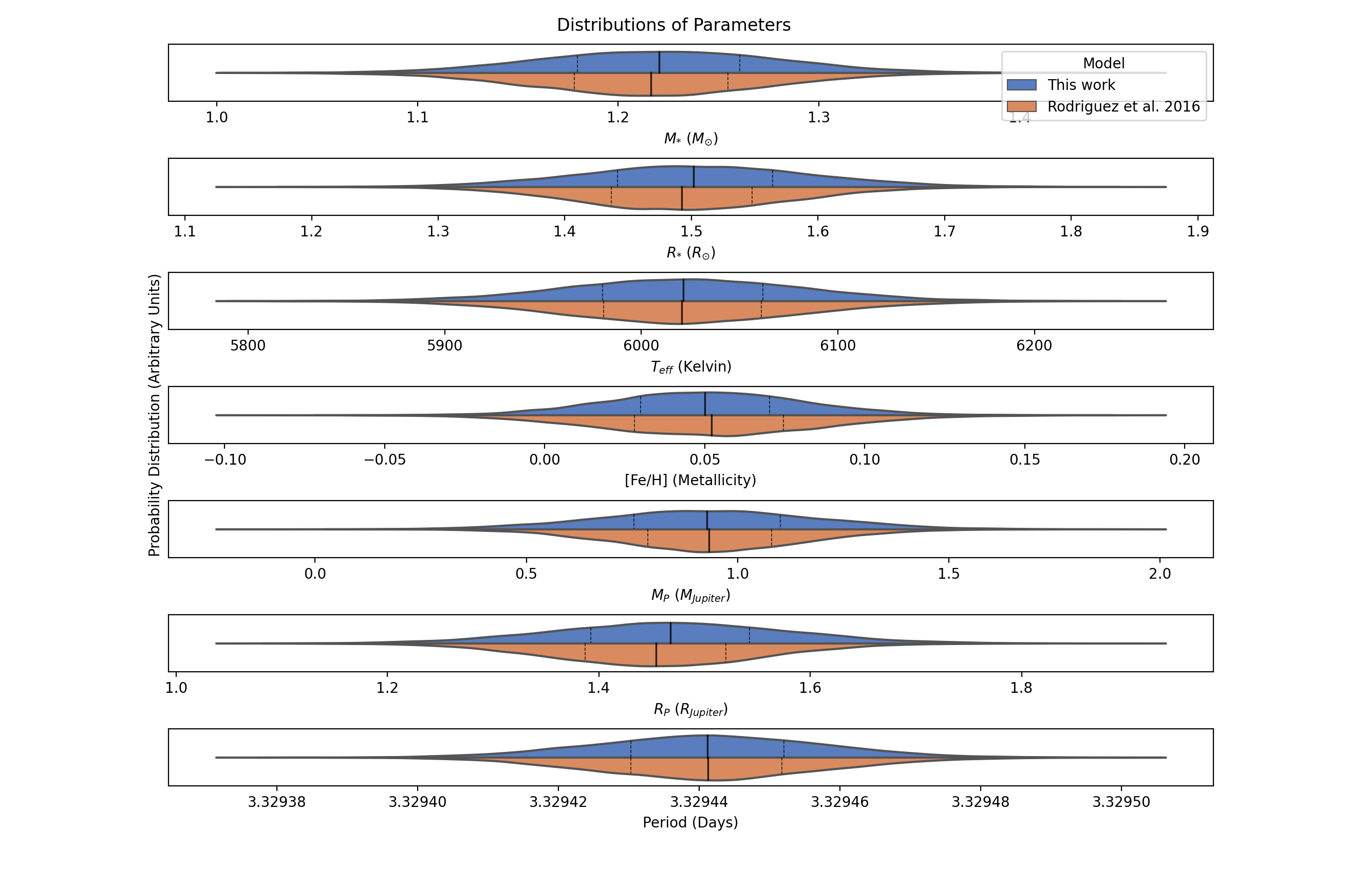
Figure 1: We represent the posterior distributions for the analysis of this work in blue and that of Rodriguez et al. (2016) in orange. The solid black line is the median value for each parameter. The dotted lines represent the inter-quartile range. The shaded region indicates the posterior distribution.

We compare this initial run to the case in Rodriguez et al. (2016) which assumes circular orbits and adopts the Torres relations as the mass-radius degeneracy breaking method (Torres et al., 2009). We fit KELT-15b using EXOFASTv2 on the same observations, and use the same priors as Rodriguez et al. (2016), apply the Torres relations, and assume circular orbits. The results of this trial are shown in Table 2 and Figure 1. In the last column, $\sigma$ is defined as the difference between our median value and the median value of Rodriguez et al. (2016) divided by the larger of the two uncertainties.

Table 2: Re-analysis of KELT-15b using the ground-based observations presented in Rodriguez et al. (2016). The value of $\sigma$ represents the difference in medians divided by the larger of the two uncertainties.

	Rodriguez Median Value	This Work Median Value	$\sigma$	Units
$M_{*}$	$1.216\pm 0.057$	$1.22\pm 0.058$	$0.069$	$(\,M_{\sun})$
$R_{*}$	$1.493\pm 0.082$	$1.502\pm 0.068$	$0.11$	$(\,R_{\sun})$
$L_{*}$	$2.65\pm 0.32$	$2.69\pm 0.28$	$0.125$	$(\,L_{\sun})$
$\rho_{*}$	$0.518\pm 0.032$	$0.51\pm 0.056$	$-0.144$	(cgs)
$\log{g}$	$4.17\pm 0.04$	$4.171\pm 0.032$	$0.025$	(cgs)
$T_{\rm eff}$	$6021.0\pm 60.0$	$6021.0\pm 61.0$	$0.0$	(K)
$[{\rm Fe/H}]$	$0.051\pm 0.034$	$0.05\pm 0.03$	$-0.029$	(dex)
$P$	$3.329441\pm 1.6e-05$	$3.329441\pm 0.0$	$0.0$	Period (days)
$R_{P}$	$1.453\pm 0.098$	$1.468\pm 0.085$	$0.153$	$(\,R_{\rm J})$
$M_{P}$	$0.93\pm 0.22$	$0.93\pm 0.29$	$0.0$	$(\,M_{\rm J})$
$a$	$0.04657\pm 0.00072$	$0.04664\pm 0.001$	$0.095$	Semi-major axis (AU)
$i$	$88.4\pm 1.1$	$88.3\pm 1.45$	$-0.069$	Inclination (Degrees)
$T_{eq}$	$1645.0\pm 41.0$	$1649.0\pm 35.5$	$0.097561$	(K)
$K$	$110.0\pm 26.0$	$110.0\pm 34.5$	$0.0$	(m/s)
$R_{P}/R_{*}$	$0.1001\pm 0.0021$	$0.1005\pm 0.002$	$0.182$	Radius of planet in stellar radii
$a/R_{*}$	$6.72\pm 0.13$	$6.69\pm 0.245$	$-0.122$	Semi-major axis in stellar radii
$\delta$	$0.01001\pm 0.0004$	$0.01011\pm 0.0$	$0.225$	Transit depth (fraction)
$Depth$	$0.01001\pm 0.0004$	$0.01011\pm 0.0$	$0.225$	Flux decrement at mid transit
$\tau$	$0.01627\pm 0.0019$	$0.01644\pm 0.001$	$0.089$	ngress/egress transit duration (days
$T_{14}$	$0.1717\pm 0.0024$	$0.1724\pm 0.002$	$0.292$	Total transit duration (days)
$T_{FWHM}$	$0.1551\pm 0.0015$	$0.1556\pm 0.002$	$0.303$	FWHM transit duration (days)
$b$	$0.19\pm 0.17$	$0.2\pm 0.16$	$0.059$	Transit Impact parameter
$\rho_{P}$	$0.363\pm 0.11$	$0.35\pm 0.13$	$-0.1$	Density (cgs)
$logg_{P}$	$3.03\pm 0.1$	$3.01\pm 0.0$	$-0.2$	Surface gravity

Overall we find agreement to within $0.3\sigma$ for all parameters, but note that some parameters are more discrepant than others. In Figure 1, we see the largest discrepancy in the planetary radius at $\sim 0.15\sigma$. In the full Table 2, we also see differences of up to $0.22\sigma$ in transit depth and associated parameters which likely contributes to the difference in planetary radius. Agreement to better than $0.5\sigma$ does instill confidence that our fitting procedure is working properly. However, since we are fitting the same data with the same priors, given the convergence level required by EXOFASTv2 we would expect agreement between the parameters on the level of $0.05\sigma$ (Eastman et al., 2019). Again, this is likely due to subtle differences in the precise way in which EXOFASTv2 and MultiFast performs the fits. The only significant difference between our analysis and the Rodriguez et al. (2016) analysis is the use of EXOFASTv2 as opposed to MultiFast. Possible causes of these discrepancies include, but are not limited to how they accommodate limb darkening, and how they handle overestimated and/or underestimated observational uncertainties.

Interestingly, and perhaps surprisingly, the parameters with the largest discrepancies are the (nearly) direct observables of the transit depth and the transit duration $T_{\rm FWHM}$. As shown in Table 2, the median values of these parameters differ by $0.2-0.3\sigma$. The direct observables should be identical using the same observations and priors, regardless of the mass-radius degeneracy breaking method. We suspect that the most likely cause of the differences in our fits is the different approaches of the two versions of EXOFAST in regards to limb darkening. The original version of EXOFAST and MultiFast directly adopted the limb darkening coefficients from the Claret 2011 tables (Claret & Bloemen, 2011). EXOFASTv2 now includes the Claret 2017 tables (Claret, 2017) and applies priors based on the limb darkening coefficients values rather than fixing them.

These differences in the fitted and inferred parameters suggest that there is an irreducible minimum systematic uncertainty on the parameters derived by different fitting routines applied to the same data. This provides motivation for fitting a large sample of exoplanets with the exact same methodology. In this way, although systematic errors of up to $\sim 0.3\sigma$ may still be present for individual systems, we expect that relative comparisons of parameters inferred for different planets will be more accurate. In other words, if the method of analysis has systematic biases, these biases are more likely to be the same for an ensemble of planets.

3.1 Linear vs Log K

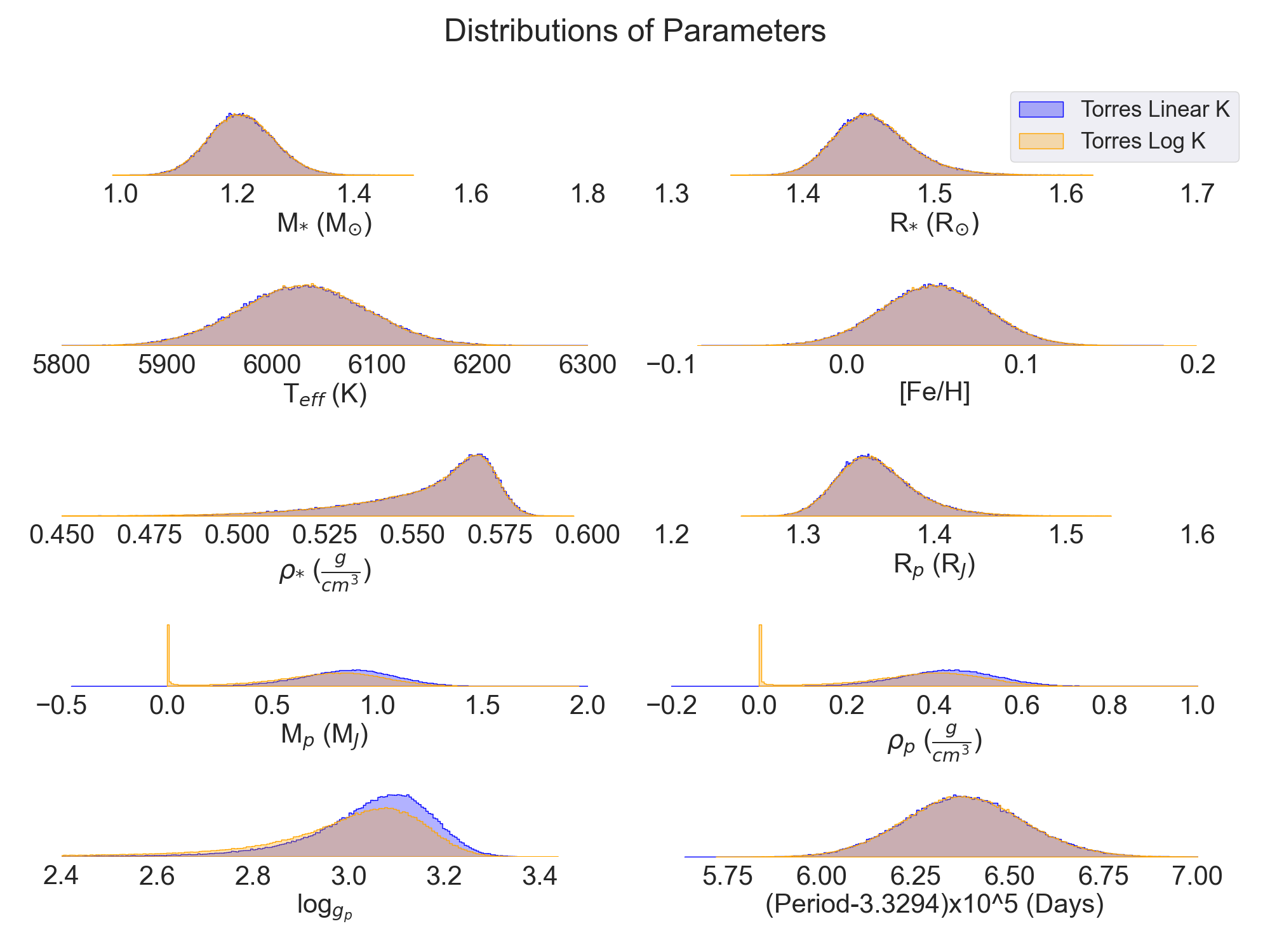
Figure 2: The posterior distributions of the primary direct observables in the KELT-15 system ($P$, $K$, $\delta$, $\tau$, $T_{\rm FWHM}$, and jitter), as well as the derived properties of the host star ($M_{*}$, $R_{*}$), $T_{\rm eff}$, [Fe/H]) and planet($M_{p}$, $R_{p}$, $\log{g_{p}}$). We note that $\rho_{*}$ and $\log{g_{p}}$ can be determined from direct observables. Both models use the Torres relations to break the mass-radius degeneracy, as well as assume a circular orbit. The blue histograms show the posteriors assuming a prior distribution that is uniform in $K$, where as the yellow histograms show the posterior distributions assuming a prior that is uniform in $\log{K}$.

After validating our methodology with the same data set as Rodriguez et al. (2016), we proceed to include TESS observations. We again attempted to model the system in the same way using the Torres relations. In this attempt, we noticed an unusual build up in the posterior probability of $K$ around zero, as shown in the $\log{K}$ distribution shown in Figure 2. The version of MultiFast used and EXOFASTv2 step in $\log{K}$ space by default. This is equivalent to a linear prior in $\log{K}$. This results in a build up around a value of $K$ consistent with zero that was not present in the original analysis. This also introduces build up around zero for other parameters that are derived from $K$, such as planetary mass and density. As we did not include any new radial velocity measurements, and this parameter should not have been affected by the new TESS observations.

However, EXOFASTv2 also provides the option of stepping linearly in $K$. This option did not show the build up in posterior probability at zero, and provided a median value much closer to the value originally published in Rodriguez et al. (2016). This is a somewhat unsettling result as it indicates that a minor change in the method used to step in priors can result in a significantly altered median value of the inferred parameter in the case where $K$ is not extremely well constrained. When stepping in $\log{K}$ we find a median planet mass of $0.76^{+0.25}_{-0.38}M_{J}$. In contrast, when stepping $K$ we find a median of $0.87^{+0.22}_{-0.24}M_{J}$. This is a fractional difference of approximately 13.5% or $0.3\sigma$, assuming the linear $K$ version as the fiducial. Although this is less than a $1\sigma$ change, the difference here is especially concerning since this is the same system, fit with the same radial velocity data and the same method of breaking the mass-radius degeneracy with only a difference in stepping in $K$. This underlines the need for consistent methodology in parameter fitting in order to robustly compare the derived parameters of different exoplanet systems to one another. Of course, the chosen prior in $K$ will have a smaller effect for systems with radial velocity data sets with higher statistical power.

Later updates in October of 2020 to EXOFASTv2 changed from stepping in $\log{K}$ by default to stepping linearly in planet mass. As Figure 3 shows, the results derived from stepping linearly in $K$ and linearly in $M_{p}$ agree extremely well, as expected. This method of stepping in planet mass resolves the build up around $K\sim 0$ and produces a median planet mass of $0.86^{+0.22}_{-0.24}M_{Jupiter}$. For the remainder of this paper, our default method is to step linearly in planet mass.

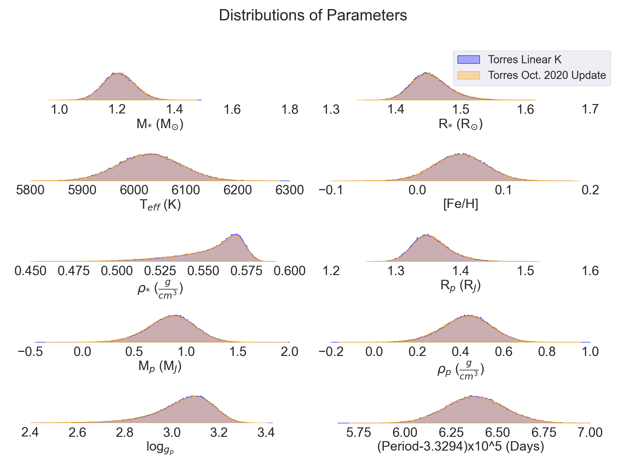
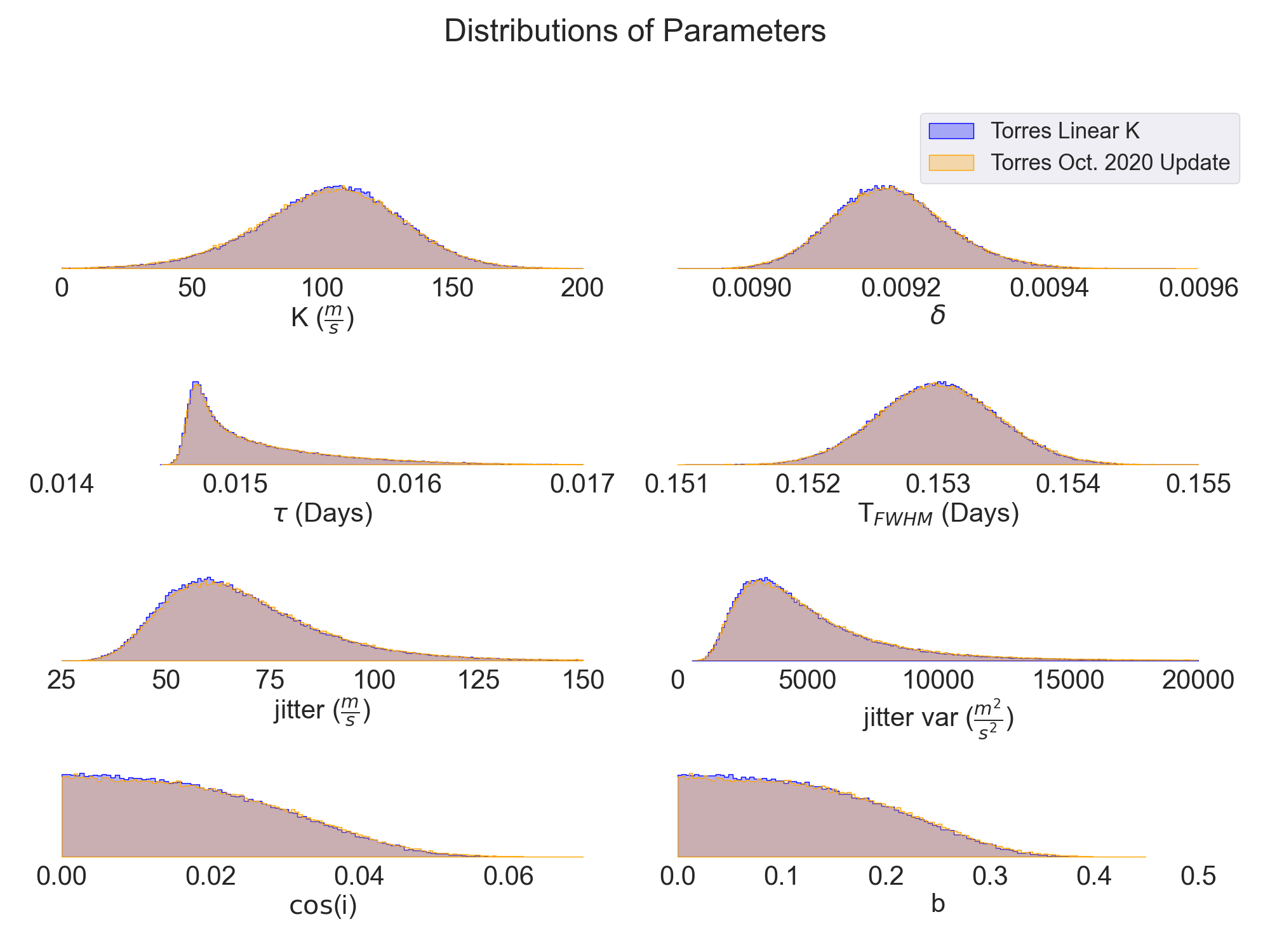
Figure 3: We present the posterior distributions assuming a prior that is uniform in $K$, as well as a prior that is uniform in planet mass, as implemented in the EXOFASTv2 October 2020 update, for the circular Torres analysis for both derived and observable system parameters. We see good agreement between these methods and no longer see the posterior distribution build up around $K\sim 0$.

4 Overview of the Analysis

4.1 Default Model

In this work we consider the ‘default’ model to be one single method of breaking the mass-radius degeneracy and a set of three assumptions. The single methods of breaking the mass-radius degeneracy in the host star encompasses the YY, MIST, Torres, and SED+Gaia. We also include the following three default assumptions:

1. Fixing eccentricity at zero.

2. Applying a prior on the limb darkening coefficients as determined by the Claret tables (Claret & Bloemen (2011) & Claret (2017)).

3. Applying a prior on the stellar effective temperature set by spectroscopic analysis done by Rodriguez et al. (2016).

Therefore, the “default” MIST model uses only the MIST isochrones to break the mass-radius degeneracy and applies all three listed assumptions, whereas the “default” Torres model we would use only the Torres relations and apply the three assumptions. Using more than a single constraint or change in the assumptions is no longer considered a “default” model. Within those assumptions, the inclusion of the Claret (2017) tables and the Agol et al. (2020) transit models are updated versions of those used in Rodriguez et al. (2016) and include band pass information for TESS observations. EXOFASTv2 uses the updated Claret tables to apply a prior on the limb darkening coefficients based on the values determined by the $T_{\rm eff}$, [Fe/H], $\log{g_{*}}$, and a few other characteristics of the host star. This is opposed to fitting the limb darkening coefficients freely. Additionally, since KELT-15b has a period of roughly 3 days, we assume its orbit is nearly circular (Adams & Laughlin, 2006; Goldreich & Soter, 1966). Using equation 3 in Adams & Laughlin (2006), we can roughly expect a circularization timescale of 820 Myr, far shorter than 4.6 Gyr estimated by Rodriguez et al. (2016), which also found KELT-15b to be consistent with a circular orbit within $2\sigma$. However, we also explore the effect of relaxing this assumption on the inferred parameters and their uncertainty. By employing one only method of breaking the mass-radius degeneracy at a time, we can compare each method to the others as they use roughly independent constraints. This also allows us to investigate the results of the constituent parts before multiple methods are applied later in the combination models.

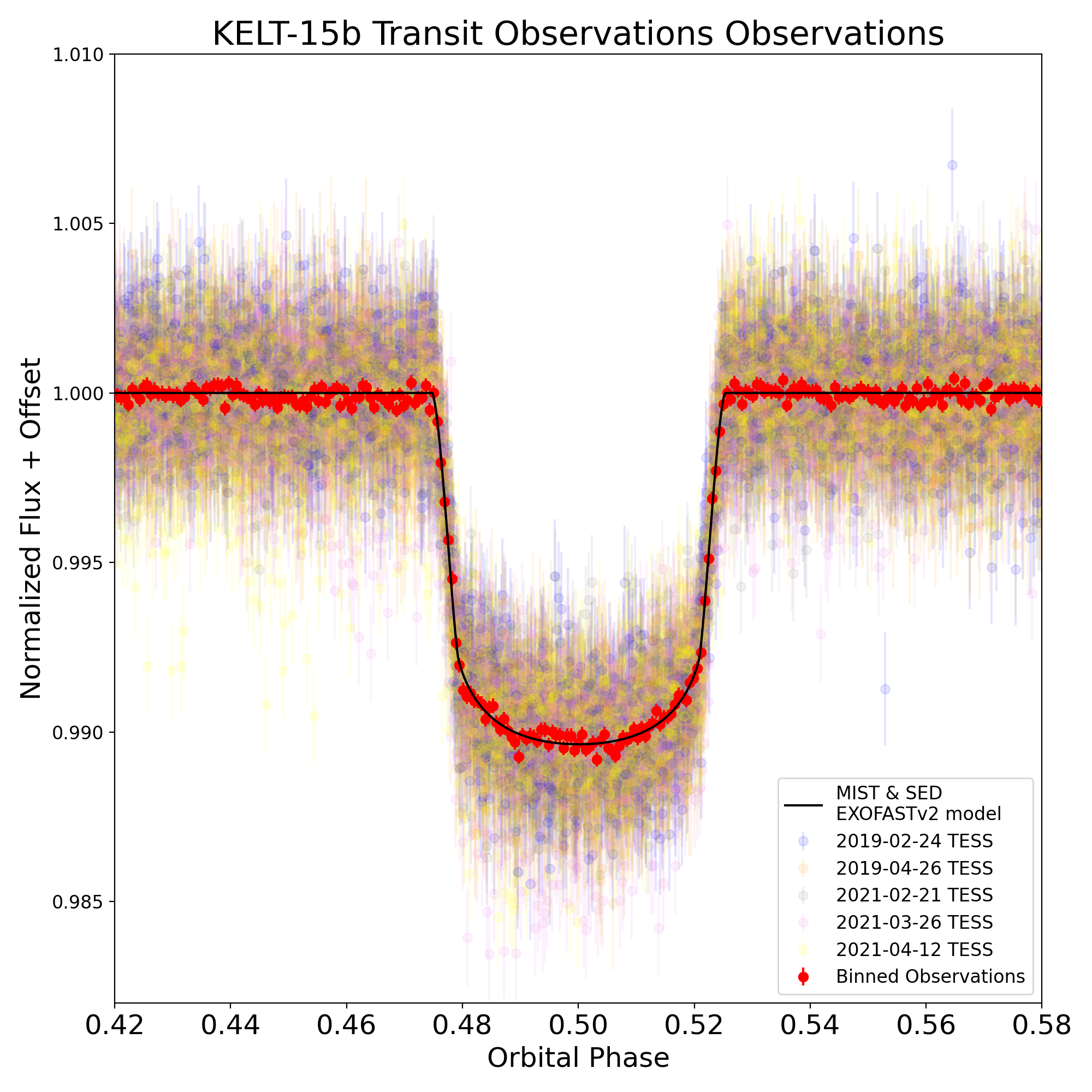
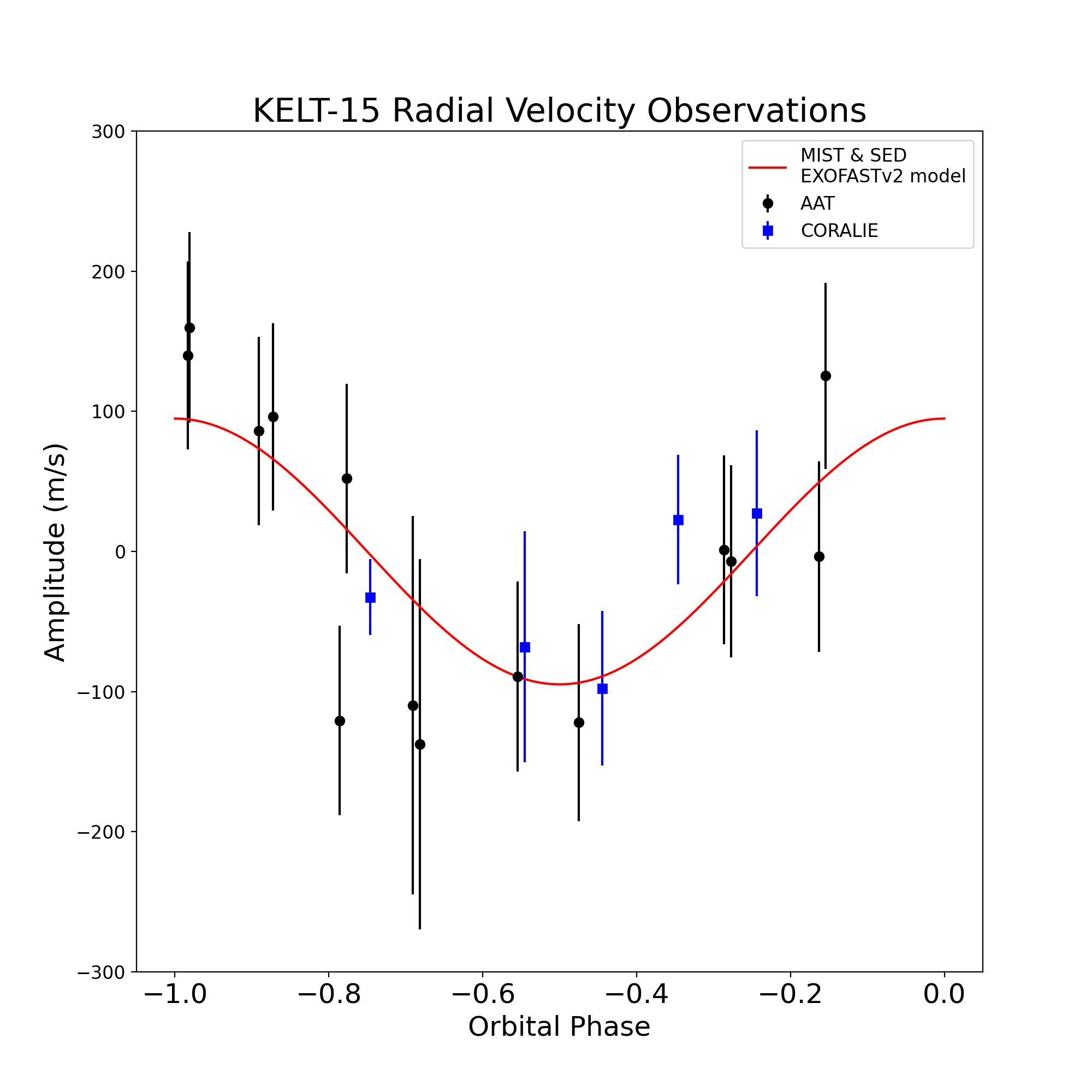
Figure 4: Radial velocity observations used in the original Rodriguez et al. (2016) and the light curves of the TESS observations included in this study. The transit observations on the left and the radial velocity observations on the right are both phase folded. The transit observation compares the data to the EXOFASTv2 model fitting using the MIST isochrones and the SED for the host star characterisation. The associated date represents the start of an observing campaign.

The time series TESS transit observations were downloaded from the Mikulski Archive for Space Telescopes (MAST). We de-trended the SAPFLUX using the wotan package using a transit mask with the published period, and $T_{\rm FWMH}$ and $t_{0}$, the central transit time, estimated by eye (Hippke et al., 2019). This process removes stellar noise and other trends. We ensure that both the transit observations and the radial velocity report their timestamps in $BJD_{TDB}$ (Eastman et al., 2010) and that the radial velocity measurements are reported in m/s as required by EXOFASTv2 . We show the phase folded transit and radial observations used in this study in Figure 4. Once the observations are reduced, we follow a set procedure for each iteration.

1. Use EXOFASTv2 and an SED to fit only the host star

2. Test SED fit of the host star for convergence

3. Use converged stellar fit as starting values for entire system fit, including planet(s). Apply all three default assumptions.

4. Test system fit for convergence. If unconverged, use the median posteriors from the previous fit as starting values for the next fit.

We first use EXOFASTv2 to estimate the radius of the host star. Here we provide priors on $T_{\rm eff}$ and [Fe/H] based on the high-resolution spectra of KELT-15, as described in Rodriguez et al. (2016). We provide a prior on the parallax from Gaia Data Release 2 (Gaia Collaboration et al., 2018, 2016a) with the Stassun & Torres (2018) corrections. We also provide starting values for the stellar radius and mass from Gaia. For this initial stellar only fit we apply only the SED+Gaia degeneracy breaking method.

Second, we test for convergence using the Gelman-Rubin statistic (Brooks & Gelman, 1998). This statistic compares the variance within individual chains to the variance between all of the chains. When the Gelman-Rubin statistic is close to unity, the chains are generally considered well-mixed, whereas values that are much greater than one are an indication that the chains have not converged. We adopt the threshold of a Gelman-Rubin statistic of $<$ 1.01 to indicate convergence, as suggested by EXOFASTv2 (Eastman et al., 2019).

Third, we use the results of the converged SED stellar fit as a starting point for the system global fit using all of the data and priors. This initial SED+Gaia only stellar fit provides starting values for a variety of parameters like stellar radius, mass, distance, equivalent evolutionary point (EEP). We then model the entire system using all detrended transit and radial velocity observations. We begin by applying only one degeneracy breaking method at time. Then, we enable the Claret tables (Claret, 2017) and fix eccentricity at zero. After this set up, we begin the first iteration of this fit. If the fit is not converged we use that iteration to inform the next run by providing starting values for each parameter. We continue to run iterations of the fit using EXOFASTv2 until a Gelman Rubin score of 1.01 is achieved and the fit is considered converged.

4.2 Combining Methods of Stellar Fitting and Variations in Each Model

After the convergence of each “default” model we consider two other configurations: 1) combining methods of breaking the mass-radius degeneracy while maintaining the set of three assumptions and 2) changing our assumptions in both the single and combination constraint models. We are able to combine constraints on our isochrone models, MIST and YY, as well as the semi-empirical Torres relations, with additional constraints from the SED+Gaia method. This is an especially important case as combining constraints from these indirect mass-radius degeneracy breaking methods and the more SED is an increasingly common practice.

The second configuration stems from varying our underlying prior assumptions. We investigate three assumptions: requiring circular orbits, providing a spectroscopically derived prior on $T_{\rm eff}$  and using the Claret models to fit limb darkening coefficients. These models which vary the underlying assumptions are considered “variations.” We only change one assumption and leave the rest to the “default” settings. We apply these assumption changes to all of our single-constraint models (MIST, YY, Torres, SED) and all of our combination constraint models (MIST + SED, YY + SED, and Torres + SED).

For example, while we assume that the orbits of most hot Jupiters are circular ($e=0$), it is important to confirm that the data bears out this assumption. In equation 1, we see that $e$ is covariant with $K$, the semi-amplitude in radial velocity observations. Eccentricity plays an important role in estimating the mass of the planet which depends on accurate values of $K$. From equations 3 and 4, we also know that eccentricity plays an important role in constraining the density of the host star. Thus, we also adopt runs for each single and combination mass-radius degeneracy breaking method that allows eccentricity to be a free parameter to investigate the impacts on $\rho_{*}$ and other system parameters. In these cases, we maintain the other two assumptions of a complete prior with an associated uncertainty on the value of $T_{\rm eff}$, and applying the Claret tables to determine the limb darkening coefficients. Thus we can investigate the result of only changing the eccentricity from fixed at zero to being a freely fit parameter. By doing this for each single and combination method of breaking the mass-radius degeneracy, we can see if different fitting degeneracy breaking methods respond differently to fitting the eccentricity of the planet freely.

Correspondingly, we test a separate case that allows free fitting of the limb darkening coefficients instead of using priors based on the Claret tables (Claret, 2017; Claret & Bloemen, 2011). This case still maintains the assumptions of a circular orbit, and a prior on $T_{\rm eff}$. The Claret tables of limb darkening values are used to calculate the change in surface brightness from the center of a star to its limb. The Claret tables use band-pass wavelengths and a grid of $T_{\rm eff}$, $\log{g_{*}}$, and [Fe/H] all estimated from stellar atmosphere models like PHOENIX (Witte et al., 2009; Husser et al., 2013) and ATLAS (Claret & Bloemen, 2011). EXOFASTv2 then places a prior on the limb darkening coefficients based on the Claret table value that most closely matches the $T_{\rm eff}$, $\log{g_{*}}$, and [Fe/H] for the host star at each step when the Claret tables are employed. Here, we investigate a case where we do not apply the constraints of the Claret table and fit the limb darkening coefficients as free parameters, not tied to the estimate of $T_{\rm eff}$ or metallicity.

Finally, we test a case where we do not adopt the spectroscopically-derived prior on $T_{\rm eff}$. In this case, the only direct constraint in $T_{\rm eff}$ comes from the SED, in those cases where this information is included. In several of these variations, we reduce the amount of information constraining these systems. As a result, the fits converge significantly more slowly. In these cases, we adopt a convergence threshold for the Gelman-Rubin statistic of 1.1 for the variation models. For these fits, we have performed limited experiments where we require a GR statistic of 1.01 and find that adopting the less conservative threshold has no qualitative effect on our conclusions.

5 Results

5.1 Results of Default Model

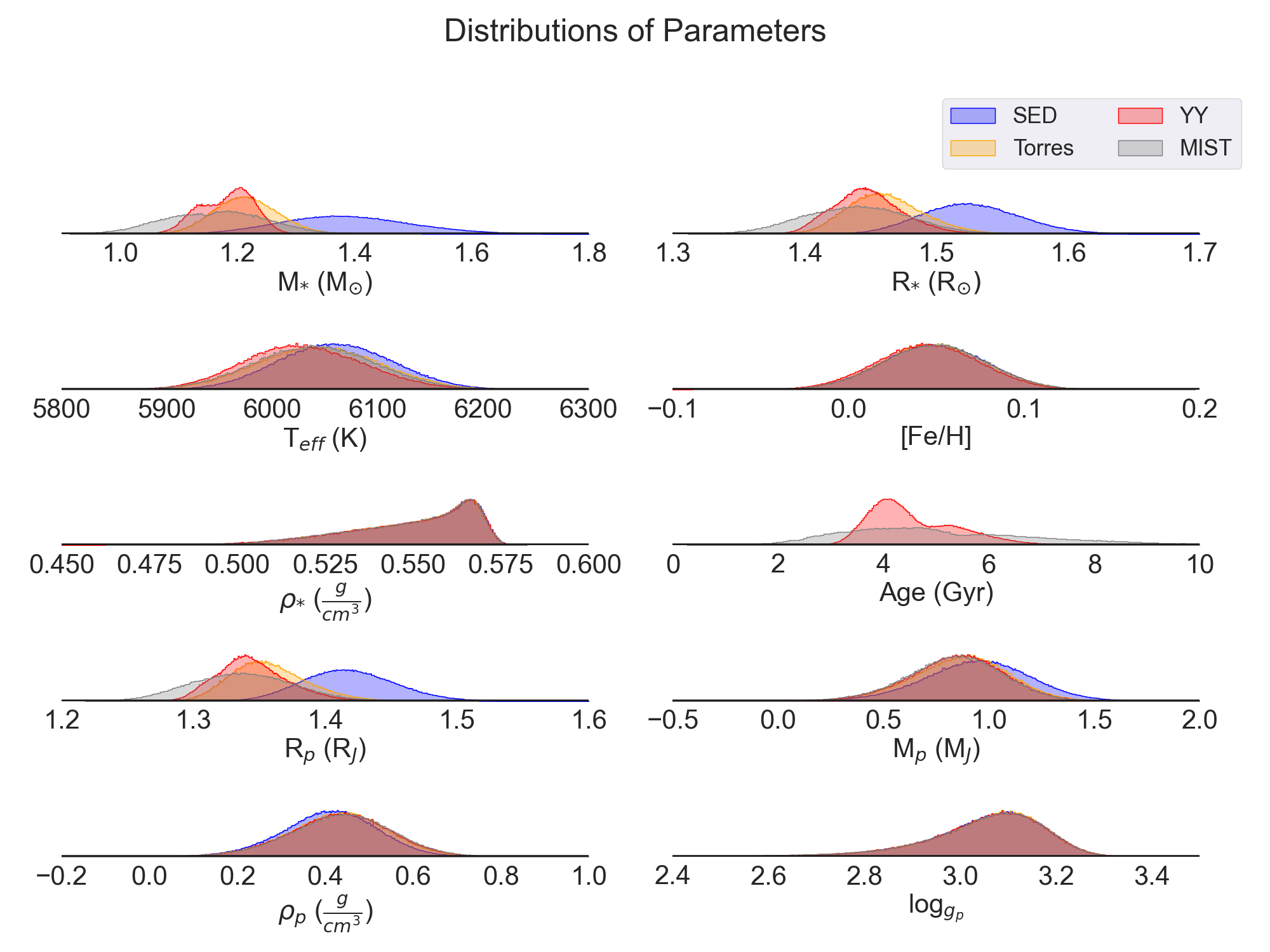
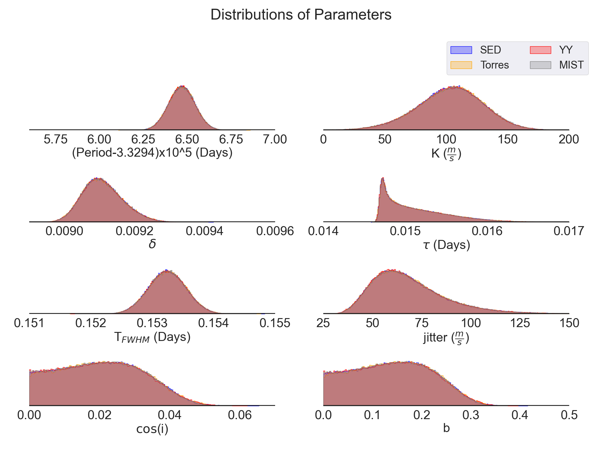
Figure 5: Posterior distributions of our “default” models: Torres, YY, MIST, and SED. We assume circular orbits, include a prior on $T_{\rm eff}$ from high-resolution spectroscopy, and use the Claret limb darkening tables (Claret, 2017). The Torres and SED constraints do not provide stellar Age information and are not shown in that panel.

Figure 5 shows the posterior distributions for several system parameters for all four single-constraint models (Torres, YY, SED, MIST). The shaded regions in this figure represent histograms of the posterior distributions for each parameter for each model. We see that all four single-constraint models (Torres, YY, SED, MIST) roughly agree with each other regarding the directly observable parameters ($P$, $K$, $\delta$, $\tau$, eccentricity, $\log{g_{p}}$, etc.). On the other hand, there are noticeable differences in medians and uncertainties for the derived parameters ($M_{*}$, $R_{*}$, Stellar Age, $R_{p}$, $M_{p}$, etc.). The median values and uncertainties of the observational properties shown in the lower half of the figure demonstrate similar posterior distributions across all stellar constraint models. When compared to the original discovery paper, we find a significant decrease in the uncertainty in the period by 50%, due to the inclusion of TESS observations which provide a longer baseline. We find smaller uncertainties for the radius of the planet corresponding to a fractional difference in the uncertainties of 65% between the YY implementation in Rodriguez et al. (2016) and the YY version of this work. This is directly related to a 62% decrease in the fractional uncertainty in the stellar radius due to the additional photometric transit observations. In particular, TESS observations provide more information on the density of the host star and the transit depth with fractional improvements of 84% and 87% in the uncertainties of these parameters, respectively. The values for select parameters are presented in Table 3. Our complete suite of parameters for the single constraint default fits are shown in Tables 5 and 6.

All of the single constraint mass radius degeneracy breaking methods we consider, including the Rodriguez et al. (2016) fits, result in a consistent stellar density. This is not surprising, as the inferred stellar density is essentially empirically constrained. In the case of these single constraint models, we can characterize the density of the host star through our priors on the $T_{\rm eff}$, [Fe/H], and constraints from the light curve. For example, the Torres semi-empirical relations are equations for $\rm M_{*}$ and $\rm R_{*}$ as a function of $T_{\rm eff}$, [Fe/H], and $\log g_{*}$. These relations can be rewritten to be a function of $T_{\rm eff}$, [Fe/H], and $\rho_{*}$ (Enoch et al., 2010). From equation 4, we can estimate ${\rho_{*}}$ directly from the light curve. Thus, we can solve for $M_{*}$ and $R_{*}$. Similarly, the evolutionary track methods (MIST, YY) provide relationships for $M_{*}$ and $R_{*}$ in terms of $T_{\rm eff}$, [Fe/H], and stellar age. Here evolutionary age serves as the free parameter. The SED method again uses the priors on $T_{\rm eff}$and [Fe/H], but adds a constraint on $R_{*}$. However the SED itself can not constrain $M_{*}$, making it a free parameter. In all four of these instances the constraint on ${\rho_{*}}$ from the light curve is needed to maked independent measurements of $M_{*}$ and $R_{*}$, and thus a complete solution to the system. Since the priors on $T_{\rm eff}$, [Fe/H] are the same in all the ‘default’ single constraint models, and the only constraint on $\rho_{*}$ comes from the light curve, we expect agreement in stellar density across the single constraint models, as observed. The rest of the empirically-constrained parameters (e.g. $\delta$, $\tau$, $T_{FWHM}$) are also in good agreement, because, as with $\rho_{*}$, the only constraint on these parameters is through the light curve. This ignores the dependence of the prior of limb darkening coefficients on $T_{\rm eff}$and $\log{g_{*}}$. These effects are weak, the limb darkening parameters do not strongly depend on $T_{\rm eff}$and $\log{g_{*}}$.

We do not see the same uniformity in the derived parameters. In particular, the YY isochrones produce a bimodal distribution in the mass of the host star. This bi-modality has been observed in other transiting planet systems, and is a result of the fact that, for fixed values of the observable parameters, the host star can be on the main-sequence or sub-giant branch of its evolution, with different masses for each scenario. We see a corresponding bi-modality in the derived age of the system. The taller peak of the bimodal distribution in mass seems to agree well with the peak of the Torres distribution. Meanwhile the shorter peak in the mass distribution aligns more closely with the spread of the MIST distribution. For $R_{*}$, YY provides a median value that is smaller than the Torres and SED-only models and slightly larger than the MIST-only model. The medians of the posterior distribution for the planetary radius are essentially directly proportional to the medians of the stellar radius, as the transit depth $\delta$ is very tightly constrained by the TESS data.

Most notably, we show that MIST consistently produces the smallest values for $M_{*}$ and $R_{*}$ as well as $M_{p}$ and $R_{p}$. Conversely, the SED model consistently produces the largest values for these parameters. An applied prior to $T_{\rm eff}$ and [Fe/H] consistently kept these two values clustered. The MIST distribution also shows a less noticeable but still prominent bi-modality in the $M_{*}$ and stellar age.

Table 3: Selected Parameter values for KELT-15b

Parameters	MIST	YY	SED	Torres	Torres (No TESS)	Units
$M_{*}$	$1.165^{+0.086}_{-0.093}$	$1.187^{+0.041}_{-0.056}$	$1.38^{+0.12}_{-0.11}$	$1.213^{+0.057}_{-0.053}$	$1.208^{+0.056}_{-0.054}$	M⊙
$R_{*}$	$1.44^{+0.041}_{-0.042}$	$1.447^{+0.028}_{-0.025}$	$1.525^{+0.04}_{-0.036}$	$1.46^{+0.031}_{-0.027}$	$1.452^{+0.031}_{-0.026}$	R⊙
$\rho_{*}$	$0.553^{+0.013}_{-0.025}$	$0.553^{+0.014}_{-0.025}$	$0.553^{+0.014}_{-0.025}$	$0.553^{+0.014}_{-0.025}$	$0.56^{+0.011}_{-0.026}$	$\frac{g}{cm^{3}}$
$T_{eff}$	$6039^{+59}_{-59}$	$6028^{+60}_{-55}$	$6059^{+56}_{-55}$	$6043^{+60}_{-59}$	$6029^{+61}_{-60}$	K
$[F/H]$	$0.049^{+0.03}_{-0.03}$	$0.045^{+0.03}_{-0.03}$	$0.049^{+0.03}_{-0.03}$	$0.048^{+0.03}_{-0.03}$	$0.049^{+0.03}_{-0.03}$	-
$\rho_{p}$	$0.44^{+0.11}_{-0.12}$	$0.43^{+0.11}_{-0.12}$	$0.41^{+0.11}_{-0.11}$	$0.43^{+0.11}_{-0.12}$	$0.43^{+0.11}_{-0.12}$	$\frac{g}{cm^{3}}$
$R_{p}$	$1.337^{+0.04}_{-0.039}$	$1.343^{+0.03}_{-0.024}$	$1.417^{+0.037}_{-0.034}$	$1.355^{+0.032}_{-0.026}$	$1.354^{+0.032}_{-0.025}$	RJ
$M_{p}$	$0.84^{+0.22}_{-0.24}$	$0.85^{+0.22}_{-0.23}$	$0.95^{+0.25}_{-0.26}$	$0.87^{+0.22}_{-0.24}$	$0.86^{+0.22}_{-0.24}$	MJ
Period	$3.32946^{+7.6e-07}_{-7.6e-07}$	$3.32946^{+7.5e-07}_{-7.5e-07}$	$3.32946^{+7.6e-07}_{-7.6e-07}$	$3.32946^{+7.6e-07}_{-7.5e-07}$	$3.32946^{+1.6e-06}_{-1.6e-06}$	Days
b	$0.14^{+0.086}_{-0.091}$	$0.14^{+0.086}_{-0.091}$	$0.141^{+0.086}_{-0.091}$	$0.141^{+0.085}_{-0.09}$	$0.117^{+0.1}_{-0.081}$	-
$log(g_{p})$	$3.068^{+0.099}_{-0.14}$	$3.068^{+0.099}_{-0.14}$	$3.068^{+0.098}_{-0.14}$	$3.069^{+0.096}_{-0.14}$	$3.065^{+0.1}_{-0.14}$	-
K	$103^{+26}_{-29}$	$103^{+26}_{-29}$	$103^{+26}_{-28}$	$104^{+26}_{-29}$	$103^{+26}_{-29}$	$\frac{m}{s}$
$\delta$	$0.009105^{+6.3e-05}_{-5.3e-05}$	$0.009105^{+6.3e-05}_{-5.3e-05}$	$0.009105^{+6.4e-05}_{-5.3e-05}$	$0.009104^{+6.4e-05}_{-5.3e-05}$	$0.009184^{+8e-05}_{-7.4e-05}$	-
$\tau$	$0.01502^{+0.00054}_{-0.00027}$	$0.01502^{+0.00054}_{-0.00028}$	$0.01502^{+0.00054}_{-0.00028}$	$0.01502^{+0.00054}_{-0.00028}$	$0.01496^{+0.00056}_{-0.0002}$	Days
$T_{fwhm}$	$0.15325^{+0.00031}_{-0.00031}$	$0.15324^{+0.00031}_{-0.00031}$	$0.15324^{+0.00031}_{-0.00031}$	$0.15325^{+0.00031}_{-0.00031}$	$0.153^{+0.00047}_{-0.00046}$	Days
$cos(i)$	$0.02^{+0.013}_{-0.013}$	$0.02^{+0.013}_{-0.013}$	$0.02^{+0.013}_{-0.013}$	$0.021^{+0.013}_{-0.013}$	$0.017^{+0.015}_{-0.012}$	-
jitter	$65^{+22}_{-15}$	$65^{+22}_{-15}$	$65^{+22}_{-15}$	$65^{+22}_{-15}$	$66^{+22}_{-15}$	$\frac{m}{s}$

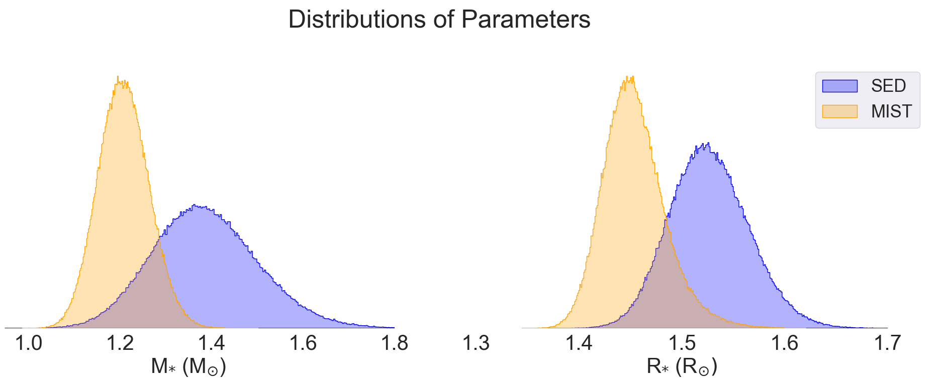
Figure 6: Comparison between posterior distributions for the MIST isochrones and SED fit for stellar mass and stellar radius.

The differences in $M_{*}$ and $R_{*}$ lead directly to differences in the planet radius and mass. We highlight the distributions for stellar mass and radius derived from the MIST evolutionary tracks and the SED method in Figure 6. We see a fractional difference between the MIST and SED models of 5.9% or 2.0 times the difference in the medians divided by the larger uncertainty ($\sigma$). The stellar radius estimated by the MIST isochrones is $1.440^{+0.041}_{-0.042}R_{\odot}$ and the SED is $1.525^{+0.040}_{-0.036}R_{\odot}$. In planetary radius, this directly leads to a similar 6.0% fractional difference or $2.0\sigma$ where the MIST isochrones estimate is $1.337^{+0.040}_{-0.039}R_{J}$ and the SED estimate is $1.417^{+0.037}_{-0.034}R_{J}$. The uncertainty introduced by changing the method of breaking the stellar mass-radius degeneracy is roughly twice as large as the statistical uncertainty in planetary radius. The stellar mass shows the largest difference between the two models. The MIST isochrones estimated a much smaller mass of $1.165^{+0.086}_{-0.093}M_{\odot}$ compared to the $1.38^{+0.12}_{-0.11}M_{\odot}$ of the SED fit. This is a fractional difference in stellar mass of 18.5%, compared to the MIST model, where the statistical uncertainties reside at the 7% level. In planetary mass, we see a similar fractional difference of 13.1% compared to the MIST estimate. However the planetary masses have much larger uncertainties making this difference only $0.4\sigma$. Except for the values produced by the SED, the planet mass is centrally clustered around a single value due to the large uncertainty in the semi-amplitude of the radial velocity observations. Generally, these wider uncertainties buffer planetary mass estimates from the effects of changing stellar models. We expect that the choice of the method to break the mass-radius degeneracy will have a more pronounced effect on the planetary mass if more frequent and higher precision radial velocity observations are collected.

The directly observed parameters like $T_{\rm FWHM}$, $\delta$, $\rho_{*}$, and RV jitter are largely consistent across all models. Since all models are using the same observations, this is confirmation of our method and ensures that the only changes seen in other parameters derive solely from the different methods of breaking the mass-radius degeneracy. We show that the directly observable parameters are insulated from any effect of changing the stellar modeling method used in our “default” method. As we will see in the next section, however, when we combine different methods of breaking the mass-radius degeneracy, we find that the posterior distributions of the observable parameters are slightly different.

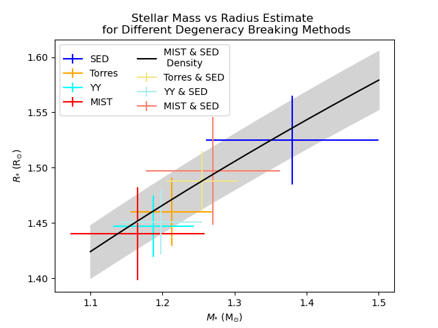
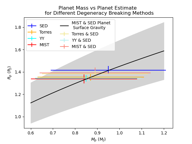
Figure 7: Mass and Radius estimates for the default and combined models with their associated uncertainties for the host star in the left panel and the planet KELT-15b in the right panel. They are compared to the respective MIST + SED density estimate. The gray region shows the uncertainty on the MIST + SED density

5.2 Results of Combining Methods of Stellar Fitting

We also compare the results of combining two methods of breaking the mass-radius degeneracy together. We investigate combining the YY isochrones and the SED methods, MIST isochrones and the SED, and finally the Torres relations with the SED. We find significant differences between the single-constraint methods and these combined methods.

The results of the application of these combinations of methods are shown in Figure 8. Here we see that MIST + SED produces the largest stellar mass and radii, while YY + SED produce the smallest values. The Torres + SED combination model, the most empirical of the three, produce values that fall squarely between the other two. We also see a similar spread in effective temperature for the host star. The information on this parameter comes directly from the spectroscopically-derived prior, the SED, and indirectly through the stellar evolutionary models and limb darkening. We see that the MIST + SED estimate produces the largest effective temperature, which contributes to this model also producing the largest stellar mass and radius estimates. We also see that YY + SED produces the smallest effective temperature. The fractional difference in host star radius between the larger MIST + SED stellar radius and the lower YY + SED estimate is about 3% or $1\sigma$, which is the same magnitude as the statistical uncertainty. The full results of these combined methods are presented in Tables 13 and 14.

We see a corresponding difference in the derived planet radius of 3.2% or $1\sigma$ between the MIST + SED radius compared to the YY + SED radius. This indicates a significant spread between two models that are both using additional color magnitude information. Based on our level of convergence, repetitions of the same model on the same observations should produce agreement at the level $0.05\sigma$ (see Section 23.4 of Eastman et al. 2019). Changes of $\sim 1\sigma$ indicate clear differences in the medians produced by these two methods. YY produces the tightest bound on the stellar radius and density. We also see differences of $0.6\sigma$ in stellar density. Notably we also see a small difference of 0.32% ($0.4\sigma$) in the transit depth $\delta$, a quantity that should be a pure observable.

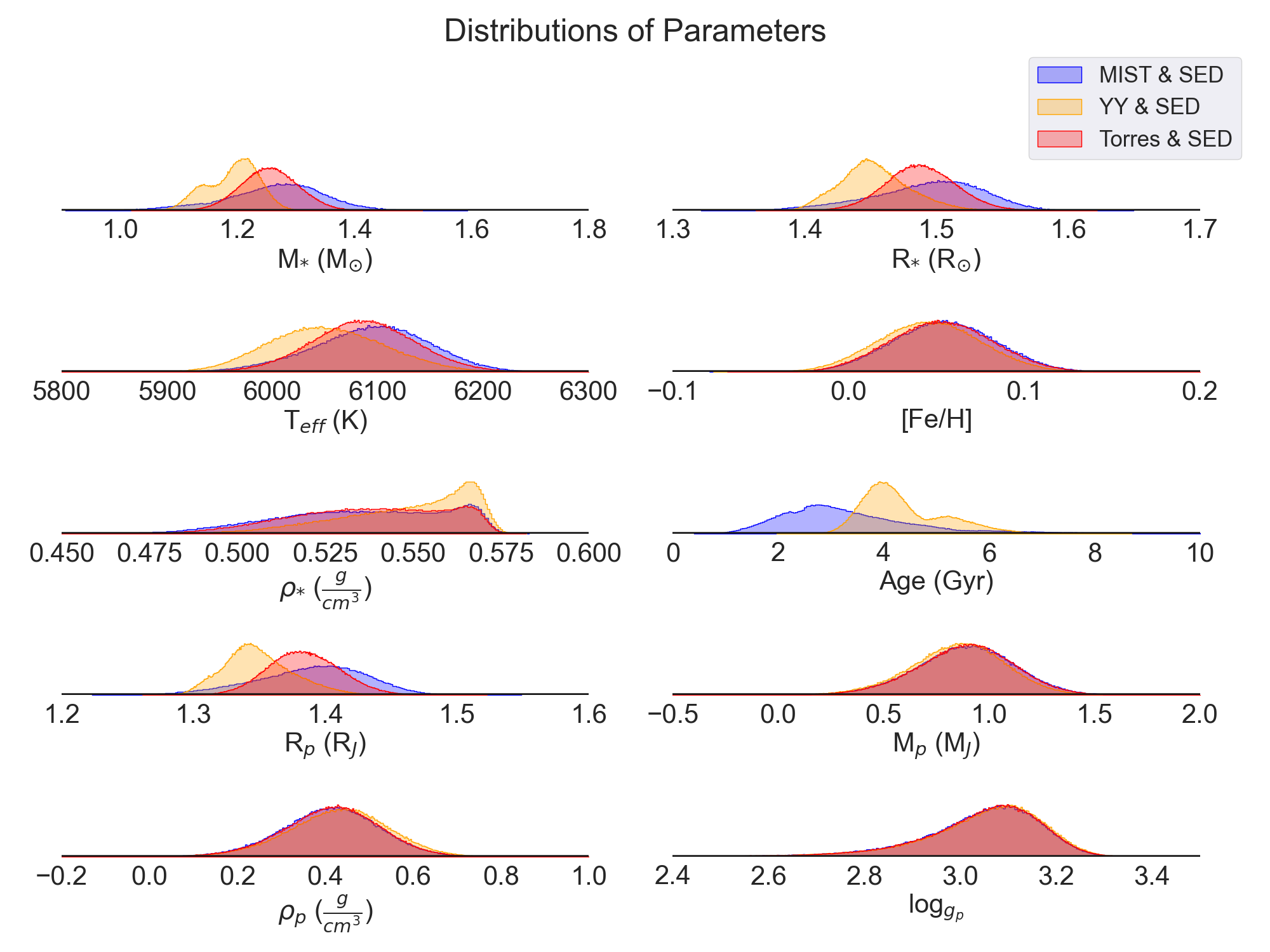
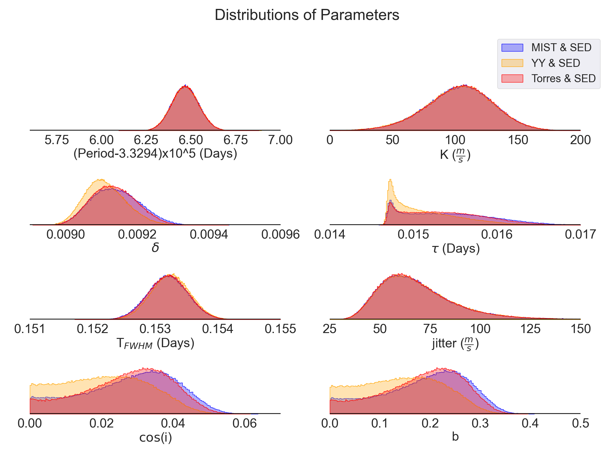
Figure 8: Results of our combined models: Torres + SED, YY + SED, MIST + SED, We assume circular orbits, provide effective temperature priors, and use the Claret limb darkening tables (Claret, 2017). The Torres + SED constraint does not provide stellar Age information and is not shown in that panel.

Table 4: Selected Parameter values for the Combined Constraint fits of KELT-15b

Parameters	MIST + SED	YY + SED	Torres + SED	Units
$M_{*}$	$1.27^{+0.074}_{-0.093}$	$1.198^{+0.037}_{-0.057}$	$1.255^{+0.05}_{-0.049}$	M⊙
$R_{*}$	$1.497^{+0.038}_{-0.049}$	$1.451^{+0.029}_{-0.024}$	$1.488^{+0.027}_{-0.026}$	R⊙
$\rho_{*}$	$0.537^{+0.025}_{-0.027}$	$0.552^{+0.014}_{-0.025}$	$0.539^{+0.023}_{-0.025}$	$\frac{g}{cm^{3}}$
$T_{eff}$	$6095^{+54}_{-59}$	$6050^{+59}_{-54}$	$6085^{+50}_{-50}$	K
$[F/H]$	$0.054^{+0.03}_{-0.03}$	$0.046^{+0.03}_{-0.03}$	$0.053^{+0.03}_{-0.03}$	-
$\rho_{p}$	$0.41^{+0.11}_{-0.11}$	$0.43^{+0.11}_{-0.12}$	$0.42^{+0.11}_{-0.11}$	$\frac{g}{cm^{3}}$
$R_{p}$	$1.392^{+0.039}_{-0.048}$	$1.347^{+0.03}_{-0.023}$	$1.383^{+0.029}_{-0.027}$	RJ
$M_{p}$	$0.89^{+0.23}_{-0.25}$	$0.86^{+0.22}_{-0.24}$	$0.89^{+0.22}_{-0.24}$	MJ
Period	$3.3294647^{+7.7e-07}_{-7.5e-07}$	$3.3294647^{+7.7e-07}_{-7.6e-07}$	$3.3294647^{+7.7e-07}_{-7.5e-07}$	Days
b	$0.2^{+0.073}_{-0.11}$	$0.144^{+0.086}_{-0.094}$	$0.194^{+0.069}_{-0.1}$	-
$log(g_{p})$	$3.06^{+0.098}_{-0.14}$	$3.067^{+0.097}_{-0.14}$	$3.063^{+0.097}_{-0.14}$	-
K	$104^{+26}_{-28}$	$103^{+26}_{-29}$	$104^{+26}_{-28}$	$\frac{m}{s}$
$\delta$	$0.009136^{+7.3e-05}_{-6.6e-05}$	$0.009107^{+6.4e-05}_{-5.3e-05}$	$0.009132^{+6.8e-05}_{-6.2e-05}$	-
$\tau$	$0.01537^{+0.00062}_{-0.00054}$	$0.01504^{+0.00055}_{-0.00029}$	$0.01533^{+0.00056}_{-0.00048}$	Days
$T_{fwhm}$	$0.1532^{+0.00032}_{-0.00032}$	$0.15324^{+0.00031}_{-0.00031}$	$0.15321^{+0.00032}_{-0.00032}$	Days
$cos(i)$	$0.029^{+0.011}_{-0.017}$	$0.021^{+0.013}_{-0.014}$	$0.029^{+0.011}_{-0.015}$	-
jitter	$65^{+22}_{-15}$	$65^{+22}_{-15}$	$65^{+22}_{-14}$	$\frac{m}{s}$

To compare these combined methods with the “default” single-constraint methods, we show the mass and radius estimates in Figure 7 for both the planet and the host star. We also show the stellar density $\rho_{*}$ as estimated by the MIST + SED iteration with the black line with the $1\sigma$ uncertainty shown as the grey band. We see that all of our mass and radius estimates yield the same $\rho_{*}$ to within $1\sigma$, as expected given that $\rho_{*}$ is nearly a direct observable and therefore approximately the same for all fits. We again see that the SED alone method produces the largest values for both radius and mass. MIST alone provides the smallest estimates and the MIST + SED iteration is located between these two. Unsurprisingly, these two continue to serve as bookends even when the combination models are introduced. The YY and YY + SED models are the most similar of any of the single and double constraint pairs. All of the planet density estimates are extremely consistent with the MIST + SED estimate, primarily due to the large uncertainties in planet mass due to the limited radial velocity observations. It is also comforting that the MIST + SED mass and radius estimates are aligned with the MIST + SED density.

5.3 Results of Variation in Each Model

In our reanalysis of KELT-15b we use four different single constraint methods to break the degeneracy between planetary mass and radius. These methods are SED+Gaia, Torres, YY isochrones, MIST isochrones. We also investigate a combination of the indirect methods in conjunction with the SED. As shown in earlier figures each method provides characteristically different results in several derived parameters. Using MIST isochrones alone provide our smallest stellar radii and SEDs alone produce our largest stellar radii. The other three methods, and combinations fall in-between.

However, the choice of model is not the only component that plays a demonstrable role in estimating planetary system parameters. We additionally test effects of the three assumptions: 1) requiring a circular orbit, 2) using the Claret Tables a priors on the limb darkening coefficients, and 3) adopting a spectroscopically-derived prior on the $T_{\rm eff}$. Each of these assumptions play a different role in characterising the exoplanet system. Eccentricity has a well defined role in estimating the mass of the planet as shown in equation 1, so we consider a case where it is fit freely. Allowing the eccentricity to be free also loosens the relation between the light curve observables and $\rho_{*}$ (see. Eqns. 3 and 4). The use of the Claret limb darkening tables (Claret, 2017) as a prior on the limb darkening parameters, which depends on model parameters like $T_{\rm eff}$ and $\log(\rm g_{*})$, affects the determination of the “directly” observed parameters. Therefore, we consider models where the limb darkening coefficients are fit freely. Finally, we explore the impact on our posteriors when we drop the spectroscopically-derived prior on $T_{\rm eff}$. Each of these three assumptions are the basis for a “variation” where we alter one of these assumptions and keep the others in line with our “default” models. For example, to explore the effects of eccentricity, we conduct an iteration where we apply the Claret tables, provide the spectroscopically derived $T_{\rm eff}$ prior, but allow eccentricity to vary freely. The results for the eccentricity variation for the single constraint models are shown in Tables 7 and 8. The eccentric combination constraint models are presented in Tables 15 and 14.

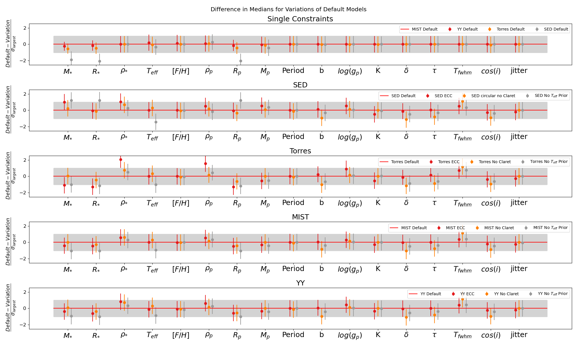
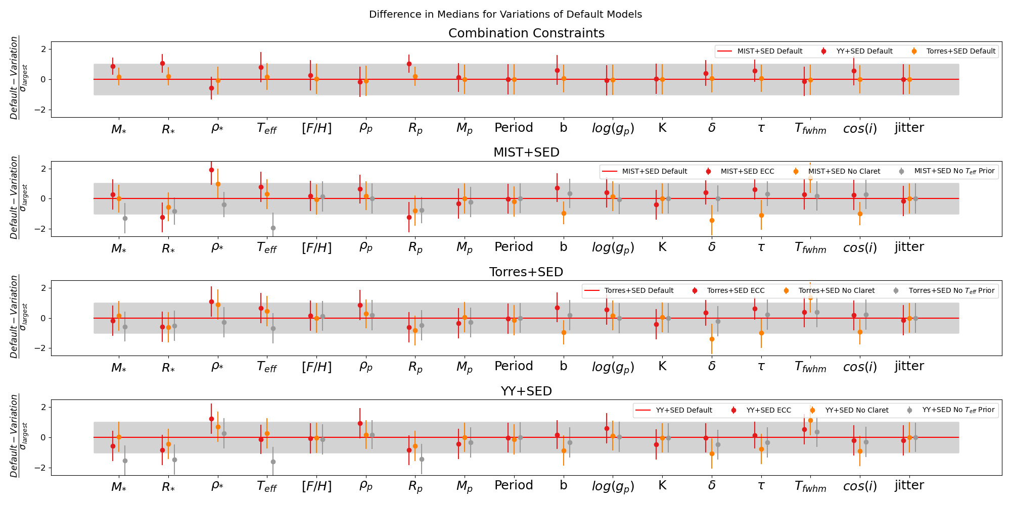
Figure 9: Here we show the difference in medians of the variations compared to the “default” model represented by the red line. We take the difference of the two models and divide by the larger uncertainty to find the $\sigma$ difference represented here. The grey bar represents a $1\sigma$ difference.

We compare the results for each variation of the “default” models and combination models. Our results are represented in figure 9. We show the difference between the “default” model median for each parameter and the “variation” model median with that difference divided by the larger uncertainty in the two models or $(\rm Default-\rm Variation)/\sigma_{largest}$. Here $\sigma_{largest}$ is the larger of the uncertainty in the default model or the uncertainty in the variation. The gray bar represents a difference of $1\sigma_{largest}$ from the default model. For example, in the SED default model and its variations we see that many of the directly observed parameters fall within the $1\sigma$ region. However, many of the derived parameters like mass, radius, effective temperature, and density of the host star vary by more than $1\sigma$ when different variations are applied. As a result we also see variation in the derived radius of the planet based on these different model constraints. The choice of whether to fix $e=0$ or to let it be a free parameter has a particularly large effect on the median value and uncertainty in the stellar density, as expected given by equations 3 and 4. This then propagates to other inferred parameters, such as $R_{*}$ and by extension $R_{p}$. For the combination models, when including the information from the SED+Gaia parallax, the stellar radius is more tightly constrained. Thus, the additional uncertainty introduced by allowing for a free eccentricity is somewhat ameliorated. We also observe a significant increase in the uncertainty in $T_{\rm eff}$ when the prior was removed. This is the logical conclusion of using less information by removing the prior but we see this also has effects on $M_{*}$ and $R_{*}$, producing values that are outside of the $1\sigma$ range.

We see that the Torres single-constraint models are particularly sensitive to allowing the planet eccentricity to vary freely and on using a prior for stellar temperature. The Torres single-constraint model is rather insensitive to whether or not we apply a prior on the limb darkening using the Claret tables. The strong dependence on the $T_{\rm eff}$ prior and dramatic increase in uncertainty, by a rough factor of 18, is not surprising since the Torres relations alone do not supply additional constraints on stellar temperature in any way. Thus the Torres single-constraint models with a $T_{\rm eff}$ prior only constrain $T_{\rm eff}$ indirectly, though the relations themselves and the constraint on $\rho_{*}$ through the light curve observables. The results of not supplying a prior on the effective temperature result in an approximately $1\sigma$ difference from the default model due to the large uncertainties in $T_{\rm eff}$. The uncertainties on the stellar mass and radius also dramatically increase by factors of roughly 5. Additionally, we see large differences from the default baseline when eccentricity was allowed to vary freely and was not fixed at zero. The largest changes, and increase to uncertainty, caused by free eccentricity compared to the default model occur in $\rm R_{*}$ and $\rm R_{p}$ as well as $\rm\rho_{*}$. Equations 4 and 3 show the dependence of stellar density on eccentricity, contributing to the roughly 50% or $2\sigma$ change in $\rho_{*}$, a parameter rather resistant to the other variations. The uncertainty in $\rho_{*}$ is 7 times the default model uncertainty. This change in the estimate of the $\rho_{*}$ and the relatively stable mass estimate then contribute to the change in $R_{*}$ of $1.3\sigma$ or 31% with uncertainties 12 times greater than the default model. This change in stellar radius then has direct follow-on effects for the planetary radius where we see a similar difference of $1.3\sigma$ or 31%.

In general, we find that the fits using MIST constraints were more robust against our variations. We still do observe differences in stellar radius and density, as well as the planet radius when the eccentricity is varied or the $T_{\rm eff}$prior is removed. However these differences are less than $\sim 1\sigma$. The variation models produce inflated uncertainties such that the default version of the MIST model is consistent within $1\sigma_{variation}$. One of the largest changes came from the $T_{\rm eff}$ estimate when no prior on $T_{\rm eff}$ was adopted. This produced an approximately $0.9\sigma$ difference in the medians an a factor of 9 inflation in the uncertainty. Removing the stellar temperature prior also impacted the estimated $\rm M_{*}$, by 19% or $\sim 1\sigma$, and $\rm R_{*}$, by 6.5% or $\sim 1\sigma$. However, introducing free eccentricity increased the uncertainty of $\rho_{*}$ and produced a difference of 18.6% or $0.6\sigma$. In the eccentric case we see changes of $\sim 0.4\sigma$ in both $\rm M_{*}$ and $\rm R_{*}$.

The YY models stayed almost entirely within $1-\sigma$ differences for the variation model that did not use the Claret tables to fit the limb darkening coefficients, but did display some significant increases in uncertainty with free eccentricity and the starting temperature variations. For the no Claret models many of the parameters changed by less than the $1\sigma$ range, with the exceptions of transit duration and transit depth, although these two parameters fall just outside the $1\sigma$ window. Variations in eccentricity and starting temperature provide larger effects on $M_{*}$, $R_{*}$, $T_{\rm eff}$, and $R_{p}$. In the case of no prior on $T_{\rm eff}$, the inferred $T_{\rm eff}$ had a difference of over $0.86\sigma$ compared to the default model with uncertainties 12 times larger than the default model. The large uncertainty on this value also increased the uncertainties on the stellar and planet radius to approximately 3 times that of the default value with a 6% difference in the median value. Eccentricity also played a large role in the increased error bars and median differences for $R_{*}$, $\rho_{*}$, and $R_{p}$. In $R_{*}$ and $R_{p}$ the uncertainty grew to roughly 10 times the default model uncertainty with a fractional change of 11% in the medians or $0.6\sigma$.

The MIST + SED combination constraint was reasonably sensitive to not using the Claret limb darkening tables, allowing free eccentricity, or not including a prior on $T_{\rm eff}$. In effective temperature we see a fractional change of 7.3% or $\sim 2\sigma$, with an uncertainty roughly 4 times the default, which fairs better than many of the single constraint models. The tolerance of the effective temperature follows from the increase in temperature information from the MIST isochrones as well as the color information from the SED. Although the $T_{\rm eff}$ estimate had a difference of approximately $2\sigma$, this did not transfer to large differences in stellar or planetary radius which had differences on the $0.8\sigma$ level. Additionally, this model was sensitive to free eccentricity. This produced the largest difference in $\rho_{*}$ with a fractional difference in the medians of 25% or $1.9\sigma$ and an uncertainty roughly 2.5 times that of the default MIST + SED model. In the models not applying the Claret limb darkening tables we see differences in transit depth $\delta$ of $1.4\sigma$ one of the larger changes we see in this parameter with an uncertainty only 1.5 times that of the default model.

The Torres + SED combination model was more robust against all variations compared to the single-constraint Torres model. This model included color information from the SED; thus it is slightly less reliant on the temperature prior. The stellar mass and radius estimates produced by the temperature starting value variation have differences of $\sim 1\sigma$. The uncertainties in the variation not employing the claret models had $\rm R_{*}$ and $\rm M_{*}$ similar to that of the default model, whereas the eccentric model had and uncertainty in $\rm R_{*}$ 10 times that of the default model. In $T_{\rm eff}$ overall we see changes of less than $1\sigma$ and similar levels of uncertainty in the eccentric model compared to that of the default. However, when the prior on $T_{\rm eff}$ is removed we see an increase to 16 times the uncertainty in the default. Most of the parameters fit by the no Claret variation had estimates within $1\sigma$, except for small differences in transit depth and duration which did not have a large impact on the estimate for the planetary radius. Much like the single-constraint Torres fit, this model was very sensitive to allowing the eccentricity of the planet to vary freely. We see fractional changes in the $\rm\rho_{*}$ of 26% or $\sim 1\sigma$ with an uncertainty roughly 5 times that of the default Torres + SED.

Finally, we see the YY + SED variations are comparatively robust against the starting temperature and no Claret variations but do have large differences in the free eccentricity case. In the case without a prior on $T_{\rm eff}$, we observe differences of $\sim 1.5\sigma$ in $M_{*}$, $R_{*}$, and $R_{p}$ with uncertainties roughly double that of the default YY + SED case. One of the largest differences is in $T_{\rm eff}$ at $\sim 1.6\sigma$ and an uncertainty roughly 6 times that of the default case. In the eccentric case we see the largest fractional differences in the $R_{*}$ and $R_{p}$ at the level of 11% or $0.6\sigma$ with uncertainties 10 times those of the default case. Similarly in $\rho_{*}$ we find a fractional difference of 25% or $0.8\sigma$. In the iteration not applying the Claret tables to fit the limb darkening coefficients, we find good agreement with the “default” combination model.

5.3.1 Results of Engaging or Disengaging the Claret Limb Darkening Tables

In Figure 10, we show the limb darkening coefficients fit by EXOFASTv2 for the TESS observations. We do not show the limb darkening coefficients for the ground based observations as they had much larger uncertainties and were consistent across all variations. For the TESS quadratic limb darkening coefficients, we see similar limb darkening coefficients fit across our suite of “default” and combination models. The largest change we see occurs when the limb darkening coefficients were produced by not engaging the Claret tables. When engaged, the tables place a prior on the limb darkening coefficient based on the effective temperature and a few other parameters of the host star. When we re-engage the Claret tables but remove the prior on $T_{\rm eff}$, we also see slight changes in the fit limb darkening coefficient due to the difference in the estimated value of $T_{\rm eff}$, which would in turn correspond to a different region of the Claret tables, predictably altering the limb darkening coefficients.

In Figure 9, we see that removing the prior on the limb darkening has the largest impact on the “directly” observable parameters with changes over $1\sigma_{\rm Largest}$. When the Claret tables are engaged, we see good agreement in the direct observables between all the “default” single constraint models. Whereas the direct observables are resistant to changes in the stellar mass-radius degeneracy breaking model, they are sensitive to the use of the Claret tables. Conversely, the model-derived parameters show little impact from the removal of the Claret tables. This difference follows changes in the fit limb darkening coefficients. When we remove the constraint on the limb darkening coefficients from the Claret tables, we see significantly different values in both quadratic limb darkening coefficients. In 10 we see the change in the TESS coefficients during the MIST+SED iterations results in differences between the “default” and no prior from the Claret tables scenario of 21% or $0.75\sigma$ in first term and 50% or $1.1\sigma$ in the second term, which then results in similar changes in the direct observables. The YY+SED models display differences of 13% or $0.5\sigma_{\rm YY+SED}$ in the first term and 35% or $0.86\sigma_{\rm YY+SED}$ in the second term. Finally, the Torres+SED models show differences of 19% or $0.7\sigma_{\rm YY}$ in the first term and 47% or $\sim 1\sigma_{\rm YY+SED}$ in the second term.

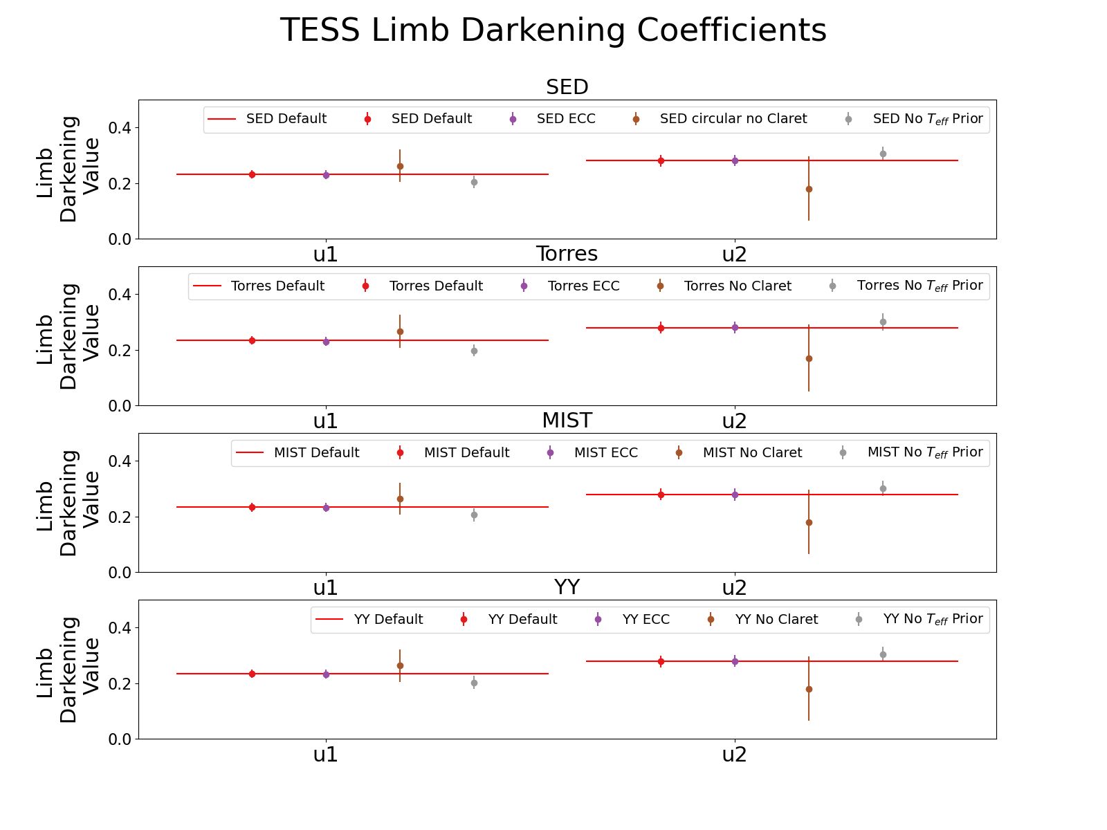
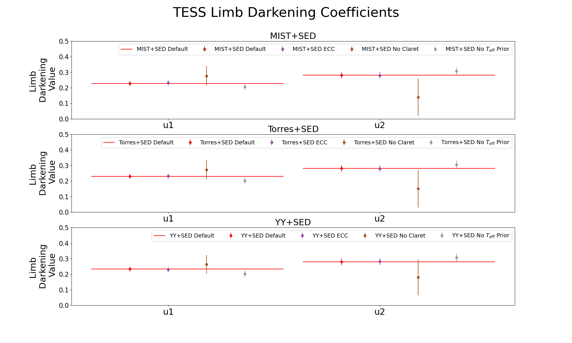
Figure 10: Limb darkening Fitting

5.3.2 The Results of Free Eccentricity

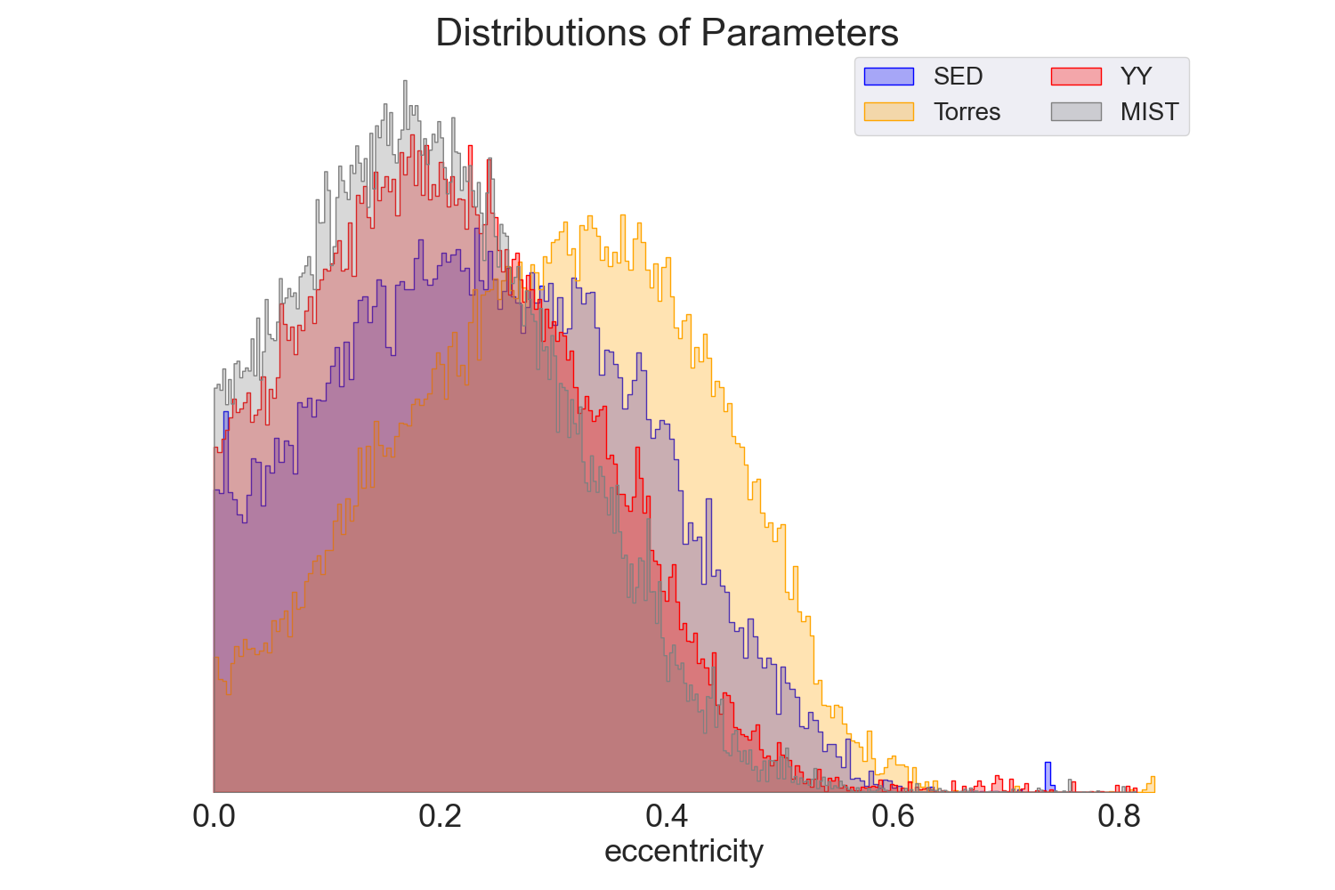
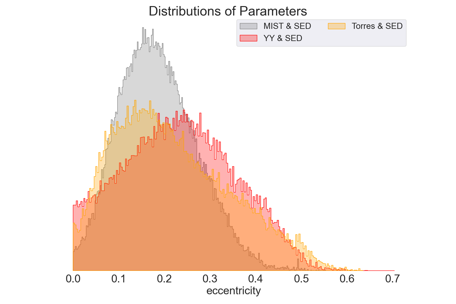
Figure 11: Comparison of eccentricity runs

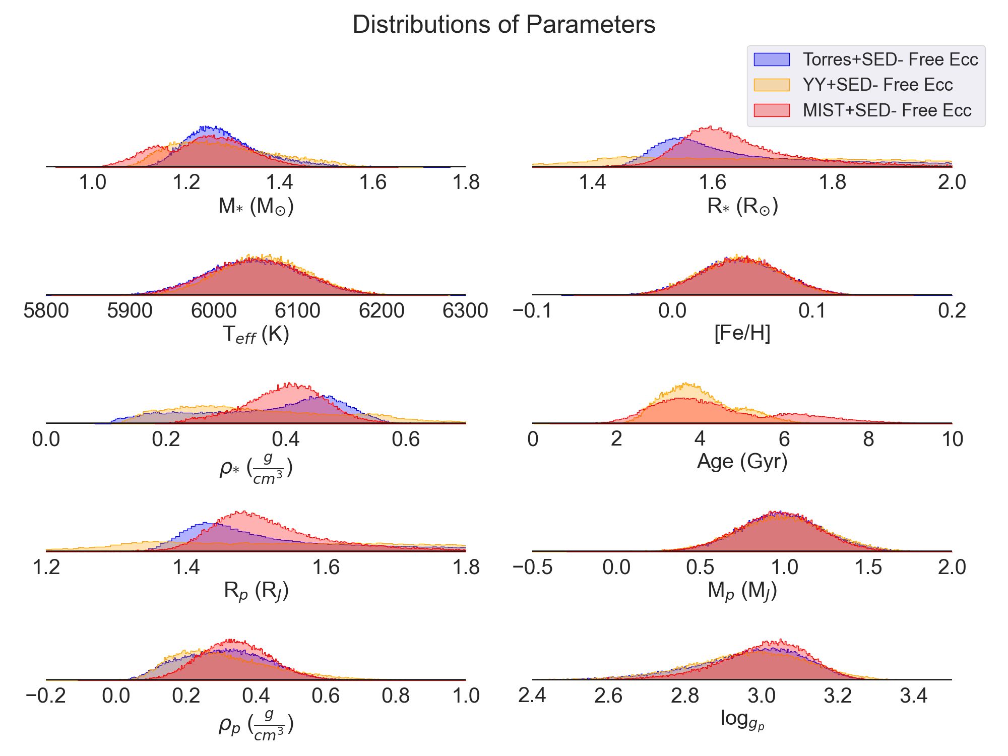
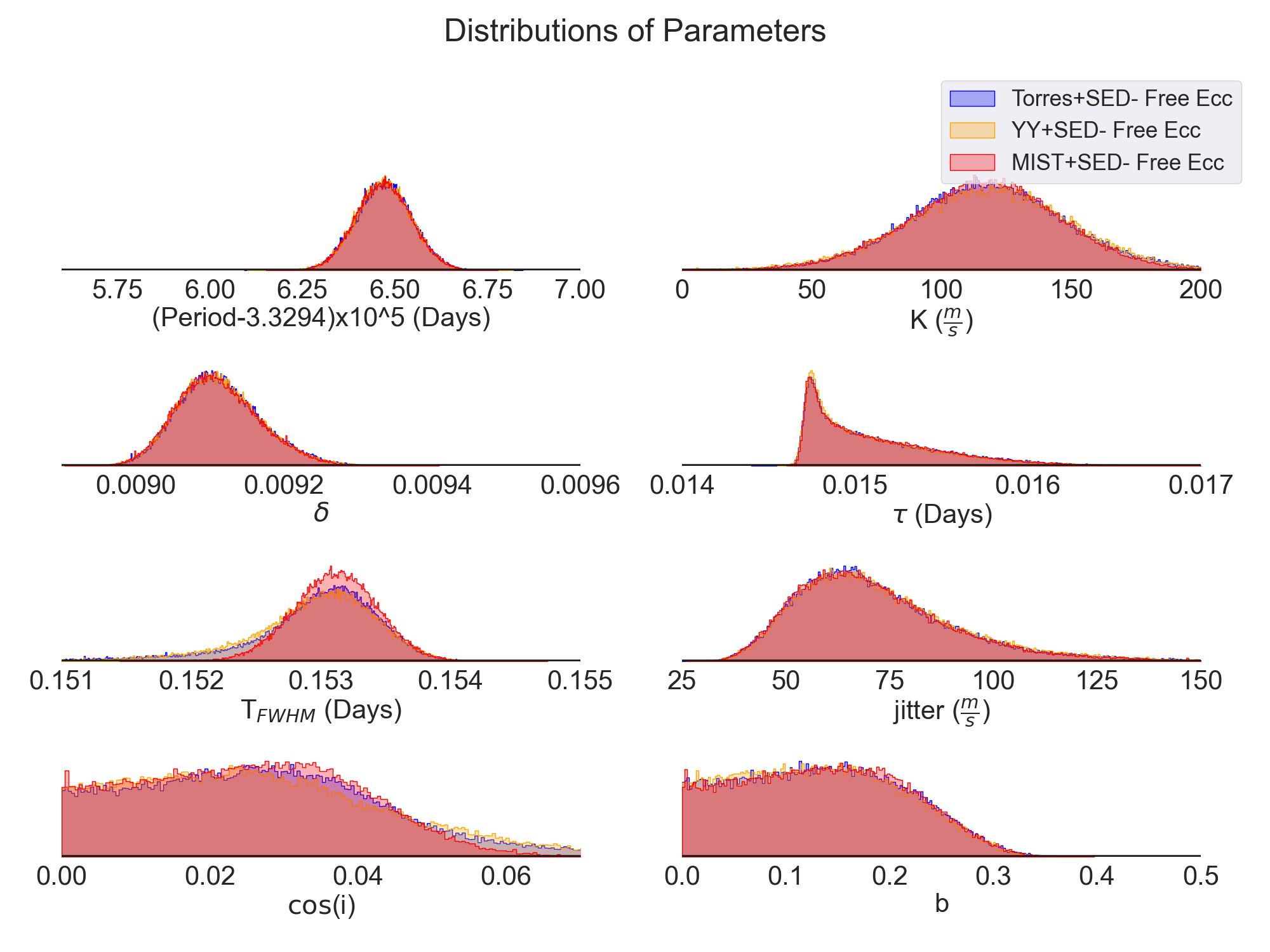
Figure 12: Posterior distribution of planet parameters when eccentricity is fit freely

In Figure 11 we show the posterior distributions for the eccentricities in the cases where they were freely fit. The abrupt cut off at zero in the shapes of our otherwise roughly Gaussian posterior distributions are a manifestation of the Lucy & Sweeney bias (Lucy & Sweeney, 1971), which pertains to a bias in inferred value of fitted parameters that are positive definite. In particular, the inferred eccentricities can have a value significantly different from zero, even if the intrinsic eccentricity is identically zero. All models except MIST + SED produce a median value that is consistent with zero to within $2.3\sigma$ of the uncertainty, which is the threshold for a significant non-zero eccentricity (Lucy & Sweeney, 1971). The MIST + SED with free eccentricity case has an eccentricity consistent with zero within 2.5 times its uncertainty. This is in line with Rodriguez et al. (2016) which also determined KELT-15b to have an orbit consistent with zero to within $2.3\sigma$.

However, many of our variations show that despite the eccentricity posterior distribution being consistent with zero, freely varying eccentricity has significant impacts on other system parameters. This results in a much less certain estimate of $R_{*}$ for YY and SED, which has an uncertainty 10 times greater than the circular YY and SED model, due to the increased uncertainty in $\rho_{*}$ when eccentricity is considered. We see a difference of 8.2% or $1.2\sigma$ in $R_{*}$ between the default MIST+SED model and the eccentric MIST+SED model. Predictably, we still see good agreement in the observable parameters as the estimates for effective temperature are largely unaffected by free eccentricity, leading to consistent limb darkening coefficients.

6 Discussion

In many ways KELT-15b (Rodriguez et al., 2016) is a hot Jupiter very typical of the population currently known. KELT-15b has a bright host star and a planetary radius comparable to Jupiter. There are many photometric transit observations, particularly from TESS. However, the radial velocity observations are limited to those presented in the discovery paper, used to confirm the planetary nature of the companion and provide only a rough estimate of the planet mass. The characteristics of this planet and its suite of observations make it a good proxy for most known hot Jupiters. Observations from TESS will continue to bolster this population by finding even more large planets around bright stars. In general, these planets will also have relatively few ground-based follow up radial velocity observations. The re-analysis of KELT-15b provides an excellent test-bed with which to explore the systematic biases present in the modeling of this population of transiting planets.

We find that the systematic offset in the host star and planetary parameters inferred using different methods of breaking the mass-radius degeneracy in transiting planet systems can be significant. For example we find differences as large as 5.9% or twice the largest uncertainty between the inferred stellar radii using different methods. This translates directly into a similar $2\sigma$ difference in the planetary radius. Given that we are entering an era of precision exoplanetology, where precise and accurate physical parameters of transiting planets are needed for planning and interpreting follow-up observations, this is a significant source of systematic error that must be accounted for. Based on this result, we argue that future efforts to precisely characterize the properties of transiting exoplanet systems must clearly explain the methodology by which they break the host star mass-radius degeneracy, as well as specify any explicit or implicit priors in their fits. In an era where the analysis of planetary interiors requires accurate radii and densities accurate to a few %, a $\sim 6\%$ difference caused by a largely unacknowledged source of systematic error is of concern.

Although we investigate the impacts of several different methods of breaking the mass-radius degeneracy in the host star and variations in a select set of our modelling assumptions, our study does not explore all possible sources of systematic error. For example, even within a given method of breaking the mass-radius degeneracy in the primary star, there can be significant variations in the inferred parameters. For example, Vines & Jenkins (2022) uses Bayesian Model Averaging in the python package ARIADNE to improve the SED fitting technique through incorporating information from 6 different stellar atmosphere models. Within these stellar atmospheres used for SED fitting, the authors find individual stellar atmosphere models can vary from interferometric radii by as much as 32%. They find their model averaging technique has a fractional difference of 0.001 $\pm$ 0.070 and has a mean precision of 2.1%. This shows that there can be significant improvements made to current methods of SED fitting techniques, which is just one method of breaking the mass-radius degeneracy.

The photometry included in the SED fits has also dramatically increased in volume in recent years. Yu et al. (2022) combined the data-sets from APOGEE (Abdurro’uf et al., 2022), GALAH (Buder et al., 2021), and RAVE (Steinmetz et al., 2020) to revise the radii for 1.5 million stars using the SED method on these photometric data-sets. They were able to use 32 photometric bands and the MARCS (Gustafsson et al., 2008) and BOSZ (Bohlin et al., 2017) model stellar atmospheres to fit the SEDs. With this detailed set of photometry for a large sample of targets, the researchers obtained radii that were consistent to 3% with CHARA (ten Brummelaar et al., 2005) interferometric radii. Overall their catalogue has a median precision of 3.6% in stellar radius. New observations from Gaia DR3 (Gaia Collaboration et al., 2022) will further enhance the widely available SED photometry by providing spectroscopic atmospheric parameters for 5.5 million stars.

Further studies have investigated the systematic uncertainties introduced by other methods of breaking the stellar mass-radius degeneracy. Our results of a difference of 5.9% or $2\sigma$ in $\rm R_{*}$ between several degeneracy breaking methods are in line with the results of Tayar et al. (2022). These authors find a floor of approximately 4% in stellar radius for solar type stars by comparing 4 different stellar evolution codes. This work examines the Yale Rotating Evolution Code Models (YREC) (Tayar & Pinsonneault, 2018), the MIST isochrones (Dotter, 2016), the Dartmouth Stellar Evolution Program (DSEP) (Dotter et al., 2008), and the Garching Stellar Evolution Code (GARSTEC) (Weiss & Schlattl, 2008; Serenelli et al., 2013). The only overlapping model with our analysis in the use of the MIST isochrones (Dotter, 2016), showing that we find similar results for a different suite of stellar modeling methods. This work focuses solely on the host stars and does not deeply investigate the impact on the transiting planets.

While the results of Tayar et al. (2022) and Vines & Jenkins (2022) explore the inference of different stellar properties for various stellar characterisation methods, we are able to see the full impact of these differences through modeling an entire system several times with different constraints. By globally modeling the system, we are capable of incorporating additional constraints on $\rho_{*}$ provided by the transit observations themselves. In the case of YY + SED we see that this model produced significant changes in the resulting posterior distributions compared to the other combination models, such as in a 3% fractional difference or $1\sigma$ in planetary radius compared to the MIST + SED estimate.

This analysis and similar results in the literature suggest the need for being very clear regarding the stellar characterisation method used to derive transiting exoplanet parameters. These systematic differences between the parameters inferred by different methods of breaking the mass-radius degeneracy and different priors make it difficult to compare populations of exoplanets that have been modelled using inhomogeneous methods. At minimum, it is important to include this systematic error caused by the differences between models into the error budget of the parameters of transiting planets, when attempting to draw comparisons between systems. Of course, this is complicated by the fact that these systematic errors are typically unquantified, something which we have aimed to rectify here.

6.1 The Effects of Claret Limb Darkening Models

When turning off the Claret Tables we see the largest differences in our “direct observables”. The direct observables are the parameters that are directly measured from observations and should not be effected by the selection of mass-radius degeneracy breaking method. These include: Period, transit depth $\delta$, $T_{fwhm}$, $\tau$, eccentricity, inclination, RV semi-amplitude $K$, $a/R_{*}$, $\log{g_{P}}$ and parallax. Since these direct observables are sensitive to the precise shape of the transit, they are sensitive to changes to the estimate of the limb darkening parameter, which characterizes the transit shape.

When we engage the Claret Tables in our “default” models, these direct observables are influenced by the estimated limb darkening parameters determined by the Claret tables as well as being constrained by the light curve itself. EXOFASTv2 applies a prior on the limb darkening coefficients based on the Claret Table value which depends on the stellar $T_{\rm eff}$ and $log{g_{*}}$. These limb darkening coefficients influence the estimates for the direct observables as seen in figure 9. The differences in the estimates of the fit limb darkening coefficients themselves for each variation are shown in figure 10. The work of Patel & Espinoza (2022) shows that even within methods of fitting limb darkening coefficients in transiting systems can lead to differing results. They find that using model atmospheres like PHOENIX can lead to discrepancies as large as ${\Delta_{u}}_{2}\sim 0.2$ when compared to empirical methods of determining limb darkening coefficients. This implies that changing the method of constraining the limb darkening coefficients could lead to even larger differences in the directly observable parameters than we observe.

However, the Claret Tables are not the only constraint on the limb darkening coefficients. Even in the absence of the Claret Tables, where the limb darkening parameters are fit more freely, we observe an influence from the estimate of the stellar density, $\rho_{*}$. In the case of our “default” single constraint models, excepting the SED, we do not have much additional information constraining the $T_{\rm eff}$ of the host star or the $\rho_{*}$ outside of the light curve itself. However, in the case of the combination models which use the indirect mass-radius degeneracy breaking methods and the SED, there are slightly more constraints on the limb darkening coefficients. Here, the SED provides additional information on $T_{\rm eff}$ and thus a weak constraint on $R_{*}$. This information combined with an estimate of [Fe/H] can be used to produce an estimate of $\rho_{*}$, that is roughly independent from the light curve. However, as shown in equation 4, $\rho_{*}$ can also be estimated solely from the direct observables given by the light curve (and RV data when the eccentricity is not fixed to 0). The tension from these two different estimates of $\rho_{*}$ exerts an influence on the fit of the limb darkening coefficients. This is to produce better agreement in the direct observables that constitute the second estimate of $\rho_{*}$ with the $T_{\rm eff}$ dependent estimate of $\rho_{*}$. Larger or smaller estimates of a limb darkening coefficient would imply changes to the shape of the light curve. This would lead to changes in the estimates of the direct observable that depend on the shape of the light curve. We see this effect is especially prominent when we remove the constraints of the Claret Tables. Thus the differences in the fit limb darkening coefficients, produced by engaging the Claret tables or not, influence the fit of the direct observables as shown in figure 9. We see this effect can produce changes as large as $1.4\sigma$ in $T_{\rm FWHM}$.

6.2 Effects of Free Eccentricity

We observe more consistent agreement in the directly observable parameters when using the eccentric combination constraint models, shown in figure 12, than when employing the “default” combination constrains, shown in figure 5, which assumes circular orbits. Equation 1 shows the clear dependence between the semi amplitude K and eccentricity. Through equation 3 we see relationships between many of our directly observed quantities and eccentricity. Thus by adding eccentricity as a free parameter, we would expect to observe changes in these directly observed quantities. As explored in section 6.1, the discussion of the effects of employing the Claret tables to fit limb darkening coefficients, we see that combining our indirect degeneracy breaking methods with the SED provides a stronger constraint on the $T_{\rm eff}$ and a weak constraint on $R_{*}$. Then, since the Claret tables are engaged there is a tension between the stellar radius estimated by the $T_{\rm eff}$ and the stellar radius estimated by calculating $\rho_{*}$ from the observables. Here the eccentricity, as a free parameter, can ameliorate the tension between these estimates. This results in consistent values for the directly observable parameters across models by estimating the value of the eccentricity. With slight changes in the estimated value, the eccentricity can absorb the tension in $\rm rho_{*}$. As a result, the directly observed parameters settle around more consistent values without the tensions in the competing estimates of $\rm\rho_{*}$. We see a reduction in spread of the transit depth from 0.3% or $0.4\sigma$ in the “default” combination models compared to no spread in the free eccentricity combination models.

In addition, hot Jupiters are often assumed to have circular orbits. However, we see in our variation analysis that modeling for eccentricity, even when that eccentricity is consistent with zero within 2.3$\sigma$, provides a host of changes in system parameters and increases the uncertainties of parameters that may still be consistent with the circular fit. For example, the uncertainty in $R_{*}$ goes from 2.9% in the “default” MIST+SED combination model to 6.2% in the eccentric MIST+SED model. There is an equivalent increase in uncertainty in $R_{p}$. Where we see a 3.1% uncertainty in the circular case and an 6.1% uncertainty in the eccentric case. Imposing the constraint of a circular orbit is observed to be a strong prior, which should encourage caution in its use. When attempting to draw an accurate picture of the error budgets of an exoplanet system, it is important to consider that the tight constraint on a circular orbit may be artificially constricting the uncertainty ranges for these other inferred parameters.

6.3 Effects of Combination Constraints on Direct Observables

Even in maintaining our “default” assumptions of engaging the Claret tables and assuming circular orbits, we still see shifts in the direct observables in our combination constraint models depending on the mass-radius degeneracy breaking method. In these models we use both an indirect constraint (MIST, YY, the Torres relations) and the SED of the host star. We still engage the Claret tables and assume a circular orbit. In our single constraint “default” models we see nearly perfect agreement in the direct observables, regardless of the degeneracy breaking method used. However, in the combination models we do see minor differences in some of the directly observable parameters.

For example, the YY and SED combination constraint models produce a value of the transit depth $\delta$ that is shallower than the MIST and SED by $0.4\sigma$. In these combination methods, this difference is due a tension in the estimate of the stellar density. The SED supplies increased information in the $T_{\rm eff}$ of the host star and an $R_{*}$ estimate when combined with a parallax. The degeneracy breaking methods each describe a relationship between $\rm R_{*}$ and $\rm M_{*}$. When this relationship is combined with the SED estimate of $\rm R_{*}$, $\rho_{*}$ can be estimated independently of the light curve. However, we can still constrain $\rho_{*}$ purely from the light curve as shown in equation 4. If these estimates are not in perfect agreement, the competing approaches to $\rho_{*}$ can introduce a tension in fitting the direct observables used to estimate $\rho_{*}$. Additionally, when using the Claret Tables, EXOFASTv2 applies a prior on the limb darkening coefficients based on the value given by the Claret Tables for the specified $T_{\rm eff}$, [Fe/H], and $\log{g}$. Thus the Claret Tables influence the fit of the limb darkening coefficients and the direct observables which contribute to $\rho_{*}$.

Accordingly, The YY and SED combination constraint model produces a temperature that is significantly lower than the MIST and SED by $0.8\sigma$. This is followed by a $0.6\sigma$ difference in $\rho_{*}$, which depends on the direct observables, and is now influenced by the temperature estimate from our mass-radius degeneracy breaking models. We see a similar tension to that observed in the models not employing the Claret tables at all. Here, we do see a change in the limb darkening coefficients in the TESS band-pass given by the Claret tables between the MIST and SED and the YY and SED of $0.3\sigma$ for the first term and $0.1\sigma$ for the second term. The change in limb darkening depending on the temperature estimates from the indirect method and the SED would be responsible for the changes in the direct observables. Our single constraint models, excepting SED, do not provide additional temperature information. There we see effectively no spread based on degeneracy breaking model in our direct observables with changes of $0.06\sigma$ and $0.05\sigma$ respectively for the two limb darkening coefficients between MIST and SED.

6.4 Best Practices and Future Work

Based on the results of our analysis, we offer several suggestions for “best practices” when analyzing transiting planet systems. We find that the inclusion or exclusion of limb darkening models has important impacts on direct observables like the measured transit depth and duration. We find that providing a spectroscopic prior on $T_{\rm eff}$ generally improves the precision on the estimates of $M_{*}$, $R_{*}$ and $R_{p}$, particularly for the single constraint Torres, MIST, and YY models, for which there does not exist a unique solution to the system without a $T_{\rm eff}$ prior, ignoring the weak constraint on $T_{\rm eff}$ from limb darkening. We find that, even when including the SED, whose shape provides an independent constraint on $T_{\rm eff}$, applying the spectroscopic constraint on $T_{\rm eff}$ results in smaller statistical uncertainties on $M_{*}$, $R_{*}$, and $R_{p}$. However, systematics in the spectroscopically-measured $T_{\rm eff}$ should be considered (Tayar et al., 2022) and may imply that the prior on the spectroscopically-derived $T_{\rm eff}$ should not be included (Eastman et al., in prep).

When SED information is available, we recommend combining it with another method of breaking the host star mass and radius degeneracy. SED alone produces one of the least precise estimates for the mass and radius of the host star. When combined with another method, its precision increases by a fractional difference of 30% in the stellar radius when combined in conjunction with the YY, while still retaining the benefits of an empirical measurement. Although we do not see the same level uncertainty improvement when the MIST isochrones and the SED are combined, the median value clusters more closely to the other models than did the estimates produced by MIST or SED alone. We also encourage the consideration of both circular and eccentric orbits as we show the effects these different eccentricity assumptions can have on a variety of different planet parameters. Even when eccentricities are consistent with zero, we see significant increases in uncertainty for several derived parameters like $R_{*}$ and $R_{p}$. By applying the constraint of a circular orbit as a matter of course, the uncertainties in these derived parameters could be artificially constrained. This is an important consideration when attempting an accurate accounting of the error budget of a planetary system.

Above all, we strongly encourage exoplanet researchers to report in detail which method of host star characterisation is being used in deriving physical planet parameters, as well as their prior assumptions. Currently there is no central database of the method used for host star characterisation, making it difficult to understand the prevalence of these different methods of breaking the mass-radius degeneracy. The opacity of these methods increases the difficulty of comparing wide selections of planets and applying additional systematic uncertainties caused by these inhomogeneous methods.

This work also highlights the importance of globally modeling both the host star and transiting planet simultaneously. We have found several instances where changes in the information being applied to the host star such as providing a prior on $T_{\rm eff}$, the method used to fit limb darkening coefficients, or combining indirect stellar characterisation methods with the SED, produce significant differences in the directly observable and the inferred properties of the transiting planet. Many of these effects would not have been considered if we had sequentially and independently modelled the host star then the transiting planet. For example, fitting the host star independently from the planet completely elides the role the host star’s properties play in fitting the “directly” observable parameters. We would not consider the ability of the light curve direct observables to assist in constraining $\rho_{*}$ rather than solely relying on the derived estimate from the effective temperature. This important independent constraint would then be lost. As discussed in section 6.1, the tension between the $\rho_{*}$ estimated by $T_{\rm eff}$ and the $\rho_{*}$ estimated by the light curve, are significant factors in fitting the direct observables. These observables in turn are then used to estimated the derived quantities like $R_{*}$ and $R_{p}$. Thus we incorporate far more information to accurately characterise the host star and transiting planet when we model these systems simultaneously and globally.

In the future, we hope to apply this analysis to a set of benchmark systems, i.e., bright host stars with observations from Gaia (Gaia Collaboration et al., 2016b) or SPHEREX (Doré et al., 2018), host stars with interferometrically measured radii, stars with asteroseismologically-inferred masses and radii, and those with ”flicker”-based estimates of $\log{g_{*}}$. This would allow us to compare these models to not only each other but to an approximation of the ground truth for stellar radii.

7 Conclusions

With increased ability to carefully characterize the atmospheres and interior compositions of exoplanets, precise and accurate measurements of the physical parameters of exoplanets are invaluable. When characterizing planets using transit and radial velocity observations there exists a fundamental degeneracy between the mass and the radius of the host star (Seager & Mallén-Ornelas, 2003). Breaking this degeneracy is needed to translate proportional observations of planets into physical units. However, to date, several inhomogenous methods have been employed to break this degeneracy in stellar properties. We have used KELT-15b (Rodriguez et al., 2016) as a test bed to compare the results for exoplanet characterisation using 4 single constraint models: the SED in combination with Gaia parallax, the MIST isochrones (Dotter, 2016), the YY isochrones (Yi et al., 2001), and the semi-empirical Torres relations (Torres et al., 2009). We also investigate the combination of the indirect models (MIST, YY, the Torres relations) with the SED, and finally three variations on each of these 7 models, testing underlying the assumptions on eccentricity, the $T_{\rm eff}$ prior, and the method of fitting the limb darkening coefficients. We list several important conclusions:

• The inclusion of TESS data improves our precision on planet period by 50% - Section 5

• Simultaneously fitting the host star and planet allow for stellar properties like $\rm\rho_{*}$ to be constrained by both direct observable parameters and independent estimates from $T_{\rm eff}$ and the mass-radius degeneracy breaking method used - Section 6.1

• The method used to step through a parameter such as stepping linearly in $K$ or in $\log(K)$, can have small but significant variations in the best fit parameters - Section 3

• Our single constraint models display a 5.9% or a $2\sigma$ change in planetary radius between the smaller MIST estimate and larger SED estimate - Section 5.1

• We find significant changes in the “directly” observed parameters in our combination constraint models as well as a 3% or $1\sigma$ spread in the planetary radius - Section 5.2

• We find that the decision to employ the Claret limb darkening tables (Claret, 2017) or not provides a modest but noticeable effect on the ”directly” observable parameters - Section 6.1

• Even in systems with eccentricities consistent with zero within 2.3-$\sigma$, imposing circular orbit constraints routinely may artificially constrain the uncertainty in many parameters - Section 6.2

• We encourage exoplanet researchers to consistently report the mass-radius degeneracy breaking method used to characterise their host stars and for this information to be stored in a database - Section 6.4

By comparing the derived planetary properties when applying these different mass-radius degeneracy breaking methods to the host star, we see several stark differences. We find that the MIST isochrones produce the smallest stellar mass and radius which translates directly to the smallest planetary radius. Conversely, the SED and Gaia parallax method produces the largest estimates of these parameters. We see a fractional difference of 5.9% or $2\sigma$, twice larger of the statistical uncertainties, in planetary radius between these two methods of breaking the degeneracy between the mass and the radius of the host star. This is an important source of systematic error, at the level of twice our statistical error, which should be considered when comparing exoplanets whose physical properties have been derived using inhomogeneous methods.

We also combine several of these methods and compare the impacts on the derived planetary properties. These models include the MIST+SED, YY+SED, and Torres+SED. We see the largest estimates for stellar mass and radius in this set from the MIST and SED combination and the smallest from the YY and SED, with the semi-empirical Torres relations and the SED falling between these two. This results in a spread of 3% or $1\sigma$, at the same level as the statistical uncertainty, in $R_{*}$ and 5.6% or $0.86\sigma$ in $M_{*}$. These combination results do remain in the region between the MIST single-constraint result and the SED single-constraint result.

Finally we explore three variations of all seven models by exploring freely varying the eccentricity, not applying the Claret limb darkening tables, or only applying a starting value for the $T_{\rm eff}$ instead of a prior complete with an uncertainty. Generally, we find most of the models are very sensitive to whether or not a prior on $T_{\rm eff}$ is adopted. The MIST and SED combination is the most robust against this change. We find that the use of the Claret tables to fit limb darkening coefficients compared to fitting these parameters freely has the largest impact on the determination of the transit duration, and other directly observed parameters due to tensions in fitting $\rho_{*}$. We find the most significant change in many parameters by allowing the eccentricity to vary freely. The eccentricity fit for all seven models is consistent with zero within $2.5\sigma$. The stellar density as described in equations 3 and 4, show the dependency of the stellar density on a well characterised eccentricity. Nevertheless, freely varying the eccentricity introduces significant uncertainty in the stellar radius in almost all of our models. By not routinely fitting for eccentricity in hot Jupiters, we may be artificially constraining the uncertainties of their derived properties, even in systems with eccentricities consistent with zero.

In the future, a consistently agreed-upon method for breaking the mass-radius degeneracy is essential to the comparative study of exoplanets. This would reduce the role of systematic errors when making detailed comparisons between exoplanets. If a consistent model is not used, detailing which host star mass-radius degeneracy breaking method is used is necessary to be able to account for the systematic differences outlined in this work. Future studies would be recommended to apply these methods to a wider sample benchmark systems with constraints from, e.g., interferometery, asteroseismology, or other direct empirically constraints. This would provide a pathway to defining a method of analyzing transiting planets that is most consistent with ground truth.

Acknowledgements

Some/all of the data presented in this paper were obtained from the Mikulski Archive for Space Telescopes (MAST). Other data is available upon request.

Table 5: Results for circular single constraint models

	MIST	YY	Torres	SED	Range	Units
$M_{*}$	$1.165^{+0.086}_{-0.093}$	$1.187^{+0.041}_{-0.056}$	$1.213^{+0.057}_{-0.053}$	$1.38^{+0.12}_{-0.11}$	$0.215$	$(\,M_{\sun})$
$R_{*}$	$1.44^{+0.041}_{-0.042}$	$1.447^{+0.028}_{-0.025}$	$1.46^{+0.031}_{-0.027}$	$1.525^{+0.04}_{-0.036}$	$0.085$	$(\,R_{\sun})$
$L_{*}$	$2.48^{+0.2}_{-0.19}$	$2.49^{+0.17}_{-0.15}$	$2.56^{+0.17}_{-0.15}$	$2.82^{+0.16}_{-0.12}$	$0.34$	$(\,L_{\sun})$
$\rho_{*}$	$0.553^{+0.013}_{-0.025}$	$0.553^{+0.014}_{-0.025}$	$0.553^{+0.014}_{-0.025}$	$0.553^{+0.014}_{-0.025}$	$0$	$g~{}cm^{-3}$
$\log{g}$	$4.187^{+0.013}_{-0.015}$	$4.1903^{+0.0092}_{-0.013}$	$4.1938^{+0.0099}_{-0.013}$	$4.214^{+0.016}_{-0.021}$	$0.027$	(cgs)
$T_{\rm eff}$	$6039.0^{+59.0}_{-59.0}$	$6028.0^{+60.0}_{-55.0}$	$6043.0^{+60.0}_{-59.0}$	$6059.0^{+56.0}_{-55.0}$	$31$	(K)
$[{\rm Fe/H}]$	$0.049^{+0.03}_{-0.03}$	$0.045^{+0.03}_{-0.03}$	$0.048^{+0.03}_{-0.03}$	$0.049^{+0.03}_{-0.03}$	$0.004$	(dex)
$Age$	$4.8^{+2.5}_{-1.6}$	$4.37^{+1.2}_{-0.6}$	N/A	N/A	$0.43$	Age (Gyr)
$P$	$3.32946469^{+7.6e-07}_{-7.6e-07}$	$3.32946468^{+7.5e-07}_{-7.5e-07}$	$3.32946468^{+7.6e-07}_{-7.5e-07}$	$3.32946468^{+7.6e-07}_{-7.6e-07}$	$0$	Period (days)
$R_{P}$	$1.337^{+0.04}_{-0.039}$	$1.343^{+0.03}_{-0.024}$	$1.355^{+0.032}_{-0.026}$	$1.417^{+0.037}_{-0.034}$	$0.08$	$(\,R_{\rm J})$
$M_{P}$	$0.84^{+0.22}_{-0.24}$	$0.85^{+0.22}_{-0.23}$	$0.87^{+0.22}_{-0.24}$	$0.95^{+0.25}_{-0.26}$	$0.11$	$(\,M_{\rm J})$
$T_{C}$	$2458534.08842^{+0.00014}_{-0.00014}$	$2458534.08842^{+0.00013}_{-0.00014}$	$2458534.08842^{+0.00013}_{-0.00014}$	$2458534.08841^{+0.00013}_{-0.00014}$	$1e-05$	Time of conjunction ($\rm{BJD_{TDB}}$)
$T_{T}$	$2458534.08842^{+0.00014}_{-0.00014}$	$2458534.08842^{+0.00013}_{-0.00014}$	$2458534.08842^{+0.00013}_{-0.00014}$	$2458534.08841^{+0.00013}_{-0.00014}$	$1e-05$	Time of minimum projected separation ($\rm{BJD_{TDB}}$)
$T_{0}$	$2458926.96525^{+0.0001}_{-0.0001}$	$2458930.29472^{+0.0001}_{-0.0001}$	$2458926.96525^{+0.0001}_{-0.0001}$	$2458923.63577^{+0.0001}_{-0.0001}$	$6.65895$	Optimal conjunction Time ($\rm{BJD_{TDB}}$)
$a$	$0.0459^{+0.0011}_{-0.0013}$	$0.04621^{+0.00052}_{-0.00074}$	$0.04655^{+0.00072}_{-0.00069}$	$0.0486^{+0.0014}_{-0.0013}$	$0.003$	Semi-major axis (AU)
$i$	$88.84^{+0.76}_{-0.74}$	$88.83^{+0.77}_{-0.75}$	$88.82^{+0.76}_{-0.74}$	$88.83^{+0.77}_{-0.74}$	$0.02$	Inclination (Degrees)
$T_{eq}$	$1631.0^{+19.0}_{-18.0}$	$1628.0^{+20.0}_{-17.0}$	$1632.0^{+19.0}_{-18.0}$	$1636.0^{+19.0}_{-17.0}$	$8$	(K)
$\tau_{\rm circ}$	$0.122^{+0.033}_{-0.035}$	$0.121^{+0.033}_{-0.034}$	$0.12^{+0.032}_{-0.034}$	$0.115^{+0.03}_{-0.032}$	$0.007$	Tidal circularization timescale (Gyr)
$K$	$103.0^{+26.0}_{-29.0}$	$103.0^{+26.0}_{-29.0}$	$104.0^{+26.0}_{-29.0}$	$103.0^{+26.0}_{-28.0}$	$1$	(m/s)
$R_{P}/R_{*}$	$0.09542^{+0.00033}_{-0.00028}$	$0.09542^{+0.00033}_{-0.00028}$	$0.09542^{+0.00033}_{-0.00028}$	$0.09542^{+0.00033}_{-0.00028}$	$0$	Radius of planet in stellar radii
$a/R_{*}$	$6.872^{+0.055}_{-0.1}$	$6.871^{+0.056}_{-0.1}$	$6.87^{+0.056}_{-0.1}$	$6.871^{+0.056}_{-0.1}$	$0.002$	Semi-major axis in stellar radii
$\delta$	$0.009105^{+6.3e-05}_{-5.3e-05}$	$0.009105^{+6.3e-05}_{-5.3e-05}$	$0.009104^{+6.4e-05}_{-5.3e-05}$	$0.009105^{+6.4e-05}_{-5.3e-05}$	$0$	Transit depth (fraction)
$Depth$	$0.009105^{+6.3e-05}_{-5.3e-05}$	$0.009105^{+6.3e-05}_{-5.3e-05}$	$0.009104^{+6.4e-05}_{-5.3e-05}$	$0.009105^{+6.4e-05}_{-5.3e-05}$	$0$	Flux decrement at mid transit
$\tau$	$0.01502^{+0.00054}_{-0.00027}$	$0.01502^{+0.00054}_{-0.00028}$	$0.01502^{+0.00054}_{-0.00028}$	$0.01502^{+0.00054}_{-0.00028}$	$0$	ingress/egress transit duration (days)
$T_{14}$	$0.16834^{+0.00047}_{-0.00039}$	$0.16834^{+0.00048}_{-0.0004}$	$0.16835^{+0.00047}_{-0.00039}$	$0.16834^{+0.00047}_{-0.00039}$	$0$	Total transit duration (days)
$T_{FWHM}$	$0.15325^{+0.00031}_{-0.00031}$	$0.15324^{+0.00031}_{-0.00031}$	$0.15325^{+0.00031}_{-0.00031}$	$0.15324^{+0.00031}_{-0.00031}$	$0$	FWHM transit duration (days)
$b$	$0.14^{+0.086}_{-0.091}$	$0.14^{+0.086}_{-0.091}$	$0.141^{+0.085}_{-0.09}$	$0.141^{+0.086}_{-0.091}$	$0.001$	Transit Impact parameter
$\delta_{S,2.5\mu m}$	$437.0^{+16.0}_{-13.0}$	$436.0^{+16.0}_{-12.0}$	$438.0^{+17.0}_{-13.0}$	$440.0^{+16.0}_{-12.0}$	$4$	Blackbody eclipse depth at 2.5$\mu$m (ppm)
$\delta_{S,5.0\mu m}$	$1145.0^{+27.0}_{-18.0}$	$1143.0^{+27.0}_{-18.0}$	$1146.0^{+27.0}_{-18.0}$	$1148.0^{+27.0}_{-17.0}$	$5$	Blackbody eclipse depth at 5.0$\mu$m (ppm)
$\delta_{S,7.5\mu m}$	$1512.0^{+30.0}_{-18.0}$	$1511.0^{+30.0}_{-18.0}$	$1513.0^{+30.0}_{-19.0}$	$1515.0^{+30.0}_{-18.0}$	$4$	Blackbody eclipse depth at 7.5$\mu$m (ppm)

Table 6: Continuation of results for the circular single constraint models

	MIST	YY	Torres	SED	Range	Units
$\rho_{P}$	$0.44^{+0.11}_{-0.12}$	$0.43^{+0.11}_{-0.12}$	$0.43^{+0.11}_{-0.12}$	$0.41^{+0.11}_{-0.11}$	$0.03$	Density ($g~{}cm^{-3}$)
$logg_{P}$	$3.068^{+0.099}_{-0.14}$	$3.068^{+0.099}_{-0.14}$	$3.069^{+0.096}_{-0.14}$	$3.068^{+0.098}_{-0.14}$	$0.001$	Surface gravity
$\Theta$	$0.05^{+0.013}_{-0.014}$	$0.049^{+0.013}_{-0.014}$	$0.049^{+0.012}_{-0.014}$	$0.047^{+0.012}_{-0.013}$	$0.003$	Safronov Number
$\langle F\rangle$	$1.605^{+0.078}_{-0.07}$	$1.594^{+0.078}_{-0.067}$	$1.611^{+0.078}_{-0.072}$	$1.627^{+0.075}_{-0.067}$	$0.033$	Incident Flux (109 erg s-1 cm-2)
$T_{P}$	$2458534.08842^{+0.00014}_{-0.00014}$	$2458534.08842^{+0.00013}_{-0.00014}$	$2458534.08842^{+0.00013}_{-0.00014}$	$2458534.08841^{+0.00013}_{-0.00014}$	$1e-05$	Time of Periastron ($\rm{BJD_{TDB}}$)
$T_{S}$	$2458535.75315^{+0.00014}_{-0.00014}$	$2458532.42369^{+0.00014}_{-0.00014}$	$2458535.75315^{+0.00013}_{-0.00014}$	$2458535.75314^{+0.00013}_{-0.00014}$	$3.32946$	Time of eclipse ($\rm{BJD_{TDB}}$)
$T_{A}$	$2458536.58552^{+0.00014}_{-0.00014}$	$2458536.58552^{+0.00013}_{-0.00014}$	$2458536.58551^{+0.00013}_{-0.00014}$	$2458536.5855^{+0.00013}_{-0.00014}$	$2e-05$	Time of Ascending Node ($\rm{BJD_{TDB}}$)
$T_{D}$	$2458534.92079^{+0.00014}_{-0.00014}$	$2458534.92079^{+0.00013}_{-0.00014}$	$2458534.92078^{+0.00013}_{-0.00014}$	$2458534.92077^{+0.00013}_{-0.00014}$	$2e-05$	Time of Descending Node ($\rm{BJD_{TDB}}$)
$vcve_{0}$	$1.0^{+0.0}_{-0.0}$	$1.0^{+0.0}_{-0.0}$	$1.0^{+0.0}_{-0.0}$	$1.0^{+0.0}_{-0.0}$	$0$
$M_{P}\sin i$	$0.84^{+0.22}_{-0.24}$	$0.85^{+0.22}_{-0.23}$	$0.87^{+0.22}_{-0.24}$	$0.95^{+0.25}_{-0.26}$	$0.11$	Minimum mass ($\,M_{\rm J}$)
$d/R_{*}$	$6.872^{+0.055}_{-0.1}$	$6.871^{+0.056}_{-0.1}$	$6.87^{+0.056}_{-0.1}$	$6.871^{+0.056}_{-0.1}$	$0.002$	Separation at mid transit
$P_{T}$	$0.1316^{+0.002}_{-0.001}$	$0.1316^{+0.002}_{-0.001}$	$0.1317^{+0.002}_{-0.001}$	$0.1317^{+0.002}_{-0.001}$	$0$	A priori non-grazing transit prob
$P_{T,G}$	$0.1594^{+0.0025}_{-0.0013}$	$0.1594^{+0.0025}_{-0.0013}$	$0.1594^{+0.0025}_{-0.0013}$	$0.1594^{+0.0025}_{-0.0013}$	$0$	A priori transit prob
$u_{1}$	$0.244^{+0.045}_{-0.045}$	$0.245^{+0.045}_{-0.045}$	$0.244^{+0.045}_{-0.045}$	$0.242^{+0.045}_{-0.045}$	$0.003$	Band: V ICO
$u2_{0}$	$0.299^{+0.048}_{-0.048}$	$0.298^{+0.048}_{-0.048}$	$0.299^{+0.047}_{-0.048}$	$0.3^{+0.048}_{-0.048}$	$0.002$	Band: V ICO
$u1_{1}$	$0.32^{+0.049}_{-0.05}$	$0.32^{+0.049}_{-0.049}$	$0.319^{+0.048}_{-0.049}$	$0.316^{+0.049}_{-0.049}$	$0.004$	Band: R ICO
$u2_{1}$	$0.297^{+0.05}_{-0.049}$	$0.296^{+0.049}_{-0.05}$	$0.298^{+0.05}_{-0.05}$	$0.298^{+0.05}_{-0.05}$	$0.002$	Band: R ICO
$u1_{2}$	$0.233^{+0.016}_{-0.016}$	$0.234^{+0.016}_{-0.016}$	$0.234^{+0.015}_{-0.016}$	$0.232^{+0.015}_{-0.015}$	$0.002$	Band: I PEST
$u2_{2}$	$0.279^{+0.021}_{-0.021}$	$0.278^{+0.021}_{-0.021}$	$0.279^{+0.021}_{-0.021}$	$0.28^{+0.021}_{-0.021}$	$0.002$	Band: I PEST
$u1_{3}$	$0.43^{+0.047}_{-0.047}$	$0.43^{+0.047}_{-0.047}$	$0.43^{+0.046}_{-0.047}$	$0.427^{+0.047}_{-0.046}$	$0.003$	Band: TESS
$u2_{3}$	$0.301^{+0.049}_{-0.049}$	$0.301^{+0.049}_{-0.049}$	$0.303^{+0.049}_{-0.048}$	$0.303^{+0.048}_{-0.048}$	$0.002$	Band: TESS
$\gamma_{\rm rel_{0}}$	$12195.0^{+21.0}_{-21.0}$	$12196.0^{+20.0}_{-20.0}$	$12195.0^{+20.0}_{-20.0}$	$12195.0^{+20.0}_{-21.0}$	$1$	Relative RV Offset (m/s)
$\sigma_{J_{0}}$	$65.0^{+22.0}_{-15.0}$	$65.0^{+22.0}_{-15.0}$	$65.0^{+22.0}_{-15.0}$	$65.0^{+22.0}_{-15.0}$	$0$	RV Jitter (m/s)
${\sigma_{J}}^{2}_{0}$	$4300.0^{+3400.0}_{-1700.0}$	$4300.0^{+3400.0}_{-1700.0}$	$4300.0^{+3400.0}_{-1700.0}$	$4300.0^{+3300.0}_{-1700.0}$	$0$	RV Jitter Variance
${\gamma_{\rm rel}}_{1}$	$12194.0^{+23.0}_{-21.0}$	$12194.0^{+23.0}_{-21.0}$	$12194.0^{+23.0}_{-21.0}$	$12194.0^{+23.0}_{-21.0}$	$0$
${\sigma_{J}}_{1}$	$12.2^{+7.7}_{-12.0}$	$12.0^{+7.9}_{-12.0}$	$12.3^{+7.7}_{-12.0}$	$12.1^{+7.8}_{-12.0}$	$0.3$
${\sigma_{J}^{2}}_{1}$	$150.0^{+250.0}_{-340.0}$	$140.0^{+250.0}_{-340.0}$	$150.0^{+250.0}_{-340.0}$	$150.0^{+250.0}_{-340.0}$	$10$
$variance_{0}$	$1.47e-05^{+1.2e-06}_{-1.1e-06}$	$1.47e-05^{+1.2e-06}_{-1.1e-06}$	$1.47e-05^{+1.2e-06}_{-1.1e-06}$	$1.47e-05^{+1.2e-06}_{-1.1e-06}$	$0$
$f0_{0}$	$1.00389^{+0.00021}_{-0.00021}$	$1.00388^{+0.00021}_{-0.00021}$	$1.00389^{+0.00021}_{-0.00022}$	$1.00389^{+0.00021}_{-0.00021}$	$0$	Baseline flux
${C0_{0}}_{0}$	$-0.01074^{+0.00065}_{-0.00065}$	$-0.01074^{+0.00065}_{-0.00065}$	$-0.01074^{+0.00065}_{-0.00065}$	$-0.01074^{+0.00065}_{-0.00065}$	$0$	Additive detrending coeff
${C1_{0}}_{1}$	$0.00109^{+0.00034}_{-0.00034}$	$0.00109^{+0.00034}_{-0.00034}$	$0.00109^{+0.00034}_{-0.00034}$	$0.00109^{+0.00034}_{-0.00033}$	$0$	Additive detrending coeff

Table 7: Results for eccentric single constraint models

	MIST Eccentric	YY Eccentric	Torres Eccentric	SED Eccentric	Range	Units
$M_{*}$	$1.22^{+0.15}_{-0.12}$	$1.226^{+0.12}_{-0.082}$	$1.316^{+0.1}_{-0.091}$	$0.91^{+0.57}_{-0.38}$	$0.406$	$(\,M_{\sun})$
$R_{*}$	$1.56^{+0.34}_{-0.2}$	$1.61^{+0.33}_{-0.21}$	$1.91^{+0.37}_{-0.34}$	$1.527^{+0.039}_{-0.037}$	$0.383$	$(\,R_{\sun})$
$L_{*}$	$2.93^{+1.4}_{-0.71}$	$3.08^{+1.5}_{-0.79}$	$4.4^{+1.9}_{-1.4}$	$2.82^{+0.16}_{-0.13}$	$1.58$	$(\,L_{\sun})$
$\rho_{*}$	$0.45^{+0.18}_{-0.17}$	$0.41^{+0.19}_{-0.16}$	$0.267^{+0.18}_{-0.099}$	$0.36^{+0.22}_{-0.15}$	$0.183$	($g~{}cm^{-3}$)
$\log{g}$	$4.135^{+0.091}_{-0.13}$	$4.11^{+0.1}_{-0.13}$	$4.0^{+0.14}_{-0.13}$	$4.03^{+0.21}_{-0.24}$	$0.135$	(cgs)
$T_{\rm eff}$	$6039.0^{+60.0}_{-58.0}$	$6035.0^{+59.0}_{-57.0}$	$6043.0^{+60.0}_{-58.0}$	$6058.0^{+55.0}_{-54.0}$	$23$	(K)
$[{\rm Fe/H}]$	$0.05^{+0.031}_{-0.03}$	$0.048^{+0.03}_{-0.03}$	$0.048^{+0.03}_{-0.03}$	$0.048^{+0.03}_{-0.03}$	$0.002$	(dex)
$Age$	$3.9^{+2.5}_{-2.3}$	$4.11^{+1.2}_{-0.79}$	N/A	N/A	$0.21$	Age (Gyr)
$P$	$3.32946467^{+7.6e-07}_{-7.6e-07}$	$3.32946468^{+7.8e-07}_{-7.6e-07}$	$3.32946466^{+7.8e-07}_{-7.7e-07}$	$3.32946468^{+7.8e-07}_{-7.7e-07}$	$0$	Period (days)
$R_{P}$	$1.45^{+0.31}_{-0.18}$	$1.49^{+0.31}_{-0.2}$	$1.77^{+0.34}_{-0.31}$	$1.419^{+0.037}_{-0.035}$	$0.351$	$(\,R_{\rm J})$
$M_{P}$	$0.92^{+0.28}_{-0.28}$	$0.94^{+0.28}_{-0.27}$	$1.03^{+0.29}_{-0.29}$	$0.78^{+0.34}_{-0.27}$	$0.25$	$(\,M_{\rm J})$
$T_{C}$	$2458534.08839^{+0.00015}_{-0.00016}$	$2458534.08839^{+0.00015}_{-0.00016}$	$2458534.08839^{+0.00015}_{-0.00017}$	$2458534.08839^{+0.00016}_{-0.00016}$	$0$	Time of conjunction ($\rm{BJD_{TDB}}$)
$T_{T}$	$2458534.08843^{+0.00014}_{-0.00014}$	$2458534.08843^{+0.00014}_{-0.00014}$	$2458534.08843^{+0.00014}_{-0.00015}$	$2458534.08844^{+0.00015}_{-0.00015}$	$1e-05$	Time of minimum projected separation ($\rm{BJD_{TDB}}$)
$T_{0}$	$2458926.96522^{+0.00012}_{-0.00013}$	$2458923.63576^{+0.00012}_{-0.00013}$	$2458913.64736^{+0.00013}_{-0.00014}$	$2458913.64737^{+0.00013}_{-0.00014}$	$13.31786$	Optimal conjunction Time ($\rm{BJD_{TDB}}$)
$a$	$0.0467^{+0.0019}_{-0.0016}$	$0.0467^{+0.0015}_{-0.0011}$	$0.0478^{+0.0012}_{-0.0011}$	$0.0423^{+0.0074}_{-0.0071}$	$0.006$	Semi-major axis (AU)
$i$	$88.7^{+0.84}_{-1.0}$	$88.63^{+0.89}_{-1.1}$	$88.3^{+1.1}_{-1.4}$	$88.56^{+0.95}_{-1.2}$	$0.4$	Inclination (Degrees)
$T_{eq}$	$1687.0^{+140.0}_{-95.0}$	$1710.0^{+150.0}_{-110.0}$	$1840.0^{+150.0}_{-150.0}$	$1760.0^{+170.0}_{-140.0}$	$153$	(K)
$\tau_{\rm circ}$	$0.059^{+0.069}_{-0.045}$	$0.049^{+0.071}_{-0.039}$	$0.013^{+0.052}_{-0.011}$	$0.038^{+0.066}_{-0.031}$	$0.046$	Tidal circularization timescale (Gyr)
$K$	$112.0^{+31.0}_{-33.0}$	$114.0^{+32.0}_{-32.0}$	$122.0^{+34.0}_{-34.0}$	$119.0^{+33.0}_{-33.0}$	$10$	(m/s)
$R_{P}/R_{*}$	$0.09543^{+0.00032}_{-0.00028}$	$0.09543^{+0.00032}_{-0.00028}$	$0.09545^{+0.0003}_{-0.00026}$	$0.09546^{+0.00032}_{-0.00027}$	$0$	Radius of planet in stellar radii
$a/R_{*}$	$6.41^{+0.77}_{-0.96}$	$6.24^{+0.84}_{-0.93}$	$5.39^{+1.0}_{-0.77}$	$5.94^{+1.0}_{-0.98}$	$1.02$	Semi-major axis in stellar radii
$\delta$	$0.009107^{+6.1e-05}_{-5.2e-05}$	$0.009108^{+6.2e-05}_{-5.4e-05}$	$0.009111^{+5.7e-05}_{-5e-05}$	$0.009112^{+6.1e-05}_{-5.2e-05}$	$0$	Transit depth (fraction)
$Depth$	$0.009107^{+6.1e-05}_{-5.2e-05}$	$0.009108^{+6.2e-05}_{-5.4e-05}$	$0.009111^{+5.7e-05}_{-5e-05}$	$0.009112^{+6.1e-05}_{-5.2e-05}$	$0$	Flux decrement at mid transit
$\tau$	$0.01501^{+0.00051}_{-0.00026}$	$0.01501^{+0.00052}_{-0.00026}$	$0.01495^{+0.00048}_{-0.00021}$	$0.015^{+0.00053}_{-0.00024}$	$0$	ingress/egress transit duration (days)
$T_{14}$	$0.16819^{+0.0005}_{-0.00047}$	$0.16817^{+0.00052}_{-0.00053}$	$0.16784^{+0.00063}_{-0.00095}$	$0.16807^{+0.00056}_{-0.00067}$	$0$	Total transit duration (days)
$T_{FWHM}$	$0.15311^{+0.00035}_{-0.0004}$	$0.15308^{+0.00037}_{-0.00044}$	$0.15278^{+0.00049}_{-0.00084}$	$0.15298^{+0.0004}_{-0.00059}$	$0$	FWHM transit duration (days)
$b$	$0.135^{+0.085}_{-0.088}$	$0.134^{+0.086}_{-0.088}$	$0.12^{+0.087}_{-0.081}$	$0.131^{+0.088}_{-0.088}$	$0.015$	Transit Impact parameter
$\delta_{S,2.5\mu m}$	$495.0^{+160.0}_{-92.0}$	$520.0^{+170.0}_{-110.0}$	$660.0^{+190.0}_{-170.0}$	$570.0^{+200.0}_{-140.0}$	$165$	Blackbody eclipse depth at 2.5$\mu$m (ppm)
$\delta_{S,5.0\mu m}$	$1230.0^{+220.0}_{-140.0}$	$1270.0^{+230.0}_{-160.0}$	$1470.0^{+240.0}_{-240.0}$	$1340.0^{+260.0}_{-200.0}$	$240$	Blackbody eclipse depth at 5.0$\mu$m (ppm)
$\delta_{S,7.5\mu m}$	$1610.0^{+230.0}_{-150.0}$	$1640.0^{+240.0}_{-170.0}$	$1850.0^{+240.0}_{-250.0}$	$1710.0^{+270.0}_{-210.0}$	$240$	Blackbody eclipse depth at 7.5$\mu$m (ppm)

Table 8: Results for eccentric single constraint models continued

	MIST Eccentric	YY Eccentric	Torres Eccentric	SED Eccentric	Range	Units
$\rho_{P}$	$0.35^{+0.19}_{-0.15}$	$0.33^{+0.19}_{-0.13}$	$0.228^{+0.16}_{-0.1}$	$0.34^{+0.15}_{-0.12}$	$0.122$	Density ($g~{}cm^{-3}$)
$logg_{P}$	$3.02^{+0.14}_{-0.18}$	$3.0^{+0.14}_{-0.17}$	$2.91^{+0.16}_{-0.19}$	$2.98^{+0.15}_{-0.18}$	$0.11$	Surface gravity
$\Theta$	$0.047^{+0.014}_{-0.014}$	$0.047^{+0.014}_{-0.013}$	$0.043^{+0.013}_{-0.013}$	$0.052^{+0.014}_{-0.014}$	$0.009$	Safronov Number
$\langle F\rangle$	$1.79^{+0.55}_{-0.37}$	$1.87^{+0.59}_{-0.4}$	$2.38^{+0.61}_{-0.59}$	$2.06^{+0.67}_{-0.52}$	$0.59$	Incident Flux (109 erg s-1 cm-2)
$T_{P}$	$2458531.12^{+0.57}_{-0.27}$	$2458531.06^{+0.54}_{-0.21}$	$2458530.93^{+0.24}_{-0.11}$	$2458531.0^{+0.53}_{-0.16}$	$0.19$	Time of Periastron ($\rm{BJD_{TDB}}$)
$T_{S}$	$2458535.5^{+0.22}_{-0.23}$	$2458535.48^{+0.24}_{-0.23}$	$2458535.39^{+0.24}_{-0.22}$	$2458535.44^{+0.23}_{-0.22}$	$0.11$	Time of eclipse ($\rm{BJD_{TDB}}$)
$T_{A}$	$2458533.23^{+0.16}_{-0.19}$	$2458533.25^{+0.16}_{-0.18}$	$2458533.37^{+0.19}_{-0.18}$	$2458533.28^{+0.19}_{-0.19}$	$0.14$	Time of Ascending Node ($\rm{BJD_{TDB}}$)
$T_{D}$	$2458531.41^{+0.17}_{-0.18}$	$2458531.38^{+0.19}_{-0.18}$	$2458531.22^{+0.2}_{-0.14}$	$2458531.32^{+0.22}_{-0.18}$	$0.19$	Time of Descending Node ($\rm{BJD_{TDB}}$)
$vcve_{0}$	$0.93^{+0.11}_{-0.14}$	$0.91^{+0.12}_{-0.14}$	$0.78^{+0.15}_{-0.12}$	$0.87^{+0.15}_{-0.15}$	$0.15$
$M_{P}\sin i$	$0.92^{+0.28}_{-0.28}$	$0.94^{+0.28}_{-0.27}$	$1.03^{+0.29}_{-0.29}$	$0.78^{+0.34}_{-0.27}$	$0.25$	Minimum mass ($\,M_{\rm J}$)
$d/R_{*}$	$5.9^{+1.5}_{-1.8}$	$5.6^{+1.7}_{-1.7}$	$4.0^{+1.9}_{-1.3}$	$5.0^{+2.0}_{-1.7}$	$1.9$	Separation at mid transit
$P_{T}$	$0.153^{+0.066}_{-0.031}$	$0.162^{+0.071}_{-0.037}$	$0.225^{+0.1}_{-0.072}$	$0.18^{+0.094}_{-0.051}$	$0.072$	A priori non-grazing transit prob
$P_{T,G}$	$0.185^{+0.08}_{-0.038}$	$0.196^{+0.087}_{-0.045}$	$0.273^{+0.12}_{-0.087}$	$0.218^{+0.11}_{-0.062}$	$0.088$	A priori transit prob
$u_{1}$	$0.242^{+0.046}_{-0.046}$	$0.242^{+0.045}_{-0.045}$	$0.24^{+0.044}_{-0.046}$	$0.238^{+0.046}_{-0.045}$	$0.004$	Band: V ICO
$u2_{0}$	$0.301^{+0.048}_{-0.049}$	$0.299^{+0.048}_{-0.048}$	$0.303^{+0.049}_{-0.049}$	$0.302^{+0.048}_{-0.048}$	$0.004$	Band: V ICO
$u1_{1}$	$0.317^{+0.049}_{-0.048}$	$0.318^{+0.05}_{-0.05}$	$0.315^{+0.05}_{-0.05}$	$0.313^{+0.05}_{-0.049}$	$0.005$	Band: R ICO
$u2_{1}$	$0.298^{+0.05}_{-0.05}$	$0.3^{+0.049}_{-0.05}$	$0.299^{+0.051}_{-0.051}$	$0.302^{+0.049}_{-0.049}$	$0.004$	Band: R ICO
$u1_{2}$	$0.232^{+0.016}_{-0.016}$	$0.232^{+0.016}_{-0.016}$	$0.229^{+0.016}_{-0.016}$	$0.229^{+0.016}_{-0.016}$	$0.003$	Band: I PEST
$u2_{2}$	$0.279^{+0.021}_{-0.022}$	$0.28^{+0.021}_{-0.021}$	$0.28^{+0.021}_{-0.021}$	$0.281^{+0.021}_{-0.021}$	$0.002$	Band: I PEST
$u1_{3}$	$0.428^{+0.048}_{-0.048}$	$0.43^{+0.048}_{-0.048}$	$0.427^{+0.048}_{-0.048}$	$0.425^{+0.047}_{-0.047}$	$0.005$	Band: TESS
$u2_{3}$	$0.301^{+0.049}_{-0.049}$	$0.301^{+0.049}_{-0.048}$	$0.303^{+0.048}_{-0.049}$	$0.303^{+0.049}_{-0.048}$	$0.002$	Band: TESS
$\gamma_{\rm rel_{0}}$	$12195.0^{+23.0}_{-23.0}$	$12193.0^{+22.0}_{-22.0}$	$12190.0^{+22.0}_{-22.0}$	$12192.0^{+22.0}_{-22.0}$	$5$	Relative RV Offset (m/s)
$\sigma_{J_{0}}$	$70.0^{+26.0}_{-16.0}$	$69.0^{+24.0}_{-15.0}$	$70.0^{+23.0}_{-16.0}$	$69.0^{+23.0}_{-16.0}$	$1$	RV Jitter (m/s)
${\sigma_{J}^{2}}_{0}$	$4900.0^{+4400.0}_{-2000.0}$	$4800.0^{+4000.0}_{-1900.0}$	$5000.0^{+3800.0}_{-2000.0}$	$4900.0^{+3700.0}_{-1900.0}$	$200$	RV Jitter Variance
${\gamma_{\rm rel}}_{1}$	$12193.0^{+21.0}_{-20.0}$	$12193.0^{+20.0}_{-19.0}$	$12195.0^{+20.0}_{-20.0}$	$12194.0^{+20.0}_{-19.0}$	$2$
${\sigma_{J}}_{1}$	$5.0^{+14.0}_{-5.0}$	$2.8^{+16.0}_{-2.8}$	$0.0^{+18.0}_{-0.0}$	$0.0^{+18.0}_{-0.0}$	$5$
${\sigma_{J}^{2}}_{1}$	$20.0^{+330.0}_{-340.0}$	$10.0^{+330.0}_{-340.0}$	$-20.0^{+350.0}_{-330.0}$	$-10.0^{+350.0}_{-330.0}$	$40$
$variance_{0}$	$1.47e-05^{+1.3e-06}_{-1.1e-06}$	$1.47e-05^{+1.2e-06}_{-1.1e-06}$	$1.47e-05^{+1.3e-06}_{-1.1e-06}$	$1.47e-05^{+1.2e-06}_{-1.1e-06}$	$0$
$f0_{0}$	$1.00389^{+0.00021}_{-0.00022}$	$1.00389^{+0.00021}_{-0.00021}$	$1.00389^{+0.00022}_{-0.00022}$	$1.00389^{+0.00021}_{-0.00022}$	$0$	Baseline flux
${C0_{0}}_{0}$	$-0.01073^{+0.00064}_{-0.00064}$	$-0.01078^{+0.00065}_{-0.00065}$	$-0.01076^{+0.00066}_{-0.00065}$	$-0.01073^{+0.00064}_{-0.00065}$	$0$	Additive detrending coeff
${C1_{0}}_{1}$	$0.0011^{+0.00034}_{-0.00034}$	$0.0011^{+0.00034}_{-0.00035}$	$0.0011^{+0.00034}_{-0.00034}$	$0.0011^{+0.00034}_{-0.00034}$	$0$	Additive detrending coeff

Table 9: Results for no $\rm T_{eff}$ prior single constraint models

	MIST No $\rm T_{eff}$ prior	YY No $\rm T_{eff}$	Torres No $\rm T_{eff}$	SED No $\rm T_{eff}$	Range	Units
$M_{*}$	$1.39^{+0.24}_{-0.19}$	$1.39^{+0.29}_{-0.14}$	$1.53^{+0.41}_{-0.23}$	$1.2^{+0.15}_{-0.15}$	$0.33$	$(\,M_{\sun})$
$R_{*}$	$1.533^{+0.1}_{-0.078}$	$1.534^{+0.11}_{-0.061}$	$1.596^{+0.14}_{-0.097}$	$1.459^{+0.053}_{-0.055}$	$0.137$	$(\,R_{\sun})$
$L_{*}$	$3.9^{+2.6}_{-1.1}$	$4.1^{+4.2}_{-1.2}$	$5.8^{+8.6}_{-2.4}$	$3.55^{+0.77}_{-0.49}$	$2.25$	$(\,L_{\sun})$
$\rho_{*}$	$0.546^{+0.02}_{-0.028}$	$0.545^{+0.021}_{-0.028}$	$0.539^{+0.025}_{-0.029}$	$0.547^{+0.019}_{-0.027}$	$0.008$	(cgs)
$\log{g}$	$4.209^{+0.023}_{-0.022}$	$4.21^{+0.023}_{-0.018}$	$4.222^{+0.031}_{-0.023}$	$4.19^{+0.023}_{-0.029}$	$0.032$	(cgs)
$T_{\rm eff}$	$6530.0^{+680.0}_{-370.0}$	$6640.0^{+990.0}_{-420.0}$	$7110.0^{+1400.0}_{-720.0}$	$6550.0^{+400.0}_{-290.0}$	$580$	(K)
$[{\rm Fe/H}]$	$0.049^{+0.03}_{-0.03}$	$0.05^{+0.03}_{-0.03}$	$0.05^{+0.03}_{-0.031}$	$0.05^{+0.03}_{-0.03}$	$0.001$	(dex)
$Age$	$1.6^{+2.5}_{-1.1}$	$1.6^{+1.7}_{-1.2}$	N/A	N/A	$0$	Age (Gyr)
$P$	$3.32946467^{+7.7e-07}_{-7.6e-07}$	$3.32946467^{+7.6e-07}_{-7.5e-07}$	$3.32946467^{+7.6e-07}_{-7.6e-07}$	$3.32946467^{+7.6e-07}_{-7.5e-07}$	$0$	Period (days)
$R_{P}$	$1.426^{+0.098}_{-0.075}$	$1.427^{+0.11}_{-0.06}$	$1.488^{+0.13}_{-0.096}$	$1.357^{+0.049}_{-0.051}$	$0.131$	$(\,R_{\rm J})$
$M_{P}$	$0.95^{+0.27}_{-0.27}$	$0.96^{+0.28}_{-0.28}$	$1.03^{+0.31}_{-0.3}$	$0.86^{+0.23}_{-0.24}$	$0.17$	$(\,M_{\rm J})$
$T_{C}$	$2458534.08841^{+0.00014}_{-0.00014}$	$2458534.08841^{+0.00014}_{-0.00014}$	$2458534.0884^{+0.00014}_{-0.00014}$	$2458534.08842^{+0.00014}_{-0.00014}$	$2e-05$	Time of conjunction ($\rm{BJD_{TDB}}$)
$T_{T}$	$2458534.08841^{+0.00014}_{-0.00014}$	$2458534.08841^{+0.00014}_{-0.00014}$	$2458534.0884^{+0.00014}_{-0.00014}$	$2458534.08842^{+0.00014}_{-0.00014}$	$2e-05$	Time of minimum projected separation ($\rm{BJD_{TDB}}$)
$T_{0}$	$2458930.2947^{+0.0001}_{-0.0001}$	$2458930.2947^{+0.0001}_{-0.0001}$	$2458923.63576^{+0.0001}_{-0.0001}$	$2458926.96525^{+0.0001}_{-0.0001}$	$6.65894$	Optimal conjunction Time ($\rm{BJD_{TDB}}$)
$a$	$0.0487^{+0.0026}_{-0.0023}$	$0.0487^{+0.0032}_{-0.0017}$	$0.0503^{+0.0042}_{-0.0026}$	$0.0464^{+0.0018}_{-0.002}$	$0.004$	Semi-major axis (AU)
$i$	$88.53^{+0.89}_{-0.73}$	$88.5^{+0.91}_{-0.74}$	$88.31^{+0.95}_{-0.69}$	$88.58^{+0.88}_{-0.73}$	$0.27$	Inclination (Degrees)
$T_{eq}$	$1770.0^{+190.0}_{-100.0}$	$1800.0^{+280.0}_{-120.0}$	$1930.0^{+400.0}_{-200.0}$	$1772.0^{+110.0}_{-80.0}$	$160$	(K)
$\tau_{\rm circ}$	$0.11^{+0.033}_{-0.032}$	$0.11^{+0.032}_{-0.032}$	$0.103^{+0.031}_{-0.031}$	$0.118^{+0.031}_{-0.033}$	$0.015$	Tidal circularization timescale (Gyr)
$K$	$103.0^{+26.0}_{-29.0}$	$104.0^{+26.0}_{-29.0}$	$103.0^{+27.0}_{-29.0}$	$104.0^{+26.0}_{-28.0}$	$1$	(m/s)
$R_{P}/R_{*}$	$0.09561^{+0.00041}_{-0.00033}$	$0.09563^{+0.00041}_{-0.00034}$	$0.09577^{+0.00043}_{-0.00039}$	$0.09558^{+0.00038}_{-0.00032}$	$0$	Radius of planet in stellar radii
$a/R_{*}$	$6.839^{+0.082}_{-0.12}$	$6.836^{+0.086}_{-0.12}$	$6.81^{+0.1}_{-0.12}$	$6.845^{+0.078}_{-0.12}$	$0.035$	Semi-major axis in stellar radii
$\delta$	$0.00914^{+7.8e-05}_{-6.4e-05}$	$0.009145^{+7.9e-05}_{-6.5e-05}$	$0.009172^{+8.2e-05}_{-7.5e-05}$	$0.009136^{+7.2e-05}_{-6e-05}$	$0$	Transit depth (fraction)
$Depth$	$0.00914^{+7.8e-05}_{-6.4e-05}$	$0.009145^{+7.9e-05}_{-6.5e-05}$	$0.009172^{+8.2e-05}_{-7.5e-05}$	$0.009136^{+7.2e-05}_{-6e-05}$	$0$	Flux decrement at mid transit
$\tau$	$0.01521^{+0.00063}_{-0.00043}$	$0.01523^{+0.00065}_{-0.00044}$	$0.01538^{+0.00066}_{-0.00054}$	$0.01518^{+0.00061}_{-0.0004}$	$0$	ingress/egress transit duration (days)
$T_{14}$	$0.16838^{+0.00052}_{-0.00044}$	$0.16837^{+0.00053}_{-0.00044}$	$0.16839^{+0.00055}_{-0.00047}$	$0.16836^{+0.00052}_{-0.00043}$	$0$	Total transit duration (days)
$T_{FWHM}$	$0.15311^{+0.00034}_{-0.00035}$	$0.15309^{+0.00034}_{-0.00036}$	$0.15297^{+0.00037}_{-0.00038}$	$0.15313^{+0.00033}_{-0.00033}$	$0$	FWHM transit duration (days)
$b$	$0.176^{+0.083}_{-0.11}$	$0.178^{+0.083}_{-0.11}$	$0.201^{+0.077}_{-0.11}$	$0.17^{+0.083}_{-0.1}$	$0.031$	Transit Impact parameter
$\delta_{S,2.5\mu m}$	$518.0^{+110.0}_{-61.0}$	$533.0^{+150.0}_{-67.0}$	$610.0^{+200.0}_{-120.0}$	$519.0^{+65.0}_{-47.0}$	$92$	Blackbody eclipse depth at 2.5$\mu$m (ppm)
$\delta_{S,5.0\mu m}$	$1235.0^{+120.0}_{-68.0}$	$1250.0^{+150.0}_{-73.0}$	$1330.0^{+180.0}_{-120.0}$	$1236.0^{+70.0}_{-53.0}$	$95$	Blackbody eclipse depth at 5.0$\mu$m (ppm)
$\delta_{S,7.5\mu m}$	$1589.0^{+99.0}_{-59.0}$	$1602.0^{+120.0}_{-63.0}$	$1670.0^{+140.0}_{-110.0}$	$1589.0^{+62.0}_{-46.0}$	$81$	Blackbody eclipse depth at 7.5$\mu$m (ppm)

Table 10: Results for no $\rm T_{eff}$ prior single constraint models continued

	MIST No $\rm T_{eff}$ prior	YY No $\rm T_{eff}$	Torres No $\rm T_{eff}$	SED No $\rm T_{eff}$	Range	Units
$\rho_{P}$	$0.4^{+0.11}_{-0.11}$	$0.4^{+0.11}_{-0.11}$	$0.38^{+0.11}_{-0.11}$	$0.43^{+0.11}_{-0.12}$	$0.05$	Density (cgs)
$logg_{P}$	$3.061^{+0.099}_{-0.14}$	$3.063^{+0.098}_{-0.14}$	$3.06^{+0.1}_{-0.14}$	$3.064^{+0.098}_{-0.14}$	$0.004$	Surface gravity
$\Theta$	$0.046^{+0.012}_{-0.013}$	$0.046^{+0.012}_{-0.013}$	$0.044^{+0.012}_{-0.013}$	$0.049^{+0.012}_{-0.013}$	$0.005$	Safronov Number
$\langle F\rangle$	$2.22^{+1.1}_{-0.48}$	$2.36^{+1.8}_{-0.55}$	$3.1^{+3.5}_{-1.1}$	$2.24^{+0.62}_{-0.38}$	$0.88$	Incident Flux (109 erg s-1 cm-2)
$T_{P}$	$2458534.08841^{+0.00014}_{-0.00014}$	$2458534.08841^{+0.00014}_{-0.00014}$	$2458534.0884^{+0.00014}_{-0.00014}$	$2458534.08842^{+0.00014}_{-0.00014}$	$2e-05$	Time of Periastron ($\rm{BJD_{TDB}}$)
$T_{S}$	$2458535.75314^{+0.00014}_{-0.00014}$	$2458532.42367^{+0.00014}_{-0.00014}$	$2458535.75313^{+0.00014}_{-0.00014}$	$2458532.42369^{+0.00014}_{-0.00014}$	$3.32947$	Time of eclipse ($\rm{BJD_{TDB}}$)
$T_{A}$	$2458536.58551^{+0.00014}_{-0.00014}$	$2458536.5855^{+0.00014}_{-0.00014}$	$2458536.5855^{+0.00014}_{-0.00014}$	$2458536.58552^{+0.00014}_{-0.00014}$	$2e-05$	Time of Ascending Node ($\rm{BJD_{TDB}}$)
$T_{D}$	$2458534.92077^{+0.00014}_{-0.00014}$	$2458534.92077^{+0.00014}_{-0.00014}$	$2458534.92076^{+0.00014}_{-0.00014}$	$2458534.92079^{+0.00014}_{-0.00014}$	$3e-05$	Time of Descending Node ($\rm{BJD_{TDB}}$)
$vcve_{0}$	$1.0^{+0.0}_{-0.0}$	$1.0^{+0.0}_{-0.0}$	$1.0^{+0.0}_{-0.0}$	$1.0^{+0.0}_{-0.0}$	$0$
$M_{P}\sin i$	$0.95^{+0.27}_{-0.27}$	$0.96^{+0.28}_{-0.27}$	$1.03^{+0.31}_{-0.3}$	$0.86^{+0.23}_{-0.24}$	$0.17$	Minimum mass ($\,M_{\rm J}$)
$d/R_{*}$	$6.839^{+0.082}_{-0.12}$	$6.836^{+0.086}_{-0.12}$	$6.81^{+0.1}_{-0.12}$	$6.845^{+0.078}_{-0.12}$	$0.035$	Separation at mid transit
$P_{T}$	$0.1322^{+0.0023}_{-0.0015}$	$0.1323^{+0.0023}_{-0.0016}$	$0.1328^{+0.0024}_{-0.0019}$	$0.1321^{+0.0022}_{-0.0015}$	$0.001$	A priori non-grazing transit prob
$P_{T,G}$	$0.1602^{+0.0029}_{-0.0019}$	$0.1603^{+0.0029}_{-0.002}$	$0.1609^{+0.003}_{-0.0024}$	$0.1601^{+0.0028}_{-0.0018}$	$0.001$	A priori transit prob
$u_{1}$	$0.201^{+0.054}_{-0.054}$	$0.195^{+0.054}_{-0.053}$	$0.184^{+0.052}_{-0.051}$	$0.197^{+0.05}_{-0.051}$	$0.017$	Band: V ICO
$u2_{0}$	$0.314^{+0.051}_{-0.053}$	$0.315^{+0.052}_{-0.053}$	$0.304^{+0.055}_{-0.059}$	$0.32^{+0.05}_{-0.05}$	$0.016$	Band: V ICO
$u1_{1}$	$0.265^{+0.061}_{-0.06}$	$0.258^{+0.062}_{-0.059}$	$0.243^{+0.06}_{-0.056}$	$0.263^{+0.056}_{-0.056}$	$0.022$	Band: R ICO
$u2_{1}$	$0.317^{+0.052}_{-0.052}$	$0.318^{+0.053}_{-0.053}$	$0.314^{+0.054}_{-0.053}$	$0.321^{+0.051}_{-0.051}$	$0.007$	Band: R ICO
$u1_{2}$	$0.206^{+0.024}_{-0.024}$	$0.202^{+0.025}_{-0.023}$	$0.197^{+0.022}_{-0.021}$	$0.204^{+0.021}_{-0.022}$	$0.009$	Band: I PEST
$u2_{2}$	$0.301^{+0.028}_{-0.028}$	$0.304^{+0.027}_{-0.029}$	$0.3^{+0.03}_{-0.031}$	$0.306^{+0.025}_{-0.025}$	$0.006$	Band: I PEST
$u1_{3}$	$0.372^{+0.061}_{-0.061}$	$0.365^{+0.062}_{-0.06}$	$0.343^{+0.062}_{-0.057}$	$0.371^{+0.054}_{-0.055}$	$0.029$	Band: TESS
$u2_{3}$	$0.332^{+0.052}_{-0.053}$	$0.336^{+0.052}_{-0.053}$	$0.342^{+0.051}_{-0.053}$	$0.335^{+0.05}_{-0.051}$	$0.01$	Band: TESS
${\gamma_{\rm rel}}_{0}$	$12195.0^{+21.0}_{-21.0}$	$12195.0^{+20.0}_{-20.0}$	$12195.0^{+20.0}_{-20.0}$	$12195.0^{+20.0}_{-20.0}$	$0$	Relative RV Offset (m/s)
$\sigma_{J_{0}}$	$66.0^{+22.0}_{-15.0}$	$65.0^{+22.0}_{-15.0}$	$65.0^{+22.0}_{-15.0}$	$65.0^{+22.0}_{-15.0}$	$1$	RV Jitter (m/s)
${\sigma_{J}^{2}}_{0}$	$4400.0^{+3400.0}_{-1700.0}$	$4300.0^{+3400.0}_{-1700.0}$	$4300.0^{+3400.0}_{-1700.0}$	$4300.0^{+3400.0}_{-1700.0}$	$100$	RV Jitter Variance
${\gamma_{\rm rel}}_{1}$	$12194.0^{+23.0}_{-21.0}$	$12194.0^{+23.0}_{-21.0}$	$12194.0^{+23.0}_{-21.0}$	$12194.0^{+23.0}_{-21.0}$	$0$
${\sigma_{J}}_{1}$	$12.0^{+7.9}_{-12.0}$	$12.1^{+7.8}_{-12.0}$	$12.0^{+7.9}_{-12.0}$	$12.1^{+7.8}_{-12.0}$	$0.1$
${\sigma_{J}^{2}}_{1}$	$140.0^{+250.0}_{-340.0}$	$150.0^{+250.0}_{-340.0}$	$140.0^{+250.0}_{-340.0}$	$150.0^{+250.0}_{-340.0}$	$10$
$variance_{0}$	$1.47e-05^{+1.2e-06}_{-1.1e-06}$	$1.47e-05^{+1.3e-06}_{-1.1e-06}$	$1.47e-05^{+1.2e-06}_{-1.1e-06}$	$1.47e-05^{+1.2e-06}_{-1.1e-06}$	$0$
$f0_{0}$	$1.00386^{+0.00021}_{-0.00021}$	$1.00386^{+0.00021}_{-0.00021}$	$1.00385^{+0.00022}_{-0.00022}$	$1.00386^{+0.00021}_{-0.00021}$	$0$	Baseline flux
${C0_{0}}_{0}$	$-0.01064^{+0.00064}_{-0.00065}$	$-0.01064^{+0.00065}_{-0.00065}$	$-0.01062^{+0.00066}_{-0.00065}$	$-0.01065^{+0.00065}_{-0.00064}$	$0$	Additive detrending coeff
${C1_{0}}_{1}$	$0.00113^{+0.00034}_{-0.00034}$	$0.00114^{+0.00034}_{-0.00034}$	$0.00113^{+0.00034}_{-0.00034}$	$0.00113^{+0.00034}_{-0.00034}$	$0$	Additive detrending coeff

Table 11: Results for not applying the Claret tables in the single constraint models

	MIST	YY	Torres	SED	Range	Units
	No Claret Tables	No Claret Tables	No Claret Tables	No Claret Tables
$M_{*}$	$1.165^{+0.085}_{-0.095}$	$1.183^{+0.045}_{-0.056}$	$1.211^{+0.057}_{-0.054}$	$1.35^{+0.13}_{-0.12}$	$0.185$	$(\,M_{\sun})$
$R_{*}$	$1.452^{+0.048}_{-0.046}$	$1.46^{+0.037}_{-0.032}$	$1.476^{+0.038}_{-0.034}$	$1.53^{+0.039}_{-0.037}$	$0.078$	$(\,R_{\sun})$
$L_{*}$	$2.5^{+0.22}_{-0.2}$	$2.51^{+0.18}_{-0.16}$	$2.59^{+0.18}_{-0.17}$	$2.8^{+0.15}_{-0.12}$	$0.3$	$(\,L_{\sun})$
$\rho_{*}$	$0.535^{+0.029}_{-0.03}$	$0.533^{+0.028}_{-0.029}$	$0.531^{+0.029}_{-0.03}$	$0.534^{+0.028}_{-0.029}$	$0.004$	(cgs)
$\log{g}$	$4.178^{+0.017}_{-0.018}$	$4.18^{+0.014}_{-0.016}$	$4.183^{+0.015}_{-0.017}$	$4.201^{+0.024}_{-0.026}$	$0.023$	(cgs)
$T_{\rm eff}$	$6021.0^{+61.0}_{-61.0}$	$6010.0^{+60.0}_{-57.0}$	$6023.0^{+61.0}_{-61.0}$	$6043.0^{+57.0}_{-56.0}$	$33$	(K)
$[{\rm Fe/H}]$	$0.05^{+0.03}_{-0.03}$	$0.048^{+0.03}_{-0.029}$	$0.051^{+0.03}_{-0.03}$	$0.051^{+0.03}_{-0.03}$	$0.003$	(dex)
$Age$	$4.9^{+2.5}_{-1.5}$	$4.53^{+1.2}_{-0.66}$	N/A	N/A	$0.37$	Age (Gyr)
$P$	$3.32946477^{+7.9e-07}_{-7.6e-07}$	$3.32946478^{+7.8e-07}_{-7.7e-07}$	$3.32946476^{+7.7e-07}_{-7.6e-07}$	$3.32946478^{+7.7e-07}_{-7.6e-07}$	$0$	Period (days)
$R_{P}$	$1.356^{+0.05}_{-0.046}$	$1.364^{+0.041}_{-0.034}$	$1.379^{+0.042}_{-0.036}$	$1.429^{+0.037}_{-0.035}$	$0.073$	$(\,R_{\rm J})$
$M_{P}$	$0.84^{+0.22}_{-0.24}$	$0.85^{+0.22}_{-0.23}$	$0.87^{+0.23}_{-0.24}$	$0.93^{+0.24}_{-0.26}$	$0.09$	$(\,M_{\rm J})$
$T_{C}$	$2458534.08841^{+0.00014}_{-0.00014}$	$2458534.08841^{+0.00014}_{-0.00014}$	$2458534.08841^{+0.00014}_{-0.00014}$	$2458534.0884^{+0.00014}_{-0.00014}$	$1e-05$	Time of conjunction ($\rm{BJD_{TDB}}$)
$T_{T}$	$2458534.08841^{+0.00014}_{-0.00014}$	$2458534.08841^{+0.00014}_{-0.00014}$	$2458534.08841^{+0.00014}_{-0.00014}$	$2458534.0884^{+0.00014}_{-0.00014}$	$1e-05$	Time of minimum projected separation ($\rm{BJD_{TDB}}$)
$T_{0}$	$2458923.63579^{+0.0001}_{-0.0001}$	$2458936.95365^{+0.0001}_{-0.0001}$	$2458926.96525^{+0.0001}_{-0.0001}$	$2458930.29471^{+0.0001}_{-0.0001}$	$13.31786$	Optimal conjunction Time ($\rm{BJD_{TDB}}$)
$a$	$0.0459^{+0.0011}_{-0.0013}$	$0.04616^{+0.00058}_{-0.00075}$	$0.04653^{+0.00072}_{-0.0007}$	$0.0483^{+0.0015}_{-0.0014}$	$0.002$	Semi-major axis (AU)
$i$	$88.12^{+1.0}_{-0.7}$	$88.08^{+0.98}_{-0.67}$	$88.03^{+0.94}_{-0.68}$	$88.09^{+0.98}_{-0.67}$	$0.09$	Inclination (Degrees)
$T_{eq}$	$1634.0^{+22.0}_{-21.0}$	$1632.0^{+22.0}_{-20.0}$	$1636.0^{+22.0}_{-21.0}$	$1640.0^{+21.0}_{-20.0}$	$8$	(K)
$\tau_{\rm circ}$	$0.112^{+0.033}_{-0.033}$	$0.111^{+0.032}_{-0.032}$	$0.109^{+0.032}_{-0.032}$	$0.106^{+0.03}_{-0.03}$	$0.006$	Tidal circularization timescale (Gyr)
$K$	$103.0^{+26.0}_{-29.0}$	$103.0^{+26.0}_{-28.0}$	$104.0^{+27.0}_{-28.0}$	$103.0^{+26.0}_{-29.0}$	$1$	(m/s)
$R_{P}/R_{*}$	$0.09599^{+0.00056}_{-0.00051}$	$0.09601^{+0.00055}_{-0.00051}$	$0.09604^{+0.00056}_{-0.00052}$	$0.096^{+0.00054}_{-0.00051}$	$0$	Radius of planet in stellar radii
$a/R_{*}$	$6.79^{+0.12}_{-0.13}$	$6.79^{+0.12}_{-0.13}$	$6.78^{+0.12}_{-0.13}$	$6.79^{+0.12}_{-0.12}$	$0.01$	Semi-major axis in stellar radii
$\delta$	$0.009214^{+0.00011}_{-9.7e-05}$	$0.009218^{+0.00011}_{-9.8e-05}$	$0.009225^{+0.00011}_{-0.0001}$	$0.009216^{+0.0001}_{-9.8e-05}$	$0$	Transit depth (fraction)
$Depth$	$0.009214^{+0.00011}_{-9.7e-05}$	$0.009218^{+0.00011}_{-9.8e-05}$	$0.009225^{+0.00011}_{-0.0001}$	$0.009216^{+0.0001}_{-9.8e-05}$	$0$	Flux decrement at mid transit
$\tau$	$0.01554^{+0.00074}_{-0.00066}$	$0.01557^{+0.00072}_{-0.00066}$	$0.01562^{+0.00074}_{-0.00066}$	$0.01556^{+0.00071}_{-0.00065}$	$0$	ingress/egress transit duration (days)
$T_{14}$	$0.1682^{+0.00056}_{-0.00053}$	$0.16822^{+0.00056}_{-0.00053}$	$0.16825^{+0.00057}_{-0.00054}$	$0.16822^{+0.00056}_{-0.00053}$	$0$	Total transit duration (days)
$T_{FWHM}$	$0.15262^{+0.00055}_{-0.00056}$	$0.15261^{+0.00056}_{-0.00056}$	$0.15258^{+0.00057}_{-0.00056}$	$0.15262^{+0.00056}_{-0.00056}$	$0$	FWHM transit duration (days)
$b$	$0.223^{+0.077}_{-0.12}$	$0.228^{+0.074}_{-0.11}$	$0.234^{+0.074}_{-0.11}$	$0.226^{+0.074}_{-0.11}$	$0.011$	Transit Impact parameter
$\delta_{S,2.5\mu m}$	$448.0^{+22.0}_{-19.0}$	$447.0^{+22.0}_{-19.0}$	$450.0^{+23.0}_{-20.0}$	$452.0^{+22.0}_{-19.0}$	$5$	Blackbody eclipse depth at 2.5$\mu$m (ppm)
$\delta_{S,5.0\mu m}$	$1169.0^{+38.0}_{-33.0}$	$1169.0^{+37.0}_{-33.0}$	$1173.0^{+38.0}_{-33.0}$	$1174.0^{+36.0}_{-33.0}$	$5$	Blackbody eclipse depth at 5.0$\mu$m (ppm)
$\delta_{S,7.5\mu m}$	$1543.0^{+42.0}_{-37.0}$	$1544.0^{+42.0}_{-37.0}$	$1548.0^{+43.0}_{-38.0}$	$1547.0^{+41.0}_{-37.0}$	$5$	Blackbody eclipse depth at 7.5$\mu$m (ppm)

Table 12: Results for not applying the Claret tables in the single constraint models continued

	MIST	YY	Torres	SED	Range	Units
	No Claret Tables	No Claret Tables	No Claret Tables	No Claret Tables
$\rho_{P}$	$0.42^{+0.11}_{-0.12}$	$0.41^{+0.11}_{-0.12}$	$0.41^{+0.11}_{-0.11}$	$0.39^{+0.1}_{-0.11}$	$0.03$	Density (cgs)
$logg_{P}$	$3.05^{+0.1}_{-0.14}$	$3.054^{+0.099}_{-0.14}$	$3.05^{+0.1}_{-0.14}$	$3.052^{+0.1}_{-0.14}$	$0.004$	Surface gravity
$\Theta$	$0.049^{+0.013}_{-0.014}$	$0.049^{+0.012}_{-0.013}$	$0.048^{+0.012}_{-0.013}$	$0.046^{+0.012}_{-0.013}$	$0.003$	Safronov Number
$\langle F\rangle$	$1.617^{+0.09}_{-0.082}$	$1.609^{+0.089}_{-0.079}$	$1.627^{+0.09}_{-0.082}$	$1.643^{+0.087}_{-0.079}$	$0.034$	Incident Flux (109 erg s-1 cm-2)
$T_{P}$	$2458534.08841^{+0.00014}_{-0.00014}$	$2458534.08841^{+0.00014}_{-0.00014}$	$2458534.08841^{+0.00014}_{-0.00014}$	$2458534.0884^{+0.00014}_{-0.00014}$	$1e-05$	Time of Periastron ($\rm{BJD_{TDB}}$)
$T_{S}$	$2458532.42368^{+0.00014}_{-0.00014}$	$2458532.42368^{+0.00014}_{-0.00014}$	$2458535.75314^{+0.00014}_{-0.00014}$	$2458532.42367^{+0.00014}_{-0.00014}$	$3.32947$	Time of eclipse ($\rm{BJD_{TDB}}$)
$T_{A}$	$2458536.58551^{+0.00014}_{-0.00014}$	$2458536.58551^{+0.00014}_{-0.00014}$	$2458536.58551^{+0.00013}_{-0.00014}$	$2458536.5855^{+0.00014}_{-0.00014}$	$1e-05$	Time of Ascending Node ($\rm{BJD_{TDB}}$)
$T_{D}$	$2458534.92078^{+0.00014}_{-0.00014}$	$2458534.92078^{+0.00014}_{-0.00014}$	$2458534.92078^{+0.00014}_{-0.00014}$	$2458534.92077^{+0.00014}_{-0.00014}$	$1e-05$	Time of Descending Node ($\rm{BJD_{TDB}}$)
$vcve_{0}$	$1.0^{+0.0}_{-0.0}$	$1.0^{+0.0}_{-0.0}$	$1.0^{+0.0}_{-0.0}$	$1.0^{+0.0}_{-0.0}$	$0$
$M_{P}\sin i$	$0.84^{+0.22}_{-0.24}$	$0.85^{+0.22}_{-0.23}$	$0.87^{+0.23}_{-0.24}$	$0.93^{+0.24}_{-0.26}$	$0.09$	Minimum mass ($\,M_{\rm J}$)
$d/R_{*}$	$6.79^{+0.12}_{-0.13}$	$6.79^{+0.12}_{-0.13}$	$6.78^{+0.12}_{-0.13}$	$6.79^{+0.12}_{-0.12}$	$0.01$	Separation at mid transit
$P_{T}$	$0.1331^{+0.0025}_{-0.0022}$	$0.1332^{+0.0024}_{-0.0022}$	$0.1334^{+0.0025}_{-0.0022}$	$0.1332^{+0.0024}_{-0.0022}$	$0$	A priori non-grazing transit prob
$P_{T,G}$	$0.1613^{+0.0032}_{-0.0029}$	$0.1615^{+0.0031}_{-0.0028}$	$0.1617^{+0.0032}_{-0.0029}$	$0.1614^{+0.0031}_{-0.0028}$	$0$	A priori transit prob
$u_{1}$	$0.21^{+0.21}_{-0.15}$	$0.21^{+0.21}_{-0.15}$	$0.22^{+0.21}_{-0.15}$	$0.22^{+0.21}_{-0.15}$	$0.01$	Band: V ICO
$u2_{0}$	$0.29^{+0.26}_{-0.31}$	$0.28^{+0.26}_{-0.31}$	$0.27^{+0.27}_{-0.31}$	$0.28^{+0.27}_{-0.31}$	$0.02$	Band: V ICO
$u1_{1}$	$0.53^{+0.29}_{-0.3}$	$0.54^{+0.29}_{-0.3}$	$0.54^{+0.29}_{-0.31}$	$0.54^{+0.29}_{-0.3}$	$0.01$	Band: R ICO
$u2_{1}$	$-0.07^{+0.34}_{-0.24}$	$-0.07^{+0.35}_{-0.24}$	$-0.08^{+0.35}_{-0.24}$	$-0.08^{+0.35}_{-0.24}$	$0.01$	Band: R ICO
$u1_{2}$	$0.263^{+0.059}_{-0.056}$	$0.263^{+0.06}_{-0.057}$	$0.266^{+0.061}_{-0.058}$	$0.262^{+0.06}_{-0.057}$	$0.004$	Band: I PEST
$u2_{2}$	$0.18^{+0.11}_{-0.12}$	$0.18^{+0.11}_{-0.12}$	$0.17^{+0.12}_{-0.12}$	$0.18^{+0.11}_{-0.12}$	$0.01$	Band: I PEST
$u1_{3}$	$0.44^{+0.29}_{-0.26}$	$0.44^{+0.29}_{-0.26}$	$0.43^{+0.29}_{-0.26}$	$0.44^{+0.29}_{-0.26}$	$0.01$	Band: TESS
$u2_{3}$	$0.33^{+0.34}_{-0.42}$	$0.34^{+0.34}_{-0.42}$	$0.35^{+0.34}_{-0.42}$	$0.34^{+0.34}_{-0.42}$	$0.02$	Band: TESS
${\gamma_{\rm rel}}_{0}$	$12195.0^{+20.0}_{-21.0}$	$12195.0^{+21.0}_{-21.0}$	$12195.0^{+20.0}_{-21.0}$	$12195.0^{+20.0}_{-20.0}$	$0$	Relative RV Offset (m/s)
$\sigma_{J_{0}}$	$65.0^{+22.0}_{-15.0}$	$65.0^{+22.0}_{-15.0}$	$65.0^{+22.0}_{-15.0}$	$65.0^{+22.0}_{-15.0}$	$0$	RV Jitter (m/s)
${\sigma_{J}^{2}}_{0}$	$4300.0^{+3500.0}_{-1700.0}$	$4300.0^{+3400.0}_{-1700.0}$	$4400.0^{+3300.0}_{-1700.0}$	$4300.0^{+3400.0}_{-1700.0}$	$100$	RV Jitter Variance
${\gamma_{\rm rel}}_{1}$	$12194.0^{+23.0}_{-21.0}$	$12194.0^{+23.0}_{-21.0}$	$12194.0^{+23.0}_{-21.0}$	$12194.0^{+23.0}_{-21.0}$	$0$
${\sigma_{J}}_{1}$	$11.9^{+7.9}_{-12.0}$	$12.0^{+7.9}_{-12.0}$	$12.3^{+7.7}_{-12.0}$	$12.0^{+7.9}_{-12.0}$	$0.4$
${\sigma_{J}^{2}}_{1}$	$140.0^{+250.0}_{-340.0}$	$140.0^{+250.0}_{-340.0}$	$150.0^{+250.0}_{-340.0}$	$140.0^{+250.0}_{-340.0}$	$10$
$variance_{0}$	$1.47e-05^{+1.2e-06}_{-1.1e-06}$	$1.47e-05^{+1.3e-06}_{-1.1e-06}$	$1.47e-05^{+1.3e-06}_{-1.1e-06}$	$1.47e-05^{+1.2e-06}_{-1.1e-06}$	$0$
$f0_{0}$	$1.00392^{+0.00022}_{-0.00022}$	$1.00392^{+0.00022}_{-0.00022}$	$1.00391^{+0.00022}_{-0.00022}$	$1.00392^{+0.00022}_{-0.00022}$	$0$	Baseline flux
${C0_{0}}_{0}$	$-0.01089^{+0.00069}_{-0.00068}$	$-0.01088^{+0.00069}_{-0.00068}$	$-0.01088^{+0.00069}_{-0.0007}$	$-0.01089^{+0.00069}_{-0.00069}$	$0$	Additive detrending coeff
${C1_{0}}_{1}$	$0.00104^{+0.00036}_{-0.00035}$	$0.00104^{+0.00036}_{-0.00036}$	$0.00104^{+0.00035}_{-0.00035}$	$0.00104^{+0.00035}_{-0.00035}$	$0$	Additive detrending coeff

Table 13: Results for circular double constraint models

	MIST +SED	YY + SED	Torres + SED	Range	Units
$M_{*}$	$1.27^{+0.074}_{-0.093}$	$1.198^{+0.037}_{-0.057}$	$1.255^{+0.05}_{-0.049}$	$0.072$	$(\,M_{\sun})$
$R_{*}$	$1.497^{+0.038}_{-0.049}$	$1.451^{+0.029}_{-0.024}$	$1.488^{+0.027}_{-0.026}$	$0.046$	$(\,R_{\sun})$
$L_{*}$	$2.81^{+0.16}_{-0.26}$	$2.55^{+0.17}_{-0.15}$	$2.74^{+0.13}_{-0.12}$	$0.26$	$(\,L_{\sun})$
$\rho_{*}$	$0.537^{+0.025}_{-0.027}$	$0.552^{+0.014}_{-0.025}$	$0.539^{+0.023}_{-0.025}$	$0.015$	($g~{}cm^{-3}$)
$\log{g}$	$4.191^{+0.015}_{-0.016}$	$4.1911^{+0.0094}_{-0.013}$	$4.192^{+0.013}_{-0.015}$	$0.001$	(cgs)
$T_{\rm eff}$	$6095.0^{+54.0}_{-59.0}$	$6050.0^{+59.0}_{-54.0}$	$6085.0^{+50.0}_{-50.0}$	$45$	(K)
$[{\rm Fe/H}]$	$0.054^{+0.03}_{-0.03}$	$0.046^{+0.03}_{-0.03}$	$0.053^{+0.03}_{-0.03}$	$0.008$	(dex)
$Age$	$3.13^{+1.6}_{-0.98}$	$4.17^{+1.1}_{-0.52}$	N/A	$1.04$	Age (Gyr)
$P$	$3.32946467^{+7.7e-07}_{-7.5e-07}$	$3.32946467^{+7.7e-07}_{-7.6e-07}$	$3.32946467^{+7.7e-07}_{-7.5e-07}$	$0$	Period (days)
$R_{P}$	$1.392^{+0.039}_{-0.048}$	$1.347^{+0.03}_{-0.023}$	$1.383^{+0.029}_{-0.027}$	$0.045$	$(\,R_{\rm J})$
$M_{P}$	$0.89^{+0.23}_{-0.25}$	$0.86^{+0.22}_{-0.24}$	$0.89^{+0.22}_{-0.24}$	$0.03$	$(\,M_{\rm J})$
$T_{C}$	$2458534.08842^{+0.00014}_{-0.00014}$	$2458534.08842^{+0.00014}_{-0.00014}$	$2458534.08842^{+0.00014}_{-0.00014}$	$0$	Time of conjunction ($\rm{BJD_{TDB}}$)
$T_{T}$	$2458534.08842^{+0.00014}_{-0.00014}$	$2458534.08842^{+0.00014}_{-0.00014}$	$2458534.08842^{+0.00014}_{-0.00014}$	$0$	Time of minimum projected separation ($\rm{BJD_{TDB}}$)
$T_{0}$	$2458933.62418^{+0.0001}_{-0.0001}$	$2458933.62418^{+0.0001}_{-0.0001}$	$2458933.62418^{+0.0001}_{-0.0001}$	$0$	Optimal conjunction Time ($\rm{BJD_{TDB}}$)
$a$	$0.04726^{+0.00091}_{-0.0012}$	$0.04635^{+0.00047}_{-0.00075}$	$0.04707^{+0.00062}_{-0.00062}$	$0.001$	Semi-major axis (AU)
$i$	$88.32^{+0.95}_{-0.66}$	$88.8^{+0.79}_{-0.75}$	$88.37^{+0.86}_{-0.62}$	$0.48$	Inclination (Degrees)
$T_{eq}$	$1654.0^{+19.0}_{-21.0}$	$1634.0^{+19.0}_{-17.0}$	$1649.0^{+16.0}_{-15.0}$	$20$	(K)
$\tau_{\rm circ}$	$0.113^{+0.031}_{-0.032}$	$0.12^{+0.032}_{-0.034}$	$0.114^{+0.031}_{-0.032}$	$0.007$	Tidal circularization timescale (Gyr)
$K$	$104.0^{+26.0}_{-28.0}$	$103.0^{+26.0}_{-29.0}$	$104.0^{+26.0}_{-28.0}$	$1$	(m/s)
$R_{P}/R_{*}$	$0.09558^{+0.00038}_{-0.00035}$	$0.09543^{+0.00033}_{-0.00028}$	$0.09556^{+0.00035}_{-0.00033}$	$0$	Radius of planet in stellar radii
$a/R_{*}$	$6.8^{+0.11}_{-0.12}$	$6.868^{+0.058}_{-0.11}$	$6.811^{+0.095}_{-0.11}$	$0.068$	Semi-major axis in stellar radii
$\delta$	$0.009136^{+7.3e-05}_{-6.6e-05}$	$0.009107^{+6.4e-05}_{-5.3e-05}$	$0.009132^{+6.8e-05}_{-6.2e-05}$	$0$	Transit depth (fraction)
$Depth$	$0.009136^{+7.3e-05}_{-6.6e-05}$	$0.009107^{+6.4e-05}_{-5.3e-05}$	$0.009132^{+6.8e-05}_{-6.2e-05}$	$0$	Flux decrement at mid transit
$\tau$	$0.01537^{+0.00062}_{-0.00054}$	$0.01504^{+0.00055}_{-0.00029}$	$0.01533^{+0.00056}_{-0.00048}$	$0$	ingress/egress transit duration (days)
$T_{14}$	$0.16859^{+0.00056}_{-0.00049}$	$0.16835^{+0.00048}_{-0.0004}$	$0.16856^{+0.00052}_{-0.00046}$	$0$	Total transit duration (days)
$T_{FWHM}$	$0.1532^{+0.00032}_{-0.00032}$	$0.15324^{+0.00031}_{-0.00031}$	$0.15321^{+0.00032}_{-0.00032}$	$0$	FWHM transit duration (days)
$b$	$0.2^{+0.073}_{-0.11}$	$0.144^{+0.086}_{-0.094}$	$0.194^{+0.069}_{-0.1}$	$0.056$	Transit Impact parameter
$\delta_{S,2.5\mu m}$	$455.0^{+19.0}_{-18.0}$	$439.0^{+17.0}_{-12.0}$	$452.0^{+16.0}_{-14.0}$	$16$	Blackbody eclipse depth at 2.5$\mu$m (ppm)
$\delta_{S,5.0\mu m}$	$1170.0^{+31.0}_{-28.0}$	$1147.0^{+28.0}_{-18.0}$	$1166.0^{+27.0}_{-23.0}$	$23$	Blackbody eclipse depth at 5.0$\mu$m (ppm)
$\delta_{S,7.5\mu m}$	$1538.0^{+34.0}_{-30.0}$	$1515.0^{+31.0}_{-19.0}$	$1535.0^{+30.0}_{-26.0}$	$23$	Blackbody eclipse depth at 7.5$\mu$m (ppm)

Table 14: Results for circular double constraint models continued

	MIST +SED	YY + SED	Torres + SED	Range	Units
$\rho_{P}$	$0.41^{+0.11}_{-0.11}$	$0.43^{+0.11}_{-0.12}$	$0.42^{+0.11}_{-0.11}$	$0.02$	Density ($g~{}cm^{-3}$)
$logg_{P}$	$3.06^{+0.098}_{-0.14}$	$3.067^{+0.097}_{-0.14}$	$3.063^{+0.097}_{-0.14}$	$0.007$	Surface gravity
$\Theta$	$0.048^{+0.012}_{-0.013}$	$0.049^{+0.012}_{-0.014}$	$0.048^{+0.012}_{-0.013}$	$0.001$	Safronov Number
$\langle F\rangle$	$1.698^{+0.077}_{-0.086}$	$1.618^{+0.078}_{-0.066}$	$1.68^{+0.067}_{-0.062}$	$0.08$	Incident Flux (109 erg s-1 cm-2)
$T_{P}$	$2458534.08842^{+0.00014}_{-0.00014}$	$2458534.08842^{+0.00014}_{-0.00014}$	$2458534.08842^{+0.00014}_{-0.00014}$	$0$	Time of Periastron ($\rm{BJD_{TDB}}$)
$T_{S}$	$2458532.42369^{+0.00014}_{-0.00014}$	$2458535.75315^{+0.00014}_{-0.00014}$	$2458535.75315^{+0.00014}_{-0.00014}$	$3.32946$	Time of eclipse ($\rm{BJD_{TDB}}$)
$T_{A}$	$2458536.58552^{+0.00014}_{-0.00014}$	$2458536.58552^{+0.00014}_{-0.00014}$	$2458536.58552^{+0.00014}_{-0.00014}$	$0$	Time of Ascending Node ($\rm{BJD_{TDB}}$)
$T_{D}$	$2458534.92078^{+0.00014}_{-0.00014}$	$2458534.92079^{+0.00014}_{-0.00014}$	$2458534.92078^{+0.00014}_{-0.00014}$	$1e-05$	Time of Descending Node ($\rm{BJD_{TDB}}$)
$vcve_{0}$	$1.0^{+0.0}_{-0.0}$	$1.0^{+0.0}_{-0.0}$	$1.0^{+0.0}_{-0.0}$	$0$
$M_{P}\sin i$	$0.89^{+0.23}_{-0.25}$	$0.86^{+0.22}_{-0.24}$	$0.89^{+0.22}_{-0.24}$	$0.03$	Minimum mass ($\,M_{\rm J}$)
$d/R_{*}$	$6.8^{+0.11}_{-0.12}$	$6.868^{+0.058}_{-0.11}$	$6.811^{+0.095}_{-0.11}$	$0.068$	Separation at mid transit
$P_{T}$	$0.1329^{+0.0023}_{-0.002}$	$0.1317^{+0.002}_{-0.0011}$	$0.1328^{+0.0021}_{-0.0018}$	$0.001$	A priori non-grazing transit prob
$P_{T,G}$	$0.161^{+0.0029}_{-0.0025}$	$0.1595^{+0.0026}_{-0.0014}$	$0.1609^{+0.0026}_{-0.0023}$	$0.002$	A priori transit prob
$u_{1}$	$0.237^{+0.045}_{-0.045}$	$0.242^{+0.045}_{-0.045}$	$0.239^{+0.045}_{-0.045}$	$0.005$	Band: V ICO
$u2_{0}$	$0.301^{+0.048}_{-0.048}$	$0.299^{+0.048}_{-0.048}$	$0.301^{+0.047}_{-0.048}$	$0.002$	Band: V ICO
$u1_{1}$	$0.313^{+0.049}_{-0.049}$	$0.318^{+0.049}_{-0.049}$	$0.313^{+0.049}_{-0.049}$	$0.005$	Band: R ICO
$u2_{1}$	$0.301^{+0.049}_{-0.049}$	$0.299^{+0.049}_{-0.049}$	$0.3^{+0.05}_{-0.05}$	$0.002$	Band: R ICO
$u1_{2}$	$0.228^{+0.016}_{-0.016}$	$0.233^{+0.015}_{-0.016}$	$0.229^{+0.015}_{-0.015}$	$0.005$	Band: I PEST
$u2_{2}$	$0.281^{+0.021}_{-0.021}$	$0.279^{+0.021}_{-0.021}$	$0.281^{+0.021}_{-0.021}$	$0.002$	Band: I PEST
$u1_{3}$	$0.421^{+0.046}_{-0.047}$	$0.428^{+0.046}_{-0.047}$	$0.423^{+0.046}_{-0.046}$	$0.007$	Band: TESS
$u2_{3}$	$0.305^{+0.049}_{-0.048}$	$0.303^{+0.049}_{-0.048}$	$0.305^{+0.048}_{-0.048}$	$0.002$	Band: TESS
$\gamma_{\rm rel_{0}}$	$12195.0^{+20.0}_{-20.0}$	$12196.0^{+20.0}_{-20.0}$	$12195.0^{+20.0}_{-20.0}$	$1$	Relative RV Offset (m/s)
$\sigma_{J_{0}}$	$65.0^{+22.0}_{-15.0}$	$65.0^{+22.0}_{-15.0}$	$65.0^{+22.0}_{-14.0}$	$0$	RV Jitter (m/s)
${\sigma_{J}^{2}}_{0}$	$4300.0^{+3300.0}_{-1700.0}$	$4300.0^{+3400.0}_{-1700.0}$	$4300.0^{+3300.0}_{-1700.0}$	$0$	RV Jitter Variance
${\gamma_{\rm rel}}_{1}$	$12194.0^{+23.0}_{-21.0}$	$12194.0^{+23.0}_{-21.0}$	$12194.0^{+23.0}_{-21.0}$	$0$
${\sigma_{J}}_{1}$	$12.1^{+7.8}_{-12.0}$	$12.3^{+7.6}_{-12.0}$	$12.3^{+7.7}_{-12.0}$	$0.2$
${\sigma_{J}^{2}}_{1}$	$150.0^{+250.0}_{-340.0}$	$150.0^{+250.0}_{-340.0}$	$150.0^{+250.0}_{-340.0}$	$0$
$variance_{0}$	$1.47e-05^{+1.2e-06}_{-1.1e-06}$	$1.47e-05^{+1.3e-06}_{-1.1e-06}$	$1.47e-05^{+1.2e-06}_{-1.1e-06}$	$0$
$f0_{0}$	$1.00387^{+0.00021}_{-0.00021}$	$1.00388^{+0.00021}_{-0.00021}$	$1.00388^{+0.00021}_{-0.00021}$	$0$	Baseline flux
${C0_{0}}_{0}$	$-0.01071^{+0.00065}_{-0.00065}$	$-0.01074^{+0.00064}_{-0.00064}$	$-0.01072^{+0.00064}_{-0.00064}$	$0$	Additive detrending coeff
${C1_{0}}_{1}$	$0.0011^{+0.00034}_{-0.00034}$	$0.0011^{+0.00034}_{-0.00034}$	$0.0011^{+0.00034}_{-0.00034}$	$0$	Additive detrending coeff

Table 15: Results for eccentric double constraint models

	MIST +SED	YY + SED	Torres + SED	Range	Units
	Eccentric	Eccentric	Eccentric
$M_{*}$	$1.242^{+0.088}_{-0.11}$	$1.267^{+0.14}_{-0.099}$	$1.269^{+0.094}_{-0.066}$	$0.027$	$(\,M_{\sun})$
$R_{*}$	$1.621^{+0.13}_{-0.07}$	$1.72^{+0.35}_{-0.28}$	$1.64^{+0.4}_{-0.12}$	$0.099$	$(\,R_{\sun})$
$L_{*}$	$3.17^{+0.51}_{-0.25}$	$3.6^{+1.7}_{-1.1}$	$3.25^{+1.8}_{-0.44}$	$0.43$	$(\,L_{\sun})$
$\rho_{*}$	$0.404^{+0.064}_{-0.074}$	$0.35^{+0.2}_{-0.13}$	$0.397^{+0.091}_{-0.17}$	$0.054$	($g~{}cm^{-3}$)
$\log{g}$	$4.105^{+0.047}_{-0.06}$	$4.07^{+0.12}_{-0.13}$	$4.102^{+0.06}_{-0.16}$	$0.035$	(cgs)
$T_{\rm eff}$	$6050.0^{+58.0}_{-57.0}$	$6058.0^{+55.0}_{-53.0}$	$6047.0^{+59.0}_{-58.0}$	$11$	(K)
$[{\rm Fe/H}]$	$0.049^{+0.03}_{-0.03}$	$0.048^{+0.03}_{-0.03}$	$0.048^{+0.031}_{-0.03}$	$0.001$	(dex)
$Age$	$4.1^{+2.3}_{-1.1}$	$3.84^{+1.1}_{-0.76}$	N/A	$0.26$	Age (Gyr)
$P$	$3.32946468^{+7.5e-07}_{-7.5e-07}$	$3.32946469^{+7.6e-07}_{-7.5e-07}$	$3.3294647^{+7.6e-07}_{-7.7e-07}$	$0$	Period (days)
$R_{P}$	$1.506^{+0.12}_{-0.065}$	$1.6^{+0.33}_{-0.26}$	$1.53^{+0.37}_{-0.11}$	$0.094$	$(\,R_{\rm J})$
$M_{P}$	$0.97^{+0.25}_{-0.26}$	$0.98^{+0.28}_{-0.28}$	$0.98^{+0.26}_{-0.26}$	$0.01$	$(\,M_{\rm J})$
$T_{C}$	$2458534.0884^{+0.00015}_{-0.00015}$	$2458534.08839^{+0.00015}_{-0.00016}$	$2458534.08839^{+0.00015}_{-0.00016}$	$1e-05$	Time of conjunction ($\rm{BJD_{TDB}}$)
$T_{T}$	$2458534.08844^{+0.00014}_{-0.00014}$	$2458534.08843^{+0.00013}_{-0.00014}$	$2458534.08843^{+0.00014}_{-0.00014}$	$1e-05$	Time of minimum projected separation ($\rm{BJD_{TDB}}$)
$T_{0}$	$2458933.62416^{+0.00011}_{-0.00012}$	$2458933.62415^{+0.00011}_{-0.00013}$	$2458926.96522^{+0.00012}_{-0.00013}$	$6.65894$	Optimal conjunction Time ($\rm{BJD_{TDB}}$)
$a$	$0.0469^{+0.0011}_{-0.0014}$	$0.0472^{+0.0017}_{-0.0013}$	$0.04726^{+0.0011}_{-0.00083}$	$0$	Semi-major axis (AU)
$i$	$88.57^{+0.94}_{-0.89}$	$88.55^{+0.95}_{-1.2}$	$88.49^{+0.98}_{-1.0}$	$0.08$	Inclination (Degrees)
$T_{eq}$	$1719.0^{+58.0}_{-38.0}$	$1760.0^{+150.0}_{-130.0}$	$1723.0^{+170.0}_{-56.0}$	$41$	(K)
$\tau_{\rm circ}$	$0.05^{+0.035}_{-0.027}$	$0.033^{+0.072}_{-0.027}$	$0.043^{+0.046}_{-0.037}$	$0.017$	Tidal circularization timescale (Gyr)
$K$	$116.0^{+29.0}_{-30.0}$	$118.0^{+32.0}_{-33.0}$	$117.0^{+31.0}_{-31.0}$	$2$	(m/s)
$R_{P}/R_{*}$	$0.09543^{+0.00032}_{-0.00027}$	$0.09544^{+0.00032}_{-0.00027}$	$0.09544^{+0.00032}_{-0.00027}$	$0$	Radius of planet in stellar radii
$a/R_{*}$	$6.19^{+0.31}_{-0.4}$	$5.9^{+0.98}_{-0.86}$	$6.15^{+0.44}_{-1.1}$	$0.29$	Semi-major axis in stellar radii
$\delta$	$0.009107^{+6.1e-05}_{-5.2e-05}$	$0.009109^{+6.1e-05}_{-5.2e-05}$	$0.00911^{+6.1e-05}_{-5.1e-05}$	$0$	Transit depth (fraction)
$Depth$	$0.009107^{+6.1e-05}_{-5.2e-05}$	$0.009109^{+6.1e-05}_{-5.2e-05}$	$0.00911^{+6.1e-05}_{-5.1e-05}$	$0$	Flux decrement at mid transit
$\tau$	$0.01501^{+0.00051}_{-0.00026}$	$0.01498^{+0.00052}_{-0.00023}$	$0.015^{+0.00053}_{-0.00025}$	$0$	ingress/egress transit duration (days)
$T_{14}$	$0.16821^{+0.00049}_{-0.00042}$	$0.16808^{+0.00055}_{-0.0006}$	$0.16811^{+0.00054}_{-0.00061}$	$0$	Total transit duration (days)
$T_{FWHM}$	$0.15311^{+0.00032}_{-0.00033}$	$0.153^{+0.00039}_{-0.00053}$	$0.15303^{+0.00037}_{-0.00053}$	$0$	FWHM transit duration (days)
$b$	$0.134^{+0.085}_{-0.088}$	$0.128^{+0.088}_{-0.085}$	$0.132^{+0.088}_{-0.088}$	$0.006$	Transit Impact parameter
$\delta_{S,2.5\mu m}$	$528.0^{+63.0}_{-41.0}$	$570.0^{+170.0}_{-140.0}$	$532.0^{+200.0}_{-58.0}$	$42$	Blackbody eclipse depth at 2.5$\mu$m (ppm)
$\delta_{S,5.0\mu m}$	$1280.0^{+90.0}_{-60.0}$	$1350.0^{+230.0}_{-200.0}$	$1286.0^{+270.0}_{-86.0}$	$70$	Blackbody eclipse depth at 5.0$\mu$m (ppm)
$\delta_{S,7.5\mu m}$	$1654.0^{+94.0}_{-64.0}$	$1720.0^{+240.0}_{-210.0}$	$1662.0^{+280.0}_{-91.0}$	$66$	Blackbody eclipse depth at 7.5$\mu$m (ppm)

Table 16: Results for eccentric double constraint models continued

	MIST +SED	YY + SED	Torres + SED	Range	Units
	Eccentric	Eccentric	Eccentric
$\rho_{P}$	$0.34^{+0.11}_{-0.1}$	$0.29^{+0.18}_{-0.12}$	$0.31^{+0.13}_{-0.13}$	$0.05$	Density ($g~{}cm^{-3}$)
$logg_{P}$	$3.01^{+0.1}_{-0.14}$	$2.97^{+0.15}_{-0.17}$	$2.98^{+0.12}_{-0.18}$	$0.04$	Surface gravity
$\Theta$	$0.048^{+0.012}_{-0.013}$	$0.045^{+0.013}_{-0.013}$	$0.045^{+0.013}_{-0.013}$	$0.003$	Safronov Number
$\langle F\rangle$	$1.92^{+0.23}_{-0.16}$	$2.09^{+0.61}_{-0.51}$	$1.94^{+0.68}_{-0.22}$	$0.17$	Incident Flux (109 erg s-1 cm-2)
$T_{P}$	$2458531.1^{+0.15}_{-0.18}$	$2458530.99^{+0.43}_{-0.16}$	$2458531.04^{+0.24}_{-0.2}$	$0.11$	Time of Periastron ($\rm{BJD_{TDB}}$)
$T_{S}$	$2458535.47^{+0.19}_{-0.21}$	$2458535.46^{+0.23}_{-0.22}$	$2458535.46^{+0.22}_{-0.22}$	$0.01$	Time of eclipse ($\rm{BJD_{TDB}}$)
$T_{A}$	$2458533.248^{+0.097}_{-0.12}$	$2458533.29^{+0.18}_{-0.17}$	$2458533.27^{+0.18}_{-0.13}$	$0.042$	Time of Ascending Node ($\rm{BJD_{TDB}}$)
$T_{D}$	$2458531.36^{+0.11}_{-0.1}$	$2458531.32^{+0.21}_{-0.16}$	$2458531.35^{+0.14}_{-0.18}$	$0.04$	Time of Descending Node ($\rm{BJD_{TDB}}$)
$vcve_{0}$	$0.9^{+0.049}_{-0.061}$	$0.86^{+0.15}_{-0.13}$	$0.895^{+0.067}_{-0.16}$	$0.04$
$M_{P}\sin i$	$0.97^{+0.25}_{-0.26}$	$0.98^{+0.28}_{-0.28}$	$0.98^{+0.26}_{-0.26}$	$0.01$	Minimum mass ($\,M_{\rm J}$)
$d/R_{*}$	$5.47^{+0.62}_{-0.77}$	$4.9^{+1.9}_{-1.5}$	$5.4^{+0.88}_{-1.9}$	$0.57$	Separation at mid transit
$P_{T}$	$0.165^{+0.027}_{-0.017}$	$0.183^{+0.081}_{-0.051}$	$0.168^{+0.092}_{-0.024}$	$0.018$	A priori non-grazing transit prob
$P_{T,G}$	$0.2^{+0.033}_{-0.021}$	$0.222^{+0.098}_{-0.062}$	$0.203^{+0.11}_{-0.028}$	$0.022$	A priori transit prob
$u_{1}$	$0.24^{+0.046}_{-0.045}$	$0.238^{+0.046}_{-0.046}$	$0.24^{+0.045}_{-0.046}$	$0.002$	Band: V ICO
$u2_{0}$	$0.301^{+0.049}_{-0.048}$	$0.301^{+0.048}_{-0.048}$	$0.3^{+0.048}_{-0.048}$	$0.001$	Band: V ICO
$u1_{1}$	$0.316^{+0.048}_{-0.048}$	$0.315^{+0.05}_{-0.049}$	$0.316^{+0.049}_{-0.049}$	$0.001$	Band: R ICO
$u2_{1}$	$0.299^{+0.05}_{-0.05}$	$0.301^{+0.048}_{-0.05}$	$0.3^{+0.05}_{-0.049}$	$0.002$	Band: R ICO
$u1_{2}$	$0.231^{+0.015}_{-0.016}$	$0.23^{+0.016}_{-0.016}$	$0.231^{+0.016}_{-0.016}$	$0.001$	Band: I PEST
$u2_{2}$	$0.28^{+0.021}_{-0.021}$	$0.281^{+0.021}_{-0.021}$	$0.28^{+0.021}_{-0.021}$	$0.001$	Band: I PEST
$u1_{3}$	$0.428^{+0.046}_{-0.047}$	$0.425^{+0.046}_{-0.046}$	$0.426^{+0.046}_{-0.047}$	$0.003$	Band: TESS
$u2_{3}$	$0.302^{+0.049}_{-0.049}$	$0.305^{+0.049}_{-0.048}$	$0.305^{+0.049}_{-0.049}$	$0.003$	Band: TESS
$\gamma_{\rm rel_{0}}$	$12192.0^{+21.0}_{-21.0}$	$12192.0^{+22.0}_{-22.0}$	$12193.0^{+22.0}_{-21.0}$	$1$	Relative RV Offset (m/s)
${\sigma_{J}}_{0}$	$68.0^{+22.0}_{-15.0}$	$69.0^{+23.0}_{-15.0}$	$68.0^{+23.0}_{-15.0}$	$1$	RV Jitter (m/s)
${\sigma_{J}^{2}}_{0}$	$4700.0^{+3500.0}_{-1900.0}$	$4800.0^{+3800.0}_{-1900.0}$	$4700.0^{+3600.0}_{-1800.0}$	$100$	RV Jitter Variance
${\gamma_{\rm rel}}_{1}$	$12193.0^{+20.0}_{-19.0}$	$12193.0^{+21.0}_{-20.0}$	$12193.0^{+20.0}_{-19.0}$	$0$
${\sigma_{J}}_{1}$	$4.6^{+14.0}_{-4.6}$	$1.3^{+17.0}_{-1.3}$	$3.0^{+16.0}_{-3.0}$	$3.3$
${\sigma_{J}^{2}}_{1}$	$20.0^{+330.0}_{-350.0}$	$0.0^{+340.0}_{-340.0}$	$10.0^{+330.0}_{-340.0}$	$20$
$variance_{0}$	$1.47e-05^{+1.2e-06}_{-1.1e-06}$	$1.47e-05^{+1.2e-06}_{-1.1e-06}$	$1.47e-05^{+1.3e-06}_{-1.1e-06}$	$0$
$f0_{0}$	$1.00389^{+0.00021}_{-0.00021}$	$1.00388^{+0.00022}_{-0.00021}$	$1.00388^{+0.00022}_{-0.00022}$	$0$	Baseline flux
${C0_{0}}_{0}$	$-0.01074^{+0.00064}_{-0.00065}$	$-0.01073^{+0.00064}_{-0.00066}$	$-0.01075^{+0.00065}_{-0.00065}$	$0$	Additive detrending coeff
${C1_{0}}_{1}$	$0.00109^{+0.00034}_{-0.00034}$	$0.00109^{+0.00034}_{-0.00034}$	$0.00108^{+0.00034}_{-0.00033}$	$0$	Additive detrending coeff

Table 17: Results for double constraint models with no $T_{\rm eff}$ prior

	MIST +SED	YY + SED	Torres + SED	Range	Units
	No $T_{\rm eff}$ prior	No $T_{\rm eff}$ prior	No $T_{\rm eff}$ prior
$M_{*}$	$1.392^{+0.091}_{-0.097}$	$1.366^{+0.12}_{-0.097}$	$1.379^{+0.34}_{-0.097}$	$0.026$	$(\,M_{\sun})$
$R_{*}$	$1.533^{+0.039}_{-0.039}$	$1.525^{+0.055}_{-0.045}$	$1.529^{+0.12}_{-0.042}$	$0.008$	$(\,R_{\sun})$
$L_{*}$	$3.88^{+0.74}_{-0.61}$	$3.91^{+1.2}_{-0.81}$	$4.04^{+5.6}_{-0.83}$	$0.16$	$(\,L_{\sun})$
$\rho_{*}$	$0.547^{+0.019}_{-0.025}$	$0.546^{+0.02}_{-0.027}$	$0.546^{+0.02}_{-0.028}$	$0.001$	(cgs)
$\log{g}$	$4.211^{+0.014}_{-0.017}$	$4.208^{+0.015}_{-0.015}$	$4.212^{+0.022}_{-0.017}$	$0.004$	(cgs)
$T_{\rm eff}$	$6540.0^{+240.0}_{-220.0}$	$6570.0^{+350.0}_{-290.0}$	$6630.0^{+1300.0}_{-310.0}$	$90$	(K)
$[{\rm Fe/H}]$	$0.05^{+0.03}_{-0.03}$	$0.05^{+0.03}_{-0.03}$	$0.049^{+0.03}_{-0.03}$	$0.001$	(dex)
$Age$	$1.56^{+1.1}_{-0.69}$	$1.82^{+1.2}_{-0.93}$	N/A	$0.26$	Age (Gyr)
$P$	$3.32946466^{+7.6e-07}_{-7.4e-07}$	$3.32946467^{+7.7e-07}_{-7.5e-07}$	$3.32946467^{+7.6e-07}_{-7.6e-07}$	$0$	Period (days)
$R_{P}$	$1.425^{+0.039}_{-0.038}$	$1.419^{+0.055}_{-0.044}$	$1.422^{+0.12}_{-0.041}$	$0.006$	$(\,R_{\rm J})$
$M_{P}$	$0.95^{+0.25}_{-0.26}$	$0.95^{+0.25}_{-0.26}$	$0.97^{+0.27}_{-0.27}$	$0.02$	$(\,M_{\rm J})$
$T_{C}$	$2458534.08841^{+0.00013}_{-0.00014}$	$2458534.08841^{+0.00014}_{-0.00014}$	$2458534.0884^{+0.00014}_{-0.00014}$	$1e-05$	Time of conjunction ($\rm{BJD_{TDB}}$)
$T_{T}$	$2458534.08841^{+0.00013}_{-0.00014}$	$2458534.08841^{+0.00014}_{-0.00014}$	$2458534.0884^{+0.00014}_{-0.00014}$	$1e-05$	Time of minimum projected separation ($\rm{BJD_{TDB}}$)
$T_{0}$	$2458926.96524^{+0.0001}_{-0.0001}$	$2458923.63577^{+0.0001}_{-0.0001}$	$2458930.2947^{+0.0001}_{-0.0001}$	$6.65893$	Optimal conjunction Time ($\rm{BJD_{TDB}}$)
$a$	$0.0487^{+0.001}_{-0.0012}$	$0.0484^{+0.0014}_{-0.0012}$	$0.0486^{+0.0037}_{-0.0012}$	$0$	Semi-major axis (AU)
$i$	$88.58^{+0.85}_{-0.68}$	$88.54^{+0.88}_{-0.71}$	$88.52^{+0.89}_{-0.73}$	$0.06$	Inclination (Degrees)
$T_{eq}$	$1769.0^{+64.0}_{-59.0}$	$1778.0^{+99.0}_{-81.0}$	$1791.0^{+350.0}_{-83.0}$	$22$	(K)
$\tau_{\rm circ}$	$0.112^{+0.031}_{-0.031}$	$0.112^{+0.031}_{-0.031}$	$0.11^{+0.031}_{-0.031}$	$0.002$	Tidal circularization timescale (Gyr)
$K$	$104.0^{+26.0}_{-28.0}$	$104.0^{+26.0}_{-28.0}$	$104.0^{+26.0}_{-28.0}$	$0$	(m/s)
$R_{P}/R_{*}$	$0.09558^{+0.00034}_{-0.0003}$	$0.0956^{+0.00037}_{-0.00032}$	$0.09564^{+0.0004}_{-0.00033}$	$0$	Radius of planet in stellar radii
$a/R_{*}$	$6.845^{+0.077}_{-0.11}$	$6.84^{+0.082}_{-0.12}$	$6.839^{+0.083}_{-0.12}$	$0.006$	Semi-major axis in stellar radii
$\delta$	$0.009135^{+6.5e-05}_{-5.7e-05}$	$0.009139^{+7.1e-05}_{-6e-05}$	$0.009146^{+7.6e-05}_{-6.2e-05}$	$0$	Transit depth (fraction)
$Depth$	$0.009135^{+6.5e-05}_{-5.7e-05}$	$0.009139^{+7.1e-05}_{-6e-05}$	$0.009146^{+7.6e-05}_{-6.2e-05}$	$0$	Flux decrement at mid transit
$\tau$	$0.01518^{+0.00056}_{-0.00039}$	$0.01521^{+0.00061}_{-0.00042}$	$0.01522^{+0.00063}_{-0.00043}$	$0$	ingress/egress transit duration (days)
$T_{14}$	$0.16836^{+0.0005}_{-0.00043}$	$0.16838^{+0.00052}_{-0.00044}$	$0.16835^{+0.00052}_{-0.00044}$	$0$	Total transit duration (days)
$T_{FWHM}$	$0.15314^{+0.00031}_{-0.00031}$	$0.15312^{+0.00032}_{-0.00033}$	$0.15308^{+0.00033}_{-0.00035}$	$0$	FWHM transit duration (days)
$b$	$0.169^{+0.077}_{-0.1}$	$0.174^{+0.081}_{-0.1}$	$0.176^{+0.082}_{-0.11}$	$0.007$	Transit Impact parameter
$\delta_{S,2.5\mu m}$	$518.0^{+37.0}_{-34.0}$	$523.0^{+59.0}_{-48.0}$	$530.0^{+190.0}_{-48.0}$	$12$	Blackbody eclipse depth at 2.5$\mu$m (ppm)
$\delta_{S,5.0\mu m}$	$1234.0^{+41.0}_{-38.0}$	$1240.0^{+64.0}_{-53.0}$	$1247.0^{+170.0}_{-53.0}$	$13$	Blackbody eclipse depth at 5.0$\mu$m (ppm)
$\delta_{S,7.5\mu m}$	$1588.0^{+38.0}_{-34.0}$	$1593.0^{+58.0}_{-46.0}$	$1599.0^{+140.0}_{-46.0}$	$11$	Blackbody eclipse depth at 7.5$\mu$m (ppm)

Table 18: Results for double constraint models with no $T_{\rm eff}$ prior continued

	MIST +SED	YY + SED	Torres + SED	Range	Units
	No $T_{\rm eff}$ prior	No $T_{\rm eff}$ prior	No $T_{\rm eff}$ prior
$\rho_{P}$	$0.41^{+0.11}_{-0.11}$	$0.41^{+0.11}_{-0.11}$	$0.4^{+0.11}_{-0.11}$	$0.01$	Density (cgs)
$logg_{P}$	$3.065^{+0.098}_{-0.14}$	$3.064^{+0.097}_{-0.14}$	$3.064^{+0.098}_{-0.14}$	$0.001$	Surface gravity
$\Theta$	$0.047^{+0.012}_{-0.013}$	$0.047^{+0.012}_{-0.013}$	$0.046^{+0.012}_{-0.013}$	$0.001$	Safronov Number
$\langle F\rangle$	$2.23^{+0.34}_{-0.28}$	$2.27^{+0.55}_{-0.39}$	$2.34^{+2.4}_{-0.4}$	$0.11$	Incident Flux (109 erg s-1 cm-2)
$T_{P}$	$2458534.08841^{+0.00013}_{-0.00014}$	$2458534.08841^{+0.00014}_{-0.00014}$	$2458534.0884^{+0.00014}_{-0.00014}$	$1e-05$	Time of Periastron ($\rm{BJD_{TDB}}$)
$T_{S}$	$2458532.42368^{+0.00013}_{-0.00014}$	$2458532.42368^{+0.00014}_{-0.00014}$	$2458532.42367^{+0.00014}_{-0.00014}$	$1e-05$	Time of eclipse ($\rm{BJD_{TDB}}$)
$T_{A}$	$2458536.58551^{+0.00013}_{-0.00014}$	$2458536.58551^{+0.00014}_{-0.00014}$	$2458536.5855^{+0.00014}_{-0.00014}$	$1e-05$	Time of Ascending Node ($\rm{BJD_{TDB}}$)
$T_{D}$	$2458534.92078^{+0.00013}_{-0.00014}$	$2458534.92077^{+0.00014}_{-0.00014}$	$2458534.92077^{+0.00014}_{-0.00014}$	$1e-05$	Time of Descending Node ($\rm{BJD_{TDB}}$)
$vcve_{0}$	$1.0^{+0.0}_{-0.0}$	$1.0^{+0.0}_{-0.0}$	$1.0^{+0.0}_{-0.0}$	$0$
$M_{P}\sin i$	$0.95^{+0.25}_{-0.26}$	$0.95^{+0.25}_{-0.26}$	$0.97^{+0.27}_{-0.27}$	$0.02$	Minimum mass ($\,M_{\rm J}$)
$d/R_{*}$	$6.845^{+0.077}_{-0.11}$	$6.84^{+0.082}_{-0.12}$	$6.839^{+0.083}_{-0.12}$	$0.006$	Separation at mid transit
$P_{T}$	$0.1321^{+0.0021}_{-0.0014}$	$0.1322^{+0.0022}_{-0.0015}$	$0.1322^{+0.0023}_{-0.0015}$	$0$	A priori non-grazing transit prob
$P_{T,G}$	$0.16^{+0.0026}_{-0.0018}$	$0.1602^{+0.0028}_{-0.0019}$	$0.1602^{+0.0029}_{-0.002}$	$0$	A priori transit prob
$u_{1}$	$0.198^{+0.048}_{-0.048}$	$0.196^{+0.05}_{-0.051}$	$0.193^{+0.049}_{-0.051}$	$0.005$	Band: V ICO
$u2_{0}$	$0.322^{+0.048}_{-0.049}$	$0.321^{+0.049}_{-0.05}$	$0.314^{+0.052}_{-0.053}$	$0.008$	Band: V ICO
$u1_{1}$	$0.264^{+0.052}_{-0.053}$	$0.262^{+0.056}_{-0.055}$	$0.256^{+0.056}_{-0.056}$	$0.008$	Band: R ICO
$u2_{1}$	$0.322^{+0.05}_{-0.05}$	$0.323^{+0.051}_{-0.051}$	$0.319^{+0.052}_{-0.052}$	$0.004$	Band: R ICO
$u1_{2}$	$0.205^{+0.018}_{-0.018}$	$0.203^{+0.021}_{-0.021}$	$0.202^{+0.02}_{-0.021}$	$0.003$	Band: I PEST
$u2_{2}$	$0.307^{+0.023}_{-0.023}$	$0.307^{+0.025}_{-0.025}$	$0.305^{+0.026}_{-0.027}$	$0.002$	Band: I PEST
$u1_{3}$	$0.373^{+0.05}_{-0.05}$	$0.37^{+0.054}_{-0.054}$	$0.362^{+0.055}_{-0.057}$	$0.011$	Band: TESS
$u2_{3}$	$0.334^{+0.049}_{-0.049}$	$0.336^{+0.051}_{-0.051}$	$0.338^{+0.051}_{-0.051}$	$0.004$	Band: TESS
${\gamma_{\rm rel}}_{0}$	$12195.0^{+20.0}_{-20.0}$	$12195.0^{+20.0}_{-20.0}$	$12195.0^{+20.0}_{-20.0}$	$0$	Relative RV Offset (m/s)
$\sigma_{J_{0}}$	$65.0^{+22.0}_{-15.0}$	$65.0^{+21.0}_{-15.0}$	$65.0^{+22.0}_{-14.0}$	$0$	RV Jitter (m/s)
${\sigma_{J}^{2}}_{0}$	$4300.0^{+3400.0}_{-1700.0}$	$4300.0^{+3300.0}_{-1700.0}$	$4300.0^{+3300.0}_{-1700.0}$	$0$	RV Jitter Variance
${\gamma_{\rm rel}}_{1}$	$12194.0^{+23.0}_{-21.0}$	$12194.0^{+23.0}_{-21.0}$	$12194.0^{+23.0}_{-21.0}$	$0$
${\sigma_{J}}_{1}$	$12.1^{+7.8}_{-12.0}$	$12.0^{+7.9}_{-12.0}$	$12.1^{+7.8}_{-12.0}$	$0.1$
${\sigma_{J}^{2}}_{1}$	$150.0^{+250.0}_{-340.0}$	$140.0^{+250.0}_{-340.0}$	$150.0^{+250.0}_{-340.0}$	$10$
$variance_{0}$	$1.47e-05^{+1.2e-06}_{-1.1e-06}$	$1.47e-05^{+1.3e-06}_{-1.1e-06}$	$1.47e-05^{+1.3e-06}_{-1.1e-06}$	$0$
$f0_{0}$	$1.00386^{+0.00021}_{-0.00021}$	$1.00386^{+0.00021}_{-0.00021}$	$1.00386^{+0.00021}_{-0.00021}$	$0$	Baseline flux
${C0_{0}}_{0}$	$-0.01065^{+0.00064}_{-0.00065}$	$-0.01065^{+0.00065}_{-0.00065}$	$-0.01064^{+0.00065}_{-0.00065}$	$0$	Additive detrending coeff
${C1_{0}}_{1}$	$0.00113^{+0.00034}_{-0.00034}$	$0.00113^{+0.00034}_{-0.00034}$	$0.00113^{+0.00034}_{-0.00034}$	$0$	Additive detrending coeff

Table 19: Results for double constraint models without applying the Claret tables

	MIST +SED	YY + SED	Torres + SED	Range	Units
	No Claret Tables	No Claret Tables	No Claret Tables
$M_{*}$	$1.27^{+0.07}_{-0.082}$	$1.196^{+0.04}_{-0.059}$	$1.248^{+0.05}_{-0.048}$	$0.074$	$(\,M_{\sun})$
$R_{*}$	$1.521^{+0.035}_{-0.048}$	$1.466^{+0.037}_{-0.032}$	$1.506^{+0.029}_{-0.03}$	$0.055$	$(\,R_{\sun})$
$L_{*}$	$2.85^{+0.15}_{-0.23}$	$2.57^{+0.18}_{-0.16}$	$2.75^{+0.13}_{-0.11}$	$0.28$	$(\,L_{\sun})$
$\rho_{*}$	$0.51^{+0.03}_{-0.025}$	$0.532^{+0.029}_{-0.029}$	$0.516^{+0.028}_{-0.024}$	$0.022$	(cgs)
$\log{g}$	$4.178^{+0.018}_{-0.017}$	$4.181^{+0.015}_{-0.017}$	$4.179^{+0.017}_{-0.016}$	$0.003$	(cgs)
$T_{\rm eff}$	$6078.0^{+54.0}_{-58.0}$	$6035.0^{+59.0}_{-54.0}$	$6062.0^{+52.0}_{-51.0}$	$43$	(K)
$[{\rm Fe/H}]$	$0.056^{+0.03}_{-0.03}$	$0.047^{+0.03}_{-0.03}$	$0.053^{+0.03}_{-0.03}$	$0.009$	(dex)
$Age$	$3.26^{+1.4}_{-0.94}$	$4.29^{+1.1}_{-0.56}$	N/A	$1.03$	Age (Gyr)
$P$	$3.32946481^{+7.8e-07}_{-7.8e-07}$	$3.32946478^{+7.8e-07}_{-7.6e-07}$	$3.32946479^{+7.8e-07}_{-7.7e-07}$	$0$	Period (days)
$R_{P}$	$1.426^{+0.037}_{-0.05}$	$1.369^{+0.041}_{-0.035}$	$1.41^{+0.032}_{-0.033}$	$0.057$	$(\,R_{\rm J})$
$M_{P}$	$0.89^{+0.23}_{-0.25}$	$0.86^{+0.22}_{-0.23}$	$0.88^{+0.22}_{-0.24}$	$0.03$	$(\,M_{\rm J})$
$T_{C}$	$2458534.08841^{+0.00014}_{-0.00014}$	$2458534.08841^{+0.00014}_{-0.00014}$	$2458534.08841^{+0.00014}_{-0.00014}$	$0$	Time of conjunction ($\rm{BJD_{TDB}}$)
$T_{T}$	$2458534.08841^{+0.00014}_{-0.00014}$	$2458534.08841^{+0.00014}_{-0.00014}$	$2458534.08841^{+0.00014}_{-0.00014}$	$0$	Time of minimum projected separation ($\rm{BJD_{TDB}}$)
$T_{0}$	$2458930.29472^{+0.0001}_{-0.0001}$	$2458936.95365^{+0.0001}_{-0.0001}$	$2458930.29472^{+0.0001}_{-0.0001}$	$6.65893$	Optimal conjunction Time ($\rm{BJD_{TDB}}$)
$a$	$0.04726^{+0.00085}_{-0.001}$	$0.04633^{+0.00052}_{-0.00077}$	$0.047^{+0.00062}_{-0.00061}$	$0.001$	Semi-major axis (AU)
$i$	$87.54^{+0.74}_{-0.51}$	$88.06^{+1.0}_{-0.68}$	$87.66^{+0.72}_{-0.51}$	$0.52$	Inclination (Degrees)
$T_{eq}$	$1662.0^{+18.0}_{-21.0}$	$1639.0^{+22.0}_{-20.0}$	$1654.0^{+17.0}_{-16.0}$	$23$	(K)
$\tau_{\rm circ}$	$0.1^{+0.029}_{-0.028}$	$0.111^{+0.032}_{-0.031}$	$0.103^{+0.029}_{-0.029}$	$0.011$	Tidal circularization timescale (Gyr)
$K$	$104.0^{+26.0}_{-28.0}$	$104.0^{+26.0}_{-28.0}$	$103.0^{+26.0}_{-28.0}$	$1$	(m/s)
$R_{P}/R_{*}$	$0.09635^{+0.00051}_{-0.00057}$	$0.09602^{+0.00055}_{-0.00052}$	$0.09627^{+0.0005}_{-0.00053}$	$0$	Radius of planet in stellar radii
$a/R_{*}$	$6.69^{+0.13}_{-0.11}$	$6.78^{+0.12}_{-0.13}$	$6.71^{+0.12}_{-0.11}$	$0.09$	Semi-major axis in stellar radii
$\delta$	$0.009284^{+9.9e-05}_{-0.00011}$	$0.00922^{+0.00011}_{-0.0001}$	$0.009268^{+9.6e-05}_{-0.0001}$	$0$	Transit depth (fraction)
$Depth$	$0.009284^{+9.9e-05}_{-0.00011}$	$0.00922^{+0.00011}_{-0.0001}$	$0.009268^{+9.6e-05}_{-0.0001}$	$0$	Flux decrement at mid transit
$\tau$	$0.01612^{+0.00066}_{-0.00073}$	$0.01559^{+0.00073}_{-0.00068}$	$0.01599^{+0.00064}_{-0.00068}$	$0.001$	ingress/egress transit duration (days)
$T_{14}$	$0.16851^{+0.00055}_{-0.00054}$	$0.16823^{+0.00057}_{-0.00053}$	$0.16844^{+0.00054}_{-0.00053}$	$0$	Total transit duration (days)
$T_{FWHM}$	$0.1524^{+0.00059}_{-0.00056}$	$0.15261^{+0.00056}_{-0.00056}$	$0.15245^{+0.00057}_{-0.00055}$	$0$	FWHM transit duration (days)
$b$	$0.287^{+0.054}_{-0.083}$	$0.23^{+0.074}_{-0.12}$	$0.274^{+0.055}_{-0.081}$	$0.057$	Transit Impact parameter
$\delta_{S,2.5\mu m}$	$473.0^{+19.0}_{-22.0}$	$451.0^{+22.0}_{-19.0}$	$467.0^{+18.0}_{-18.0}$	$22$	Blackbody eclipse depth at 2.5$\mu$m (ppm)
$\delta_{S,5.0\mu m}$	$1207.0^{+32.0}_{-37.0}$	$1174.0^{+37.0}_{-33.0}$	$1198.0^{+30.0}_{-32.0}$	$33$	Blackbody eclipse depth at 5.0$\mu$m (ppm)
$\delta_{S,7.5\mu m}$	$1583.0^{+37.0}_{-42.0}$	$1548.0^{+42.0}_{-38.0}$	$1574.0^{+35.0}_{-37.0}$	$35$	Blackbody eclipse depth at 7.5$\mu$m (ppm)

Table 20: Results for double constraint models without applying the Claret tables continued

	MIST +SED	YY + SED	Torres + SED	Range	Units
	No Claret Tables	No Claret Tables	No Claret Tables
$\rho_{P}$	$0.39^{+0.1}_{-0.11}$	$0.41^{+0.11}_{-0.11}$	$0.39^{+0.1}_{-0.11}$	$0.02$	Density (cgs)
$logg_{P}$	$3.041^{+0.099}_{-0.14}$	$3.054^{+0.099}_{-0.14}$	$3.043^{+0.099}_{-0.14}$	$0.013$	Surface gravity
$\Theta$	$0.047^{+0.012}_{-0.013}$	$0.049^{+0.012}_{-0.013}$	$0.047^{+0.012}_{-0.013}$	$0.002$	Safronov Number
$\langle F\rangle$	$1.731^{+0.077}_{-0.087}$	$1.637^{+0.088}_{-0.078}$	$1.699^{+0.07}_{-0.065}$	$0.094$	Incident Flux (109 erg s-1 cm-2)
$T_{P}$	$2458534.08841^{+0.00014}_{-0.00014}$	$2458534.08841^{+0.00014}_{-0.00014}$	$2458534.08841^{+0.00014}_{-0.00014}$	$0$	Time of Periastron ($\rm{BJD_{TDB}}$)
$T_{S}$	$2458535.75314^{+0.00014}_{-0.00014}$	$2458535.75314^{+0.00014}_{-0.00014}$	$2458532.42368^{+0.00014}_{-0.00014}$	$3.32946$	Time of eclipse ($\rm{BJD_{TDB}}$)
$T_{A}$	$2458536.5855^{+0.00014}_{-0.00014}$	$2458536.58551^{+0.00014}_{-0.00014}$	$2458536.58551^{+0.00014}_{-0.00014}$	$1e-05$	Time of Ascending Node ($\rm{BJD_{TDB}}$)
$T_{D}$	$2458534.92077^{+0.00014}_{-0.00014}$	$2458534.92078^{+0.00014}_{-0.00014}$	$2458534.92077^{+0.00014}_{-0.00014}$	$1e-05$	Time of Descending Node ($\rm{BJD_{TDB}}$)
$vcve_{0}$	$1.0^{+0.0}_{-0.0}$	$1.0^{+0.0}_{-0.0}$	$1.0^{+0.0}_{-0.0}$	$0$
$M_{P}\sin i$	$0.89^{+0.23}_{-0.25}$	$0.86^{+0.22}_{-0.23}$	$0.88^{+0.22}_{-0.24}$	$0.03$	Minimum mass ($\,M_{\rm J}$)
$d/R_{*}$	$6.69^{+0.13}_{-0.11}$	$6.78^{+0.12}_{-0.13}$	$6.71^{+0.12}_{-0.11}$	$0.09$	Separation at mid transit
$P_{T}$	$0.1351^{+0.0022}_{-0.0025}$	$0.1333^{+0.0025}_{-0.0023}$	$0.1346^{+0.0021}_{-0.0023}$	$0.002$	A priori non-grazing transit prob
$P_{T,G}$	$0.1639^{+0.0028}_{-0.0032}$	$0.1616^{+0.0032}_{-0.0029}$	$0.1633^{+0.0027}_{-0.0029}$	$0.002$	A priori transit prob
$u_{1}$	$0.22^{+0.22}_{-0.15}$	$0.22^{+0.21}_{-0.15}$	$0.21^{+0.21}_{-0.15}$	$0.01$	Band: V ICO
$u2_{0}$	$0.26^{+0.26}_{-0.3}$	$0.28^{+0.27}_{-0.31}$	$0.27^{+0.26}_{-0.3}$	$0.02$	Band: V ICO
$u1_{1}$	$0.54^{+0.3}_{-0.31}$	$0.54^{+0.29}_{-0.3}$	$0.54^{+0.29}_{-0.3}$	$0$	Band: R ICO
$u2_{1}$	$-0.07^{+0.35}_{-0.25}$	$-0.07^{+0.35}_{-0.25}$	$-0.07^{+0.35}_{-0.24}$	$0$	Band: R ICO
$u1_{2}$	$0.276^{+0.065}_{-0.062}$	$0.264^{+0.061}_{-0.057}$	$0.272^{+0.064}_{-0.06}$	$0.012$	Band: I PEST
$u2_{2}$	$0.14^{+0.12}_{-0.12}$	$0.18^{+0.11}_{-0.12}$	$0.15^{+0.12}_{-0.12}$	$0.04$	Band: I PEST
$u1_{3}$	$0.42^{+0.3}_{-0.26}$	$0.44^{+0.29}_{-0.26}$	$0.42^{+0.3}_{-0.26}$	$0.02$	Band: TESS
$u2_{3}$	$0.35^{+0.34}_{-0.43}$	$0.35^{+0.34}_{-0.42}$	$0.35^{+0.34}_{-0.42}$	$0$	Band: TESS
${\gamma_{\rm rel}}_{0}$	$12195.0^{+20.0}_{-20.0}$	$12195.0^{+20.0}_{-20.0}$	$12195.0^{+20.0}_{-20.0}$	$0$	Relative RV Offset (m/s)
$\sigma_{J_{0}}$	$65.0^{+22.0}_{-15.0}$	$65.0^{+22.0}_{-15.0}$	$65.0^{+22.0}_{-15.0}$	$0$	RV Jitter (m/s)
${\sigma_{J}^{2}}_{0}$	$4300.0^{+3300.0}_{-1700.0}$	$4300.0^{+3300.0}_{-1700.0}$	$4300.0^{+3300.0}_{-1700.0}$	$0$	RV Jitter Variance
${\gamma_{\rm rel}}_{1}$	$12194.0^{+23.0}_{-21.0}$	$12194.0^{+23.0}_{-21.0}$	$12194.0^{+23.0}_{-21.0}$	$0$
${\sigma_{J}}_{1}$	$12.3^{+7.7}_{-12.0}$	$12.1^{+7.9}_{-12.0}$	$12.0^{+7.9}_{-12.0}$	$0.3$
${\sigma_{J}^{2}}_{1}$	$150.0^{+250.0}_{-340.0}$	$150.0^{+250.0}_{-340.0}$	$140.0^{+250.0}_{-340.0}$	$10$
$variance_{0}$	$1.47e-05^{+1.2e-06}_{-1.1e-06}$	$1.47e-05^{+1.2e-06}_{-1.1e-06}$	$1.47e-05^{+1.2e-06}_{-1.1e-06}$	$0$
$f0_{0}$	$1.0039^{+0.00022}_{-0.00022}$	$1.00391^{+0.00022}_{-0.00022}$	$1.0039^{+0.00022}_{-0.00022}$	$0$	Baseline flux
${C0_{0}}_{0}$	$-0.01085^{+0.00067}_{-0.00067}$	$-0.01089^{+0.00069}_{-0.00069}$	$-0.01086^{+0.00068}_{-0.00068}$	$0$	Additive detrending coeff
${C1_{0}}_{1}$	$0.00104^{+0.00035}_{-0.00035}$	$0.00103^{+0.00035}_{-0.00035}$	$0.00104^{+0.00035}_{-0.00035}$	$0$	Additive detrending coeff

References

- Abdurro’uf et al. (2022) Abdurro’uf, Accetta, K., Aerts, C., et al. 2022, ApJS, 259, 35
- Adams & Laughlin (2006) Adams, F. C., & Laughlin, G. 2006, ApJ, 649, 1004
- Agol et al. (2020) Agol, E., Luger, R., & Foreman-Mackey, D. 2020, AJ, 159, 123
- Bakos et al. (2004) Bakos, G., Noyes, R. W., Kovács, G., et al. 2004, PASP, 116, 266
- Bastien et al. (2013) Bastien, F. A., Stassun, K. G., Basri, G., & Pepper, J. 2013, Nature, 500, 427
- Bastien et al. (2016) —. 2016, ApJ, 818, 43
- Bohlin et al. (2017) Bohlin, R. C., Mészáros, S., Fleming, S. W., et al. 2017, AJ, 153, 234
- Borucki et al. (2010) Borucki, W. J., Koch, D., Basri, G., et al. 2010, Science, 327, 977
- Brooks & Gelman (1998) Brooks, S. P., & Gelman, A. 1998, Journal of Computational and Graphical Statistics, 7, 434
- Brown et al. (2013) Brown, T. M., Baliber, N., Bianco, F. B., et al. 2013, PASP, 125, 1031
- Buder et al. (2021) Buder, S., Sharma, S., Kos, J., et al. 2021, MNRAS, 506, 150
- Charbonneau et al. (2000) Charbonneau, D., Brown, T. M., Latham, D. W., & Mayor, M. 2000, ApJ, 529, L45
- Claret (2017) Claret, A. 2017, A&A, 600, A30
- Claret & Bloemen (2011) Claret, A., & Bloemen, S. 2011, A&A, 529, A75
- Cutri et al. (2003) Cutri, R. M., Skrutskie, M. F., van Dyk, S., et al. 2003, VizieR Online Data Catalog, II/246
- Cutri et al. (2021) Cutri, R. M., Wright, E. L., Conrow, T., et al. 2021, VizieR Online Data Catalog, II/328
- Doré et al. (2018) Doré, O., Werner, M. W., Ashby, M. L. N., et al. 2018, arXiv e-prints, arXiv:1805.05489
- Dotter (2016) Dotter, A. 2016, ApJS, 222, 8
- Dotter et al. (2008) Dotter, A., Chaboyer, B., Jevremović, D., et al. 2008, ApJS, 178, 89
- Eastman et al. (2012) Eastman, J., Gaudi, B. S., & Agol, E. 2012, EXOFAST: Fast transit and/or RV fitter for single exoplanet, Astrophysics Source Code Library, record ascl:1207.001, , , ascl:1207.001
- Eastman et al. (2010) Eastman, J., Siverd, R., & Gaudi, B. S. 2010, PASP, 122, 935
- Eastman et al. (2019) Eastman, J. D., Rodriguez, J. E., Agol, E., et al. 2019, EXOFASTv2: A public, generalized, publication-quality exoplanet modeling code, , , arXiv:1907.09480
- Enoch et al. (2010) Enoch, B., Collier Cameron, A., Parley, N. R., & Hebb, L. 2010, A&A, 516, A33
- Gaia Collaboration et al. (2016a) Gaia Collaboration, Brown, A. G. A., Vallenari, A., et al. 2016a, A&A, 595, A2
- Gaia Collaboration et al. (2016b) Gaia Collaboration, Prusti, T., de Bruijne, J. H. J., et al. 2016b, A&A, 595, A1
- Gaia Collaboration et al. (2018) Gaia Collaboration, Brown, A. G. A., Vallenari, A., et al. 2018, A&A, 616, A1
- Gaia Collaboration et al. (2022) Gaia Collaboration, Vallenari, A., Brown, A. G. A., et al. 2022, arXiv e-prints, arXiv:2208.00211
- Goldreich & Soter (1966) Goldreich, P., & Soter, S. 1966, Icarus, 5, 375
- Gustafsson et al. (2008) Gustafsson, B., Edvardsson, B., Eriksson, K., et al. 2008, A&A, 486, 951
- Harris et al. (2020) Harris, C. R., Millman, K. J., van der Walt, S. J., et al. 2020, Nature, 585, 357. https://doi.org/10.1038/s41586-020-2649-2
- Heiter et al. (2015) Heiter, U., Jofré, P., Gustafsson, B., et al. 2015, A&A, 582, A49
- Hippke et al. (2019) Hippke, M., David, T. J., Mulders, G. D., & Heller, R. 2019, AJ, 158, 143
- Høg et al. (2000) Høg, E., Fabricius, C., Makarov, V. V., et al. 2000, A&A, 355, L27
- Horton et al. (2012) Horton, A., Tinney, C. G., Case, S., et al. 2012, in Society of Photo-Optical Instrumentation Engineers (SPIE) Conference Series, Vol. 8446, Ground-based and Airborne Instrumentation for Astronomy IV, ed. I. S. McLean, S. K. Ramsay, & H. Takami, 84463A
- Huber et al. (2022) Huber, D., White, T. R., Metcalfe, T. S., et al. 2022, AJ, 163, 79
- Husser et al. (2013) Husser, T. O., Wende-von Berg, S., Dreizler, S., et al. 2013, A&A, 553, A6
- Jiang et al. (2020) Jiang, C., Bedding, T. R., Stassun, K. G., et al. 2020, ApJ, 896, 65
- Kjeldsen & Bedding (1995) Kjeldsen, H., & Bedding, T. R. 1995, A&A, 293, 87
- Lucy & Sweeney (1971) Lucy, L. B., & Sweeney, M. A. 1971, AJ, 76, 544
- Mayor & Queloz (1995) Mayor, M., & Queloz, D. 1995, Nature, 378, 355
- Mortier et al. (2014) Mortier, A., Sousa, S. G., Adibekyan, V. Z., Brandão, I. M., & Santos, N. C. 2014, A&A, 572, A95
- Patel & Espinoza (2022) Patel, J. A., & Espinoza, N. 2022, AJ, 163, 228
- Pepper et al. (2012) Pepper, J., Kuhn, R. B., Siverd, R., James, D., & Stassun, K. 2012, PASP, 124, 230
- Pepper et al. (2007) Pepper, J., Pogge, R. W., DePoy, D. L., et al. 2007, PASP, 119, 923
- Pollacco et al. (2006) Pollacco, D. L., Skillen, I., Collier Cameron, A., et al. 2006, PASP, 118, 1407
- Queloz et al. (2001) Queloz, D., Mayor, M., Udry, S., et al. 2001, The Messenger, 105, 1
- Rodriguez et al. (2016) Rodriguez, J. E., Colón, K. D., Stassun, K. G., et al. 2016, AJ, 151, 138
- Seager & Mallén-Ornelas (2003) Seager, S., & Mallén-Ornelas, G. 2003, ApJ, 585, 1038
- Serenelli et al. (2013) Serenelli, A. M., Bergemann, M., Ruchti, G., & Casagrande, L. 2013, MNRAS, 429, 3645
- Stassun et al. (2017) Stassun, K. G., Corsaro, E., Pepper, J. A., & Gaudi, B. S. 2017, The Astronomical Journal, 155, 22. http://dx.doi.org/10.3847/1538-3881/aa998a
- Stassun & Torres (2016) Stassun, K. G., & Torres, G. 2016, AJ, 152, 180
- Stassun & Torres (2018) Stassun, K. G., & Torres, G. 2018, The Astrophysical Journal, 862, 61. https://doi.org/10.3847%2F1538-4357%2Faacafc
- Stassun et al. (2019) Stassun, K. G., Oelkers, R. J., Paegert, M., et al. 2019, AJ, 158, 138
- Steinmetz et al. (2020) Steinmetz, M., Guiglion, G., McMillan, P. J., et al. 2020, AJ, 160, 83
- Stevens et al. (2018) Stevens, D. J., Gaudi, B. S., & Stassun, K. G. 2018, ApJ, 862, 53
- Tayar et al. (2022) Tayar, J., Claytor, Z. R., Huber, D., & van Saders, J. 2022, ApJ, 927, 31
- Tayar & Pinsonneault (2018) Tayar, J., & Pinsonneault, M. H. 2018, ApJ, 868, 150
- ten Brummelaar et al. (2005) ten Brummelaar, T. A., McAlister, H. A., Ridgway, S. T., et al. 2005, ApJ, 628, 453
- Torres et al. (2009) Torres, G., Andersen, J., & Giménez, A. 2009, The Astronomy and Astrophysics Review, 18, 67–126. http://dx.doi.org/10.1007/s00159-009-0025-1
- Valenti & Piskunov (1996) Valenti, J. A., & Piskunov, N. 1996, A&AS, 118, 595
- Vines & Jenkins (2022) Vines, J. I., & Jenkins, J. S. 2022, MNRAS, arXiv:2204.03769
- Weiss & Schlattl (2008) Weiss, A., & Schlattl, H. 2008, Ap&SS, 316, 99
- Witte et al. (2009) Witte, S., Helling, C., & Hauschildt, P. H. 2009, A&A, 506, 1367
- Yi et al. (2001) Yi, S., Demarque, P., Kim, Y.-C., et al. 2001, ApJS, 136, 417
- Yu et al. (2022) Yu, J., Khanna, S., Themessl, N., et al. 2022, arXiv e-prints, arXiv:2206.00046
- Zacharias et al. (2004) Zacharias, N., Monet, D. G., Levine, S. E., et al. 2004, in American Astronomical Society Meeting Abstracts, Vol. 205, American Astronomical Society Meeting Abstracts, 48.15