X-Ray Properties of NGC 253’s Starburst-Driven Outflow

Abstract

We analyze image and spectral data from $\approx$365 ks of observations from the Chandra X-ray Observatory of the nearby, edge-on starburst galaxy NGC 253 to constrain properties of the hot phase of the outflow. We focus our analysis on the $-$1.1 to $+$0.63 kpc region of the outflow and define several regions for spectral extraction where we determine best-fit temperatures and metal abundances. We find that the temperatures and electron densities peak in the central $\sim$250 pc region of the outflow and decrease with distance. These temperature and density profiles are in disagreement with an adiabatic spherically expanding starburst wind model and suggest the presence of additional physics such as mass loading and non-spherical outflow geometry. Our derived temperatures and densities yield few-Myr cooling times in the nuclear region, which may imply that the hot gas can undergo bulk radiative cooling as it escapes along the minor axis. Our metal abundances of O, Ne, Mg, Si, S, and Fe all peak in the central region and decrease with distance along the outflow, with the exception of Ne which maintains a flat distribution. The metal abundances indicate significant dilution outside of the starburst region. We also find estimates on the mass outflow rates which are $2.8\>M_{\odot}/\rm{yr}$ in the northern outflow and $3.2\>M_{\odot}/\rm{yr}$ in the southern outflow. Additionally, we detect emission from charge exchange and find it has a significant contribution ($20-42$%) to the total broad-band ($0.5-7$ keV) X-ray emission in the central and southern regions of the outflow.

1 Introduction

Starburst galaxies are characterized by their prominent multiphase outflows known as galactic winds (Veilleux et al., 2005; Rubin et al., 2014; Veilleux et al., 2020) and are the result of an intense period of star formation. These galactic winds have important effects on their host galaxies where they alter the metal content of the disk (Peeples & Shankar, 2011; Finlator & Davé, 2008) and are able to enrich the surrounding circumgalactic medium (CGM) and intergalactic medium (IGM) (Fielding et al., 2017; Oppenheimer & Davé, 2008).

NGC 253 is a nearby (3.5 Mpc; Rekola et al. 2005), edge-on ($i=76\hbox{${}^{\circ}$}{}$; McCormick et al. 2013) starburst which has a multiphase outflow that has been well-studied across the electromagnetic spectrum: e.g., the $\approx 10^{2}$ K gas at mm wavelengths (Bolatto et al., 2013; Leroy et al., 2015; Krieger et al., 2019), the $\approx 10^{4}$ K gas at optical wavelengths (Westmoquette et al., 2011), and the $\approx 10^{7}$ K gas at X-ray wavelengths (Strickland et al., 2000, 2002; Bauer et al., 2007; Mitsuishi et al., 2013; Wik et al., 2014).

Previous work on the hot gas component has found temperature, column densities, and metallicity constraints of NGC 253’s outflow. Strickland et al. (2000) measured temperatures and column densities in five different regions along the outflow by fitting a single temperature plasma model using data from Chandra. Bauer et al. (2007) measured temperatures along the outflow using emission line ratios from XMM-Newton spectra. Mitsuishi et al. (2013) measured both metallicities and temperatures of the disk, superwind, and halo region using XMM-Newton and Suzaku data. Missing from previous work is an X-ray study of the outflow that incorporates both the coverage and resolution along the outflow of Strickland et al. (2000) and Bauer et al. (2007), with the more sophisticated model and metallicity constraints of Mitsuishi et al. (2013).

Also missing from previous X-ray analyses of NGC 253’s outflow is the inclusion of charge exchange (CX) in spectral models used to constrain the temperatures and metal abundances. CX is the stripping of an electron from a neutral atom by an ion. CX has been found to produce X-ray emission in galactic winds (Wang & Liu, 2012; Liu et al., 2012) and recently, Lopez et al. (2020) found that charge exchange contributes between 8%–25% of the total absorption-corrected, broadband ($0.5–7$ keV) X-ray flux in the starburst M82. As a result, the absence of CX in spectral models can lead to inaccuracies in constraints on the outflow properties.

In this paper we follow the methodology employed in Lopez et al. (2020) to constrain temperature, metal abundances, column density, and number density of NGC 253’s outflow using Chandra images and spectra. We employ recent spectral models that include CX to account for its contribution to the line emission. In Section 2, we describe the Chandra observations used and provide details for the procedures used to produce X-ray images and spectra of NGC 253. In Section 3, we present the results of our spectral fitting along the outflow as well as across the disk. In Section 4, we compare our work to previous X-ray studies of NGC 253, to the results of Lopez et al. (2020) on M82, and to the predictions of galactic wind models. In this section, we also derive mass outflow rate estimates and quantify the contribution of CX to the broadband emission. In Section 5, we summarize our findings and outline future work to be done to constrain the hot phase in outflows.

Throughout the paper we assume a distance of 3.5 Mpc to NGC 253 (Rekola et al., 2005), where 1^′=1.0 kpc.

Figure 1: Broad-band ($0.5-7.0$ keV) X-ray image of NGC 253. The 1^′ label corresponds to a physical size of 1.0 kpc. In the image North is up and East is left. The $D_{25}$ ellipse of NGC 253 is 27.5^′(de Vaucouleurs et al., 1991) and extends beyond this image.

Table 1: Chandra Observations

ObsID	Exposure	UT Start Date
790	45 ks	1999-12-27
969	15 ks	1999-12-16
3931	85 ks	2003-09-19
13830	20 ks	2012-09-02
13831	20 ks	2012-09-18
13832	20 ks	2012-11-16
20343	160 ks	2018-08-15

Figure 2: Three color image of NGC 253, where blue is broad-band (0.5-7 keV) Chandra X-ray, green is H$\alpha$ (Lehnert & Heckman, 1995), and red is CO ($2-1$) (Leroy et al., 2021) emission. The 1^′ label corresponds to 1.0 kpc, and in the image, North is up and East is left.

2 Methods

NGC 253 was observed seven times with Chandra from 1999 to 2018, as detailed in Table 1. The first three observations used the ACIS-S array, while the rest used ACIS-I.

Data were downloaded from the archive and reduced using the Chandra Interactive Analysis of Observations ciao version 4.14 (Fruscione et al., 2006). Using the merge_obs function, the observations were combined, and the wavdetect function identified point sources in the image that were removed with the dmfilth command. Each of the observations were also checked for background flares and none were found.

The final, broad-band ($0.5-7.0$ keV) X-ray image of the diffuse emission is shown in Figure 1. From this image, the outflow extends $\approx$0.63^′ to the north and $\approx$1.1^′ south of the starburst. Additionally, the galactic disk is evident in the diffuse X-rays as well, following the spiral structure as seen in the three-color image with CO (Leroy et al., 2021) and H$\alpha$ (Lehnert & Heckman, 1995) shown in Figure 2.

2.1 Outflow Spectral Analysis

In order to constrain the properties from the hot gas outflow, spectra were extracted using ciao. We defined several regions along the minor axis of the outflow as a function of distance from the kinematic center of NGC 253 (Müller-Sánchez et al., 2010). In Figure 3, the areas where spectra were extracted are shown. From the center to the north of the outflow, the regions were 0.25^′ in height and 1^′ in width, while the southern regions were 0.5^′ in height and 1^′ in width. The region sizes were set to achieve $\gtrsim 5000$ counts per region (in order to reliably constrain the metal abundances) and were placed qualitatively in different sections of the outflow (the starburst nucleus, north, and south).

Background regions were defined for each of the observations and subtracted from each of the source regions. The background regions totaled an area of 32 arcmin². These regions were placed far from the disk in order to avoid diffuse emission from NGC 253, while also being located on the same ACIS chip as the source regions. The background regions are $\geq$2.5^′ from the center of the galaxy.

Figure 3: Left: A zoom-in of Figure 1 with 5 regions marked where spectra were extracted. The center and northern (N1 and N2) regions are 0.25^′ in height and 1^′ in width. The southern regions (S1 and S2) are 0.5^′ in height and 1^′ in width. Right: Background-subtracted spectra from the center region and from each hemisphere with the emission lines labeled. The colors of each region correspond to the same colors on the spectra plots. Metals are found in every region. The Fe xxv, Ar xvii, and S xv lines were only detected in the center region, indicating a hotter plasma there.

Once extracted and background subtracted, the spectra were modeled with XSPEC (Arnaud, 1996) Version 12.12. The XSPEC model that was used to fit the spectral data differed depending on the region. All the models included a multiplicative constant component (const), two absorption components (phabs*phabs), a powerlaw component (powerlaw), and at least one optically thin, thermal plasma component (vapec). The const component was allowed to vary and accounted for variations in emission between the observations. The first phabs component accounted for the galactic absorption in the direction of NGC 253, $N_{\rm H}^{\rm MW}=1.4\times 10^{20}\>\mathrm{cm^{-2}}$ (Dickey & Lockman, 1990) and was frozen. The second component $N_{\rm H}^{\rm NGC~{}253}$ represented the intrinsic absorption of NGC 253 and was allowed to vary. The powerlaw component accounted for the non-thermal X-ray emission from e.g., X-ray binaries, and the vapec component represented the thermal plasma with variable abundances and temperatures. We adopted solar abundances from Asplund et al. (2009) and photoionization cross sections from Verner et al. (1996).

Several other components were added as necessary to improve fits. The center region required a second vapec component that accounted for a hotter thermal plasma component. The center, S1, and S2 regions also included an AtomDB charge-exchange (CX) component vacx that accounted for the emission from electrons captured by ions from neutral atoms (Smith et al., 2012). Regions N1 and N2 were found to not need the vacx component based on F-tests.

The final model used for regions N1 and N2 was const*phabs*phabs*(vapec+powerlaw). For regions S1 and S2, the model was const*phabs*phabs*(vapec+powerlaw+vacx), and for the center region, the model was const*phabs*phabs*(vapec+vapec+powerlaw+vacx).

2.2 Disk Spectral Analysis

X-ray emission was also evident in the disk of NGC 253. To constrain its properties, we extracted and modeled spectra from nine 1^′ by 1^′ regions shown in Figure 5. The disk spectral models were similar to those of the outflow except the abundances were not allowed to vary individually because there were not enough counts to reliably constrain the abundances. . The XSPEC model for the disk was const*phabs*phabs*(apec+powerlaw).

3 Results

3.1 Outflow Spectral Results

In Figure 3, we present the X-ray spectra extracted from the outflow. We find several emission lines in these regions as identified in the center region spectrum. We detect emission lines from Ne, Fe, Mg, Si, S, and Ar. The Fe xxv, Ar xvii, and S xv lines are only apparent in the central region because of the hotter plasma located there.

Table 2: Spectral Fit Results

Reg.	$r$	$N_{\rm H}^{\rm NGC253}$	$kT$	O/O☉	Ne/Ne☉	Mg/Mg☉	Si/Si☉	S/S☉	Fe/Fe☉	$\chi^{2}$/d.o.f.
	(kpc)	($\times 10^{22}$ cm-2)	(keV)
N2	0.52	0.17$\pm$0.09	0.71$\pm$0.08	$<$0.96	$<$0.51	$0.45_{-0.18}^{+0.45}$	$1.0_{-0.27}^{+0.58}$	$1.0_{-0.28}^{+0.76}$	$0.09_{-0.03}^{+0.06}$	$240/227$
N1	0.26	$0.66_{-0.09}^{+0.12}$	$0.73\pm 0.04$	1	1	$1.0_{-0.17}^{+0.20}$	$1.4_{-0.20}^{+0.23}$	$1.4_{-0.39}^{+0.44}$	$0.05_{-0.03}^{+0.04}$	$551/498$
Center	0	0.86$\pm$0.09	0.98$\pm$0.02	$1.3_{-0.57}^{+0.97}$	$0.89_{-0.30}^{+0.50}$	$1.8_{-0.55}^{+0.92}$	$4.0_{-1.1}^{+1.9}$	$6.6_{-1.8}^{+3.2}$	$2.7_{-0.74}^{+1.4}$	$1979/1552$
S1	$-$0.39	0.15$\pm$0.04	0.65$\pm$0.03	$0.20_{-0.08}^{+0.12}$	$0.69_{-0.20}^{+0.27}$	$0.49_{-0.12}^{+0.15}$	$0.56_{-0.11}^{+0.14}$	$0.66_{-0.28}^{+0.32}$	0.26$\pm$0.04	$752/636$
S2	$-$0.92	$0.18_{-0.09}^{+0.10}$	0.37$\pm$0.04	$0.24_{-0.10}^{+0.15}$	$0.60_{-0.21}^{+0.31}$	$0.35_{-0.13}^{+0.19}$	1	1	$0.21_{-0.06}^{+0.08}$	$272/258$

Figure 4: Best-fit parameters plotted as a function of the distance along minor axis of NGC 253. The filled circles are measurements, open circles are frozen values, and upside down triangles are upper limits. $kT$ and $N^{\rm NGC253}_{\rm H}$ peak in the center and decrease with distance. With the exception of Ne, the metal abundances also peak in the center and decrease with distance. The metal distributions indicate much dilution of the gas outside of the starburst region.

Using the models described in Section 2 and the extracted spectra, we find the best-fit values of column density $N^{\rm NGC253}_{\rm H}$, temperature $kT$, and metal abundances. We report these values in Table 2 and plot them in Figure 4.

All the best-fit values, with the exception of Ne, have distributions that peak in the center and decrease outward along the outflow to the north and south. For $N^{\rm NGC253}_{\rm H}$ the gradient is similar in the northern and southern outflow, with a peak of $N^{\rm NGC253}_{\rm H}=(8.6\pm 0.9)\times 10^{21}$ cm^-2 in the center and decreasing to $N^{\rm NGC253}_{\rm H}$ $\approx(1-2)\times 10^{21}$ cm^-2. For $kT$, it peaks at the center, with $kT=0.98\pm 0.02$ keV and decreases going outward along the outflow axis. We note that the second, hotter component in the center had a best-fit value of $kT_{2}=5.5^{+1.2}_{-0.8}$ keV.

The metal abundances also peak in the center, with S having the highest value of 6.6${}^{+3.2}_{-1.8}$ $\rm{S/S_{\odot}}$ and Ne having the smallest peak with a relatively flat distribution within the uncertainties. The profiles show that there is little enhancement of the metals beyond the central region, with the outer regions containing metal abundances of around the solar value or lower. The Fe abundance is particularly low, with all the outflow regions below $\lesssim$0.30$\rm{Fe/Fe_{\odot}}$. The decrease in abundances along the outflow may suggest mass loading or indicate other physics should be considered, such as non-equilibrium ionization.

Table 3: Physical Parameters of the Center and Outflow Regions

Reg.	$norm$	$L_{X}$	$L_{CX}/L_{X}$	$EM$	$R$	$V$	$n_{\rm e}$	$P/k$	$t_{\rm cool}$
		($\times 10^{38}$erg/s)		($\times 10^{62}$ cm-3)	($\times 10^{21}$ cm)	($\times 10^{63}$ cm3)	(cm-3)	($\times 10^{6}$ K cm-3)	(Myr)
N2	1.5$\times 10^{-4}$	1.1	-	0.32	1.5 (0.68)	5.3 (3.0)	$0.07_{-0.02}^{+0.04}$ ($0.09_{-0.03}^{+0.05}$)	$1.2_{-0.33}^{+0.67}$ ($1.5_{-0.43}^{+0.88}$)	$48_{-13}^{+28}$ ($36_{-10}^{+21}$)
N1	6.3$\times 10^{-4}$	5.2	-	1.6	1.3 (0.58)	3.9 (2.2)	$0.17\pm 0.02$ ($0.22\pm 0.03$)	$2.8_{-0.33}^{+0.41}$ ($3.8_{-0.44}^{+0.55}$)	$21_{-2.4}^{+3.0}$ ($15_{-1.8}^{+2.3}$)
Center	6.6$\times 10^{-4}$	47	0.42	1.4	0.73 (0.26)	1.3 (0.59)	$0.30\pm 0.02$ ($0.44_{-0.03}^{+0.04}$)	$6.7_{-0.52}^{+0.56}$ ($10_{-0.78}^{+0.84}$)	$17_{-1.4}^{+1.5}$ ($12_{-0.91}^{+0.97}$)
S1	7.1$\times 10^{-4}$	7.7	0.20	1.5	1.3 (0.63)	7.8 (4.7)	$0.13_{-0.01}^{+0.02}$ ($0.16\pm 0.02$)	$1.9_{-0.20}^{+0.24}$ ($2.5_{-0.26}^{+0.30}$)	$25_{-2.6}^{+3.1}$ ($19_{-2.0}^{+2.4}$)
S2	2.5$\times 10^{-4}$	3.3	0.33	0.53	1.4 (0.73)	9.1 (6.0)	$0.07_{-0.01}^{+0.02}$ ($0.09\pm 0.02$)	$0.60_{-0.12}^{+0.16}$ ($0.74_{-0.15}^{+0.20}$)	$27_{-5.2}^{+7.1}$ ($21_{-4.2}^{+5.7}$)

From the best-fit values, we calculate several other properties of the outflow for each region and present them in Table 3. The norm is defined as $norm=(10^{-14}EM)/4\pi D^{2}$, where the emission measure is $EM=\int n_{\rm e}n_{\rm H}dV$. By setting $n_{\rm e}=1.2n_{\rm H}$, we calculate $n_{\rm e}$ as $n_{\rm e}=(1.5\times 10^{15}normD^{2}/fV)^{1/2}$ where $f$ is the filling factor and $V$ is the volume. In computing $V$, we assume that each region has a cylindrical volume of radius $R$ that we measure using broad-band, X-ray brightness profiles. We make 2^′′ slits along the major axis to create the brightness profile, and we define $R$ as the scale that encompasses 95% of the X-ray brightness (for reference, we also list the values corresponding to the 68% X-ray brightness in Table 3 as well).

We assume a filling factor of $f=1$, though we note that due to processes like mass loading, the filling factor may be lower. The other measured quantities are the thermal pressure $P/k=2n_{\rm e}T$ and the cooling time $t_{\rm cool}=3kT/\Lambda n_{\rm e}$. We find the radiative cooling function $\Lambda$ using CHIANTI  (Dere et al., 1997) at solar metallicity assuming a thin, thermal plasma.

The results in Table 3 show that $R$, and consequently the volume $V$, increases with distance from the center of the galaxy. $n_{\rm e}$ peaks in the center region with a value of $n_{\rm e}=0.30\>\rm{cm^{-3}}$ and decreases along the outflow. The pressure also peaks in the center region with a value of $6.7\times 10^{6}\rm{\>K\>cm^{-3}}$. The cooling time has the lowest value of $t_{\rm cool}=17$ Myr in the central region, and the largest value of Myr in region N2. S1, and S2 have comparable cooling times of $25-27$ Myr.

As noted in Section 4.4, when using smaller regions, the cooling times are much shorter (the shortest time is $t_{\rm cool}=1.26$ Myr). The larger region cooling times appear to overestimate those of the smaller regions.

We also calculate the same physical quantities shown in Table 3 for the hotter temperature component, $kT_{2}$, that is only present in the center region. We find that the hotter component has a lower $n_{\rm e}$ of $0.19\>\rm{cm^{-3}}$ than the cooler component. The hotter component has a higher pressure of $2.4\times 10^{7}\rm{\>K\>cm^{-3}}$ and a longer cooling time of 211 Myr than the respective values in the cooler component.

3.2 Disk Spectral Results

Using the spectral model described in Section 2 we measure $kT$ and $N^{\rm NGC253}_{\rm H}$ for the diffuse X-ray emission in the disk (Table 4). We find that the $kT$ values are in the range of 0.18 $-$ 0.30 keV, and the $N^{\rm NGC253}_{\rm H}$ values are in the range of (0.31 - 0.72)$\mathrm{\times 10^{22}cm^{-2}}$. As shown in the right panel of Figure 5, we find the highest $kT$ in Region 1 and the lowest in Region 4.

Figure 5: Left: Broad-band X-ray image of NGC 253 with contours of the 0.5-7 keV emission overplotted along with numbered regions used for spectral extraction from the disk. Each region is 1^′ by 1^′. Right: NGC 253 broad-band X-ray contours along with the regions of spectral extraction each filled with a best-fit $kT$ value in keV.

Table 4: Disk Spectral Results

Reg.	$N_{\rm H}^{\rm NGC253}$	$kT$	$\chi^{2}$/d.o.f.
	($\times 10^{22}\>\rm{cm^{-2}}$)	(keV)
1	$0.40_{-0.14}^{+0.19}$	$0.30_{-0.06}^{+0.04}$	$212/185$
2	$0.37_{-0.15}^{+0.16}$	$0.24_{-0.02}^{+0.05}$	$186/178$
3	$0.72_{-0.19}^{+0.08}$	$0.20_{-0.02}^{+0.05}$	$206/199$
4	$0.71_{-0.11}^{+0.10}$	$0.18_{-0.01}^{+0.02}$	$191/181$
5	$0.54_{-0.10}^{+0.09}$	$0.24_{-0.01}^{+0.02}$	$281/237$
6	$<0.53$	$0.25_{-0.03}^{+0.11}$	$279/273$
7	$0.69_{-0.06}^{+0.05}$	$0.20_{-0.01}^{+0.01}$	$396/335$
8	$0.31_{-0.20}^{+0.29}$	$0.24_{-0.05}^{+0.03}$	$225/243$
9	$0.64_{-0.07}^{+0.07}$	$0.20_{-0.01}^{+0.02}$	$349/303$

4 Discussion

4.1 Comparison to previous work on NGC 253

Previous X-ray studies of NGC 253 have been performed and are complementary to our analysis. In Strickland et al. (2000), 15 ks of Chandra X-ray observations were used to study NGC 253’s outflow, much shallower than the 365 ks data considered in this work.

In their work, X-ray spectra were extracted along the starburst outflow from regions spanning a similar area as the ones in this paper. There were five regions each of which measured about 0.33^′ in height and 0.8^′ in width. The spectra were fitted using a single-temperature plasma model, where the $kT$, $N^{\rm NGC253}_{\rm H}$, and normalization were allowed to vary. In their analysis, the model was only fit to the soft X-rays ($0.3-3$ keV) due to near zero count rates at harder X-ray energies in most regions.

Strickland et al. (2000) found that the $N^{\rm NGC253}_{\rm H}$ values in the southern hemisphere range from $(0.034-0.056)\times 10^{22}\>\mathrm{cm^{-2}}$ and $kT$ values range from $0.46-0.63$ keV. In the northern outflow, their $N^{\rm NGC253}_{\rm H}$ values range from $(0.473-0.922)\times 10^{22}\>\mathrm{cm^{-2}}$ and their temperatures range from $0.59-0.66$ keV.

Our $kT$ values in the southern outflow are in a similar range ($0.37-0.65$ keV); however our $N^{\rm NGC253}_{\rm H}$ values differ greatly ($(0.15-0.18)\times 10^{22}\>\mathrm{cm^{-2}}$). We find the opposite when comparing our northern outflow values, where the $N^{\rm NGC253}_{\rm H}$ values are comparable with ours ($(0.17-0.66)\times 10^{22}\>\mathrm{cm^{-2}}$), but the $kT$ results are discrepant ($0.71-0.72$ keV).

As a result of Strickland et al. (2000) using a softer X-ray range, their derived temperatures are lower in regions of higher $N^{\rm NGC253}_{\rm H}$ (the northern outflow), where softer X-rays are attenuated. By contrast, in the southern outflow where $N_{\rm H}^{\rm NGC253}$ is lower, we find comparable $kT$ values. If we adopt the energy range of Strickland et al. (2000), then we find lower temperatures in the northern outflow ($0.66\pm{0.04}$ and $0.71^{+0.08}_{-0.09}$ keV), consistent with Strickland et al. (2000)’s values within the range of the errors.

As for the spectral fitting, Strickland et al. (2000) adopted a variable abundance, single temperature, MEKAL hot plasma model for the combined southern regions. Once they found best-fit metallicities, they adopted and froze these values when fitting the other regions while letting $kT$, $N^{\rm NGC253}_{\rm H}$, and normalization vary. Thus, by assuming a constant value for the metal abundances, Strickland et al. (2000) did not constrain the metallicity gradients along the outflow as we did in this work.

In Bauer et al. (2007), X-ray spectra from the XMM-Newton Reflection Grating Spectrometer (RGS) were extracted along the starburst outflow. Four of their five regions overlap with ours, including two from the southern outflow, one from the center, and one from the northern outflow. They estimated the $kT$ of each region using line ratios of Si, Mg, Ne, and O. They did not measure other parameters (e.g., $N^{\rm NGC253}_{\rm H}$, or metal abundances) using spectral fits because of the limited statistics of the data. In the northern outflow, they found that the temperatures range from $0.21-0.61$ keV, in the center they range from $0.22-0.79$ keV, and in the southern regions they range from $0.21-0.46$ keV and $0.25-0.31$ keV. Our temperatures are about a factor of 1.4 larger in the first southern region and a factor of about 1.2 larger in all the other comparable regions.

The discrepancies between Bauer et al. (2007) and this work may be a result of the different analysis performed. Rather than modeling the spectra of an entire region to find a best-fit temperature, Bauer et al. (2007) derived a temperature from the ratios of the same elements in different ionization states. They found that even within the same regions, the ratios yielded different temperatures. They noted that the different temperatures may be a result of the elements sampling different parts of the gas along the line of sight. If this is the case, then finding a best-fit temperature for the whole region would indeed result in a different value than temperatures from line ratios that sample different parts of the gas. Another physical explanation may be that there is a second temperature component in the southern regions. While we did not find a second temperature component to be required to improve fits there, it may still be physically present. If that is the case, then the second temperature component could be in better agreement with the results from Bauer et al. (2007).

Another reason for the discrepancy between our work and Bauer may be the different instruments used. As mentioned before, Bauer et al. (2007) used X-ray spectra from the XMM-Newton Reflection Grating Spectrometer (RGS). This instrument only covers the $0.33-2.5$ keV energy range in contrast to our Chandra data that is in the range of $0.5-7$ keV. Their lower temperatures may be a result of them probing the softer X-ray regime. Another explanation is that Chandra is currently less sensitive to softer X-rays than it was when it originally launched due to contamination in the detectors (Plucinsky et al., 2003, 2018). About 60% of our data was taken well after the contamination began affecting Chandra’s soft X-ray sensitivity. As a result, our temperature values may be skewed upward.

Mitsuishi et al. (2013) used X-ray spectra from XMM-Newton and Suzaku to derive $kT$ values and metallicities from defined disk, superwind, and halo regions in NGC 253. Their superwind region was approximately the size and location of both of our southern regions, measuring 1.4 kpc $\times$ 0.9 kpc. They used an XSPEC model similar to ours, with two absorption components to account for the Milky Way’s absorption and the intrinsic NGC 253 absorption. Different from our model, they opted for a two-temperature plasma (two vapec components) and incorporated a zbremms component to include contributions from point source emission, rather than a power-law component which is preferred for X-ray binaries (Lehmer et al., 2013). For their two temperatures, they found a warm component of $0.21$ keV and a warm-hot component of $0.62$ keV. These values are comparable to the range of our best-fit $kT$ values. Their metallicities are also comparable to ours in the southern hemisphere within the range of the errors. However, their $N^{\rm NGC253}_{\rm H}$ measurement is lower than ours with an upper limit of $0.05\times 10^{22}\>\mathrm{cm^{-2}}$, while our value is $(0.15-0.18)\times 10^{22}\>\mathrm{cm^{-2}}$.

4.2 Comparison to M82 metal abundances and their distributions

The analysis in this paper is similar to that performed on M82 in Lopez et al. (2020). As the two nearest starburst galaxies where this analysis has been completed, it is worthwhile to compare their results for a more complete picture of the hot phase in galactic outflows. Differences in their metal enhancement trends, for example, would motivate investigations into how the differences arise and if they depend on galaxy properties.

We detect the same metals in NGC 253 that were detected in M82, and we find that their distributions vary across the outflow. Ne is elevated in M82’s northern hemisphere. However, for NGC 253, Ne has a flatter distribution with neither the northern nor southern outflow containing an enhancement. Mg and Fe have flat distributions in M82, while in NGC 253, they peak at the center and decrease with distance from the disk. Both M82 and NGC 253 have elevated amounts of S and Si in the central region and decrease with distance. Also, for both galaxies, the O abundance is not well constrained in regions of large column density because soft X-rays are attenuated. Both M82 and NGC 253 have an enhanced $\alpha/\rm{Fe}$ ratio in the outflow regions.

S and Si abundances peak in the center region of both galaxies and decrease with distance. However, in M82 the decrease in S and Si abundance is gradual, while in NGC 253 the decrease is sudden. As reported in Lopez et al. (2020), the S and Si line fluxes originate predominantly from the hot component. In our analysis of NGC 253, only the central region has this hotter component, which is the likely explanation for why the S and Si peaks are so prominent in that location.

4.3 Connection to the CGM

Das et al. (2019, 2021) found $\alpha$-enhancement in their analysis of the Milky Way’s CGM. Gupta et al. (2022) also found supersolar Ne/O in the Galactic eROSITA bubbles. The origin of the $\alpha$-enhancement or non-solar abundance ratio was unclear, but it was speculated that the enhancement may be a product of galactic outflows.

In our analysis of the galactic wind of NGC 253, we find $\alpha$-enhancement already in the outflow regions. We also find super solar Ne/O ratios in the southern outflow regions. These elevated $\alpha/\rm{Fe}$ ratios and supersolar Ne/O in the wind may provide an origin for the observed metal enrichment of the Milky Way CGM.

4.4 Comparison to wind models

In order to provide a more detailed comparison to a theoretical galactic wind model, we take advantage of the smaller count threshold necessary to accurately constrain $kT$ and $N^{\rm NGC253}_{\rm H}$ (compared to the signal necessary to measure the metal abundances). Specifically, we create 42 regions along the outflow for spectral extraction that are 2.5^′′ in height along the minor axis and 1^′ in width along the major axis. They span the same distance from the starburst as the larger regions we describe in Section 2. We adopt an XSPEC model of const*phabs*phabs*(vapec+powerlaw) to fit the spectra associated with these regions. We freeze the metallicities in the vapec component to the best fit values found in the associated larger regions. Additionally, we look at lateral surface brightness profiles perpendicular to the wind axis for each region and find a $68\%$ and $95\%$ emission radius (as in Section 3.1). From these radii, we calculate $n_{\rm e}$ for each region.

We first compare the best-fit $kT$ and $n_{\rm e}$ values to those expected in the Chevalier & Clegg (1985) (CC85) galactic wind model. The CC85 model describes a SN-powered galactic wind that assumes spherical outflow geometry and adiabatic expansion. This model provides a good starting point for comparison because of its simplicity.

The controlling parameters of the CC85 model are the starburst radius $R$ and the total energy and mass-loading rates, $\dot{E}_{\mathrm{T}}=\alpha\times 3.1\times 10^{41}\times(\dot{M}_{\mathrm{SFR}}/M_{\odot}\,\mathrm{yr^{-1})\,[ergs\,s^{-1}]}$ and $\dot{M}_{\mathrm{T}}=\beta\times\dot{M}_{\mathrm{SFR}}$, respectively, where $\dot{M}_{\mathrm{SFR}}$ is the star-formation rate, and $\alpha$ and $\beta$ are dimensionless parameters. We take $R=200\,\mathrm{pc}$ (Strickland et al., 2000; Bauer et al., 2007) and $\dot{M}_{\mathrm{SFR}}=2.5\,\mathrm{M_{\odot}\,yr^{-1}}$ (Ott et al., 2005; Leroy et al., 2015; Bendo et al., 2015). For the 68%-ile contours, we find $\alpha_{68}\simeq 0.32$ and $\beta_{68}\simeq 0.55$. For the 95%-ile contours these parameters are $\alpha_{95}\simeq 0.21$ and $\beta_{95}\simeq 0.36$.

Figure 6: Left: Best-fit $kT$ values (dashed line with ‘o’ markers) as a function of distance along the minor axis from the center of the galaxy. The solid gray line shows the CC85 adiabatically expanding wind model $kT$ prediction for a 200 pc starburst radius and $95\%$ emission radius. The gray dashed line also shows the CC85 $kT$ predictions but for a $68\%$ emission radius. The red line shows $kT$ predictions from a non-spherical wind model using the $95\%$ emission radius. The blue line is the same as the red but for $68\%$ emission radius. Right: Same models as the right except now $n_{e}$ values are plotted for a $95\%$ (black dashed line with ‘o’ markers) and for a $68\%$ (purple dashed line with ‘o’ markers) emission radius. We find better agreement with the non-spherical models and find the CC85 model does not characterize the $kT$ and $n_{e}$ profiles well.

In Figure 6, we plot the observed $kT$ and $n_{\rm e}$ values (black and purple dashed lines with ‘o’ markers) with that of the spherical adiabatic CC85 model (gray lines). The disagreement between the CC85 model with that of the best-fit, observed values primarily widens when the flow leaves the wind-driving region (i.e., when $r>R$). We see that the adiabatic spherical model produces temperature and density profiles that fall off faster than that of the observed values.

This may be a result of missing processes like non-spherical areal divergence (Nguyen & Thompson, 2021). In NGC 253, the super star clusters within the nuclear core are likely arranged in a ring-like geometry (Levy et al., 2022). Nguyen & Thompson (2022) recently showed that energy and mass injection in a ring-like geometry naturally produces a bi-conical outflow, where the hot phase is cylindrically collimated. When we include the effect of non-spherical flow geometry into the wind model (red and blue lines in Figure 6), we find better agreement with the profiles.

The enclosed $68\%$-ile and $95\%$-ile volumes, which were used to determine $n_{\rm e}$, can also be used to define an outflow geometry $A(s)=\pi r(s)^{2}$, where $r(s)$ is the radius of the $68\%$-ile or $95\%$-ile volume at height $s$ perpendicular to the wind axis. In Figure 7, we plot $A(s)$ and $d\ln A/ds$, where the latter term describes the areal expansion rate. In the left panel of Figure 7, we see that the derived $A(s)$ is highly non-spherical. In the right panel, we see that the derived $A(s)$ (red and blue lines) undergoes an areal expansion rate slower than that of spherical (gray line). These profiles demonstrate that the wind does not have the geometry assumed by the CC85 model.

Figure 7: Left: The non-spherical area function for NGC 253’s hot wind derived from the observed X-ray (0.5-7 keV) surface brightness contours perpendicular to the minor axis as a function of height s above and below the starburst disk at s = 0. The black circles and diamonds show the lateral size of the contour enclosing 68 % and 95% of the emission, respectively, as a function of distance along the minor axis. The blue and red lines are a cubic spline, fit to both the southern and northern sides independently, for the 68% and 95% contours, respectively. Right: The areal expansion rate for the cubic spline fits to A(s) and for spherical expansion (gray line). These profiles demonstrate that the wind does not have the geometry assumed by the CC85 model.

In Figure 8 we show the calculated cooling times ($t_{\rm cool}$) for a $68\%$ and $95\%$ emission radius, along with the advection times ($t_{adv}$) from both the spherical (orange lines) and non-spherical (green lines) wind models described above. As noted in Section 3, we assume a filling factor of $f=1$, therefore the cooling times derived are upper limits. Using the 68% emission results, we find that the measured $t_{\rm cool}$ values are of order (but somewhat larger than) the predicted advection times from both the CC85 and $A(s)$ models. Similarly, using the derived values of the thermalization efficiency ($\alpha$) and mass-loading parameter ($\beta$) in the core (using either the 68% or 95% contours), we estimate an advection timescale of order $\simeq 0.5-1$ Myr on $\simeq 0.2-0.5$ kpc scales along the wind axis.

As shown by Thompson et al. (2016), when the cooling time is less than a few times longer then the advection time, strong bulk radiative cooling may result. Thus, on the basis of the comparison in Figure 8, it is possible that the hot outflow from NGC 253 goes through bulk radiative cooling, perhaps changing the character of both the X-ray emission and the H$\alpha$ emissions along the wind axis. Bulk cooling from the hot phase is important because it provides a physical origin for high velocity cool phase outflows (Wang, 1995; Silich et al., 2004).

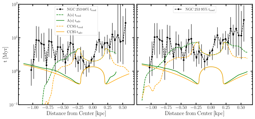
Figure 8: Left: Calculated cooling times for a 68% (black dashed line with ‘o’ markers). The solid orange line is the CC85 predicted advection time and the dashed orange line is the CC85 cooling time. The solid green line is the $A(s)$ predicted advection time and the dashed orange line is the $A(s)$ cooling time. Right: The same as the left but with the values for the 95% emission. We find that the cooling times for the 68% emission are of order the prediction advection times. This may indicate the presence of bulk radiative cooling in the outflow.

4.5 Mass Outflow Rates

We calculate an estimate of the outflow mass as $M=n_{e}m_{H}V/1.2f^{1/2}$ where the factor of 1.2 is from our assumed relation of $n_{e}=1.2n_{\rm H}$, $f$ is the filling factor which we assume 1, and $V$ is the cylindrical volume using a $95\%$ emission radius. We also calculate a mass outflow rate as $\dot{M}=n_{e}m_{H}rv/1.2f^{1/2}$ where $r$ is the vertical distance traveled, and $v$ is the outflow velocity. For $r$ we use 0.43 kpc in the northern and 0.95 kpc in the southern outflow, where we ignore the 200 pc central starburst region in order to solely capture the outflowing gas. For $v$ we assume a velocity of 1000 $\rm{km/s}$ based on the models described in Section 4.4. We find a mass in the northern outflow of $1.2\times 10^{6}\>M_{\odot}$ and a mass of $3.0\times 10^{6}\>M_{\odot}$ in the southern outflow. For the mass outflow rates with the assumptions from above, we find a rate of $2.8\>M_{\odot}/\rm{yr}$ in the northern outflow and $3.2\>M_{\odot}/\rm{yr}$ in the southern outflow.

We compare our mass outflow rate estimates with those from Strickland et al. (2000) and find that they are similar. Strickland et al. (2000) estimated a mass outflow rate upper limit of $2.2v_{3}\>M_{\odot}/\rm{yr}$ where $v_{3}$ is the outflow velocity in units of $3000\>\rm{km/s}$. Although the mass outflow rates are similar, the assumptions used in the estimates are different and warrant a discussion.

Strickland et al. (2000) used a velocity of 3000 km/s based on standard mass and energy injection rates from Leitherer & Heckman (1995). However, we find in our models described in Section 4.4, that the velocity profile produces much lower values. Based on our derived CC85 parameters of $\alpha_{95}\simeq 0.21$ and $\beta_{95}\simeq 0.36$, we find that the velocity of the wind is closer to 1000 km/s. Strickland et al. (2000) also used a filling factor of 0.4. They asserted than on scales of $\lesssim$ a few hundred parsecs, the pressures of the X-ray and H$\alpha$ emitting phase are similar. By equating their derived pressure (which they write in terms of the filling factor) to the H$\alpha$ pressure from McCarthy et al. (1987), they were able to derive a filling factor of 0.4.

If we use the Strickland et al. (2000) assumptions with our formulae, we find that the derived mass outflow rates are too large when compared to the cooler phases. Assuming $f=0.4$ and $v=3000$ km s^-1, we find a hot phase mass outflow rate of $13.5\>M_{\odot}/\rm{yr}$ in the northern outflow and $15.3\>M_{\odot}/\rm{yr}$ in the southern outflow. In the cool molecular phase, the estimate for the mass outflow rate is $14-39\>M_{\odot}/\rm{yr}$ (Krieger et al., 2019), while in the warm ionized phase, the mass outflow rate is $\approx 4\>M_{\odot}/\rm{yr}$ (Westmoquette et al., 2011; Krieger et al., 2019). The Strickland et al. (2000) assumptions would result in a hot phase outflow rate on par with the molecular phase rate and greater than the warm phase. The results from the Strickland et al. (2000) assumptions lead to mass outflow rates dominated by the hot phase.

4.6 Charge Exchange contribution

In order to acquire the most accurate measurements of outflow properties, the spectral model needs to include all the components that contribute significantly to the X-ray emission. Previous work has shown that charge exchange (CX), the stripping of an electron from a neutral atom by an ion, is one of these components. In particular, Lopez et al. (2020) found that when including CX in spectral models of the outflows of M82, CX contributes a significant portion (up to 25%) of the broad-band ($0.5-7$ keV) X-ray emission. Similarly, for several nearby star-forming galaxies (including NCC 253), Liu et al. (2012) showed that the K$\alpha$ triplet of He-like ions required a CX component to account for the observed line ratios. In the context of galactic winds, CX represents the emission of the hot phase interacting with the cooler phases where the hot ionized gas strips electrons from the cooler neutral gas.

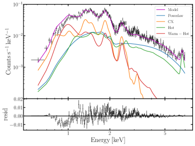
Figure 9: Spectra of the central region for Observation 20343 with the total spectral model, individual model components, and residuals plotted. The CX component accounts for significant fraction of spectra.

In our analysis, we find that three regions’ spectral fits were statistically significantly better, based on F-tests, with the inclusion of a CX component: the center and the two southern regions. At these locations, CX accounts for a significant fraction of the emission. As an example, in Figure 9 we show the spectra for Observation 20343 in the central region and note that CX makes up a significant fraction of the spectra. In the center region, the CX contribution is 42$\%$. For region S1, it is 20$\%$, and for region S2, it is 33$\%$ of the total broad-band X-ray emission. We note that the lack of a CX contribution in the northern outflow may be because of the high column density there, obscuring the soft X-rays necessary to distinguish the CX emission.

5 Conclusions

In this paper, we analyze $\approx$365 ks of archival Chandra data from NGC 253 to produce constraints on its starburst driven outflow that spans 1.1 kpc south and to 0.6 kpc north from the galaxy’s center. We extract spectra and use models to find the best-fit parameters ($kT$, $N^{\rm NGC253}_{\rm H}$, and metal abundances) in five regions along the outflow (Figure 3) and in nine regions of the galaxy’s disk (Figure 5).

With the exception of Ne which has a nearly flat distribution, the metal abundances peak in the galactic disk and decrease sharply along the minor axis (Figure 4 and Table 2). The distributions indicate significant dilution outside of the starburst region. For $kT$ and $N^{\rm NGC253}_{\rm H}$, the values also peak in the galactic disk and decrease along the minor axis. The decrease in abundances along the outflow may suggest mass loading or indicate other physics should be considered, such as non-equilibrium ionization.

We constrain the extent of the outflow in the regions and calculate $n_{e}$, pressure, and cooling times (Table 3). With these measurements we provide estimates of the hot phase mass outflow rates in Section 4.5, finding them to be $2.8\>M_{\odot}/\rm{yr}$ in the northern outflow and $3.2\>M_{\odot}/\rm{yr}$ in the southern outflow. We also find that the measured cooling times are of order the advection times predicted from models potentially indicating the presence of bulk radiative cooling in the outflow in Section 4.4. The models also show that incorporating non-spherical geometry provides a better match to observed $kT$ and $n_{e}$ profiles. We also find that the central region and southern outflow have significant contribution of $20-42$% to the broad-band X-ray emission from a CX component in Section 4.6.

In the future, expanding this approach to other starburst galaxies will reveal whether outflow properties vary with host galaxy properties, such as stellar mass. Chisholm et al. (2018) already showed that there is an inverse relationship between the metal loading factor and galaxy stellar mass in warm gas outflows. It would be worth investigating whether this relationship also holds in the hot phase, where most of the metals are being driven out.

Additionally, understanding of the hot gas in starburst-driven outflows will advance tremendously with the launch of XRISM (Tashiro et al., 2018). The mission will have higher spectral resolution, facilitating measurement of the hot wind velocity and enabling better constraints on the wind energy (Hodges-Kluck et al., 2019) and improving our hot phase mass outflow rate estimates.

References

- Arnaud (1996) Arnaud, K. A. 1996, in Astronomical Society of the Pacific Conference Series, Vol. 101, Astronomical Data Analysis Software and Systems V, ed. G. H. Jacoby & J. Barnes, 17
- Asplund et al. (2009) Asplund, M., Grevesse, N., Sauval, A. J., & Scott, P. 2009, ARA&A, 47, 481, doi: 10.1146/annurev.astro.46.060407.145222
- Bauer et al. (2007) Bauer, M., Pietsch, W., Trinchieri, G., et al. 2007, A&A, 467, 979, doi: 10.1051/0004-6361:20066340
- Beck et al. (2022) Beck, A., Lebouteiller, V., Madden, S. C., et al. 2022, A&A, 665, A85, doi: 10.1051/0004-6361/202243822
- Bendo et al. (2015) Bendo, G. J., Beswick, R. J., D’Cruze, M. J., et al. 2015, MNRAS, 450, L80, doi: 10.1093/mnrasl/slv053
- Bolatto et al. (2013) Bolatto, A. D., Warren, S. R., Leroy, A. K., et al. 2013, Nature, 499, 450, doi: 10.1038/nature12351
- Chevalier & Clegg (1985) Chevalier, R. A., & Clegg, A. W. 1985, Nature, 317, 44, doi: 10.1038/317044a0
- Chisholm et al. (2018) Chisholm, J., Tremonti, C., & Leitherer, C. 2018, MNRAS, 481, 1690, doi: 10.1093/mnras/sty2380
- Das et al. (2021) Das, S., Mathur, S., Gupta, A., & Krongold, Y. 2021, ApJ, 918, 83, doi: 10.3847/1538-4357/ac0e8e
- Das et al. (2019) Das, S., Mathur, S., Nicastro, F., & Krongold, Y. 2019, ApJ, 882, L23, doi: 10.3847/2041-8213/ab3b09
- de Vaucouleurs et al. (1991) de Vaucouleurs, G., de Vaucouleurs, A., Corwin, Herold G., J., et al. 1991, Third Reference Catalogue of Bright Galaxies
- Dere et al. (1997) Dere, K. P., Landi, E., Mason, H. E., Monsignori Fossi, B. C., & Young, P. R. 1997, A&AS, 125, 149, doi: 10.1051/aas:1997368
- Dickey & Lockman (1990) Dickey, J. M., & Lockman, F. J. 1990, ARA&A, 28, 215, doi: 10.1146/annurev.aa.28.090190.001243
- Fielding et al. (2017) Fielding, D., Quataert, E., McCourt, M., & Thompson, T. A. 2017, MNRAS, 466, 3810, doi: 10.1093/mnras/stw3326
- Finlator & Davé (2008) Finlator, K., & Davé, R. 2008, MNRAS, 385, 2181, doi: 10.1111/j.1365-2966.2008.12991.x
- Fruscione et al. (2006) Fruscione, A., McDowell, J. C., Allen, G. E., et al. 2006, in Society of Photo-Optical Instrumentation Engineers (SPIE) Conference Series, Vol. 6270, Society of Photo-Optical Instrumentation Engineers (SPIE) Conference Series, ed. D. R. Silva & R. E. Doxsey, 62701V, doi: 10.1117/12.671760
- Gupta et al. (2022) Gupta, A., Mathur, S., Kingsbury, J., Das, S., & Krongold, Y. 2022, arXiv e-prints, arXiv:2201.09915. https://arxiv.org/abs/2201.09915
- Hodges-Kluck et al. (2019) Hodges-Kluck, E., Lopez, L. A., Yukita, M., et al. 2019, BAAS, 51, 257. https://arxiv.org/abs/1903.09692
- Krieger et al. (2019) Krieger, N., Bolatto, A. D., Walter, F., et al. 2019, ApJ, 881, 43, doi: 10.3847/1538-4357/ab2d9c
- Lehmer et al. (2013) Lehmer, B. D., Wik, D. R., Hornschemeier, A. E., et al. 2013, ApJ, 771, 134, doi: 10.1088/0004-637X/771/2/134
- Lehnert & Heckman (1995) Lehnert, M. D., & Heckman, T. M. 1995, ApJS, 97, 89, doi: 10.1086/192137
- Leitherer & Heckman (1995) Leitherer, C., & Heckman, T. M. 1995, ApJS, 96, 9, doi: 10.1086/192112
- Leroy et al. (2015) Leroy, A. K., Bolatto, A. D., Ostriker, E. C., et al. 2015, ApJ, 801, 25, doi: 10.1088/0004-637X/801/1/25
- Leroy et al. (2021) Leroy, A. K., Schinnerer, E., Hughes, A., et al. 2021, ApJS, 257, 43, doi: 10.3847/1538-4365/ac17f3
- Levy et al. (2022) Levy, R. C., Bolatto, A. D., Leroy, A. K., et al. 2022, arXiv e-prints, arXiv:2206.04700. https://arxiv.org/abs/2206.04700
- Liu et al. (2012) Liu, J., Wang, Q. D., & Mao, S. 2012, MNRAS, 420, 3389, doi: 10.1111/j.1365-2966.2011.20263.x
- Lopez et al. (2020) Lopez, L. A., Mathur, S., Nguyen, D. D., Thompson, T. A., & Olivier, G. M. 2020, ApJ, 904, 152, doi: 10.3847/1538-4357/abc010
- McCarthy et al. (1987) McCarthy, P. J., van Breugel, W., & Heckman, T. 1987, AJ, 93, 264, doi: 10.1086/114309
- McCormick et al. (2013) McCormick, A., Veilleux, S., & Rupke, D. S. N. 2013, ApJ, 774, 126, doi: 10.1088/0004-637X/774/2/126
- Mills et al. (2021) Mills, E. A. C., Gorski, M., Emig, K. L., et al. 2021, ApJ, 919, 105, doi: 10.3847/1538-4357/ac0fe8
- Mitsuishi et al. (2013) Mitsuishi, I., Yamasaki, N. Y., & Takei, Y. 2013, PASJ, 65, 44, doi: 10.1093/pasj/65.2.44
- Müller-Sánchez et al. (2010) Müller-Sánchez, F., González-Martín, O., Fernández-Ontiveros, J. A., Acosta-Pulido, J. A., & Prieto, M. A. 2010, ApJ, 716, 1166, doi: 10.1088/0004-637X/716/2/1166
- Nguyen & Thompson (2021) Nguyen, D. D., & Thompson, T. A. 2021, MNRAS, 508, 5310, doi: 10.1093/mnras/stab2910
- Nguyen & Thompson (2022) —. 2022, ApJ, 935, L24, doi: 10.3847/2041-8213/ac86c3
- Oppenheimer & Davé (2008) Oppenheimer, B. D., & Davé, R. 2008, MNRAS, 387, 577, doi: 10.1111/j.1365-2966.2008.13280.x
- Ott et al. (2005) Ott, J., Weiss, A., Henkel, C., & Walter, F. 2005, ApJ, 629, 767, doi: 10.1086/431661
- Peeples & Shankar (2011) Peeples, M. S., & Shankar, F. 2011, MNRAS, 417, 2962, doi: 10.1111/j.1365-2966.2011.19456.x
- Plucinsky et al. (2018) Plucinsky, P. P., Bogdan, A., Marshall, H. L., & Tice, N. W. 2018, in Society of Photo-Optical Instrumentation Engineers (SPIE) Conference Series, Vol. 10699, Space Telescopes and Instrumentation 2018: Ultraviolet to Gamma Ray, ed. J.-W. A. den Herder, S. Nikzad, & K. Nakazawa, 106996B, doi: 10.1117/12.2312748
- Plucinsky et al. (2003) Plucinsky, P. P., Schulz, N. S., Marshall, H. L., et al. 2003, in Society of Photo-Optical Instrumentation Engineers (SPIE) Conference Series, Vol. 4851, X-Ray and Gamma-Ray Telescopes and Instruments for Astronomy., ed. J. E. Truemper & H. D. Tananbaum, 89–100, doi: 10.1117/12.461473
- Rekola et al. (2005) Rekola, R., Richer, M. G., McCall, M. L., et al. 2005, MNRAS, 361, 330, doi: 10.1111/j.1365-2966.2005.09166.x
- Rubin et al. (2014) Rubin, K. H. R., Prochaska, J. X., Koo, D. C., et al. 2014, ApJ, 794, 156, doi: 10.1088/0004-637X/794/2/156
- Silich et al. (2004) Silich, S., Tenorio-Tagle, G., & Rodríguez-González, A. 2004, ApJ, 610, 226, doi: 10.1086/421702
- Smith et al. (2012) Smith, R. K., Foster, A. R., & Brickhouse, N. S. 2012, Astronomische Nachrichten, 333, 301, doi: 10.1002/asna.201211673
- Strickland et al. (2000) Strickland, D. K., Heckman, T. M., Weaver, K. A., & Dahlem, M. 2000, AJ, 120, 2965, doi: 10.1086/316846
- Strickland et al. (2002) Strickland, D. K., Heckman, T. M., Weaver, K. A., Hoopes, C. G., & Dahlem, M. 2002, ApJ, 568, 689, doi: 10.1086/338889
- Tashiro et al. (2018) Tashiro, M., Maejima, H., Toda, K., et al. 2018, in Society of Photo-Optical Instrumentation Engineers (SPIE) Conference Series, Vol. 10699, Space Telescopes and Instrumentation 2018: Ultraviolet to Gamma Ray, ed. J.-W. A. den Herder, S. Nikzad, & K. Nakazawa, 1069922, doi: 10.1117/12.2309455
- Thompson et al. (2016) Thompson, T. A., Quataert, E., Zhang, D., & Weinberg, D. H. 2016, MNRAS, 455, 1830, doi: 10.1093/mnras/stv2428
- Veilleux et al. (2005) Veilleux, S., Cecil, G., & Bland-Hawthorn, J. 2005, ARA&A, 43, 769, doi: 10.1146/annurev.astro.43.072103.150610
- Veilleux et al. (2020) Veilleux, S., Maiolino, R., Bolatto, A. D., & Aalto, S. 2020, A&A Rev., 28, 2, doi: 10.1007/s00159-019-0121-9
- Verner et al. (1996) Verner, D. A., Ferland, G. J., Korista, K. T., & Yakovlev, D. G. 1996, ApJ, 465, 487, doi: 10.1086/177435
- Wang (1995) Wang, B. 1995, ApJ, 444, 590, doi: 10.1086/175633
- Wang & Liu (2012) Wang, Q. D., & Liu, J. 2012, Astronomische Nachrichten, 333, 373, doi: 10.1002/asna.201211657
- Westmoquette et al. (2011) Westmoquette, M. S., Smith, L. J., & Gallagher, J. S., I. 2011, MNRAS, 414, 3719, doi: 10.1111/j.1365-2966.2011.18675.x
- Wik et al. (2014) Wik, D. R., Lehmer, B. D., Hornschemeier, A. E., et al. 2014, ApJ, 797, 79, doi: 10.1088/0004-637X/797/2/79