Critical and near-critical relaxation of holographic superfluids

Abstract

We investigate the relaxation of holographic superfluids after quenches, when the end state is either tuned to be exactly at the critical point, or very close to it. By solving the bulk equations of motion numerically, we demonstrate that in the former case the system exhibits a power law falloff as well as an emergent discrete scale invariance. The later case is in the regime dominated by critical slowing down, and we show that there is an intermediate time-range before the onset of late time exponential falloff, where the system behaves similarly to the critical point with its power law falloff. We further postulate a phenomenological Gross–Pitaevskii-like equation that is able to make quantitative predictions for the behavior of the holographic superfluid after near-critical quenches. Intriguingly, all parameters of our phenomenological equation which describes the non-linear time evolution may be fixed with information from the static equilibrium solutions and linear response theory.

1 Introduction

So-called holographic superconductors have been a steady source of inspiration and target of research for the holography community since their inception in Hartnoll:2008vx ; Hartnoll:2008kx ; Herzog:2008he ; Herzog:2009xv ; Gubser:2008px . Despite the established nomenclature, it is commonly understood that these systems might more correctly be understood to be holographic superfluids, because the gauge-symmetry present in the bulk should translate into a global symmetry according to common AdS/CFT wisdom.

However, it has been demonstrated in Domenech:2010nf that the Maxwell equations on the boundary can be imposed, leading to a genuine holographic superconductor. Another interesting perspective was offered in Maeda:2010br , where it was argued that we should understand large gauge transformations in the bulk to give rise to transformations that can be interpreted as ”background-gauge” transformations in the boundary theory, affecting the sources imposed there but not being tied to a dynamical photon. This perspective will be especially influential for our work.

The goal of this work is to study how holographic superconductors relax to their equilibrium state after a quench when the final state is close to the critical point. Generically, for a near-critical end-state this relaxation will of course be characterized at late times by an exponential falloff, where the half-life time of said falloff diverges as the end-state is taken towards the critical point. This is known as critical slowing down RevModPhys.49.435 , see Maeda:2008hn ; Maeda:2009wv ; Natsuume:2010vb ; Ewerz:2014tua for works in the holographic context.

But what happens when the end-state is tuned to lie exactly at the critical point? In this case, the exponential falloff behavior is replaced by a power law falloff PhysRevB.96.054303 ; PhysRevB.81.012303 . This makes sense intuitively, because a power law falls off slower than any exponential, hence this is a physically sensible result in the limit where the half-life time diverges. From the holographic bulk perspective this may be seen as the system trying to balance the condensate floating above the horizon exactly, hence the slow decay. The condensate is affected by electrostatic forces driving it into the bulk and gravitational forces trying to pull it into the horizon Gubser:2008wv . In the following, we will study such critical and near-critical quenches both from the bulk and the boundary perspective. Note, however, that unlike in the discussion about the Kibble-Zurek mechanism Chesler:2014gya ; Sonner:2014tca ; Bhaseen:2012gg ; delCampo:2021rak ; Li:2021jqk we are interested in quenches with initial state in the ordered phase, i.e. the quenches we are studying do not cross the critical point at any finite rate.

2 Bulk results

We consider the common bulk gravitational model of a superconductor in AdS₄/CFT₃ Hartnoll:2008vx ; Hartnoll:2008kx ; Herzog:2008he

$$S\,=\,S_{\text{grav}}+\frac{1}{2\kappa^{2}}\int_{\mathcal{M}}\mathrm{d}^{4}x\,\sqrt{-g}\left[-\frac{1}{4\,q^{2}}F_{\mu\nu}F^{\mu\nu}-|D\varphi|^{2}-m^{2}|\varphi|^{2}\right]+S_{\text{nf}}\,.$$ (1)

The field content consists of the metric field $g_{\mu\nu}$, a $U(1)$ gauge field $A_{\mu}$ ($F=dA$) and a complex scalar field $\varphi$ of mass $m^{2}=-2$ charged under the gauge field with $D_{\mu}\equiv\partial_{\mu}-i\,q\,A_{\mu}$ with charge $q=+1$. We will neglect backreaction in this work, and hence fix the metric

$$\mathrm{d}s^{2}=\frac{1}{u^{2}}\left[-f(u)\,\mathrm{d}t^{2}-2\,\mathrm{d}t\mathrm{d}u+\mathrm{d}x^{2}+\mathrm{d}y^{2}\right],$$ (2)

with $f(u)=1-u^{3}$ where we already set $u_{h}=1$ and $L=1$. We measure all physical quantities in terms of the fixed temperature $\bar{T}=4\pi T/3$ where $T=|f^{\prime}(1)|/(4\pi)$. To keep the notation simple we assume that all appearing quantities have already been divided by the appropriate power of $\bar{T}$ and hence are dimensionless. $S_{\text{nf}}$ is interpreted as an external source which we use to perform a quench in the charge density. The equations of motion (eoms) are solved by a fully pseudo-spectral code (in space and time) as previously employed in Ammon:2016fru . See appendix A for more details on this setup (including $S_{\text{nf}}$) and the numerical methods used to solve it.

The near boundary expansions of the bulk matter fields read

$$\varphi \sim\langle\mathcal{O}\rangle u^{2}+\ldots,$$ (3)

$$A_{t} \sim\mathcal{A}_{t}-\rho u+\ldots,$$ (4)

where we set the source of the scalar field to zero in order to engineer spontaneous symmetry breaking and $2\kappa^{2}\langle\mathcal{O}\rangle\equiv\Psi(t)=\phi(t)e^{i\psi(t)}$ is the complex expectation value of the dual operator Arean:2021tks . At static equilibrium we identify $\mathcal{A}_{t}=\mu$ where $\mu$ is the chemical potential. The subleading component $\rho(t)$ is the charge density. There is a second order phase transition to a phase with non-zero condensate at $\rho=\rho_{c}\approx 4.06371$. We perform quenches of the system by giving $\rho$ a step-function-like time dependence. See appendix A.2 for more details.

Some of our numerical results are shown in figure 1. It is clear that we observe late time power-law falloffs in $\phi(t)$, $|\dot{\psi}(t)|$, and $|\mathcal{A}_{t}(t)-\rho_{c}|$ that are universal, i.e. independent on the initial state or other details of the quench. At late times, where $\rho$ is held constant in time, the bulk equations of motion are not explicitly dependent on $t$, and so for any collective solution $y(t)$ of the bulk eoms, $y(t+\delta t)$ will also be a solution for any $\delta t$. We hence make an ansatz of the form

$$\phi(t) =A(t+\delta t)^{\alpha}$$ (5)

$$\dot{\psi}(t)-(\mathcal{A}_{t}(t)-\rho_{c}) =B(t+\delta t)^{\gamma}$$ (6)

which we fit to our numerical curves at late times ($t\geq 5\times 10^{4}$). We only consider the combination on the left hand side of equation (6) because it is gauge invariant under background-gauge transformations Maeda:2010br . With a high degree of consistency between the five different quenches plotted in figure 1, we obtain

(9)

with only the value of $\delta t$ obtained from the fit varying significantly from quench to quench.

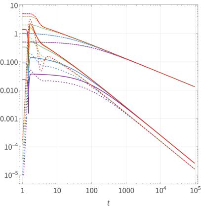
Figure 1: Numerical results for $|\mathcal{A}_{t}(t)-\rho_{c}|$ (solid lines), $|\langle\mathcal{O}\rangle|\equiv\phi(t)$ (dashed lines), and $|\dot{\psi}(t)|$ (dotted lines) for multiple exactly critical quenches starting from $\rho_{\text{initial}}=\{4.124,4.302,4.951,6.981,8.184\}$ (purple, blue, green, orange, red). We clearly observe a universal power-law like late time behavior with $\phi\propto 1/\sqrt{t}$ and $|\mathcal{A}_{t}-\rho_{c}|,|\dot{\psi}|\propto 1/t$.

The observed behavior $|\dot{\psi}|\propto 1/t$ indicates $\psi(t)\propto\log{t}$, i.e. oscillations of the real- and imaginary part of $|\langle\mathcal{O}\rangle|$ that are periodic on a logarithmic time axis. This signifies the presence of a discrete scale invariance, in contrast to the continuous scale invariance inherent to ordinary power laws SORNETTE1998239 . Among other contexts, such discrete scale invariance has also previously been observed numerically after critical quenches in a holographic Kondo model in Erdmenger:2016msd , as well as in the formation of black holes through the collapse of charged scalar fields PhysRevD.51.4198 .

3 Boundary model

From a boundary point of view, it is of course known that the phenomenology of superconductors is well-described by the (complex) Ginzburg–Landau equation, while for superfluids with their global symmetry breaking the Gross–Pitaevskii equation takes a similar role RevModPhys.74.99 ; tsuneto_1998 . Consequently, there has been some recent activity in PhysRevLett.127.101601 ; Yan:2022jfc trying to fit parameters of Gross–Pitaevskii equations in order to model aspects of the non-equilibrium behavior of holographic superfluids.

Unlike the quenches that we study in this manuscript, PhysRevLett.127.101601 ; Yan:2022jfc investigated inhomogeneous setups where space-derivatives are non-zero which increases the complexity of the problem significantly. In addition, in our paper we explicitly aim to study behavior near or even exactly at the critical point which means that our results should be ideally suited for such a phenomenological description, since e.g. the Ginzburg-Landau equation is usually seen as a series expansion around vanishing order-parameter, where higher order terms in the free energy are dropped.

We now postulate the phenomenological equation

$$\left[\partial_{t}-iC_{1}\left(\mathcal{A}_{t}(t)-\rho+C_{5}|\Psi(t)|^{2}\right)\right]\Psi(t)\equiv-(C_{2}+iC_{3})\left[|\Psi(t)|^{2}-C_{4}(\rho-\rho_{c})\right]\Psi(t),$$ (10)

where again $\Psi=\phi e^{i\psi}$, $\rho,\rho_{c},\psi,\mathcal{A}_{t},C_{i}\in\mathbb{R}$, $\phi>0$, and we manifestly neglect any terms including spatial derivatives or higher orders of $\Psi$ or $\rho-\rho_{c}$. The parameter $\rho$ is assumed to be constant in time, and $C_{1}$ is merely the charge of the complex field which in our case has the value $+1$.

The right hand side of the equation is similar to the variation of the free energy that would appear in the Ginzburg-Landau equation, multiplied with a complex prefactor which is inspired by the dissipative Gross-Pitaevski equations used in PhysRevLett.127.101601 ; Yan:2022jfc , see also RevModPhys.74.99 ; doi:10.1137/0142054 . The left hand side is essentially a gauge-covariant time-derivative plus some extra terms whose relevance will become clear shortly. The gauge covariance is necessary in order to respect the background gauge-invariance (without dynamical photon) described in Maeda:2010br which arises as a consequence of large gauge transformations which do not fall off towards the boundary and hence change the boundary values of the bulk fields such as $\mathcal{A}_{t}$.

Because (10) contains complex factors, we can split it into a real and imaginary part when trying to solve it (after dividing by $e^{i\psi}$ on both sides). Besides the trivial case $\phi=0$ which we will ignore, the real part of this equation only depends on $\phi(t)$ and has the non-trivial exact solution

$$\phi(t)=\sqrt{\frac{C_{4}(\rho-\rho_{c})}{1-\left(1-\frac{C_{4}(\rho-\rho_{c})}{\phi_{0}^{2}}\right)e^{-2C_{2}C_{4}t(\rho-\rho_{c})}}}$$ (11)

with $\phi(0)=\phi_{0}$. This solution can then be plugged into the imaginary part of (10) in order to obtain an algebraic equation that can be solved for the gauge-invariant expression $\dot{\psi}-C_{1}\mathcal{A}_{t}$ (see appendix B). Obtaining a unique solution for both $\psi(t)$ and $\mathcal{A}_{t}(t)$ requires some kind of gauge fixing condition.

As a simple consistency check, looking for non-trivial ($\phi\neq 0$) static solutions yields

$$\phi =\sqrt{C_{4}(\rho-\rho_{c})}$$ (12)

$$\mathcal{A}_{t} =\rho-C_{5}\phi^{2}$$ (13)

$$=\text{$\rho$}-C_{4}C_{5}(\rho-\rho_{c})$$ (14)

when $C_{4}(\rho-\rho_{c})>0$, i.e. we observe the expected formation of the superfluid phase, and the deviation of the chemical potential $\mu=\mathcal{A}_{t}$ from its value $\mu=\rho$ in the normal phase.

In the non-equilibrium case, the late time behavior of (11) and the more cumbersome solution for $\dot{\psi}-C_{1}\mathcal{A}_{t}$ depend crucially on whether we are in the superfluid phase where

$$\phi(t)-\sqrt{C_{4}(\rho-\rho_{c})}\propto e^{-2C_{2}C_{4}(\rho-\rho_{c})t}+...$$ (15)

or in the normal phase where

$$\phi(t)\propto e^{C_{2}C_{4}(\rho-\rho_{c})t}+...\ .$$ (16)

The crucial insight is that we can determine the phenomenological parameters $C_{i}$ by comparing our results so far to the properties of the static solution in the superfluid phase and the late time quasinormal mode like falloff towards this static solution after a non-critical quench. As explained in appendix B, this allows to numerically fix the parameters (normalized to $\bar{T}$) of the model to

$$\begin{tabular}[]{lllllll}$C_{2}$&$\approx$&0.03018&$C_{3}$&$\approx$&0.09308\\ $C_{4}$&$\approx$&4.09192&$C_{5}$&$\approx$&0.14967\end{tabular}\ .$$ (19)

Once this determination has been made, the model (10) is able to make predictions for the behavior of the system at earlier times after a non-critical quench (via the full expression (11)) as well as the exactly critical quenches where at late times $\rho=\rho_{c}$. Let’s consider the latter case first. In this limit, (11) simplifies to

$$\phi(t)=\frac{1}{\sqrt{2C_{2}t+\frac{1}{\phi_{0}^{2}}}}\approx\frac{4.07}{t^{1/2}}+...$$ (20)

and additionally we find

$$\dot{\psi}-C_{1}(\mathcal{A}_{t}-\rho_{c})=\frac{C_{1}C_{5}+C_{3}}{2C_{2}t+\frac{1}{\phi_{0}^{2}}}\approx\frac{0.94}{t}+...\ .$$ (21)

Even though these quantities will be small at late times, it is important to note that these solutions depend on the non-linear features of equation (10) and could not be obtained through a linearized ansatz. Comparing the predictions (20) and (21) with our results given in equations (5), (6), and (9), we find excellent agreement.

Let us now return to the issue of near-critical quenches, by which we mean quenches that both start and end near the critical point, but not exactly at it. We know that at very late times, after such a quench the system will be characterized by an exponential falloff towards the new equilibrium, however via the solution (11), equation (10) allows us to describe the behavior of the system already at much earlier times. A representative example of a near-critical quench is depicted in figure 2. In the curve for $\phi(t)$, we can see that before the equilibrium is reached at very late times, there is a long intermediate stretch of time in which the condensate appears to fall off in a power law-like manner. In particular, after a quench that brings the system infinitesimally close to the critical point, the system will initially react as if it was relaxing exactly to the critical point, and only after what we call ”handover-timescale”

$$t_{\text{ho}}\sim\frac{1}{\rho-\rho_{c}}$$ (22)

the system will notice that it is not at the critical point, and the power-law behavior gives way to an exponential falloff towards a small but finite condensate. Of course, this handover timescale is identical to the relaxation timescale of the system close to the critical point. This phenomenological behavior is exactly encapsulated in equation (11), see also appendix B and appendix C for further information.

As the parameters $C_{i}$ are given in (19) and the value $\rho$ is determined by the choice of quench, the only parameter that needs to be determined in order to compare our analytical prediction with the numerical result is $\phi_{0}$. We could hence use (11) as a model with one free parameter that needs to be fitted to the data. However, as we can see in figure 2, in contrast to $\dot{\psi}-\mathcal{A}_{t}$, $\phi(t)$ does not change significantly during and immediately after the quench. Neither would a sudden change be predicted by (11). Hence, as we know the initial state before the quench exactly, we can simply set $\phi_{0}\equiv\phi(0)$, even though formally equations (10) and (11) only become valid after the quench, when $\rho$ is constant. As can be seen in figure 2, this trick is sufficient to obtain a very good match between numerical data and analytical solution.

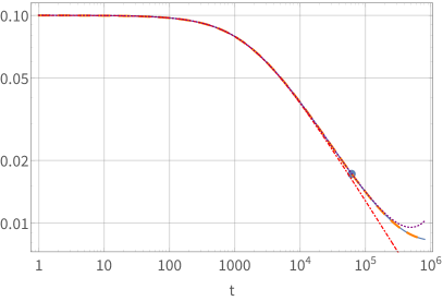
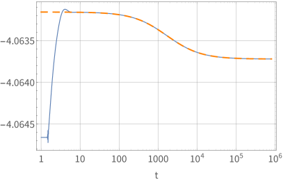
Figure 2: Comparison between numerical (solid blue) and analytical (dashed orange) results for a near-critical quench, with $\rho_{\text{initial}}=$4.06626 and $\rho_{\text{final}}=$4.06373. The top frame shows $\phi(t)$, while the bottom frame shows $\dot{\psi}(t)-C_{1}\mathcal{A}_{t}(t)$. For the times after the quench ($t\gtrsim 10$), numerical and analytical curves agree very well. The dot signifies the handover-time scale (22), while the dash-dotted red line shows the critical solution (20). The dotted purple line shows the approximation $\phi(t)\approx(2C_{2}t+1/\phi_{o}^{2})^{-1/2}e^{C_{4}(\rho-\rho_{c})(2C_{2}t+1/\phi_{0}^{2})/4}$ derived in appendix C.

4 Discussion

In this paper, we have studied the relaxation of a holographic superconductor close or exactly at the critical point, both from a bulk and a boundary perspective.

In the bulk, our methods of choice were extensive numerical simulations over long ranges of time. We demonstrated that for critical quenches, in addition to the expected power law falloff of the modulus $|\langle\mathcal{O}\rangle|$ of the order parameter, its complex phase undergoes rotations which are periodic on a logarithmic time axis, leading to a discrete scale invariance of the solution. Furthermore, we observed that the power law falloff characteristic for the critical quenches is approximately observable even in the non-critical quenches for an intermediate time-period before the onset of the late-time exponential falloff at a handover-timescale (22).

On the field theory side, we postulated a phenomenological Gross–Pitaevskii-like equation to describe the behavior of the system. This equation can be solved analytically, and its parameters can be fixed by comparing to the numerical data on the late-time exponential falloff after non-critical quenches. In particular, we can fix the parameters of the equation with information about the static equilibrium states and linearized fluctuations about them (quasinormal modes (QNMs)) which are computationally much easier to obtain than the non-linear time evolution. The constants obtained from the QNM data in the superfluid and normal fluid phase match which is a non-trivial check of our suggested equation (10). In our study we also successfully applied and tested a novel concept about computing the amplitudes of QNM excitations developed in Arean:2021tks leading also to some novel insights about the linear response behavior.

Once the parameters are fixed, the phenomenological equation allows to predict with good accuracy both the behavior after exactly critical quenches, as well as the behavior after near-critical quenches for intermediate time-scales. It should be pointed out that both in the bulk and on the boundary, our results are intimately tied to the non-linearities of the respective equations of motion, and could not be studied with a simple linearized ansatz. Interestingly, the papers Mitman:2022qdl ; Cheung:2022rbm have recently commented on the limitations of linearized ansätze in the study of black hole ringdowns.

There are multiple possible directions for further research. Three obvious generalisations would be to include a possible $x$-dependence (similar to PhysRevLett.127.101601 ; Yan:2022jfc ; Adams:2012pj ; Sonner:2014tca ), to study holographic superconductors in different dimensions, and to turn on backreaction on the metric in the bulk. Preliminary results indicate the possibility to generalize our phenomenological equation (10) to a finite rate of superflow within the parameter regime of second order phase transitions up to the tricritical point. We hope to revisit these ideas in a future publication.

Appendix A Numerical methods

In this section, we give a brief overview of the numerical methods used to solve the partial differential equations numerically.

Within numerical holography, pseudo-spectral methods are widely applied to find highly accurate solutions to boundary value problems in terms of elliptic partial differential equations or ordinary differential equations. However, for initial value problems of hyperbolic partial differential equations space and time are typically treated differently. The spatial dependence is usually discretized by means of a (pseudo)-spectral method which is combined with an explicit 4th order Runge-Kutta scheme or Adams-Bashforth method to evolve the solution in time Chesler:2013lia . Within a fully spectral scheme, we discretize time and space with (pseudo)-spectral methods yielding a highly implicit and accurate time evolver.

The basic idea of (pseudo)-spectral methods Boyd1989ChebyshevAF  is that the unknown functions $u(x)$ which is the solution to the differential equation

$$\mathcal{L}_{x}u(x)=g(x),$$ (23)

where $\mathcal{L}_{x}$ is a differential operator, may be approximated by a finite number $N$ of basis polynomials $\phi_{i}(x)$

$$u(x)\approx u_{N}(x)=\sum_{i=0}^{N-1}c_{i}\phi_{i}(x).$$ (24)

To find the solution, we require that the residuum $R=\mathcal{L}_{x}u_{N}-g$ vanishes exactly on the chosen set of discrete grid points. Note that for the exact solution, the residuum vanishes identically. For a given choice of grid points and basis polynomials, the derivatives are replaced by discrete matrices acting on the whole domain.

Fully spectral algorithms have been employed within (asymptotically flat) numerical relativity in Hennig:2008af ; Hennig:2012zx ; Petri2014ASM ; PanossoMacedo:2014dnr ; Hennig:2020rns and in the context of holography in Ammon:2016fru ; Grieninger:2016xue . Let us outline the recipe for our numerical algorithm (see also the appendix of Grieninger:2016xue ).

A.1 Numerical algorithm

We are looking for a solution at time $t=t_{\text{final}}$ to the initial value problem at $t=t_{\text{initial}}$.

1. At $t=t_{\text{initial}}$, we may obtain the initial configuration by solving the static set of ordinary differential equations subject to the boundary conditions $\varphi^{\prime}(t_{\text{initial}},0)=0$ and $\varphi^{\prime\prime}(t_{\text{initial}},0)=|\langle\mathcal{O}_{\text{initial}}\rangle|$ and $A_{t}(t_{\text{initial}},1)=0$. As discretization of the radial direction $u\in[0,1]$, we chose Gauss-Lobatto grid points $u_{j}=\frac{1}{2}\left(1+\cos(\pi j/N_{u})\right)$, where $j\in[0,N_{u}-1]$.

2. To evolve in time, we decompose the time interval $(t_{\text{initial}},t_{\text{final}}]=(t_{\text{initial}},t_{1}]\cup(t_{1},t_{2}]\cup...\cup(t_{p},t_{\text{final}}]$ in $p+1$ subintervals in the spirit of multi-domain decompositions. Note that the different time intervals may have different sizes which we set by a adaptive step control depending on how much the solution changes on the interval.

3. For a given initial solution, we introduce auxiliary functions
   $h(t,u)=h_{\text{in}}(t=t_{i},u)+(t-t_{i})\,h_{\text{aux}}(t,u)$ on each subinterval $(t_{i},t_{j}],\,t_{j}>t_{i}$.

4. The radial coordinate is discretized by the Chebyshev-Lobatto (CL) grid and to discretize the time coordinate, we chose a right-sided Chebyshev-Radau (rCR) grid (for some generic time interval $t\in(t_{i},t_{j}]$)

   $$u_{j}=\frac{1}{2}\left(1+\cos\left(\frac{\pi j}{N_{u}}\right)\right),$$ (25)

   $$t_{k}=\frac{1}{2}\left[(t_{j}-t_{i})+(t_{j}-t_{i})\cos\left(\frac{2\pi k}{2N_{t}+1}\right)\right],$$ (26)

   where $j=0,\ldots,N_{u}-1$, and $k=0,\ldots,N_{t}$. Note that the right-sided Chebychev-Radau grid does not include the initial slice of the interval where we already know the solution.

5. Replace all derivatives by their discrete versions given by the derivative matrices $D$: $\partial_{u}\to D^{\text{CL}},\partial_{t}\to D^{\text{rCR}}$ and discretize the equations of motion on the square spanned by the discrete spectral coordinates and impose the desired boundary.

6. Solve the corresponding non-linear system with a Newton-Raphson method.

7. Use the solution on the final slice $t_{j}$ as new initial solution in the next step.

Typically, we use $N_{u}=40$ or $N_{u}=50$ in combination with $N_{t}=14$. We monitored that the constraint equation is satisfied better than $10^{-15}$ during the time evolution. Note that we additionally fix $A_{t}(t,1)=0$. The numerical algorithm is implemented in Mathematica.

The numerical methods used to compute the initial configurations, background solutions and QNMs are the same codes as used in Ammon:2021pyz .

A.2 Quench profiles

For spontaneous $U(1)$ symmetry breaking, charge conservation imposes $\dot{\rho}(t)=0$ in the absence of external sources. However, our goal is to study quenches from the superfluid phase with $\rho=\rho_{\text{initial}}$ to the critical point $\rho=\rho_{\text{crit}}$ (or close to it for some $\rho=\rho_{\text{final}}$). Since we work in the probe limit, we have to introduce an external source in order to change $\rho$ to our desired final value. We could achieve this by breaking the $U(1)$ explicitly with a scalar source as done in Bhaseen:2012gg , or we consider some generic external source that changes $\rho$ directly by considering the null fluid (nf) current Fernandez-Pendas:2019rkh

$$2\kappa^{2}\,J_{(\text{nf})}^{u}=\frac{\dot{\rho}}{\sqrt{-g}}.$$ (27)

which may be achieved by coupling

$$S_{\text{nf}}=\int_{\mathcal{M}}dx^{4}\sqrt{-g}A_{\mu}j^{\mu}_{\text{ext}}\,,$$ (28)

to the action. This leads to a covariantly conserved external current

$$j_{\text{ext}}^{\mu}=\dfrac{\dot{\rho}}{\sqrt{-g}}\delta^{\mu}_{u}\,.$$ (29)

which allows us to change the electric charge at will. Technically, the external source also drives the $T^{tt}$ component of the energy-momentum tensor. However, in the large $q$ expansion of the probe limit this contribution is subleading and we can neglect it similarly to the backreaction of the matter fields onto the geometry.

To quench our system, we chose to manipulate $\rho$ with the external source and quench it to its final value. Note that in the late time behavior, the external source is switched off and we verified that the late time behavior is independent of the quench profile. Concretely, we performed quenches with

$$\rho(t)=\rho_{\text{initial}}+\frac{1}{2}(\rho_{\text{final}}-\rho_{\text{initial}})(1+\tanh[\Omega(t-t_{s})]);$$ (30)

where $\Omega=10$ is the rapidity and $t_{s}=1.5$ is the center of the quench.

Appendix B Determination of parameters

The parameters $C_{4},C_{5}$ of equation (10) can be determined by fitting equations (12),(14) to the behavior of the static holographic superconductor close to the critical point. One way to determine $C_{2},C_{3}$ is to compare the predicted late time behavior after a non-critical quench into the superfluid phase to numerical data of the non-linear time evolution. With the parameters fixed in this way, (10) then allows to make genuine predictions for both exactly critical quenches, and for the behavior of non-critical quenches at early and intermediate times.

Giving some more details than in eq. (15), we find that for $t\gg 1$, quenches in the superfluid phase will relax as

$$\phi(t)=\sqrt{C_{4}}\sqrt{\rho-\rho_{c}}+\frac{\sqrt{C_{4}}}{2}\sqrt{\rho-\rho_{c}}\left(1-\frac{C_{4}(\rho-\rho_{c})}{\phi_{0}^{2}}\right)e^{-2C_{2}C_{4}t(\rho-\rho_{c})}+...$$ (31)

$$\dot{\psi}(t)-C_{1}\mathcal{A}_{t}(t)= -C_{1}\rho+C_{1}C_{4}C_{5}(\rho-\rho_{c})$$

$$-\frac{C_{4}(C_{1}C_{5}-C_{3})}{\phi_{0}^{2}}\left(C_{4}(\rho-\rho_{c})-\phi_{0}^{2}\right)(\rho-\rho_{c})e^{-2C_{2}C_{4}t(\rho-\rho_{c})}+...$$ (32)

while in the normal phase we would find

$$\phi(t)=\sqrt{\frac{C_{4}(\rho_{c}-\rho)}{1-\frac{C_{4}(\rho-\rho_{c})}{\phi_{0}^{2}}}}e^{-C_{2}C_{4}t(\rho_{c}-\rho)}+...$$ (33)

$$\dot{\psi}(t)-C_{1}\mathcal{A}_{t}(t)=-C_{1}\rho+C_{3}C_{4}(\rho-\rho_{c})+\frac{C_{4}\phi_{0}^{2}(\rho-\rho_{c})(C_{1}C_{5}-C_{3})}{C_{4}(\rho-\rho_{c})-\phi_{0}^{2}}e^{-2C_{2}C_{4}t(\rho_{c}-\rho)}+...\ .$$ (34)

Clearly, $C_{2}$ can be determined by fitting the half-life time of the predicted late time exponential falloff in the superfluid phase to the numerical data of the non-linear time evolution. The amplitude of this exponential falloff itself is of course dependent on $\phi_{0}$ for each of these functions, however the ratio between the amplitudes

$$\frac{\text{Amplitude}_{\phi}}{\text{Amplitude}_{\dot{\psi}(t)-C_{1}\mathcal{A}_{t}(t)}}=\frac{1}{2\sqrt{C_{4}(\rho-\rho_{c})}}\frac{1}{C_{1}C_{5}-C_{3}}$$ (35)

is independent of $\phi_{0}$ and can be used to obtain a unique value of $C_{3}$.

However, it is not necessary to perform the non-linear time evolution to fit the constants (19). In the following, we explain how all of them may be obtained within linear response theory and from the static solutions in the context of holography. The two constants $C_{4}$ and $C_{5}$ may simply be obtained by constructing the static solutions near the phase transition and fit the condensate and chemical potential, respectively, to the deviation of $\rho$ from its critical value $\rho_{c}$ according to eqs. (12) and (14). The constant $C_{2}$ may be obtained from the QNMs at zero wavevector in the superfluid phase (15) or in the normal phase (16). To probe the QNMs we consider linearized fluctuations of a complex scalar $\delta\bar{\Psi}=\delta\Psi e^{-i\omega t}$ and the gauge field $\delta\bar{a}_{t}=\delta a_{t}e^{-i\omega t}$. Note that we may decompose the scalar fluctuations about a state with zero background phase according to $(\langle\mathcal{O}_{\text{eq}}\rangle+\langle\delta\mathcal{O}\rangle)e^{i\delta\psi}=(\langle\mathcal{O}_{\text{eq}}\rangle+\langle\delta\mathcal{O}\rangle)(1+i\delta\psi)=(\langle\mathcal{O}_{\text{eq}}\rangle+\text{Re}(\delta\Psi)+i\,\text{Im}(\delta\bar{\Psi})$, with $\text{Re}(\delta\Psi)=\langle\delta\mathcal{O}\rangle)$ and $\text{Im}(\delta\bar{\Psi})=\langle\mathcal{O}_{\text{eq}}\rangle\,\delta\psi$.

Let us focus on the normal phase first and consider linearized solutions about the static normal phase solution with $\langle\mathcal{O}\rangle=0,\,\rho<\rho_{c}$. The corresponding QNM responsible for the relaxation to equilibrium is the pair of massive scalar modes. Close to the phase transition the QNMs in the normal phase behave (to lowest order in $\rho-\rho_{c}$) like

$$\omega_{\pm}=-(\pm 0.38087-0.12348i)\,(\rho-\rho_{c})$$ (36)

According to eq. (16), we can read of the constant $C_{2}$ (since we already know $C_{4}$ from the static solution) from the imaginary part of the QNM (36) leading to the value indicated in (19). Similarly, the real part determines the constant $C_{3}=-\text{Re}(\omega_{+})/C_{4}$ as may be seen from eq.(34). Since the QNM comes as a pair, the sign is seemingly not determined. However, it is possible to reconstruct which sign belongs to fluctuations of $\delta\Psi$ and $\delta\bar{\Psi}$. In order to determine the QNMs we solve the fluctuation equations as generalized eigenvalue problem of the form $(\bm{A}\omega-\bm{B})\,\bm{x}=0$, where $\bm{A}$ and $\bm{B}$ are differential operators of a non-hermitian Sturm-Liouville problem (see Arean:2021tks for more details). Usually, only the eigenvalues $\omega$ are of interest since they correspond to the QNM frequencies. However, it is also possible to examine the eigenvector $\bm{x}$ corresponding to the eigenvalue $\omega$. In our case, we observe that fluctuations with $\omega=\omega_{+}$ are carried by $\bm{x}=\{\delta\Psi,0\}$ while $\omega=\omega_{-}$ is carried by $\bm{x}=\{0,\delta\bar{\Psi}\}$.

As an independent, non-trivial check of our proposed equation, we now compute the constants $C_{2}$ and $C_{3}$ from the QNMs in the superfluid phase. To compute $C_{3}$, we need information about the relative amplitudes of the fluctuations supporting the QNM responsible for equilibration. Only recently, the authors of Arean:2021tks suggested a method to compute the relative contributions of boundary operators to a certain QNM excitation from the aforementioned eigenvectors. Here, we want to dissect the so called “amplitude” or Higgs mode. At zero wave vector, this pseudo-diffusive mode is driving the system to equilibrium in the superfluid phase Amado:2013xya . More recently, the dynamics of this mode was discussed in terms of a linearized bulk analysis in Donos:2022xfd . Close to equilibrium, we find for the QNM frequency to lowest order in $\rho-\rho_{c}$ (and at zero wave vector)

$$\omega_{\text{Ampl}}=-0.2469\,i\,(\rho-\rho_{c}).$$ (37)

According to eq. (16), we may extract $C_{2}$ from this information leading to the same numerical value as computed in the normal phase. Employing the techniques developed in Arean:2021tks , we can extract the expectation values of the operators carrying this QNM excitation from the corresponding eigenvector. Intriguingly, we find that the gauge fluctuations have expectation value zero and the mode is solely carried by the scalar fluctuations. Close to the critical point we thus find to lowest order in $\rho-\rho_{c}$ (and at zero wave vector) that

$$\frac{\text{Amplitude}_{\langle\delta\mathcal{O}\rangle}}{\text{Amplitude}_{\langle\delta\dot{\psi}\rangle-\langle\delta a_{t}\rangle}}=\frac{17.67}{2\,\sqrt{C_{4}(\rho-\rho_{c})}}.$$ (38)

Once $C_{5}$ is fixed from the background data, eq. (38) determines the value of $C_{3}$ in accordance with our data from the normal phase. Note that this is a non-trivial and independent check of the numerical values we obtained for $C_{2}$ and $C_{3}$ thus confirming the prediction of our suggested model.

Appendix C Analysis of intermediate time behavior

We will now give an analysis of the behavior at intermediate time scales predicted by the solution (11) as well as the corresponding solution

$$\dot{\psi}-C_{1}\mathcal{A}_{t}=-C_{1}\rho-C_{3}C_{4}(\rho-\rho_{c})+\frac{C_{4}(C_{3}+C_{1}C_{5})(\rho-\rho_{c})}{1-e^{-2C_{2}C_{4}t(\rho-\rho_{c})}\left(1-\frac{C_{4}(\rho-\rho_{c})}{\phi_{0}^{2}}\right)}.$$ (39)

First of all, we notice that $\frac{C_{4}(\rho-\rho_{c})}{\phi_{0}^{2}}=\frac{\phi(t\rightarrow\infty)^{2}}{\phi(0)^{2}}$. As we have been interested exclusively in quenches that lead to a decay of the condensate, we will assume $\frac{C_{4}(\rho-\rho_{c})}{\phi_{0}^{2}}<1$. Hence the bracket depending on $\phi_{0}$ in (11) and (39) is positive and can be absorbed in the exponent as a shift $t\rightarrow t+t_{0}$ in the time coordinate. As we would like to ignore such shifts, we will from now on take the limit $\phi_{0}\rightarrow\infty$. This limit is technically unphysical, as equation (10) is only expected to be reliable for small values of $\phi$, however it simplifies equations (11) and (39) and their analysis considerably. The results of this analysis should then also hold for realistic settings up to shifts on the time axis.

We already discussed the very late time behavior in equations (31) and (32), seeing an exponential falloff towards equilibrium at $t\gg 1$. Now, we turn our attention to earlier times. For this, we define a map $\mathcal{M}(y(t))\equiv\frac{\dot{y}(t)\times t}{y(t)}$. This has the benefit that it easily allows us to analyse and distinguish the qualitative behavior of functions, as e.g.

$$\mathcal{M}(At^{a}) =a,$$ (40)

$$\mathcal{M}(Ae^{at}) =at,$$ (41)

$$\mathcal{M}(At^{b}e^{at}) =b+at.$$ (42)

For our solutions (11) and (39), we find

$$\mathcal{M}(\phi(t)) =-\frac{1}{2}+\frac{1}{2}C_{2}C_{4}(\rho-\rho_{c})t+...,$$ (43)

$$\mathcal{M}(\dot{\psi}-C_{1}(\mathcal{A}_{t}-\rho_{c})) =-1+\frac{C_{2}(-C_{3}C_{4}+C_{1}(-2+C_{4}C_{5}))}{C_{3}+C_{1}C_{5}}(\rho-\rho_{c})t+...\ .$$ (44)

Assuming all coefficients $C_{i}$ to be roughly of order 1, this demonstrates that the solutions for non-critical quenches exhibit the same kind of power law behavior as the critical quenches until $(\rho-\rho_{c})t$ is of order 1, which establishes the handover timescale (22). See figure 3 for an illustration. More precisely, we could have said that for early times $\phi(t)$ can be approximated as

$$\phi(t)\propto t^{-1/2}e^{\frac{1}{2}C_{2}C_{4}(\rho-\rho_{c})t},$$ (45)

however for $t\ll t_{\text{ho}}$ the exponential function will deviate from 1 only slightly.

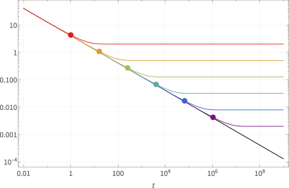
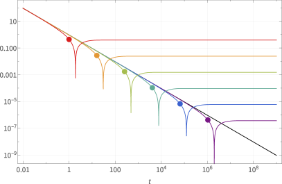
Figure 3: The top frame shows $\phi(t)$ (using (11)) and the bottom frame shows $|\dot{\psi}-C_{1}(\mathcal{A}_{t}-\rho_{c})|$(using (39)) for $\phi_{0}\rightarrow\infty$ and $\rho=\rho_{c}+2^{a}$ with $a$ varying from $a=-20$ (purple) to $a=0$ (red) in steps of $4$. The black lines represent the exactly critical solutions $\rho=\rho_{c}$. The dots placed on each curve signify the handover timescale $t_{\text{ho}}$, which clearly describes well in an order of magnitude manner until what timescale the solutions are well approximated by the critical solutions (20) and (21).

References

- (1) S. A. Hartnoll, C. P. Herzog and G. T. Horowitz, Building a Holographic Superconductor, Phys. Rev. Lett. 101 (2008) 031601 [arXiv:0803.3295].
- (2) S. A. Hartnoll, C. P. Herzog and G. T. Horowitz, Holographic Superconductors, JHEP 12 (2008) 015 [arXiv:0810.1563].
- (3) C. P. Herzog, P. K. Kovtun and D. T. Son, Holographic model of superfluidity, Phys. Rev. D 79 (2009) 066002 [arXiv:0809.4870].
- (4) C. P. Herzog, Lectures on Holographic Superfluidity and Superconductivity, J. Phys. A 42 (2009) 343001 [arXiv:0904.1975].
- (5) S. S. Gubser, Breaking an Abelian gauge symmetry near a black hole horizon, Phys. Rev. D 78 (2008) 065034 [arXiv:0801.2977].
- (6) O. Domenech, M. Montull, A. Pomarol, A. Salvio and P. J. Silva, Emergent Gauge Fields in Holographic Superconductors, JHEP 08 (2010) 033 [arXiv:1005.1776].
- (7) K. Maeda, M. Natsuume and T. Okamura, On two pieces of folklore in the AdS/CFT duality, Phys. Rev. D 82 (2010) 046002 [arXiv:1005.2431].
- (8) P. C. Hohenberg and B. I. Halperin, Theory of dynamic critical phenomena, Rev. Mod. Phys. 49 (Jul, 1977) 435–479.
- (9) K. Maeda, M. Natsuume and T. Okamura, Dynamic critical phenomena in the AdS/CFT duality, Phys. Rev. D 78 (2008) 106007 [arXiv:0809.4074].
- (10) K. Maeda, M. Natsuume and T. Okamura, Universality class of holographic superconductors, Phys. Rev. D 79 (2009) 126004 [arXiv:0904.1914].
- (11) M. Natsuume, Critical phenomena in the AdS/CFT duality, Prog. Theor. Phys. Suppl. 186 (2010) 491–497 [arXiv:1006.4930].
- (12) C. Ewerz, T. Gasenzer, M. Karl and A. Samberg, Non-Thermal Fixed Point in a Holographic Superfluid, JHEP 05 (2015) 070 [arXiv:1410.3472].
- (13) Z. Cai, C. Hubig and U. Schollwöck, Universal long-time behavior of aperiodically driven interacting quantum systems, Phys. Rev. B 96 (Aug, 2017) 054303.
- (14) C. De Grandi, V. Gritsev and A. Polkovnikov, Quench dynamics near a quantum critical point, Phys. Rev. B 81 (Jan, 2010) 012303.
- (15) S. S. Gubser and S. S. Pufu, The Gravity dual of a p-wave superconductor, JHEP 11 (2008) 033 [arXiv:0805.2960].
- (16) P. M. Chesler, A. M. Garcia-Garcia and H. Liu, Defect Formation beyond Kibble-Zurek Mechanism and Holography, Phys. Rev. X 5 (2015), no. 2 021015 [arXiv:1407.1862].
- (17) J. Sonner, A. del Campo and W. H. Zurek, Universal far-from-equilibrium Dynamics of a Holographic Superconductor, Nature Commun. 6 (2015) 7406 [arXiv:1406.2329].
- (18) M. J. Bhaseen, J. P. Gauntlett, B. D. Simons, J. Sonner and T. Wiseman, Holographic Superfluids and the Dynamics of Symmetry Breaking, Phys. Rev. Lett. 110 (2013), no. 1 015301 [arXiv:1207.4194].
- (19) A. del Campo, F. J. Gómez-Ruiz, Z.-H. Li, C.-Y. Xia, H.-B. Zeng and H.-Q. Zhang, Universal statistics of vortices in a newborn holographic superconductor: beyond the Kibble-Zurek mechanism, JHEP 06 (2021) 061 [arXiv:2101.02171].
- (20) Z.-H. Li, H.-Q. Shi and H.-Q. Zhang, Holographic topological defects in a ring: role of diverse boundary conditions, JHEP 05 (2022) 056 [arXiv:2111.15230].
- (21) M. Ammon, S. Grieninger, A. Jimenez-Alba, R. P. Macedo and L. Melgar, Holographic quenches and anomalous transport, JHEP 09 (2016) 131 [arXiv:1607.06817].
- (22) D. Arean, M. Baggioli, S. Grieninger and K. Landsteiner, A holographic superfluid symphony, JHEP 11 (2021) 206 [arXiv:2107.08802].
- (23) D. Sornette, Discrete-scale invariance and complex dimensions, Physics Reports 297 (1998), no. 5 239–270.
- (24) J. Erdmenger, M. Flory, M.-N. Newrzella, M. Strydom and J. M. S. Wu, Quantum Quenches in a Holographic Kondo Model, JHEP 04 (2017) 045 [arXiv:1612.06860].
- (25) E. W. Hirschmann and D. M. Eardley, Universal scaling and echoing in the gravitational collapse of a complex scalar field, Phys. Rev. D 51 (Apr, 1995) 4198–4207.
- (26) I. S. Aranson and L. Kramer, The world of the complex ginzburg-landau equation, Rev. Mod. Phys. 74 (Feb, 2002) 99–143.
- (27) T. Tsuneto, Superconductivity and Superfluidity. Cambridge University Press, 1998.
- (28) P. Wittmer, C.-M. Schmied, T. Gasenzer and C. Ewerz, Vortex motion quantifies strong dissipation in a holographic superfluid, Phys. Rev. Lett. 127 (Aug, 2021) 101601.
- (29) Y.-K. Yan, S. Lan, Y. Tian, P. Yang, S. Yao and H. Zhang, Towards an effective description of holographic vortex dynamics, arXiv:2207.02814.
- (30) P. S. Hagan, Spiral waves in reaction-diffusion equations, SIAM Journal on Applied Mathematics 42 (1982), no. 4 762–786.
- (31) K. Mitman et. al., Nonlinearities in black hole ringdowns, arXiv:2208.07380.
- (32) M. H.-Y. Cheung et. al., Nonlinear effects in black hole ringdown, arXiv:2208.07374.
- (33) A. Adams, P. M. Chesler and H. Liu, Holographic Vortex Liquids and Superfluid Turbulence, Science 341 (2013) 368–372 [arXiv:1212.0281].
- (34) P. M. Chesler and L. G. Yaffe, Numerical solution of gravitational dynamics in asymptotically anti-de Sitter spacetimes, JHEP 07 (2014) 086 [arXiv:1309.1439].
- (35) J. P. Boyd, Chebyshev and Fourier Spectral Methods. Dover Publications Inc., 2003.
- (36) J. Hennig and M. Ansorg, A Fully Pseudospectral Scheme for Solving Singular Hyperbolic Equations on Conformally Compactified Space-Times, J. Hyperbol. Diff. Equat. 6 (2009), no. 01 161–184 [arXiv:0801.1455].
- (37) J. Hennig, Fully pseudospectral time evolution and its application to 1+1 dimensional physical problems, J. Comput. Phys. 235 (2013) 322–333 [arXiv:1204.4220].
- (38) J. Pétri, A spectral method in space and time to solve the advection-diffusion and wave equations in a bounded domain, arXiv:1401.1373.
- (39) R. Panosso Macedo and M. Ansorg, Axisymmetric fully spectral code for hyperbolic equations, J. Comput. Phys. 276 (2014) 357–379 [arXiv:1402.7343].
- (40) J. Hennig and R. Panosso Macedo, Fully pseudospectral solution of the conformally invariant wave equation on a Kerr background, Class. Quant. Grav. 38 (2021), no. 13 135006 [arXiv:2012.02240].
- (41) S. Grieninger, Holographic quenches and anomalous transport, arXiv:1711.08422.
- (42) M. Ammon, D. Arean, M. Baggioli, S. Gray and S. Grieninger, Pseudo-spontaneous symmetry breaking in hydrodynamics and holography, JHEP 03 (2022) 015 [arXiv:2111.10305].
- (43) J. Fernández-Pendás and K. Landsteiner, Out of equilibrium chiral magnetic effect and momentum relaxation in holography, Phys. Rev. D 100 (2019), no. 12 126024 [arXiv:1907.09962].
- (44) I. Amado, D. Arean, A. Jimenez-Alba, K. Landsteiner, L. Melgar and I. S. Landea, Holographic Type II Goldstone bosons, JHEP 07 (2013) 108 [arXiv:1302.5641].
- (45) A. Donos and C. Pantelidou, Higgs/amplitude mode dynamics from holography, JHEP 08 (2022) 246 [arXiv:2205.06294].