Learning a Single Near-hover Position Controller
for Vastly Different Quadcopters

Abstract

This paper proposes an adaptive near-hover position controller for quadcopters, which can be deployed to quadcopters of very different mass, size and motor constants, and also shows rapid adaptation to unknown disturbances during runtime. The core algorithmic idea is to learn a single policy that can adapt online at test time not only to the disturbances applied to the drone, but also to the robot dynamics and hardware in the same framework. We achieve this by training a neural network to estimate a latent representation of the robot and environment parameters, which is used to condition the behaviour of the controller, also represented as a neural network. We train both networks exclusively in simulation with the goal of flying the quadcopters to goal positions and avoiding crashes to the ground. We directly deploy the same controller trained in the simulation without any modifications on two quadcopters in the real world with differences in mass, size, motors, and propellers with mass differing by 4.5 times. In addition, we show rapid adaptation to sudden and large disturbances up to one-third of the mass of the quadcopters. We perform an extensive evaluation in both simulation and the physical world, where we outperform a state-of-the-art learning-based adaptive controller and a traditional PID controller specifically tuned to each platform individually. Video results can be found at https://youtu.be/U-c-LbTfvoA.

I Introduction

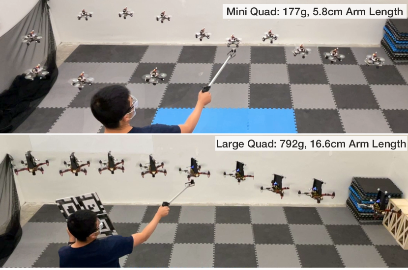
Figure 1: Demonstration of our adaptive controller on two quadrotors with widely varying mass, arm length, and motor constants for the task of tracking a straight and circular trajectory. In the middle of the trajectory, we add a payload unknown to the drone of approximately 30% of the robot’s mass. Our end-to-end controller is able to quickly estimate and react to the disturbance. We use a single control policy across different drones and tasks, which is deployed without any vehicle-specific modifications.

A classic model-based controller for quadcopters requires explicit estimates of the vehicle’s model, including inertia properties (mass and mass moment of inertia), motor constants, and other parameters. Errors in estimating such parameters directly translate to errors in the execution of the controller commands. In addition, once the parameters are estimated, the controller typically requires specific tuning in-flight to achieve the desired behaviour. A modification to the vehicle, e.g., replacing the motors with ones that have different properties, would require repeating the above steps in estimation and tuning. Such significant engineering efforts could be eased with a single controller without specialized tuning. However, this problem raises several challenges since quadcopters are unstable systems. Large variations in quadcopter design have prompted the design of specialized controllers for different quadcopters, as opposed to one single controller. Rejection to disturbances or model uncertainties requires non-trivial design changes to the specialized controllers, which add more layers of complexity to the design work.

In this work, we show a single near-hover position controller aiming to control a variety of quadcopters differing in mass, size, motor, propeller, etc. with mass and planar area size notably differing by at least 10 times. In addition, our controller can rapidly adapt to unknown in-flight disturbances in the mass and inertia changes of the quadcopters. Our work builds on three main insights. The first is that relevant dynamics parameters are observable from the history of states and actions. This has long been known in the community: several works have shown how to estimate parameters online with nonlinear Kalman filters [1, 2] or with neural networks [3]. The second insight is that, at test time, we do not need an estimate of the parameters in some “ground truth” sense. What matters is that the estimate leads to the “right” action, which our end-to-end training procedure optimizes for. This simplifies the estimation problem and avoids observability issues, e.g., identical effects on unobservable or unmatched uncertainties [4]. The third and final insight is that a system can adapt to previously unseen disturbances as long as their effect on the platform dynamics is in the convex hull of the training disturbances (e.g., a motor losing efficiency has a similar effect to adding a payload below the motor).

To realize this, we follow an approach initially proposed for legged robots [5]. However, while that work performs online adaptation to terrains, we use their approach to adapt to a diverse set of quadcopters and perturbations. Specifically, we estimate a latent representation of the quadcopter’s body from a history of sensor observations and actions, which conditions the behaviour of the controller. The diversity of training parameters (Table I) enables adaptation to sudden changes in environment conditions, e.g., a swing payload, for which it was not explicitly trained. Our approach frees drone designers from the estimation and tuning process required any time something changes, or the risk that parameter changes unwittingly cause the control behaviour to significantly change, potentially endangering the system. Furthermore, it naturally lends itself for use in off-the-shelf autopilot systems, allowing users who might otherwise lack the modelling abilities to control a custom vehicle, simply by plugging in the autopilot.

Figure 2: The training (top) and the deployment architecture of our system (bottom). We train in two phases. In the first phase, we train a base policy $\pi$ which takes the current state $x_{t}$, and the intrinsics vector $z_{t}$ which is a compressed version of the environment parameters $e_{t}$ generated by the module $\mu$. Since we cannot deploy this policy in the real world because we do not observe the environment parameters $e_{t}$, we learn an adaptation module which takes the sensor history and action history, and directly predicts the intrinsics vector $z_{t}$. This is done in phase two in simulation using supervised learning. We can finally deploy the base policy $\pi$ which takes as input the current state $x_{t}$ and the intrinsics vector $\hat{z_{t}}$ predicted by the adaptation module $\phi$.

Our approach is related to existing methods in adaptive control. However, our work shifts the meaning of adaptation to a different paradigm. While adaptive control is generally concerned with estimating and counteracting disparities between observations and a reference model, our approach does not have this notion. This key difference enables adaptation to a much wider range of dynamics and disturbances. In addition, it waives the engineering and tuning required by prior work when modifying the vehicle. The closest related to our work are flight controllers in industrial systems like Beta-Flight [6] and PX4 [7]. While they work well across a variety of vehicles, they still require significant in-flight tuning for each robot type and are generally tailored to human pilots.

II Related Work

II-A Traditional Adaptive Control

The design of high-performance adaptive controllers for aerospace systems has been a top priority for researchers and industry for more than 50 years. One of the initial contributions in this space is the model reference adaptive controller (MRAC), an extension of the well-known MIT-rule [8]. The empirical success of this method sparked great interest in the aerospace community, which led to the development of both practical tools and theoretical foundations [9, 10]. From the many methods developed, one of the most popular is $\mathcal{L}_{1}$ adaptive control [11, 4]. The main reason behind its success is the ability to provide rapid adaptation to model uncertainties and disturbances with theoretical guarantees under (possibly restrictive) assumptions. Its high-level working principle consists of estimating the differences between the nominal (as predicted by the reference model) and observed state transitions. Such differences are then compensated by allocating a control authority proportional to the disturbance, effectively driving the system to its reference behaviour. Applications of $\mathcal{L}_{1}$ adaptive controllers for aerial vehicles span from multi-rotors to fixed wings [12, 13].

Mostly related to this work is the application of $\mathcal{L}_{1}$ adaptive control to quadcopters [14]. However, the performance of the classic $\mathcal{L}_{1}$ formulation degrades whenever the observed transitions differ greatly from the (usually linear) reference model, which can happen due to aerodynamic effects or large payloads. Therefore, recent work has combined $\mathcal{L}_{1}$ adaptive control with nonlinear online optimization [15, 16, 17]. While these methods achieved impressive results, they still require explicit knowledge of (reference) system parameters, such as inertia, mass, and motor characteristics. In addition, they generally require platform-specific tuning to get the desired behaviour. Other approaches to adaptive control on quadcopters include differential flatness [18] and nonlinear dynamic inversion [19]. These methods have shown rapid adaptation to aerodynamic effects and model uncertainties. However, they cannot cope with large variations in the quadcopter’s dynamics, since the underlying assumptions on locally linear disturbances are generally not fulfilled.

II-B Learning-Based Adaptive Control

Recent data-driven controllers have shown promising results for quadcopter stabilization [20, 21], or waypoint tracking flight [22, 23]. As their classic counterparts, learning-based controllers also allow for adaptation to disturbances and model mismatches. One possibility to do so consists of learning a model from the data and using the model to adapt the controller [24, 25, 26, 27]. However, this has the limitation that the models are difficult to carefully identify due to under-actuation of the platform and sensing noise. This motivated model-free methods that, like ours, learn an end-to-end adaptive policy [28]. Meta-learning has also been proposed to augment the performance of the model-based controller for fast online adaptation to wind [29] or suspended payloads [26]. These methods achieved impressive results in disturbance rejection. However, they are still tailored to a specific platform type, and lack an explicit mechanism for adaptation to drastic changes in the drone’s model and actuation. They also require relatively expensive real world learning samples. Our work aims to fill this gap and create a single control policy capable of flying vehicles with vastly varying physical characteristics and under large disturbances.

III Learning an Adaptive Drone Controller

We learn a single position controller to fly quadcopters to target positions and stay hovering. This controller takes a history of platform states and commands from a platform-independent high level controller as inputs, and outputs individual motor speed. Our resulting policy can control quadcopters with very different design and hardware characteristics, and is robust to disturbances unseen at training time, such as swing payloads and malfunctioning motors. To achieve this, we use RMA [5]. However, we re-purpose the adaption module, originally used to estimate parameters external to the robot, e.g. friction, to estimate the robot’s intrinsic parameters (e.g. its mass, inertia, motor constant, etc.). In the following, we recapitulate the method of RMA for completeness. Our policy consists of a base policy $\pi$ and an adaptation module $\phi$. At time $t$, the base policy $\pi$ takes the current state $x_{t}\in\mathbb{R}^{23}$ and an intrinsics vector $z_{t}\in\mathbb{R}^{6}$ as input and outputs the target motor speeds $a_{t}\in\mathbb{R}^{4}$ for all individual motors. The current state $x_{t}$ includes the vehicle’s position, velocity, rotation matrix, mass-normalized thrust, angular velocity, commanded total thrust and commanded angular velocity. The intrinsics vector $z_{t}$ is a low dimensional encoding of the environment parameters $e_{t}$ containing drone parameters, payload, etc. It allows the base policy to adapt to variations in drone parameters, payloads, and disturbances such as external force or torque. Since we cannot directly measure $z_{t}$ in the real world, we instead estimate it via the adaptation module $\phi$, which uses the discrepancy between the commanded actions and the measured sensor readings from the latest $k$ steps to estimate it online during deployment. More concretely,

$$\hat{z_{t}} =\phi\big{(}x_{t-k:t-1},a_{t-k:t-1}\big{)}$$ (1)

$$a_{t} =\pi(x_{t},\hat{z_{t}})$$ (2)

III-A Base Policy

We learn the base policy $\pi$ in simulation using model-free Reinforcement Learning (RL). During training, the base policy takes the current state $x_{t}$ and the ground-truth intrinsics vector $z_{t}$ to output control commands $a_{t}$. We use the environmental factor encoder $\mu$ to compress $e_{t}$ to $z_{t}$. This gives us:

$$z_{t} =\mu(e_{t})$$ (3)

$$a_{t} =\pi(x_{t},z_{t})$$ (4)

We implement $\mu$ and $\pi$ as Multi-layer perceptrons (MLP) and jointly train the base policy $\pi$ and the environmental factor encoder $\mu$ end-to-end using model-free RL. RL maximizes the following expected return of the policy $\pi$:

$$J(\pi)=\mathbb{E}_{\tau\sim p(\tau|\pi)}\Bigg{[}\sum_{t=0}^{T-1}\gamma^{t}r_{t}\Bigg{]},$$ (5)

where $\tau=\{(x_{0},a_{0},r_{0}),(x_{1},a_{1},r_{1})...\}$ is the trajectory of the agent when executing the policy $\pi$, and $p(\tau|\pi)$ represents the likelihood of the trajectory under $\pi$.

RL Reward

The following reward function encourages the agent to hover at a goal position and penalizes crashes and oscillating motions. Let us denote the acceleration in the body-fixed thrust axis, i.e. the mass-normalized thrust as $c$, the angular velocity as $\bm{\omega}$, all in the quadcopter’s body frame. The commanded mass-normalized thrust is defined as $c_{des}$, commanded angular velocity as $\bm{\omega}_{des}$, all given by the high-level controller. We additionally define the motor speeds as $\bm{m}$ and the simulation step in the training as $\delta t$. The reward at time $t$ is defined as the sum of the following quantities:

1. Angular Velocity Tracking Deviation Penalty:
   $-\|\bm{\omega}^{t}-\bm{\omega}_{des}^{t}\|$

2. Mass-normalized Thrust Tracking Deviation Penalty: $-\|{c}^{t}-{c}_{des}^{t}\|$

3. Output Command Oscillation Penalty: $-\|\bm{m}^{t}-\bm{m}^{t-1}\|$

4. Survival Reward: $\delta t$

The scaling factor of each reward term is $0.01$, $0.02$, $0.0002$, $1$ respectively.

TABLE I: Ranges of the drone and environmental parameters. Parameters without units labelled are dimensionless quantities.

Parameters	Training Range	Testing Range
Mass (kg)	[0.142, 0.950]	[0.114, 1.140]
Arm length (m)	[0.046, 0.200]	[0.037, 0.240]
Mass moment of inertia	[7.42e-5 , 5.60e-3]	[5.94e-5 , 6.72e-3]
around $x$, $y$ (kg$\cdot$m2)
Mass moment of inertia	[1.20e-4, 8.80e-3]	[9.60e-5, 1.06e-2]
around $z$ (kg$\cdot$m2)
Propeller constant $\kappa$ (m)	[0.0041, 0.0168]	[0.0033, 0.0201]
Payload (% of Mass)	[10, 50]	[5, 60]
Payload Location	[-10, 10]	[-10, 10]
from Center of Mass
(% of Arm length)
Motor Constant	[1.15e-7, 7.64e-6]	[9.16e-8, 9.17e-6]
Body drag coefficient	[0, 0.62]	[0, 0.74]
Max. motor speed (rad/s)	[707, 4895]	[566, 5874]

III-B Adaptation Module

During deployment, we do not have access to the vector $e_{t}$ and hence we cannot compute the intrinsics vector $z_{t}$. Instead, we will use the sensor and action history to directly estimate $z_{t}$ as proposed in [5]. We call this module the adaptation module $\phi$. We can train this module in simulation using supervised learning because we have access to both the ground truth intrinsics $z_{t}$, and the sensor history and previous actions. We minimize the mean squared error loss $\lVert z-\hat{z}\rVert^{2}$.

III-C Deployment

We directly deploy the base policy $\pi$ which uses the current state $x_{t}$ and the intrinsics vector $\hat{z_{t}}$ predicted by the adaptation module $\phi$. We do not calibrate or finetune our policy, and use the same policy without any modifications on the different drones under different payload and conditions.

IV Experimental Setup

Simulation Environment. We use the Flightmare simulator [30] for training and testing our control policies. We implement the same high-level controller in [31] to generates high-level commands at the level of body rates and collective thrust. It is designed as a cascaded linear acceleration controller with desired acceleration mimicking a spring-mass-damper system with natural frequency 2rad/s and damping ratio 0.7. The desired acceleration is then converted to a desired total thrust and the desired thrust direction, and the body rates are computed from this as proportional to the attitude error angle, with a time constant of 0.2s. We define the task as hovering at a pre-defined location. This high-level controller’s inputs are the platform’s state (position, rotation, angular, and linear velocities) and the goal location. The policy outputs individual motor speed commands, and we model the motors’ response using a first-order system. Each RL episode lasts for a maximum of 5s of simulated time, with early termination if the quadcopter height drops below 2cm. The control frequency of the policy is $500$Hz, and the simulation step is 2ms. We additionally implement an observation latency of 10ms.

Quadcopter and Environment Randomization. All our training and testing ranges in simulation are listed in Table I. Of these, $e_{t}$ includes mass, arm length, propeller torque to thrust ratio $\kappa$, motor constant, inertia ($\mathbb{R}^{3\times 3}$), body drag coefficients ($\mathbb{R}^{3}$), maximum motor rotation and payload mass, which results in an 18 dimensional vector. We randomize each of these parameters at the end of each episode. In addition, at a randomly sampled time during each episode, the parameters including mass, inertia, and the center of mass are also randomized. The latter is used to mimic sudden variations in the quadcopter parameters due to a sudden disturbance caused by a payload or wind.

Hardware Details. For all our real-world experiments we use two quadcopters, which differ in mass by a factor of 4.5, and in arm length by a factor of 2.9. The first one, which we name largequad has a mass of 792g, a size of 16.6cm in arm length, a thrust-to-weight ratio of 3.50, a diagonal inertia matrix of [0.0047, 0.005, 0.0074]kg$\cdot$m² (as expressed in the z-up body-fixed frame), and a maximum motor speed of 943rad/s. The second one, miniquad, has a mass of 177g, a size of 5.8cm in arm length, a thrust-to-weight ratio of 3.45, a diagonal inertia matrix of [92.7e-6, 92.7e-6, 158.57e-6]kg$\cdot$m², and a maximum motor speed of 3916rad/s. A motion capture system running at $200$Hz provides estimates of the drone position and orientation, which is followed by a Kalman filter to reduce noise and estimate linear velocity. An onboard rate gyroscope measures the angular rotation of the robot, which is low-pass filtered to reduce noise and remove outliers. The deployed policy outputs motor speed commands, which are subsequently tracked by off-the-shelf electronic speed controllers. We use as high-level a PD controller which takes as input the goal position and outputs the mass normalized collective trust and the body rates.

Network Architecture and Training Procedure. The base policy is a 3-layer MLP with 256-dim hidden layers. This takes the drone state and the vector of intrinsics as input to produce motor speeds. The environment factor encoder is a 2-layer MLP with 128-dim hidden layers. The policy and the value function share the same factor encoding layer. The adaptation module projects the latest 400 state-action pairs into a 128-dim representation, with the state-action history initialized with zeros. Then, a 3-layer 1-D CNN convolves the representation across time to capture its temporal correlation. The input channel number, output channel number, kernel size and stride of each CNN layer are [32, 32, 8, 4], [32, 32, 5, 1], [32, 32, 5, 1]. The flattened CNN output is linearly projected to estimate $z_{t}$. We train the base policy and the environment encoder using PPO [32] for 100M steps. We use the reward outlined in Section III. Policy training takes approximately 2 hours on an ordinary desktop machine with 1 GPU. We finally train the adaptation module with supervised learning by rolling out the student policy. We train with the ADAM optimizer to minimize MSE loss. We run the optimization process for 10M steps, training on data collected over the last 1M steps. Training the adaptation module takes approximately 20 minutes.

V Results

Figure 3: Upper Left: Large and small quadcopters mounted with an inertia board. For the large quadcopter, we mount a wrench of 20.5cm and 140g. For the small quadcopter, a wrench of 14.5cm and 30g. Upper Right: Large and small quadcopters with a rigid payload. For the former, we add a load of 180g ($\approx 25\%$ of its weight). For the latter, we add a load of 50g, which corresponds to 35.7% of its weight. Lower Left: Large and small quadcopters with random pushes/pulls. Lower Right: Large and small quadcopters with a swing payload, which is the wrench in the inertia board test. Despite such large disturbances unknown to the control policy, our approach can always stabilize the quadcopter.

TABLE II: Real-World Results: We compare the performance of our controller to two baselines: LTF and a PID controller. The comparison is run on three tasks for large and small quadcopters. Free Hover: hover at the goal position without any disturbances. Inertia Board: hover at the goal position under an unknown mass and inertia disturbance. Payload: hover at the goal position under an unknown mass disturbance. Metrics are averaged over 5 experiments.

	Vehicle	Method	Height	Ang. Vel.	Thrust	Success
			Err. (m)	Err. (rad/s)	Err. (m/s2)	Rate
Free Hover	small	PID	0.06	0.51	0.57	100
		LTF [33]	0.09	0.78	0.78	80
		Ours	0.05	0.30	0.30	100
	large	PID	0.01	0.12	0.28	100
		LTF [33]	0.03	1.21	1.86	80
		Ours	0.03	0.19	0.36	100
Inertial Board	small	PID	-	-	-	0
		LTF [33]	-	-	-	0
		Ours	0.08	1.14	1.09	100
	large	PID	0.31	0.37	1.46	100
		LTF [33]	-	-	-	0
		Ours	0.08	0.24	1.35	100
Payload	small	PID	0.40	1.14	2.20	80
		LTF [33]	0.10	0.98	2.14	100
		Ours	0.05	0.88	0.51	100
	large	PID	0.19	1.14	1.21	100
		LTF [33]	0.06	1.01	4.2	100
		Ours	0.04	0.34	1.19	100

V-A Real World Deployment

We test our approach in the physical world and compare its performance to two baselines: LTF, which is a learning-based robust controller trained with an error integration as one of inputs, aiming to control hybrid UAVs [33]; and a platform-specific PID controller. The PID controller has access to the platform’s mass and inertia, and it has been specifically tuned to the platform with in-flight tests. In contrast, our approach has no knowledge whatsoever of the physical characteristics of the system and requires no calibration or real-world fine tuning. We compare the task of stabilization to a predefined set point without any disturbances (free hover), or under an unknown mass and/or inertia disturbance (Figure 3).

We compare the three approaches under four metrics: (i) the average height error to the goal point, and the average tracking error of the (ii) angular velocity and (iii) mass normalized thrust of the high-level controller’s commands, and the success rate. We define a failure if the human operator had to intervene to avoid the quadcopter from crashing. The results of these experiments are reported in table II.

Our approach significantly outperforms both baselines in all metrics under all disturbances. In particular, our approach achieves a 100% success rate when asymmetric disturbances are applied to the system, while the two baselines both experience at least one total failure on either of the two platforms. The PID baseline and our approach performs similarly in free hovering experiment, with the PID controller slightly outperforming ours on largequad. The latter difference in performance is justified, since the PID controller is specifically tuned for each quadcopter, but ours does not have knowledge of the system dynamics and hardware.

V-B Simulation Results

TABLE III: Simulation Testing Results: We compare our method with four baselines on the task of stabilization: Robust, SysID, LTF, and $\mathcal{L}_{1}$. We also list the results of our method in Phase I training, which has access to all ground-truth system parameters and can be regarded as the expert. The test ranges are defined in Table I. Metrics are averages over 100 experiments.

	Success	Height	Ang. Vel.	Thrust
	Rate	Err. (m)	Err. (rad/s)	Err. (m/s2)
Robust [34, 35]	18%	0.44	1.32	1.93
SysID [36]	38%	0.19	1.10	1.38
LTF [33]	59%	0.35	0.97	1.68
$\mathcal{L}_{1}$ [15]	59%	0.17	0.92	1.60
Ours	66%	0.09	0.94	1.57
Expert (Phase I)	69%	0.09	0.91	1.29

TABLE IV: Simulation Testing Results, Out-of-Distribution Disturbances: We evaluate the performance of our method and all baselines on two types of disturbances unseen at training time. External Forces: We apply a random force of magnitude uniformly sampled between 0 and 50% of the weight and with direction uniformly sampled on a cube. Partially Failing Motors: To simulate a motor losing efficiency, we multiply the output of a randomly sampled motor’s thrust force to a random number between 0 and 1. The duration of each disturbance is random between the entire length of the episode (on and off with 2% probability at every time stamp).

External Forces	Success	Height	Ang. Vel.	Thrust
	Rate	Err. (m)	Err. (rad/s)	Err. (m/s2)
Robust [34, 35]	5%	0.39	2.05	1.51
SysID [36]	2%	0.22	1.38	1.23
LTF [33]	32%	0.23	1.53	0.99
$\mathcal{L}_{1}$ [15]	42%	0.30	1.46	1.04
Ours	49%	0.09	1.40	0.85
Partially Failing Motors
Robust [34, 35]	1%	0.53	1.94	1.59
SysID [36]	14%	0.33	1.25	1.23
LTF [33]	21%	0.38	1.57	1.35
$\mathcal{L}_{1}$ [15]	33%	0.32	1.41	1.06
Ours	38%	0.26	1.36	1.01

Finally, we compare our approach with a set of baselines in the simulation. We select four baselines from prior work: Robust, which consists of a policy trained without access to environment factors or body parameters [35, 34]; SysID, which directly predicts the ground-truth parameters $e_{t}$ [36] instead of the low-dimensional intrinsics vector; LTF, which essentially is a robust policy with an error integration as additional inputs [33]; and $\mathcal{L}_{1}$, a model-based adaptive controller which estimates and compensates the difference between the nominal and observed states to achieve adaptive control [11, 4, 15]. We keep the same architecture and hyperparameters as ours for all learning-based baselines. Similarly to real-world experiments, we evaluate on the task of stabilization. The testing ranges are listed in Table I. We rank the methods according to the success rate, the average height error, and the tracking performance. At the beginning of each experiment, the quadcopter is spawned with a random orientation, a random position in x-y of [-1,1] and [0.5, 2.5] in z, and a random velocity on each axis of [-1,1]. The experiment is considered successful if the end height of the quadcopter is within 0.3m from the goal height. The results of these experiments are reported in Table III.

Given the very large amount of quadcopter variations, the Robust baseline trained without access to environment parameters has the lowest success rate and largest tracking error. This is because it is forced to learn a single conservative controller which can fly all quadcopters under varying disturbances. Indeed, it either crashes to the ground or flies outside the flying region. The baseline LTF is Robust with an additional observation of error integration. This additional input helps it achieve higher success rate. However, similar to the Robust baseline, LTF fails in tracking the goal states. On the contrary, with estimation of the environment parameters, the flight performance strongly increases.

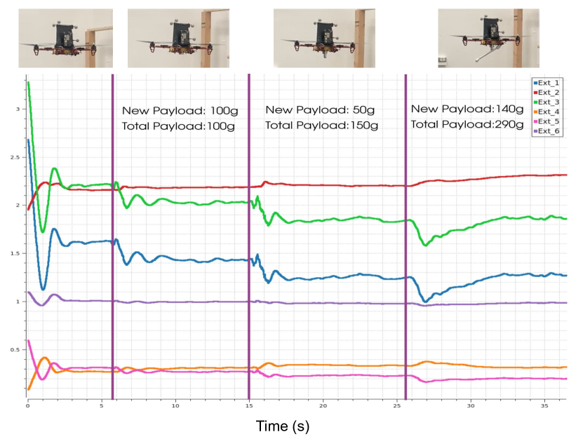
Figure 4: We analyze the change in behaviour of our policy as we incrementally add total 290g payloads to our largequad. We plot all 6 components of the intrinsics vector $\hat{z_{t}}$ predicted by the adaptation module. We see that changes in intrinsics are strongly correlated with disturbances applied to the quadcopter, indicating that the added payloads have been detected by the adaptation module. When the payload is added, the quadcopter first sinks and then recovers to the normal motion. The plotted components of the intrinsics vector change in response to the disturbance, from which we know the adaptation period takes around 2s.

Still, explicitly regressing the environment vector $e_{t}$, instead of its low-dimensional representation $z_{t}$, yields the success rate since it is trying to solve a harder estimation problem which is not necessary to solve the task at hand. Since the tracking errors are computed only for successful runs, the SysID baseline achieves a slightly lower tracking error in one of the metrics. $\mathcal{L}_{1}$ is the baseline with the strongest performance in our simulation experiments. However, its strong performance relies on the explicit knowledge of a reference model which we choose as the median value of all parameters in the testing range in Table I, while our method with other baselines has no prior knowledge of the model. The performance gap between our method and $\mathcal{L}_{1}$ shows that the adaptive control across platforms is hard to achieve by estimating and compensating large variance from a reference model. $\mathcal{L}_{1}$ is not implemented in our real-world experiments as a baseline because it is highly sensitive to latency and requires significant engineering work. In contrast, our approach can handle latency very well by simulating it during training.

We also evaluate the task of stabilization on held-out environmental disturbances, as exemplified by random external forces and partial failure of a motor. The results of these experiments are reported in Table IV. Our method outperforms all baselines in both out-of-distribution disturbances cases. Compared to the strongest baseline $\mathcal{L}_{1}$, our method has a greater success rate, and it reduces the average height error by up to 67.7% and the average command tracking error by up to 22.4%.

V-C Adaptation Analysis

We analyze the estimated intrinsics vector $\hat{z_{t}}$ for adaptation on incremental payloads. We incrementally add payloads in total of 290g to the largequad in hovering. The quadcopter adapts successfully to payloads and stabilizes itself at the target position. We plot all components of the estimated intrinsics vector from the adaptation module during the experiment in Figure 4. We find that whenever a payload is applied, there is a change in all intrinsics components. From the change of the plotted components of intrinsics vector in response to the disturbance, we see that it takes around 2s for our controller to detect the disturbance, estimate the intrinsics vector, adapt to the disturbance, and remain hovering at the target location. The adaptation period of our controller is much faster than that of methods with online estimation of ground truth model parameters such as [2], where it takes 10s to 15s in-flight to obtain an accurate model estimate.

VI Conclusion

In this work, we show how a single policy can control quadcopters of totally different size, mass, and actuation. We successfully transfer a method initially developed for legged locomotion in adapting terrains to quadcopters in adapting a diverse set of quadcopter bodies and disturbances. Without any additional tuning or modification, the single policy trained only in simulation can be deployed zero-shot to quadcopters of very different design and hardware characteristics while showing rapid adaptation to unknown disturbances at the same time. However, our current controller is a quasi-static position controller which fails on tracking aggressive flights. Future work should focus on improving its ability to track arbitrary trajectories to achieve a universal quadcopter controller.

VII Acknowledgement

This work was supported by the DARPA Machine Common Sense program, Hong Kong Center for Logistics Robotics, and the Graduate Division Block Grant of the Dept. of Mechanical Engineering, UC Berkeley. The experimental testbed at the HiPeRLab is the result of contributions of many people, a full list of which can be found at hiperlab.berkeley.edu/members/. This work was also partially supported by the ONR MURI award N00014-21-1-2801.

References

- [1] J. Svacha, J. Paulos, G. Loianno, and V. Kumar, “Imu-based inertia estimation for a quadrotor using newton-euler dynamics,” IEEE Robotics and Automation Letters, vol. 5, no. 3, pp. 3861–3867, 2020.
- [2] V. Wüest, V. Kumar, and G. Loianno, “Online estimation of geometric and inertia parameters for multirotor aerial vehicles,” in 2019 International Conference on Robotics and Automation (ICRA). IEEE, 2019, pp. 1884–1890.
- [3] M. Forgione and D. Piga, “Continuous-time system identification with neural networks: Model structures and fitting criteria,” European Journal of Control, vol. 59, pp. 69–81, 2021.
- [4] N. Hovakimyan and C. Cao, L1 adaptive control theory: Guaranteed robustness with fast adaptation. SIAM, 2010.
- [5] A. Kumar, Z. Fu, D. Pathak, and J. Malik, “Rma: Rapid motor adaptation for legged robots,” RSS: Robotics Science and Systems, 2021.
- [6] “Betaflight: Open source flight controller firmware,” https://betaflight.com/.
- [7] “Open source autopilot for drones: Px4 autopilot,” https://px4.io/.
- [8] I. M. Mareels, B. D. Anderson, R. R. Bitmead, M. Bodson, and S. S. Sastry, “Revisiting the mit rule for adaptive control,” IFAC Proceedings Volumes, vol. 20, no. 2, pp. 161–166, 1987.
- [9] K. J. Åström and B. Wittenmark, Adaptive control. Courier Corporation, 2013.
- [10] E. Lavretsky and K. A. Wise, “Robust adaptive control,” in Robust and adaptive control. Springer, 2013, pp. 317–353.
- [11] C. Cao and N. Hovakimyan, “Design and analysis of a novel l1 adaptive control architecture with guaranteed transient performance,” IEEE Transactions on Automatic Control, vol. 53, no. 2, pp. 586–591, 2008.
- [12] S. Mallikarjunan, B. Nesbitt, E. Kharisov, E. Xargay, N. Hovakimyan, and C. Cao, “L1 adaptive controller for attitude control of multirotors,” in AIAA guidance, navigation, and control conference, 2012, p. 4831.
- [13] I. Gregory, C. Cao, E. Xargay, N. Hovakimyan, and X. Zou, “L1 adaptive control design for nasa airstar flight test vehicle,” in AIAA guidance, navigation, and control conference, 2009, p. 5738.
- [14] M. Schreier, “Modeling and adaptive control of a quadrotor,” in 2012 IEEE international conference on mechatronics and automation. IEEE, 2012, pp. 383–390.
- [15] D. Hanover, P. Foehn, S. Sun, E. Kaufmann, and D. Scaramuzza, “Performance, precision, and payloads: Adaptive nonlinear mpc for quadrotors,” IEEE Robotics and Automation Letters, vol. 7, no. 2, pp. 690–697, 2021.
- [16] J. Pravitra, K. A. Ackerman, C. Cao, N. Hovakimyan, and E. A. Theodorou, “L1-adaptive mppi architecture for robust and agile control of multirotors,” in 2020 IEEE/RSJ International Conference on Intelligent Robots and Systems (IROS). IEEE, 2020, pp. 7661–7666.
- [17] K. Pereida and A. P. Schoellig, “Adaptive model predictive control for high-accuracy trajectory tracking in changing conditions,” in 2018 IEEE/RSJ International Conference on Intelligent Robots and Systems (IROS). IEEE, 2018, pp. 7831–7837.
- [18] M. Faessler, A. Franchi, and D. Scaramuzza, “Differential flatness of quadrotor dynamics subject to rotor drag for accurate tracking of high-speed trajectories,” IEEE Robotics and Automation Letters, vol. 3, no. 2, pp. 620–626, 2017.
- [19] E. J. Smeur, Q. Chu, and G. C. De Croon, “Adaptive incremental nonlinear dynamic inversion for attitude control of micro air vehicles,” Journal of Guidance, Control, and Dynamics, vol. 39, no. 3, pp. 450–461, 2016.
- [20] J. Hwangbo, I. Sa, R. Siegwart, and M. Hutter, “Control of a quadrotor with reinforcement learning,” IEEE Robotics and Automation Letters, vol. 2, no. 4, pp. 2096–2103, 2017.
- [21] W. Koch, R. Mancuso, R. West, and A. Bestavros, “Reinforcement learning for uav attitude control,” ACM Transactions on Cyber-Physical Systems, vol. 3, no. 2, pp. 1–21, 2019.
- [22] Y. Song, M. Steinweg, E. Kaufmann, and D. Scaramuzza, “Autonomous drone racing with deep reinforcement learning,” in 2021 IEEE/RSJ International Conference on Intelligent Robots and Systems (IROS). IEEE, 2021, pp. 1205–1212.
- [23] E. Kaufmann, L. Bauersfeld, and D. Scaramuzza, “A benchmark comparison of learned control policies for agile quadrotor flight,” arXiv preprint arXiv:2202.10796, 2022.
- [24] N. O. Lambert, D. S. Drew, J. Yaconelli, S. Levine, R. Calandra, and K. S. Pister, “Low-level control of a quadrotor with deep model-based reinforcement learning,” IEEE Robotics and Automation Letters, vol. 4, no. 4, pp. 4224–4230, 2019.
- [25] G. Shi, X. Shi, M. O’Connell, R. Yu, K. Azizzadenesheli, A. Anandkumar, Y. Yue, and S.-J. Chung, “Neural lander: Stable drone landing control using learned dynamics,” in 2019 International Conference on Robotics and Automation (ICRA). IEEE, 2019, pp. 9784–9790.
- [26] S. Belkhale, R. Li, G. Kahn, R. McAllister, R. Calandra, and S. Levine, “Model-based meta-reinforcement learning for flight with suspended payloads,” IEEE Robotics and Automation Letters, vol. 6, no. 2, pp. 1471–1478, 2021.
- [27] G. Torrente, E. Kaufmann, P. Föhn, and D. Scaramuzza, “Data-driven mpc for quadrotors,” IEEE Robotics and Automation Letters, vol. 6, no. 2, pp. 3769–3776, 2021.
- [28] C.-H. Pi, W.-Y. Ye, and S. Cheng, “Robust quadrotor control through reinforcement learning with disturbance compensation,” Applied Sciences, vol. 11, no. 7, p. 3257, 2021.
- [29] M. O’Connell, G. Shi, X. Shi, K. Azizzadenesheli, A. Anandkumar, Y. Yue, and S.-J. Chung, “Neural-fly enables rapid learning for agile flight in strong winds,” Science Robotics, vol. 7, no. 66, p. eabm6597, 2022.
- [30] Y. Song, S. Naji, E. Kaufmann, A. Loquercio, and D. Scaramuzza, “Flightmare: A flexible quadrotor simulator,” in Proceedings of the 2020 Conference on Robot Learning, 2021, pp. 1147–1157.
- [31] M. W. Mueller, “Multicopter attitude control for recovery from large disturbances,” arXiv preprint arXiv:1802.09143, 2018.
- [32] J. Schulman, F. Wolski, P. Dhariwal, A. Radford, and O. Klimov, “Proximal policy optimization algorithms,” arXiv preprint arXiv:1707.06347, 2017.
- [33] J. Xu, T. Du, M. Foshey, B. Li, B. Zhu, A. Schulz, and W. Matusik, “Learning to fly: computational controller design for hybrid uavs with reinforcement learning,” ACM Transactions on Graphics (TOG), vol. 38, no. 4, pp. 1–12, 2019.
- [34] X. B. Peng, M. Andrychowicz, W. Zaremba, and P. Abbeel, “Sim-to-real transfer of robotic control with dynamics randomization,” in 2018 IEEE international conference on robotics and automation (ICRA). IEEE, 2018, pp. 3803–3810.
- [35] J. Tobin, R. Fong, A. Ray, J. Schneider, W. Zaremba, and P. Abbeel, “Domain randomization for transferring deep neural networks from simulation to the real world,” in 2017 IEEE/RSJ international conference on intelligent robots and systems (IROS). IEEE, 2017, pp. 23–30.
- [36] W. Yu, J. Tan, C. K. Liu, and G. Turk, “Preparing for the unknown: Learning a universal policy with online system identification,” in Robotics: Science and Systems XIII, Massachusetts Institute of Technology, Cambridge, Massachusetts, USA, July 12-16, 2017, N. M. Amato, S. S. Srinivasa, N. Ayanian, and S. Kuindersma, Eds., 2017. [Online]. Available: http://www.roboticsproceedings.org/rss13/p48.html