Discriminative Sampling of Proposals in Self-Supervised Transformers
for Weakly Supervised Object Localization

Abstract

Drones are employed in a growing number of visual recognition applications. A recent development in cell tower inspection is drone-based asset surveillance, where the autonomous flight of a drone is guided by localizing objects of interest in successive aerial images. In this paper, we propose a method to train deep weakly-supervised object localization (WSOL) models based only on image-class labels to locate object with high confidence. To train our localizer, pseudo labels are efficiently harvested from a self-supervised vision transformers (SSTs). However, since SSTs decompose the scene into multiple maps containing various object parts, and do not rely on any explicit supervisory signal, they cannot distinguish between the object of interest and other objects, as required WSOL. To address this issue, we propose leveraging the multiple maps generated by the different transformer heads to acquire pseudo-labels for training a deep WSOL model. In particular, a new Discriminative Proposals Sampling (DiPS) method is introduced that relies on a CNN classifier to identify discriminative regions. Then, foreground and background pixels are sampled from these regions in order to train a WSOL model for generating activation maps that can accurately localize objects belonging to a specific class. Empirical results on the challenging TelDrone dataset indicate that our proposed approach can outperform state-of-art methods over a wide range of threshold values over produced maps. We also computed results on CUB dataset, showing that our method can be adapted for other tasks.

1 Introduction

Due to its efficiency and flexibility, drone based surveillance has recently emerged as a feasible alternative for monitoring assets at numerous cell tower sites. Globally, millions of cell towers are being monitored for verification of assets, e.g., antennas. However, manual cell tower inspection is highly dangerous and expensive [2]. To deploy drones for surveillance we need to localize objects that help drones to fly autonomously. Additionally, once a drone is able to identify and localize objects, it can perform different visual recognition tasks. For visual recognition, the drone should be able to fly at a safe distance from obstacles. Given the difficulty incurred in acquiring aerial images of concerned object at different viewpoints, and their associated bounding box annotations, we are unable to employ object localization models trained using supervised learning. To deal with this issue, we propose using model that can efficiently learn to localize objects of interest in a weakly-supervised manner [12], and efficiently guide the drone as it captures cell tower.

Commonly used methods for weakly supervised object localization are based on class activation maps (CAMs) built on top of standard convolutional neural networks (CNNs) [7, 14, 25, 33, 37, 46, 47, 54, 55, 56, 58, 60]. These methods allow producing a spatial class activation map highlighting features belonging to a particular class using features from the penultimate layer [62] of a CNN. Strong activation of a map indicates the potential presence of the corresponding class, allowing for object localization. To improve the robustness of CAM methods, several techniques have been proposed to obtain maps from different layers by utilizing gradient information [16, 36, 10]. Despite their popularity, CAM methods have limitations leading to inaccurate localization. Activation maps tend to focus on small discriminant areas of objects [7, 5] – common to different instances of an object belonging to a specific class. Current efforts in the WSOL litterature focus on improving the CAMs to cover the full object. However, for aerial cell tower photos, regions of interest (RoI) are quite small relative to the entire images, and can be quite distant from the drone. Hence, current CAM-based methods produce bloby results, and are unable to adequately localize objects [7, 29].

Recently, self-supervised transformers (SSTs) [9] has attracted much attention for WSOL tasks. Using only self-supervision, these models can yield impressive saliency maps. Given their long-range receptive fields, SSTs analyze an entire input image, allowing them to build saliency maps that cover full objects. Transformers are able to identify multiple objects by decomposing the scene into different spatial saliency maps. Such localization information is accumulated in maps, i.e. class tokens, at the top layer (see Fig. 1(b)). However, without any class supervision, these tokens are arbitrary and class-agnostic, and objects of interest cannot be dissociated from others. Each token focuses on a random object with semantics that differ from one image to another, making them less reliable for localization. Unless ground truth localizations are provided to select the best token [9], their application in WSOL remains limited.

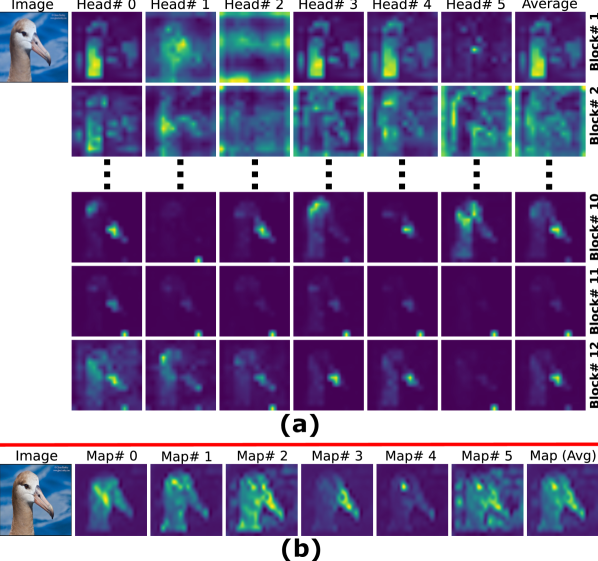
Figure 1: (a): Attention of each class token learned by TS-CAM [17] map from the first two and last three blocks. The first half of the blocks attends to different features, including background regions, but TS-CAM is able to accumulate all of them. Attention maps of each class token are shown in Supplementary Material. (b): The attention map of class tokens corresponding to each token head from the last layer of transformer learned in a self-supervised fashion. These maps show that the last layer is capable of accumulating fine-grained localization of the concerned object.

Few recent work have been proposed to extract discriminative localization from class tokens. In particular, TS-CAM [17] has been proposed to leverage localization in transformers, where the average of all class tokens is multiplied with a semantic-aware map to produce the final activation map. Since TS-CAM averages an abundance of class-agnostic attention maps, it is prone to localization error by including non-discriminative regions. Additionally, maps from earlier layers attend to background regions, as shown in Fig.1(a). Therefore, accumulating all maps introduces noise in the final activation map that can reduce the model’s localization accuracy. Different transformer-based methods have been proposed [3, 11, 19, 39]. [3] propose a spatial calibration module to capture semantic relationships and spatial similarities. Similarly, ViTOL [19] proposes to incorporate a patch-based attention dropout layer into the transformer attention blocks to improve localization maps. [11] proposes a relational patch-attention module to enhance local perception quality, and to retain global information. [39] introduces a mechanism to suppress background regions and focus on the target object. All these methods are unable to minimize the loss over the localization maps as they solely focus on classification tasks, limiting their ability to fully cover an object while requiring a search for an optimal threshold.

In this paper, a new Discriminative Proposals Sampling (DiPS) method is proposed to leverage localization information from SSTs for accurate WSOL in aerial images captured by drones. During training, class token maps are extracted from the top block of pretrained SST. Given a limited number of high-quality attention maps (class tokens) covering different objects, we employ a CNN classifier to localize potential discriminative regions (see Fig. 1(a)). Then, pixel-wise pseudo-labels are sampled from these regions to train a U-Net style localization network. To benefit from these tokens, a method is introduced for collecting appropriate pseudo-labels, and sampling foreground/background regions from them to train our localization network such that a particular object can be localized with a high level of confidence (Fig.2). In particular, with the help of a CNN classifier, sampling areas are identified for building effective pseudo-labels by determining foreground and background regions in class tokens obtained from SST. From these areas, foreground pixels are sampled, while the entire image is used to sample pixels from background regions according to the criteria defined in Section 3. Using these pseudo-pixels, the localization network is trained by optimizing partial cross-entropy over selected pixels. Additionally, the localization network parameters are regularized by the classifier response to ensure consistency between class prediction and localized area. CRF loss [40] is employed to yield localization with accurate boundaries. During inference, we retain only the localization network to produce of localization maps, and the CNN classifier to predict the class.

Our DiPS method allows producing localization maps with same size as the input image. Existing transformer and CNN-based methods can only produce low-resolution maps which introduce more localization error. For CNN-based methods, the class activation map is approximately $8\times$ smaller than the input image, and requires interpolation that adds a bloby effect. In contrast to CNNs, which provide a map of size $29\times 29$, the transformer-based methods can produce a map of size $14\times 14$ (with standard architecture) for an input image of $224\times 224$. Producing low-resolution maps hinders the performance of localization methods, and we cannot go beyond a threshold in terms of localization accuracy. These maps are unable to encompass precise details about the concerned object of interest. Also, other methods that use activation maps as hard pseudo labels are only able to focus on representative parts of an object which hinders their performance. In contrast, our method selects few pixels as pseudo label that prevent the model from learning false-positives from underlying CAMs.

Our main contributions are summarized as follows.

(1) A new DiPS method is proposed to leverage the emerging saliency maps in SST to localize cell towers in aerial images. Since maps from SSTs lack discriminative information, a pretrained CNN classifier is employed to produce discriminative proposals based on saliency maps from the top layer of pretrained SST to harvest efficient pseudo-labels for the training of our localizer.

(2) Instead of minimizing the classification loss, DiPS samples the pseudo labels, allowing to minimize the loss over localization maps.

(3) DiPS can efficiently infer statistical properties (e.g., size, boundaries) of the object learned from low-resolution maps, resulting in a high-quality localization map.

(4) An extensive set of experiments was conducted on two challenging WSOL datasets – (i) TelDrone, a private dataset containing aerial images from various cell tower sites, and (ii) CUB-200-2011 [49]. The proposed method outperformed state-of-art methods in terms of localization accuracy, with less sensitivity to threshold values. Visual results also show that our method produces CAMs with a better coverage of the entire foreground regions, and a clearer distinction between foreground and background regions.

2 Related Work

Class Activation Mapping (CAM) Methods: A common way to harvest localization maps from network activations is by aggregating the information presented in a specific CNN layer. The representative method for aggregating activations is using CAM methods [62], which weighs each pixel according to its influence on the class prediction. Several methods have been proposed to improve the mechanism for harvesting the activation maps [10, 16, 34, 36]. Networks are used for generating CAMs are solely trained for image classification, and thus focus on discriminative regions. They typically underestimate the object size. To mitigate this issue, [37, 56] employ adversarial perturbation to erase discriminative parts, and for the network to look beyond the discriminative areas. Similarly, in [14, 59] discriminative features are erased, and adversarial learning is adopted to encroach upon non-discriminative regions of the concerned object. In addition, fusion-based methods improve on CAM methods by combining different activation maps based on the classifier’s response [30, 42, 43].

Different model-dependent techniques have been proposed to alleviate the poor coverage of objects [25, 33, 54, 55, 58]. In [48], authors utilized CAMs from multiple convolution layers with different receptive fields to enlarge the discriminative regions. [55] combines CAMs of different classes to identify foreground and background regions in an image. [50, 64] propose to suppress background regions to help to generate a foreground map with high confidence, guided by area constraints. For a robust training, [27] incorporates an encoder-decoder layer between the shallow layers, and a generator to mask a part of the image. Low-level feature based activation map (FAM) [51] utilizes multiple classifiers to generate a foreground map that is decomposed into multiple part regions. This is used to train a network to produce a final semantic-agnostic map. Self-produced guidance (SPG) [60] separates foreground and background regions for guiding shallow learning while expanding to less discriminative areas. Shallow feature-aware pseudo supervised object localization (SPOL) [46] employs a multiplicative fusion strategy for harvesting highly confident regions, and then uses those masks as pseudo-labels for training a segmentation network. Inter-image communication (I²C) [61] increases the robustness of localization maps by considering the correlation of similar images within a class. Structure-preserving activation (SPA) [32] seeks to preserve the object’s structure within a CAM, although this method still produces bloby boundaries. Similarly, Strengthen learning tolerance (SLT) [18] groups images of similar classes to increase the network’s tolerance, and force the localization map to expand towards the object’s boundaries. Also, the full resolution CAM (F-CAM) [7] has been proposed to expand activation maps to cover full object beyond discriminative regions. Compared to F-CAM, our proposed method is able to define sampling regions for building efficient pseudo-label with the help of classifier. This helps our model to focus only on target object instead of expanding the activation to other objects in the concerned image.

Most of the above methods rely on internal activations acquired by utilizing activation maps at different layers of the networks. Given their intrinsic properties (e.g., local receptive field), CNNs decompose an object into local semantic elements [4, 57]. These intrinsic properties prevent the CNN from forming global relationships between different receptive fields, limiting their ability to localize whole object, and producing coarse bloby maps focused on discriminant regions. One solution to form long-range dependencies is to find global cues by calculating pixel-similarities [44, 45, 58, 61]. More recently, [21] proposed a method based on non-local attention blocks to build long-range relationships and efficiently localize objects. It enhances attention maps by incorporating spatial similarity.

Vision Transformer (ViT) Methods: Numerous transformer based methods have recently been proposed for WSOL [3, 11, 19, 26, 39]. A pioneering work for object localization is the token semantic coupled attention map (TS-CAM) [17], which is capable of localizing objects at a fine-grained level by fusing attention maps with semantic-aware maps. (The detailed working TS-CAM model is presented in supplementary material.) Recently, [39] proposed a re-attention mechanism for suppressing background regions. Layer-wise relevance propagation [19] and clustering-based [11] methods have also been proposed to accumulate attention maps produced by ViTs. For instance, [19] introduces a patch-based attention dropout layer in the attention block, and incorporate an attention roll-out method to improve localization performance.

Transformer-based methods have had a significant impact on WSOL literature. However, they accumulate all attention maps from each layer, leading to a noisy CAM, or a suppression of different regions within the object [17] (see Fig.1). Most techniques provide a heat map without sharp boundaries. In contrast, our approach can produce high-resolution maps with sharper boundaries, only using attention from the last layer of the transformer block. Methods based on pseudo-labels fix their map for all epochs [46], generating a map very close to the pseudo-labels. Our method samples only a few pixels per epoch to learn foreground and background maps that continue to evolve based on a bi-nominal distribution. Sampling only a few pixels as pseudo-labels helps the network to explore different parts of the object, covering the whole object with sharper boundaries. Since these methods are typically computationally intensive during training, we harvest maps in a self-supervised way using a pretrained transformer, allowing us to obtain clues about potential objects and train our localization network. Our method leverages long-range dependencies as pseudo-labels are harvested from a transformer, and convolution inductive bias to suppress background noise. Finally, in contrast with WSOL baselines, our method focuses on drone-based WSOL for surveillance of cell tower sites. These images are captured at a long distance, and the object of interest covers a small proportion of the image.

3 Proposed Method

3.1 Background

Vision transformers (ViTs) are recognized for their success in image classification [15, 41] and WSOL [17]. They consist of $T$ cascaded encoder blocks, each containing multi-headed attention, followed by a multi-layer perceptron (MLP). First, an input image $x$ of size $W\times H$ is divided into $N$ patches of resolution $(W/S)\times(H/S)$, where $S$ denotes the patch size in pixels. These patches are then linearly projected to a fixed embedding size $D$ along with a learnable class token and passed through $T$ cascaded blocks. Furthermore, the features of a class token from $T^{th}$ block are fed to the MLP for class prediction, defined as $p=Softmax_{\tau=1}(MLP(\hat{T}_{vit}(x))$, where

$$Softmax_{\tau}(s)=\frac{\exp(s/\tau)}{\sum_{k=1}^{K}\exp(s_{k}/\tau)}$$ (1)

where $s\in\mathbb{R}^{K}$ is the MLP output, $K$ corresponds to the number of classes, and $\hat{T}_{vit}$ represents the transformer’s forward pass, generating features $f$ that are passed through $T$ cascaded blocks. The MLP predicts the probabilities of concerned classes with cross-entropy classification loss $-\Sigma_{y}ylog(p_{y})$, and $y$ is the ground truth label.

Self-Distillation with no labels (DINO) involves harvesting regions of interest without class-level labels. To achieve this goal, the authors trained two networks, called student and teacher, to match their probability distribution. Parameters of the teacher are an exponential moving average of the student network. The probability $p$ of the representation for these networks is calculated by normalizing the output of the concerned network using the softmax function with temperature defined in Eq. 1 ($\tau$ is a hyper-parameter to be optimized). Furthermore, the input $x$ is augmented in different ways, $x_{1}$ and $x_{2}$, for the student and teacher networks, respectively. They represent two set of distorted views of image $x$, calculated using the strategy defined in [8]. The first set contains several local views, while the second one contains two global views. Here, local views contain less than $50\%$ of the original image, and global views cover more than $50\%$ of the area. Finally, the loss is calculated as cross-entropy between the output probability of the student $p^{s}$ and the teacher $p^{t}$:

$$\min_{\theta_{s}}-p^{s}(x_{1})\log(p^{t}(x_{2})).$$ (2)

Figure 2: Architecture for training a deep WSOL network using the DiPS method. A pertained transformer is employed along with a classification layer with frozen weights. After obtaining attention maps, a threshold is applied to produce binary proposals and generate bounding boxes for each proposal. Based on those proposals, areas outside the box are blurred, and the top P best bounding boxes are selected based on the classifier’s score that are greater than a minimum score. Ultimately, a bounding box is selected among the P best boxes for sampling from background and foreground regions. Then, the generated pseudo-pixels are considered as pseudo-labels to training of the localization network. After training, an input images are processes localization network without the need of a transformer’s backbone.

3.2 Overview of DiPS

As we discussed, SSTs [9] are able to localize all objects in an image. They decompose the objects in an image into different maps because they learn to represent objects in a self-supervised fashion. Each map highlights different objects or their parts without associating categorical information with them. If we can successfully identify maps and corresponding regions that contain the concerned object, then we can use them as pseudo-labels to train a localization network. Therefore, we propose a new DiPS method that can harvest efficient pseudo-labels on the target object for accurate WSOL. DIPS utilizes class tokens of a pretrained ViT to obtain effective pseudo-labels and a pretrained CNN classifier to select ROIs proposals to train our localization network (see Fig.2). It allows us to directly minimize the loss over the generated map for accurate localization maps with a similar confidence for all object parts.

Given a set of tokens from a pretrained SST model [9], the associated maps are first binarized, allowing to extract bounding boxes over potential ROIs. They are considered proposal candidates that potentially cover object regions with varying certainty. To measure certainty, the response of a pretrained CNN classifier is employed to indicate the most relevant ROI. To avoid overfitting to a single proposal, we consider top-$P$ confident ROI proposals, and randomly select one of them for sampling. This final proposal is used to constrain sampling of pixel-wise pseudo-labels where foreground pixels are sampled inside the bounding box of the proposals. Sampling is guided by the activation magnitude, where strong activations are favored to be foreground. Background pixels are sampled outside the bounding box by favoring low activations. Pseudo-labels are sampled randomly at each Stochastic Gradient Descent (SGD) iteration, which has been shown to be more effective and robust against overfitting than static and noisy pseudo-labels [6, 7]. Overall, this sampling allows for the emergence of accurate localization maps, from a few pixels toward segments and the entire object. This can be seen as a fill-in-the-gap game where only random pixels are selected as foreground/background, and the localization network must generalize to similar regions. Then, over iterations, this random sampling is expected to stimulate convolution filters to have a similar response to visually similar nearby pixels.

The collected pixel-level pseudo-labels are used to train a U-Net style localization network [35], as illustrated in Fig.2. It takes the image as input and yields foreground and background CAMs for localization. To train this model, we consider a composite loss that leverages local and global constraints. Local constraints aim to guide learning at pixel level. To this end, standard partial cross-entropy is used to exploit sampled pixel-wise pseudo-labels. To produce a consistent CAM that is well aligned with object boundaries, we also include a Conditional Random Field (CRF) loss [40]. To further ensure that the localized object is well aligned with the image-class label, we add a global constraint over the foreground CAM. In particular, we feed the product of the image by the foreground CAM to the pretrained classifier. Then, the classifier response is maximized with respect to the true image-class. During training, only the weights of the localization network are optimized. The SST and classifier models are frozen. At the end of the training, only the localization network and classifier models are retained for classification and localization tasks. The rest of this section provides more details on DiPS components.

3.3 Training Architecture

In this paper, our goal is to localize the object of interest through an encoder-decoder localization network that is trained using pseudo-labels. These pseudo-labels are obtained from class token of the different heads from the last layer of the transformer. We represent the training set by $\mathbb{T}=\{\mathrm{x}_{i},\mathrm{y}_{i}\}$ and $\mathrm{x}\in R^{W\times H}$ represents an image with a size of $W\times H$ and its corresponding label of $K$ classes is represented by $y\in\{1,\dots,K\}$. DiPS employs a mechanism to sample background and foreground regions from activation maps (class token) to build effective pseudo-labels, as shown in Figure 2. To achieve these goals, we propose a model that consists of three modules (i) transformer $\mbox{\hskip 7.22223pt{1 0 .3 1}\hbox to0.0pt{\hss\leavevmode\hbox{\set@color$\mathrm{T}$}}}_{SST}$ that was trained in self-supervised fashion (as explained above) for producing an attention map (ii) localization network $\mbox{\hskip 6.5278pt{1 0 .3 1}\hbox to0.0pt{\hss\leavevmode\hbox{\set@color$\mathrm{F}$}}}_{\theta}$ for producing soft-max activation maps represented by $M=\mbox{\hskip 6.5278pt{1 0 .3 1}\hbox to0.0pt{\hss\leavevmode\hbox{\set@color$\mathrm{F}$}}}_{\theta}(x)\in[0,1]^{n\times m\times 2}$; here first channel represent the foreground $M_{1}$ and other represent the background map $M_{2}$ trained using best proposal extracted from class tokens (iii) a classification layer   1 0 .3 1$\mathrm{\hat{C}}$ that is trained on top of transformer’s features that is used to calculate additional matrices that involves class accuracy (see supplementary material).

Selection of Background and Foreground Pixels: In order to train the localization map predictor a pixel-level supervisory signal is employed. At each epoch, new pseudo-labels are generated that consist of a few foreground and background pixels (pseudo-pixels) to increase network certainty of different regions during training. To select pseudo-pixels, we extract attention maps from the last layer of the transformer, corresponding to class tokens. From the maps, we select only the first four maps and an average map of all class tokens. After this, we apply the Otsu [31] thresholding method for converting the attention map into a binary map to obtain all connected regions that are greater than a minimum size to extract all $B$ proposal (bounding) boxes enclosing those regions. Then, for an input image, we produce $B$ images corresponding to each bounding box by applying the Gaussian-blur filter to hide the background regions outside of the respective bounding box. Each image is then passed to a classifier    1 0 .3 1$\mathrm{C}$, and the top P best proposals along with their underlying attention maps are selected based on the classifier’s confidence corresponding to target class $\mathrm{y}_{i}$. Then, one out of P proposals along with its respective bounding box is selected for pseudo labeling. The pixels inside and outside of the bounding box are considered as foreground    1 0 .3 1$\mathbb{Y}_{i}^{+}$ and background regions    1 0 .3 1$\mathbb{Y}_{i}^{-}$ respectively defined as:

$$\mbox{\hskip 9.42929pt{1 0 .3 1}\hbox to0.0pt{\hss\leavevmode\hbox{\set@color$\mathbb{Y}_{i}^{+}$}}}=\varphi^{+}(Y_{i},n^{+})\quad\quad\quad\mbox{\hskip 9.42929pt{1 0 .3 1}\hbox to0.0pt{\hss\leavevmode\hbox{\set@color$\mathbb{Y}_{i}^{-}$}}}=\varphi^{-}(Y_{i},n^{-})$$ (3)

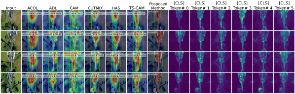
Figure 3: Visualization of test samples from TelDrone. Results of baseline method including TS-CAM shows that these method can only cover some parts of the object and invisible parts are also included in the bounding box due to extensive search of thresholds. In contrast, our method learns to predict map that can cover the whole object. Moreover, maps in red box are used to sample pseudo-labels and our methods learns to localize the object precisely and able remove noise from them.

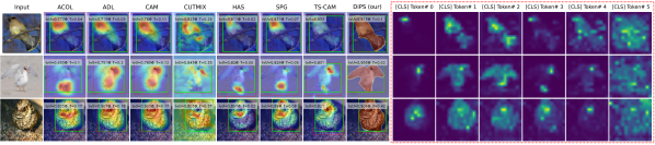
Figure 4: Visualization of test samples from CUB dataset.

where $Y_{i}$ set of all pixel in the generated map,    1 0 .3 1$\mathbb{Y}_{i}^{+}$ represents the top $n\%$ pixels within the bounding box selected through multinomial sampling and    1 0 .3 1$\mathbb{Y}_{i}^{-}$ represents top $-n\%$ pixels anywhere that are derived using uniform sampling from the activations of whole image sorted in reverse order. These pixels are derived from unreliable attention maps and may contain incorrect labels. To deal with this uncertainty, we select only a few (see experimental details for exact values) pixels from the foreground and background while rejecting others [37, 38]. Therefore, the final set of foreground and background pixels for calculating loss are:

$$\varphi(\mbox{\hskip 7.50002pt{1 0 .3 1}\hbox to0.0pt{\hss\leavevmode\hbox{\set@color$\mathbb{Y}$}}}_{i}^{+,-})=\varphi(\mbox{\hskip 9.42929pt{1 0 .3 1}\hbox to0.0pt{\hss\leavevmode\hbox{\set@color$\mathbb{Y}_{i}^{+}$}}})\cup\varphi(\mbox{\hskip 9.42929pt{1 0 .3 1}\hbox to0.0pt{\hss\leavevmode\hbox{\set@color$\mathbb{Y}_{i}^{-}$}}})$$ (4)

here $\varphi(\mbox{\hskip 9.42929pt{1 0 .3 1}\hbox to0.0pt{\hss\leavevmode\hbox{\set@color$\mathbb{Y}_{i}^{+}$}}})$ and $\varphi(\mbox{\hskip 9.36668pt{1 0 .3 1}\hbox to0.0pt{\hss\leavevmode\hbox{\set@color$\mathbb{Y}^{-}$}}})$ represent set of pixels (hyper-parameter) sampled using multinomial distribution. At the end, we then generated pseudo label $Y\in\{0,1\}^{2}$ by assigning 1’s to pixel in    1 0 .3 1$\mathbb{Y}_{i}^{+}$ and 0’s to pixels in set    1 0 .3 1$\mathbb{Y}_{i}^{-}$.

Overall Training Loss: Our training loss consists of three terms; (i) classifier’s loss to ensure the integrity of generated map. The generated map $M_{1}$ is overlaid on the image $x$ and passed it to the classifier to compute a cross-entropy loss; $\mathcal{L}_{CLS}=-\sum_{k=1}^{K}y_{k}log(Softmax(\mbox{\hskip 7.22223pt{1 0 .3 1}\hbox to0.0pt{\hss\leavevmode\hbox{\set@color$\mathrm{C}$}}}{(x\odot M_{1})})_{k})$. (ii) Our constrained pixel alignment loss for learning foreground/background regions. It aligns the output map $M$ with the selected pixels in $\varphi(\mbox{\hskip 7.50002pt{1 0 .3 1}\hbox to0.0pt{\hss\leavevmode\hbox{\set@color$\mathbb{Y}$}}}_{i}^{+,-})$ through partial cross-entropy denoted by $\mathcal{L}_{CPA}(\varphi(\mbox{\hskip 7.50002pt{1 0 .3 1}\hbox to0.0pt{\hss\leavevmode\hbox{\set@color$\mathbb{Y}$}}}_{i}^{\;r}),M^{\;r})$; here $r$ represent the selected pixels. (iii) Conditional Random Field (CRF) [40] to align the localization map with the object boundaries. The detailed description of the CRF loss $\mathcal{L}_{CRF}$ is presented in supplementary material. Furthermore, the overall can be formulated as,

$$\mathcal{L}_{Total}=\min_{\theta}\lambda_{CLS}\mathcal{L}_{CLS}+\lambda_{CPA}\mathcal{L}_{CPA}+\lambda_{CRF}\mathcal{L}_{CRF}$$ (5)

where $\lambda_{CLS}$ and $\lambda_{CPA}$ are hyperparameters between interval [0, 1], and $\lambda_{CRF}$ is set to $2e^{-9}$ as defined in [40].

4 Results and Discussion

4.1 Experimental Methodology

Datasets: For validation, we employed two datasets: CUB-200-2011 and an internal dataset named TelDrone. CUB200-2011 is one of the most popular datasets used for visual classification and object localization tasks. This dataset consists of 11,788 images divided into 200 categories; 5,794 for testing and 5,994 for training [49]. For validation and hyperparameter search, we employed an independent validation set collected by [13] containing 1,000 images. TelDrone contains 915 4K images collected using a drone that orbits around the tower site. Furthermore, images are divided into two classes (either containing an inspection site or not). From this dataset, we considered 797 images for training, 13 images for validation and 105 images as a test set.

Evaluation measures: We analyze our results based on the evaluation measure suggested in [13] – MaxBoxAccV2 refers to the proportion of predicted bounding boxes that have an IoU greater than a particular threshold concerning the generated map. It is averaged over three different IoU thresholds $\delta\in\{30\%,50\%,70\%\}$. We also reported additional localization matrices in supplementary material as presented in [13].

Implementation details: We follow the protocol in [13] for all experiments. A batch size of 32 is used for all datasets. For training on CUB, images are resized to $256\times 256$, and then randomly cropped to $224\times 224$ and randomly flipped horizontally as in [13]. Moreover, for the TelDrone dataset, we first resize images to $512\times 512$ followed by random cropping of size $448\times 448$. We trained our model for 50 epochs while the learning rate is decayed by a factor of 0.1 after every $15^{th}$ epoch for both dataset.

Baseline Models: To evaluate the performance of our model, we compared it with several state-of-the-art methods presented in Tables 1. We report results from [13] for CAM [62], HaS [37], ACoL [59], SPG [60], ADL [14], and CutMix [56]. For all other models, we report the same results as published in their respective articles. For qualitative evaluation, we reproduced the results of CAM [62], HaS [37], ACoL [59], SPG [60], ADL [14], CutMix [56] and TS-CAM [17] according to the protocols defined in [13].

4.2 Comparison with State-of-Art Methods

Table 1 shows that DiPS achieves state-of-the-art performance on CUB and TelDrone datasets for MaxBoxAccV2 metric compared to the other methods in the literature. The visual results of our method along with the corresponding baselines on TelDrone and CUB datasets are presented in Fig.3 and Fig.4 respectively. The baseline method tends to focus on discriminative regions and expands to less discriminative regions because of the bloby nature of these maps. However, the selection of the optimal threshold allows the less discriminative area to be included in the localization map because of their texture or color similarity. Furthermore, the resultant map becomes unreliable and unable to identify the whole object as it encompasses regions with no concealed activation over an object. For CUB dataset, we compare the results with the baseline methods (Fig.4) including TS-CAM and show that our method is capable of covering the whole object with the same intensities instead of highlighting different parts of the object. Additionally, the class tokens of SST are also presented, and DiPS is able to successfully harvest useful information from them by constructing a reliable pseudo-label. Similarly, on the TelDrone dataset, DiPS achieved state-of-the-art visual results by localizing all parts of the object with the same confidence instead of hot-spotting different regions (Fig.3). More specifically, current state-of-the-art methods (e.g. TS-CAM) focus on some regions of the concerned object by hot-spotting different parts. Due to this they are able to properly draw a bounding box around the object due to extensive threshold search that can include low scoring areas to the localization map. In contrast, our method can produce a map that covers the whole object with sharper boundaries, which eliminates the need for a precise threshold value. Additionally, we compare the results of our model with SST’s activation and show that our method learns to localize well even with noisy pseudo-labels.

Methods		TelDrone		CUB
		(MaxBoxAccV2)		(MaxBoxAccV2)
CAM [62] (cvpr,2016)		55.9		63.7
HaS [37] (iccv,2017)		60.3		64.7
ACoL [59] (cvpr,2018)		59.1		66.5
SPG [60] (eccv,2018)		67.3		60.4
ADL [14] (cvpr,2019)		66.0		66.3
CutMix [56] (eccv,2019)		57.2		62.8
ICL [21] (accv,2020)		–		63.1
TS-CAM [17] (iccv,2021)		72.2		76.7
CAM-IVR [23] (iccv,2021)		–		66.9
PDM [28] (tip,2022)		–		72.4
C2AM [52] (cvpr,2022)		–		83.8
ViTOL-GAR [19] (cvpr,2022)		–		72.4
ViTOL-LRP [19] (cvpr,2022)		–		73.1
TRT [39] (corr,2022)		–		82.0
BGC [22] (cvpr,2022)		–		80.1
SCM [3] (eccv,2022)		–		89.9
CREAM [53] (cvpr’22)		–		73.5
F-CAM+CAM [7] (wacv’22)		–		79.4
F-CAM+LayerCAM [7] (wacv’22)		–		80.1
DiPS (ours)		84.9		90.9

Table 1: MaxBoxAccV2 performance on the TelDrone and CUB.

Analysis of distribution shift. We present the effect of varying the threshold values on the localization performance along with the distribution spread of foreground and background regions. The change in MaxBoxAcc at different threshold for CUB test set is presented in Figure 5. We compare our results with CAM [62], HaS [37], ACoL [59], SPG [60], ADL [14], and CutMix [56]. For all of these related methods, we can see that the MaxBoxAcc quickly drops to zero as the threshold increases. Due to this, it is very difficult to find the optimal threshold for each image which makes these methods unfeasible to deploy in practical scenarios. In contrast, the output of our method is less susceptible to the threshold.

Figure 5: MaxBoxAcc performance at different IoU threshold values for output map using the CUB dataset.

5 Conclusion

In this paper, we proposed a DL method for WSOL, capable of producing fine-grained object localization maps of cell tower sites in aerial images for assets surveillance. The proposed method is capable of learning from pseudo-labels instead of only class labels. These pseudo-labels are harvested by sampling foreground and background areas from the class token of an SST. Our method is able to generate better maps compared to the class token used to build pseudo-labels. The proposed method is capable of generating reliable maps, thus providing better coverage of the whole object. To validate the performance of our model, we compared its results with the existing baseline method, and our method achieved competitive performance both qualitatively and quantitatively. Compared to the baseline, our method can identify all parts of the object instead of decomposing and highlighting different parts of the objects. Furthermore, the proposed method eliminates the need for an extensive threshold search to produce an optimal bounding box covering the concerned object.

Note: Additional details are provided in the supplementary materials, including additional visual results, an evaluation matrix for error dissection, an extended error analysis, ablation studies, and an overview of the CRF loss.

Acknowledgments: This research was supported by MITACS and the Natural Sciences and Engineering Research Council of Canada. We also acknowledge Compute Canada for the computing resources.

Appendix A Supplementary Material

This section contains the following material:

1. an evaluation measures and error dissection;

2. an overview of CRF loss;

3. additional error analyses;

4. ablation studies;

5. additional visual results;

6. details on the TS-CAM method.

A.1 Performance Measures and Error Dissection

A.1.1 Evaluation Measure for Error Dissection

In this section, we present the evaluation measures that are used in [17] for error dissection over wrong predictions. These measures are useful for deciding threshold values for producing bounding boxes from localization maps. Specifically, localization part error (LPE) and localization more error (LME) help in deciding whether to increase or decrease the threshold value for optimal results. More details on error measures are given below:

Localization Part Error (LPE): This measure identifies that an object partially detected by the localization map with a large margin has an intersection over the predicted bounding box (IoP) $>$ 0.5.

Localization More Error (LME): It indicates that the predicted bounding box is larger than the actual box and covers other objects or background. This can be identified if intersection over annotated-bounding-box (IoA) $>$ 0.7.

A.1.2 Additional Performance Measures

Top-1 Localization Accuracy (Top-1 Loc): A prediction is considered true if the predicted class is the same as the ground truth and the intersection over Union (IoU) is greater than 0.5.

Top-5 Localization Accuracy (Top-5 Loc): A prediction is considered true if the IoU is greater than 0.5 and the actual class matches at least one of the top 5 predicted classes.

A.2 Overview of CRF loss

Conditional random fields (CRF) loss, aligns the predicted localization map $\mathrm{M}$ with the boundaries of a concerned object presented in input $\mathrm{x}$. CRF loss [40] between $\mathrm{x}$ and $\mathrm{M}$ can be defined as follows:

$$\mathcal{L}_{CRF}(\mathrm{A},\mathrm{M})=\sum_{i=0}^{i=1}{M_{i}}^{T}A(1-M_{i})$$ (A1)

where $\mathrm{A}$ represents an affinity measure that contains mutual similarities between pixels, including proximity and color information. For capturing affinities of pixels, we use a Gaussian kernel [24] and employ permutohedral lattice [1] to reduce the computation overhead.

	LPE $\downarrow$	LME $\downarrow$
VGG16	21.91	10.53
InceptionV3	23.09	5.52
TS-CAM [17]	6.30	2.85
DiPS (our)	0.05	0.07

Table A1: Extended error analysis on the CUB-200-2011 dataset

.

A.3 Extended Error Analysis

Further error analysis (according to the error measures defined in Section A.1.1) on the CUB datasets is presented in Table A1. Our method localized the correct region of the concerned object instead of overestimating or underestimating the region. It also shows that the maps generated by DiPS are very robust and have much fewer errors compared to the baseline methods. The statistics of the baseline methods are from [17].

A.4 Additional Ablation Studies

The performance of DiPS with various loss function combinations is shown in Table A2. It shows that all of the auxiliary losses contribute significantly towards the final performance. Also, training through arbitrary selection of pixels (pseudo-labels) rather than the classifier loss or fixed pseudo-labels allows DL models to explore different regions of an object and can provide accurate localization. Adding CRF and classification terms at the same time significantly improves the performance of our model. The MaxBoxAcc of our model on TelDrone is presented in table A3. Furthermore, the MaxBoxAcc, top-1 and top-5 localization accuracy for CUB dataset is presented in Table A4. We achieved state-of-the-art performance on the TelDrone and CUB dataset.

		CUB		TelDrone
		(MaxBoxAcc)		(MaxBoxAcc)
$\mathcal{L}_{CPA}+\mathcal{L}_{CRF}$		95.4		93.3
$\mathcal{L}_{CPA}+\mathcal{L}_{CLS}$		94.6		91.7
$\mathcal{L}_{CPA}+\mathcal{L}_{CRF}+\mathcal{L}_{CLS}$		97.0		96.2

Table A2: Localization performance of our DiPS method with different losses.

			MaxBoxAcc
CAM [62] (cvpr,2016)			50.9
HaS [37] (iccv,2017)			60.4
ACoL [59] (cvpr,2018)			62.3
SPG [60] (eccv,2018)			67.9
ADL [14] (cvpr,2019)			73.5
CutMix [56] (eccv,2019)			54.7
DiPS (ours)			962

Table A3: MaxBoxAcc performance on the TelDrone dataset.

		CUB
			MaxBoxAcc	top-1 Loc Acc	top-5 Loc Acc
CAM [62] (cvpr,2016)			73.2	56.1	–
HaS [37] (iccv,2017)			78.1	60.7	–
ACoL [59] (cvpr,2018)			72.7	57.8	–
SPG [60] (eccv,2018)			63.7	51.5	–
ADL [14] (cvpr,2019)			75.7	41.1	–
CutMix [56] (eccv,2019)			71.9	54.5	–
ICL [21] (accv,2020)			57.5	–	–
TS-CAM [17] (iccv,2021)			87.7	71.3	83.8
BR-CAM [63] (eccv,2022)			–	–	–
CREAM [53] (cvpr,2022)			90.9	71.7	86.3
BGC [22] (cvpr,2022)			93.1	70.8	88.0
F-CAM [7] (wacv,2022)			92.4	59.3	82.7
DiPS (ours)			97.0	78.8	91.3
DiPS (ours) (w/ TransFG classifier [20])			97.0	88.2	95.6

Table A4: MaxBoxAcc, top-1 and top-5 performance on the CUB dataset.

A.5 Visual Results

Visual representation of our method compared to baseline methods on CUB is illustrated in Fig.A2. Our method generates a very smooth map instead of hot-spotting different parts of the concerned object. Ultimately, the map generated by our method does not require an extensive threshold search to find an optimal bounding box. Compared to the class tokens of SST (used to harvest pseudo-labels), our method is able to learn an effective localization map from noisy pseudo-labels.

A.6 Details on Baseline Method: TS-CAM

By taking advantage of the attention mechanism, TS-CAM [17] is capable of capturing long-range dependency among different parts of an image. As a result, it can efficiently separate background and foreground objects. In other words, it first divides the images into a set of patches for capturing long-range dependency information and records its effects in class token. The attention of class token is then fused with the semantic aware map to produce the final attention/activation map. The flow diagram of TS-CAM is depicted in Fig.A1. Lastly, a detailed visualization of the internal representation of the token TS-CAM class is presented in Fig.A3. It shows that the average of all maps could potentially include noise and background regions in the final prediction.

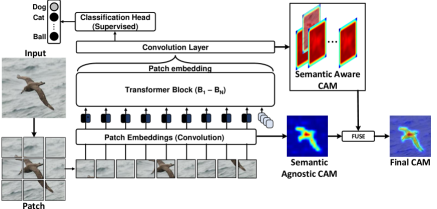
Figure A1: Illustration of the baseline Token Semantic Coupled Attention Map (TS-CAM) model for WSOL.

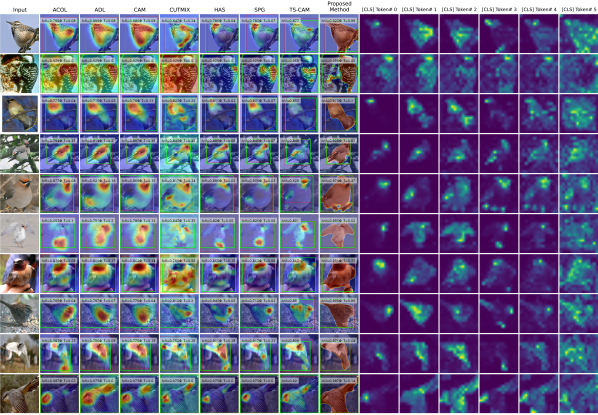
Figure A2: Examples of visual results on the CUB-200-2011 dataset.

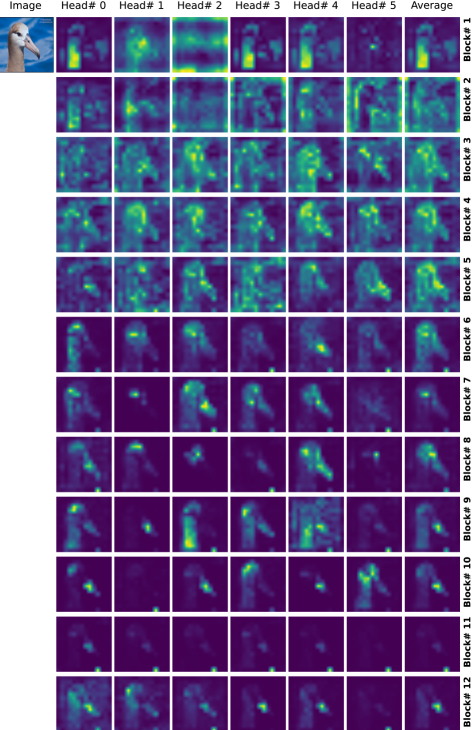
Figure A3: Attention map of each transformer head (class token) learned by TS-CAM. However, different parts of the object are accumulated across the layers/blocks, and it must include semantic aware CAM to suppress noise and generate final results.

References

- [1] Andrew Adams, Jongmin Baek, and Myers Abraham Davis. Fast high-dimensional filtering using the permutohedral lattice. In Computer graphics forum, volume 29, pages 753–762. Wiley Online Library, 2010.
- [2] Christian Allred. 5 major benefits of drone cell tower inspections. in https://thedronelifenj.com/5-major-benefits-of-drone-cell-tower-inspections/, Sep 2022.
- [3] Haotian Bai, Ruimao Zhang, Jiong Wang, and Xiang Wan. Weakly supervised object localization via transformer with implicit spatial calibration. arXiv preprint arXiv:2207.10447, 2022.
- [4] David Bau, Bolei Zhou, Aditya Khosla, Aude Oliva, and Antonio Torralba. Network dissection: Quantifying interpretability of deep visual representations. In Proceedings of the IEEE conference on computer vision and pattern recognition, pages 6541–6549, 2017.
- [5] Soufiane Belharbi, Ismail Ben Ayed, Luke McCaffrey, and Eric Granger. TCAM: Temporal class activation maps for object localization in weakly-labeled unconstrained videos. WACV 2023.
- [6] S. Belharbi, M Pedersoli, I. Ben Ayed, L. McCaffrey, and E. Granger. Negative evidence matters in interpretable histology image classification. In MIDL, 2022.
- [7] S. Belharbi, A. Sarraf, M. Pedersoli, I. Ben Ayed, L. McCaffrey, and E. Granger. F-cam: Full resolution class activation maps via guided parametric upscaling. In WACV, 2022.
- [8] Mathilde Caron, Ishan Misra, Julien Mairal, Priya Goyal, Piotr Bojanowski, and Armand Joulin. Unsupervised learning of visual features by contrasting cluster assignments. arXiv preprint arXiv:2006.09882, 2020.
- [9] M. Caron, H. Touvron, I. Misra, H. Jégou, J. Mairal, P. Bojanowski, and A. Joulin. Emerging properties in self-supervised vision transformers. In ICCV, 2021.
- [10] Aditya Chattopadhay, Anirban Sarkar, Prantik Howlader, and Vineeth N Balasubramanian. Grad-cam++: Generalized gradient-based visual explanations for deep convolutional networks. In 2018 IEEE Winter Conference on Applications of Computer Vision (WACV), pages 839–847. IEEE, 2018.
- [11] Zhiwei Chen, Changan Wang, Yabiao Wang, Guannan Jiang, Yunhang Shen, Ying Tai, Chengjie Wang, Wei Zhang, and Liujuan Cao. Lctr: On awakening the local continuity of transformer for weakly supervised object localization. In Proceedings of the AAAI Conference on Artificial Intelligence, volume 36, pages 410–418, 2022.
- [12] Junsuk Choe, Dongyoon Han, Sangdoo Yun, Jung-Woo Ha, Seong Joon Oh, and Hyunjung Shim. Region-based dropout with attention prior for weakly supervised object localization. Pattern Recognition, 116:107949, 2021.
- [13] Junsuk Choe, Seong Joon Oh, Seungho Lee, Sanghyuk Chun, Zeynep Akata, and Hyunjung Shim. Evaluating weakly supervised object localization methods right. In Proceedings of the IEEE/CVF Conference on Computer Vision and Pattern Recognition, pages 3133–3142, 2020.
- [14] Junsuk Choe and Hyunjung Shim. Attention-based dropout layer for weakly supervised object localization. In Proceedings of the IEEE/CVF Conference on Computer Vision and Pattern Recognition, pages 2219–2228, 2019.
- [15] Alexey Dosovitskiy, Lucas Beyer, Alexander Kolesnikov, Dirk Weissenborn, Xiaohua Zhai, Thomas Unterthiner, Mostafa Dehghani, Matthias Minderer, Georg Heigold, Sylvain Gelly, et al. An image is worth 16x16 words: Transformers for image recognition at scale. arXiv preprint arXiv:2010.11929, 2020.
- [16] Ruigang Fu, Qingyong Hu, Xiaohu Dong, Yulan Guo, Yinghui Gao, and Biao Li. Axiom-based grad-cam: Towards accurate visualization and explanation of cnns. arXiv preprint arXiv:2008.02312, 2020.
- [17] Wei Gao, Fang Wan, Xingjia Pan, Zhiliang Peng, Qi Tian, Zhenjun Han, Bolei Zhou, and Qixiang Ye. Ts-cam: Token semantic coupled attention map for weakly supervised object localization. In Proceedings of the IEEE/CVF International Conference on Computer Vision, pages 2886–2895, 2021.
- [18] Guangyu Guo, Junwei Han, Fang Wan, and Dingwen Zhang. Strengthen learning tolerance for weakly supervised object localization. In Proceedings of the IEEE/CVF Conference on Computer Vision and Pattern Recognition, pages 7403–7412, 2021.
- [19] Saurav Gupta, Sourav Lakhotia, Abhay Rawat, and Rahul Tallamraju. Vitol: Vision transformer for weakly supervised object localization. arXiv preprint arXiv:2204.06772, 2022.
- [20] Ju He, Jie-Neng Chen, Shuai Liu, Adam Kortylewski, Cheng Yang, Yutong Bai, and Changhu Wang. Transfg: A transformer architecture for fine-grained recognition. In Proceedings of the AAAI Conference on Artificial Intelligence, volume 36, pages 852–860, 2022.
- [21] Minsong Ki, Youngjung Uh, Wonyoung Lee, and Hyeran Byun. In-sample contrastive learning and consistent attention for weakly supervised object localization, 2020.
- [22] Eunji Kim, Siwon Kim, Jungbeom Lee, Hyunwoo Kim, and Sungroh Yoon. Bridging the gap between classification and localization for weakly supervised object localization. In Proceedings of the IEEE/CVF Conference on Computer Vision and Pattern Recognition, pages 14258–14267, 2022.
- [23] Jeesoo Kim, Junsuk Choe, Sangdoo Yun, and Nojun Kwak. Normalization matters in weakly supervised object localization. In Proceedings of the IEEE/CVF International Conference on Computer Vision, pages 3427–3436, 2021.
- [24] Vladlen Koltun et al. Efficient inference in fully connected crfs with gaussian edge potentials. Adv. Neural Inf. Process. Syst, 4, 2011.
- [25] Jungbeom Lee, Eunji Kim, Sungmin Lee, Jangho Lee, and Sungroh Yoon. Ficklenet: Weakly and semi-supervised semantic image segmentation using stochastic inference. In Proceedings of the IEEE/CVF Conference on Computer Vision and Pattern Recognition, pages 5267–5276, 2019.
- [26] Ming Li. Caft: Clustering and filter on tokens of transformer for weakly supervised object localization. arXiv preprint arXiv:2201.00475, 2022.
- [27] Meng Meng, Tianzhu Zhang, Qi Tian, Yongdong Zhang, and Feng Wu. Foreground activation maps for weakly supervised object localization. In Proceedings of the IEEE/CVF International Conference on Computer Vision, pages 3385–3395, 2021.
- [28] Meng Meng, Tianzhu Zhang, Wenfei Yang, Jian Zhao, Yongdong Zhang, and Feng Wu. Diverse complementary part mining for weakly supervised object localization. IEEE Transactions on Image Processing, 31:1774–1788, 2022.
- [29] Shakeeb Murtaza, Soufiane Belharbi, Marco Pedersoli, Aydin Sarraf, and Eric Granger. Constrained sampling for class-agnostic weakly supervised object localization. arXiv preprint arXiv:2209.09195, 2022.
- [30] Rakshit Naidu, Ankita Ghosh, Yash Maurya, Soumya Snigdha Kundu, et al. Is-cam: Integrated score-cam for axiomatic-based explanations. arXiv preprint arXiv:2010.03023, 2020.
- [31] Nobuyuki Otsu. A threshold selection method from gray-level histograms. IEEE transactions on systems, man, and cybernetics, 9(1):62–66, 1979.
- [32] Xingjia Pan, Yingguo Gao, Zhiwen Lin, Fan Tang, Weiming Dong, Haolei Yuan, Feiyue Huang, and Changsheng Xu. Unveiling the potential of structure preserving for weakly supervised object localization. In Proceedings of the IEEE/CVF Conference on Computer Vision and Pattern Recognition, pages 11642–11651, 2021.
- [33] Amir Rahimi, Amirreza Shaban, Thalaiyasingam Ajanthan, Richard Hartley, and Byron Boots. Pairwise similarity knowledge transfer for weakly supervised object localization. In Computer Vision–ECCV 2020: 16th European Conference, Glasgow, UK, August 23–28, 2020, Proceedings, Part XXIV 16, pages 395–412. Springer, 2020.
- [34] Harish Guruprasad Ramaswamy et al. Ablation-cam: Visual explanations for deep convolutional network via gradient-free localization. In Proceedings of the IEEE/CVF Winter Conference on Applications of Computer Vision, pages 983–991, 2020.
- [35] O. Ronneberger, P. Fischer, and T. Brox. U-net: Convolutional networks for biomedical image segmentation. In MICCAI, pages 234–241, 2015.
- [36] Ramprasaath R Selvaraju, Michael Cogswell, Abhishek Das, Ramakrishna Vedantam, Devi Parikh, and Dhruv Batra. Grad-cam: Visual explanations from deep networks via gradient-based localization. In Proceedings of the IEEE international conference on computer vision, pages 618–626, 2017.
- [37] Krishna Kumar Singh and Yong Jae Lee. Hide-and-seek: Forcing a network to be meticulous for weakly-supervised object and action localization. In 2017 IEEE international conference on computer vision (ICCV), pages 3544–3553. IEEE, 2017.
- [38] Nitish Srivastava, Geoffrey Hinton, Alex Krizhevsky, Ilya Sutskever, and Ruslan Salakhutdinov. Dropout: a simple way to prevent neural networks from overfitting. The journal of machine learning research, 15(1):1929–1958, 2014.
- [39] Hui Su, Yue Ye, Zhiwei Chen, Mingli Song, and Lechao Cheng. Re-attention transformer for weakly supervised object localization. arXiv preprint arXiv:2208.01838, 2022.
- [40] Meng Tang, Federico Perazzi, Abdelaziz Djelouah, Ismail Ben Ayed, Christopher Schroers, and Yuri Boykov. On regularized losses for weakly-supervised cnn segmentation. In Proceedings of the European Conference on Computer Vision (ECCV), pages 507–522, 2018.
- [41] Hugo Touvron, Matthieu Cord, Matthijs Douze, Francisco Massa, Alexandre Sablayrolles, and Hervé Jégou. Training data-efficient image transformers & distillation through attention. In International Conference on Machine Learning, pages 10347–10357. PMLR, 2021.
- [42] Haofan Wang, Rakshit Naidu, Joy Michael, and Soumya Snigdha Kundu. Ss-cam: Smoothed score-cam for sharper visual feature localization. arXiv preprint arXiv:2006.14255, 2020.
- [43] Haofan Wang, Zifan Wang, Mengnan Du, Fan Yang, Zijian Zhang, Sirui Ding, Piotr Mardziel, and Xia Hu. Score-cam: Score-weighted visual explanations for convolutional neural networks. In Proceedings of the IEEE/CVF Conference on Computer Vision and Pattern Recognition Workshops, pages 24–25, 2020.
- [44] Xiang Wang, Shaodi You, Xi Li, and Huimin Ma. Weakly-supervised semantic segmentation by iteratively mining common object features. In Proceedings of the IEEE conference on computer vision and pattern recognition, pages 1354–1362, 2018.
- [45] Yude Wang, Jie Zhang, Meina Kan, Shiguang Shan, and Xilin Chen. Self-supervised equivariant attention mechanism for weakly supervised semantic segmentation. In Proceedings of the IEEE/CVF Conference on Computer Vision and Pattern Recognition, pages 12275–12284, 2020.
- [46] Jun Wei, Qin Wang, Zhen Li, Sheng Wang, S Kevin Zhou, and Shuguang Cui. Shallow feature matters for weakly supervised object localization. In Proceedings of the IEEE/CVF Conference on Computer Vision and Pattern Recognition, pages 5993–6001, 2021.
- [47] Yunchao Wei, Jiashi Feng, Xiaodan Liang, Ming-Ming Cheng, Yao Zhao, and Shuicheng Yan. Object region mining with adversarial erasing: A simple classification to semantic segmentation approach. In Proceedings of the IEEE conference on computer vision and pattern recognition, pages 1568–1576, 2017.
- [48] Yunchao Wei, Huaxin Xiao, Honghui Shi, Zequn Jie, Jiashi Feng, and Thomas S Huang. Revisiting dilated convolution: A simple approach for weakly-and semi-supervised semantic segmentation. In Proceedings of the IEEE Conference on Computer Vision and Pattern Recognition, pages 7268–7277, 2018.
- [49] P. Welinder, S. Branson, T. Mita, C. Wah, F. Schroff, S. Belongie, and P. Perona. Caltech-UCSD Birds 200. Technical Report CNS-TR-2010-001, California Institute of Technology, 2010.
- [50] Pingyu Wu, Wei Zhai, and Yang Cao. Background activation suppression for weakly supervised object localization. arXiv preprint arXiv:2112.00580, 2021.
- [51] Jinheng Xie, Cheng Luo, Xiangping Zhu, Ziqi Jin, Weizeng Lu, and Linlin Shen. Online refinement of low-level feature based activation map for weakly supervised object localization. In Proceedings of the IEEE/CVF International Conference on Computer Vision, pages 132–141, 2021.
- [52] Jinheng Xie, Jianfeng Xiang, Junliang Chen, Xianxu Hou, Xiaodong Zhao, and Linlin Shen. C2am: Contrastive learning of class-agnostic activation map for weakly supervised object localization and semantic segmentation. In Proceedings of the IEEE/CVF Conference on Computer Vision and Pattern Recognition, pages 989–998, 2022.
- [53] Jilan Xu, Junlin Hou, Yuejie Zhang, Rui Feng, Rui-Wei Zhao, Tao Zhang, Xuequan Lu, and Shang Gao. Cream: Weakly supervised object localization via class re-activation mapping. In Proceedings of the IEEE/CVF Conference on Computer Vision and Pattern Recognition, pages 9437–9446, 2022.
- [54] Haolan Xue, Chang Liu, Fang Wan, Jianbin Jiao, Xiangyang Ji, and Qixiang Ye. Danet: Divergent activation for weakly supervised object localization. In Proceedings of the IEEE/CVF International Conference on Computer Vision, pages 6589–6598, 2019.
- [55] Seunghan Yang, Yoonhyung Kim, Youngeun Kim, and Changick Kim. Combinational class activation maps for weakly supervised object localization. In Proceedings of the IEEE/CVF Winter Conference on Applications of Computer Vision, pages 2941–2949, 2020.
- [56] Sangdoo Yun, Dongyoon Han, Seong Joon Oh, Sanghyuk Chun, Junsuk Choe, and Youngjoon Yoo. Cutmix: Regularization strategy to train strong classifiers with localizable features. In Proceedings of the IEEE/CVF International Conference on Computer Vision, pages 6023–6032, 2019.
- [57] Matthew D Zeiler and Rob Fergus. Visualizing and understanding convolutional networks. In European conference on computer vision, pages 818–833. Springer, 2014.
- [58] Chen-Lin Zhang, Yun-Hao Cao, and Jianxin Wu. Rethinking the route towards weakly supervised object localization. In Proceedings of the IEEE/CVF Conference on Computer Vision and Pattern Recognition, pages 13460–13469, 2020.
- [59] Xiaolin Zhang, Yunchao Wei, Jiashi Feng, Yi Yang, and Thomas S Huang. Adversarial complementary learning for weakly supervised object localization. In Proceedings of the IEEE conference on computer vision and pattern recognition, pages 1325–1334, 2018.
- [60] Xiaolin Zhang, Yunchao Wei, Guoliang Kang, Yi Yang, and Thomas Huang. Self-produced guidance for weakly-supervised object localization. In Proceedings of the European conference on computer vision (ECCV), pages 597–613, 2018.
- [61] Xiaolin Zhang, Yunchao Wei, and Yi Yang. Inter-image communication for weakly supervised localization. In Computer Vision–ECCV 2020: 16th European Conference, Glasgow, UK, August 23–28, 2020, Proceedings, Part XIX 16, pages 271–287. Springer, 2020.
- [62] Bolei Zhou, Aditya Khosla, Agata Lapedriza, Aude Oliva, and Antonio Torralba. Learning deep features for discriminative localization. In Proceedings of the IEEE conference on computer vision and pattern recognition, pages 2921–2929, 2016.
- [63] Lei Zhu, Qian Chen, Lujia Jin, Yunfei You, and Yanye Lu. Bagging regional classification activation maps for weakly supervised object localization. arXiv preprint arXiv:2207.07818, 2022.
- [64] Lei Zhu, Qi She, Qian Chen, Xiangxi Meng, Mufeng Geng, Lujia Jin, Zhe Jiang, Bin Qiu, Yunfei You, Yibao Zhang, et al. Background-aware classification activation map for weakly supervised object localization. arXiv preprint arXiv:2112.14379, 2021.