Dimension matters when modeling network communities in hyperbolic spaces

Abstract

Over the last decade, random hyperbolic graphs have proved successful in providing geometric explanations for many key properties of real-world networks, including strong clustering, high navigability, and heterogeneous degree distributions. These properties are ubiquitous in systems as varied as the internet, transportation, brain or epidemic networks, which are thus unified under the hyperbolic network interpretation on a surface of constant negative curvature. Although a few studies have shown that hyperbolic models can generate community structures, another salient feature observed in real networks, we argue that the current models are overlooking the choice of the latent space dimensionality that is required to adequately represent clustered networked data. We show that there is an important qualitative difference between the lowest-dimensional model and its higher-dimensional counterparts with respect to how similarity between nodes restricts connection probabilities. Since more dimensions also increase the number of nearest neighbors for angular clusters representing communities, considering only one more dimension allows us to generate more realistic and diverse community structures.

I Introduction

When one pictures a system and relationships between its constituents, the idea of closeness naturally comes to mind because more often than not, the flows that make up those relationships depend upon some form of proximity. Take neurons in a brain or servers underlying the infrastructure of the Internet, two systems that may seem to have little in common. Yet, both are remarkably complex and adequately modeled in the field of network geometry Boguñá et al. (2010); Allard and Serrano (2020); Boguñá et al. (2021), where closeness between nodes and properties of an underlying abstract space explain how elements of the network are interconnected. In particular, a latent space of constant negative curvature, the two-dimensional hyperbolic plane, captures in a simple yet accurate way many significant complex network properties, namely sparsity, self-similarity, small-worldness, heterogeneity, non-vanishing clustering, and community structure Boguñá et al. (2020).

In this framework, each node exists on a surface where a radial dimension encodes its popularity, or how likely it is to have many neighbors, and an angular dimension encodes the similarity between nodes as attractiveness, such that similar nodes are more likely to be related independently of their popularity Papadopoulos et al. (2012). The successes of hyperbolic network geometry cover a wide range of practical applications, like predicting economic patterns across time García-Pérez et al. (2016), making sense of the resilience of the Internet Boguñá et al. (2010) or modeling information flow in the brain Allard and Serrano (2020); Zheng et al. (2019), to name a few. Furthermore, hyperbolic space is the only known metric space on which maximum-entropy random graphs can reproduce real network properties like clustering, sparsity, and heterogeneous degree distributions all at once Boguñá et al. (2020). The model has also been extended to weighted Allard et al. (2017), growing Papadopoulos et al. (2012); Krioukov et al. (2012), bipartite Kitsak et al. (2017), multilayer Kleineberg et al. (2016, 2017) or modular networks García-Pérez et al. (2018); Zuev et al. (2015); Muscoloni and Cannistraci (2018).

Now that hyperbolic networks of the lowest dimension have been shown to capture so many realistic properties, some attention has shifted to the study of higher-dimensional models Yang and Rideout (2020); Almagro et al. (2022); Kovács et al. (2022); Budel et al. (2023). In these, there is still one radial coordinate for popularity, but there are $D>1$ dimensions encoding similarity, or perhaps, similarities. In other words, higher-dimensional hyperbolic network models embody the intuition that there is more than one way in which things can be similar or not. The choice of dimension is an already prominent problem for machine learning applications of hyperbolic embeddings Gu et al. (2021), yet is has mostly been overlooked until recently for hyperbolic network models. In recent works, increasing the dimension was convoluted with the effect of other parameters and studied only at the local scale of node pairs connectivity and expected degrees Yang and Rideout (2020); Kovács et al. (2022); Budel et al. (2023). These studies also found that similar power-law degree distributions can be achieved in any dimensions, by tuning the choice of model’s parameter regime.

These observations involve extremely local properties, concerning nodes and their direct neighbors. As soon as we start zooming out towards the mesoscale level, dimension seems to impact network topology, yet it has not been studied much so far. The maximum clustering coefficient that can be achieved in random geometric graphs, which quantifies the closure of triplets of nodes into triangles, decreases with the dimension García-Pérez et al. (2018); Kovács et al. (2022); Budel et al. (2023). Almagro et al. Almagro et al. (2022) have shown using the short cycle structure that various networked data sets have an underlying hyperbolic dimension that is ultra-low, albeit not minimal as previously assumed. Our work follows this line of research by looking at this question through the lens of community structure.

One of the most ubiquitous properties of complex networks is community structure, when connectivity within subgroups of nodes, or communities, is prominently different than with the rest of the network Girvan and Newman (2002); Cherifi et al. (2019). Network motifs have long been recognized as universal building blocks of complex networks Milo et al. (2002), community structure detection is one of the most long-standing active fields of network science Fortunato and Hric (2016); Fortunato and Newman (2022), and most networked data show some sort of community structure, with one of the most interesting complex systems, the brain, making no exception Betzel et al. (2017, 2019). In hyperbolic network models, community structure is expressed as subgroups of nodes that are closer with respect to their angular coordinates, either in hyperbolic embeddings of real networks Boguñá et al. (2010); García-Pérez et al. (2019) or synthetic models that explicitly generate communities Zuev et al. (2015); García-Pérez et al. (2018); Muscoloni and Cannistraci (2018). Since changing the dimension of hyperbolic network models affects primarily the number of angular coordinates, dimension and community structure are much closer than they appear. In our work, we explore this interplay to see how dimension can improve current modeling of community structure in the hyperbolic framework, but also how community structure offers some insight about the underlying hyperbolic dimension of networks.

Let us take a look at a hyperbolic embedding of the airport network in Fig. 1. Airports within the same continent are more prone to be connected by direct flights, which is why nodes of the same color are mostly grouped by angular coordinate. Nevertheless, airports in Africa, Asia, and Europe seem to be more mixed together because their actual geographic location has, very broadly, the shape of a triangle which cannot be reflected in the maximum likelihood embedding of Fig. 1. This phenomenon is also notable in structural brain networks hyperbolic embeddings of Ref. Allard and Serrano (2020), where neuroanatomical clusters are not all grouped by angular coordinates. These examples illustrate that a unique similarity dimension might not be enough to model community structure with non-sequential patterns. If that were the case, one could wonder why is that so, and how can we quantify community structure in hyperbolic random graphs?

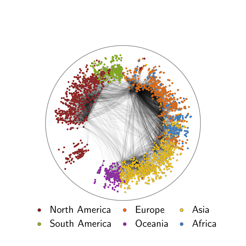
Figure 1: Airports network embedded in the hyperbolic disk using the Mercator algorithm García-Pérez et al. (2019). Edges represent pairs of airports connected by a direct flight and colors represent the continent on which the airport is located. Here, edges follows hyperbolic geodesics of the conformal disk model Ratcliffe (2006). Data downloaded from openflights.org.

As to why, we find that going from one angular similarity dimension to more, and even to only one more, have drastic effects on how the similarity between nodes influences their connectivity. We show that angular closeness constrains connections much more, and differently, in $D=1$ than in other dimensions, which is done by studying the probability density function of the angular distance between connected nodes. We also quantify how the number of neighbors is not the same on a circle or on a sphere or on an even higher-dimensional sphere. This phenomenon impacts the number of nearest neighbors for angular clusters representing communities in hyperbolic random graphs. As a simplest experiment of how those two phenomenons come into play, we generate hyperbolic networks possessing community structure in ${D=1}$ and ${D=2}$. We thus obtain insights into how and why networks with community structure might have an underlying hyperbolic dimension that is higher than one.

The paper is structured as follows. In Sec. II, the key properties of the $\mathbb{H}^{D+1}$ hyperbolic random graph model are recalled, along with its relationship to the $\mathbb{S}^{D}$ formulation and some remarks about angular distance on $D$-spheres. The interplay between distance and dimension is studied in Sec. III, where we will see how dimension affects how connected nodes in hyperbolic random graphs are likely to be found at a given angular distance from one another. In either the pairwise case, where the expected degrees of the nodes have to be considered, or in the general case, for any expected degree distribution, the probability of finding connected nodes at a certain angular distance presents a sharp contrast between $D=1$ and $D\geq 2$. Then, we digress briefly on the number of neighbors on $D$-spheres. In the last part of the paper, we show how this affects the possibility to generate hyperbolic networks with community structure. This is quantified on block matrices representing how the generated communities are related to one another in Sec. IV.

II Hyperbolic networks model

We first review basic notions and establish some useful notation about hyperbolic random graphs in any dimension, before presenting some of their most remarkable properties.

A hyperbolic space is a complete, simply connected, Riemannian manifold of constant negative curvature $-\zeta^{2}$ and dimension $D+1$ (Ratcliffe, 2006, Chap. 8)Myers (1935). The lowest dimensional space with $D=1$ is the hyperbolic plane, a smooth surface that can be modeled as one sheet of a hyperboloid in the three-dimensional Minkowski space, but also using other equivalent models like the upper half-plane, the Klein disk and the Poincaré disk Ratcliffe (2006); Stillwell (1996).

Hyperbolic random graphs are based upon the hyperboloid model $H^{2}$, where all points of the hyperbolic plane are parametrized using coordinates $\varphi\in[0,\,2\pi)$ and $r\in[0,{R})$ and thus have a natural projection on a circle through coordinate $\varphi$ Krioukov et al. (2010). An analogous coordinate parametrization is used in higher dimension. The angular coordinate then map points to the $D$-sphere instead of the circle, i.e. $\varphi=(\varphi_{1},...,\varphi_{D})$, with $\varphi_{1},...,\varphi_{D-1}\in[0,\pi)$ and $\varphi_{D}\in[0,2\pi)$ Yang and Rideout (2020)(Ratcliffe, 2006, Sec. 3.4). The distance $d_{h}$ between two points $x,x^{\prime}\in H^{D+1}$ whose respective coordinates are $(\varphi,r)$ and $(\varphi^{\prime},r^{\prime})$ is given by the hyperbolic law of cosines,

$$d_{h}(x,x^{\prime})=\frac{1}{\zeta}\mathrm{arcosh}(\cosh\zeta r\cosh\zeta r^{\prime}\\ -\sinh\zeta r\sinh\zeta r^{\prime}\cos\theta),$$ (1)

where $\zeta\in(0,\infty)$ is related to the hyperboloid’s curvature $-\zeta^{2}$ and $\theta=\acos(\nicefrac{{x\cdot x^{\prime}}}{{|x|\,|x^{\prime}|}})$ is the angular distance between $x$ and $x^{\prime}$, here considered as two vectors in $\mathbb{R}^{D+1}$. This generalization is referred to as the hyperboloid model $H^{D+1}$. One important aspect of Eq. (1) is that, for sufficiently large $r,r^{\prime}$, and for small $\theta$,

$$d_{h}(x,x^{\prime})\approx r+r^{\prime}+\frac{2}{\zeta}\log\biggl(\frac{\theta}{2}\biggr{missing}),$$ (2)

where the first expression becomes exact in the large network limit and the last expression holds for small $\theta$. This approximation was first published in Ref. Krioukov et al. (2010), but one can also refer to Refs. Yang and Rideout (2020); Alanis-Lobato and Andrade-Navarro (2016) for more detailed derivations and bounds on the approximation.

What is referred to as the $\mathbb{H}^{D+1}$ model throughout this paper is not only the hyperbolic space presented above, but a random graph defined on this space. Consider a set of $N$ nodes, $V=\{x_{i}\}_{i=1,\ldots,N}\subset H^{D+1}$, where each $x_{i}$ is a continuous random variable on $H^{D+1}$. A natural choice to study the effect of hyperbolic geometry on the graph is to sample uniformly in a subset of $H^{D+1}$, but most models can also generate networks with other node densities on the hyperbolic disk, which is reflected in the diversity of possible node degree distributions that have been studied Serrano et al. (2008); Krioukov et al. (2010); Yang and Rideout (2020). The connection probability

$$p_{h}(x,x^{\prime})=\frac{1}{1+e^{\beta\zeta[d_{h}(x,x^{\prime})-{\mu}]/2}}$$ (3)

defines a random graph with node set $V$, where each edge is an independent Bernoulli random variable with chance of success $p_{h}(x,x^{\prime})$. We stress that there are two levels of randomness. First, the nodes’ positions are sampled from a continuous distribution on $H^{D+1}$. Second, each realization of those positions defines a discrete probability measure on the set of all simple graphs of size $N$. For uniformly distributed nodes, shortest paths on graphs sampled from $\mathbb{H}^{2}$ follow the shortest paths on the underlying hyperbolic space $H^{2}$ with high probability, a phenomenon first observed in Boguñá and Krioukov (2009); Krioukov et al. (2010). This phenomenon is referred to as hyperbolic routing or congruence between the graphs and their underlying space Boguñá et al. (2021), and is yet to be studied in $D>1$.

Two additional parameters are introduced in Eq. (3): ${\mu}>0$ that sets a connectivity distance threshold and tunes the expected average degree when nodes are sampled uniformly Krioukov et al. (2010) and $\beta>0$ that controls for the range of connection probabilities. Akin to the phase transition at $\beta=1$ in the original model Krioukov et al. (2010), there is a phase transition at $\nicefrac{{\beta}}{{D}}=1$, a critical value for which uniform hyperbolic random graphs have different average expected degree and power-law exponent of the degree distribution, in the asymptotic limit of large graphs Budel et al. (2023); van der Kolk et al. (2021); Kovács et al. (2022). Our work takes place in the so-called “cold” regime, $\beta>D$, which has been shown to generate graphs with power-law degree distributions and low average degree. It also follows that the ratio $\nicefrac{{\beta}}{{D}}$ is kept constant when comparing models of different dimensions in Secs. III and IV, in order to study different dimensions in the same asymptotic regime.

With the model now explicitly defined, let us now take at closer look at which node properties the radial and angular coordinates abstract. As mentioned in the introduction, the radial coordinate encodes nodes popularity since the closer a node is to the center of the hyperbolic ball, the higher its expected degree will be Krioukov et al. (2010); Papadopoulos et al. (2012). The angular coordinates abstract an ensemble of similarity attributes, properties of the data underlying the network that drive nodes to be connected or not, independently of their degree. Those attributes do not have to be known explicitly, and can be related in a non-trivial way, in a manner reminiscent of how some data can be abstracted by principal components or eigenvectors. This is why detecting how many similarity dimensions would be needed to adequately model a given networked dataset is of research interest Almagro et al. (2022); Gu et al. (2021).

The random graph model can also be defined in the $\mathbb{S}^{D}$ representation Serrano et al. (2008), using the same angular coordinates that maps the nodes to a $D$-sphere ${S^{D}=\{x\in\mathbb{R}^{D+1}\,|\,|x|^{2}=\hat{R}^{2}\}}$, but assigning to each node a new continuous random variable, the latent degree $\kappa\in(\kappa_{0},\infty)$, instead of the radial coordinate $r$. The following change of variables, a $D$-dimensional generalization of what was first done in Krioukov et al. (2009, 2010), transforms from $r$ to $\kappa$ and inversely through

$$\kappa=\kappa_{0}\exp[\frac{\zeta D}{2}({R}-r)\biggr{]}.$$ (4)

In $D=1$, this simple mapping has been reinstated regularly over the last decade to highlight the correspondence between both models García-Pérez et al. (2019); Boguñá et al. (2021), yet to the best of our knowledge it had not been previously published in arbitrary dimension. Introducing one last parameter $\hat{\mu}$, we can set ${{\mu}=(\nicefrac{{2}}{{\zeta}})\log[\nicefrac{{2\hat{R}}}{{(\hat{\mu}\kappa_{0}^{2})^{1/D}}}]}$ in Eq. (3) and using the hyperbolic distance approximation of Eq. (2), we obtain

$$p_{s}(x,x^{\prime})=\frac{1}{1+\left[\frac{\hat{R}\theta}{(\hat{\mu}\kappa\kappa^{\prime})^{\nicefrac{{1}}{{D}}}}\right]^{\beta}},$$ (5)

the connection probability as originally defined in the latent variables formalism Serrano et al. (2008). Albeit having different values for the equivalence between connection probabilities to hold, parameters $\hat{R}$ and $\hat{\mu}$ in the $\mathbb{S}^{D}$ model play a similar role, respectively with regards to nodes’s density on the space and the mean degree, as $R$ and $\mu$ in the $\mathbb{H}^{D+1}$ model, which justifies this choice of notation .

For large sparse graphs with uniformly sampled angular coordinates, the parameter $\hat{\mu}$ can be tuned such that the expected degree of a node with latent degree $\kappa$ (sampled from any distribution) is proportional to the value of $\kappa$ Serrano et al. (2008); García-Pérez (2018), where the expectation is over all possible realizations of $\mathbb{S}^{D}$, hence the name “latent degree”. In addition to this relation between latent and expected degrees, Eq. (5) highlights how angular coordinates encode similarity and latent degrees encode popularity, since the connection probability gets closer to 1 for small angular distance $\theta$ and high latent degrees $\kappa,\kappa^{\prime}$. For this reason, the $D$-sphere parameterized by angular coordinates is sometimes referred to as the similarity space. It is worth mentioning that in the literature, the notation is often simplified by adequately fixing parameters, which has not been done heretofore to keep the relationship between cited articles more accessible.

The change of variables defined in Eq. (4) preserves the connection probabilities between nodes whenever Eq. (2) is valid. For uniformly distributed nodes on a ball of $H^{D+1}$, it has been shown that the proportion of node pairs for which this is true tends to 1 Boguñá et al. (2021). Thus, random graph models within either $\mathbb{S}^{D}$ or $\mathbb{H}^{D+1}$ are considered equivalent. In our work the $\mathbb{S}^{D}$ representation is used without loss of generality.

Given latent degrees $\kappa,\kappa^{\prime}$, we can define a new continuous random variable,

$$\eta(\kappa,\kappa^{\prime}):=\frac{(\hat{\mu}\kappa\kappa^{\prime})^{\nicefrac{{1}}{{D}}}}{\hat{R}},$$ (6)

whose outcome depends on the probability density function (pdf) of latent degrees, as well as parameters $\hat{\mu}$ and $\hat{R}$. Letting go of the explicit dependency on $\kappa\kappa^{\prime}$ for brevity, the connection probability between a pair of nodes, given by Eq. (5), can be written as

$$p(\theta,\eta)=\frac{1}{1+(\theta/\eta)^{\beta}},$$ (7)

which highlights that $\eta$ acts as a local angular distance connectivity threshold. Indeed,

$$\lim_{\beta\to\infty}p(\theta,\eta)=H(\eta-\theta),$$ (8)

where $H$ is the Heaviside step function. Thus, in the $\beta\to\infty$ regime, all node pairs for which $\theta<\eta$ would be connected. In the $\mathbb{S}^{D}$ representation, it is common to fix the radius $\hat{R}$ such that the number of nodes $N$ is equal to the surface area of the $D$-sphere Serrano et al. (2008); García-Pérez et al. (2019), which yields a node density of 1 with

$$\hat{R}=\quantity(\frac{\Gamma(\frac{D+1}{2})N}{2\pi^{\nicefrac{{(D+1)}}{{2}}}})^{\nicefrac{{1}}{{D}}}.$$ (9)

In this setting, $\eta$ varies as $(\nicefrac{{\kappa\kappa^{\prime}}}{{N}})^{1/D}$. Thus, we can think of $\eta$ as capturing the pairwise popularity in a way reminiscent of how the angular distance $\theta$ captures the similarity of node pairs.

A common choice of pdf for angular coordinates is such that points parametrized by $\varphi$ are uniformly distributed on $S^{D}$. For latent degrees, we consider a Pareto distribution with mean $\bar{\kappa}$,

$$f_{K}^{\mathrm{Pareto}}(\kappa)=(\gamma-1)\,\kappa_{0}^{\gamma-1}\kappa^{-\gamma},\qquad\kappa_{0}=\frac{\bar{\kappa}(\gamma-2)}{\gamma-1},$$ (10)

which, with ${\gamma=2\zeta+1}$, is akin to sampling nodes uniformly from a hyperbolic ball of $H^{D+1}$, but offer more freedom on the shape of the degree distribution.

Increasing the dimension of spheres is far from being as intuitive as unfolding more dimensions of flat spaces. Let us picture this using angular distance distributions on $D$-spheres. Let $X$ be a random variable describing the angular distance $\theta\in[0,\pi]$ between two points sampled uniformly at random on $S^{D}$. As derived in Cai et al. (2013), the pdf of $X$ is given by

$$f_{X}(\theta)=\frac{1}{I_{D}}\sin^{D-1}\theta,$$ (11)

with

$$I_{D}=\int_{0}^{\pi}\sin^{D-1}\theta\,\differential\theta=\frac{\Gamma(\nicefrac{{D+1}}{{2}})}{\sqrt{\pi}\,\Gamma(\nicefrac{{D}}{{2}})}.$$ (12)

Figure 2 shows that for $D\gg 1$, chances are that any other point will be found at more or less an angular distance of $\theta=\nicefrac{{\pi}}{{2}}$, a surprising property related to the concentration of measure phenomenon Ledoux (2001). Yet even for very low $D$, there is a significant qualitative shift between uniformity in $D=1$ and unimodality in $D\geq 2$. This well-known property hints intuition for the upcoming section, where instead of sampling pairs of points on $D$-spheres, we study edges of hyperbolic random graphs.

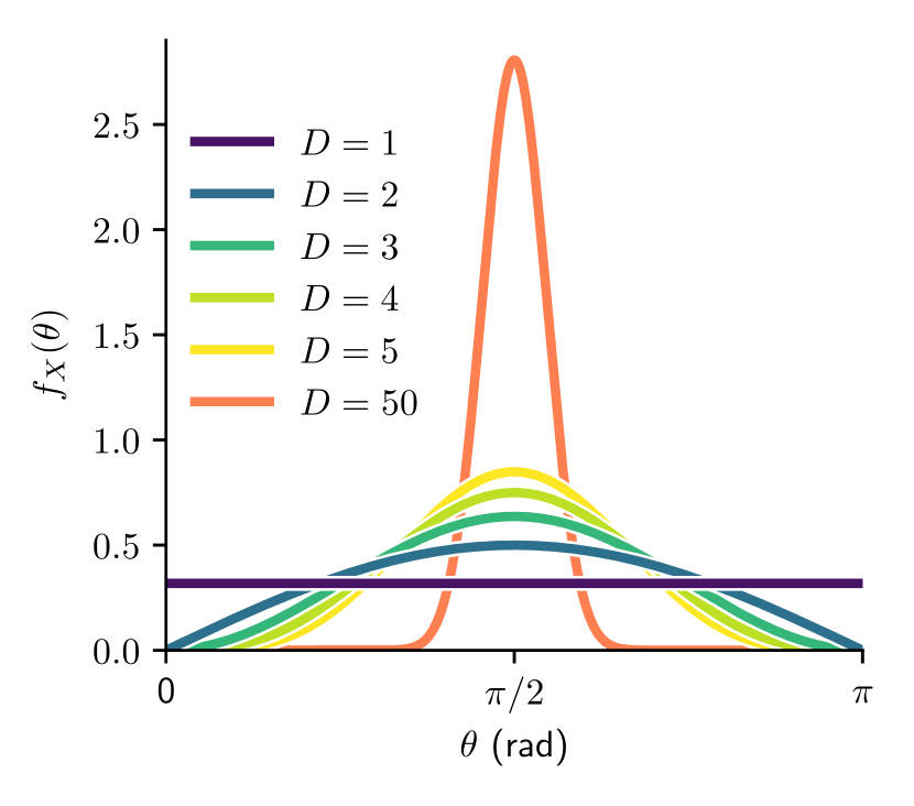
Figure 2: Probability density function of angular distance between points sampled uniformly at random on a $D$-sphere.

III Effects of dimensionality

Dimension is a fundamental property of spaces. An ant living on a circle would have much less freedom than one living on a sphere. Yet, if those two ants were to talk to each other, they might agree that they live on the same kind of space because some properties, like the possibility to come back to the same point by going straight ahead long enough, are the same. As presented in Sec. II, increasing the dimension of hyperbolic random graphs boils down to considering more angular coordinates that map to the sphere or higher dimensional $D$-spheres, but how does this impact the graph structure? Some properties of the graphs are almost unchanged, like the degree distribution Yang and Rideout (2020), while some others, like the short cycle structure Almagro et al. (2022), are affected significantly.

Our take on this question broadly deals with neighborhoods, of connected nodes in the graph but also simply of points on $D$-spheres. Since the dimension affects primarily the angular similarity space, the focus is first on uniform distribution of nodes on $\mathbb{S}^{D}$ and the study of angular distance between nodes that are connected. On another note, we then study how the number of nearest neighbors on $D$-spheres varies with dimension.

III.1 Angular distance between connected nodes

In $\mathbb{S}^{1}$, most edges are observed between nodes separated by a very small angular distance, except for nodes of very high expected degree (see for instance (Krioukov et al., 2010, Fig. 5.)). We have found this propriety to change with the dimension of the underlying hyperbolic space. This is to be expected since the probability to find any other node at a very close angular distance decreases with dimension, as shown in Fig. 2. Yet, this effect of dimensionality has interesting consequences on hyperbolic random graphs, especially when comparing $D=1$ and $D>1$.

Consider a $\mathbb{S}^{D}$ model of $N$ nodes as defined in Sec. II with angular coordinates sampled uniformly with respect to the spherical measure and latent degrees sampled from any pdf $f_{K}(\kappa)$. We study the distribution of the angular distance between connected nodes within this hyperbolic random graph, as a way to assess the interplay between the dimension of the similarity space and the topology of the graph. A pairwise case of two nodes with given latent degrees is first examined, then its generalization to the whole latent degree distribution. The hard threshold limit described by Eq. (8) is also studied since it allows for some insightful approximations of our results.

III.1.1 For a pair of nodes, general case

Consider a pair of nodes with latent degrees $\kappa,\kappa^{\prime}$ such that $\eta$ is given by Eq. (6). We study the pdf of angular distance between those two nodes, provided that they are connected in the random graph. Let $X$ be the continuous random variable describing the angular distance $\theta\in[0,\pi]$ between these nodes. Since the angular coordinates of the graph are uniformly distributed, the pdf of $X$ is given by Eq. (11). Let $Y$ be the continuous random variable describing the value of $\eta$, whose support depends on possible values of $\kappa$. Finally, let $A$ be the discrete Bernoulli random variable describing whether the nodes are connected ($A=1$) or not ($A=0$) according to the probability of Eq. (5). The pdf of angular distance between two nodes is given by the conditional pdf

$$f_{X|Y,A}(\theta\,|\,\eta,\,1)=\frac{f_{X,Y,A}(\theta,\eta,1)}{f_{Y,A}(\eta,1)}$$ (13)

with the left-hand side notation standing more compactly for $f_{X|Y,A}(X=\theta\,|\,Y=\eta,\,A=1)$. Since $A$ depends on $\theta$ and $\eta$ through the connection probability of Eq. (5), but random variables are otherwise independent, the numerator of Eq. (13) is given by

$$f_{X,Y,A}(\theta,\eta,1)=\frac{f_{X}(\theta)f_{Y}(\eta)}{[1+(\nicefrac{{\theta}}{{\eta}})^{\beta}]}.$$ (14)

Likewise, the denominator is

$$f_{Y,A}(\eta,1)=f_{Y}(\eta)f_{A|Y}(1\,|\,\eta)$$ (15)

where $f_{A|Y}(1\,|\,\eta)$ is the following density, with $X$ marginalized out,

$$f_{A|Y}(1\,|\,\eta)=\int_{0}^{\pi}\frac{f_{X}(X)}{1+(\nicefrac{{\theta}}{{\eta}})^{\beta}}\differential\theta\\ =\int_{0}^{\pi}\frac{\sin^{D-1}\theta}{I_{D}[1+(\nicefrac{{\theta}}{{\eta}})^{\beta}]}\differential\theta.$$ (16)

Altogether, this yields the explicit expression for Eq. (13)

$$f_{X|Y,A}(\theta\,|\,\eta,\,1)=\frac{1}{\mathcal{Z}(\eta)}\frac{\sin^{D-1}\theta}{[1+(\nicefrac{{\theta}}{{\eta}})^{\beta}]},$$ (17)

with normalization

$$\mathcal{Z}(\eta):=\int_{0}^{\pi}\frac{\sin^{D-1}\theta}{1+(\nicefrac{{\theta}}{{\eta}})^{\beta}}\differential\theta.$$ (18)

Intuitively, Eq. (17) is proportional to $\sin^{D-1}\theta$ as in the distance distribution for uniformly distributed nodes on $\mathbb{S}^{D}$ of Eq. (11), while allowing for the influence of hyperbolic connection probability given by Eq. (7). Its behavior for $D\in\{1,2,3,4,5\}$ is shown in Fig. 3, where for all dimensions the expected degree of nodes is kept the same. In Fig. 3 and Fig. 4, we have set $\nicefrac{{\beta}}{{D}}=3.5$ without loss of generality, since our results are not qualitatively affected by this parameter choice, as long as $\nicefrac{{\beta}}{{D}}>1$.

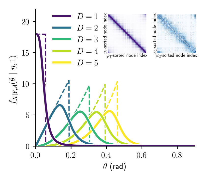
Figure 3: Probability density functions of angular distance between connected nodes in the $\mathbb{S}^{D}$ model given by Eq. (17), for $N=1000$ nodes, with $\kappa=\kappa^{\prime}=10.0$ and $\nicefrac{{\beta}}{{D}}=3.5$. The dashed lines show the $\beta\to\infty$ limit. Inset illustrates $\mathbb{S}^{D}$ connection probability matrices for $D=1$ (left) and $D=2$ (right), $\kappa_{i}=10.0$ for all nodes $i$. The node indices were sorted to satisfy $i<j$ when $\varphi_{D}(i)<\varphi_{D}(j)$, where $\varphi_{D}(i)$ denotes the coordinate $\varphi_{D}\in[0,2\pi)$ of the $i$-th node on the $D$-sphere.

For $D=1$, the maximum is at $\theta=0$, as depicted in the inset by the purple example connectivity matrix , where the dark diagonal line illustrates all of the connection probability concentrated to very small angular distances. The pdf of the angular distance separating connected nodes is strictly decreasing for ${D=1}$ and ${\beta<\infty}$, since it is proportional to the connection probability of Eq. (5). Hence, most edges will have nearly ${\theta=0}$ in ${D=1}$, as expected in the $\mathbb{H}^{2}$ generative model Krioukov et al. (2010) and shown by the purple curve in Fig. 3. By contrast, for $D>1$, this is relaxed, as exemplified by the blue curve and connectivity matrix for $D=2$.

Eq. (17) is unimodal for all $D>1$, with a mode greater than zero and increasing with dimension. The existence and the location of the mode of Eq. (17) for ${D>1}$ is deduced by setting its first derivative with respect to $\theta$ to zero to obtain

$$(D-1)\quantity[\quantity(\frac{\eta}{\theta^{*}})^{\beta}+1]=\frac{\beta\tan\theta^{*}}{\theta^{*}},$$ (19)

where ${\theta^{*}\in(0,\pi)}$ can be a maximum, a minimum or an inflection point. Since Eq. (17) is the product of a unimodal function and a decreasing function, we assume the critical point above is a maximum. It is shown in Appendix A that $\theta^{*}=0$ iff $D=1$. Furthermore, if $\theta^{*}\ll 1$ such that $\tan\theta^{*}\approx\theta^{*}$, the solution of Eq. (19) can be closely approximated by

$$\theta^{*}\approx\eta\quantity(\frac{1}{\frac{\beta}{(D-1)}-1})^{\nicefrac{{1}}{{\beta}}}.$$ (20)

This approximation is valid whenever the angular threshold ${\eta\sim(\kappa\kappa^{\prime}/N)^{\nicefrac{{1}}{{D}}}}$ is small enough, which is the case for a significant fraction of node pairs in hyperbolic random graphs Krioukov et al. (2010) and most observed degree distributions Voitalov et al. (2019). Both factors of Eq. (20) are increasing functions of the dimension $D$. Therefore, for the vast majority of nodes having a “reasonable” expected degree, the most likely angular distance between connected nodes in $\mathbb{S}^{D}$ is greater and greater as dimension increases. This is yet another indicator that most connected nodes will in fact be separated by an angular distance $\theta>0$ in hyperbolic random graphs $\mathbb{S}^{D}$ with $D>1$. The expression (17) encapsulates in a simple yet accurate way that the joint effect of nodes’ angular distribution on $D$-spheres with the hyperbolic connection probability is qualitatively and quantitatively different across ultra-low dimensions of the model.

III.1.2 For a pair of nodes, hard threshold limit

An informative limiting case for the angular distance between connected nodes arises with $\beta\to\infty$. Then, the connection probability becomes a step function given by Eq. (8) with angular distance threshold $\eta$. Equation (17) becomes

$$f_{X|Y,A}(\theta\,|\,\eta,1)\overset{\beta\to\infty}{\approx}\frac{H(\eta-\theta)\sin^{D-1}\theta}{\mathcal{Z}(\eta)}\\ \overset{\eta\ll 1}{\approx}\frac{H(\eta-\theta)\,D\theta^{D-1}}{\eta^{D}},$$ (21)

where the second approximation uses the small angle property of sine. In Fig. 3, the dashed line shows the exact value of Eq. (17) with $\beta\to\infty$, but this is exactly the behavior expected from the truncated powers of $\theta$ given in the last expression of Eq. (21). There is a sharp maximum at the threshold $\eta$ for all ${D>1}$, which means quite counterintuitively that in this limit, most connected nodes will be separated by their local maximal angular distance $\eta$. This highlights a stark contrast between $\mathbb{S}^{1}$ and $\mathbb{S}^{D}$, ${D>1}$, in a regime where the underlying hyperbolic geometry is the most binding to the topology of the graph because any pair of nodes that are close enough according to their degrees and model parameters shall be connected.

III.1.3 For all latent degrees, general case

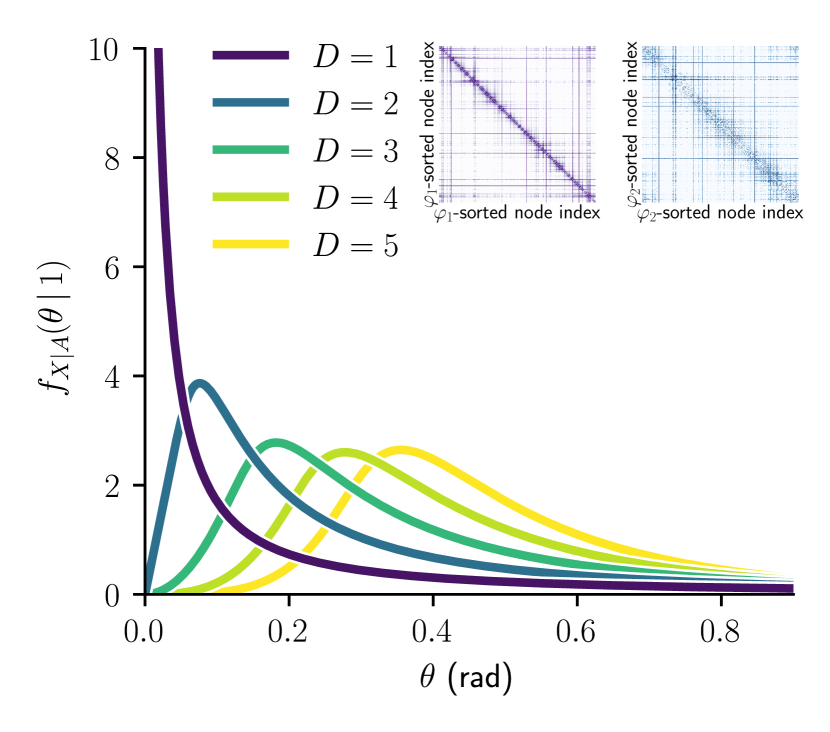
Figure 4: Probability density functions of angular distance between connected nodes in the $\mathbb{S}^{D}$ model given by Eq. (23), for $N=1000$ nodes, $\nicefrac{{\beta}}{{D}}=3.5$ and with a Pareto latent degree distribution with $\bar{\kappa}=10.0$ and exponent $\gamma=2.5$. Inset show examples of $\mathbb{S}^{D}$ connection probability matrices sampled with the same parameters, for $D=1$ (left) and $D=2$ (right). The node indices were sorted to satisfy $i<j$ when $\varphi_{D}(i)<\varphi_{D}(j)$, where $\varphi_{D}(i)$ denotes the coordinate $\varphi_{D}\in[0,2\pi)$ of the $i$-th node on the $D$-sphere.

Let us now zoom out of a specific pair of nodes and study the angular distance between connected nodes considering the entire latent degree distribution. To marginalize $\eta$ out of Eq. (17), one would need to compute

$$f_{X|A}(\theta\,|\,1)=\int_{\Omega_{Y}}f_{X|Y,A}(\theta\,|\,\eta,1)f_{Y|A}(\eta\,|\,1)\,\differential\eta,$$ (22)

where the integral is computed over all possible values of $\eta$. If we sample a graph from a $\mathbb{S}^{D}$ model, and then draw an edge uniformly at random, this is precisely the pdf of the angular distance between nodes creating that edge. Using Baye’s theorem, we can write

$$f_{Y|A}(\eta\,|\,1)=\frac{f_{A|Y}(1\,|\,\eta)f_{Y}(\eta)}{f_{A}(1)}.$$ (23)

Then, combining Eqs. (13)-(15) and (23) yields the following explicit form for Eq. (22):

$$f_{X|A}(\theta\,|\,1)=\frac{f_{X}(\theta)}{f_{A}(1)}\int_{\eta_{0}}^{\infty}\frac{f_{Y}(\eta)}{1+(\nicefrac{{\theta}}{{\eta}})^{\beta}}\,\differential\eta.$$ (24)

To further study the angular distance between connected nodes, the marginal pdf of $\eta$ has to be computed given the pdf of $\kappa$, which is done in Appendix A, along with the computation for $f_{A}(1)$.

Figure 4 illustrates the behavior of Eq. (24) for ${D\in\{1,2,3,4,5\}}$, with expected degrees that follow the same Pareto distribution in all dimensions. The differences between $D=1$ and $D>1$ found in the pairwise case are still notable when we consider the whole distribution. Those are the concentration of connected nodes at very small angular distances for $D=1$, the mode shifting towards higher angular distances with increasing dimension and the qualitative difference between the shape of distributions between $D=1$ and $D>1$. This effect of dimensionality, somewhat expected on its own, is to be interpreted in the light of other properties of higher-dimensional spaces studied in the following sections.

III.2 Number of nearest neighbors

Dimension affects angular closeness of nodes in hyperbolic graphs, but on a more elementary level it also impacts how many points can be closest to each other on $D$-spheres. If a finite number $n>2$ of points is spread on a circle, any given point will always have two, and only two, nearest neighbors. This, however, ceases to be true on higher-dimensional spheres, where the number of nearest neighbors then depends on the number of points $n$. To quantify this, let us define a characteristic neighborhood $\mathcal{B}(\phi_{n})\subset S^{D}(\hat{R})$ as an open ball (with respect to the standard great-circle distance) on the sphere, with angular radius $\phi_{n}$ of the ball chosen such that

$$\mathrm{Vol}(\mathcal{B}(\phi_{n}))=\frac{\mathrm{Vol}(S^{D}(\hat{R}))}{n}.$$ (25)

The volume refers to the $D$-dimensional measure of the $D$-sphere, i.e. the circumference of the circle, the surface area of the sphere, the volume of the $3$-sphere, and so on. The division of the space into areas of equal volume in Eq. (25) allows one to define the number of nearest neighbors $n_{\mathrm{nn}}$ as

$$n_{\mathrm{nn}}=\frac{\mathrm{Vol}(\mathcal{B}(3\phi_{n}))}{\mathrm{Vol}(\mathcal{B}(\phi_{n}))}-1.$$ (26)

The idea is to compute the volume of an open ball of radius ${3\phi_{n}}$ on $S^{D}(\hat{R})$ and assume that it contains ${1+n_{\mathrm{nn}}}$ points, a central one and its nearest neighbors. The definition of $n_{\mathrm{nn}}$ is an extension of $D=1$, where $\mathcal{B}(\phi_{n})$ is simply an arc of length $\nicefrac{{2\pi\hat{R}}}{{n}}$. In this simplest space, we trivially have

$$n_{\mathrm{nn}}=\frac{3\phi_{n}\hat{R}}{\phi_{n}\hat{R}}-1=2$$ (27)

for all ${n>2}$, in accordance with our previous intuition.

Furthermore, open balls on $S^{2}(\hat{R})$ are spherical caps of surface area ${2\pi\hat{R}^{2}[1-\cos\phi_{n}]}$. Using Eq. (25) to fix the value of $\phi_{n}$, it follows that for ${D=2}$,

$$n_{\mathrm{nn}}=\frac{n}{2}\quantity[1-\cos\quantity(3\acos\quantity(1-\nicefrac{{2}}{{n}}))]-1\\ =\frac{16}{n^{2}}-\frac{24}{n}+8\ ,$$ (28)

where we used the cosine triple angle formula. For general dimension $D$, $\mathcal{B}(\phi_{n})$ is a hyperspherical cap of volume

$$\mathrm{Vol}(\mathcal{B}(\phi_{n}))=\frac{2\pi^{\nicefrac{{D}}{{2}}}\hat{R}^{D}}{\Gamma(\nicefrac{{D}}{{2}})}\int_{0}^{\phi_{n}}\sin^{D-1}\theta\,d\theta.$$ (29)

It follows that

$$n_{\mathrm{nn}}=\frac{n\Gamma\quantity(\frac{D+1}{2})}{\sqrt{\pi}\Gamma\quantity(\frac{D}{2})}\int_{0}^{3\phi_{n}}\sin^{D-1}\theta\,d\theta-1,$$ (30)

where $\phi_{n}$ satisfies Eq. (25) using the volume of Eq. (29).

When $n\gg 1$, il follows that $\phi_{n}\ll 1$. Using the approximation $\sin x\approx x$ over the integration domains of Eqs. (29) and (30), we find the asymptotic number of nearest neighbors

$$n_{\mathrm{nn}}\overset{n\gg 1}{\approx}3^{D}-1.$$ (31)

In this regime, characteristic neighborhoods are equivalent to open balls in $\mathbb{R}^{D}$, since $S^{D}$ are manifolds, thus locally Euclidean by definition. Equation (31) can therefore be interpreted in the light of results from Draisma et al. (2012), where $3^{D}-1$ is the maximal number of lattice directions inside a connected set of $\mathbb{R}^{D}$. For $D\in\{1,2,3\}$, the value of Eq. (31) can be pictured quite intuitively in Euclidean space as shown in Fig. 5, hence justifying the apparently ad hoc definition of $n_{\mathrm{nn}}$. For instance, in an infinite square grid in $\mathbb{R}^{2}$, one square always has $8=3^{2}-1$ neighbors.

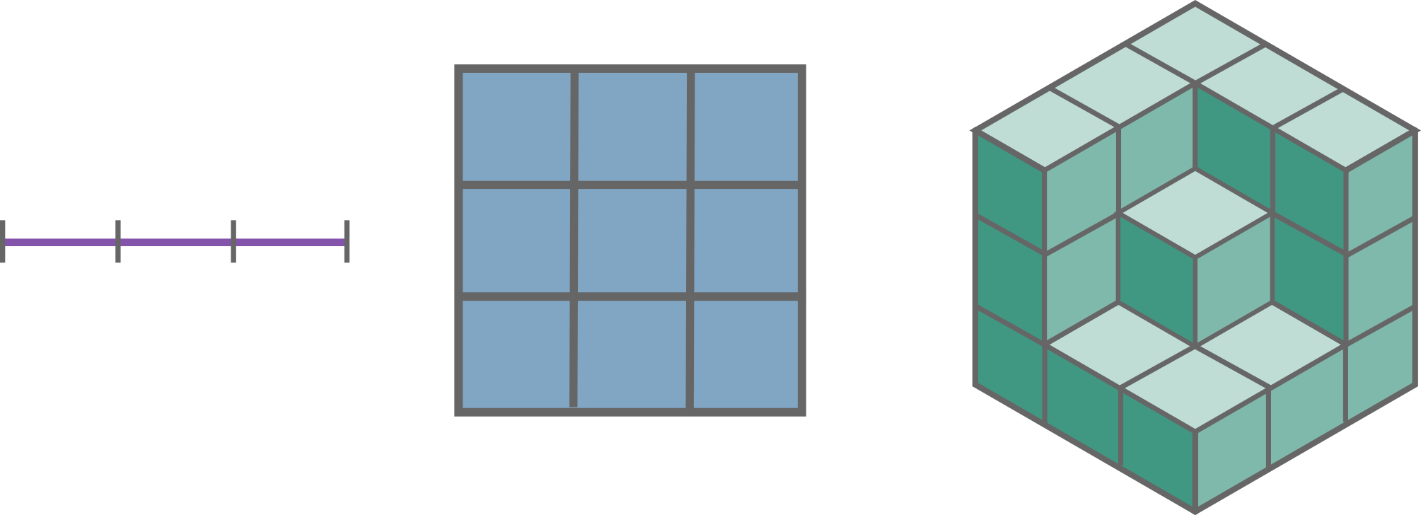
Figure 5: Neighboring line segments ($D=1$), squares ($D=2$) and cubes ($D=3$) in Euclidean space.

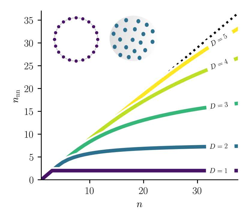
Figure 6: Number of nearest neighbors $n_{\mathrm{nn}}$ given by Eq. (26) for $D\in\{1,2,3,4,5\}$. The dotted line is at ${n-1}$, the maximal number of neighbors for $n$ points on $S^{D}$. The inset shows a circle and a sphere to exemplify neighboring points in $D=1$ and $D=2$.

As depicted in Fig. 6, $n_{\mathrm{nn}}$ is the same in any dimension when $n$ is low and only a few points are spread on $S^{D}$. But with higher dimensions, $n_{\mathrm{nn}}$ keeps on increasing up to higher asymptotic limits given by Eq. (31).

Now if, instead of counting points, $n$ were the number of angular communities within a hyperbolic network, either real embedded networked data or a random graph model, this geometrical property of $D$-spheres would limit the number of communities that could be connected. The following section frame more precisely how the two effects of dimensionality we just highlighted influence community modeling within $\mathbb{S}^{D}$ networks models.

IV Impacts on community structure

A community is a collection of nodes that are (typically) more densely connected together than to the rest of the network, which is captured in geometric networks by a fraction of nodes that are closer together in the space. In hyperbolic networks, community structure is modeled through angular aggregation of nodes on the spherical similarity space, thus creating soft communities Zuev et al. (2015). In real networks embedding on $\mathbb{S}^{1}$, nodes sharing qualitative attributes correlated with communities have been observed to form angular clusters. This was first observed in Boguñá et al. (2010) on the internet network, then in other types of data like economic and biological networks García-Pérez et al. (2016, 2019); Allard and Serrano (2020). On the other hand, methods for generating modules in random hyperbolic models have also used angular closeness, either through some variant of geometric preferential attachment mechanism Zuev et al. (2015); García-Pérez et al. (2018) or by direct sampling of clusters as angular coordinates Muscoloni and Cannistraci (2018).

Dimensionality has consequences on ways in which nodes can be nearby in $\mathbb{S}^{D}$, and how angular closeness is not as binding to connectivity when $D>1$. We proceed to show how the previous findings impact community structure modeling in hyperbolic networks for ultra-low dimensions $D\in\{1,2\}$. Numerical simulations of hyperbolic random graphs possessing community structure are at the core of the following section. Communities are generated as angular clusters and latent degrees are fixed subsequently. Once coordinates are well defined, we coarse-grain hyperbolic random graphs into block matrices that encode inter-community relations as simple weighted networks. Some global and local quantities are then measured on those block matrices to capture how communities can be related to each other in hyperbolic random graphs. This characterizes how community structure is impacted in $\mathbb{S}^{D}$ at the transition between $D=1$ and $D=2$.

IV.1 Generating communities in hyperbolic spaces

We consider the simplest possible case where all angular communities are of similar sizes and uniformly spread on the space, with latent degrees fixed subsequently to achieve a Pareto expected degree distribution in the random graph. This allows us to experiment with simple soft community structure—yet general—random graphs that possess all relevant properties of hyperbolic networks.

(a)

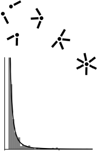
(b)

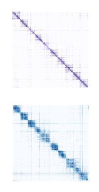
(c)

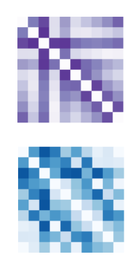
(d)

Figure 7: Example of sampling hyperbolic random graphs with angular community structure in $\mathbb{S}^{1}$ and $\mathbb{S}^{2}$. Angular coordinates (a) are used to optimize latent degrees such that a given expected degree distribution (b) is achieved. The random graphs are then fully specified by Eq. (5), which is illustrated in (c) matrices of connection probabilities between all nodes, ordered with polar coordinates within each community. Those are then coarse-grained into block matrices (d) using Eq. (32) to study inter-community interactions in hyperbolic spaces.

Let $n$ be the number of angular communities we wish to generate. Angular coordinates for each node are first sampled such that $n$ clusters are distributed homogeneously on the space, as shown in Fig. 7(a). The disparity of nodes within each angular cluster is tuned via a parameter $\sigma\in[0,1]$ comparable to the standard variation of normal distributions. When $\sigma=0$, all nodes of a cluster have the same angular coordinate, whereas when $\sigma=1$, sampling is roughly equivalent from sampling points uniformly on $S^{D}$. This procedure is similar to sampling Gaussian mixtures on the circle of Ref. Muscoloni and Cannistraci (2018), more details are given in Appendix B and the code is freely available online Désy (2022).

Once angular coordinates are fixed, latent degrees are optimized to obtain a Pareto expected degree distribution using the scheme of Ref. (García-Pérez et al., 2018, Sec. 2.1.2), with a tolerance of 0.2. We model independently the angular coordinates and the latent degrees, which is equivalent to assuming that the similarity space giving rise to some community structure is decoupled from the degrees of nodes within the graph. It follows from this assumption that the degree distribution within each angular cluster is drawn independently from the same distribution. With such angular coordinates and latent degrees, the hyperbolic random graph is fully defined by the connection probabilities of Eq. (5). Each node ${i=1,\ldots,N}$ has an additional community label $c_{i}=1,\ldots,n$ describing its membership to one of the angular clusters, which is redefined as the closest centroid. It follows that all communities are of similar size, albeit not identical, and that there is no overlap between communities, as exemplified in Fig. 8(b).

To study community structure, each random graph is mapped to a weighted graph of inter-community edges probabilities. Consider the $n\times n$ matrix

$$B_{uv}=\frac{1}{m}\sum_{i=1}^{N}\sum_{j=1}^{N}p_{ij}\delta(c_{i},u)\delta(c_{j},v)(1-\delta(c_{i},c_{j})),$$ (32)

where $m:=\sum_{i<j}p_{ij}(1-\delta(c_{i},c_{j}))$ is the sum of probabilities associated with inter-communities edges, which can be interpreted as the total expected number of edges between distinct communities. Matrix $B$’s elements are normalized sums of edge probabilities between two communities, with diagonal set to zero. Thus, $B$ can be thought of as a weighted graph describing how distinct communities interact with each other. It is normalized with the total expected number of inter-community edges such that $B_{uv}$ quantifies the probability of finding an edge between the corresponding pair of communities $u$ and $v$. The complete procedure to sample a given random graph to obtain a block matrix $B$ is illustrated in Fig. 7.

IV.2 Global assessment of angular dependency

Anecdotally, blocks near the diagonal within matrices of Fig. 7(d) suggest that community structure in $\mathbb{S}^{1}$ is impacted differently than in $\mathbb{S}^{2}$. Indeed, similarly-generated hyperbolic random graphs in $\mathbb{S}^{2}$ look more permissive with regards to how community blocks can be related to one another. To quantify these observations, we use the stable rank and the Shannon entropy of matrices $B$. Both quantities are global measures of matrix structure, related in a complementary way to how diagonal versus uniform a matrix can be.

IV.2.1 Stable rank

The rank of a matrix is a global measure intimately related to dimensionality. In its formal definition, the rank is the maximum number of linearly independent columns or rows of a matrix, thus counting the dimension of the vector space it generates Horn and Johnson (2013). When working with noisy or random matrices, it is more convenient to use the stable rank, also called numerical rank or effective rank, and defined as

$$\mathrm{srank}(B)=\frac{1}{s_{1}^{2}}\sum_{i=1}^{n}s_{i}^{2},$$ (33)

where $s_{i},\,i=1,\ldots,n$ are the singular values of $B$ in non-increasing order Rudelson and Vershynin (2007); Vershynin (2018). The stable rank is always bounded above by the usual rank and is maximal for the identity matrix, diagonal matrices with non-zero diagonal elements, or Toeplitz matrices of the form

$$B=\begin{pmatrix}b&c&0&\cdots\\ a&b&c&\ddots\\ 0&a&b&\ddots\\ \vdots&\ddots&\ddots&\ddots\end{pmatrix},$$

which makes it useful for quantifying to which extent matrix entries are concentrated near the diagonal. Moreover, the stable rank is invariant under any similarity transformation $B\mapsto PBP^{\top}$, where $P$ is a permutation matrix, thus ensuring that the value of $\mathrm{srank}(B)$ is independent of the node labelling in the graph corresponding to $B$.

Since we compare different number of communities, hence block matrices of different order, we choose to work with the srank-to-dimension ratio,

$$r(B)=\frac{\mathrm{srank}(B)}{n},$$ (34)

a version of the stable rank normalized by its maximal possible value Thibeault et al. (2022). It follows that $r(B)=1$ for a matrix of maximal rank, for instance a diagonal matrix, and $r(B)=0$ for a null matrix. In between those extremes, $r(B)$ captures to which extent the entries of $B$ could be permuted to yield a diagonal matrix. In the context of community block matrices, this allows us to evaluate the complexity of connection patterns between communities.

In Fig. 8(a), we show that for various number of communities $n$ and angular dispersion of nodes $\sigma$, $r$ is always higher on $\mathbb{S}^{1}$ than $\mathbb{S}^{2}$. Higher srank of the $D=1$ block matrices quantifies how the inter-communities edge weights are more strictly bounded near the diagonal compared to $D=2$. This difference is less notable when angular communities are few ($n=5$) and highly concentrated ($\sigma\in[0.1,0.2]$), since then the additional dimension has the least impact on the neighborhood of nodes because respectively, they are mostly connected within one community. In other parameter regimes, the difference between $\mathbb{S}^{1}$ and $\mathbb{S}^{2}$ experimentally expresses the strong angular dependence of connectivity patterns explained in §III.1, when specifically applied to community structure.

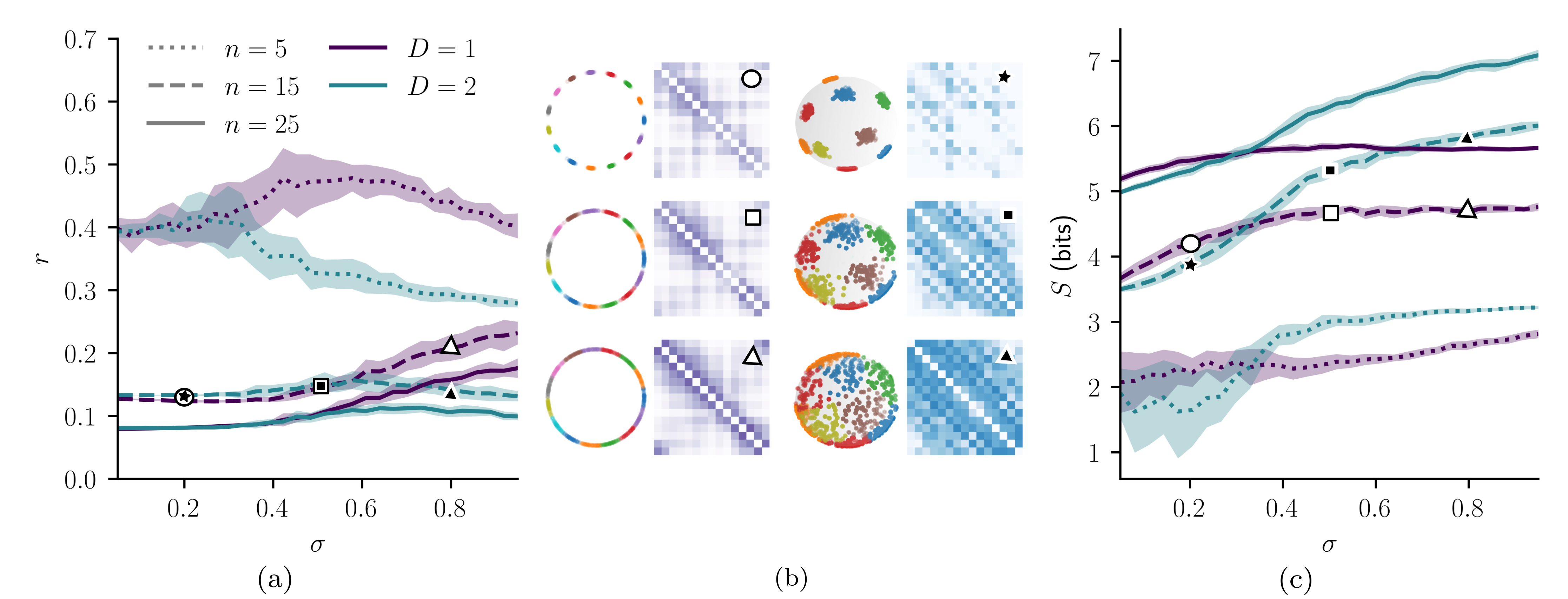
Figure 8: (a) Stable rank to dimension ratio and (c) Shannon entropy of community block matrices in $\mathbb{S}^{1}$ and $\mathbb{S}^{2}$, when increasing the angular dispersion of nodes. The center panel (b) illustrates examples of angular coordinates and block matrices with $\sigma\in\{0.2,0.5,0.8\}$ for ${D=1}$ (purple matrices) and ${D=2}$ (blue matrices) with corresponding values of stable rank and entropy indicated with symbols on (a) and (c). All the graphs have $\nicefrac{{\beta}}{{D}}=3.5$ and a Pareto expected degree distribution with average degree of 4.0 and $\gamma=2.5$.

IV.2.2 Shannon entropy

Shannon entropy Shannon (1948) quantifies to which extent the probability mass function of a discrete random variable is uniform. It is often intuitively described as a measure of how uncertain the outcome of a random event is. As currently defined, matrices $B$ describe the probability mass function of a single edge between two communities. It follows that the Shannon entropy of $B$ matrices,

$$S(B)=-\sum_{u<v}B_{uv}\log_{2}(B_{uv}),$$ (35)

quantifies how uniform block matrices are, in bits. This entropy is zero if only one entry of $B$ has value 1, depicting a maximally non-uniform community structure. Conversely, $S(B)$ reaches its maximal value, $\log_{2}(\nicefrac{{n(n-1)}}{{2}})$, if the matrix $B$ is entirely uniform with $B_{uv}=\nicefrac{{2}}{{n(n-1)}}$ for all $\nicefrac{{n(n-1)}}{{2}}$ possible community unordered pairs $(u,v)$.

Figure 8(c) shows that as nodes angular dispersion increases, block matrices in $\mathbb{S}^{2}$ have an increasing entropy. This quantifies how block matrices in $D=2$ are more and more uniform as nodes scatter across the space. Conversely, block matrices in $\mathbb{S}^{1}$ uphold the same tridiagonal structure, which is reflected in the stagnation of the entropy. Again, the difference in behavior is minimal for $n=5$, but for $n\in\{15,25\}$ it is not. A higher Shannon entropy of block matrices in $D=2$, or their uniformity, means that any given community is likely to be connected to many other communities. This effect is quantified more precisely in the following section.

IV.3 Local count of neighboring communities

We also evaluate community degrees as a hyperbolic random graph equivalent to the number of nearest neighbors $n_{\mathrm{nn}}$ of Sec. III.2. Community degrees are computed as rows sum of a binary version of the community block matrix $B$. We binarize matrix $B$ through the following mapping

$$C_{uv}=\begin{cases}1&\text{ if }B_{uv}>\nicefrac{{1}}{{m}},\\ 0&\hfil\text{ otherwise},\end{cases}$$ (36)

where $m$ is the sum of probabilities associated with inter-communities edges, as defined below Eq. (32). If the expected value of the number of edges between two communities is greater or equal than 1, that is to say we expect at least one edge between communities $u$ and $v$ on average in the random graph, then the two communities are related. This is a very liberal way to binarize $B$; other thresholds or methods could have been used. In Appendix C, we show that our numerical results for comparison of $\mathbb{S}^{1}$ and $\mathbb{S}^{2}$ are valid for other binarization procedures.

The degree of community $u$ is then defined as

$$k_{u}=\sum_{v=1}^{n}C_{uv},$$ (37)

which quantifies the number of other communities $u$ is related to. We then define the average community degree as

$$\expectationvalue{k}=\frac{1}{n}\sum_{u=1}^{n}k_{u}.$$ (38)

In Fig. 9, we show the average community degree for hyperbolic random graphs with angular communities sampled according to the scheme described in Sec. IV.1. As expected, with only $n=5$ angular communities, the dimension has very little impact and both models reach a value of nodes dispersion $\sigma$ where all communities are related to $n-1$ others. Yet, when more angular clusters are considered, $\expectationvalue{k}$ in $\mathbb{S}^{1}$ barely increases,whereas in $\mathbb{S}^{2}$ communities keep on relating to more others as nodes get more dispersed on the sphere.

An upper bound on community degree in $D=1$ is suggested by the purple curves of Fig. 9, although this is not the same phenomenon as the strict limits of Fig. 6. In §III.2, the hyperbolic connection probability was not considered and the meaning of a neighborhood was purely geometric, with $n_{\mathrm{nn}}$ varying with $n$. Here, we vary the angular dispersion on nodes for a given number of communities $n$. Yet in $\mathbb{S}^{1}$, the circular boundary still poses an upper limit to how many communities can be related together. As opposed to $n_{\mathrm{nn}}=2$ in $D=1$, the numerical upper bound of Fig. 9 is more than two other neighboring communities, thanks to this very permissive definition of community degree and to high degree nodes (having small radius in the hyperbolic representation) allowing for long angular range connections between communities.

This is yet another way to assess that in $\mathbb{S}^{1}$, most of the inter-community edges are concentrated to fewer nearest neighbors than in $D=2$, as exemplified in matrices of Fig. 8(b).

Figure 9: Average community degree $\expectationvalue{k}$ of hyperbolic random graphs with angular communities sampled in $\mathbb{S}^{1}$ and $\mathbb{S}^{2}$. All the graphs have $\nicefrac{{\beta}}{{D}}=3.5$ and a Pareto expected degree distribution with average degree of 4.0 and $\gamma=2.5$.

V Summary and future work

Recent developments in hyperbolic network geometry have challenged the common belief that only one underlying similarity dimension was enough to realistically capture the structure of real complex network Almagro et al. (2022). Although the impact of dimension on local properties like the degree distribution can be balanced by rescaling the abruptness of the connection probability through $\beta$ Yang and Rideout (2020); Kovács et al. (2022); Budel et al. (2023), as soon as one zoom out to mesoscopic properties like clustering or short cycles, non-trivial effects of dimension arise García-Pérez et al. (2018); Kovács et al. (2022); Almagro et al. (2022). Our work adds to this line of research by highlighting the interplay between dimension and community structure. We found that tighter angular bounds for connections in the $\mathbb{S}^{1}$ model unrealistically restricts the community structures that can be generated on hyperbolic random graphs. Yet, dimensionality can improve current modeling of community structure in the hyperbolic framework, which has already proven successful at capturing so many other important properties all at once Boguñá et al. (2020, 2021). We found that only one additional dimension expands the inter-community connection possibilities in a way that renders more realistic modular networks modeling in hyperbolic spaces.

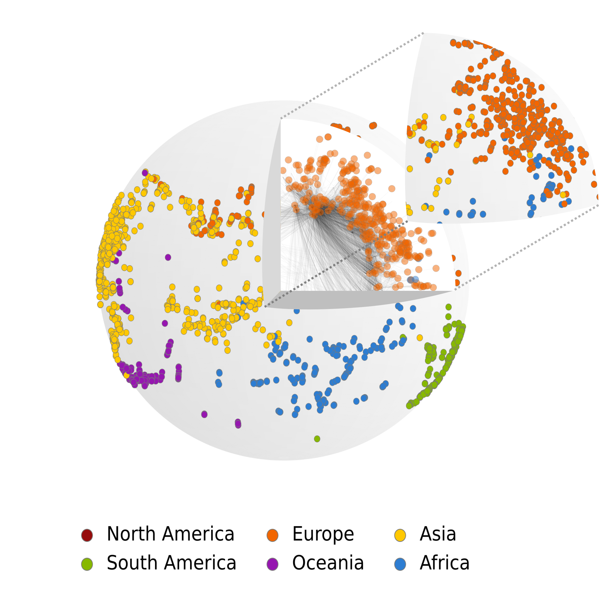
Figure 10: A schematic representation of the airports network from Fig. 1 embedded in $\mathbb{S}^{2}/\mathbb{H}^{3}$. Angular coordinates of nodes projected on the surface are estimated using the algorithm from Ref. Muscoloni et al. (2017). North American airports are hidden behind the sphere, see animation provided as Supplementary Material for a complete portrayal of nodes’ position on $\mathbb{S}^{2}$. Note that algorithm used here is based on machine learning heuristics and therefore does not maximizes the likelihood that the $\mathbb{S}^{2}/\mathbb{H}^{3}$ model presented in Sec. II generated the topology of the airports network as would standard algorithms like Mercator do García-Pérez et al. (2019). The inferred angular positions are therefore used here simply to illustrate the effect dimension has on the spatial distribution of communities.

In the first part of this paper, we have shown that realized edges in hyperbolic random graphs are mostly near zero angular distance in $D=1$, whereas it is not the case in greater dimension. This is quantified through the angular distance distribution between connected nodes given by Eq. (17), which has a mode that gets further away from $0$ as $D$ increases. Our main result is the sharp qualitative difference between the $D=1$ and $D>1$ cases, which is also prominent when the angular distance distribution is averaged over all nodes’ latent degrees. It follows that in $D>1$, connection patterns between individual nodes are less restricted by their angular proximity. Besides, the number of nearest neighbors for points on spherical manifolds is also an increasing function of the dimension. Thus, the number of nearest angular neighboring clusters of nodes, or soft communities in hyperbolic random graphs, varies with $D$, which reflects on community structure modeling.

To assess these effects, in the second part of this paper, we experimented numerically with hyperbolic random graphs in which nodes’ angular coordinates were grouped in soft communities in $D=1$ and $D=2$. By averaging the individual connection probabilities into the probabilities to find an edge between two distinct communities, we obtained block matrices describing inter-community relationships. The structure of these were studied across different values of angular dispersion of nodes to highlight differences arising from adding only one similarity dimension. Indeed, block matrices were more bounded to a diagonal shape by angular closeness in $D=1$, as quantified by their stable rank, and more uniform in $D=2$, as quantified by their Shannon entropy. The idea of having more uniform inter-community block matrices refers to the fact that in $D>1$, any given community can be related to more other communities, as also quantified by the average community degree. Akin to the number of nearest neighbors for points, the average community degree was higher in $D=2$, especially as soft communities were more dispersed angularly.

In $D=1$, mechanisms underlying soft-community formation and modeling in $\mathbb{S}^{1}$ and $\mathbb{H}^{2}$ Zuev et al. (2015); García-Pérez et al. (2018); Muscoloni and Cannistraci (2019) and the inherent modularity of hyperbolic random graphs Kovács and Palla (2021); Chellig et al. (2021) have been studied. However, we have argued here that hyperbolic network models of varying dimensions are quite distinct when it comes to their potential to model community structure, in particular between $D=1$ and $D>1$. Community structures as simple as a triplet of strongly interacting communities are poorly captured in $D=1$, as exemplified by the African, Asian, and European airports in Fig. 1, whereas the same overlapping communities become disentangled in $D=2$, as shown in Fig. 10 and in the animation provided as Supplementary Material. The advantage of $D>1$ over $D=1$ for representing community network data was also reported in Ref. Muscoloni and Cannistraci (2019). Since most real-world networks possess some sort of nodes’ aggregates, this suggests that the recently discovered higher underlying hyperbolic dimension for most real-world networks by Ref. Almagro et al. (2022) could be related to their mesoscale structure, although dimension detection is beyond the scope of our paper and should be explored in future work.

Increasing the dimensionality of the underlying hyperbolic spaces might also help to improve the likelihood maximization procedure that is used for inferring hyperbolic coordinates for networked data. As observed for three different embedding algorithms Papadopoulos et al. (2015a); Muscoloni et al. (2017); García-Pérez et al. (2018), inferring angular coordinates can be considered the hardest part of the hyperbolic embedding procedure. The use of common neighbors has been considered in Ref. Papadopoulos et al. (2015b) to solve this issue. We have shown that the number of nearest angular neighbors increases with dimension, as does the diversity of community structures that can be generated. Hence our conjecture that higher, albeit still ultra-low, dimensional hyperbolic spaces would more realistically capture the structure of networks and be inferred without such angular degeneracy.

Another way to see this is with a simple thought experiment. Let us assume there exist some networks whose topology is naturally reflected by a higher underlying hyperbolic dimension. For instance, one could think of a randomly generated network in $\mathbb{H}^{D+1}$ with $D>1$, or a real network like the internet which, according to Ref. (Almagro et al., 2022, Fig. 5) could have a dimension as high as $D=7$. If such a network were to be embedded in $\mathbb{H}^{2}$, the geometric neighborhoods of nodes (which node is close to which others) could not be respected, since as we show in Sec. III.B. the number of nearest angular neighbors varies with dimension. Therefore, any lower-dimensional embedding will have to accommodate by positioning some nodes closer than they should and vice versa, which would reflect on tasks like link prediction, for instance. We wish we could carry out this experiment, but current embedding algorithms are yet to be generalized to more dimensions García-Pérez et al. (2019), or have only been used on relatively small networks Muscoloni et al. (2017); Muscoloni and Cannistraci (2019) in $D=2$.

Knowledge about community structure has already been shown to impact performance of very diverse network tasks, from hyperbolic embedding coordinate inference Faqeeh et al. (2018); Wang et al. (2016a, b) to dimension reduction Jiang et al. (2018); Thibeault et al. (2020); Vegué et al. (2022), efficient information communication Lynn et al. (2020) and resilience Dong et al. (2018). A natural way to push our work will then be to study how this coupling between community structure and the underlying dimension of hyperbolic networks affects tasks which have already been shown to perform better in the framework of hyperbolic network geometry. In particular, greedy routing of information propagation has been one of the first and most interesting assets of hyperbolic geometry Boguñá and Krioukov (2009); Allard and Serrano (2020), which should be studied in higher dimensions while explicitly considering community structure.

Another intriguing direction of research would be to use hierarchical network generation mechanisms like geometric branching growth Zheng et al. (2019) in higher dimensions. Such a procedure generates a hyperbolic network through subdivision of a small initial network into finer and finer descendants, a statistical inverse of geometric renormalization García-Pérez et al. (2018). By placing the initial seed network into higher-dimensional spaces, one could compare hierarchical community structure in different dimensions. This would be akin to our numerical study but in a more complex setting where the nodes angular coordinates follow a hierarchical structure.

Code availability

The code used to produce all figures is written in the Python programming language and is available on Zenodo and Github Désy (2022).

Author contribution

B.D., P.D and A.A designed the research, as well as analyzed and interpreted the results. B.D. and A.A. wrote the codes for the numerical experiments. B.D. performed the research and wrote the manuscript. All authors read, commented, edited, and approved the final version of the manuscript.

Appendix A Explicit computations for angular densities

A.1 Modes of angular distance between connected node pairs

Taking the first derivative of Eq. (17) with respect to $\theta$ and setting it to zero yields

$$\frac{(D-1)\sin^{D-2}\theta^{*}\cos\theta^{*}}{1+(\nicefrac{{\theta^{*}}}{{\eta}})^{\beta}}=\frac{\sin^{D-1}\theta^{*}}{\quantity[1+(\nicefrac{{\theta^{*}}}{{\eta}})^{\beta}]^{2}}\frac{\beta(\nicefrac{{\theta^{*}}}{{\eta}})^{\beta}}{\theta^{*}},$$ (39)

where $\theta^{*}$ can be a minimum, a maximum or an inflexion point. We separate two cases:

1. If $\theta^{*}\in(0,\pi)$, Eq. (39) can be simplified to Eq. (19).

2. We proceed to show that $\theta^{*}=0$ iff $D=1$ in the regime $\beta>D,\,\eta>0$. First, if $D=1$, Eq. (39) reduces to

   $$0=\frac{\beta(\nicefrac{{\theta^{*}}}{{\eta}})^{\beta}}{\theta^{*}\quantity[1+(\nicefrac{{\theta^{*}}}{{\eta}})^{\beta}]^{2}},$$ (40)

   which is verified only for $\theta^{*}=0$. Conversely, setting $\theta^{*}=0$ in Eq. (39) trivially yields $D=1$.

A.2 Probability density function for $\eta$

Since $\eta$ is a scalar function of $\kappa,\kappa^{\prime}$, the pdf for $Y$ can be computed as follows.

$$f_{Y}(\eta)=\int_{\Omega_{K}}\int_{\Omega_{K}}\rho_{K}(\kappa)\rho_{K}(\kappa^{\prime})\delta(g(\kappa^{\prime}))\,\differential\kappa\,\differential\kappa^{\prime}$$ (41)

with $g(\kappa^{\prime}):=\eta-\nicefrac{{(\mu\kappa\kappa^{\prime})^{\nicefrac{{1}}{{D}}}}}{{R}}$ and $\delta$ the Dirac delta function. By definition of composition with the Dirac delta function under the integral,

$$\delta(g(\kappa^{\prime}))=\frac{\delta(\kappa^{\prime}-\kappa^{\prime}_{*})}{|g^{\prime}(\kappa^{\prime}_{*})|},$$ (42)

with ${\kappa^{\prime}_{*}=\nicefrac{{(\eta R)^{D}}}{{\mu\kappa}}}$, the unique root of $g$. Hence

$$\derivative{g}{\kappa^{\prime}}\evaluated{}_{\kappa^{\prime}=\kappa^{\prime}_{*}}=\frac{\mu\kappa\eta^{(1-D)}}{DR^{D}}>0,$$ (43)

and it follows that

$$\delta(g(\kappa^{\prime}))=\frac{\delta(\kappa^{\prime}-\nicefrac{{(\eta R)^{D}}}{{\mu\kappa}})}{\mu\kappa\eta^{(1-D)}}DR^{D}.$$ (44)

Eq. (41) can thus be computed as

$$f_{Y}(\eta)=\frac{DR^{D}}{\mu\eta^{1-D}}\int_{0}^{\infty}\rho_{\kappa}(\kappa)\rho_{\kappa}(\nicefrac{{(\eta R)^{D}}}{{\mu\kappa}})\frac{d\kappa}{\kappa}.$$ (45)

For any distribution of $\kappa$ with a non-zero lower bound $\kappa_{0}$,

$$\frac{(\eta R)^{D}}{\mu\kappa}<\kappa_{0}\quad\iff\quad\frac{(\eta R)^{D}}{\mu\kappa_{0}}<\kappa,$$ (46)

which means that the integrand in Eq. (45) is null in the regime of Eq. (46). We finally have

$$f_{Y}(\eta)=\frac{DR^{D}}{\mu\eta^{1-D}}\int_{\kappa_{0}}^{\nicefrac{{(\eta R)^{D}}}{{\mu\kappa_{0}}}}\rho_{\kappa}(\kappa)\rho_{\kappa}(\nicefrac{{(\eta R)^{D}}}{{\mu\kappa}})\frac{d\kappa}{\kappa}.$$ (47)

This pdf can be computed exactly for $\kappa$ drawn from a Pareto distribution with parameter $\gamma$. Let

$$\rho_{\kappa}(\kappa)=(\gamma-1)\kappa_{0}^{\gamma-1}\kappa^{-\gamma},$$ (48)

then computation of the integral in Eq. (47) gives

$$f_{Y}^{\mathrm{Pareto}}(\eta)=\frac{D(\gamma-1)^{2}\kappa_{0}^{2(\gamma-1)}\mu^{\gamma-1}}{R^{D(\gamma-1)}\eta^{D(\gamma-1)+1}}\log\quantity[\frac{(\eta R)^{D}}{\mu\kappa_{0}^{2}}].$$ (49)

A.3 Marginalized connection probability

Since the connection probability of hyperbolic random graphs (Eq. (5)) depends on $\theta$ and $\eta$, one would need to know the pdf for $\theta$ and the pdf for $\eta$ to compute the marginalized connection probability that appears in the normalization of Eq. (24).

$$f_{A}(1)=\int_{\Omega_{Y}}\int_{\Omega_{X}}f_{X,Y,A}(\theta,\eta,1)\,\differential\theta\,\differential\eta.$$ (50)

Given $\Omega_{X}=[0,\pi]$, $\Omega_{Y}=[\eta_{0},\infty)$ and Eq. (14),

$$f_{A}(1) =\int_{\eta_{0}}^{\infty}\int_{0}^{\pi}\frac{\sin^{D-1}\theta\,f_{Y}(\eta)}{I_{D}[1+(\nicefrac{{\theta}}{{\eta}})^{\beta}]}\,\differential\theta\,\differential\eta$$ (51)

$$=\frac{1}{I_{D}}\int_{\eta_{0}}^{\infty}\quantity[\int_{0}^{\pi}\frac{\sin^{D-1}\theta}{1+(\nicefrac{{\theta}}{{\eta}})^{\beta}}\,\differential\theta]f_{Y}(\eta)\,\differential\eta$$ (52)

$$=\frac{\sqrt{\pi}\Gamma(\nicefrac{{D}}{{2}})}{\Gamma(\nicefrac{{D+1}}{{2}})}\int_{\eta_{0}}^{\infty}\mathcal{Z}(\eta)f_{Y}(\eta)\,\differential\eta,$$ (53)

where the angular distance distribution of Eq. (11) and the definition of Eq. (18) have been used.

Appendix B Sampling methods

To sample clusters of angular coordinates for hyperbolic random graphs in $D=2$, we first distribute the modes of all $n$ clusters evenly using the Fibonacci lattice algorithm González (2009). Then, coordinates of nodes within each cluster are sampled from a three-dimensional normal distribution in $\mathbb{R}^{3}$ centered around its mode, and then projected on the unit sphere. Lastly, the community to which each node belongs is defined as the one of the closest mode, or as the closest centroid. This allows us to obtain a given number $n$ of evenly distributed clusters of angular coordinates for the nodes.

Appendix C Other thresholding methods for block matrices

Here we validate that results about community degree of Sec. IV.3 are robust to other binarization methods. In Fig. 11, we show the community degree $\expectationvalue{k}$ measured on the same matrices as the ones used for Fig. 9, but using a higher threshold (left) and the disparity filter of Ref. Serrano et al. (2009) (right) to transform the inter-community edges probability matrix $B$ to a binary matrix. Both plots show that community degree in $\mathbb{S}^{2}$ increases to higher values than in $\mathbb{S}^{1}$. The disparity filter penalizes locally homogeneous edge weights, which explains why the blue curves on the right panel do not increase as much as in Fig. 9, since then the inter-community edge probability becomes more and more homogeneous on the neighboring angular clusters.

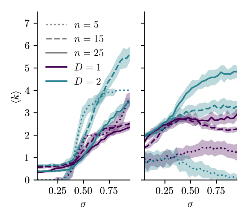
Figure 11: Community degree $\expectationvalue{k}$ with alternative binarization methods. On the left, Eq.(37) is used with a higher threshold of $10/m$ and on the right, the disparity filter of Ref. Serrano et al. (2009) is applied with $\alpha=0.2$.

References

- Boguñá et al. (2010) Marián Boguñá, Fragkiskos Papadopoulos, and Dmitri Krioukov, “Sustaining the Internet with hyperbolic mapping,” Nature Communications 1, 1–8 (2010).
- Allard and Serrano (2020) Antoine Allard and M. Ángeles Serrano, “Navigable maps of structural brain networks across species,” PLoS computational biology 16, e1007584 (2020).
- Boguñá et al. (2021) Marián Boguñá, Ivan Bonamassa, Manlio De Domenico, Shlomo Havlin, Dmitri Krioukov, and M. Ángeles Serrano, “Network geometry,” Nature Reviews Physics 3, 114–135 (2021).
- Boguñá et al. (2020) Marián Boguñá, Dmitri Krioukov, Pedro Almagro, and M. Ángeles Serrano, “Small worlds and clustering in spatial networks,” Physical Review Research 2, 023040 (2020).
- Papadopoulos et al. (2012) Fragkiskos Papadopoulos, Maksim Kitsak, M. Ángeles Serrano, Marián Boguñá, and Dmitri Krioukov, “Popularity versus similarity in growing networks,” Nature 489, 537–540 (2012).
- García-Pérez et al. (2016) Guillermo García-Pérez, Marián Boguñá, Antoine Allard, and M. Ángeles Serrano, “The hidden hyperbolic geometry of international trade: World trade atlas 1870–2013,” Scientific Reports 6, 33441 (2016).
- Zheng et al. (2019) Muhua Zheng, Guillermo García-Pérez, Marián Boguñá, and M. Ángeles Serrano, “Scaling up real networks by geometric branching growth,” Proceedings of the National Academy of Sciences 118, e2018994118 (2019).
- Allard et al. (2017) Antoine Allard, M. Ángeles Serrano, Guillermo García-Pérez, and Marián Boguñá, “The geometric nature of weights in real complex networks,” Nature Communications 8, 14103 (2017).
- Krioukov et al. (2012) Dmitri Krioukov, Maksim Kitsak, Robert S. Sinkovits, David Rideout, David Meyer, and Marián Boguñá, “Network cosmology,” Scientific Reports 2, 793 (2012).
- Kitsak et al. (2017) Maksim Kitsak, Fragkiskos Papadopoulos, and Dmitri Krioukov, “Latent geometry of bipartite networks,” Physical Review E 95, 032309 (2017).
- Kleineberg et al. (2016) Kaj-Kolja Kleineberg, Marián Boguñá, M. Ángeles Serrano, and Fragkiskos Papadopoulos, “Hidden geometric correlations in real multiplex networks,” Nature Physics 12, 1076–1081 (2016).
- Kleineberg et al. (2017) Kaj-Kolja Kleineberg, Lubos Buzna, Fragkiskos Papadopoulos, Marián Boguñá, and M. Ángeles Serrano, “Geometric correlations mitigate the extreme vulnerability of multiplex networks against targeted attacks,” Physical Review Letters 118, 218301 (2017).
- García-Pérez et al. (2018) Guillermo García-Pérez, M. Ángeles Serrano, and Marián Boguñá, “Soft Communities in Similarity Space,” Journal of Statistical Physics 173, 775–782 (2018).
- Zuev et al. (2015) Konstantin Zuev, Marián Boguñá, Ginestra Bianconi, and Dmitri Krioukov, “Emergence of soft communities from geometric preferential attachment,” Scientific Reports 5, 9421 (2015).
- Muscoloni and Cannistraci (2018) Alessandro Muscoloni and Carlo Vittorio Cannistraci, “A nonuniform popularity-similarity optimization (nPSO) model to efficiently generate realistic complex networks with communities,” New Journal of Physics 20, 052002 (2018).
- Yang and Rideout (2020) Weihua Yang and David Rideout, “High dimensional hyperbolic geometry of complex networks,” Mathematics 8, 1861 (2020).
- Almagro et al. (2022) Pedro Almagro, Marián Boguñá, and M. Ángeles Serrano, “Detecting the ultra low dimensionality of real networks,” Nature Communications 13, 60–96 (2022).
- Kovács et al. (2022) Bianka Kovács, Sámuel G Balogh, and Gergely Palla, “Generalised popularity-similarity optimisation model for growing hyperbolic networks beyond two dimensions,” Scientific Reports 12, 968 (2022).
- Budel et al. (2023) Gabriel Budel, Maksim Kitsak, Rodrigo Aldecoa, Konstantin Zuev, and Dmitri Krioukov, “Random hyperbolic graphs in dimensions,” arXiv.2010.12303 , (2023).
- Gu et al. (2021) Weiwei Gu, Aditya Tandon, Yong-Yeol Ahn, and Filippo Radicchi, “Principled approach to the selection of the embedding dimension of networks,” Nature Communications 12, 3772 (2021).
- García-Pérez et al. (2018) Guillermo García-Pérez, Marián Boguñá, and M. Ángeles Serrano, “Multiscale unfolding of real networks by geometric renormalization,” Nature Physics 14, 583–589 (2018).
- Girvan and Newman (2002) M. Girvan and M. E. J. Newman, “Community structure in social and biological networks,” Proceedings of the National Academy of Sciences 99, 7821–7826 (2002).
- Cherifi et al. (2019) Hocine Cherifi, Gergely Palla, Boleslaw K. Szymanski, and Xiaoyan Lu, “On community structure in complex networks: challenges and opportunities,” Applied Network Science 4, 117 (2019).
- Milo et al. (2002) R. Milo, S. Shen-Orr, S. Itzkovitz, N. Kashtan, D. Chklovskii, and U. Alon, “Network motifs: Simple building blocks of complex networks,” Science 298, 824–827 (2002).
- Fortunato and Hric (2016) Santo Fortunato and Darko Hric, “Community detection in networks: A user guide,” Physics Reports 659, 1–44 (2016).
- Fortunato and Newman (2022) Santo Fortunato and Mark E. J. Newman, “20 years of network community detection,” Nat. Phys. 18, 848–850 (2022).
- Betzel et al. (2017) Richard F. Betzel, John D. Medaglia, Lia Papadopoulos, Graham L. Baum, Ruben Gur, Raquel Gur, David Roalf, Theodore D. Satterthwaite, and Danielle S. Bassett, “The modular organization of human anatomical brain networks: Accounting for the cost of wiring,” Network Neuroscience 1, 42–68 (2017).
- Betzel et al. (2019) Richard F. Betzel, Maxwell A. Bertolero, Evan M. Gordon, Caterina Gratton, Nico U.F. Dosenbach, and Danielle S. Bassett, “The community structure of functional brain networks exhibits scale-specific patterns of inter- and intra-subject variability,” NeuroImage 202, 115990 (2019).
- García-Pérez et al. (2019) Guillermo García-Pérez, Antoine Allard, M. Ángeles Serrano, and Marián Boguñá, “Mercator: uncovering faithful hyperbolic embeddings of complex networks,” New Journal of Physics 21, 123033 (2019).
- Ratcliffe (2006) John G Ratcliffe, Foundations of Hyperbolic Manifolds, 2nd ed. (Springer, 2006).
- Myers (1935) S. B. Myers, “Riemannian manifolds in the large,” Duke Mathematical Journal 1, 39–49 (1935).
- Stillwell (1996) John Stillwell, Sources of Hyperbolic Geometry (American Mathematical Society, Providence, Rhode Island, 1996).
- Krioukov et al. (2010) Dmitri Krioukov, Fragkiskos Papadopoulos, Maksim Kitsak, Amin Vahdat, and Marián Boguñá, “Hyperbolic geometry of complex networks,” Physical Review E 82, 036106 (2010).
- Alanis-Lobato and Andrade-Navarro (2016) Gregorio Alanis-Lobato and Miguel A. Andrade-Navarro, “Distance distribution between complex network nodes in hyperbolic space,” Complex Systems 25, 223–236 (2016).
- Serrano et al. (2008) M. Ángeles Serrano, Dmitri Krioukov, and Marián Boguñá, “Self-similarity of complex networks and hidden metric spaces,” Physical Review Letters 100, 078701 (2008).
- Boguñá and Krioukov (2009) Marián Boguñá and Dmitri Krioukov, “Navigating ultrasmall worlds in ultrashort time,” Physical Review Letters 102, 058701 (2009).
- van der Kolk et al. (2021) Jasper van der Kolk, M. Ángeles Serrano, and Marián Boguñá, “An anomalous topological phase transition in spatial random graphs,” arXiv:2106.08030 , (2021).
- Krioukov et al. (2009) Dmitri Krioukov, Fragkiskos Papadopoulos, Amin Vahdat, and Marián Boguñá, “Curvature and temperature of complex networks,” Physical Review E 80, 035101 (2009).
- Note (1) Our notation also follows Ref. Boguñá et al. (2021).
- García-Pérez (2018) Guillermo García-Pérez, A geometric approach to the structure of complex networks, Ph.D. thesis, Universitat de Barcelona (2018).
- Note (2) The is used for the mean value to avoid confusion with expected values in random graphs.
- Cai et al. (2013) Tony Cai, Jianqing Fan, and Tiefeng Jiang, “Distributions of Angles in Random Packing on Spheres,” Journal of Machine Learning Research 14, 1837–1864 (2013).
- Ledoux (2001) Michel Ledoux, The Concentration of Measure Phenomenon (American Mathematical Society, 2001).
- Note (3) A connectivity or connection probability matrix is a convenient way to encode and illustrate pairwise connection probabilities. Each node corresponds to one column and one row, and the matrix entry is the edge probability between both nodes.
- Voitalov et al. (2019) Ivan Voitalov, Pim van der Hoorn, Remco van der Hofstad, and Dmitri Krioukov, “Scale-free networks well done,” Physical Review Research 1, 033034 (2019).
- Draisma et al. (2012) Jan Draisma, Tyrrell B. McAllister, and Benjamin Nill, “Lattice-width directions and minkowski’s -theorem,” SIAM Journal on Discrete Mathematics 26, 1104–1107 (2012).
- Désy (2022) Béatrice Désy, “bdesy/communities_modelSd,” (2022).
- Horn and Johnson (2013) R. A. Horn and C. R. Johnson, Matrix analysis, 2nd ed. (Cambridge University Press, 2013).
- Rudelson and Vershynin (2007) Mark Rudelson and Roman Vershynin, “Sampling from large matrices,” Journal of the ACM 54, 21–es (2007).
- Vershynin (2018) Roman Vershynin, High-Dimensional Probability: An Introduction with Applications in Data Science (Cambridge University Press, 2018).
- Thibeault et al. (2022) Vincent Thibeault, Patrick Desrosiers, and Antoine Allard, “The low-rank hypothesis of complex systems,” arXiv.2208.04848 , (2022).
- Shannon (1948) C. E. Shannon, “A mathematical theory of communication,” The Bell System Technical Journal 27, 379–423 (1948).
- Muscoloni et al. (2017) Alessandro Muscoloni, Josephine Maria Thomas, Sara Ciucci, Ginestra Bianconi, and Carlo Vittorio Cannistraci, “Machine learning meets complex networks via coalescent embedding in the hyperbolic space,” Nature Communications 8, 1615 (2017).
- Muscoloni and Cannistraci (2019) Alessandro Muscoloni and Carlo Vittorio Cannistraci, “Angular separability of data clusters or network communities in geometrical space and its relevance to hyperbolic embedding,” arXiv:1802.01183 , (2019).
- Kovács and Palla (2021) Bianka Kovács and Gergely Palla, “The inherent community structure of hyperbolic networks,” Scientific Reports 11, 1–18 (2021).
- Chellig et al. (2021) Jordan Chellig, Nikolaos Fountoulakis, and Fiona Skerman, “The modularity of random graphs on the hyperbolic plane,” Journal of Complex Networks 10, 1–32 (2021).
- Papadopoulos et al. (2015a) Fragkiskos Papadopoulos, Constantinos Psomas, and Dmitri Krioukov, “Network mapping by replaying hyperbolic growth,” IEEE/ACM Transactions on Networking 23, 198–211 (2015a).
- Papadopoulos et al. (2015b) Fragkiskos Papadopoulos, Rodrigo Aldecoa, and Dmitri Krioukov, “Network geometry inference using common neighbors,” Phys. Rev. E 92, 022807 (2015b).
- Faqeeh et al. (2018) Ali Faqeeh, Saeed Osat, and Filippo Radicchi, “Characterizing the Analogy between Hyperbolic Embedding and Community Structure of Complex Networks,” Physical Review Letters 121, 098301 (2018).
- Wang et al. (2016a) Zuxi Wang, Qingguang Li, Fengdong Jin, Wei Xiong, and Yao Wu, “Hyperbolic mapping of complex networks based on community information,” Physica A: Statistical Mechanics and its Applications 455, 104–119 (2016a).
- Wang et al. (2016b) Zuxi Wang, Yao Wu, Qingguang Li, Fengdong Jin, and Wei Xiong, “Link prediction based on hyperbolic mapping with community structure for complex networks,” Physica A: Statistical Mechanics and its Applications 450, 609–623 (2016b).
- Jiang et al. (2018) Junjie Jiang, Zi-Gang Huang, Thomas P Seager, Wei Lin, Celso Grebogi, Alan Hastings, and Ying-Cheng Lai, “Predicting tipping points in mutualistic networks through dimension reduction,” Proceedings of the National Academy of Sciences 115, E639 (2018).
- Thibeault et al. (2020) Vincent Thibeault, Guillaume St-Onge, Louis J Dubé, and Patrick Desrosiers, “Threefold way to the dimension reduction of dynamics on networks: An application to synchronization,” Physical Review Research 2, 043215 (2020).
- Vegué et al. (2022) Marina Vegué, Vincent Thibeault, Patrick Desrosiers, and Antoine Allard, “Dimension reduction of dynamics on modular and heterogeneous directed networks,” arXiv.2206.11230 , (2022).
- Lynn et al. (2020) Christopher W. Lynn, Lia Papadopoulos, Ari E. Kahn, and Danielle S. Bassett, “Human information processing in complex networks,” Nature Physics 16, 965–973 (2020).
- Dong et al. (2018) Gaogao Dong, Jingfang Fan, Louis M. Shekhtman, Saray Shai, Ruijin Du, Lixin Tian, Xiaosong Chen, H. Eugene Stanley, and Shlomo Havlin, “Resilience of networks with community structure behaves as if under an external field,” Proceedings of the National Academy of Sciences 115, 6911–6915 (2018).
- González (2009) Álvaro González, “Measurement of Areas on a Sphere Using Fibonacci and Latitude–Longitude Lattices,” Mathematical Geosciences 42, 49 (2009).
- Serrano et al. (2009) M. Ángeles Serrano, Marián Boguñá, and Alessandro Vespignani, “Extracting the multiscale backbone of complex weighted networks,” Proceedings of the National Academy of Sciences 106, 6483–6488 (2009).