Local analytic sector subtraction for initial- and final-state radiation at NLO in massless QCD

Abstract

Within the framework of local analytic sector subtraction, we present the subtraction of next-to-leading-order QCD singularities for processes featuring massless coloured particles in the initial as well as in the final state. The features of the method are explained in detail, including the introduction of an optimisation procedure aiming at improving numerical stability at the cost of no extra analytic complexity. A numerical validation is provided for a variety of processes relevant to lepton as well as hadron colliders. This work constitutes a relevant step in view of the application of our subtraction method to processes involving initial-state radiation at next-to-next-to-leading order in QCD.

1 Introduction

In quest of a deeper understanding of fundamental interactions, and of the identification of potential new-physics effects in experimental measurements, the availability of highly accurate theoretical calculations is more and more important for a large variety of scattering processes and relevant collider observables. In turn, this availability stems from the existence of frameworks capable of making explicit the cancellation of infrared and collinear (IRC) singularities arising in gauge theories beyond the Born approximation.

General frameworks to solve this singularity problem at next-to-leading order (NLO) in perturbation theory were developed in the ‘90s Frixione:1995ms ; Frixione:1997np ; Catani:1996vz ; Nagy:2003qn ; Bevilacqua:2013iha , employing infrared subtraction, which eventually resulted in an accuracy revolution instrumental to the success of the physics programme of the Large Hadron Collider (LHC) and other colliders. In a subtraction method, the universal long-distance behaviour of scattering amplitudes allows to design functions (the counterterms) which approximate radiative matrix elements squared in all of their IRC-singular limits, so that the difference between complete and approximate matrix elements is regular locally in phase space. One then adds back the counterterms, analytically integrated over the radiative phase space, to the virtual-correction matrix elements. The KLN theorem Kinoshita:1962ur ; Lee:1964is ensures this sum to be finite for IRC-safe observables, hence subtracted real and virtual contributions separately lend themselves to an efficient numerical evaluation.

At variance with NLO, at next-to-NLO (NNLO) the infrared-subtraction problem has proved extremely challenging due to a steep increase in technical complexity. Although several methods GehrmannDeRidder:2005cm ; Somogyi:2005xz ; Czakon:2010td ; Binoth:2000ps ; Anastasiou:2003gr ; Caola:2017dug ; Catani:2007vq ; Boughezal:2015dva ; Cacciari:2015jma ; Sborlini:2016hat ; Herzog:2018ily ; Capatti:2019ypt , both within and beyond subtraction, have been proposed that address classes of processes of high phenomenological interest, and essentially the NNLO problem is solved for the most important $2\to 2$ reactions, a general solution is still elusive.

In Magnea:2018hab ; Magnea:2018ebr the ingredients were defined of a new method, local analytic sector subtraction, aiming at a solution of the NNLO QCD subtraction problem for generic processes. Such a method is conceived to minimise the complexity in the integration of subtraction counterterms by systematically exploiting all available freedom in their definition and parametrisation, resulting in their analytic integrability Magnea:2020trj by means of standard (as opposed to integration-by-parts reduction) techniques in the massless case. The framework has been so far deduced and characterised in the case of reactions not featuring QCD partons in the initial-state, i.e. lepton-lepton collisions.

While the general proof of the method achieving its goals for such a class of NNLO processes will be given elsewhere Bertolotti:NNLO , in this article we concentrate on extending local analytic sector subtraction at NLO to processes featuring initial-state QCD partons, thereby encompassing all possible collider types. This extension thus represents a fundamental step towards achieving a fully general local analytic sector subtraction procedure at NNLO.

On top of defining and integrating all necessary counterterms for NLO subtraction, we also propose a novel systematic optimisation of the subtraction procedure that aims at numerically improving the quality of the singularity-cancellation mechanism. While optimisation recipes are common at NLO, see for instance Frixione:1995ms ; Nagy:2003tz , they typically entail an increase in the complexity of the involved analytic integrations. In our proposal, which is applicable to any subtraction method, optimisation essentially comes without additional analytic complexity, a feature that will prove crucial when exporting the method to NNLO level.

The structure of the paper is as follows. In Section 2 we describe in full detail our NLO subtraction procedure, and in particular introduce the above-mentioned optimisation prescription in Section 2.5; Section 3 deals with the analytic integration of the subtraction counterterms, enabling to show in Section 4 the cancellation of IRC poles for general collider processes at NLO in massless QCD; Section 5 documents the implementation of our method in an automated software framework, and the related validation at the level of both IRC limits and physical cross sections, for a variety of NLO processes; finally in Section 6 we draw our conclusions. Five technical Appendices report relevant formulae and proofs ensuring a local cancellation of IRC singularities, as well as details of the numerical implementation.

2 NLO subtraction in presence of initial-state partons

2.1 Generalities of the subtraction procedure

We start by considering the expression of the differential cross section for a hadron-initiated scattering process,

$$d\sigma_{AB}(p_{A},p_{B}) = \sum_{a,b}\,\int_{0}^{1}d\eta_{a}\,f_{a/A}(\eta_{a},\mu^{2}_{F})\int_{0}^{1}d\eta_{b}\,f_{b/B}(\eta_{b},\mu^{2}_{F})\,d\hat{\sigma}_{ab}(k_{a},k_{b},\mu^{2}_{F})\,,$$ (1)

where $a$ and $b$ represent the flavours of the incoming partons carrying the longitudinal momentum fractions $\eta_{a},\eta_{b}$ of the respective incoming hadrons $A$ and $B$, with $k_{a}=\eta_{a}\,p_{A}$ and $k_{b}=\eta_{b}\,p_{B}$. Upon neglecting non-perturbative corrections $\mathcal{O}((\Lambda_{\rm QCD}/Q)^{p})$, the cross section is factorised into a long-distance contribution, encoded by the parton density functions (PDFs) $f_{i/I}$, times the short-distance partonic cross section $d\hat{\sigma}_{ab}(k_{a},k_{b})$. The boundary between the long- and the short-distance regimes is set by the factorisation scale $\mu_{F}$, leftover of the PDF-renormalisation procedure that allows to reabsorb initial-state collinear singularities, and whose dependence in the partonic cross section is compensated by that in the PDFs order by order in perturbation theory.

We are interested in the NLO prediction for the partonic cross section, differential with respect to a generic IRC-safe observable $X$. Henceforth, we will refer to $\hat{\sigma}_{ab}$ as $\sigma$ and we will focus on reactions that at Born level feature $n$ massless coloured partons (as well as an arbitrary number of massless or massive colourless particles), of which up to two in the initial state. Scattering amplitudes for such processes can be expanded in perturbation theory as

$${\cal A}_{n}\,=\,{\cal A}_{n}^{(0)}\,+\,{\cal A}_{n}^{(1)}\,+\,{\cal A}_{n}^{(2)}\,+\,\ldots\,\,,$$ (2)

where the superscripts denote the loop order. The expressions of the Born, real emission, and ($\overline{\rm MS}$-renormalised) virtual contributions,

$$\hskip 5.69054ptB\,=\,\left|{\cal A}_{n}^{(0)}\right|^{2}\,,\qquad R\,=\,\left|{\cal A}_{n+1}^{(0)}\right|^{2}\,,\qquad V\,=\,2\,{\bf Re}\left[{\cal A}_{n}^{(0)*}\,{\cal A}_{n}^{(1)}\right]\,,$$ (3)

allow one to write the LO and NLO coefficients of the differential partonic cross section as

$$\frac{d\sigma_{\mbox{\tiny{LO}}}}{dX} = \int d\Phi_{n}\,B\,\delta_{X_{n}}\,,$$ (4)

$$\frac{d\sigma_{\mbox{\tiny{NLO}}}-d\sigma_{\mbox{\tiny{LO}}}}{dX} = \int d\Phi_{n}\,V\,\delta_{X_{n}}+\int d\Phi_{n+1}\,R\,\delta_{X_{n+1}}+\int d\Phi_{n}^{x\hat{x}}\,C(x,\hat{x})\,\delta_{X_{n}}\,,$$ (5)

where $\delta_{X_{i}}\equiv\delta(X-X_{i})$, $X_{i}$ standing for the observable computed with $i$-body kinematics, and $d\Phi_{j}=d\Phi_{j}(k_{a},k_{b})$ is the $j$-body phase space, including suitable polarisation sums/averages and flux factors; the convolution phase space $d\Phi_{n}^{x\hat{x}}$, defined by

$$\int d\Phi_{n}^{x\hat{x}}\,\equiv\,\int_{0}^{1}\!\frac{dx}{x}\int_{0}^{1}\!\frac{d\hat{x}}{\hat{x}}\int d\Phi_{n}(xk_{a},\hat{x}k_{b})\,,$$ (6)

shows a dependence on rescaled initial-state partonic momenta $xk_{a}$ and $\hat{x}k_{b}$, with $0\leq x,\hat{x}\leq 1$. The PDF collinear counterterm $C(x,\hat{x})$, encoding the full $\mu_{F}$ dependence of the partonic cross section, is defined in $\overline{\rm MS}$ as

$$C(x,\hat{x}) = \frac{\alpha_{\mbox{\tiny{S}}}}{2\pi}\,\frac{1}{\epsilon}\,\frac{(e^{\gamma_{E}})^{\epsilon}}{\Gamma(1-\epsilon)}\left(\frac{\mu^{2}}{\mu_{F}^{2}}\right)^{\!\!\epsilon}\Big{[}\bar{P}_{a}(x)\,\delta(1-\hat{x})+\bar{P}_{b}(\hat{x})\,\delta(1-x)\Big{]}\,B(xk_{a},\hat{x}k_{b})\,,$$ (7)

where $\bar{P}_{i}(x)$ represent the lowest-order four-dimensional regularised Altarelli-Parisi splitting kernels (see Appendix A for their explicit expressions).

While the finiteness of the NLO correction in Eq. (5) is ensured by the KLN theorem Kinoshita:1962ur ; Lee:1964is supplemented with PDF renormalisation, as well as by the IRC-safety of $X$, the $n$-body and $(n+1)$-body contributions are separately divergent. In dimensional regularisation, where amplitudes are evaluated in $d=4-2\epsilon$ space-time dimensions, such divergences arise at NLO as double and single $1/\epsilon$ poles in the expression of $V$; correspondingly, the real contribution $R$, which is finite for $\epsilon\to 0$, features IRC phase-space singularities which translate into double and single $1/\epsilon$ poles upon integration over the radiative phase space.

The procedure of infrared subtraction allows to achieve the cancellation of such poles by adding and subtracting to Eq. (5) a counterterm cross section

$$\left.\frac{d\sigma_{\mbox{\tiny{NLO}}}}{dX}\right|_{\rm ct} \equiv \int d\Phi_{n+1}\,K\,\delta_{X_{n}}$$ (8)

$$\equiv \int d{\Phi}_{n}\,I\,\delta_{X_{n}}+\int d\Phi_{n}^{x\hat{x}}\,J(x,\hat{x})\,\delta_{X_{n}}\,.$$

The counterterm $K$ is designed so as to reproduce point by point all phase-space singularities of the real contribution and, at the same time, to lend itself to a sufficiently simple analytical integration over the radiative phase space. The outcome of this integration can be recast into the sum of an $(x,\hat{x})$-independent contribution $I$ and an $(x,\hat{x})$-dependent contribution $J$, which display the same $1/\epsilon$ pole content (with opposite signs) as $V$ and $C(x,\hat{x})$, respectively. At this point, the NLO correction to the partonic cross section can be rewritten as

$$\frac{d\sigma_{\mbox{\tiny{NLO}}}-d\sigma_{\mbox{\tiny{LO}}}}{dX} = \int d\Phi_{n}\,\Big{(}V+I\Big{)}\,\delta_{X_{n}}$$ (9)

$$+\,\int d\Phi_{n}^{x\hat{x}}\,\Big{(}C(x,\hat{x})+J(x,\hat{x})\Big{)}\,\delta_{X_{n}}$$

$$+\,\int d\Phi_{n+1}\Big{(}R\,\delta_{X_{n+1}}-K\,\delta_{X_{n}}\Big{)}\,,$$

where each line is separately finite in $d=4$ dimensions, and free from phase-space divergences, thus suitable for numerical integration.

We stress that in case of lepton-hadron collisions, the above discussion carries over identically, up to the formal replacements

$$\int d\Phi_{n}^{x\hat{x}} \to \int d\Phi_{n}^{x}\,\equiv\,\int_{0}^{1}\!\frac{dx}{x}\int d\Phi_{n}(xk_{a})\,,$$

$$C(x,\hat{x}) \to C(x)\,\equiv\,\frac{\alpha_{\mbox{\tiny{S}}}}{2\pi}\,\frac{1}{\epsilon}\,\frac{(e^{\gamma_{E}})^{\epsilon}}{\Gamma(1-\epsilon)}\left(\frac{\mu^{2}}{\mu_{F}^{2}}\right)^{\!\!\epsilon}\bar{P}_{a}(x)\,B(xk_{a})\,,$$ (10)

which in turn require defining a single-argument counterterm $J(x)$ instead of $J(x,\hat{x})$. For lepton-lepton collisions, as well, one just sets the second line of Eq. (9) to zero.

2.2 Sector functions

The specification of the subtraction counterterm $K$ completely defines a subtraction scheme. Local analytic sector subtraction is based on the well known idea Frixione:1995ms ; Frixione:1997np of dividing the radiative phase space into regions, each of which associated with the IRC singularities stemming from an identified set of partons (two at NLO). This can be achieved through the introduction of a unitary phase-space partition

$$\sum_{i}\sum_{j\neq i}\mathcal{W}_{ij} = 1\,,$$ (11)

by means of kinematic sector functions $\mathcal{W}_{ij}$ with the following properties:

$${\bf S}_{i}\,\mathcal{W}_{ab} = 0\,,\quad\quad\quad\forall\,i\neq a\,,$$ (12)

$${\bf C}_{ij}\,\mathcal{W}_{ab} = 0\,,\quad\quad\quad\forall\,ab\not\in\{ij,\,ji\}\,,$$ (13)

$${\bf S}_{i}\,\sum_{\begin{subarray}{c}k\neq i\end{subarray}}\mathcal{W}_{ik}\,=\,\theta_{{i}\in{\rm F}}\,,$$ (14)

$${\bf C}_{ij}\,\big{(}\mathcal{W}_{ij}+\mathcal{W}_{ji}\big{)}\,=\,1-\theta_{{i}\in{\rm I}}\,\theta_{{j}\in{\rm I}}\,,$$ (15)

$${\bf S}_{i}\,{\bf C}_{ij}\,\mathcal{W}_{ij}\,=\,\theta_{{i}\in{\rm F}}\,.$$ (16)

${\bf S}_{i}$ and ${\bf C}_{ij}$ are projection operators that select the leading behaviour of functions in the limit in which parton $i$ becomes soft (i.e. its energy vanishes), and partons $i$ and $j$ become collinear (i.e. their relative angle vanishes), respectively; the symbol $\theta_{\cal C}$ is $1$ or $0$ if condition $\cal C$ is or is not fulfilled, so that $\theta_{{a}\in{\rm F}}$ ($\theta_{{a}\in{\rm I}}$) enforces parton $a$ to belong to the final (initial) state. Eq. (12) and Eq. (13) identify the singular pair in a given sector; the properties in Eqs. (14 - 16), which we dub sum rules, express that the sum over all sectors that share a given soft or collinear singularity reduces to unity in that singular limit (in all physically meaningful cases): this allows to eliminate sector functions upon suitable combination of particle labels, which will prove crucial in view of analytic counterterm integration, as detailed below.

The actual definition of sector functions $\mathcal{W}_{ij}$ is largely arbitrary, provided it satisfies the defining relations (11 - 16). In terms of the partonic centre-of-mass (CM) four-momentum ${q}^{\mu}=(\sqrt{s},\vec{0}\,)$ and of parton momenta $k_{i}^{\mu}$, we start defining dot products

$$s_{{q}i} = 2\,{q}\cdot k_{i}\,,\qquad s_{ij}\,=\,(k_{i}+k_{j})^{2}\,=\,2\,k_{i}\cdot k_{j}\,,$$ (17)

and dimensionless invariants associated with the energy of parton $i$ and the angle $\theta_{ij}$ between $i$ and $j$ in the CM frame, namely

$$e_{i} = \frac{s_{{q}i}}{s}\,,\qquad\quad\hskip 1.0ptw_{ij}\,=\,\frac{s\,s_{ij}}{s_{{q}i}\,s_{{q}j}}\,=\,\frac{1-\cos\theta_{ij}}{2}\,.$$ (18)

Our choice of NLO sector functions is then

$$\mathcal{W}_{ij}\,=\,\frac{\sigma_{ij}}{\sigma}\,,\qquad\qquad\sigma_{ij}\,=\,\frac{\theta_{{i}\in{\rm F}}}{e_{i}\,w_{ij}}\,=\,\theta_{{i}\in{\rm F}}\,\frac{s_{qj}}{s_{ij}}\,,\qquad\qquad\sigma\,=\,\sum_{k}\sum_{l\neq k}\,\sigma_{kl}\,,$$ (19)

where the sums run over all massless initial- and final-state QCD particles. In particular, the action of the soft and collinear projection operators on sector functions is

$$\mathcal{W}_{\textrm{s},ij} \equiv {\bf S}_{i}\,\mathcal{W}_{ij}\,=\,\theta_{{i}\in{\rm F}}\,\frac{1/w_{ij}}{\sum\limits_{l\neq i}1/w_{il}}\,,$$ (20)

$$\mathcal{W}_{\textrm{c},ij} \equiv {\bf C}_{ij}\,\mathcal{W}_{ij}\,=\,\theta_{{i}\in{\rm F}}\Big{(}\theta_{{j}\in{\rm F}}\frac{e_{j}}{e_{i}+e_{j}}+\theta_{{j}\in{\rm I}}\Big{)}\,,$$ (21)

$$\mathcal{W}_{\textrm{sc},ij} \equiv {\bf S}_{i}\,{\bf C}_{ij}\,\mathcal{W}_{ij}\,=\,\theta_{{i}\in{\rm F}}\,.$$ (22)

2.3 Definition of candidate local counterterms

After partitioning the radiative phase space, a candidate local counterterm $\hat{K}$ is obtained considering one partition $\mathcal{W}_{ij}$ at a time, and collecting the action of all singular projectors ${\bf S}_{i}$ and ${\bf C}_{ij}$ on $R\,\mathcal{W}_{ij}$:

$$\hat{K}_{ij} \equiv \Big{[}{\bf S}_{i}+{\bf C}_{ij}-{\bf S}_{i}\,{\bf C}_{ij}\Big{]}\,R\,\mathcal{W}_{ij}\,,\qquad\qquad\hat{K}\,\equiv\,\sum_{i}\sum_{j\neq i}\hat{K}_{ij}\,,$$ (23)

$$R-\hat{K} \equiv \sum_{i}\sum_{j\neq i}\Big{[}R\,\mathcal{W}_{ij}-\hat{K}_{ij}\Big{]}\,=\,\sum_{i}\sum_{j\neq i}\big{(}1-{\bf S}_{i}\big{)}\big{(}1-{\bf C}_{ij}\big{)}R\,\mathcal{W}_{ij}\,=\,\rm{finite}\,,$$ (24)

where the $-\,{\bf S}_{i}\,{\bf C}_{ij}$ term in brackets removes the double-counting of soft-collinear configurations introduced by the incoherent sum of soft and collinear limits. The action of soft and collinear limits on $R$ gives rise to the universal singular kernels described below.

2.3.1 Soft limit

The soft limit ${\bf S}_{i}$ on the real matrix element squared can be written as

$${\bf S}_{i}\,R = -\,\mathcal{N}_{1}\sum_{k\neq i}\sum_{l\neq i}\,\mathcal{I}_{kl}^{(i)}\,B_{kl}\!\left(\{k\}_{\not{i}}\right)\,,$$ (25)

where the eikonal kernel

$$\mathcal{I}_{kl}^{(i)}\,=\,\theta_{{i}\in{\rm F}}\,\delta_{f_{i}g}\,\frac{s_{kl}}{s_{ik}\,s_{il}}$$ (26)

is non-vanishing only if final-state parton $i$, with flavour $f_{i}$, is a gluon. The soft kinematics $\{k\}_{\not}{i}$ is the set of real-radiation momenta after removal of soft momentum $k_{i}$. The colour-correlated Born matrix element is defined schematically as

$$B_{kl}\,=\,{\cal A}_{n}^{(0)*}\,({\bf T}_{k}\cdot{\bf T}_{l})\,{\cal A}_{n}^{(0)}\,,$$ (27)

where ${\cal A}_{n}$ is understood as a ket in colour space Catani:1996vz transforming non-trivially under the action of the SU($N_{c}$) generators ${\bf T}_{a}$. Finally, the coefficient $\mathcal{N}_{1}$ is defined as

$$\mathcal{N}_{1}\,=\,8\pi\alpha_{\mbox{\tiny{S}}}\left(\frac{\mu^{2}e^{\gamma_{E}}}{4\pi}\right)^{\epsilon}\,.$$ (28)

2.3.2 Collinear limit

To describe the collinear limit ${\bf C}_{ij}$ in case both $i$ and $j$ are outgoing, i.e. for the splitting $[ij]\to i+j$, we introduce a Sudakov parametrisation

$$k_{i}^{\mu} = z_{i}\,\bar{k}_{[ij]}^{\mu}+\widetilde{k}_{\rm F}^{\mu}-\frac{1}{z_{i}}\frac{\widetilde{k}_{\rm F}^{2}}{s_{[ij]r}}k_{r}^{\mu}\,,$$

$$k_{j}^{\mu} = z_{j}\,\bar{k}_{[ij]}^{\mu}-\widetilde{k}_{\rm F}^{\mu}-\frac{1}{z_{j}}\frac{\widetilde{k}_{\rm F}^{2}}{s_{[ij]r}}k_{r}^{\mu}\,,$$

$$k_{[ij]}^{\mu} \equiv k_{i}^{\mu}+k_{j}^{\mu}\,,\qquad\qquad s_{[ij]r}\,\equiv\,s_{ir}+s_{jr}\,,$$

$$\bar{k}_{[ij]}^{\mu} = k_{[ij]}^{\mu}-\frac{s_{ij}}{s_{[ij]r}}\ k_{r}^{\mu}\,\quad(r\neq i,\,j)\,,$$ (29)

where massless vector $\bar{k}_{[ij]}^{\mu}$ defines the collinear direction, while $k_{r}^{\mu}$ is a light-like reference vector chosen from the set of on-shell momenta $\{k\}=\{k_{1},\cdots,k_{n+1}\}$; $z_{i}$ and $\widetilde{k}_{\rm F}^{\mu}$ are the longitudinal momentum fraction and the transverse momentum of parton $i$ with respect to the collinear direction, respectively,

$$z_{i}\,=\,\frac{s_{ir}}{s_{[ij]r}}\,,\qquad\qquad\widetilde{k}_{\rm F}^{\mu}\,=\,k_{i}^{\mu}-z_{i}\,k_{[ij]}^{\mu}-(1-2z_{i})\frac{s_{ij}}{s_{[ij]r}}k_{r}^{\mu}\,,$$ (30)

satisfying $z_{i}+z_{j}=1$, $\widetilde{k}_{\rm F}\cdot\bar{k}_{[ij]}=\widetilde{k}_{\rm F}\cdot k_{r}=0$. On the other hand, when a final-state parton $i$ is collinear to an incoming parton $j$, relevant to the $j\to[ij]+i$ splitting, momentum $k_{i}^{\mu}$ is parametrised in terms of its transverse momentum $\widetilde{k}_{\rm I}^{\mu}$ and longitudinal momentum fraction $x_{i}$ as

$$k_{i}^{\mu}\,=\,x_{i}\ k_{j}^{\mu}+\widetilde{k}_{\rm I}^{\mu}-\frac{1}{x_{i}}\frac{\widetilde{k}_{\rm I}^{2}}{s_{jr}}k_{r}^{\mu}\,,$$ (31)

where

$$x_{i}\,=\,\frac{s_{ir}}{s_{jr}}\,,\qquad\qquad\widetilde{k}_{\rm I}^{\mu}\,=\,k_{i}^{\mu}-x_{i}\,k_{j}^{\mu}-\frac{s_{ij}}{s_{jr}}\,k_{r}^{\mu}\,,$$ (32)

satisfying $x_{[ij]}+x_{i}=1$, $\widetilde{k}_{\rm I}\cdot k_{r}=\widetilde{k}_{\rm I}\cdot k_{j}=0$. The collinear direction in this case is identified as

$$\bar{k}_{[ij]}^{\mu}\,=\,x_{[ij]}\,k_{j}^{\mu}-\widetilde{k}_{\rm I}^{\mu}-\frac{1}{x_{[ij]}}\frac{\widetilde{k}_{\rm I}^{2}}{s_{jr}}k_{r}^{\mu}\,.$$ (33)

The universal (un-regularised, $d$-dimensional) Altarelli-Parisi splitting kernels Gribov:1972ri ; Altarelli:1977zs ; Dokshitzer:1977sg encoding the collinear behaviour of $R$ are matrices in spin space and can be compactly written as

$$P_{ab,\star}^{\mu\nu}(\xi) = P_{ab}(\xi)\,\big{(}\!-\!g^{\mu\nu}\big{)}+Q_{ab,\star}(\xi)\left[-g^{\mu\nu}+(d-2)\,\frac{\widetilde{k}_{\star}^{\mu}\,\widetilde{k}_{\star}^{\nu}}{\widetilde{k}_{\star}^{2}}\right]\,,$$ (34)

where $\xi$ is the longitudinal momentum fraction of splitting parton $a$, and the dependence on $\star=\rm{I,F}$ will be specified shortly. In a flavour-symmetric notation, the spin-averaged components $P_{ab}(\xi)$ read

$$P_{ab}(\xi) = \delta_{f_{a}g}\delta_{f_{b}g}\,2\,C_{A}\left[\frac{\xi}{1-\xi}+\frac{1-\xi}{\xi}+\xi(1-\xi)\right]+\delta_{\{f_{a}f_{b}\}\{q\bar{q}\}}\,T_{R}\left[1-\frac{2\,\xi(1-\xi)}{1-\epsilon}\right]$$

$$+ \delta_{f_{a}\{q,\bar{q}\}}\delta_{f_{b}g}\,C_{F}\left[2\frac{\xi}{1-\xi}+(1-\epsilon)(1-\xi)\right]+\delta_{f_{a}g}\delta_{f_{b}\{q,\bar{q}\}}\,C_{F}\left[2\frac{1-\xi}{\xi}+(1-\epsilon)\,\xi\right]\,,$$

where we defined flavour delta functions as $\delta_{f_{a}\{q,\bar{q}\}}\equiv\delta_{f_{a}q}+\delta_{f_{a}\bar{q}}$ and $\delta_{\{f_{a}f_{b}\}\{q\bar{q}\}}\equiv\delta_{f_{a}q}\,\delta_{f_{b}\bar{q}}+\delta_{f_{a}\bar{q}}\,\delta_{f_{b}q}$. By QCD helicity conservation, the collinear azimuthal kernels $Q_{ab,\star}(\xi)$ are non-vanishing only when the virtual parton involved in the splitting is a gluon: the expression for $Q_{ab,\star}(\xi)$ thus depends on whether the virtual gluon is the splitting ancestor ($\star=\rm F$),

$$Q_{ab,\rm F}(\xi) = -\,\delta_{f_{a}g}\delta_{f_{b}g}\,2\,C_{A}\,\xi(1-\xi)+\delta_{\{f_{a}f_{b}\}\{q\bar{q}\}}\,T_{R}\,\frac{2\,\xi(1-\xi)}{1-\epsilon}\ ,$$ (36)

or is one of the splitting siblings ($\star=\rm I$)

$$Q_{ab,\rm I}(\xi) = -\,\delta_{f_{a}g}\delta_{f_{b}g}\,2\,C_{A}\,\frac{1-\xi}{\xi}-\delta_{f_{a}g}\delta_{f_{b}\{q,\bar{q}\}}\,2\,C_{F}\,\frac{1-\xi}{\xi}\,,$$ (37)

where the notation is reminiscent of the fact that at NLO the two cases apply to final- and initial-state splittings, respectively.

In terms of such kernels, the collinear ${\bf C}_{ij}$ limit of the real matrix element can be finally written as

$${\bf C}_{ij}\,R = \frac{\mathcal{N}_{1}}{s_{ij}}\,\Bigg{[}\theta_{{i}\in{\rm F}}\,\theta_{{j}\in{\rm F}}\,P_{ij,\rm F}^{\mu\nu}(z_{i})\,B_{\mu\nu}\!\left(\{k\}_{\not{i}\not{j}},k_{[ij]}\right)$$ (38)

$$\qquad+\,\theta_{{i}\in{\rm F}}\,\theta_{{j}\in{\rm I}}\,\frac{P_{[ij]i,\rm I}^{\mu\nu}(x_{[ij]})}{x_{[ij]}}\,B_{\mu\nu}\!\left(\{k\}_{\not{i}\not{j}},x_{[ij]}k_{j}\right)$$

$$\qquad+\,\theta_{{j}\in{\rm F}}\,\theta_{{i}\in{\rm I}}\,\frac{P_{[ji]j,\rm I}^{\mu\nu}(x_{[ji]})}{x_{[ji]}}\,B_{\mu\nu}\!\left(\{k\}_{\not{i}\not{j}},x_{[ji]}k_{i}\right)\Bigg{]}\,,$$

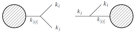
where $B_{\mu\nu}$ is the spin-correlated Born amplitude, while $(\{k\}_{\not{a}\not{b}},k_{c})$ is the radiative kinematics with $k_{a}$ and $k_{b}$ removed and replaced by $k_{c}$. The first two lines of Eq. (38) are pictorially represented in the left and right panels of Figure 1, respectively, while the third line is obtained from the second upon $i\leftrightarrow j$ exchange.

Figure 1: Final-state (left) and initial-state (right) splittings.

2.3.3 Soft-collinear limit

In the soft-collinear ${\bf S}_{i}\,{\bf C}_{ij}$ limit, final-state gluon $i$ becomes both soft and collinear to initial- or final-state parton $j$. The corresponding kernel is

$${\bf S}_{i}\,{\bf C}_{ij}\,R\,=\,{\bf C}_{ij}\,{\bf S}_{i}\,R\,=\,\mathcal{N}_{1}\,2\,C_{f_{j}}\,\mathcal{I}_{jr}^{(i)}\,B(\{k\}_{\not{i}})\,,$$ (39)

where $C_{f_{j}}=C_{A}\,\delta_{f_{j}g}+C_{F}\,\delta_{f_{j}\{q,\bar{q}\}}$ is the SU($N_{c}$) Casimir operator associated to flavour $f_{j}$, and $f_{j}=f_{[ij]}$ since $i$ is a gluon.

For later convenience, we define hard-collinear kernels upon subtracting from the collinear Altarelli-Parisi kernels in Eq. (2.3.2) their respective soft limits: for a final-state splitting, both collinear siblings $i$ and $j$ can give rise to a soft singularity, thus

$$P^{{\rm\,hc}}_{ij,\rm F}(z_{i}) \equiv \big{(}1-\,{\bf S}_{i}-\,{\bf S}_{j}\big{)}\,P_{ij}(z_{i})$$ (40)

$$= \delta_{f_{i}g}\delta_{f_{j}g}\,2\,C_{A}\,z_{i}\,z_{j}+\delta_{\{f_{i}f_{j}\}\{q\bar{q}\}}\,T_{R}\left(1-\frac{2\,z_{i}z_{j}}{1-\epsilon}\right)$$

$$+\,\delta_{f_{i}\{q,\bar{q}\}}\delta_{f_{j}g}\,C_{F}(1-\epsilon)\,z_{j}+\delta_{f_{i}g}\delta_{f_{j}\{q,\bar{q}\}}\,C_{F}(1-\epsilon)\,z_{i}\,,$$

while for an initial-state splitting just one of the two, $i$, can be soft, so

$$P_{[ij]i,\rm I}^{{\rm\,hc}}(x_{[ij]}) \equiv x_{[ij]}\big{(}1-\,{\bf S}_{i}\big{)}\,\frac{P_{[ij]i}(x_{[ij]})}{x_{[ij]}}$$

$$= \delta_{f_{[ij]}g}\delta_{f_{i}g}\,2C_{A}\biggl{[}\frac{x_{i}}{x_{[ij]}}+x_{[ij]}x_{i}\biggr{]}+\delta_{\{f_{[ij]}f_{i}\}\{q\bar{q}\}}\,T_{R}\biggl{[}1-\frac{2\ x_{[ij]}x_{i}}{1-\epsilon}\biggr{]}$$

$$+\,\delta_{f_{[ij]}\{q,\bar{q}\}}\delta_{f_{i}g}\,C_{F}(1-\epsilon)\,x_{i}+\delta_{f_{[ij]}g}\delta_{f_{i}\{q,\bar{q}\}}\,C_{F}\biggl{[}2\frac{x_{i}}{x_{[ij]}}+(1-\epsilon)\,x_{[ij]}\biggr{]}\,.$$

In analogy with Eq. (34), we introduce

$$P_{ab,\star}^{\mu\nu,{\rm\,hc}}(\xi) = P_{ab,\star}^{{\rm\,hc}}(\xi)\,\big{(}\!-\!g^{\mu\nu}\big{)}+Q_{ab,\star}(\xi)\left[-g^{\mu\nu}+(d-2)\,\frac{\widetilde{k}_{\star}^{\mu}\,\widetilde{k}_{\star}^{\nu}}{\widetilde{k}_{\star}^{2}}\right]\,.$$ (42)

2.4 Phase-space mappings and counterterm definitions

Although the candidate counterterm locally reproduces all real phase-space singularities, it embodies Born matrix elements that are evaluated with kinematics that either do not satisfy $n$-body momentum conservation (in the soft case, $\{k\}_{\not{i}}$), or feature an off-shell leg (in the collinear case, ($\{k\}_{\not{a}\not{b}},k_{c}$)). Conversely, it is desirable that the Born matrix elements appearing in counterterms have a physical (i.e. on-shell and momentum conserving) $n$-body kinematics for all choices of the ${n+1}$ radiative momenta, and not only for specific singular configurations, whence a kinematic mapping of momenta is required. In turn, such a mapping operation entails a factorisation of the $({n+1})$-body phase space $d\Phi_{n+1}$ into a remapped $n$-body phase space $d\Phi_{n}$ times a single-radiative measure $d\Phi_{\rm rad}$, which allows the analytic integration of the radiative degrees of freedom at fixed underlying Born kinematics.

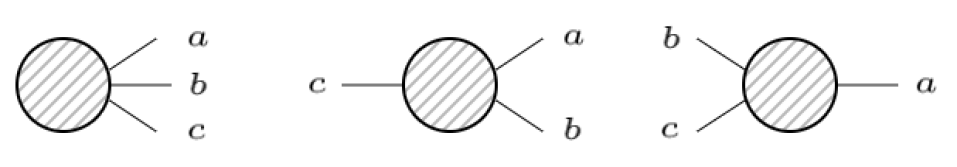
A convenient way of achieving phase-space factorisation is through Catani-Seymour dipole mappings Catani:1996vz , in which a triplet of massless momenta $k_{a}$, $k_{b}$, and $k_{c}$ (the emitted, emitter, and recoiler parton, respectively) are mapped onto a dipole of Born-level momenta $\bar{k}_{b}^{(abc)}$ and $\bar{k}_{c}^{(abc)}$, according to

$$\theta_{{a}\in{\rm F}}\,\theta_{{b}\in{\rm F}}\,\theta_{{c}\in{\rm F}}:\qquad\bar{k}_{b}^{(abc)}+\bar{k}_{c}^{(abc)}\,=\,k_{a}+k_{b}+k_{c}\,,$$

$$\theta_{{a}\in{\rm F}}\,\theta_{{b}\in{\rm F}}\,\theta_{{c}\in{\rm I}}:\qquad\bar{k}_{b}^{(abc)}-\bar{k}_{c}^{(abc)}\,=\,k_{a}+k_{b}-k_{c}\,,$$

$$\theta_{{a}\in{\rm F}}\,\theta_{{b}\in{\rm I}}\,\theta_{{c}\in{\rm I}}:\qquad\sum_{\begin{subarray}{c}i\in\rm F\\ i\neq a\end{subarray}}\,\bar{k}_{i}^{(abc)}-\bar{k}_{b}^{(abc)}-\bar{k}_{c}^{(abc)}\,=\,\sum_{\begin{subarray}{c}i\in\rm F\\ i\neq a\end{subarray}}\,k_{i}+k_{a}-k_{b}-k_{c}\,.$$ (43)

The three assignments are represented pictorially in Figure 2; details on the mappings, parametrisations and corresponding phase-space factorisation are given in Appendix B.

Figure 2: Final-final (left), final-initial (middle), and initial-initial (right) dipoles.

There is ample freedom in the choice of mapping dipoles, as long as this is compatible with the locality of subtraction: in particular, the choice can be adapted to the identity of the partons involved in the different singular kernels. In the soft limit, each eikonal kernel $\mathcal{I}_{kl}^{(i)}$ leads naturally to the choice $(abc)=(ikl)$ or $(abc)=(ilk)$, while in the collinear limits the most natural mapping involves the splitting partons and the recoiler, $(abc)=(ijr)$ or $(abc)=(irj)$. Denoting mapped limits with a bar, we thus define the soft counterterm to be

$$\overline{\bf S}_{i}\,R = -\,2\,\mathcal{N}_{1}\sum_{k\neq i}\sum_{\begin{subarray}{c}l\neq i\\ l<k\end{subarray}}\mathcal{I}_{kl}^{(i)}\bigg{[}\big{(}\theta_{{k}\in{\rm I}}\,\theta_{{l}\in{\rm I}}+\theta_{{k}\in{\rm F}}\,\theta_{{l}\in{\rm I}}+\theta_{{k}\in{\rm F}}\,\theta_{{l}\in{\rm F}}\big{)}\,\bar{B}^{(ikl)}_{kl}+\theta_{{k}\in{\rm I}}\,\theta_{{l}\in{\rm F}}\,\bar{B}^{(ilk)}_{kl}\bigg{]}\,,\qquad$$ (44)

where $\bar{B}_{\dots}^{(abc)}\equiv B_{\dots}(\{\bar{k}\}^{(abc)})$. As for collinear and soft-collinear kernels, we define

$$\overline{\bf C}_{ij}\,R = \frac{\mathcal{N}_{1}}{s_{ij}}\,\Bigg{[}\theta_{{i}\in{\rm F}}\,\theta_{{j}\in{\rm F}}\,P_{ij,\rm F}^{\mu\nu}(z)\,\bar{B}^{(ijr)}_{\mu\nu}$$ (45)

$$\qquad+\,\theta_{{i}\in{\rm F}}\,\theta_{{j}\in{\rm I}}\,\frac{P_{[ij]i,\rm I}^{\mu\nu}(x)}{x}\,\Big{(}\theta_{{r}\in{\rm F}}\,\bar{B}^{(irj)}_{\mu\nu}+\theta_{{r}\in{\rm I}}\,\bar{B}^{(ijr)}_{\mu\nu}\Big{)}$$

$$\qquad+\,\theta_{{j}\in{\rm F}}\,\theta_{{i}\in{\rm I}}\,\frac{P_{[ji]j,\rm I}^{\mu\nu}(x)}{x}\,\Big{(}\theta_{{r}\in{\rm F}}\,\bar{B}^{(jri)}_{\mu\nu}+\theta_{{r}\in{\rm I}}\,\bar{B}^{(jir)}_{\mu\nu}\Big{)}\Bigg{]}\,,\leavevmode\nobreak\$$

$$\overline{\bf S}_{i}\,\overline{\bf C}_{ij}\,R = \mathcal{N}_{1}\,2\,C_{f_{j}}\,\mathcal{I}_{jr}^{(i)}\Bigg{[}\theta_{{j}\in{\rm F}}\,\bar{B}^{(ijr)}+\theta_{{j}\in{\rm I}}\,\Big{(}\frac{\theta_{{r}\in{\rm F}}}{1-z}\,\bar{B}^{(irj)}+\theta_{{r}\in{\rm I}}\,(1-v)\,\bar{B}^{(ijr)}\Big{)}\Bigg{]}\,,$$ (46)

where the soft-collinear contributions for $j\in\rm I$ feature kinematical factors, written in terms of variables $z$ and $v$ defined in Appendix B, whose purpose is to reconstruct the hard-collinear kernels of Eq. (2.3.3):

$$\overline{\bf HC}_{ij}\,R \equiv (1-\overline{\bf S}_{i}-\overline{\bf S}_{j})\,\overline{\bf C}_{ij}\,R$$ (47)

$$= \frac{\mathcal{N}_{1}}{s_{ij}}\,\Bigg{[}\theta_{{i}\in{\rm F}}\,\theta_{{j}\in{\rm F}}\,P_{ij,\rm F}^{\mu\nu,{\rm\,hc}}(z)\,\bar{B}^{(ijr)}_{\mu\nu}$$

$$\hskip 17.07164pt+\,\theta_{{i}\in{\rm F}}\,\theta_{{j}\in{\rm I}}\,\frac{P_{[ij]i,\rm I}^{\mu\nu,{\rm\,hc}}(x)}{x}\,\Big{(}\theta_{{r}\in{\rm F}}\,\bar{B}^{(irj)}_{\mu\nu}+\theta_{{r}\in{\rm I}}\,\bar{B}^{(ijr)}_{\mu\nu}\Big{)}$$

$$\hskip 17.07164pt+\,\theta_{{j}\in{\rm F}}\,\theta_{{i}\in{\rm I}}\,\frac{P_{[ji]j,\rm I}^{\mu\nu,{\rm\,hc}}(x)}{x}\,\Big{(}\theta_{{r}\in{\rm F}}\,\bar{B}^{(jri)}_{\mu\nu}+\theta_{{r}\in{\rm I}}\,\bar{B}^{(jir)}_{\mu\nu}\Big{)}\Bigg{]}\,,$$

where we have defined $\overline{\bf S}_{j}\,\overline{\bf C}_{ij}\equiv\overline{\bf S}_{j}\,\overline{\bf C}_{ji}$. It can be checked (see Appendix C) that the definitions in Eqs. (44 - 46) satisfy the following set of consistency relations

$${\bf S}_{i}\,\overline{\bf S}_{i}\,R\,= \,\,{\bf S}_{i}\,R\,, {\bf C}_{ij}\,\overline{\bf C}_{ij}\,R\,= \,\,{\bf C}_{ij}\,R\,,$$

$${\bf S}_{i}\,\overline{\bf S}_{i}\,\overline{\bf C}_{ij}\ R\,= \,\,{\bf S}_{i}\,\overline{\bf C}_{ij}\,R\,, {\bf C}_{ij}\,\overline{\bf S}_{i}\,\overline{\bf C}_{ij}\,R\,= \,\,{\bf C}_{ij}\,\overline{\bf S}_{i}\,R\,,$$ (48)

ensuring that the application of the mappings detailed above preserves the local cancellation of singularities. This leads to defining the sought local counterterm $K$ as

$$K \equiv \sum_{i}\sum_{j\neq i}K_{ij}\,,\qquad K_{ij}\;\equiv\;\Big{[}\overline{\bf S}_{i}+\overline{\bf C}_{ij}-\overline{\bf S}_{i}\,\overline{\bf C}_{ij}\Big{]}\,R\,\mathcal{W}_{ij}\,,$$ (49)

where, introducing the collective notation $\overline{\bf L}=\overline{\bf S}_{i},\,\overline{\bf C}_{ij},\,\overline{\bf S}_{i}\,\overline{\bf C}_{ij}$, we have defined $\overline{\bf L}_{\,}R\,\mathcal{W}_{ij}\equiv(\overline{\bf L}_{\,}R)\,(\overline{\bf L}_{\,}\mathcal{W}_{ij})$. The definition in Eq. (49) is thus complete only after specifying the action $\overline{\bf L}_{\,}\mathcal{W}_{ij}$ of the barred limits on sector functions. The simplest choice is $\overline{\bf L}_{\,}\mathcal{W}_{ab}\equiv{\bf L}^{\,}\mathcal{W}_{ab}$, resulting in

$$R-K = \sum_{i}\sum_{j\neq i}\Big{[}R\,\mathcal{W}_{ij}-K_{ij}\Big{]}\,=\,\rm{finite}\,.$$ (50)

With this choice, however, the quantity $K_{ij}$ defined in Eq. (49) features spurious singularities in the collinear ${\bf C}_{ir}$ and ${\bf C}_{jr}$ limits, which are not present in $R\,\mathcal{W}_{ij}$. Such singularities, generated by the denominators of the Altarelli-Parisi kernels, drop out only in the sum of mirror sectors $\mathcal{W}_{ij}+\mathcal{W}_{ji}$, ensuring the finiteness of $R-K$. One could envisage removing spurious singularities at the level of the single $\mathcal{W}_{ij}$ partition, which entails redefining the action of the barred limits on sector functions. For instance, it is straightforward to check that by choosing

$$\overline{\mathcal{W}}_{\textrm{s},ij} \equiv \overline{\bf S}_{i}\,\mathcal{W}_{ij}\,\equiv\,\theta_{{i}\in{\rm F}}\,\frac{1/w_{ij}}{\sum\limits_{l\neq i}1/w_{il}}\,,$$

$$\overline{\mathcal{W}}_{\textrm{c},ij} \equiv \overline{\bf C}_{ij}\,\mathcal{W}_{ij}\,\equiv\,\theta_{{i}\in{\rm F}}\left(\theta_{{j}\in{\rm F}}\frac{e_{j}\,w_{jr}}{e_{i}\,w_{ir}+e_{j}\,w_{jr}}+\theta_{{j}\in{\rm I}}\right)\,,$$

$$\overline{\mathcal{W}}_{\textrm{sc},ij} \equiv \overline{\bf S}_{i}\,\overline{\bf C}_{ij}\,\mathcal{W}_{ij}\,\equiv\,\theta_{{i}\in{\rm F}}\,,$$ (51)

one achieves for all $ij$ pairs

$$R\,\mathcal{W}_{ij}-K_{ij}\,=\,\big{(}1-\overline{\bf S}_{i}\big{)}\big{(}1-\overline{\bf C}_{ij}\big{)}\,R\,\mathcal{W}_{ij}\,=\,\rm{finite}\,.$$ (52)

Another possibility, which preserves the flexibility of the numerical implementation of the method reducing the number of sectors, is to introduce symmetrised sector functions in the first place

$$\mathcal{Z}_{ij} \equiv \mathcal{W}_{ij}+\mathcal{W}_{ji}\,,$$ (53)

along with

$$\mathcal{Z}_{{\rm s},\,ij} \equiv \overline{\bf S}_{i}\,\mathcal{Z}_{ij}\;\equiv\;\overline{\bf S}_{i}\,\mathcal{W}_{ij}\,=\,\theta_{{i}\in{\rm F}}\,\frac{1/w_{ij}}{\sum\limits_{l\neq i}1/w_{il}}\,,\qquad\mathcal{Z}_{{\rm s},\,ji}\;\equiv\;\overline{\bf S}_{j}\,\mathcal{Z}_{ij}\,=\,\theta_{{j}\in{\rm F}}\,\frac{1/w_{ij}}{\sum\limits_{l\neq j}1/w_{jl}}\,,$$

$$\mathcal{Z}_{{\rm c},\,ij} \equiv \overline{\bf C}_{ij}\,\mathcal{Z}_{ij}\;\equiv\;\overline{\bf C}_{ij}\,\mathcal{W}_{ij}+\overline{\bf C}_{ij}\,\mathcal{W}_{ji}\,=\,1-\theta_{{i}\in{\rm I}}\,\theta_{{j}\in{\rm I}}\,,$$

$$\mathcal{Z}_{{\rm sc},\,ij} \equiv \overline{\bf S}_{i}\,\overline{\bf C}_{ij}\,\mathcal{Z}_{ij}\;\equiv\;\overline{\bf S}_{i}\,\overline{\bf C}_{ij}\,\mathcal{W}_{ij}\,=\,\theta_{{i}\in{\rm F}}\,,\qquad\mathcal{Z}_{{\rm sc},\,ji}\;\equiv\;\overline{\bf S}_{j}\,\overline{\bf C}_{ij}\,\mathcal{Z}_{ij}\,=\,\theta_{{j}\in{\rm F}}\,.$$ (54)

We can then define the symmetrised counterterms

$$K_{\{ij\}} \equiv K_{ij}+K_{ji}\,=\,\Big{[}\overline{\bf S}_{i}+\overline{\bf S}_{j}+\overline{\bf C}_{ij}\big{(}1-\overline{\bf S}_{i}-\overline{\bf S}_{j}\big{)}\Big{]}\,R\,\mathcal{Z}_{ij}$$

$$= \big{(}\overline{\bf S}_{i}\,R\big{)}\mathcal{Z}_{{\rm s},ij}+\big{(}\overline{\bf S}_{j}\,R\big{)}\mathcal{Z}_{{\rm s},ji}+\overline{\bf HC}_{ij}\,R\,,$$

$$K = \sum_{i}\sum_{j<i}K_{\{ij\}}\,,$$ (55)

satisfying

$$R\,\mathcal{Z}_{ij}-K_{\{ij\}} = \Big{[}\big{(}1-\overline{\bf C}_{ij}\big{)}\big{(}1-\overline{\bf S}_{i}-\overline{\bf S}_{j}\big{)}\Big{]}\,R\,\mathcal{Z}_{ij}\,=\,\rm{finite}\,,$$

$$R-K = \sum_{i}\sum_{j<i}\Big{[}R\,\mathcal{Z}_{ij}-K_{\{ij\}}\Big{]}\,=\,\rm{finite}\,.$$ (56)

We stress that, in any case, the sum rules in (14 - 16) allow to get rid of sector functions and to write the local counterterm purely as a collection of universal soft and collinear NLO kernels:

$$K = \sum_{i}\bigg{[}\overline{\bf S}_{i}\,R+\sum_{j<i}\,\overline{\bf HC}_{ij}\,R\bigg{]}\,.$$ (57)

2.5 Local counterterms with damping factors

At this stage, we have all the ingredients to build a counterterm $K$ which, along with its integration over the radiative phase space, achieves a local subtraction. Nonetheless, it is worth investigating a systematic optimisation of the above definitions, with a view to improving the efficiency of the method. Since the subtraction procedure is necessary only in the IRC corners of the phase space, one is allowed to tune the counterterm contribution in the non-singular regions, thereby reducing numerical instabilities. This is customarily achieved in the literature by introducing parameters (such as the $\alpha$ parameter in CS Nagy:2003tz , and the $\delta$ and $\xi_{\rm cut}$ parameters in FKS Frixione:1995ms ) that set a hard boundary to the phase space allowed for counterterms. The enhanced numerical stability of this procedure in general comes at the price of a more cumbersome analytic counterterm integration, which may become untenable at NNLO.

What we propose in this article is instead to multiply the local counterterms in Eqs. (44 - 46) by means of smooth damping factors (as opposed to hard step functions) in order to gradually turn them off away from the singular regions. Although one has some freedom in constructing such damping factors, provided the validity of Eqs. (2.4) is not spoiled, it is particularly convenient to define them as powers, with tunable exponents, of the kinematic invariants proper of the chosen phase-space parametrisation. By doing so, one is essentially including in a controlled way subleading power terms in the normal variables through which the IRC kernels are already written. As a result, the presence of damping factors does not affect the complexity of the analytic integrations, which is crucial for exporting this optimisation to higher perturbative orders. The explicit dependence of (the finite part of) the integrated counterterms upon the damping parameters, namely the above-mentioned tunable exponents, must cancel against an analogous dependence in the local counterterms, which is known to offer a powerful handle to check the numerical implementation of the subtraction method.

We start by including damping factors in the soft counterterm, Eq. (44):

$$\overline{\bf S}_{i}\,R = -\,2\,\mathcal{N}_{1}\sum_{k\neq i}\sum_{\begin{subarray}{c}l\neq i\\ l<k\end{subarray}}\mathcal{I}_{kl}^{(i)}\bigg{\{}\theta_{{k}\in{\rm F}}\,(1-z)^{\alpha}\,\Big{[}\theta_{{l}\in{\rm F}}\,(1-y)^{\alpha}+\theta_{{l}\in{\rm I}}\,x^{\alpha}\Big{]}\bar{B}^{(ikl)}_{kl}$$ (58)

$$\hskip 82.51299pt+\,\theta_{{k}\in{\rm I}}\,x^{\alpha}\,\Big{[}\theta_{{l}\in{\rm F}}\,(1-z)^{\alpha}\,\bar{B}^{(ilk)}_{kl}+\theta_{{l}\in{\rm I}}\,\bar{B}^{(ikl)}_{kl}\Big{]}\bigg{\}}\,\,,$$

where $\alpha\geq 0$, and the $x$, $y$, $z$ kinematic variables are those associated to the $(ikl)$ or $(ilk)$ phase-space mappings, i.e. they are different for each term in the eikonal double sum. In detail, they are defined as in Eq. (100), Eq. (107), Eq. (114) for $(kl)=\rm FF,FI,IF,II$, respectively. The case with no damping, Eq. (44), is simply obtained setting $\alpha=0$.

As far as collinear and soft-collinear contributions are concerned, Eq. (45) and Eq. (46) are modified as

$$\overline{\bf C}_{ij}\,R = \frac{\mathcal{N}_{1}}{s_{ij}}\,\Bigg{\{}\;\theta_{{i}\in{\rm F}}\,\theta_{{j}\in{\rm F}}\,P_{ij,\rm F}^{\mu\nu}(z)\,\Big{[}\theta_{{r}\in{\rm F}}\,(1-y)^{\beta}+\theta_{{r}\in{\rm I}}\,x^{\beta}\,\Big{]}\,\bar{B}^{(ijr)}_{\mu\nu}$$ (59)

$$\hskip 19.91692pt+\,\theta_{{i}\in{\rm F}}\,\theta_{{j}\in{\rm I}}\,\frac{P_{[ij]i,\rm I}^{\mu\nu}(x)}{x}\,\Big{[}\theta_{{r}\in{\rm F}}\,(1-z)^{\gamma}\,\bar{B}^{(irj)}_{\mu\nu}+\theta_{{r}\in{\rm I}}\,(1-v)^{\gamma}\,\bar{B}^{(ijr)}_{\mu\nu}\Big{]}$$

$$\hskip 19.91692pt+\,\theta_{{j}\in{\rm F}}\,\theta_{{i}\in{\rm I}}\,\frac{P_{[ji]j,\rm I}^{\mu\nu}(x)}{x}\,\Big{[}\theta_{{r}\in{\rm F}}\,(1-z)^{\gamma}\,\bar{B}^{(jri)}_{\mu\nu}+\theta_{{r}\in{\rm I}}\,(1-v)^{\gamma}\,\bar{B}^{(jir)}_{\mu\nu}\Big{]}\Bigg{\}}\,,\qquad$$

$$\overline{\bf S}_{i}\,\overline{\bf C}_{ij}\,R = \mathcal{N}_{1}\,2\,C_{f_{j}}\,\mathcal{I}_{jr}^{(i)}\bigg{\{}\;\theta_{{j}\in{\rm F}}\,(1-z)^{\alpha}\,\Big{[}\theta_{{r}\in{\rm F}}\,(1-y)^{\beta}+\theta_{{r}\in{\rm I}}\,x^{\beta}\Big{]}\bar{B}^{(ijr)}$$ (60)

$$\hskip 59.75078pt+\,\theta_{{j}\in{\rm I}}\,x^{\alpha}\Big{[}\theta_{{r}\in{\rm F}}\,(1-z)^{\gamma-1}\bar{B}^{(irj)}+\theta_{{r}\in{\rm I}}\,(1-v)^{\gamma+1}\bar{B}^{(ijr)}\Big{]}\bigg{\}}\,,\quad$$

where $\alpha$ is the same exponent appearing in the damped soft counterterm, Eq. (58), while $\beta,\gamma\geq 0$ are relevant for final- and initial-state collinear emission, respectively. The kinematic variables building the damping factors depend on the mapping appearing in the relevant Born matrix element, as in the soft case. The un-damped limits are obtained upon setting $\alpha=\beta=\gamma=0$.

Following the same steps detailed in Appendix C, it can be checked that the damped counterterm definitions in Eqs. (58 - 60) correctly satisfy the consistency relations in Eqs. (2.4). It will be moreover shown in the next Section that, as expected, the $\epsilon$ poles of the integrated counterterms do not feature any dependence on the arbitrary parameters $\alpha,\beta,\gamma$, which thus appear only in the finite part $\mathcal{O}(\epsilon^{0})$.

We point out that the structure of the local counterterm $K$ and of its sector components $K_{ij}$, $K_{\{ij\}}$ given in Eqs. (49, 2.4, 57) is not affected by the presence of damping factors and remains formally valid for arbitrary values of $\alpha,\beta,\gamma$. The damped $\overline{\bf HC}_{ij}\,R$ counterterms can still be written in terms of the hard-collinear kernels $P^{{\rm\,hc}}_{ij,\star}$

$$\overline{\bf HC}_{ij}\,R \equiv (1-\overline{\bf S}_{i}-\overline{\bf S}_{j})\,\overline{\bf C}_{ij}\,R$$

$$= \theta_{{i}\in{\rm F}}\,\theta_{{j}\in{\rm F}}\,\overline{\bf HC}_{ij}^{\,\rm F}\,R+\theta_{{i}\in{\rm F}}\,\theta_{{j}\in{\rm I}}\,\overline{\bf HC}_{ij}^{\,\rm I}\,R+\theta_{{j}\in{\rm F}}\,\theta_{{i}\in{\rm I}}\,\overline{\bf HC}_{ji}^{\,\rm I}\,R\,,$$

$$\overline{\bf HC}_{ij}^{\,\rm F}\,R \equiv \mathcal{N}_{1}\Big{[}\theta_{{r}\in{\rm F}}\,(1-y)^{\beta}+\theta_{{r}\in{\rm I}}\,x^{\beta}\,\Big{]}$$

$$\hskip 14.22636pt\Bigg{[}\frac{P_{ij,\rm F}^{\mu\nu,{\rm hc}}(z)\!}{s_{ij}}\bar{B}^{(ijr)}_{\mu\nu}+2\,\Big{[}C_{\!f_{j}}\mathcal{I}_{jr}^{(i)}\Big{(}\!1\!-\!(1\!-\!z)^{\alpha}\!\Big{)}+C_{\!f_{i}}\mathcal{I}_{ir}^{(j)}(1\!-\!z^{\alpha})\Big{]}\bar{B}^{(ijr)}\!\Bigg{]}\,,$$

$$\overline{\bf HC}_{ij}^{\,\rm I}\,R \equiv \mathcal{N}_{1}\,\Bigg{[}\theta_{{r}\in{\rm F}}\,(1\!-\!z)^{\gamma}\Bigg{(}\!\frac{P_{\![ij]i,\rm I}^{\mu\nu,{\rm hc}}(x)\!}{x\,s_{ij}}\bar{B}^{(irj)}_{\mu\nu}+2C_{\!f_{j}}\,\mathcal{I}_{jr}^{(i)}\frac{1-x^{\alpha}}{1-z}\bar{B}^{(irj)}\!\Bigg{)}$$ (61)

$$\hskip 14.22636pt+\,\theta_{{r}\in{\rm I}}\,(1\!-\!v)^{\gamma}\Bigg{(}\!\frac{P_{\![ij]i,\rm I}^{\mu\nu,{\rm hc}}(x)\!}{x\,s_{ij}}\bar{B}^{(ijr)}_{\mu\nu}+2C_{\!f_{j}}\mathcal{I}_{jr}^{(i)}(1\!-\!x^{\alpha})(1\!-\!v)\bar{B}^{(ijr)}\!\Bigg{)}\!\Bigg{]}\,,$$

which will be integrated in the next Section.

3 Counterterm integration

In order to analytically integrate the counterterms, it is convenient to start from Eq. (57), relying on the kernel definitions in Eqs. (58, 2.5). The counterterm expression is summed over sectors, compatibly with the fact that its integral must reproduce the poles of the virtual matrix element, which is not partitioned. We split $K$ into soft, final-state hard-collinear and initial-state hard-collinear contributions,

$$K\, \equiv \,K_{\rm s}\,+\,K_{{\rm\,hc},\rm F}\,+\,K_{{\rm\,hc},\rm I}\,,$$ (62)

defined as

$$K_{\rm s} \equiv \sum_{i}\,\overline{\bf S}_{i}\,R\,,$$ (63)

$$K_{{\rm\,hc},\rm F} \equiv \sum_{i}\,\sum_{j<i}\,\theta_{{i}\in{\rm F}}\,\theta_{{j}\in{\rm F}}\,\overline{\bf HC}_{ij}^{\,\rm F}\,R\,,$$ (64)

$$K_{{\rm\,hc},\rm I} \equiv \sum_{i}\,\sum_{j<i}\,\Big{[}\theta_{{i}\in{\rm F}}\,\theta_{{j}\in{\rm I}}\,\overline{\bf HC}_{ij}^{\,\rm I}\,R+\theta_{{j}\in{\rm F}}\,\theta_{{i}\in{\rm I}}\,\overline{\bf HC}_{ji}^{\,\rm I}\,R\Big{]}\,.$$ (65)

The phase-space measures used for integration are given and described in full detail in Appendix B, for all cases of initial- and final-state radiation.

We start with the integration of the soft counterterm $K_{\rm s}$ in Eq. (63), yielding

$$\int d\Phi_{n+1}\,\overline{\bf S}_{i}\,R\,=\,$$

$$= -\,2\,\mathcal{N}_{1}\,\frac{\varsigma_{n+1}}{\varsigma_{n}}\,\sum_{k\neq i}\sum_{\begin{subarray}{c}l\neq i\\ l<k\end{subarray}}\,\mathcal{I}_{kl}^{(i)}\,\bigg{[}\theta_{{k}\in{\rm F}}\,\theta_{{l}\in{\rm F}}\,\int d\Phi_{n}^{(ikl)}\!\int d\Phi_{\rm rad}^{(ikl)}\,(1-y)^{\alpha}(1-z)^{\alpha}\,\bar{B}^{(ikl)}_{kl}$$

$$\hskip 110.96574pt+\,\theta_{{k}\in{\rm F}}\,\theta_{{l}\in{\rm I}}\,\int\!\int d\Phi_{n}^{(ikl)}(xk_{l})\,d\Phi_{\rm rad}^{(ikl)}\,x^{\alpha}\,(1-z)^{\alpha}\,\bar{B}^{(ikl)}_{kl}$$

$$\hskip 110.96574pt+\,\theta_{{l}\in{\rm F}}\,\theta_{{k}\in{\rm I}}\,\int\!\int d\Phi_{n}^{(ilk)}(xk_{k})\,d\Phi_{\rm rad}^{(ilk)}\,x^{\alpha}\,(1-z)^{\alpha}\,\bar{B}^{(ilk)}_{kl}$$

$$\hskip 110.96574pt+\,\theta_{{k}\in{\rm I}}\,\theta_{{l}\in{\rm I}}\,\int\!\int d\Phi_{n}^{(ikl)}(xk_{k},k_{l})\,d\Phi_{\rm rad}^{(ikl)}\,x^{\alpha}\,\bar{B}^{(ikl)}_{kl}\bigg{]}$$

$$\equiv -\,2\,\frac{\varsigma_{n+1}}{\varsigma_{n}}\sum_{k\neq i}\sum_{\begin{subarray}{c}l\neq i\\ l<k\end{subarray}}\bigg{\{}\,\theta_{{k}\in{\rm F}}\,\theta_{{l}\in{\rm F}}\,\int d\Phi_{n}^{(ikl)}\,I_{\rm s,\rm F\rm F}^{ikl}\,\bar{B}^{(ikl)}_{kl}$$

$$\hskip 73.97716pt+\,\theta_{{k}\in{\rm F}}\,\theta_{{l}\in{\rm I}}\bigg{[}\!\int\!d\Phi_{n}^{(ikl)}(k_{l})\,I_{\rm s,\rm F\rm I}^{ikl}+\int_{0}^{1}\!\frac{dx}{x}\!\int\!d\Phi_{n}^{(ikl)}(xk_{l})\,J_{\rm s,\rm F\rm I}^{ikl}(x)\!\bigg{]}\bar{B}^{(ikl)}_{kl}$$

$$\hskip 73.97716pt+\,\theta_{{l}\in{\rm F}}\,\theta_{{k}\in{\rm I}}\bigg{[}\!\int\!d\Phi_{n}^{(ilk)}(k_{k})\,I_{\rm s,\rm F\rm I}^{ilk}+\int_{0}^{1}\!\frac{dx}{x}\!\int\!d\Phi_{n}^{(ilk)}(xk_{k})\,J_{\rm s,\rm F\rm I}^{ilk}(x)\!\bigg{]}\bar{B}^{(ilk)}_{kl}$$

$$\hskip 73.97716pt+\,\theta_{{k}\in{\rm I}}\,\theta_{{l}\in{\rm I}}\bigg{[}\!\int\!d\Phi_{n}^{(ikl)\!}(k_{k},k_{l})\,I_{\rm s,\rm I\rm I}^{ikl}+\int_{0}^{1}\!\frac{dx}{x}\!\int\!d\Phi_{n}^{(ikl)\!}(xk_{k},k_{l})\,J_{\rm s,\rm I\rm I}^{ikl}(x)\!\bigg{]}\bar{B}^{(ikl)}_{kl}\bigg{\}}.$$

The expressions for the integrals $I_{\rm s,\star\star}^{iab}$ and $J_{\rm s,\star\star}^{iab}(x)$, are reported in Appendix D.1, where the latter (former) collect $x$-(in)dependent contributions.

Moving to the hard-collinear counterterms $K_{{\rm\,hc},\star}$ in Eqs. (65 - 64), we notice that the azimuthal contribution multiplying $Q_{ab,\star}$ in the collinear kernels vanishes upon integration, hence only unpolarised Altarelli-Parisi kernels need to be integrated. For a final-state $j$, relevant to $K_{{\rm\,hc},\rm F}$, one has

$$\int d\Phi_{n+1}\,\overline{\bf HC}_{ij}^{\,\rm F}\,R\,=\,$$ (67)

$$= \mathcal{N}_{1}\,\frac{\varsigma_{n+1}}{\varsigma_{n}}\,\bigg{[}\theta_{{r}\in{\rm F}}\,\int d\Phi_{n}^{(ijr)}\!\int d\Phi_{\rm rad}^{(ijr)}\,(1-y)^{\beta}+\theta_{{r}\in{\rm I}}\,\int\int d\Phi_{n}^{(ijr)}(xk_{r})\,d\Phi_{\rm rad}^{(ijr)}\,x^{\beta}\bigg{]}$$

$$\hskip 39.83385pt\Bigg{[}\frac{P_{ij,\rm F}^{{\rm hc}}(z)\!}{s_{ij}}+2\,\Big{[}C_{\!f_{j}}\,\mathcal{I}_{jr}^{(i)}\Big{(}1\!-\!(1\!-\!z)^{\alpha}\Big{)}+C_{\!f_{i}}\,\mathcal{I}_{ir}^{(j)}(1\!-\!z^{\alpha})\Big{]}\!\Bigg{]}\bar{B}^{(ijr)}$$

$$\equiv \frac{\varsigma_{n+1}}{\varsigma_{n}}\,\bigg{[}\,\theta_{{r}\in{\rm F}}\!\int\!d\Phi_{n}^{(ijr)}\Big{(}I_{\rm hc,\rm F\rm F}^{ijr}+I_{\rm sc,\rm F\rm F}^{ijr}+I_{\rm sc,\rm F\rm F}^{jir}\Big{)}$$

$$\hskip 22.76219pt+\,\theta_{{r}\in{\rm I}}\!\int\!d\Phi_{n}^{(ijr)}(k_{r})\Big{(}I_{\rm hc,\rm F\rm I}^{ijr}+I_{\rm sc,\rm F\rm I}^{ijr}+I_{\rm sc,\rm F\rm I}^{jir}\Big{)}$$

$$\hskip 22.76219pt+\,\theta_{{r}\in{\rm I}}\,\int_{0}^{1}\frac{dx}{x}\int d\Phi_{n}^{(ijr)}(xk_{r})\,\Big{(}J_{\rm hc,\rm F\rm I}^{ijr}(x)+J_{\rm sc,\rm F\rm I}^{ijr}(x)+J_{\rm sc,\rm F\rm I}^{jir}(x)\Big{)}\bigg{]}\,\bar{B}^{(ijr)}\,,$$

where the contributions proportional to $\theta_{{r}\in{\rm F}}$ or $\theta_{{r}\in{\rm I}}$ correspond to different prescriptions for the position of the recoiler particle. Likewise, the integration of the constituents of $K_{{\rm\,hc},\rm I}$ gives

$$\int d\Phi_{n+1}\,\overline{\bf HC}_{ij}^{\,\rm I}\,R\,=\,$$

$$= \mathcal{N}_{1}\frac{\varsigma_{n+1}}{\varsigma_{n}}\Bigg{[}\theta_{{r}\in{\rm F}}\!\int\!\!\int\!d\Phi_{n}^{(irj)}(xk_{j})\,d\Phi_{\rm rad}^{(irj)}(1\!-\!z)^{\gamma}\Bigg{(}\!\frac{P_{\![ij]i,\rm I}^{{\rm hc}}(x)\!}{x\,s_{ij}}+2C_{\!f_{j}}\mathcal{I}_{jr}^{(i)}\frac{1\!-\!x^{\alpha}}{1\!-\!z}\!\Bigg{)}\bar{B}^{(irj)}$$

$$\hskip 36.98857pt+\,\theta_{{r}\in{\rm I}}\!\int\!\!\int\!d\Phi_{n}^{(ijr)\!}(xk_{j},k_{r})\,d\Phi_{\rm rad}^{(ijr)}(1\!-\!v)^{\gamma}\!\Bigg{(}\!\frac{P_{\![ij]i,\rm I}^{{\rm hc}}(x)\!}{x\,s_{ij}}+2C_{\!f_{j}}\mathcal{I}_{jr}^{(i)}(1\!-\!x^{\alpha})(1\!-\!v)\!\Bigg{)}\bar{B}^{(ijr)}\!\Bigg{]}$$

$$\equiv \frac{\varsigma_{n+1}}{\varsigma_{n}}\bigg{\{}\theta_{{r}\in{\rm F}}\bigg{[}\int_{0}^{1}\!\frac{dx}{x}\!\int\!d\Phi_{n}^{(irj)}(xk_{j})\Big{(}J_{\rm hc,\rm I\rm F}^{irj}(x)+J_{\rm sc,\rm I\rm F}^{irj}(x)\Big{)}+\int\!d\Phi_{n}^{(irj)}(k_{j})\,I_{\rm sc,\rm I\rm F}^{irj}\bigg{]}\bar{B}^{(irj)}$$

$$\hskip 22.76219pt+\,\theta_{{r}\in{\rm I}}\,\bigg{[}\int_{0}^{1}\!\frac{dx}{x}\!\int\!d\Phi_{n}^{(ijr)\!}(xk_{j},k_{r})\Big{(}J_{\rm hc,\rm I\rm I}^{ijr}(x)+J_{\rm sc,\rm I\rm I}^{ijr}(x)\Big{)}+\int\!d\Phi_{n}^{(ijr)\!}(k_{j},k_{r})\,I_{\rm sc,\rm I\rm I}^{ijr}\bigg{]}\bar{B}^{(ijr)}\!\Bigg{\}}.$$

All integrals $I^{iab}_{\rm hc/\rm sc,\star\star}$ and $J^{iab}_{\rm hc/\rm sc,\star\star}(x)$ featuring in the previous equations are collected in Appendix D.2.

In order to obtain the integrated counterterms $I$ and $J$, two final steps are required. First, all various Born-level parametrisations are identified, as the corresponding phase spaces have identical support, which amounts to the following relabelings:

$$\{\bar{k}\}^{(abc)}\,\to\,\{k\}\,,\qquad\qquad d\Phi_{n}^{(abc)}\,\to\,d\Phi_{n}\,,\qquad\qquad\bar{B}^{(abc)}_{\dots}\,\to\,B_{\dots}\,.$$ (69)

Then, sums over $(n+1)$-body labels must be converted into Born-level sums. When a final-state gluon $i$ is removed, relevant to the soft case, one has

$$\frac{\varsigma_{n+1}}{\varsigma_{n}}\,\sum_{i\in\rm F}\,\delta_{f_{i}g} = 1\,;$$ (70)

when two final-state particles $i$ and $j$ are replaced by the parent particle $p$, the sums over $i$ and $j$ can be recast as a sum over $p$ according to

$$\frac{\varsigma_{n+1}}{\varsigma_{n}}\,\sum_{i\in\rm F}\sum_{\begin{subarray}{c}j\in\rm F\\ j<i\end{subarray}}\,\delta_{\{f_{i}f_{j}\}\{q\bar{q}\}} = N_{f}\,\sum_{p\in\rm F}\,\delta_{f_{p}g}\,,$$

$$\frac{\varsigma_{n+1}}{\varsigma_{n}}\,\sum_{i\in\rm F}\sum_{\begin{subarray}{c}j\in\rm F\\ j<i\end{subarray}}\,\left(\delta_{f_{i}\{q,\bar{q}\}}\delta_{f_{j}g}+\delta_{f_{j}\{q,\bar{q}\}}\delta_{f_{i}g}\right) = \sum_{p\in\rm F}\,\delta_{f_{p}\{q,\bar{q}\}}\,,$$

$$\frac{\varsigma_{n+1}}{\varsigma_{n}}\,\sum_{i\in\rm F}\sum_{\begin{subarray}{c}j\in\rm F\\ j<i\end{subarray}}\,\delta_{f_{i}g}\,\delta_{f_{j}g} = \frac{1}{2}\sum_{p\in\rm F}\,\delta_{f_{p}g}\,,$$ (71)

where $N_{f}$ is the number of light active flavours; in the case of a final-state particle $i$ and an initial-state particle $j$ replaced by the resulting initial-state particle $a$, the relevant relations are

$$\frac{\varsigma_{n+1}}{\varsigma_{n}}\,\sum_{i\in\rm F}\sum_{j\in\rm I}\,\delta_{\{f_{[ij]}f_{i}\}\{q\bar{q}\}} = \sum_{a\in\rm I}\,\delta_{f_{a}g}\,,$$

$$\frac{\varsigma_{n+1}}{\varsigma_{n}}\,\sum_{i\in\rm F}\sum_{j\in\rm I}\,\delta_{f_{[ij]}\{q,\bar{q}\}}\,\delta_{f_{i}g} = \sum_{a\in\rm I}\,\delta_{f_{a}\{q,\bar{q}\}}\,,$$

$$\frac{\varsigma_{n+1}}{\varsigma_{n}}\,\sum_{i\in\rm F}\sum_{j\in\rm I}\,\delta_{f_{[ij]}g}\,\delta_{f_{i}\{q,\bar{q}\}} = \sum_{a\in\rm I}\,\delta_{f_{a}\{q,\bar{q}\}}\,,$$

$$\frac{\varsigma_{n+1}}{\varsigma_{n}}\,\sum_{i\in\rm F}\sum_{j\in\rm I}\,\delta_{f_{[ij]}g}\,\delta_{f_{i}g} = \sum_{a\in\rm I}\,\delta_{f_{a}g}\,.$$ (72)

After such a procedure, all above integrals are naturally written in terms of Born-level quantities. With $\star=\rm F,\rm I$, one has

$$I_{\rm s,\star\star}^{abc} \to I_{\rm s,\star\star}\left(s_{bc}\right)\,,\qquad J_{\rm s,\star\star}^{abc}(x)\,\to\,J_{\rm s,\star\star}\left(s_{bc},x\right)\,,$$

$$I_{\rm sc,\star\star}^{abc} \to 2\,C_{f_{b}}\,I_{\rm sc,\star\star}\left(s_{bc}\right)\,,\qquad J_{\rm sc,\star\star}^{abc}(x)\,\to\,2\,C_{f_{b}}\,J_{\rm sc,\star\star}\left(s_{bc},x\right)\,,$$

$$I_{\rm hc,\rm F\star}^{abc} \to \delta_{f_{b}g}\,\bigg{[}\frac{1}{2}\,I_{\rm hc,\rm F\star}^{({\rm 2g})}\left(s_{bc}\right)+N_{f}\,I_{\rm hc,\rm F\star}^{({\rm 0g})}\left(s_{bc}\right)\bigg{]}+\delta_{f_{b}\{q,\bar{q}\}}\,I_{\rm hc,\rm F\star}^{({\rm 1g})}\left(s_{bc}\right)\,,$$

$$J_{\rm hc,\rm F\star}^{abc}(x) \to \delta_{f_{b}g}\,\bigg{[}\frac{1}{2}\,J_{\rm hc,\rm F\star}^{({\rm 2g})}\left(s_{bc},x\right)+N_{f}\,J_{\rm hc,\rm F\star}^{({\rm 0g})}\left(s_{bc},x\right)\bigg{]}+\delta_{f_{b}\{q,\bar{q}\}}\,J_{\rm hc,\rm F\star}^{({\rm 1g})}\left(s_{bc},x\right)\,,$$

$$J_{\rm hc,\rm I\star}^{abc}(x) \to \delta_{f_{b}g}\,\bigg{[}J_{\rm hc,\rm I\star}^{({\rm 2g})}\left(s_{bc},x\right)+J_{\rm hc,\rm I\star}^{({\rm 0g})}\left(s_{bc},x\right)\bigg{]}+\delta_{f_{b}\{q,\bar{q}\}}\,J_{\rm hc,\rm I\star}^{({\rm 1g})}\left(s_{bc},x\right)\,,$$ (73)

where, on the right-hand sides, $b$ and $c$ are Born-level labels. The quantities $I_{\rm s/sc/hc,\star\star}(s)$ and $J_{\rm s/sc/hc,\star\star}(s,x)$ appearing on the right-hand side of the above identifications are collected in Appendices D.1 and D.2.

4 NLO massless subtraction formula

We are now in the position of verifying that the integrated counterterm correctly reproduces all virtual $\epsilon$ poles, thus providing a valid local subtraction formula for generic NLO processes without massive colourful particles. We separately consider the cases of 0, 1, 2 initial-state QCD partons, relevant to lepton-lepton, lepton-hadron, and hadron-hadron collisions, respectively. For these three process categories, we dub the counterterm $K$ as $K^{\rm F}$, $K^{\rm IF}$, and $K^{\rm IIF}$, respectively.

4.1 No initial-state QCD partons

The counterterm for leptonic processes is

$$K^{\rm F} = K_{\rm s}+\theta_{{r}\in{\rm F}}\,K_{{\rm\,hc},\rm F}\,,$$ (74)

where $K_{\rm s}$ and $K_{{\rm\,hc},\rm F}$ are defined in Eqs. (63, 64), and the notation makes explicit the fact that the emitting dipole $jr$ appearing in the hard-collinear kernels is bound to belong to the final state.

The integration over the radiative phase space, up to $\mathcal{O}(\epsilon)$, yields

$$I^{\rm F}\,=\,I_{\text{poles}}+I^{\rm F}_{\text{fin}}\,,$$ (75)

where

$$I_{\text{poles}} = \frac{\alpha_{\mbox{\tiny{S}}}}{2\pi}\bigg{[}\frac{1}{\epsilon^{2}}\,\sum_{j}C_{f_{j}}\,B+\frac{1}{\epsilon}\Big{(}\sum_{j}\gamma_{j}\,B+\sum_{c,d\neq c}\!{\rm L}_{cd}\,B_{cd}\Big{)}\bigg{]}\,,$$ (76)

$$I^{\rm F}_{\text{fin}} = \frac{\alpha_{\mbox{\tiny{S}}}}{2\pi}\bigg{\{}\Big{[}\sum_{k\in\rm F}\phi_{k}-\sum_{j}\gamma_{j}^{{\rm\,hc}}\,{\rm L}_{jr}\Big{]}\,B+\sum_{c,d\neq c}{\rm L}_{cd}\,\Big{(}2-\frac{1}{2}\,{\rm L}_{cd}\Big{)}\,B_{cd}$$

$$\hskip 14.22636pt+\,2\,A_{2}(\alpha)\,\Big{[}\sum_{j}\,C_{f_{j}}\,{\rm L}_{jr}\,B+\sum_{c,d\neq c}{\rm L}_{cd}\,B_{cd}\Big{]}+\sum_{k\in\rm F}\gamma^{{\rm\,hc}}_{k}\,A_{2}(\beta)\,B$$

$$\hskip 14.22636pt+\Big{[}A_{2}(\alpha)\Big{(}A_{2}(\alpha)-2\,A_{2}(\beta)\Big{)}-A_{3}(\alpha)\Big{]}\,\sum_{j}C_{f_{j}}\,B\bigg{\}}\,.$$

We have introduced some short-hand notation for logarithms, ${\rm L}_{ab}=\ln(s_{ab}/\mu^{2})$, and for anomalous dimensions,

$$\gamma_{a}\,=\,\frac{3}{2}\,C_{F}\,\delta_{f_{a}\{q,\bar{q}\}}+\frac{1}{2}\,\beta_{0}\,\delta_{f_{a}g}\,,\qquad\gamma_{a}^{{\rm\,hc}}\,=\,\gamma_{a}-2\,C_{f_{a}}\,,$$

$$\phi_{a}\,=\,\frac{13}{3}\,C_{F}\,\delta_{f_{a}\{q,\bar{q}\}}+\frac{4}{3}\,\beta_{0}\,\delta_{f_{a}g}+\left(\frac{2}{3}-\frac{7}{2}\,\zeta_{2}\right)\,C_{f_{a}}\,,$$ (77)

where $\beta_{0}=\big{(}11\,C_{A}-4\,T_{R}\,N_{f}\big{)}/3$ is the first coefficient of the QCD beta function, $C_{A}=N_{c}$, $C_{F}=(N_{c}^{2}-1)/(2N_{c})$ and $T_{R}=1/2$. The functions $A_{n}(x)$ are defined in Appendix D.

The poles in Eq. (76) are correctly independent of the damping parameters $\alpha$ and $\beta$, and can be checked to exactly match those of virtual origin, see for instance Catani:1998bh , thus verifying the cancellation of singularities in the first line of Eq. (9). As for the finite contribution, the second and third lines collect the full dependence upon the damping parameters, and cancel out as $\alpha=\beta=0$.

4.2 One initial-state QCD parton

The local counterterm relevant for a reaction with one incoming QCD parton is

$$K^{\rm IF} = K_{\rm s}+\theta_{{r}\in{\rm I}}\,K_{{\rm\,hc},\rm F}+\theta_{{r}\in{\rm F}}\,K_{{\rm\,hc},\rm I}\,,$$ (78)

where the singular kernels are listed in Eqs. (63 - 65). In $K_{{\rm\,hc},\rm I}$ one assigns a final-state recoiler since the only initial-state coloured parton is identified with $j$. As for $K_{{\rm\,hc},\rm F}$, one could assign a final-state recoiler only if the process featured at least one massless colourful parton in the final state at Born level, on top of the final-state emitter $j$. Identifying the recoiler with the initial-state colourful parton is instead always allowed.

The integration over the radiative phase space up to $\mathcal{O}(\epsilon)$ gives

$$\int d\Phi_{n+1}\,K^{\rm IF} = \int d\Phi_{n}(k_{a})\,\Big{(}I^{\rm F}+I^{\rm I}_{\text{fin}}\Big{)}+\int_{0}^{1}\frac{dx}{x}\int d\Phi_{n}(xk_{a})\,J^{\rm I}(x)\,,$$ (79)

where $I^{\rm F}$ is the same as in Eq. (75), while $I^{\rm I}_{\text{fin}}$ is a purely finite contribution reading

$$I^{\rm I}_{\text{fin}} = \frac{\alpha_{\mbox{\tiny{S}}}}{2\pi}\,2\,C_{f_{a}}\bigg{[}1+\frac{\zeta_{2}}{4}-A_{2}(\alpha)\Big{(}A_{1}(\gamma)-A_{2}(\beta)-1\Big{)}+A_{3}(\alpha)\bigg{]}\,B\,,$$ (80)

where $a$ is the label of the initial-state coloured parton. The $x$-independent integral on the right-hand side of Eq. (79) again successfully reproduces the general pole structure of the virtual contribution. The remaining integral over $J^{\rm I}(x)$, whose expression is

$$J^{\rm I}(x) = \frac{\alpha_{\mbox{\tiny{S}}}}{2\pi}\,\bigg{\{}\!-\Big{(}\frac{1}{\epsilon}-{\rm L}_{ar}\Big{)}\bar{P}_{a}(x)+P_{a,\text{fin}}^{(1)}(x)-\left(\frac{x^{1+\beta}}{1-x}\right)_{\!\!+}\sum_{k\in\rm F}\,\Big{(}\gamma^{{\rm\,hc}}_{k}-2\,C_{f_{k}}\,A_{2}(\alpha)\Big{)}$$ (81)

$$\hskip 25.60747pt+\,2\,C_{f_{a}}\bigg{[}\;\left(\frac{x\ln(1-x)}{1-x}\right)_{\!\!+}\!\!-\left(\frac{x}{1-x}\right)_{\!\!+}\!A_{1}(\gamma)$$

$$\hskip 62.59605pt+\left(\frac{x^{1+\alpha}}{1-x}\right)_{\!\!+}\!\!\Big{(}A_{1}(\gamma)-A_{2}(\alpha)-1-{\rm L}_{ar}\Big{)}\bigg{]}\bigg{\}}\,B$$

$$-\,\frac{\alpha_{\mbox{\tiny{S}}}}{2\pi}\,\biggl{(}\frac{x^{1+\alpha}}{1-x}\biggr{)}_{+}\,\sum_{k\in\rm F}\,2\,{\rm L}_{ak}\,B_{ak}\,,$$

with $P_{a,\text{fin}}^{(1)}(x)$ defined in Appendix A, is instrumental to tame the single pole stemming from collinear factorisation, as contained in Eq. (10): it is straightforward to check that the sum $C(x)+J^{\rm I}(x)$ is finite in $d=4$, and features a leftover logarithmic dependence upon the factorisation scale $\mu_{F}$, in the form

$$C(x)+J^{\rm I}(x) \supset -\frac{\alpha_{\mbox{\tiny{S}}}}{2\pi}\,\ln\mu_{F}^{2}\,\bar{P}_{a}(x)\,B\,,$$ (82)

which cancels the $\mathcal{O}(\alpha_{\mbox{\tiny{S}}})$ DGLAP $\mu_{F}$ dependence from the PDF.

4.3 Two initial-state QCD partons

The local counterterm for a process featuring two incoming colourful partons is

$$K^{\rm IIF} = K_{\rm s}+\theta_{{r}\in{\rm I}}\,\Big{(}K_{{\rm\,hc},\rm F}+K_{{\rm\,hc},\rm I}\Big{)}\,,$$ (83)

where the choice of initial recoiler $r$ is dictated by the general availability, for this class of processes, of an extra initial-state QCD parton regardless of the position of the emitter $j$.

Counterterm integration up to ${\mathcal{O}(\epsilon)}$ yields

$$\int d\Phi_{n+1}\,K^{\rm IIF}\,=\,\int\!d\Phi_{n}(k_{a},k_{b})\Big{(}I^{\rm F}\!+I^{\rm II}_{\text{fin}}\Big{)}+\int_{0}^{1}\!\frac{dx}{x}\int_{0}^{1}\!\frac{d\hat{x}}{\hat{x}}\int\!d\Phi_{n}(xk_{a},\hat{x}k_{b})\,J^{\rm II}(x,\hat{x})\,.\qquad$$ (84)

As above, $I^{\rm F}$ refers to Eq. (75), reproducing the general virtual-pole structure. The remaining $x$-independent contribution is collected in

$$I^{\rm II}_{\text{fin}} = \frac{\alpha_{\mbox{\tiny{S}}}}{2\pi}\,\bigg{\{}\;\bigg{[}2+\frac{\zeta_{2}}{2}+3\,A_{3}(\alpha)-A_{2}(\alpha)\Big{(}2\,A_{1}(\gamma)-2\,A_{2}(\beta)+A_{2}(\alpha)\Big{)}\bigg{]}\Big{(}C_{f_{a}}+C_{f_{b}}\Big{)}\,B$$ (85)

$$\hskip 19.91692pt+\,4\Big{(}\zeta_{2}-1+A_{3}(\alpha)\Big{)}\,B_{ab}\bigg{\}}\,,$$

with $a,b$ labelling the two initial-state coloured partons.

The contribution $J^{\rm II}(x,\hat{x})\,\equiv\,J_{a}^{\rm II}(x)\,\delta(1-\hat{x})\,+\,J_{b}^{\rm II}(\hat{x})\,\delta(1-x)$ accounts separately for the configurations in which the incoming colourful parton $a$ or $b$, respectively, enters the Born-level amplitude with rescaled momentum. As none of our mappings features a simultaneous rescaling of both initial-state momenta, the simultaneous dependence on both $x$ and $\hat{x}$ is trivial in $J^{\rm II}(x,\hat{x})$. Explicitly, one has ($i=a,b$)

$$J_{i}^{\rm II}(x) = \frac{\alpha_{\mbox{\tiny{S}}}}{2\pi}\,\bigg{\{}\!-\Big{(}\frac{1}{\epsilon}-{\rm L}_{ir}\Big{)}\bar{P}_{i}(x)+P_{i,\text{fin}}^{(2)}(x)-\left(\frac{x^{1+\beta}}{1-x}\right)_{\!\!+}\sum_{k\in\rm F}\,\Big{(}\gamma^{{\rm\,hc}}_{k}-2\,C_{f_{k}}\,A_{2}(\alpha)\Big{)}$$ (86)

$$\hskip 25.60747pt+\,2\,C_{f_{i}}\,\bigg{[}\;2\,\left(\frac{x\ln(1-x)}{1-x}\right)_{\!\!+}-\left(\frac{x^{1+\alpha}\ln(1-x)}{1-x}\right)_{\!\!+}-\left(\frac{x}{1-x}\right)_{\!\!+}\,A_{1}(\gamma)$$

$$\hskip 62.59605pt+\,\left(\frac{x^{1+\alpha}}{1-x}\right)_{\!\!+}\,\Big{(}A_{1}(\gamma)-A_{2}(\alpha)-1-{\rm L}_{ab}\Big{)}\bigg{]}\bigg{\}}\,B$$

$$-\,\frac{\alpha_{\mbox{\tiny{S}}}}{2\pi}\,2\,\bigg{[}\left(\frac{x^{1+\alpha}\ln(1-x)}{1-x}\right)_{\!\!+}+\left(\frac{x^{1+\alpha}}{1-x}\right)_{\!\!+}\Big{(}A_{2}(\alpha)+1+{\rm L}_{ab}\Big{)}\bigg{]}\,B_{ab}$$

$$-\,\frac{\alpha_{\mbox{\tiny{S}}}}{2\pi}\,\biggl{(}\frac{x^{1+\alpha}}{1-x}\biggr{)}_{+}\,\sum_{k\in\rm F}\,2\,{\rm L}_{ik}\,B_{ik}\,.$$

The same considerations on collinear-pole cancellation and $\mu_{F}$ dependence hold as in the case of single initial-state QCD parton, which concludes the proof of $\epsilon$-pole cancellation by means of the local analytic sector subtraction procedure.

5 Numerical implementation and validation

In this Section, we present numerical results obtained by applying local analytic sector subtraction to the computation of NLO cross sections for realistic scattering processes. We choose to work in the MadNkLO framework Lionetti:2018gko ; Hirschi:2019fkz ; Becchetti:2020wof ; Bonciani:2022jmb , which provides a flexible high-level platform suitable for deploying meta-codes that implement generic subtraction schemes for IRC divergences at higher orders. MadNkLO builds on the MadGraph5_aMC@NLO environment Alwall:2014hca ; Frederix:2018nkq , relying on the latter for the generation of tree-level and one-loop matrix elements. In particular, once the user specifies the scattering process and the perturbative order (e.g. NLO or NNLO in QCD, and possibly mixed QCD-EW corrections), MadNkLO identifies all the building blocks necessary for the corresponding computations, i.e. the matrix elements and the counterterms needed in the singular limits. Matrix elements which can be obtained from MadGraph5_aMC@NLO are also generated. It is a developer’s task to implement those ingredients which are specific to a given subtraction scheme, such as the expression of the local and integrated counterterms, momentum mappings, and possibly sector functions, as well as functions providing a code in a low-level programming language. In the following, we will show some numerical results both at the local and at the integrated level. The interested reader can find details on the implementation of our subtraction scheme in MadNkLO in Appendix E.

5.1 Validation of local IRC-singularity cancellation

In this Section we showcase how the cancellation of IRC singularities is achieved numerically for a selection of processes and of singular configurations. Specifically, we evaluate the $({n+1})$-body matrix element in a randomly-chosen phase-space point, then we progressively deform it in order to approach a specific singular configuration (soft or collinear). The closeness to the singular configuration is controlled by a parameter, $\lambda$, whose meaning is described in details in the Appendix of Ref. Hirschi:2019fkz . For the purpose of this work, the reader should bear in mind that $\lambda\sim E_{i}^{2}$ ($\lambda\sim\theta_{ij}^{2}$) in the soft ${\bf S}_{i}$ (collinear ${\bf C}_{ij}$) limit.

Figure 3: The singular behaviour of the real-emission matrix element and counterterms for the process $e^{+}e^{-}\to ggd\bar{d}$, in the sector identified by particles 3, 6. Top row: collinear configuration C(3,6); bottom row: soft configuration S(3).

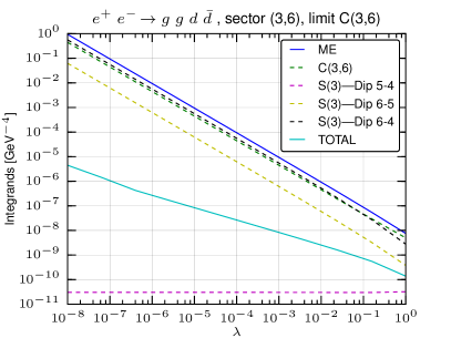
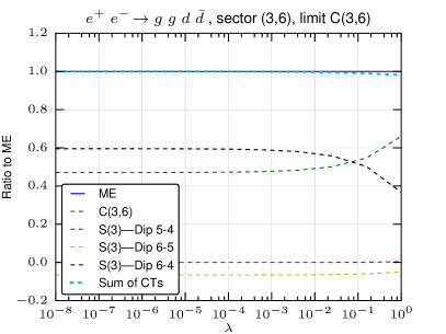
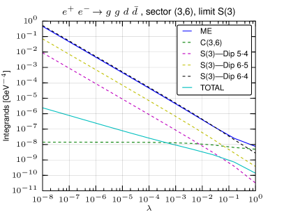
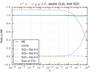
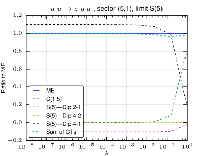
We start by showing in Figure 3 the case for $e^{+}e^{-}\to ggd\bar{d}$, and consider the sector identified by the first gluon and the $\bar{d}$ quark (labelled as 3, 6 in the particle list) both in case they become collinear (top row), and in case the gluon becomes soft (bottom row). Several quantities are displayed: the solid blue line represents the exact $({n+1})$-body matrix element, dubbed ME; thin dashed lines of different colours indicate the collinear counterterms C($x,y$), which include soft-collinear contributions, and the soft counterterms S($z$), split according to the different eikonal (or radiating dipole) contributions Dip $a$-$b$; the subtracted matrix element, labelled with TOTAL, is marked with a solid teal line, while the sum of all counterterms (Sum of CTs) is displayed with a thicker dashed line. Contributions are shown either in absolute value (left panels) or divided by the matrix element (right panels). Both sets of panels help conveying the message that the local cancellation of singularities has been achieved. In the left-hand plots, the $\lambda^{-1}$ slope of the real matrix element and of the counterterms is apparent, reducing to a $\lambda^{-1/2}$ behaviour for the subtracted result, which in turn becomes regular once combined with the phase-space measure. In the right plots one can appreciate how the various counterterms combine in such a way that their sum matches the matrix element in the relevant singular limit.

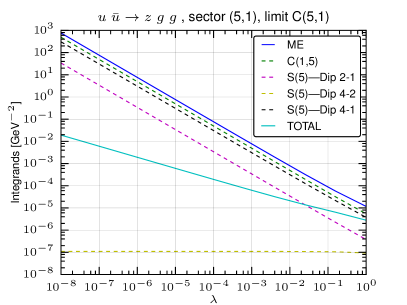
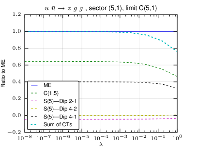
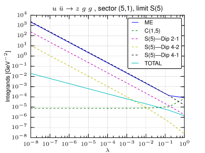
Turning to processes initiated by coloured particles, we show in Figure 4 the case for $u\bar{u}\to Zgg$ in the C(1,5) and S(5) configurations (i.e. those for which the last gluon (5) is collinear to the incoming $u$ quark (1), or soft), in the sector identified by particles 1, 5.

Figure 4: The singular behaviour of the real-emission matrix element and counterterms for the process $u\bar{u}\to Zgg$, in the sector identified by particles 1, 5. Top row: collinear configuration C(1,5); bottom row: soft configuration S(5).

Figure 5: The singular behaviour of the real-emission matrix element and counterterms for the process $dd\to ggdd$, in the sector identified by particles 1, 3. Top row: collinear configuration C(1,3); bottom row: soft configuration S(3).

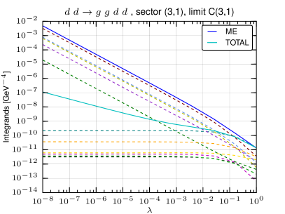
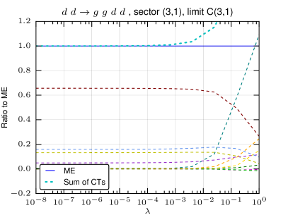
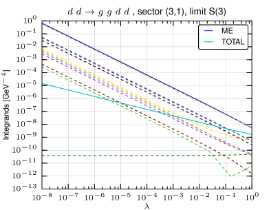
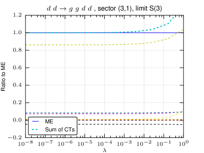
Analogously, in Figure 5, we consider the case of $dd\to ggdd$ in the C(1,3) and S(3) configurations, in the sector identified by particles 1, 3. Such a process has as many as 11 counterterms in this configuration (1 collinear and 10 soft dipoles), thus the displayed integrable scaling of the subtracted matrix element provides a highly non-trivial test of the correctness of the local subtraction mechanism.

5.2 Integrated results

We now turn to the numerical validation of our approach at the level of integrated cross sections for a selection of processes at NLO, comparing our results against those obtained with MadGraph5_aMC@NLO. The two main current limitations of our MadNkLO-based framework are the absence of a low-level code implementation, and of optimised phase-space integration routines. In fact, the integration is steered by a code written in Python, using Vegas3 Lepage:1980dq ; Lepage:2020tgj as integrator. Such a behaviour somewhat limits the complexity of the processes that can be run within a reasonable amount of time and computing resources; still, the processes we consider in the following cover all radiation topologies and both leptonic and hadronic collisions, hence we reckon them a sufficient subset for validation purposes.

The numerical setup we employ is the following: processes at lepton colliders are run at a centre-of-mass energy of 500 GeV. Hadronic processes are instead run at the LHC RunII energy of 13 TeV. In the latter case, the ${\rm PDF4LHC15\_nlo\_30}$ PDFs are employed Butterworth:2015oua , via the LHAPDF interface Buckley:2014ana . The fine-structure and Fermi constants have the values

$$\alpha=1/132.507,\qquad G_{f}=1.16639\cdot 10^{-5}\,\textrm{GeV}^{-2},$$ (87)

while the following values for particle masses are employed:

$$m_{Z}=91.188\,\textrm{GeV},\qquad m_{W}=80.419\,\textrm{GeV},\qquad m_{b}=4.7\,\textrm{GeV},\qquad m_{t}=173\,\textrm{GeV}.$$ (88)

Renormalisation and factorisation scales are kept fixed to $\mu=\mu_{F}=m_{Z}$.
Whenever light partons are present in the final state at the Born level, they are clustered into jets with the anti-$k_{t}$ algorithm Cacciari:2008gp , as implemented in FastJet Cacciari:2011ma , with radius parameter $R=0.4$. Jets are then required to satisfy the following kinematic cuts:

$$p_{T}(j)>20\,\textrm{GeV},\qquad|\eta(j)|<5.$$ (89)

The processes we consider are

$$e^{+}e^{-} \to jj,$$ (90)

$$e^{+}e^{-} \to jjj,$$ (91)

$$pp \to Z,$$ (92)

$$pp \to Zj,$$ (93)

$$pp \to W^{+}W^{-}j.$$ (94)

For these processes, we have computed the LO cross section and its NLO correction, which are quoted in Table 1. In this case, no damping factors are applied. Results from MadGraph5_aMC@NLO (dubbed aMC in the table) and MadNkLO are in general very well compatible, the largest deviations being of the order of the combined integration error, which is at or below the per-mille level.

Process	aMC LO	MadNkLO LO	aMC NLO corr.	MadNkLO NLO corr.
$e^{+}e^{-}\to jj$	0.53209(6)	0.53208(6)	0.019991(7)	0.019991(10)
$e^{+}e^{-}\to jjj$	0.4739(3)	0.4740(3)	-0.1461(1)	-0.1463(6)
$pp\to Z$	46361(3)	46362(3)	6810.9(8)	6810.8(4)
$pp\to Zj$	11270(7)	11258(5)	3770(6)	3776(17)
$pp\to W^{+}W^{-}j$	42.42(1)	42.39(2)	10.68(5)	10.53(13)

Table 1: Validation table with predictions for LO cross sections and NLO corrections. Numbers are in pb. Integration errors, on the last digit(s), are shown in parentheses.

We also consider the case of non-zero values for the damping parameters $\alpha,\beta,\gamma$ presented in Section 2.5. For simplicity, we set the three parameters to a common value, ranging from 0 to 2. Results for the NLO corrections are shown in Table 2, together with their breakdown into $n$-body and $({n+1})$-body contributions (the former including virtual corrections and integrated counterterms, the latter including subtracted real emissions). While the $n$- and $({n+1})$-body terms, if consider separately, show a very significant dependence upon the unphysical damping parameters, their sum remains stable, as expected. Results with the three different damping choices are totally compatible within the respective integration errors, and, in turn, with the MadGraph5_aMC@NLO results.

Process	MadNkLO	MadNkLO	MadNkLO
	$\alpha=\beta=\gamma=0$	$\alpha=\beta=\gamma=1$	$\alpha=\beta=\gamma=2$
$e^{+}e^{-}\to jj$
V+I	0.02664732(9)	0.01998531(7)	0.00666183(2)
R-K	-0.00666(1)	0.000004(6)	0.013329(6)
NLO corr.	0.019991(10)	0.019985(6)	0.019991(6)
$pp\to Z$
V+I+C+J	3981.5(4)	-3472.7(4)	-9163.2(5)
R-K	2829.3(2)	10284.3(4)	15974.1(6)
NLO corr.	6810.8(4)	6811.6(6)	6810.9(8)
$pp\to Zj$
V+I+C+J	7172(2)	5246(2)	3624(2)
R-K	-3395(17)	-1469(25)	156(22)
NLO corr.	3776(17)	3777(25)	3780(22)

Table 2: Validation table with predictions for the NLO corrections, broken down between $n$ and ${n+1}$ contributions, when different damping factors ($\alpha,\beta,\gamma$) are considered. Numbers are in pb. The integration error, on the last digit(s), is shown in parentheses.

5.3 Differential validation

Finally, we validate the correctness of the damping factors at the differential level in the simple case of $e^{+}e^{-}\to\gamma^{*}\to jj$, at centre-of-mass energy $\sqrt{s}=100$ GeV, with $\mu=35$ GeV. The plots in Figure 6 show differential cross sections with respect to transverse momentum and (absolute value of) pseudo-rapidity of the two hardest jets in the events (clustered with the $k_{t}$ algorithm Catani:1993hr ; Ellis:1993tq ), which are NLO-accurate observables receiving contribution from subtraction counterterms across the whole spectrum. A comparison is provided between predictions obtained with MadGraph5_aMC@NLO and an in-house implementation of local analytic sector subtraction, limited to the above-mentioned process. Various combinations of parameters $\alpha$ and $\beta$, ranging from 0 to 3, are chosen, in order to cover different damping possibilities ($\gamma$ is irrelevant for final-state radiation).

Figure 6: Transverse momenta and pseudo-rapidities for the two hardest jets in $e^{+}e^{-}\to\gamma^{*}\to jj$ at NLO, comparing aMC and local analytic sector subtraction.

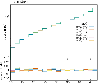
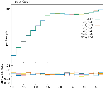
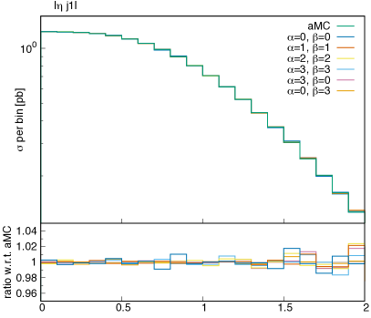
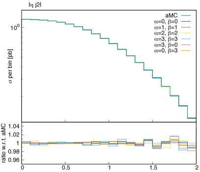
As evident from Figure 6, predictions of local analytic sector subtraction for all chosen damping profiles are in excellent agreement with those obtained with aMC within the numerical accuracy used for the runs. A systematic study of the performance of the various damping choices at the differential level in more complex processes and setups is however beyond the scope of this paper, and postponed to future work.

6 Conclusion

We have presented the extension of the local analytic sector subtraction method to the case of initial-state QCD radiation at NLO. We have shown that the enhanced structural simplicity of the method, already evident in the case of final-state radiation, carries over to initial-state radiation, which represents a promising feature with a view to NNLO subtraction for hadron-collider processes.

Aiming at an improved numerical stability, we have introduced an optimisation procedure to tune the impact of subtraction terms in the non-singular regions of phase space, in a way that preserves the properties of the method, in particular the simplicity of the involved analytic integrations.

Finally, we have presented the first implementation of the method in an automated framework, MadNkLO, and validated its correctness at the level of singular infrared and collinear limits and, mainly, of physical cross sections, for a set of simple collider processes involving initial- and final-state radiation.

The natural directions to be followed after this work are on one hand a systematic optimisation of the numerical software, necessary to reduce the time and CPU resources necessary to produce phenomenological results; on the other hand, the inclusion of a subtraction scheme for massive final-state particles at NLO, relevant for top- and bottom-quark physics, and, most importantly, the definition of local analytic sector subtraction for initial-state radiation at NNLO.

Appendix A Altarelli-Parisi splitting kernels

We collect here the expression for the regularised Altarelli-Parisi collinear kernels appearing in the lowest-order DGLAP Gribov:1972ri ; Altarelli:1977zs ; Dokshitzer:1977sg evolution equations.

$$\bar{P}_{a}(x)\,B \equiv \delta_{f_{a}g}\Big{[}\bar{P}_{gg}(x)\,B^{(g)}+\bar{P}_{q\bar{q}}(x)\,\big{(}B^{(q)}+B^{(\bar{q})}\big{)}\Big{]}$$ (95)

$$+\,\delta_{f_{a}\{q,\bar{q}\}}\Big{[}\bar{P}_{gq}(x)\,B^{(g)}+\bar{P}_{qg}(x)\,B^{(f_{a})}\Big{]}\,,$$

where

$$\bar{P}_{gg}(x) = 2\,C_{A}\left[\frac{x}{(1-x)_{+}}\!+\frac{1-x}{x}+x(1-x)\right]+\delta(1-x)\,\frac{\beta_{0}}{2}\,,$$

$$\bar{P}_{q\bar{q}}(x) = T_{R}\left[x^{2}+(1-x)^{2}\right]\,,$$

$$\bar{P}_{qg}(x) = C_{F}\left(\frac{1+x^{2}}{1-x}\right)_{\!\!+}\!\,,$$

$$\bar{P}_{gq}(x) = C_{F}\,\frac{1+(1-x)^{2}}{x}\,,$$ (96)

$C_{A}=N_{c}$, $C_{F}=(N_{c}^{2}-1)/(2N_{c})$, $T_{R}=1/2$, $\beta_{0}=(11\,C_{A}-4\,T_{R}\,N_{f})/3$, and $B^{(f_{i})}$ denotes the Born contribution initiated by a parton of flavour $f_{i}$, stemming from the splitting of parton $a$.

We also collect here finite terms arising from the integration of initial-state collinear counterterms, see Sections 4.2, 4.3, which are related to the Altarelli-Parisi kernels:

$$P_{a,\text{fin}}^{(\lambda)}(x)\,B \equiv \delta_{f_{a}g}\Big{[}p^{(\lambda)}_{gg}(x)\,B^{(g)}+p^{(\lambda)}_{q\bar{q}}(x)\,\big{(}B^{(q)}+B^{(\bar{q})}\big{)}\Big{]}$$ (97)

$$+\,\delta_{f_{a}\{q,\bar{q}\}}\Big{[}p^{(\lambda)}_{gq}(x)\,B^{(g)}+p^{(\lambda)}_{qg}(x)\,B^{(f_{a})}\Big{]}\,,\qquad$$

where $\lambda=1,2$,

$$p^{(\lambda)}_{gg}(x) = 2\,C_{A}\left(\frac{1-x}{x}+x(1-x)\right)\Big{[}\lambda\,\ln(1-x)-A_{1}(\gamma)\Big{]}\,,$$

$$p^{(\lambda)}_{q\bar{q}}(x) = T_{R}\left(x^{2}+(1-x)^{2}\right)\Big{[}\lambda\,\ln(1-x)-A_{1}(\gamma)\Big{]}+T_{R}\,2x\,(1-x)\,,$$

$$p^{(\lambda)}_{qg}(x) = C_{F}\,(1-x)\Big{[}\lambda\,\ln(1-x)+1-A_{1}(\gamma)\Big{]}\,,$$

$$p^{(\lambda)}_{gq}(x) = C_{F}\,\frac{1+(1-x)^{2}}{x}\Big{[}\lambda\,\ln(1-x)-A_{1}(\gamma)\Big{]}+C_{F}\,x\,,$$ (98)

and $A_{1}(\gamma)$ is defined in Appendix D.

Appendix B Phase-space mappings

In this appendix we report the phase-space mappings and parametrisations, used throughout the main text, for initial- and final-state radiation. These mappings are taken from Catani-Seymour dipole subtraction Catani:1996vz .

B.1 Final $a,b,c$

The first configuration we study is shown in leftmost panel of Figure 2. Remapped momenta are defined as

$$\bar{k}^{(abc)}_{b}\,=\,k_{a}+k_{b}-\frac{y}{1-y}\,k_{c}\,,\quad\quad\bar{k}^{(abc)}_{c}\,=\,\frac{1}{1-y}\,k_{c}\,,\quad\quad\bar{k}^{(abc)}_{i}\,=\,k_{i}\,,\,\forall i\,\neq\,(a,b,c)\,,$$ (99)

as functions of the Catani-Seymour variables $0\leq y,z\leq 1$

$$y\,=\,\frac{s_{ab}}{s_{abc}}\ ,\quad\quad\quad z\,=\,\frac{s_{ac}}{s_{ac}+s_{bc}}\ .$$ (100)

Given the dipole centre-of-mass squared energy $\bar{s}_{bc}^{(abc)}\equiv 2\bar{k}_{b}^{(abc)}\cdot\bar{k}_{c}^{(abc)}$, the Mandelstam invariants satisfy the following relations:

$$s_{ab}\,=\,y\,\bar{s}_{bc}^{(abc)}\,,\qquad s_{ac}\,=\,z(1-y)\,\bar{s}_{bc}^{(abc)}\,,\qquad s_{bc}\,=\,(1-z)(1-y)\,\bar{s}_{bc}^{(abc)}\,.$$ (101)

The remapping allows to factorise the radiative phase space from the $n$-body phase space as

$$\int d\Phi_{n+1}\,=\,\frac{\varsigma_{n+1}}{\varsigma_{n}}\int d\Phi_{n}^{(abc)}\int d\Phi_{\rm rad}^{(abc)}\,,$$ (102)

where $\varsigma_{m}$ is the multiplicity factor for the $m$-body phase space and

$$d\Phi_{n}^{(abc)}\,\equiv\,d\Phi_{n}\left(\{\bar{k}\}^{(abc)}\right)\,,\qquad d\Phi_{\rm rad}^{(abc)}\,\equiv\,d\Phi_{\rm rad}\Big{(}\bar{s}_{bc}^{(abc)};y,z,\phi\Big{)}\,,$$ (103)

$$\int d\Phi_{\rm rad}^{(abc)}\,=\,N(\epsilon)\left(\bar{s}_{bc}^{(abc)}\right)^{1-\epsilon}\!\int_{0}^{\pi}\!\!d\phi\,\sin^{-2\epsilon}\!\phi\int_{0}^{1}\!\!dy\int_{0}^{1}\!\!dz\Big{[}y(1-y)^{2}\,z(1-z)\Big{]}^{-\epsilon}\!(1-y)\,,$$ (104)

with

$$N(\epsilon)\,\equiv\,\frac{(4\pi)^{\epsilon-2}}{\sqrt{\pi}\,\Gamma(1/2-\epsilon)}\,.$$ (105)

B.2 Final $a,b$, initial $c$

Considering the central panel of Figure(2), we choose to boost the incoming momentum, i.e.

$$\bar{k}^{(abc)}_{b}\,=\,k_{a}+k_{b}-(1-x)\,k_{c}\,,\quad\quad\bar{k}^{(abc)}_{c}\,=\,x\,k_{c}\,,\quad\quad\bar{k}^{(abc)}_{i}\,=\,k_{i}\,,\,\forall i\,\neq\,(a,b,c)\,,$$ (106)

where we introduced kinematic variables $0\leq x,z\leq 1$ defined as

$$x\,=\,\frac{s_{ac}+s_{bc}-s_{ab}}{s_{ac}+s_{bc}}\,,\qquad z\,=\,\frac{s_{ac}}{s_{ac}+s_{bc}}\,.$$ (107)

As a function of the reference invariant $\bar{s}_{bc}^{(abc)}=2\bar{k}_{b}^{(abc)}\cdot k_{c}=2\bar{k}_{b}^{(abc)}\cdot\bar{k}_{c}^{(abc)}/x$, the dot products are

$$s_{ab}\,=\,(1-x)\ \bar{s}_{bc}^{(abc)}\,,\qquad s_{ac}\,=\,z\,\bar{s}_{bc}^{(abc)}\,,\qquad s_{bc}\,=\,(1-z)\,\bar{s}_{bc}^{(abc)}\,.$$ (108)

In this case the radiative phase space cannot be exactly factorised as in Eq. (102) due to the dependence of the reference scale $\bar{s}_{bc}^{(abc)}$ upon the variable $x$ associated to the rescaled momentum of the initial-state parton, over which we are not integrating. Thus we define the following convolution,

$$\int d\Phi_{n+1}(k_{c})\,=\,\frac{\varsigma_{n+1}}{\varsigma_{n}}\int\int d\Phi_{n}^{(abc)}(xk_{c})\,d\Phi_{\rm rad}^{(abc)}\,,$$ (109)

with

$$d\Phi_{n}^{(abc)}\!(xk_{c})\,\equiv\,d\Phi_{n}\left(\{\bar{k}\}^{(abc)}\right)\,,\qquad d\Phi_{\rm rad}^{(abc)}\,\equiv\,d\Phi_{\rm rad}\Big{(}\bar{s}_{bc}^{(abc)};x,z,\phi\Big{)}\,.$$ (110)

The single unresolved phase space in terms of the kinematic variables reads

$$\int d\Phi_{\rm rad}^{(abc)}\,=\,N(\epsilon)\left(\bar{s}_{bc}^{(abc)}\right)^{1-\epsilon}\int_{0}^{\pi}\!\!d\phi\,\sin^{-2\epsilon}\!\phi\int_{0}^{1}\!\!dx\int_{0}^{1}\!\!dz\,[(1-x)\,z(1-z)]^{-\epsilon}\,.$$ (111)

B.3 Final $a$, initial $b,c$

In the counterterms featuring two incoming partons, we set the incoming momentum $\bar{k}_{b}$ to be parallel to $k_{b}$ while leaving unchanged the other incoming momentum, $\bar{k}^{\mu}_{c}=k^{\mu}_{c}$. Then we shift all other final-state momenta collected in $k_{f}=\{k_{j}\}_{j\in\rm F}$, as

$$\bar{k}^{(abc)}_{b} = x\,k_{b}\,,\quad\quad\quad\bar{k}^{(abc)}_{c}\,=\,k_{c}\,,$$

$$\bar{k}^{(abc)}_{f} = k_{f}-\frac{2k_{f}\cdot(K+\widebar{K})}{(K+\widebar{K})^{2}}\,(K+\widebar{K})+\frac{2k_{f}\cdot K}{K^{2}}\,\widebar{K}\,,\qquad\forall f\,\neq\,(a,b,c)\,,$$ (112)

with

$$K\,=\,k_{b}+k_{c}-k_{a}\,,\quad\quad\quad\widebar{K}\,=\,\bar{k}_{b}^{(abc)}+\bar{k}_{c}^{(abc)}\,.$$ (113)

The kinematic variables adopted in this case, satisfying $0\leq x,v\leq 1$, are

$$x\,=\,\frac{s_{bc}-s_{ab}-s_{ac}}{s_{bc}}\,,\qquad v\,=\,\frac{s_{ab}}{s_{ab}+s_{ac}}\,,$$ (114)

and with respect to the invariant $\bar{s}_{bc}^{(abc)}=2k_{b}\cdot k_{c}=2\bar{k}_{b}^{(abc)}\cdot\bar{k}_{c}^{(abc)}/x$ we rewrite the dipole Mandelstam invariants as

$$s_{ab}\,=\,(1-x)\,v\,\bar{s}_{bc}^{(abc)}\,,\qquad s_{ac}\,=\,(1-x)\,(1-v)\,\bar{s}_{bc}^{(abc)}\,,\qquad s_{bc}\,=\,\bar{s}_{bc}^{(abc)}\,.$$ (115)

Then we parametrise the $({n+1})$-body phase space as a convolution over $x$ of $d\Phi_{n}$ and $d\Phi_{\rm rad}$ as

$$\int d\Phi_{n+1}(k_{b},k_{c})\,=\,\frac{\varsigma_{n+1}}{\varsigma_{n}}\int\int d\Phi_{n}^{(abc)}(xk_{b},k_{c})\,d\Phi_{\rm rad}^{(abc)}\,,$$ (116)

with

$$d\Phi_{n}^{(abc)}(xk_{b},k_{c})\,\equiv\,d\Phi_{n}\left(\{\bar{k}\}^{(abc)}\right)\,,\qquad d\Phi_{\rm rad}^{(abc)}\,\equiv\,d\Phi_{\rm rad}\Big{(}\bar{s}_{bc}^{(abc)};x,v,\phi\Big{)}\,,$$ (117)

leading to the explicit expression

$$\int d\Phi_{\rm rad}^{(abc)}\,=\,N(\epsilon)\left(\bar{s}_{bc}^{(abc)}\right)^{1-\epsilon}\int_{0}^{\pi}\!\!d\phi\,\sin^{-2\epsilon}\!\phi\int_{0}^{1}\!\!dx\int_{0}^{1}\!\!dv\,[(1-x)^{2}\,v(1-v)]^{-\epsilon}(1-x)\,.$$ (118)

Appendix C Consistency relations

In this Section we explicitly verify the relations in Eqs. (2.4) for initial- and final-state radiation, ensuring the locality of the subtraction procedure.

As far as relation ${\bf S}_{i}\,\overline{\bf S}_{i}\,R\,=\,{\bf S}_{i}\,R$ is concerned, this is trivially verified since ${\bf S}_{i}\,\{\bar{k}\}^{(ikl)}={\bf S}_{i}\,\{\bar{k}\}^{(ilk)}=\{k\}_{\not{i}}$ for soft emission from both the initial and the final state, hence

$${\bf S}_{i}\,\overline{\bf S}_{i}\,R = -\mathcal{N}_{1}\,\sum_{k\neq i}\sum_{l\neq i}\,\mathcal{I}^{(i)}_{kl}\ B_{kl}(\{k\}_{\not{i}})\,=\,{\bf S}_{i}\,R\,.$$ (119)

Analogously, for the collinear relation ${\bf C}_{ij}\,\overline{\bf C}_{ij}\,R\,=\,{\bf C}_{ij}\,R$, the key ingredients are the limits

$${\bf C}_{ij}\,x\,\theta_{{i}\in{\rm F}}\,\theta_{{j}\in{\rm I}}\,=\,x_{[ij]}\,\theta_{{i}\in{\rm F}}\,\theta_{{j}\in{\rm I}}\,,$$ (120)

as well as

$${\bf C}_{ij}\,\{\bar{k}\}^{(ijr)}\,\theta_{{i}\in{\rm F}}\,\theta_{{j}\in{\rm F}} = \big{(}\{k\}_{\not{i}\not{j}},k_{[ij]}\big{)}\,\theta_{{i}\in{\rm F}}\,\theta_{{j}\in{\rm F}}\,,$$

$${\bf C}_{ij}\,\{\bar{k}\}^{(ijr)}\,\theta_{{i}\in{\rm F}}\,\theta_{{j}\in{\rm I}}\,\theta_{{r}\in{\rm I}} = {\bf C}_{ij}\,\{\bar{k}\}^{(irj)}\,\theta_{{i}\in{\rm F}}\,\theta_{{j}\in{\rm I}}\,\theta_{{r}\in{\rm F}}\,=\,\big{(}\{k\}_{\not{i}\not{j}},x_{[ij]}\,k_{j}\big{)}\,\theta_{{i}\in{\rm F}}\,\theta_{{j}\in{\rm I}}\,,$$ (121)

from which one immediately deduces

$${\bf C}_{ij}\,\overline{\bf C}_{ij}\,R = \frac{\mathcal{N}_{1}}{s_{ij}}\,\Bigg{[}\theta_{{i}\in{\rm F}}\,\theta_{{j}\in{\rm F}}\,P_{ij,\rm F}^{\mu\nu}(z_{i})\,B_{\mu\nu}\!\left(\{k\}_{\not{i}\not{j}},k_{[ij]}\right)$$ (122)

$$\qquad+\,\theta_{{i}\in{\rm F}}\,\theta_{{j}\in{\rm I}}\,\frac{P_{[ij]i,\rm I}^{\mu\nu}(x_{[ij]})}{x_{[ij]}}\,B_{\mu\nu}\!\left(\{k\}_{\not{i}\not{j}},x_{[ij]}k_{j}\right)$$

$$\qquad+\,\theta_{{j}\in{\rm F}}\,\theta_{{i}\in{\rm I}}\,\frac{P_{[ji]j,\rm I}^{\mu\nu}(x_{[ji]})}{x_{[ji]}}\,B_{\mu\nu}\!\left(\{k\}_{\not{i}\not{j}},x_{[ji]}k_{i}\right)\Bigg{]}\,=\,{\bf C}_{ij}\,R\,.$$

Moving on to relation ${\bf S}_{i}\,\overline{\bf S}_{i}\,\overline{\bf C}_{ij}\,R\,=\,{\bf S}_{i}\,\overline{\bf C}_{ij}\,R$, this is a consequence of the fact that

$${\bf S}_{i}\,\overline{\bf S}_{i}\,\overline{\bf C}_{ij}\,R\,=\,\,\mathcal{N}_{1}\,\delta_{f_{i}g}\,2\,C_{f_{j}}\,\frac{s_{jr}}{s_{ij}\,\big{(}s_{ir}+\theta_{{j}\in{\rm I}}\,\theta_{{r}\in{\rm I}}\,s_{ij}\big{)}}\,B\Big{(}\{k\}_{\not{i}}\Big{)}\,=\,{\bf S}_{i}\,\overline{\bf C}_{ij}\,R\,,$$ (123)

having explicitly employed the soft behaviour of Altarelli-Parisi kernels.

The final relation ${\bf C}_{ij}\,\overline{\bf S}_{i}\,\overline{\bf C}_{ij}\,R\,=\,{\bf C}_{ij}\,\overline{\bf S}_{i}\,R$ is instead slightly subtler. The explicit collinear action on the soft counterterm is

$${\bf C}_{ij}\,\overline{\bf S}_{i}\,R = -\,2\,\mathcal{N}_{1}\,\mathcal{I}_{jr}^{(i)}\,{\bf C}_{ij}\bigg{\{}\sum_{\begin{subarray}{c}k\neq i\\ k<j\end{subarray}}\Big{[}\big{(}\theta_{{j}\in{\rm I}}\,\theta_{{k}\in{\rm I}}\!+\!\theta_{{j}\in{\rm F}}\,\theta_{{k}\in{\rm I}}\!+\!\theta_{{j}\in{\rm F}}\,\theta_{{k}\in{\rm F}}\big{)}\bar{B}^{(ijk)}_{jk}\!+\theta_{{j}\in{\rm I}}\,\theta_{{k}\in{\rm F}}\,\bar{B}^{(ikj)}_{jk}\Big{]}$$ (124)

$$\hskip 65.44133pt+\sum_{\begin{subarray}{c}k\neq i\\ k>j\end{subarray}}\Big{[}\big{(}\theta_{{k}\in{\rm I}}\,\theta_{{j}\in{\rm I}}\!+\!\theta_{{k}\in{\rm F}}\,\theta_{{j}\in{\rm I}}\!+\!\theta_{{k}\in{\rm F}}\,\theta_{{j}\in{\rm F}}\big{)}\bar{B}^{(ikj)}_{jk}\!+\theta_{{k}\in{\rm I}}\,\theta_{{j}\in{\rm F}}\,\bar{B}^{(ijk)}_{jk}\Big{]}\bigg{\}}$$

$$= -\,2\,\mathcal{N}_{1}\,\mathcal{I}_{jr}^{(i)}\,{\bf C}_{ij}\,\bigg{\{}\sum_{\begin{subarray}{c}k\neq i\\ k<j\end{subarray}}\Big{[}\big{(}\theta_{{j}\in{\rm I}}\,\theta_{{k}\in{\rm I}}+\theta_{{j}\in{\rm F}}\,\theta_{{k}\in{\rm F}}\big{)}\,\bar{B}^{(ijk)}_{jk}\Big{]}$$

$$\hskip 68.2866pt+\sum_{\begin{subarray}{c}k\neq i\\ k>j\end{subarray}}\Big{[}\big{(}\theta_{{j}\in{\rm I}}\,\theta_{{k}\in{\rm I}}+\theta_{{j}\in{\rm F}}\,\theta_{{k}\in{\rm F}}\big{)}\,\bar{B}^{(ikj)}_{jk}\Big{]}$$

$$\hskip 68.2866pt+\sum_{\begin{subarray}{c}k\neq i,j\end{subarray}}\Big{[}\theta_{{j}\in{\rm F}}\,\theta_{{k}\in{\rm I}}\,\bar{B}^{(ijk)}_{jk}+\theta_{{j}\in{\rm I}}\,\theta_{{k}\in{\rm F}}\,\bar{B}^{(ikj)}_{jk}\Big{]}\bigg{\}}\,,\qquad$$

where we have used that ${\bf C}_{ij}\,\mathcal{I}^{(i)}_{jk}=\mathcal{I}^{(i)}_{jr}$ is independent of $k$, and can be taken out of the sum. The action of ${\bf C}_{ij}$ on the mapped Born kinematics reads

$${\bf C}_{ij}\,\theta_{{j}\in{\rm F}}\,\theta_{{k}\in{\rm F}}\,\bar{B}^{(ijk)}_{jk}={\bf C}_{ij}\,\theta_{{j}\in{\rm F}}\,\theta_{{k}\in{\rm F}}\,\bar{B}^{(ikj)}_{jk}=\theta_{{j}\in{\rm F}}\,\theta_{{k}\in{\rm F}}\,B_{jk}\Big{(}\{k\}_{\not{i}\not{j}},k_{[ij]}\Big{)}\,,$$

$${\bf C}_{ij}\,\theta_{{j}\in{\rm F}}\,\theta_{{k}\in{\rm I}}\,\bar{B}^{(ijk)}_{jk}=\theta_{{j}\in{\rm F}}\,\theta_{{k}\in{\rm I}}\,B_{jk}\Big{(}\{k\}_{\not{i}\not{j}},k_{[ij]}\Big{)}\,,$$

$${\bf C}_{ij}\,\theta_{{j}\in{\rm I}}\,\theta_{{k}\in{\rm F}}\,\bar{B}^{(ikj)}_{jk}=\theta_{{j}\in{\rm I}}\,\theta_{{k}\in{\rm F}}\,B_{jk}\Big{(}\{k\}_{\not{i}\not{j}},x_{[ij]}k_{j}\Big{)}\,,$$

$${\bf C}_{ij}\,\theta_{{j}\in{\rm I}}\,\theta_{{k}\in{\rm I}}\,\bar{B}^{(ijk)}_{jk}={\bf C}_{ij}\,\theta_{{j}\in{\rm I}}\,\theta_{{k}\in{\rm I}}\,\bar{B}^{(ikj)}_{jk}=\theta_{{j}\in{\rm I}}\,\theta_{{k}\in{\rm I}}\,B_{jk}\Big{(}\{k\}_{\not{i}\not{j}},x_{[ij]}k_{j}\Big{)}\,,$$ (125)

where the latter equality is proven in Appendix C.1. At this point, one can recast Eq. (124) as

$${\bf C}_{ij}\,\overline{\bf S}_{i}\,R = -\,2\,\mathcal{N}_{1}\,\mathcal{I}_{jr}^{(i)}\,\sum_{\begin{subarray}{c}k\neq i,j\end{subarray}}\bigg{[}\theta_{{j}\in{\rm I}}\,B_{jk}\Big{(}\{k\}_{\not{i}\not{j}},x_{[ij]}k_{j}\Big{)}+\theta_{{j}\in{\rm F}}\,B_{jk}\Big{(}\{k\}_{\not{i}\not{j}},k_{[ij]}\Big{)}\bigg{]}\,.$$ (126)

Upon enforcing colour conservation, $\sum_{k\neq j}{\bf T}_{k}=-{\bf T}_{j}$, this becomes

$${\bf C}_{ij}\,\overline{\bf S}_{i}\,R = 2\,\mathcal{N}_{1}\,C_{f_{j}}\,\mathcal{I}^{(i)}_{jr}\,\bigg{[}\theta_{{j}\in{\rm I}}\,B\Big{(}\{k\}_{\not{i}\not{j}},x_{[ij]}k_{j}\Big{)}+\theta_{{j}\in{\rm F}}\,B\Big{(}\{k\}_{\not{i}\not{j}},k_{[ij]}\Big{)}\bigg{]}\,.$$ (127)

Recalling that ${\bf C}_{ij}\,z^{(irj)}\,\theta_{{j}\in{\rm I}}\,\theta_{{r}\in{\rm F}}={\bf C}_{ij}\,v^{(ijr)}\,\theta_{{j}\in{\rm I}}\,\theta_{{r}\in{\rm I}}=0$, it is straightforward at this point to verify that the espression in Eq. (124) matches the result of ${\bf C}_{ij}\,\overline{\bf S}_{i}\,\overline{\bf C}_{ij}\,R$ for all choices of remapping, showing the consistency relation.

C.1 Collinear limits on mappings with two initial-state partons

In this Appendix we show the last of Eqs. (C), namely that, under the collinear ${\bf C}_{ij}$ limit, both $\theta_{{j}\in{\rm I}}\,\theta_{{k}\in{\rm I}}\,\bar{B}^{(ijk)}_{jk}$ and $\theta_{{j}\in{\rm I}}\,\theta_{{k}\in{\rm I}}\,\bar{B}^{(ikj)}_{jk}$ tend to $\theta_{{j}\in{\rm I}}\,\theta_{{k}\in{\rm I}}\,B_{jk}\Big{(}\{k\}_{\not{i}\not{j}},x_{[ij]}k_{j}\Big{)}$. The proof is based on the fact that, although the two sets of momenta do not match in the limit, the colour- (as opposed to spin-) connected Born squared amplitudes depend on kinematics only through Mandelstam invariants, which do coincide in the ${\bf C}_{ij}$ limit, as shown below.

Considering particles $j$ and $k$ in the initial state, while $i$ and $f$ in the final state, we analyse the ${\bf C}_{ij}$ limit for the mappings $(ijk)$ and $(ikj)$.

• Mapping $(ijk)$

  $$\bar{k}_{j} = x\,k_{j}\,,$$ (128)

  $$\bar{k}_{k} = k_{k}\,,$$

  $$\bar{k}_{f} = k_{f}-\frac{2k_{f}\cdot(K+\widebar{K}_{(1)})}{(K+\widebar{K}_{(1)})^{2}}\,(K+\widebar{K}_{(1)})+\frac{2k_{f}\cdot K}{(K)^{2}}\,\widebar{K}_{(1)}\,,$$

  with

  $$x=\frac{s_{jk}-s_{ij}-s_{ik}}{s_{jk}}\,,\qquad K=k_{j}+k_{k}-k_{i}\,,\qquad\widebar{K}_{(1)}=\bar{k}_{j}+\bar{k}_{k}=xk_{j}+k_{k}\,.\qquad$$ (129)

  Under ${\bf C}_{ij}$ collinear limit, denoting with $E_{a}$ the energy of parton $a$ in arbitrary frame, and with $r$ the ratio $E_{i}/E_{j}$, one has

  $$s_{ij}\,\xrightarrow{{\bf C}_{ij}}\,0\,,\qquad s_{ik}\,\xrightarrow{{\bf C}_{ij}}\,s_{jk}\,r\,,\qquad s_{if}\,\xrightarrow{{\bf C}_{ij}}\,s_{jf}\,r\,,$$ (130)

  $$x\,\xrightarrow{{\bf C}_{ij}}\,1-r\,,\qquad K\,\xrightarrow{{\bf C}_{ij}}\,k_{j}(1-r)+k_{k}\,,\qquad\widebar{K}_{(1)}\,\xrightarrow{{\bf C}_{ij}}\,k_{j}(1-r)+k_{k}\,,$$

  $$2\,\bar{k}_{j}\cdot\bar{k}_{f}\,\xrightarrow{{\bf C}_{ij}}\,s_{jf}\,(1-r)\,,\qquad 2\,\bar{k}_{k}\cdot\bar{k}_{f}\,\xrightarrow{{\bf C}_{ij}}\,s_{kf}\,,\qquad 2\,\bar{k}_{j}\cdot\bar{k}_{k}\,\xrightarrow{{\bf C}_{ij}}\,s_{jk}\,(1-r)\,.$$

• Mapping $(ikj)$

  $$\bar{k}_{j} = k_{j}\,,$$ (131)

  $$\bar{k}_{k} = x\,k_{k}\,,$$

  $$\bar{k}_{f} = k_{f}-\frac{2k_{f}\cdot(K+\widebar{K}_{(2)})}{(K+\widebar{K}_{(2)})^{2}}\,(K+\widebar{K}_{(2)})+\frac{2k_{f}\cdot K}{(K)^{2}}\,\widebar{K}_{(2)}\,,$$

  with

  $$x=\frac{s_{jk}-s_{ij}-s_{ik}}{s_{jk}}\,,\qquad K=k_{j}+k_{k}-k_{i}\,,\qquad\widebar{K}_{(2)}=\bar{k}_{j}+\bar{k}_{k}=k_{j}+xk_{k}\,.\qquad$$ (132)

  Under ${\bf C}_{ij}$ collinear limit, denoting with $E_{a}$ the energy of parton $a$ in arbitrary frame, and with $r$ the ratio $E_{i}/E_{j}$, one has

  $$s_{ij}\,\xrightarrow{{\bf C}_{ij}}\,0\,,\qquad s_{ik}\,\xrightarrow{{\bf C}_{ij}}\,s_{jk}\,r\,,\qquad s_{if}\,\xrightarrow{{\bf C}_{ij}}\,s_{jf}\,r\,,$$ (133)

  $$x\,\xrightarrow{{\bf C}_{ij}}\,1-r\,,\qquad K\,\xrightarrow{{\bf C}_{ij}}\,k_{j}(1-r)+k_{k}\,,\qquad\widebar{K}_{(2)}\,\xrightarrow{{\bf C}_{ij}}\,k_{j}+k_{k}(1-r)\,,$$

  $$2\,\bar{k}_{j}\cdot\bar{k}_{f}\,\xrightarrow{{\bf C}_{ij}}\,s_{jf}\,(1-r)\,,\qquad 2\,\bar{k}_{k}\cdot\bar{k}_{f}\,\xrightarrow{{\bf C}_{ij}}\,s_{kf}\,,\qquad 2\,\bar{k}_{j}\cdot\bar{k}_{k}\,\xrightarrow{{\bf C}_{ij}}\,s_{jk}\,(1-r)\,.$$

Invariants built with the two different remappings are identical in the collinear ${\bf C}_{ij}$ limit. The proof of the last of Eq. (C) is completed by the fact that ${\bf C}_{ij}\,x\,=\,{\bf C}_{ij}\,x_{[ij]}\,=\,1-r$.

Appendix D Library of integrals

The analytical results collected in this Section depend on the following functions

$$A_{1}(\xi) \equiv \gamma_{E}+\Psi^{(0)}(\xi+1)\,,$$

$$A_{2}(\xi) \equiv \gamma_{E}-1+\Psi^{(0)}(\xi+2)\,=\,A_{1}(\xi+1)-1\,,$$

$$A_{3}(\xi) \equiv 1-\zeta_{2}+\Psi^{(1)}(\xi+2)\,,$$ (134)

where $\xi\geq 0$, $\gamma_{E}=0.5772156649...$ is the Euler-Mascheroni constant, $\Psi^{(n)}(z)$ is the $n$-th Polygamma function, namely

$$\Psi^{(n)}(z)=\frac{d^{{n+1}}}{dz^{{n+1}}}\,\ln[\Gamma(z)]\,,$$ (135)

and all functions $A_{i}(\xi)$ satisfy $A_{i}(0)=0$.

D.1 Soft counterterms

For $\star\star$ taking value in $\rm F\rm F,\rm F\rm I,\rm I\rm I$, we define

$$I_{\rm s,\star\star}^{abc} \equiv \delta_{f_{a}g}\,I_{\rm s,\star\star}\big{(}\bar{s}_{bc}^{(abc)}\big{)}\,,$$ (136)

$$J_{\rm s,\star\star}^{abc}(x) \equiv \delta_{f_{a}g}\,J_{\rm s,\star\star}\big{(}\bar{s}_{bc}^{(abc)},x\big{)}\,,$$ (137)

where the relevant integrals obtained integrating the soft counterterm in Eq. (63) read

$$I_{\rm s,\rm F\rm F}(s) = \frac{\alpha_{\mbox{\tiny{S}}}}{2\pi}\left(\frac{s}{e^{\gamma_{\!{}_{{}_{E}}}\!}\mu^{2}}\right)^{\!\!-\epsilon}\frac{\Gamma(1-\epsilon)\Gamma(2+\alpha-\epsilon)}{\epsilon^{2}\,\Gamma(2+\alpha-3\epsilon)}$$

$$= \frac{\alpha_{\mbox{\tiny{S}}}}{2\pi}\left(\frac{s}{\mu^{2}}\right)^{\!\!-\epsilon}\bigg{[}\frac{1}{\epsilon^{2}}+\frac{2}{\epsilon}-\frac{7\pi^{2}}{12}+6+2\,A_{2}(\alpha)\bigg{(}\frac{1}{\epsilon}+2+A_{2}(\alpha)\bigg{)}-4\,A_{3}(\alpha)+\mathcal{O}(\epsilon)\bigg{]}\,,$$

$$I_{\rm s,\rm F\rm I}(s) = \frac{\alpha_{\mbox{\tiny{S}}}}{2\pi}\left(\frac{s}{e^{\gamma_{\!{}_{{}_{E}}}\!}\mu^{2}}\right)^{\!\!-\epsilon}\frac{\Gamma(1-\epsilon)\,\Gamma(2+\alpha)}{\epsilon^{2}\,\Gamma(2+\alpha-2\epsilon)}$$

$$= \frac{\alpha_{\mbox{\tiny{S}}}}{2\pi}\left(\frac{s}{\mu^{2}}\right)^{\!\!-\epsilon}\bigg{[}\frac{1}{\epsilon^{2}}+\frac{2}{\epsilon}-\frac{\pi^{2}}{4}+4+2\,A_{2}(\alpha)\bigg{(}\frac{1}{\epsilon}+2+A_{2}(\alpha)\bigg{)}-2\,A_{3}(\alpha)+\mathcal{O}(\epsilon)\bigg{]}\,,$$

$$I_{\rm s,\rm I\rm I}(s) = \frac{\alpha_{\mbox{\tiny{S}}}}{2\pi}\left(\frac{s}{e^{\gamma_{\!{}_{{}_{E}}}\!}\mu^{2}}\right)^{\!\!-\epsilon}\frac{\Gamma(1-\epsilon)\,\Gamma(2+\alpha)}{\epsilon^{2}\,\Gamma(2+\alpha-2\epsilon)}\,=\,I_{\rm s,\rm F\rm I}(s)\,;$$ (140)

$$J_{\rm s,\rm F\rm I}(s,x) = \frac{\alpha_{\mbox{\tiny{S}}}}{2\pi}\left(\frac{s}{e^{\gamma_{\!{}_{{}_{E}}}\!}\mu^{2}}\right)^{\!\!-\epsilon}\frac{\Gamma(2+\alpha-\epsilon)}{(-\epsilon)\,\Gamma(2+\alpha-2\epsilon)}\biggl{(}\frac{x^{1+\alpha}}{(1-x)^{1+\epsilon}}\biggr{)}_{+}$$

$$= \frac{\alpha_{\mbox{\tiny{S}}}}{2\pi}\left(\frac{s}{\mu^{2}}\right)^{\!\!-\epsilon}\!\left[-\left(\frac{x^{1+\alpha}}{1-x}\right)_{\!\!+}\!\!\left(\frac{1}{\epsilon}+1+A_{2}(\alpha)\right)+\left(\frac{x^{1+\alpha}\ln(1-x)}{1-x}\right)_{\!\!+}+\mathcal{O}(\epsilon)\right]\,,$$

$$J_{\rm s,\rm I\rm I}(s,x) = \frac{\alpha_{\mbox{\tiny{S}}}}{2\pi}\left(\frac{s}{e^{\gamma_{\!{}_{{}_{E}}}\!}\mu^{2}}\right)^{\!\!-\epsilon}\frac{\Gamma(1-\epsilon)}{\epsilon^{2}\,\Gamma(-2\epsilon)}\biggl{(}\frac{x^{1+\alpha}}{(1-x)^{1+2\epsilon}}\biggr{)}_{+}$$

$$= \frac{\alpha_{\mbox{\tiny{S}}}}{2\pi}\left(\frac{s}{\mu^{2}}\right)^{\!\!-\epsilon}\left[-\left(\frac{x^{1+\alpha}}{1-x}\right)_{\!\!+}\frac{2}{\epsilon}+4\left(\frac{x^{1+\alpha}\ln(1-x)}{1-x}\right)_{\!\!+}+\mathcal{O}(\epsilon)\right]\,.$$

D.2 Collinear counterterms

When a collinear splitting occurs in the final state, one has

$$I_{\rm hc,\rm F\star}^{abc} \;\equiv\; \delta_{\{f_{a}f_{b}\}\{q\bar{q}\}}\,I_{\rm hc,\rm F\star}^{({\rm 0g})}\big{(}\bar{s}_{bc}^{(abc)}\big{)}+\Big{(}\delta_{f_{a}g}\delta_{f_{b}\{q,\bar{q}\}}+\delta_{f_{b}g}\delta_{f_{a}\{q,\bar{q}\}}\Big{)}\,I_{\rm hc,\rm F\star}^{({\rm 1g})}\big{(}\bar{s}_{bc}^{(abc)}\big{)}$$

$$+\,\delta_{f_{a}g}\delta_{f_{b}g}\,I_{\rm hc,\rm F\star}^{({\rm 2g})}\big{(}\bar{s}_{bc}^{(abc)}\big{)}\,,$$

$$J_{\rm hc,\rm F\star}^{abc}(x) \;\equiv\; \delta_{\{f_{a}f_{b}\}\{q\bar{q}\}}\,J_{\rm hc,\rm F\star}^{({\rm 0g})}\big{(}\bar{s}_{bc}^{(abc)},x\big{)}+\Big{(}\delta_{f_{a}g}\delta_{f_{b}\{q,\bar{q}\}}+\delta_{f_{b}g}\delta_{f_{a}\{q,\bar{q}\}}\Big{)}\,J_{\rm hc,\rm F\star}^{({\rm 1g})}\big{(}\bar{s}_{bc}^{(abc)},x\big{)}$$

$$+\,\delta_{f_{a}g}\delta_{f_{b}g}\,J_{\rm hc,\rm F\star}^{({\rm 2g})}\big{(}\bar{s}_{bc}^{(abc)},x\big{)}\,,$$

$$I_{\rm sc,\rm F\star}^{abc} \;\equiv\; \delta_{f_{a}g}\,2\,C_{f_{b}}\,I_{\rm sc,\rm F\star}\big{(}\bar{s}_{bc}^{(abc)}\big{)}\,,$$

$$J_{\rm sc,\rm F\star}^{abc}(x) \;\equiv\; \delta_{f_{a}g}\,2\,C_{f_{b}}\,J_{\rm sc,\rm F\star}\big{(}\bar{s}_{bc}^{(abc)},x\big{)}\,,$$ (143)

while, if the splitting originates from an initial partonic state, one has

$$J_{\rm hc,\rm I\star}^{abc}(x) \;\equiv\; \delta_{\{f_{a}f_{[ab]}\}\{q\bar{q}\}}\,J_{\rm hc,\rm I\star}^{({\rm 0g})}\big{(}\bar{s}_{bc}^{(abc)},x\big{)}+\delta_{f_{a}g}\delta_{f_{[ab]}\{q,\bar{q}\}}\,J_{\rm hc,\rm I\star}^{({\rm 1g}),qg}\big{(}\bar{s}_{bc}^{(abc)},x\big{)}$$

$$+\,\delta_{f_{[ab]}g}\delta_{f_{a}\{q,\bar{q}\}}\,J_{\rm hc,\rm I\star}^{({\rm 1g}),gq}\big{(}\bar{s}_{bc}^{(abc)},x\big{)}+\delta_{f_{a}g}\delta_{f_{[ab]}g}\,J_{\rm hc,\rm I\star}^{({\rm 2g})}\big{(}\bar{s}_{bc}^{(abc)},x\big{)}\,,$$

$$I_{\rm sc,\rm I\star}^{abc} = \delta_{f_{a}g}\,2\,C_{f_{b}}\,I_{\rm sc,\rm I\star}\big{(}\bar{s}_{bc}^{(abc)}\big{)}\,,$$

$$J_{\rm sc,\rm I\star}^{abc}(x) = \delta_{f_{a}g}\,2\,C_{f_{b}}\,J_{\rm sc,\rm I\star}\big{(}\bar{s}_{bc}^{(abc)},x\big{)}\,,$$ (144)

where $\star=\rm F,\rm I$. Explicitly, the integrals obtained through integration of the collinear counterterms in Eqs. (64, 65) read as follows.

• Final $j$, final $r$:

  $$I_{\rm hc,\rm F\rm F}^{({\rm 0g})}\left(s\right) = \frac{\alpha_{\mbox{\tiny{S}}}}{2\pi}\left(\frac{s}{e^{\gamma_{\!{}_{{}_{E}}}\!}\mu^{2}}\right)^{\!\!-\epsilon}\!\!4\,T_{R}\frac{\Gamma(2-\epsilon)^{2}\,\Gamma(2+\beta-2\epsilon)}{(-\epsilon)\,\Gamma(4-2\epsilon)\,\Gamma(2+\beta-3\epsilon)}$$ (145)

  $$= \frac{\alpha_{\mbox{\tiny{S}}}}{2\pi}\left(\frac{s}{\mu^{2}}\right)^{\!\!-\epsilon}\!\!T_{R}\left[-\frac{2}{3}\,\frac{1}{\epsilon}-\frac{16}{9}-\frac{2}{3}\,A_{2}(\beta)+\mathcal{O}(\epsilon)\right]\,,$$

  $$I_{\rm hc,\rm F\rm F}^{({\rm 1g})}(s) = \frac{\alpha_{\mbox{\tiny{S}}}}{2\pi}\left(\frac{s}{e^{\gamma_{\!{}_{{}_{E}}}\!}\mu^{2}}\right)^{\!\!-\epsilon}\!\!(3-2\epsilon)\,C_{F}\frac{\Gamma(2-\epsilon)^{2}\,\Gamma(2+\beta-2\epsilon)}{(-\epsilon)\,\Gamma(4-2\epsilon)\,\Gamma(2+\beta-3\epsilon)}$$ (146)

  $$= \frac{\alpha_{\mbox{\tiny{S}}}}{2\pi}\left(\frac{s}{\mu^{2}}\right)^{\!\!-\epsilon}\!\!C_{F}\left[-\frac{1}{2}\,\frac{1}{\epsilon}-1-\frac{1}{2}\,A_{2}(\beta)+\mathcal{O}(\epsilon)\right]\,,$$

  $$I_{\rm hc,\rm F\rm F}^{({\rm 2g})}(s) = \frac{\alpha_{\mbox{\tiny{S}}}}{2\pi}\left(\frac{s}{e^{\gamma_{\!{}_{{}_{E}}}\!}\mu^{2}}\right)^{\!\!-\epsilon}\!\!2\,C_{A}\frac{\Gamma(2-\epsilon)^{2}\,\Gamma(2+\beta-2\epsilon)}{(-\epsilon)\,\Gamma(4-2\epsilon)\,\Gamma(2+\beta-3\epsilon)}$$ (147)

  $$= \frac{\alpha_{\mbox{\tiny{S}}}}{2\pi}\left(\frac{s}{\mu^{2}}\right)^{\!\!-\epsilon}\!\!C_{A}\left[-\frac{1}{3}\,\frac{1}{\epsilon}-\frac{8}{9}-\frac{1}{3}\,A_{2}(\beta)+\mathcal{O}(\epsilon)\right]\,,$$

  $$I_{\rm sc,\rm F\rm F}(s) = \frac{\alpha_{\mbox{\tiny{S}}}}{2\pi}\left(\frac{s}{e^{\gamma_{\!{}_{{}_{E}}}\!}\mu^{2}}\right)^{\!\!-\epsilon}\frac{\Gamma(1-\epsilon)\,\Gamma(2+\beta-2\epsilon)}{\epsilon^{2}\,\Gamma(2+\beta-3\epsilon)}\left[\frac{\Gamma(2-\epsilon)}{\Gamma(2-2\epsilon)}-\frac{\Gamma(2+\alpha-2\epsilon)}{\Gamma(2+\alpha-3\epsilon)}\right]$$ (148)

  $$= \frac{\alpha_{\mbox{\tiny{S}}}}{2\pi}\left(\frac{s}{\mu^{2}}\right)^{\!\!-\epsilon}\bigg{[}-1+\frac{\pi^{2}}{6}-A_{2}(\alpha)\,\bigg{(}\frac{1}{\epsilon}+2+\frac{1}{2}\,A_{2}(\alpha)+A_{2}(\beta)\bigg{)}$$

  $$\hskip 105.27519pt+\,\frac{5}{2}\,A_{3}(\alpha)+\mathcal{O}(\epsilon)\bigg{]}\,.$$

• Final $j$, initial $r$:

  $$I_{\rm hc,\rm F\rm I}^{({\rm 0g})}(s) = \frac{\alpha_{\mbox{\tiny{S}}}}{2\pi}\left(\frac{s}{e^{\gamma_{\!{}_{{}_{E}}}\!}\mu^{2}}\right)^{\!\!-\epsilon}\!\!4\,T_{R}\frac{\Gamma(2-\epsilon)^{2}\,\Gamma(2+\beta)}{(-\epsilon)\,\Gamma(4-2\epsilon)\,\Gamma(2+\beta-\epsilon)}$$ (149)

  $$= \frac{\alpha_{\mbox{\tiny{S}}}}{2\pi}\left(\frac{s}{\mu^{2}}\right)^{\!\!-\epsilon}\!\!T_{R}\left[-\frac{2}{3}\,\frac{1}{\epsilon}-\frac{16}{9}-\frac{2}{3}\,A_{2}(\beta)+\mathcal{O}(\epsilon)\right]\,,$$

  $$I_{\rm hc,\rm F\rm I}^{({\rm 1g})}(s) = \frac{\alpha_{\mbox{\tiny{S}}}}{2\pi}\left(\frac{s}{e^{\gamma_{\!{}_{{}_{E}}}\!}\mu^{2}}\right)^{\!\!-\epsilon}\!\!(3-2\epsilon)\,C_{F}\frac{\Gamma(2-\epsilon)^{2}\,\Gamma(2+\beta)}{(-\epsilon)\,\Gamma(4-2\epsilon)\,\Gamma(2+\beta-\epsilon)}$$ (150)

  $$= \frac{\alpha_{\mbox{\tiny{S}}}}{2\pi}\left(\frac{s}{\mu^{2}}\right)^{\!\!-\epsilon}\!\!C_{F}\left[-\frac{1}{2}\,\frac{1}{\epsilon}-1-\frac{1}{2}\,A_{2}(\beta)+\mathcal{O}(\epsilon)\right]\,,$$

  $$I_{\rm hc,\rm F\rm I}^{({\rm 2g})}(s) = \frac{\alpha_{\mbox{\tiny{S}}}}{2\pi}\left(\frac{s}{e^{\gamma_{\!{}_{{}_{E}}}\!}\mu^{2}}\right)^{\!\!-\epsilon}\!\!2\,C_{A}\frac{\Gamma(2-\epsilon)^{2}\,\Gamma(2+\beta)}{(-\epsilon)\,\Gamma(4-2\epsilon)\,\Gamma(2+\beta-\epsilon)}$$ (151)

  $$= \frac{\alpha_{\mbox{\tiny{S}}}}{2\pi}\left(\frac{s}{\mu^{2}}\right)^{\!\!-\epsilon}\!\!C_{A}\left[-\frac{1}{3}\,\frac{1}{\epsilon}-\frac{8}{9}-\frac{1}{3}\,A_{2}(\beta)+\mathcal{O}(\epsilon)\right]\,,$$

  $$J_{\rm hc,\rm F\rm I}^{({\rm 0g})}\left(s,x\right) = \frac{\alpha_{\mbox{\tiny{S}}}}{2\pi}\left(\frac{s}{e^{\gamma_{\!{}_{{}_{E}}}\!}\mu^{2}}\right)^{\!\!-\epsilon}\!4\,T_{R}\frac{(1-\epsilon)\Gamma(2-\epsilon)}{\Gamma(4-2\epsilon)}\biggl{(}\frac{x^{1+\beta}}{(1-x)^{1+\epsilon}}\biggr{)}_{+}$$ (152)

  $$= \frac{\alpha_{\mbox{\tiny{S}}}}{2\pi}\left(\frac{s}{\mu^{2}}\right)^{\!\!-\epsilon}\!\!T_{R}\left(\frac{x^{1+\beta}}{1-x}\right)_{\!\!+}\left[\frac{2}{3}+\mathcal{O}(\epsilon)\right]\,,$$

  $$J_{\rm hc,\rm F\rm I}^{({\rm 1g})}\left(s,x\right) = \frac{\alpha_{\mbox{\tiny{S}}}}{2\pi}\left(\frac{s}{e^{\gamma_{\!{}_{{}_{E}}}\!}\mu^{2}}\right)^{\!\!-\epsilon}\!(3-2\epsilon)\,C_{F}\frac{(1-\epsilon)\Gamma(2-\epsilon)}{\Gamma(4-2\epsilon)}\biggl{(}\frac{x^{1+\beta}}{(1-x)^{1+\epsilon}}\biggr{)}_{+}$$ (153)

  $$= \frac{\alpha_{\mbox{\tiny{S}}}}{2\pi}\left(\frac{s}{\mu^{2}}\right)^{\!\!-\epsilon}\!\!C_{F}\left(\frac{x^{1+\beta}}{1-x}\right)_{\!\!+}\left[\frac{1}{2}+\mathcal{O}(\epsilon)\right]\,,$$

  $$J_{\rm hc,\rm F\rm I}^{({\rm 2g})}\left(s,x\right) = \frac{\alpha_{\mbox{\tiny{S}}}}{2\pi}\left(\frac{s}{e^{\gamma_{\!{}_{{}_{E}}}\!}\mu^{2}}\right)^{\!\!-\epsilon}\!2\,C_{A}\frac{(1-\epsilon)\Gamma(2-\epsilon)}{\Gamma(4-2\epsilon)}\biggl{(}\frac{x^{1+\beta}}{(1-x)^{1+\epsilon}}\biggr{)}_{+}$$ (154)

  $$= \frac{\alpha_{\mbox{\tiny{S}}}}{2\pi}\left(\frac{s}{\mu^{2}}\right)^{\!\!-\epsilon}\!\!C_{A}\left(\frac{x^{1+\beta}}{1-x}\right)_{\!\!+}\left[\frac{1}{3}+\mathcal{O}(\epsilon)\right]\,,$$

  $$I_{\rm sc,\rm F\rm I}(s) = \frac{\alpha_{\mbox{\tiny{S}}}}{2\pi}\left(\frac{s}{e^{\gamma_{\!{}_{{}_{E}}}\!}\mu^{2}}\right)^{\!\!-\epsilon}\frac{\Gamma(1-\epsilon)\,\Gamma(2+\beta)}{\epsilon^{2}\,\Gamma(2+\beta-\epsilon)}\left[\frac{\Gamma(2-\epsilon)}{\Gamma(2-2\epsilon)}-\frac{\Gamma(2+\alpha-\epsilon)}{\Gamma(2+\alpha-2\epsilon)}\right]\qquad$$ (155)

  $$= \frac{\alpha_{\mbox{\tiny{S}}}}{2\pi}\left(\frac{s}{\mu^{2}}\right)^{\!\!-\epsilon}\bigg{[}-A_{2}(\alpha)\bigg{(}\frac{1}{\epsilon}+2+\frac{1}{2}\,A_{2}(\alpha)+A_{2}(\beta)\bigg{)}$$

  $$\hskip 62.59605pt+\,\frac{3}{2}\,A_{3}(\alpha)+\mathcal{O}(\epsilon)\bigg{]}\,,$$

  $$J_{\rm sc,\rm F\rm I}(s,x) = \frac{\alpha_{\mbox{\tiny{S}}}}{2\pi}\left(\frac{s}{e^{\gamma_{\!{}_{{}_{E}}}\!}\mu^{2}}\right)^{\!\!-\epsilon}\!\!\left(-\frac{1}{\epsilon}\right)\!\left[\frac{\Gamma(2-\epsilon)}{\Gamma(2-2\epsilon)}-\frac{\Gamma(2+\alpha-\epsilon)}{\Gamma(2+\alpha-2\epsilon)}\right]\biggl{(}\frac{x^{1+\beta}}{(1-x)^{1+\epsilon}}\biggr{)}_{+}$$ (156)

  $$= \frac{\alpha_{\mbox{\tiny{S}}}}{2\pi}\left(\frac{s}{\mu^{2}}\right)^{\!\!-\epsilon}\left(\frac{x^{1+\beta}}{1-x}\right)_{\!\!+}\Big{[}A_{2}(\alpha)+\mathcal{O}(\epsilon)\Big{]}\,.$$

• Initial $j$, final $r$:

  $$J_{\rm hc,\rm I\rm F}^{({\rm 0g})}(s,x) = \frac{\alpha_{\mbox{\tiny{S}}}}{2\pi}\left(\frac{s}{e^{\gamma_{\!{}_{{}_{E}}}\!}\mu^{2}}\right)^{\!\!-\epsilon}\!T_{R}\left(1-\frac{2x(1-x)}{1-\epsilon}\right)\frac{(1-x)^{-\epsilon}\,\Gamma(1+\gamma-\epsilon)}{(-\epsilon)\,\Gamma(1+\gamma-2\epsilon)}$$

  $$= \frac{\alpha_{\mbox{\tiny{S}}}}{2\pi}\left(\frac{s}{\mu^{2}}\right)^{\!\!-\epsilon}\!T_{R}\biggl{[}\Big{(}x^{2}+(1-x)^{2}\Big{)}\left(-\frac{1}{\epsilon}+\ln(1-x)-A_{1}(\gamma)\right)$$

  $$\hskip 204.85983pt+\,2\,x(1-x)+\mathcal{O}(\epsilon)\biggr{]}\,,$$

  $$J_{\rm hc,\rm I\rm F}^{({\rm 1g}),qg}(s,x) = \frac{\alpha_{\mbox{\tiny{S}}}}{2\pi}\left(\frac{s}{e^{\gamma_{\!{}_{{}_{E}}}\!}\mu^{2}}\right)^{\!\!-\epsilon}\!\!C_{F}\,(1-x)\,(1-\epsilon)\frac{(1-x)^{-\epsilon}\,\Gamma(1+\gamma-\epsilon)}{(-\epsilon)\,\Gamma(1+\gamma-2\epsilon)}$$

  $$= \frac{\alpha_{\mbox{\tiny{S}}}}{2\pi}\left(\frac{s}{\mu^{2}}\right)^{\!\!-\epsilon}\!\!C_{F}\,(1-x)\left[-\frac{1}{\epsilon}+\ln(1-x)+1-A_{1}(\gamma)+\mathcal{O}(\epsilon)\right]\,,$$

  $$J_{\rm hc,\rm I\rm F}^{({\rm 1g}),gq}(s,x) = \frac{\alpha_{\mbox{\tiny{S}}}}{2\pi}\left(\frac{s}{e^{\gamma_{\!{}_{{}_{E}}}\!}\mu^{2}}\right)^{\!\!-\epsilon}\!\!C_{F}\left(\frac{1+(1-x)^{2}}{x}-\epsilon x\right)\frac{(1-x)^{-\epsilon}\,\Gamma(1+\gamma-\epsilon)}{(-\epsilon)\,\Gamma(1+\gamma-2\epsilon)}$$

  $$= \frac{\alpha_{\mbox{\tiny{S}}}}{2\pi}\left(\frac{s}{\mu^{2}}\right)^{\!\!-\epsilon}\!C_{F}\biggl{[}\frac{1+(1-x)^{2}}{x}\left(-\frac{1}{\epsilon}+\ln(1-x)-A_{1}(\gamma)\right)+x+\mathcal{O}(\epsilon)\biggr{]}\,,$$

  $$J_{\rm hc,\rm I\rm F}^{({\rm 1g})}(s,x) \equiv J_{\rm hc,\rm I\rm F}^{({\rm 1g}),qg}(s,x)+J_{\rm hc,\rm I\rm F}^{({\rm 1g}),gq}(s,x)$$

  $$= \frac{\alpha_{\mbox{\tiny{S}}}}{2\pi}\left(\frac{s}{e^{\gamma_{\!{}_{{}_{E}}}\!}\mu^{2}}\right)^{\!\!-\epsilon}\!\!C_{F}\left(\frac{2}{x}-1-\epsilon\right)\frac{(1-x)^{-\epsilon}\,\Gamma(1+\gamma-\epsilon)}{(-\epsilon)\,\Gamma(1+\gamma-2\epsilon)}$$

  $$= \frac{\alpha_{\mbox{\tiny{S}}}}{2\pi}\left(\frac{s}{\mu^{2}}\right)^{\!\!-\epsilon}\!C_{F}\biggl{[}\left(\frac{2}{x}-1\right)\left(-\frac{1}{\epsilon}+\ln(1-x)-A_{1}(\gamma)\right)+1+\mathcal{O}(\epsilon)\biggr{]}\,,$$

  $$J_{\rm hc,\rm I\rm F}^{({\rm 2g})}(s,x) = \frac{\alpha_{\mbox{\tiny{S}}}}{2\pi}\left(\frac{s}{e^{\gamma_{\!{}_{{}_{E}}}\!}\mu^{2}}\right)^{\!\!-\epsilon}\!\!2\,C_{A}\left(\frac{1-x}{x}+x(1-x)\right)\frac{(1-x)^{-\epsilon}\,\Gamma(1+\gamma-\epsilon)}{(-\epsilon)\,\Gamma(1+\gamma-2\epsilon)}$$

  $$= \frac{\alpha_{\mbox{\tiny{S}}}}{2\pi}\left(\frac{s}{\mu^{2}}\right)^{\!\!-\epsilon}\!\!2\,C_{A}\left(\frac{1-x}{x}+x(1-x)\right)\left[-\frac{1}{\epsilon}+\ln(1-x)-A_{1}(\gamma)+\mathcal{O}(\epsilon)\right]\,,$$

  $$I_{\rm sc,\rm I\rm F}(s) = \frac{\alpha_{\mbox{\tiny{S}}}}{2\pi}\left(\frac{s}{e^{\gamma_{\!{}_{{}_{E}}}\!}\mu^{2}}\right)^{\!\!-\epsilon}\frac{\Gamma(1-\epsilon)\,\Gamma(1+\gamma-\epsilon)}{\epsilon^{2}\,\Gamma(1+\gamma-2\epsilon)}\left[\frac{1}{\Gamma(2-\epsilon)}-\frac{\Gamma(2+\alpha)}{\Gamma(2+\alpha-\epsilon)}\right]$$

  $$= \frac{\alpha_{\mbox{\tiny{S}}}}{2\pi}\left(\frac{s}{\mu^{2}}\right)^{\!\!-\epsilon}\bigg{[}-A_{2}(\alpha)\bigg{(}\frac{1}{\epsilon}+1+\frac{1}{2}\,A_{2}(\alpha)+A_{1}(\gamma)\bigg{)}+\frac{1}{2}\,A_{3}(\alpha)+\mathcal{O}(\epsilon)\bigg{]}\,,$$

  $$J_{\rm sc,\rm I\rm F}(s,x) = \frac{\alpha_{\mbox{\tiny{S}}}}{2\pi}\left(\frac{s}{e^{\gamma_{\!{}_{{}_{E}}}\!}\mu^{2}}\right)^{\!\!-\epsilon}\!\!\frac{\Gamma(1+\gamma-\epsilon)}{(-\epsilon)\,\Gamma(1+\gamma-2\epsilon)}\biggl{(}\frac{x(1-x^{\alpha})}{(1-x)^{1+\epsilon}}\biggr{)}_{+}$$

  $$= \frac{\alpha_{\mbox{\tiny{S}}}}{2\pi}\left(\frac{s}{\mu^{2}}\right)^{\!\!-\epsilon}\bigg{[}\left(\frac{x(x^{\alpha}-1)}{1-x}\right)_{\!\!+}\bigg{(}\frac{1}{\epsilon}+A_{1}(\gamma)\bigg{)}$$

  $$\hskip 85.35826pt+\,\left(\frac{x(1-x^{\alpha})\ln(1-x)}{1-x}\right)_{\!\!+}+\mathcal{O}(\epsilon)\bigg{]}\,.$$

• Initial $j$, initial $r$:

  $$J_{\rm hc,\rm I\rm I}^{({\rm 0g})}(s,x) = \frac{\alpha_{\mbox{\tiny{S}}}}{2\pi}\left(\frac{s}{e^{\gamma_{\!{}_{{}_{E}}}\!}\mu^{2}}\right)^{\!\!-\epsilon}\!T_{R}\left(1-\frac{2x(1-x)}{1-\epsilon}\right)\frac{(1-x)^{-2\epsilon}\,\Gamma(1+\gamma-\epsilon)}{(-\epsilon)\,\Gamma(1+\gamma-2\epsilon)}$$

  $$= \frac{\alpha_{\mbox{\tiny{S}}}}{2\pi}\left(\frac{s}{\mu^{2}}\right)^{\!\!-\epsilon}\,T_{R}\biggl{[}\Big{(}x^{2}+(1-x)^{2}\Big{)}\left(-\frac{1}{\epsilon}+2\ln(1-x)-A_{1}(\gamma)\right)$$

  $$\hskip 216.24094pt+\,2\,x(1-x)+\mathcal{O}(\epsilon)\biggr{]}\,,$$

  $$J_{\rm hc,\rm I\rm I}^{({\rm 1g}),qg}(s,x) = \frac{\alpha_{\mbox{\tiny{S}}}}{2\pi}\left(\frac{s}{e^{\gamma_{\!{}_{{}_{E}}}\!}\mu^{2}}\right)^{\!\!-\epsilon}\!C_{F}\,(1-x)\,(1-\epsilon)\frac{(1-x)^{-2\epsilon}\,\Gamma(1+\gamma-\epsilon)}{(-\epsilon)\,\Gamma(1+\gamma-2\epsilon)}$$

  $$= \frac{\alpha_{\mbox{\tiny{S}}}}{2\pi}\left(\frac{s}{\mu^{2}}\right)^{\!\!-\epsilon}C_{F}\,(1-x)\left[-\frac{1}{\epsilon}+2\ln(1-x)+1-A_{1}(\gamma)+\mathcal{O}(\epsilon)\right]\,,$$

  $$J_{\rm hc,\rm I\rm I}^{({\rm 1g}),gq}(s,x) = \frac{\alpha_{\mbox{\tiny{S}}}}{2\pi}\left(\frac{s}{e^{\gamma_{\!{}_{{}_{E}}}\!}\mu^{2}}\right)^{\!\!-\epsilon}\!C_{F}\left(\frac{1+(1-x)^{2}}{x}-\epsilon x\right)\frac{(1-x)^{-2\epsilon}\,\Gamma(1+\gamma-\epsilon)}{(-\epsilon)\,\Gamma(1+\gamma-2\epsilon)}$$

  $$= \frac{\alpha_{\mbox{\tiny{S}}}}{2\pi}\left(\frac{s}{\mu^{2}}\right)^{\!\!-\epsilon}C_{F}\biggl{[}\frac{1+(1-x)^{2}}{x}\left(-\frac{1}{\epsilon}+2\ln(1-x)-A_{1}(\gamma)\right)+x+\mathcal{O}(\epsilon)\biggr{]}\,,$$

  $$J_{\rm hc,\rm I\rm I}^{({\rm 1g})}(s,x) \equiv J_{\rm hc,\rm I\rm I}^{({\rm 1g}),qg}(s,x)+J_{\rm hc,\rm I\rm I}^{({\rm 1g}),gq}(s,x)$$

  $$= \frac{\alpha_{\mbox{\tiny{S}}}}{2\pi}\left(\frac{s}{e^{\gamma_{\!{}_{{}_{E}}}\!}\mu^{2}}\right)^{\!\!-\epsilon}\!C_{F}\left(\frac{2}{x}-1-\epsilon\right)\frac{(1-x)^{-2\epsilon}\,\Gamma(1+\gamma-\epsilon)}{(-\epsilon)\,\Gamma(1+\gamma-2\epsilon)}$$

  $$= \frac{\alpha_{\mbox{\tiny{S}}}}{2\pi}\left(\frac{s}{\mu^{2}}\right)^{\!\!-\epsilon}C_{F}\biggl{[}\left(\frac{2}{x}-1\right)\left(-\frac{1}{\epsilon}+2\ln(1-x)-A_{1}(\gamma)\right)+1+\mathcal{O}(\epsilon)\biggr{]}\,,$$

  $$J_{\rm hc,\rm I\rm I}^{({\rm 2g})}(s,x) = \frac{\alpha_{\mbox{\tiny{S}}}}{2\pi}\left(\frac{s}{e^{\gamma_{\!{}_{{}_{E}}}\!}\mu^{2}}\right)^{\!\!-\epsilon}\!2\,C_{A}\left(\frac{1-x}{x}+x(1-x)\right)\frac{(1-x)^{-2\epsilon}\,\Gamma(1+\gamma-\epsilon)}{(-\epsilon)\,\Gamma(1+\gamma-2\epsilon)}$$

  $$= \frac{\alpha_{\mbox{\tiny{S}}}}{2\pi}\left(\frac{s}{\mu^{2}}\right)^{\!\!-\epsilon}2\,C_{A}\left(\frac{1-x}{x}+x(1-x)\right)\left[-\frac{1}{\epsilon}+2\ln(1-x)-A_{1}(\gamma)+\mathcal{O}(\epsilon)\right]\,,$$

  $$I_{\rm sc,\rm I\rm I}(s) = \frac{\alpha_{\mbox{\tiny{S}}}}{2\pi}\left(\frac{s}{e^{\gamma_{\!{}_{{}_{E}}}\!}\mu^{2}}\right)^{\!\!-\epsilon}\frac{\Gamma(1-2\epsilon)\,\Gamma(1+\gamma-\epsilon)}{2\epsilon^{2}\,\Gamma(1+\gamma-2\epsilon)}\left[\frac{1}{\Gamma(2-2\epsilon)}-\frac{\Gamma(2+\alpha)}{\Gamma(2+\alpha-2\epsilon)}\right]$$

  $$= \frac{\alpha_{\mbox{\tiny{S}}}}{2\pi}\left(\frac{s}{\mu^{2}}\right)^{\!\!-\epsilon}\bigg{[}-A_{2}(\alpha)\bigg{(}\frac{1}{\epsilon}+2+A_{2}(\alpha)+A_{1}(\gamma)\bigg{)}+A_{3}(\alpha)+\mathcal{O}(\epsilon)\bigg{]}\,,$$

  $$J_{\rm sc,\rm I\rm I}(s,x) = \frac{\alpha_{\mbox{\tiny{S}}}}{2\pi}\left(\frac{s}{e^{\gamma_{\!{}_{{}_{E}}}\!}\mu^{2}}\right)^{\!\!-\epsilon}\!\!\frac{\Gamma(1+\gamma-\epsilon)}{(-\epsilon)\,\Gamma(1+\gamma-2\epsilon)}\biggl{(}\frac{x(1-x^{\alpha})}{(1-x)^{1+2\epsilon}}\biggr{)}_{+}$$

  $$= \frac{\alpha_{\mbox{\tiny{S}}}}{2\pi}\left(\frac{s}{\mu^{2}}\right)^{\!\!-\epsilon}\bigg{[}\left(\frac{x(x^{\alpha}-1)}{1-x}\right)_{\!\!+}\bigg{(}\frac{1}{\epsilon}+A_{1}(\gamma)\bigg{)}$$

  $$\hskip 85.35826pt+\,2\left(\frac{x(1-x^{\alpha})\ln(1-x)}{1-x}\right)_{\!\!+}+\mathcal{O}(\epsilon)\bigg{]}\,.$$

Appendix E Implementation of the subtraction scheme in MadNkLO

In this Appendix, we provide some more details on the implementation of local analytic sector subtraction at NLO within MadNkLO. On top of the general operations that MadNkLO automatically handles, the user must provide and code the building blocks defining the subtraction algorithm to be used. In our case, the scheme-specific ingredients to be introduced are the sector partition, the kinematic mappings, the local counterterms, and their integrations over the radiative phase space.

Sector partition
First, we introduce the SectorGenerator class, which implements the functions responsible for building the correct list of sectors to be considered for a given process. This procedure consists of two steps, namely the generation of all sectors, which basically follows what was done in MadFKS Frederix:2009yq , and the identification of the counterterms, or rather singular currents, belonging to each of them. The assignment of currents to sectors, depending on the current type, is exemplified in the following code snippet.

⬇

for s in all_sectors:

...

if counterterms is not None:

s[’counterterms’] = []

for i_ct, ct in enumerate(counterterms):

current = ct.nodes[0].current

singular_structure = current.get(’singular_structure’).substructures[0]

all_legs = singular_structure.get_all_legs()

if singular_structure.name()==’S’:

...

s[’counterterms’].append(i_ct) # soft CT

if singular_structure.name()==’C’:

if not singular_structure.substructures:

...

s[’counterterms’].append(i_ct) # pure-collinear CT

else:

...

s[’counterterms’].append(i_ct) # soft-collinear CT

Being aware of the problem of spurious singularities that plague collinear kernels, two possibilities for introducing a unitary phase-space partition have been proposed in Section 2.4. Of these, we choose to code the sector symmetrisation, which consists in performing the sum of the mirror sectors $\mathcal{W}_{ij}+\mathcal{W}_{ji}$. To this aim, we incorporate the different weight functions for the standard/soft/collinear/soft-collinear sector functions by using the definitions in Eqs. (19 - 22), where in particular, for the standard case, one has

⬇

"""

- q is the total momentum of the incoming particles

- p_sector : list of the momenta of the particles defining the sector

"""

s = q.square()

s_ij = 2 * p_sector[0].dot(p_sector[1])

s_qi = 2 * p_sector[0].dot(q)

s_qj = 2 * p_sector[1].dot(q)

e_i = s_qi / s

w_ij = s * s_ij / s_qi / s_qj

return 1 / e_i / w_ij

Then, we implement the Sector class, whose purpose is to return the full weight of the sector function by calling the correct numerator function based on the sector types listed above, and associating the correct normalisation (i.e. dividing by the sum of all the relevant sector functions), given a kinematic configuration and the flavours of the external states.

Kinematic mappings
All of the kinematic mappings introduced in this work and listed in Appendix B are encoded in a single class, dubbed TRNMapping, which provides the map_to_lower_multiplicity attribute: given an $({n+1})$-body kinematics and a specific counterterm, this function exploits the information about the structure of the singular current and the position of the particles defining the singularity, and applies the suitable transformation of momenta, eventually returning a valid on-shell and momentum-conserving Born-level kinematics.

Local counterterms
The implementation of the counterterms at the local level relies on the definition of singular currents, whose structure depends on the specific type of divergence being treated. Let us consider first the collinear and soft-collinear contributions in Eqs. (59, 60): labelling with $ab$ the flavours of a pair of massless QCD particles, we recognise the sets $(gg,gq,q\bar{q})$ and $(gg,gq,qg,q\bar{q})$  to be the possible singular structures defining a final or initial collinear splitting event, respectively. As an exemplary case, we focus on the final-state splitting with $gq$-flavour resulting particles, namely the $\theta_{{i}\in{\rm F}}\,\theta_{{j}\in{\rm F}}(\delta_{f_{i}g}\delta_{f_{j}\{q,\bar{q}\}}+\delta_{f_{j}g}\delta_{f_{i}\{q,\bar{q}\}})$ contribution in Eqs. (59, 60). In MadNkLO, singular currents need to specify the so-called singular structure, i.e. the particle types, and the kinematic limit, for which a specific current needs to be employed. In the case at hand, we have two final-state legs, a (anti-)quark and a gluon, becoming collinear. Thus we define the QCD_TRN_C_FgFq class with this specific singular structure:

⬇

...

coll_structure_q = sub.CollStructure(

substructures=tuple([]),

legs=(

sub.SubtractionLeg(10, 21, sub.SubtractionLeg.FINAL),

sub.SubtractionLeg(11, +1, sub.SubtractionLeg.FINAL),

)

)

coll_structure_qx = ...

...

This structure is then introduced in the currents definition, so as it can be found and picked by the code when needed.

⬇

currents = [

sub.Current({

’resolve_mother_spin_and_color’ : True,

’n_loops’ : 0,

’squared_orders’ : {’QCD’: 2},

’singular_structure’ : sub.SingularStructure(substructures=(coll_structure_q,)),

}),

...

]

...

Next, we add the mapping_rules block: here the counterterm is linked to the functions that, respectively, apply the suitable momentum mapping (the ’mapping’ key), provide the kinematic variables involved in the singular kernel (’variables’) and return the identity of the recoiler particle (’reduced_recoiler’), which is selected according to the rules made explicit by the $\theta_{r\in\star}$ prescriptions in Eqs. (74, 78, 83).

⬇

mapping_rules = [

{

’singular_structure’ : ... ,

’mapping’ : torino_config.final_coll_mapping,

’variables’ : general_current.CompoundVariables(

kernel_variables.TRN_FFn_variables

),

’is_cut’ : torino_config.generalised_cuts,

’reduced_recoilers’ : torino_config.get_recoiler,

... ,

},

]

...

Then, the kernel function is specified: given a phase-space point and the (soft-)collinear prefactor weighted by the corresponding sector function and modulated by damping factors, it evaluates the singular kernel and finally stores the results, including the possible spin correlation, in the evaluation vector.

⬇

""" Evaluate this counterterm given the variables provided. """

...

prefactor = 1./s_rs

prefactor *= compensate_sector_wgt( ... , ’C’ )

CS_prefactor = 1./s_rs

CS_prefactor *= compensate_sector_wgt( ... , ’SC’ )

# Modulate prefactor with damping factors

recoiler = all_steps_info[0][’mapping_vars’][’ids’][’c’]

if recoiler > 2: # final-state

prefactor *= (1. - y)**beta_FF

CS_prefactor *= (1. - y)**beta_FF * (1. - z)**alpha

else: # initial-state

prefactor *= x**beta_FI

CS_prefactor *= x**beta_FI * (1. - z)**alpha

# collinear CT

spin_correlation, weight = AltarelliParisiKernels.P_qg(self, z, kT)

# soft_collinear CT

soft_col = EpsilonExpansion({0: self.CF * 2. * (1.- z)/z , 1: 0.})

...

return evaluation

The compensate_sector_wgt function replaces the resolved sector function, applied by the code, to the corresponding collinear or soft-collinear one.

Let us focus now on the remaining soft contribution. Formally the implementation of this singular structure follows the steps of the previous collinear example, for which we included the definition of the current, here reading

⬇

...

soft_structure = sub.SoftStructure(

substructures=tuple([]),

legs=(

sub.SubtractionLeg(11, 21, sub.SubtractionLeg.FINAL),

)

)

...

In this case, the singular structure consists in just one final-state gluon being soft. In addition, it inherits from the DipoleCurrent class, which handles the different remapped kinematics associated to the $(ikl)$ momentum sets needed by the structure of the soft kernel, see Eq. (58). Thus, given a $({n+1})$-body phase-space point and a single identified soft particle $i$, the kernel function defines the prefactor weighted by the corresponding sector function, for each $(ikl)$ dipole it evaluates the eikonal kernels with damping factors, and finally stores the results and the colour correlation due to the involved particles in the evaluation vector.

Integrated counterterms
The implementation of the integrated counterterms closely follows that of the local counterpart, for both soft and collinear contributions. Again, a singular structure has to be specified, but this time mapping rules are not needed, as all counterterms share a common Born-level kinematics, as well as sector functions, which are summed away before performing the actual integration. Consider again as a case study the collinear counterterm for the $gq$ final-state splitting, namely the $\theta_{{i}\in{\rm F}}\,\theta_{{j}\in{\rm F}}(\delta_{f_{i}g}\delta_{f_{j}\{q,\bar{q}\}}+\delta_{f_{j}g}\delta_{f_{i}\{q,\bar{q}\}})$ part of Eq. (67) (in the integrated currents we code the collinear and soft-collinear contributions separately, at variance with the local case). Here, in the case of initial-state recoiler, the current definition requires the further specification of the endpoint and bulk+counterterm receptacles, which collect the $x$-independent and the $x$-dependent contributions, along with the emerging plus-distributions, respectively. In the kernel function we report the results of the counterterm analytic integrations over the radiative phase spaces, which are different depending on the position of the chosen recoiler, as briefly sketched below.

⬇

...

def kernel(self, evaluation, all_steps_info, global_variables):

...

recoiler = global_variables[’recoiler’]

color_factor = self.CF

overall = 1./2.

if recoiler > 2: # final-state recoiler

kernel = {

’bulk’: 0. ,

’counterterm’: 0. ,

’endpoint’: color_factor * overall * (EpsilonExpansion({

-2: 0.,

-1: - 1.,

0: - (2. + A2(beta_FF))

}))

}

...

elif recoiler <= 2: # initial-state recoiler

kernel = {

’bulk’: color_factor * overall * (EpsilonExpansion({

-2: 0. ,

-1: 0. ,

0: x**(1. + beta_FI) / (1. - x)

})) ,

’counterterm’: color_factor * overall * (EpsilonExpansion({

-2: 0. ,

-1: 0. ,

0: x**(1. + beta_FI) / (1. - x)

})) ,

’endpoint’: color_factor * overall * (EpsilonExpansion({

-2: 0. ,

-1: - 1. ,

0: - (2. + A2(beta_FI))

}))

}

...

Next, we translate the evaluation of the coefficients of $\epsilon$ poles and finite parts to the parameter convention used in MadNkLO through the torino_to_madnk_epsexp function and finally store the resulting computation.

References

- (1) S. Frixione, Z. Kunszt, and A. Signer, Three jet cross-sections to next-to-leading order, Nucl. Phys. B467 (1996) 399–442, [hep-ph/9512328].
- (2) S. Frixione, A General approach to jet cross-sections in QCD, Nucl. Phys. B507 (1997) 295–314, [hep-ph/9706545].
- (3) S. Catani and M. H. Seymour, A General algorithm for calculating jet cross-sections in NLO QCD, Nucl. Phys. B485 (1997) 291–419, [hep-ph/9605323]. [Erratum: Nucl. Phys.B510,503(1998)].
- (4) Z. Nagy and D. E. Soper, General subtraction method for numerical calculation of one loop QCD matrix elements, JHEP 09 (2003) 055, [hep-ph/0308127].
- (5) G. Bevilacqua, M. Czakon, M. Kubocz, and M. Worek, Complete Nagy-Soper subtraction for next-to-leading order calculations in QCD, JHEP 10 (2013) 204, [1308.5605].
- (6) T. Kinoshita, Mass singularities of Feynman amplitudes, J. Math. Phys. 3 (1962) 650–677.
- (7) T. D. Lee and M. Nauenberg, Degenerate Systems and Mass Singularities, Phys. Rev. 133 (1964) B1549–B1562. [,25(1964)].
- (8) A. Gehrmann-De Ridder, T. Gehrmann, and E. W. N. Glover, Antenna subtraction at NNLO, JHEP 09 (2005) 056, [hep-ph/0505111].
- (9) G. Somogyi, Z. Trocsanyi, and V. Del Duca, Matching of singly- and doubly-unresolved limits of tree-level QCD squared matrix elements, JHEP 06 (2005) 024, [hep-ph/0502226].
- (10) M. Czakon, A novel subtraction scheme for double-real radiation at NNLO, Phys. Lett. B693 (2010) 259–268, [1005.0274].
- (11) T. Binoth and G. Heinrich, An automatized algorithm to compute infrared divergent multiloop integrals, Nucl. Phys. B 585 (2000) 741–759, [hep-ph/0004013].
- (12) C. Anastasiou, K. Melnikov, and F. Petriello, A new method for real radiation at NNLO, Phys. Rev. D 69 (2004) 076010, [hep-ph/0311311].
- (13) F. Caola, K. Melnikov, and R. Röntsch, Nested soft-collinear subtractions in NNLO QCD computations, Eur. Phys. J. C77 (2017), no. 4 248, [1702.01352].
- (14) S. Catani and M. Grazzini, An NNLO subtraction formalism in hadron collisions and its application to Higgs boson production at the LHC, Phys. Rev. Lett. 98 (2007) 222002, [hep-ph/0703012].
- (15) R. Boughezal, C. Focke, X. Liu, and F. Petriello, -boson production in association with a jet at next-to-next-to-leading order in perturbative QCD, Phys. Rev. Lett. 115 (2015), no. 6 062002, [1504.02131].
- (16) M. Cacciari, F. A. Dreyer, A. Karlberg, G. P. Salam, and G. Zanderighi, Fully Differential Vector-Boson-Fusion Higgs Production at Next-to-Next-to-Leading Order, Phys. Rev. Lett. 115 (2015), no. 8 082002, [1506.02660]. [Erratum: Phys. Rev. Lett.120,no.13,139901(2018)].
- (17) G. F. R. Sborlini, F. Driencourt-Mangin, and G. Rodrigo, Four-dimensional unsubtraction with massive particles, JHEP 10 (2016) 162, [1608.01584].
- (18) F. Herzog, Geometric IR subtraction for final state real radiation, JHEP 08 (2018) 006, [1804.07949].
- (19) Z. Capatti, V. Hirschi, D. Kermanschah, and B. Ruijl, Loop-Tree Duality for Multiloop Numerical Integration, Phys. Rev. Lett. 123 (2019), no. 15 151602, [1906.06138].
- (20) L. Magnea, E. Maina, G. Pelliccioli, C. Signorile-Signorile, P. Torrielli, and S. Uccirati, Local analytic sector subtraction at NNLO, JHEP 12 (2018) 107, [1806.09570]. [Erratum: JHEP06,013(2019)].
- (21) L. Magnea, E. Maina, G. Pelliccioli, C. Signorile-Signorile, P. Torrielli, and S. Uccirati, Factorisation and Subtraction beyond NLO, JHEP 12 (2018) 062, [1809.05444].
- (22) L. Magnea, G. Pelliccioli, C. Signorile-Signorile, P. Torrielli, and S. Uccirati, Analytic integration of soft and collinear radiation in factorised QCD cross sections at NNLO, JHEP 02 (2021) 037, [2010.14493].
- (23) G. Bertolotti, L. Magnea, G. Pelliccioli, A. Ratti, C. Signorile-Signorile, P. Torrielli, and S. Uccirati, In preparation, .
- (24) Z. Nagy, Next-to-leading order calculation of three jet observables in hadron hadron collision, Phys. Rev. D 68 (2003) 094002, [hep-ph/0307268].
- (25) V. N. Gribov and L. N. Lipatov, Deep inelastic e p scattering in perturbation theory, Sov. J. Nucl. Phys. 15 (1972) 438–450.
- (26) G. Altarelli and G. Parisi, Asymptotic Freedom in Parton Language, Nucl. Phys. B 126 (1977) 298–318.
- (27) Y. L. Dokshitzer, Calculation of the Structure Functions for Deep Inelastic Scattering and e+ e- Annihilation by Perturbation Theory in Quantum Chromodynamics., Sov. Phys. JETP 46 (1977) 641–653.
- (28) S. Catani, The Singular behavior of QCD amplitudes at two loop order, Phys. Lett. B 427 (1998) 161–171, [hep-ph/9802439].
- (29) S. Lionetti, Subtraction of Infrared Singularities at Higher Orders in QCD. PhD thesis, ETH, Zurich (main), 2018.
- (30) V. Hirschi, S. Lionetti, and A. Schweitzer, One-loop weak corrections to Higgs production, JHEP 05 (2019) 002, [1902.10167].
- (31) M. Becchetti, R. Bonciani, V. Del Duca, V. Hirschi, F. Moriello, and A. Schweitzer, Next-to-leading order corrections to light-quark mixed QCD-EW contributions to Higgs boson production, Phys. Rev. D 103 (2021), no. 5 054037, [2010.09451].
- (32) R. Bonciani, V. Del Duca, H. Frellesvig, M. Hidding, V. Hirschi, F. Moriello, G. Salvatori, G. Somogyi, and F. Tramontano, Next-to-leading-order QCD Corrections to Higgs Production in association with a Jet, 2206.10490.
- (33) J. Alwall, R. Frederix, S. Frixione, V. Hirschi, F. Maltoni, O. Mattelaer, H. S. Shao, T. Stelzer, P. Torrielli, and M. Zaro, The automated computation of tree-level and next-to-leading order differential cross sections, and their matching to parton shower simulations, JHEP 07 (2014) 079, [1405.0301].
- (34) R. Frederix, S. Frixione, V. Hirschi, D. Pagani, H. S. Shao, and M. Zaro, The automation of next-to-leading order electroweak calculations, JHEP 07 (2018) 185, [1804.10017]. [Erratum: JHEP 11, 085 (2021)].
- (35) V. Hirschi, R. Frederix, S. Frixione, M. V. Garzelli, F. Maltoni, and R. Pittau, Automation of one-loop QCD corrections, JHEP 05 (2011) 044, [1103.0621].
- (36) G. P. Lepage, VEGAS: AN ADAPTIVE MULTIDIMENSIONAL INTEGRATION PROGRAM, .
- (37) G. P. Lepage, Adaptive multidimensional integration: VEGAS enhanced, J. Comput. Phys. 439 (2021) 110386, [2009.05112].
- (38) J. Butterworth et al., PDF4LHC recommendations for LHC Run II, J. Phys. G 43 (2016) 023001, [1510.03865].
- (39) A. Buckley, J. Ferrando, S. Lloyd, K. Nordström, B. Page, M. Rüfenacht, M. Schönherr, and G. Watt, LHAPDF6: parton density access in the LHC precision era, Eur. Phys. J. C 75 (2015) 132, [1412.7420].
- (40) M. Cacciari, G. P. Salam, and G. Soyez, The anti- jet clustering algorithm, JHEP 04 (2008) 063, [0802.1189].
- (41) M. Cacciari, G. P. Salam, and G. Soyez, FastJet User Manual, Eur. Phys. J. C 72 (2012) 1896, [1111.6097].
- (42) S. Catani, Y. L. Dokshitzer, M. H. Seymour, and B. R. Webber, Longitudinally invariant clustering algorithms for hadron hadron collisions, Nucl. Phys. B 406 (1993) 187–224.
- (43) S. D. Ellis and D. E. Soper, Successive combination jet algorithm for hadron collisions, Phys. Rev. D 48 (1993) 3160–3166, [hep-ph/9305266].
- (44) R. Frederix, S. Frixione, F. Maltoni, and T. Stelzer, Automation of next-to-leading order computations in QCD: The FKS subtraction, JHEP 10 (2009) 003, [0908.4272].