Cooper approach to pair formation in a tight-binding model of La-based cuprate superconductors

Abstract

We study numerically, in the framework of the Cooper approach from 1956, mechanisms of pair formation in a model of La-based cuprate superconductors with longer-ranged hopping parameters reported in the literature at different values of center of mass momentum. An efficient numerical method allows to study lattices with more than a million sites. We consider the cases of attractive Hubbard and d-wave type interactions and a repulsive Coulomb interaction. The approach based on a frozen Fermi sea leads to a complex structure of accessible relative momentum states which is very sensitive to the total pair momentum of static or mobile pairs. It is found that interactions with attraction of approximately half of an electronvolt give a satisfactory agreement with experimentally reported results for the critical superconducting temperature and its dependence on hole doping. Ground states exhibit d-wave symmetries for both attractive Hubbard and d-wave interactions which is essentially due to the particular Fermi surface structure and not entirely to an eventual d-wave symmetry of the interaction. We also find pair states created by Coulomb repulsion at excited energies above the Fermi energy and determine the different mechanisms of their formation. In particular, we identify such pairs in a region of negative mass at rather modest excitation energies which is due to a particular band structure.

1 Introduction

The properties and features of high temperature superconductivity (HTC), discovered in hts1986 , are still lacking a complete physical understanding as admitted by various experts of the field (see e.g. dagotto ; kivelson ; proust ). The complexity of the phase diagram and strong interactions between electrons (or holes) creates significant difficulties for the theoretical and numerical analysis. As a simplified, but still a generic model, it was proposed to use a one-body Hamiltonian with nearest-neighbor hopping on a two-dimensional (2D) square lattice formed by Cu ions anderson . In this framework the interactions between charges are considered as the 2D Hubbard interaction resulting from a screened Coulomb interaction anderson . Starting from emery1 ; emery2 ; varma ; loktev other models were developed and extended on the basis of extensive computations with various numerical methods of quantum chemistry (see e.g. markiewicz ; bansil ; fresard and Refs. therein). They showed the importance of next-nearest one particle hoppings and allowed to determine longer-ranged tight-binding parameters.

In this work, we extend the Cooper approach cooper considering two interacting particles (holes or electrons) in a vicinity of a frozen Fermi surface using the 2D longer-ranged tight-binding parameters reported in fresard for the one particle model of La-based cuprate superconductors. In contrast to the Cooper case cooper with a spherical (3D) or circle (2D) Fermi surface, we show that for the above model with the parameters taken from fresard (called HTC model) the frozen Fermi surface has a significantly more complex structure due to the band structure of the lattice. The complexity of the Fermi surface becomes really amazing for the case of mobile pairs with nonzero total momentum (or twice the center of mass momentum) of a pair (usually the total pair momentum is considered to be zero in the Cooper approach cooper ). For comparison, we also present some data for the case of only nearest-neighbor hoppings (called NN model).

We consider three types of interactions between particles: attractive Hubbard interaction, a specific type of attractive d-wave interaction discussed in bansil and a repulsive Coulomb interaction on the lattice studied recently in prr2020 ; htcepjb . The physical origins and reasons of such model interactions are not discussed in this work. We note that in prr2020 ; htcepjb it was shown that pair formation can take place even for a Coulomb repulsion due to the appearance of an effective narrow or flat band for mobile pairs with certain values of nonzero total momentum of a pair. However, it is important to analyze the proximity of such Coulomb pair states with respect to the Fermi surface that was not done in prr2020 ; htcepjb and is performed here in the framework of the Cooper approach for a pair in the vicinity of a frozen Fermi sea.

For the cases of attractive Hubbard and d-wave interactions, we find the appearance of a gaped coupled pair state below the Fermi surface and investigate the gap dependence on interaction strength $U$ and hole doping. The obtained results are compatible with the experimental findings for $La_{2-x}Sr_{x}CuO_{4}$ (LSCO) (see markiewicz ) at the attraction strength $U\approx-0.5\,$eV. We also determine the gap dependence on total momentum of mobile pairs. An efficient numerical method allows to study lattices with about million sites providing results in the limit of infinite lattice size.

For the case of Coulomb repulsion the formation of pairs takes place only for pair energies above the Fermi surface. We establish three different mechanisms of such Coulomb pair formation and discuss their possible relations with the pseudogap phenomenon.

Section 2 describes the basic features of the tight-binding model for typical HTC materials with a model of 5 different hopping matrix elements and other details concerning the Cooper pair approach with a frozen Fermi sea at given filling $n$. In particular, the effective sector Hamiltonian in relative momentum space for two interacting particles (holes) above (below) the Fermi energy for a given conserved value of the total momentum ${\bf p}_{+}$ is defined for three different types of interactions being the attractive Hubbard interaction, a similar attractive interaction with d-wave symmetry and a repulsive Coulomb interaction. In Sections 3 (for ${\bf p}_{+}=0$; static pairs) and 4 (for ${\bf p}_{+}\neq 0$; mobile pairs) results for various ground state properties of electron pairs for the attractive Hubbard and d-wave interaction are presented. Sections 5 (for ${\bf p}_{+}=0$) and 6 (for ${\bf p}_{+}\neq 0$) concentrate on pairs of hole excitations, and in particular in Section 5, we present numerical results for the gap as a function of hole-doping which can be compared to experimental data. In Section 7, we discuss excited pair states for two particular examples in the presence of repulsive Coulomb interaction and we identify three mechanisms of pair formation. The final discussion is presented in Section 8.

Additional Figures S1-S17 are given in Supporting Material (SupMat).

2 Generalized tight-binding model on a 2D lattice and sector Hamiltonian

In the NN and HTC models, each electron moves on a square lattice of size $N\times N$ with periodic boundary conditions. The one-particle tight-binding Hamiltonian reads:

$$H_{1p}=-\sum_{{\bf r}}\sum_{{\bf a}\in{\cal A}}t_{\bf a}\,\bigl{(}|{\bf r}\rangle\langle{\bf r}+{\bf a}|+|{\bf r}+{\bf a}\rangle\langle{\bf r}|\bigr{)}\;\;.$$ (1)

Here the first sum is over all discrete lattice points ${\bf r}$ (measured in units of the lattice constant) and ${\bf a}$ belongs to a certain set of neighbor vectors ${\cal A}$ such that for each lattice state $|{\bf r}\rangle$ there are non-vanishing hopping matrix elements $t_{\bf a}$ with $|{\bf r}+{\bf a}\rangle$ and $|{\bf r}-{\bf a}\rangle$ for ${\bf a}\in{\cal A}$. The same model was used in htcepjb and we repeat here its description for convenience, keeping the same notations. The hopping parameters of the HTC model are taken from fresard . The set ${\cal A}$ contains all neighbor vectors ${\bf a}=(a_{x},a_{y})$ in one half plane with either $a_{x}>0$ or $a_{y}>0$ if $a_{x}=0$ such that ${\cal A}^{\prime}={\cal A}\cup(-{\cal A})$ is the full set of all neighbor vectors. For each vector ${\bf a}$ of the full set ${\cal A}^{\prime}$ any other vector $\tilde{\bf a}$ that can be obtained from ${\bf a}$ by a reflection at either the $x$-axis, $y$-axis or the $x$-$y$ diagonal also belongs to the full set ${\cal A}^{\prime}$ and has the same hopping amplitude $t_{\bf a}=t_{\tilde{\bf a}}$.

For the usual nearest neighbor tight-binding model (NN model), considered in prr2020 , we have the set ${\cal A}_{\rm NN}=\{(1,0),(0,1)\}$ with $t_{(1,0)}=t_{(0,1)}=t=1$. A part of the numerical results is presented for the NN model (for illustration and comparison) but the main studies are done for a longer-ranged tight-binding lattice fresard denoted as the HTC model. For this case the set of neighbor vectors is ${\cal A}_{\rm HTC}=\{(1,0),(0,1),(2,0),(0,2),(1,\pm 2),(2,\pm 1),(1,\pm 1)$, $(2,\pm 2)\}$ and the hopping amplitudes are: $t=t_{(1,0)}=1$, $t^{\prime}=t_{(1,1)}=-0.136$, $t{{}^{\prime\prime}}=t_{(2,0)}=0.068$, $t{{}^{\prime\prime\prime}}=t_{(2,1})=0.061$ and $t^{(4)}=t_{(2,2)}=-0.017$ corresponding to the values given in Table 2 of fresard (all energies are measured in units of the hopping amplitude $t=t_{(1,0)}=t_{(0,1)}$ which is set to unity here; see also Fig. 6a of fresard for the neighbor vectors of the different hopping amplitudes). The hopping amplitudes for other vectors such as $(0,1)$, $(1,-1)$, $(2,1)$, $(1,-2)$ etc. are obtained from the above amplitudes by the appropriate symmetry transformations, e.g. $t_{(1,-1)}=t_{(1,1)}=t^{\prime}=-0.136$ etc. For comparison with experimental results in LSCO we use the physical value of hopping $t=0.43$eV from markiewicz . We also put the Planck constant to unity, $\hbar=1$, thus using particle momentum $p_{x},p_{y}$ and related wave vectors $k_{x},k_{y}$ to be the same.

The one-particle eigenstates of $H_{1p}$ (1) are simple plane waves: $|{\bf p}\rangle=\sum_{\bf r}\,e^{i{\bf p}\cdot{\bf r}}\,|{\bf r}\rangle/N$ with energy eigenvalues:

$$E_{1p}({\bf p})=-2\sum_{{\bf a}\in{\cal A}}t_{\bf a}\cos({\bf p}\cdot{\bf a})$$ (2)

and momenta ${\bf p}=(p_{x},p_{y})$ such that $p_{x}$ and $p_{y}$ are integer multiples of $2\pi/N$ (i.e. $p_{\alpha}=2\pi l_{\alpha}/N$, $l_{\alpha}=0,\ldots,N-1$, $\alpha=x,y$). For the HTC model the energy dispersion reads:

$$E_{1p} (p_{x},p_{y})=-2\left[\cos(p_{x})+\cos(p_{y})\right]$$ (3)

$$-4t^{\prime}\cos(p_{x})\cos(p_{y})-2t{{}^{\prime\prime}}\left[\cos(2p_{x})+\cos(2p_{y})\right]$$

$$-4t{{}^{\prime\prime\prime}}\left[\cos(2p_{x})\cos(p_{y})+\cos(2p_{y})\cos(p_{x})\right]$$

$$-4t^{(4)}\cos(2p_{x})\cos(2p_{y})$$

which corresponds to Eq. (30) of fresard (assuming $t=1$ and $t^{(5)}=t^{(6)}=t^{(7)}=0$).

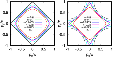
Figure 1: Fermi surface for different filling factors $n$ for the NN model (left panel) and the HTC model (right panel). The value $n=0.7435$ is close to the separatrix value $n=0.743465958$ for the HTC model and $n=1$ is the separatrix value for the NN model.

The energy Fermi surface of one particle is determined by the dispersion relation (3) and depends on the electron filing factor $n$ and related Fermi energy $E_{1}=E_{F}$. Examples of the Fermi surface at various fillings $n$ are shown in Fig. 1. We note that the separatrix case corresponds to the filling $n=0.74346...$ for the HTC model and $n=1$ for the NN model. The separatrix separate bounded and unbounded curves of fixed energy on an infinite plane $(p_{x},p_{y})$ (rotation from libration as for a pendulum). The filling $n$ corresponds to the electron filling while the hole filling is $n_{h}=1-n$. The dependencies of one-particle density $\rho(E_{1})$ of states on energy $E_{1}$ and filling factor $n$ are given in Fig. S1 of SupMat. The density is strongly peaked at $n=1$ (NN model) and $n=0.74346...$ (HTC model) corresponding to the separatrix (and related Van Hove singularity). Indeed, on a separatrix the frequency of motion $\omega_{s}$ becomes zero and thus $\rho(E_{1})\propto 1/\omega_{s}$ becomes singular.

The quantum Hamiltonian of the model with two interacting particles (TIP) has the form:

$$H=H_{1p}^{(1)}\otimes{\bf 1}^{(2)}+{\bf 1}^{(1)}\otimes H_{1p}^{(2)}+\sum_{{\bf r}_{1},{\bf r}_{2}}\bar{U}({\bf r}_{2}-{\bf r}_{1})|{\bf r}_{1},{\bf r}_{2}\rangle\langle{\bf r}_{1},{\bf r}_{2}|$$ (4)

where $H_{1p}^{(j)}$ is the one-particle Hamiltonian (1) of particle $j=1,2$ with positional coordinate ${\bf r}_{j}=(x_{j},y_{j})$ and ${\bf 1}^{(j)}$ is the unit operator of particle $j$. The last term in (4) represents, for the moment, a generic interaction to be specified below.

In absence of interaction ($\bar{U}({\bf r}_{2}-{\bf r}_{1})=0$) the energy eigenvalues of the two electron Hamiltonian (4) with given momenta ${\bf p}_{1}$ and ${\bf p}_{2}$ are:

$$E_{c}({\bf p}_{1},{\bf p}_{2}) =E_{1p}({\bf p}_{1})+E_{1p}({\bf p}_{2})$$ (5)

$$=-4\sum_{{\bf a}\in{\cal A}}t_{\bf a}\cos({\bf p}_{+}\cdot{\bf a}/2)\cos(\Delta{\bf p}\cdot{\bf a})$$

where ${\bf p}_{+}={\bf p}_{1}+{\bf p}_{2}$ is the total momentum (or ${\bf p}_{+}/2=({\bf p}_{1}+{\bf p}_{2})/2$ is the center of mass momentum) and $\Delta{\bf p}=({\bf p}_{2}-{\bf p}_{1})/2$ is the momentum associated to the relative coordinate $\Delta{\bf r}={\bf r}_{2}-{\bf r}_{1}$. Note that the possible values of the components $\Delta p_{\alpha}$ ($\alpha=x,y$) are either integer or half-integer multiples of $2\pi/N$ depending on the center of mass momentum component $p_{+,\alpha}/2$ being an integer or half-integer multiple of $2\pi/N$. For the NN model Eq. (5) becomes $E_{c}({\bf p}_{1},{\bf p}_{2})=-4\sum_{\alpha=x,y}\cos(p_{+\alpha}/2)\cos(\Delta p_{\alpha})$.

Due to the translational invariance of the interaction, it couples only pair momentum states $|{\bf p}_{1},{\bf p}_{2}\rangle$ and $|{\bf p}^{\prime}_{1},{\bf p}^{\prime}_{2}\rangle$ with identical conserved total momentum ${\bf p}_{+}={\bf p}^{\prime}_{+}$, i. e.:

$$\langle{\bf p}^{\prime}_{1},{\bf p}^{\prime}_{2}|\bar{U}|{\bf p}_{1},{\bf p}_{2}\rangle =\delta_{{\bf p}^{\prime}_{+},{\bf p}_{+}}\,U_{p}(\Delta{\bf p}^{\prime}-\Delta{\bf p})\ ,$$ (6)

$$U_{p}(\Delta{\bf p}^{\prime}-\Delta{\bf p}) =\frac{1}{N_{2}}\sum_{\Delta{\bf r}}e^{-i(\Delta{\bf p}^{\prime}-\Delta{\bf p})\cdot\Delta{\bf r}}\bar{U}(\Delta{\bf r})$$ (7)

with $N_{2}=N^{2}$ being the size of the square $N\times N$ lattice and $U_{p}(\Delta{\bf p}^{\prime}-\Delta{\bf p})$ being (proportional to) the discrete Fourier transform of $\hat{U}({\bf r})$. Therefore, the two-particle Hamiltonian (4) can be diagonalized separately for each sector corresponding to a particular value of total momentum ${\bf p}_{+}$.

In htcepjb , the quantum time evolution inside such sectors was computed (for the repulsive Coulomb interaction; see below) using sector eigenstates in $\Delta{\bf r}$-representation with periodic (or anti-periodic) boundary conditions for the case of integer (half-integer) values of $Np_{+,\alpha}/(4\pi)$ ($\alpha=x,y$). In this work, we compute the eigenstates in $\Delta{\bf p}$-representation, using the diagonal energies (5) (minus two times the Fermi energy; see below) in absence of interaction plus the interaction coupling matrix elements (6). We have verified that the resulting eigenstates coincide (in absence of a frozen Fermi sea; see below) up to numerical precision with those of htcepjb once the proper transformation between $\Delta{\bf p}$- and $\Delta{\bf r}$-representations are applied (the half-integer case corresponds now to periodic boundary conditions in $\Delta{\bf p}$-representation but the possible values of $\Delta p_{x,y}$ are half-integer multiples of $2\pi/N$). Furthermore, as explained in htcepjb , we consider symmetric wavefunctions with respect to particle exchange, i.e. with respect to the parity symmetry in the relative momentum $\Delta{\bf p}\to-\Delta{\bf p}$. This case corresponds to an antisymmetric spin-singlet state.

Concerning the choice of the interaction, we consider three cases here :

(i) As in htcepjb , we use a (regularized) repulsive Coulomb type long-range interaction (see Section 7) $\bar{U}({\bf r}_{2}-{\bf r}_{1})=U/[1+r({\bf r}_{2}-{\bf r}_{1})]$ with amplitude $U>0$ and the effective distance $r({\bf r}_{2}-{\bf r}_{1})=\sqrt{\Delta\bar{x}^{2}+\Delta\bar{y}^{2}}$ between the two electrons on the lattice with periodic boundary conditions. (Here $\Delta\bar{x}=\min(\Delta x,N-\Delta x)$; $\Delta\bar{y}=\min(\Delta y,N-\Delta y)$; $\Delta x=x_{2}-x_{1}$; $\Delta y=y_{2}-y_{1}$ and the latter differences are taken modulo $N$, i.e. $\Delta x=N+x_{2}-x_{1}$ if $x_{2}-x_{1}<0$ and similarly for $\Delta y$). For the purpose of numerical diagonalization in $\Delta{\bf p}$-representation, we compute the discrete Fourier transform of this interaction numerically by (7) and we do not use any analytical approximation in this context. We mention that the numerical Fourier transform gives the approximate behavior $U_{p}({\bf k})\sim 1/|{\bf k}|^{3/2}$ for large $|{\bf k}|$ (with ${\bf k}=\Delta{\bf p}^{\prime}-\Delta{\bf p}$) while the analytic 2D-Fourier transform of the (non-regularized) Coulomb interaction (in infinite continuous space) behaves as $U_{p}({\bf k})\sim 1/|{\bf k}|$.

(ii) We also consider the case of an attractive Hubbard interaction $\bar{U}({\bf r}_{2}-{\bf r}_{1})=U\delta_{{\bf r}_{1},{\bf r}_{2}}$ ($U<0$) with $U_{p}(\Delta{\bf p}^{\prime}-\Delta{\bf p})=U/N_{2}=-|U|/N_{2}$ being constant as it was the case for the Cooper problem cooper .

(iii) We also analyze the case of an attractive interaction with d-wave symmetry and interaction coupling matrix elements being $U_{p}(\Delta{\bf p}^{\prime},\Delta{\bf p})=(U/N_{2})g_{\Delta{\bf p}^{\prime}}\,g_{\Delta{\bf p}}$ ($U<0$) with $g_{\Delta{\bf p}}=(\cos\Delta p_{x}-\cos\Delta p_{y})/2$. This interaction cannot simply be obtained from some interaction potential $\bar{U}({\bf r})$ since the matrix elements do not depend on the difference $\Delta{\bf p}^{\prime}-\Delta{\bf p}$. It corresponds to an effective interaction in the context of the Bardeen-Cooper-Schrieffer (BCS) formalism assuming that the superconducting gap obeys the d-wave symmetry $\Delta_{{\bf k}}\sim g_{{\bf k}}$ (see for example Section 4.2 of bansil ). In particular, using this kind of interaction (in the sector ${\bf p}_{+}=0$, i.e. ${\bf p}_{2}=-{\bf p}_{1}=\Delta{\bf p}$), it is easy to verify that the classical BCS variational ansatz indeed produces the gap dependence $\Delta_{{\bf k}}=g_{{\bf k}}\bar{\Delta}$ where the universal parameter $\bar{\Delta}$ is determined by some implicit equation. As with the classical BCS approach, one can argue that this interaction represents certain relevant contributions of the global interaction which is more complicated. We do not claim here that this “d-wave” interaction is “really” present as such in typical HTC-superconductors and our aim is more to compare its influence on pair eigenstates and ground state energies with the attractive Hubbard interaction where no d-wave symmetry is “injected” in the interaction itself.

In the following, we consider a model of two interacting electrons (or holes) with momenta ${\bf p}_{1}={\bf p}_{+}/2-\Delta{\bf p}$, ${\bf p}_{2}={\bf p}_{+}/2+\Delta{\bf p}$ which are excitations of a frozen Fermi sea where momentum states below the Fermi energy $E_{F}$, corresponding to a certain filling value $n$, are occupied. In this case, only values of $\Delta{\bf p}$ are accessible such that both $E_{1p}({\bf p}_{+}/2\pm\Delta{\bf p})>E_{F}$ (or $<E_{F}$ for the hole case). As we will see later, depending on the value of ${\bf p}_{+}$, the structure of available states in the $\Delta{\bf p}$-plane is potentially quite complicated and very interesting. The choice of ${\bf p}_{+}$ itself is actually quite arbitrary, as long as the set of accessible $\Delta{\bf p}$ values is not empty. We may choose ${\bf p}_{+}=0$ for static pairs or ${\bf p}_{+}\neq 0$ for mobile pairs. Occasionally, we will use the notion of a “virtual filling” $n_{v}$ if the center of mass ${\bf p}_{+}/2$ of a pair lies on the Fermi surface at filling $n_{v}$ which may be different from the actually filling $n$ which is used to determine the frozen Fermi sea.

The effective Hamiltonian (for accessible values of $\Delta{\bf p}$), for each sector ${\bf p}_{+}$, also called sector Hamiltonian, has diagonal matrix elements given by $\pm[E_{c}({\bf p}_{1},{\bf p}_{2})-2E_{F}]$ (with “$+$” for electrons and “$-$” for holes) which are coupled by the interaction matrix elements $U_{p}(\Delta{\bf p}^{\prime},\Delta{\bf p})$ according to the different types of interactions we consider. Depending on the interaction, we either use full numerical diagonalization of the effective Hamiltonian (for the case of the Coulomb interaction; see Section 7) or we compute by an efficient method, described in Appendix A.1, the ground state and its energy (for the cases of attractive Hubbard or d-wave interaction; see Sections 3-6) based on the ideas of Cooper cooper and exploiting the rank-1 structure of the interaction matrix elements. As a consequence the energy eigenvalues can be obtained from the numerical solution of an implicit equation of the form of a sum over all two-particle momentum states with each particle being above the frozen Fermi sea (Cooper considered the case of an infinite system where the sum is reduced to an integral cooper ) and the corresponding eigenstates are obtained from an explicit formula once the energy eigenvalues are known (see Appendix A.1 for details). This method allows to significantly reduce the numerical effort and to find the ground state of a Cooper pair for lattices with more than a million sites.

In the remainder of this work, when we speak of eigenstate energies etc. we refer to the eigenvalues of the sector Hamiltonian introduced above, i.e. taking into account a shift with “$-2E_{F}$” and an additional minus sign for the hole case concerning the diagonal matrix elements of this Hamiltonian. Therefore, the ground state energy $E_{\rm min}$ of such a sector Hamiltonian is typically close to zero (corresponding to the Fermi energy) except for the cases where we have a strong gap $\Delta=-E_{\rm min}/2$ with possible negative values of $E_{\rm min}$ and other eigenvalues are positive.

3 Properties of static Cooper pairs

We first consider static Cooper pairs of electrons created by the Hubbard attraction when the total pair momentum is ${\bf p}_{+}=0$. The dependence of the quantity $E_{c}-2E_{F}$ with $E_{c}$ given by (5) on the relative momentum in the $\Delta{\bf p}$-plane is shown in Fig. 2 (left column) for two filling factors $n=0.3;0.74$. The region of the frozen Fermi sea is also shown by white color in Fig. 2 (right column). (In the following, we will refer to this type of figures as “energy landscape” figures.) Thus in the quantum case all transitions induced by interaction between TIP states take place only outside the white zone corresponding to the Cooper approach cooper .

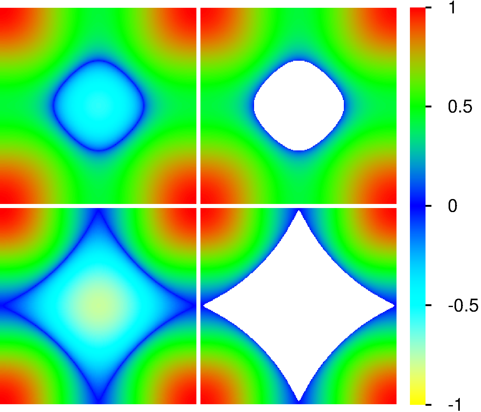
Figure 2: Landscape of kinetic pair energy of particles in the $\Delta{\bf p}$-plane. Left panels show color plots of $E_{c}({\bf p}_{+}/2-\Delta{\bf p},{\bf p}_{+}/2+\Delta{\bf p})-2E_{F}$ for the HTC model in the $\Delta p_{x}$-$\Delta p_{y}$ plane for $-\pi\leq\Delta p_{x,y}<\pi$ in the sector ${\bf p}_{+}=0$. The Fermi energy $E_{F}$ corresponds to the filling factor $n=0.3$ ($n=0.74$) for top (bottom) panels. The colors red (green) correspond to positive maximum (intermediate), blue to zero value and yellow (cyan) to strongest (intermediate) negative values (the shown color bar applies to this and all subsequent color density plot figures of the same style, eventually with nonlinear rescaling to increase the visibility of small value regions). Right panels are as left panels but the forbidden zones of $\Delta{\bf p}$ such that each one-particle energy is below the Fermi energy $E_{F}$, i.e. $E_{1p}({\bf p}_{+}/2-\Delta{\bf p})<E_{F}$ and $E_{1p}({\bf p}_{+}/2+\Delta{\bf p})<E_{F}$, are replaced by white color. For ${\bf p}_{+}=0$ the white zones simply correspond to the colors yellow (cyan) for negative values in the left panel. However, for different sectors with ${\bf p}_{+}\neq 0$ shown in later figures this simple correspondence is no longer true and the structure of white zones is more complicated.

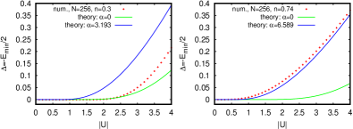
Figure 3: Left (right) panel shows the ground state energy gap $\Delta=-E_{\rm min}/2$ versus absolute Hubbard interaction strength $|U|$ (case of attractive interaction with $U<0$) for ${\bf p}_{+}=0$, for $N=256$, $n=0.3$ ($n=0.74$). (Here $E_{\rm min}$ is the Hubbard ground state energy of the sector Hamiltonian at ${\bf p}_{+}=0$.) The red data points have been obtained by a numerical solution of the implicit eigenvalue equation and coincide up to numerical precision with a full numerical diagonalization. Examples of ground states at specific $U$ values are shown in Fig. S2 of SupMat. The full curves correspond to the analytical approximation assuming a two-particle sector-density of states of the form $\rho_{2}(\varepsilon)=\rho_{2}(0)/[1+\alpha(\varepsilon/\varepsilon_{\rm max})]$ where $\varepsilon_{\rm max}$ is the energy bandwidth in the sector and the parameter $\alpha$ is either zero (green curve; case of constant DOS case) or obtained by a numerical fit (blue curve) from the integrated density of states (see Fig. S4 of SupMat).

We compute numerically, by the method of Appendix A.1, the ground state and its energy for the attractive Hubbard interaction at different values of the interaction strength. The numerically obtained dependence of the gap $\Delta=-E_{\rm min}/2$ on the Hubbard attraction $U$ between electrons (excitation energy above the frozen Fermi sea of electrons) is shown in Fig. 3 for fillings $n=0.3$ and $n=0.74$ where $E_{\rm min}$ is the ground state energy of the effective sector Hamiltonian at ${\bf p}_{+}=0$ (with diagonal matrix elements being $E_{c}({\bf p}_{1},{\bf p}_{2})-2E_{F}$, ${\bf p}_{2,1}={\bf p}_{+}/2\pm\Delta{\bf p}$ as explained above and interaction coupling matrix elements $U_{p}(\Delta{\bf p}^{\prime},\Delta{\bf p})$ for $\Delta{\bf p},\Delta{\bf p}^{\prime}$ outside the forbidden zone due to the frozen Fermi sea). As for the Cooper case cooper the gap sharply drops for small interactions $|U|<1$ and grows strongly for large $|U|>1$.

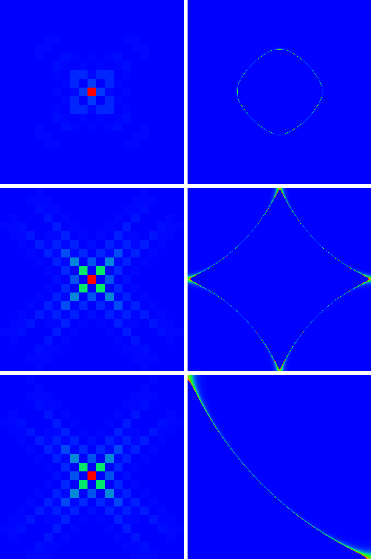
Figure S2: Ground state density plots for the Hubbard interaction, system size $N=256$ (top and center panels) and $N=1024$ (bottom panels), sector ${\bf p}_{+}=0$, and filling factor $n=0.3$, $U=-2.5$ (top) and $n=0.74$, $U=-1$ (center, bottom). Left panels show the ground state in $\Delta{\bf r}$-representation in a zoomed region with $-10\leq\Delta x,\Delta y\leq 10$ (color values outside the zoomed regions are blue) and right panels show the state in $\Delta{\bf p}$-representation (with $-\pi\leq\Delta p_{x,y}<\pi$ for $N=256$ or zoomed top-right square $0\leq\Delta p_{x,y}<\pi$ for $N=1024$). The two particle ground state energies $E_{\rm min}$ (of the sector Hamiltonian) in units of the basic hopping matrix element are $-0.02656$ ($-0.01940$, $-0.01948$) for $n=0.3$, $N=256$, ($n=0.74$, $N=256$ or $n=0.74$, $N=1024$). The state for $N=1024$ in bottom panels is also used for the $g_{k}$-distribution shown in left panels of Fig. 4 (for $U=-1$).

Examples of related ground states at specific $U$ values are shown in Fig. S2 of SupMat for $U=-2.5$ ($n=0.3$) and $U=-1$ ($n=0.74$). In the coordinate space the ground state represents a compact pair state with a size $|\Delta{\bf r}|\sim 2$ and in the momentum space ($\Delta{\bf p}$-plane) the probability of the ground state is concentrated near the Fermi surface shown in Fig. 2. (We also show similar ground states for the case of d-wave interaction at same fillings in Fig. S3 of SupMat).

Fig. 3 also shows the analytical result (18) of Appendix A.1 (blue curve) based on the fit ansatz (17) for the density of states (of diagonal energies of the sector Hamiltonian) assuming a power law decay with exponent $-1$ for large energies. The green curve corresponds to the analytical expression (16) assuming a constant density of states and which is essentially Cooper’s well known result cooper (with different notations/parameters). Further details and analytical expressions of $E_{\rm min}$ for small and strong interactions values are given in Appendix A.1.

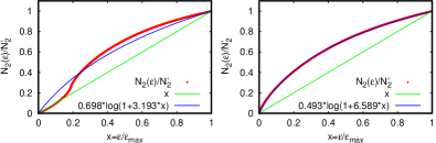
Figure S4: Left (right) panel shows the rescaled integrated two-particle sector-density of states $N_{2}(\varepsilon)/N_{2}^{\prime}$ (red data points) for the sector ${\bf p}_{+}=0$, for $N=256$, $n=0.3$ ($n=0.74$) versus $\varepsilon/\varepsilon_{\rm max}$. Here $N_{2}^{\prime}$ represents the number of accessible levels in the given sector. The green line shows the linear behavior assuming a constant density of states and the blue line shows the fit $N_{2}(\varepsilon)/N_{2}^{\prime}=\log[1+\alpha(\varepsilon/\varepsilon_{\rm max})]/\log(1+\alpha)$ with $\alpha=3.193\pm 0.077$ ($\alpha=6.589\pm 0.017$). These fits are used in Fig. 3.

For the Cooper case cooper the gap $\Delta$ was determined by the attraction strength and the density of states near the Fermi surface since only a small interval corresponding to the Debye energy contributes to the pair formation. In our case all energies above the Fermi sea contribute to the formation of pairs. Thus the approximation of a constant density of states does not work well, especially for $n=0.74$ which is close to the separatrix and the van Hove singularity. For this case the fit ansatz (17) works very well as can be seen in Fig. S4 of SupMat (showing the integrated density of states) and indeed the blue curve in (the right panel of) Fig. 3 coincides very well with the numerical data points for the gap energy.

For $n=0.3$, the situation is different and here the green curve in (the left panel of) Fig. 3 is for modest interaction values ($|U|\lesssim 2.5$) very close to the numerical data points while the blue curve is significantly higher. The reason is that in this case, the density of states is initially, for smaller energies (lower 20%), quite constant (integrated density of states close to a linear function; see red data points and green curve in the left panel of Fig. S4 of SupMat) thus that Cooper’s original expression works very well. However, for larger interaction values in the region $|U|\approx 8$ (not shown in Fig. 3) the blue curve is actually closer to the numerical data points and the reason is that here all energies, also outside the initial region of linear integrated density of states, contribute. Fig. S4 of SupMat shows indeed that also for $n=0.3$ the fit ansatz is more accurate for larger energies (above 20%).

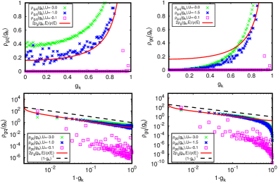
Figure 4: Comparison of the quantum distribution $\rho_{gq}(g_{k})$ (see text), obtained for three interaction values $U$ (green, blue and pink data points), with the renormalized classical density $2\rho_{g}(g_{k})/\rho(E)$ (red line) for the HTC model. Left (right) panels correspond to the attractive Hubbard (d-wave) interaction for $N=1024$, sector with ${\bf p}_{+}=0$ (for the quantum densities) and filling factor $n=0.74$ (for both quantum and classical densities). The relative factor $2/\rho(E)$ applied to the classical density ensures the proper normalization with respect to integration in the range $0\leq g_{k}\leq 1$ since $\int_{-1}^{1}\rho_{g}(g_{k},E)\,dg_{k}=\rho(E)$ where $\rho(E)=0.712$ is the classical density of states at $n=0.74$ (factor $2$ due to $\pm g_{k}$ symmetry). Top panels show a normal representation with a limited maximal value for the $y$-axis and lower panels show a double logarithmic representation using $1-g_{k}$ for the $x$-axis and the full range of density values. The black dashed line in lower panels shows the power law $(1-g_{k})^{-1}$ for comparison (see also Appendix A.2 and Fig. S5 of SupMat).

From Fig. 1 it follows that the angle resolved local density $\rho_{\varphi}(\varphi,E)$ on the energy Fermi surface should significantly depend on the phase angle $\varphi$ of the vector $\Delta{\bf p}=(k_{x},k_{y})\propto(\cos\varphi,\sin\varphi)$. This angle resolved density is proportional to the area between two Fermi curves in Fig. 1 taken at two close filling factors $n$ and $n+\delta n$ and between two close angles $\varphi$ and $\varphi+\delta\varphi$. (See Appendix A.2 for the precise definition, computation and limiting behavior close to the separatrix of $\rho_{\varphi}(\varphi,E)$.)

For $n=0.3$ the Fermi curve is close to a circle and the density $\rho_{\varphi}(\varphi,E)$ is rather constant. However, for $n=0.74$ the Fermi surface is drastically different from a circle and we expect that $\rho_{\varphi}(\varphi,E)$ is minimal for the symmetric case $k_{x}=k_{y}$ or $\varphi\approx\pi/4$ (known as node in ARPES experiments with HTC superconductors kivelson ; proust ; vishik1 ; vishik2 ) and it is maximal for the asymmetric case $k_{x}\approx 0$ or $k_{y}\approx 0$, i.e. $\varphi\approx\pi/2$ or $\varphi\approx 0$ (known as antinode in ARPES).

In the ARPES experiment vishik1 ; vishik2 the d-wave form is typically presented via the parameter $g_{k}=(\cos k_{x}-\cos k_{y})/2$, which can also be used to characterize a certain point on a given Fermi surface instead of $\varphi$, in particular we have $g_{k}\approx 1$ ($0$, $-1$) for $\varphi\approx\pi/2$ ($\pi/4$, $0$) for Fermi curves close to the separatrix curve. Therefore, we prefer to use the $g_{k}$-local density of states on the Fermi surface given by $\rho_{g}(g_{k},E)=\rho_{\varphi}(\varphi,E)/(dg_{k}/d\varphi)$. (See Appendix A.2 for the details of the precise definition, computation and an analytical approximation of $\rho_{g}(g_{k},E)$ for $E$ being close to the separatrix.)

Fig. S5 of SupMat shows this density for the NN- and HTC-model and at different fillings. For the separatrix case, we have a power law $\rho_{g}(g_{k},E)\approx C_{1}/(1-|g_{k}|)$ with a constant $C_{1}$ that can be computed analytically (as a function of the band-structure parameters) and with values $C_{1}\approx 0.025$ ($C_{1}\approx 0.052$) for the NN- (HTC-) model. For Fermi curves close but different from the separatrix curve the density is close to this power law but there is a cutoff at some maximal value $g_{\rm max}<1$ (with a square root singularity close to the cutoff; see Appendix A.2 for more details). The value of $g_{\rm max}$ corresponds to the case where either $k_{x}=0$ and $|k_{y}|$ maximal but typically smaller than $\pi$ (except for the separatrix case) or $k_{y}=0$ and $|k_{x}|$ maximal.

We have also computed the quantum probability density $\rho_{gq}(g_{k})$ for certain ground states (states similar as in Figs. S2, S3 of SupMat) for the cases of the Hubbard and d-wave interaction, at certain interaction strengths, filling $n=0.74$, $N=1024$ and ${\bf p}_{+}=0$. This quantum distribution can be obtained from the interacting ground state $\psi(k)$, with $k=\Delta{\bf p}$ being the momentum in the relative coordinate, from a $g_{k}$-histogram by summing all probabilities $|\psi(k)|^{2}$ for those $k$-values such that $g_{k}$ falls in the same histogram bin with bin-width $\Delta g_{k}=0.01$. To ensure proper normalization with respect to integration in the range $0\leq g_{k}\leq 1$ an additional factor $1/\Delta g_{k}$ has been applied to the histogram values to obtain a properly integration normalized distribution $\rho_{gq}(g_{k})$. Note that this quantity represents a pure $g_{k}$-distribution, a priori for all possible energies, while the classical local density $\rho_{g}(g_{k},E)$ is specific to a certain classical energy $E$. Both quantities are shown and compared for the two cases of the attractive Hubbard and d-wave interaction in Fig. 4 (with a properly corrected normalization of $\rho_{g}(g_{k},E)$ as explained in the figure caption of Fig. 4).

For small $|U|=0.1$ the quantum density is strongly inhomogeneous, essentially with one single peak at $g_{k}=0.995$ with about $99.5$% of probability (only visible in the lower panels with logarithmic representation). The reason is that in this case the ground state is a small perturbation from the pure momentum state with $k$ closest to the Fermi surface. The fact that for this $k$ value we have $g_{k}\approx 1$ is a coincidence (but still with a strongly enhanced probability due to the nearly singular classical density at $g_{k}\approx 1$). For other parameters (fillings $n$, etc.) other $k$- and $g_{k}$-values for these peaks are in principle possible (a similar situation was discussed for eigenstates of rough billiards roughbil ).

For moderate $U=-1;-1.5$ the quantum distribution $\rho_{gq}(g_{k})$ is close to the (renormalized) classical distribution $2\rho_{g}(g_{k},E)/\rho(E)$ in the case of Hubbard interaction but for the d-wave interaction there are still significant differences. To explain this, we remind the expression (11) of Appendix A.1, showing that the eigenstate amplitudes are given by the analytical formula : $\psi(k)\sim a_{k}/(2\Delta+\varepsilon_{k})$ where $\varepsilon_{k}$ represents a diagonal energy matrix element of the effective sector Hamiltonian. The factor $a_{k}$ is either $a_{k}=1$ for the Hubbard interaction or $a_{k}=g_{k}$ for the d-wave interaction.

At very small interactions (e.g. $|U|=0.1$) in the perturbative regime, we also have according to (13) a very small gap $\Delta\sim|U|/N_{2}$ such that only one single $k$-value satisfies the condition $\varepsilon_{k}<2\Delta$ providing an isolated peak of the ground state in $\Delta{\bf p}$-representation. At modest interaction $U=-1$, the gap is significantly larger but still small in comparison to classical energy scales. Therefore, the eigenstate (for the Hubbard case with $a_{k}=1$) is concentrated at $k$- (or $\Delta{\bf p}$-) values close to the Fermi surface with an effective energy width $\approx 2\Delta$ which is perfectly confirmed by Fig. S2 of SupMat. However, the width of this region around the Fermi surface in $k$-space is not uniform, it is enhanced for $k$ values with $|g_{k}|\approx 1$ and reduced for $|g_{k}|\approx 0$. Actually, a closer study of Fig. S2 of SupMat shows that in the region $|g_{k}|\approx 0$ (i.e. $k_{x}\approx k_{y}$) there is still a peak-structure which is due to the finite grid for $N=256$ or $N=1024$.

The reason of this is simply that the distance between the two Fermi curves at $E_{F}$ and $E_{F}+2\Delta$ is quite large at the region close to the separatrix point (with maximal $|g_{k}|$) and quite small at $k_{x}\approx k_{y}$ (with $|g_{k}|\approx 0$) in accordance with the nearly singular behavior of the classical density $\rho_{g}(g_{k},E)$ for $|g_{k}|\approx 1$. When computing the quantum distribution $\rho_{gq}(g_{k})$, we consider a priori all $k$-values but the analytical expression of the amplitudes $\psi(k)\sim 1/(2\Delta+\varepsilon_{k})$ selects automatically the energies closest to the Fermi surface. This explains that (for the Hubbard) interaction the blue data points for $U=-1$ coincide quite well with the red curve for the classical (properly renormalized) density in the left panels of Fig. 4. However, the blue data points still show some fluctuations (at $g_{k}<0.8$) which are due to the finite grid structure of the possible $\varepsilon_{k}$ values.

For the stronger interaction $U=-3$ the green data points deviate significantly from the classical curve, also for the Hubbard case. The reason is that here the gap is significantly larger than for $U=-1$ (see Fig. 3) and the quantum distribution corresponds actually to an energy average of the classical distribution over a quite large energy width of size $2\Delta$ which changes the shape of the distribution (reduction of the singular part at $|g_{k}|\approx 1$, increase of the density at modest values $|g_{k}|<0.9$).

Concerning the d-wave interaction (right panels of Fig. 4), we have the additional factor $g_{k}$ applied to the eigenstate amplitude $\psi(k)$ which provides an additional reduction of the density at $|g_{k}|\approx 0$ (and additional enhancement of the density at $|g_{k}|\approx 1$) which is clearly visible both in Fig. S3 of SupMat and the right panels of Fig. 4.

In conclusion, Fig. 4 and also Figs. S2, S3 of SupMat show, that there are two “d-wave” effects: (i) enhancement of the $g_{k}$-density and wave function amplitudes at $|g_{k}|\approx 1$ simply due the HTC band structure, providing an increased number/area of momentum or $k$ values between two close Fermi curves if $|g_{k}|\approx 1$, (ii) an additional enhancement if the d-wave factor $g_{k}$ is artificially injected in the interaction (case of d-wave interaction).

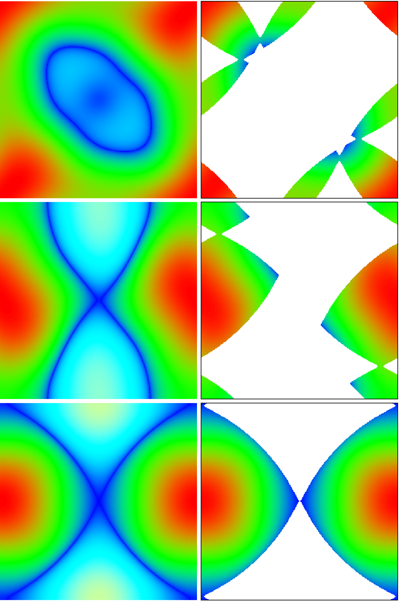
Figure 5: Energy landscape for mobile Cooper pairs. Left panels show color plots of $E_{c}({\bf p}_{+}/2-\Delta{\bf p},{\bf p}_{+}/2+\Delta{\bf p})-2E_{F}$ for the HTC model in the $\Delta p_{x}$-$\Delta p_{y}$ plane for $-\pi\leq\Delta p_{x,y}<\pi$. The Fermi energy $E_{F}$ corresponds to the filling factor $n=0.74$ (in all panels). Top (center, bottom) panel corresponds to the sector ${\bf p}_{+}=2\pi(103,103)/256$ of node case (${\bf p}_{+}=2\pi(46,172)/256$ intermediate case, ${\bf p}_{+}=2\pi(0,248)/256$ antinode case). The three values of ${\bf p}_{+}$ are chosen such that the center of mass momentum ${\bf p}_{+}/2$ is very close to the Fermi surface of virtual filling factor $n_{v}=0.74$ with three cases of $p_{+x}=p_{+y}$, $p_{+x}\approx p_{+y}/4$ and $p_{+x}$ ($p_{+y}$) minimal (maximal). The choice of discrete values is motivated by subsequent quantum computations at $N=256$ with these exact identical parameters. The colors red (green) correspond to positive maximum (intermediate), blue to zero value and yellow (cyan) to strongest (intermediate) negative values (color bar as in Fig. 2). Right panels are as the left panels but the forbidden zones of $\Delta{\bf p}$ (for particle excitations) such that each one-particle energy is below the Fermi energy, i.e. $E_{1p}({\bf p}_{+}/2-\Delta{\bf p})<E_{F}$ and $E_{1p}({\bf p}_{+}/2+\Delta{\bf p})<E_{F}$, are replaced by white color. Note that here the white zones include not only the negative value zones (yellow/cyan) in left panels but also additional zones of positive values due to ${\bf p}_{+}\neq 0$ and the more complicated selection rule using individual one particle energies.

The issue of quantum ergodicity on the Fermi surface, eventually with a peak structure due to a finite grid at modest values of $N$ in the region $k_{x}\approx k_{y}$, is actually quite similar to the problem of rough billiards in the regime of quantum chaos roughbil . Even for the cases where the quantum density $\rho_{gq}(g_{k})$ differs from the classical density $\rho_{g}(g_{k},E)$, the general tendency from classical ergodicity remains valid: $\rho_{gq}(g_{k})$ is small for small $g_{k}$ values (near node) and large for large values of $g_{k}$ (antinode). It is interesting to note that the global dependence of $\rho_{gq}(g_{k})$ at moderate interactions is similar to the experimentally found gap dependence $\Delta(g_{k})$, see for example Fig. 3 in vishik1 for LSCO where $\Delta$ is small for small $g_{k}$ and larger for $g_{k}>0.5$. It is important to stress that a somewhat similar dependence of $\rho_{gq}(g_{k})$ is already visible for the Hubbard interaction which corresponds actually to an s-wave interaction. Thus on this basis, we argue that the d-wave features of HTC superconductors can appear already for s-wave interactions due to the absence of s-wave symmetry for the Fermi surface and the particular band structure of HTC superconductors (point (i) above). We think that this is an important message of this work.

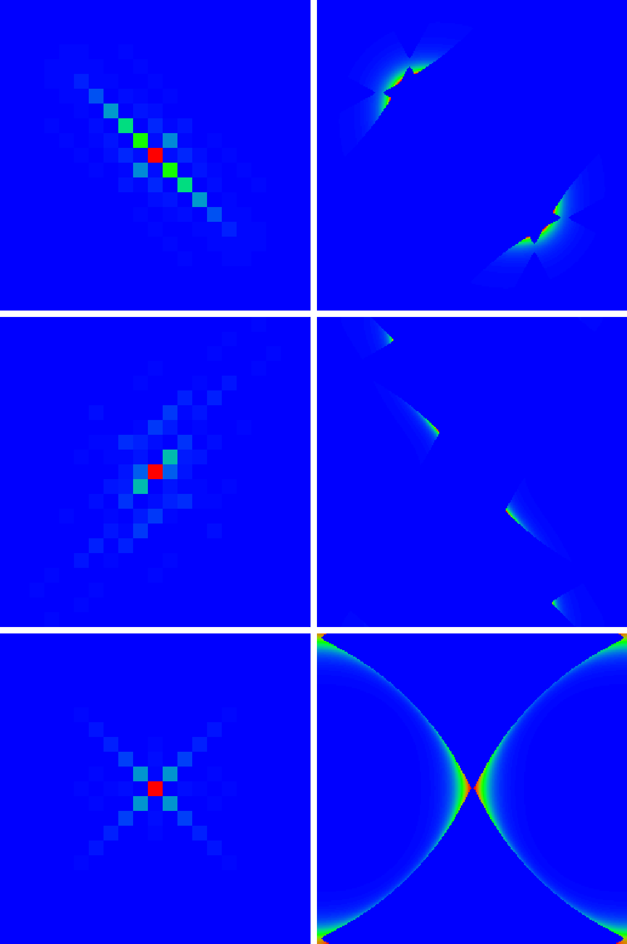
Figure 6: Ground state density plots for the Hubbard interaction, system size $N=256$, particle excitations, filling factor $n=0.74$ and three sectors ${\bf p}_{+}\neq 0$ (same values as in Fig. 5). Top (center, bottom) panels correspond to $U=-4.5$, ${\bf p}_{+}=2\pi(103,103)/256$ ($U=-7$, ${\bf p}_{+}=2\pi(46,172)/256$; $U=-3$, ${\bf p}_{+}=2\pi(0,248)/256$). Left panels show the ground state in $\Delta{\bf r}$-representation in a zoomed region with $-10\leq\Delta x,\Delta y\leq 10$ (color values outside the zoomed regions are blue) and right panels show the state in $\Delta{\bf p}$-representation (with $-\pi\leq\Delta p_{x,y}<\pi$). The two particle ground state energies $E_{\rm min}$ in units of the basic hopping matrix element $t$ are $-0.1360$ ($-0.1427$, $-0.3823$) for top (center, bottom) panels.

4 Properties of mobile Cooper pairs

In the previous Section, we discussed the ground state properties for static Cooper pairs of electrons with zero total momentum ${\bf p}_{+}=0$. However, it is interesting to consider also the case of mobile pairs with ${\bf p}_{+}\neq 0$. Indeed, such mobile pairs can be related to the formation of stripes observed in HTC superconductors (see e.g. stripe1 ; stripe2 and Refs. therein). For particles with a quadratic dependence of kinetic energy on momentum, considered by Cooper cooper , the kinetic energy of a pair is the sum of its internal motion energy and the center of mass motion energy. Thus the kinetic energy of center of mass simply adds a constant and plays therefore no role in the pair formation in a continuous media. The situation is drastically different for LSCO with a rather complex dispersion law for each particle (3). In this case, at ${\bf p}_{+}\neq 0$, the conditions $E_{1p}({\bf p}_{+}/2\pm\Delta{\bf p})>E_{F}$ for allowed transitions above the frozen Fermi sea provide a nontrivial structure for the space of available $\Delta{\bf p}$ values.

Fig. 5 shows examples of the energy landscape of pair energy in the $\Delta{\bf p}$-plane within a fixed ${\bf p}_{+}$ sector without Fermi restrictions (left column) and with restrictions imposed by the frozen Fermi sea (right column) at the filling factor $n=0.74$. The restrictions induced by the frozen Fermi sea create a very complex structure of the accessible $\Delta{\bf p}$-space, with “tongues” and multiple complicated borders, and it depends in a nontrivial manner on the particular choice of ${\bf p}_{+}$. In Fig. 5, we have chosen three examples of ${\bf p}_{+}$ such that the center of mass momentum ${\bf p}_{+}/2$ is very close to the Fermi surface of virtual filling factor $n_{v}=0.74$ with $p_{+x}=p_{+y}$, $p_{+x}\approx p_{+y}/4$ and $p_{+x}$ ($p_{+y}$) minimal (maximal).

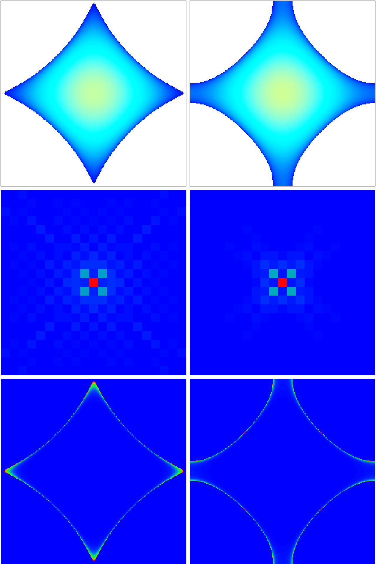
Figure 7: Energy landscape $E_{c}$ and ground states of static hole pairs in the HTC model. Top panels show color plots of $E_{c}({\bf p}_{+}/2-\Delta{\bf p},{\bf p}_{+}/2+\Delta{\bf p})-2E_{F}$ on $\Delta p_{x}$-$\Delta p_{y}$ with $-\pi\leq\Delta p_{x,y}<\pi$ in the sector ${\bf p}_{+}=0$. The forbidden zones for holes of $\Delta{\bf p}$ such that each one-particle energy is above the Fermi energy, i.e. $E_{1p}({\bf p}_{+}/2-\Delta{\bf p})>E_{F}$ and $E_{1p}({\bf p}_{+}/2+\Delta{\bf p})>E_{F}$, are replaced by white color. The Fermi energy $E_{F}$ corresponds to the filling $n=0.74$ (left panels) or $n=0.84$ (right panels). Center and bottom panels show ground state density plots for hole excitations, Hubbard interaction with $U=-1.5$, system size $N=256$ and sector ${\bf p}_{+}=0$. Center panels show the ground state in $\Delta{\bf r}$-representation in a zoomed region with $-10\leq\Delta x,\Delta y\leq 10$ (color values outside the zoomed regions are blue) and bottom panels show the state in $\Delta{\bf p}$-representation (with $-\pi\leq\Delta p_{x,y}<\pi$). The two particle ground state energies $E_{\rm min}$ (of the effective sector Hamiltonian) in units of the basic hopping matrix element are $-0.03734$ ($-0.04222$) for $n=0.74$, ($n=0.84$). The colors red (green) correspond to positive maximum (intermediate), blue to zero value and yellow (cyan) to strongest (intermediate) negative values.

In spite of the complexity of the energy landscape the implicit method for the computation of ground state properties (see Appendix A.1) still works perfectly that allows us to obtain results for lattices with a large number of sites. The ground states for the mobile Cooper pairs with Hubbard attraction are shown in Fig. 6 for parameters of Fig. 5 and interactions values between $U=-3$ and $U=-7$. We see that the ground states correspond to compact pairs in $\Delta{\bf r}$-representation (left column) and their densities in $\Delta{\bf p}$-representation (right column) are concentrated at certain borders of the frozen Fermi sea (“blue” Fermi sea borders with small excitations energies; see right column of Fig. 5). However, to find such nice pairs, it is necessary to considerably increase the value of $|U|$ as compared to static Cooper pairs (at ${\bf p}_{+}=0$). For smaller values of $|U|$ (not shown in Fig. 6), the ground states are perturbative with isolated points in $\Delta{\bf p}$-representation and quite extended in $\Delta{\bf r}$-representation. The reason for the required larger values of $|U|$ is that the sector density of states close to the Fermi surface (number of available states at the blue Fermi sea border regions) is quite reduced as compared to the static case.

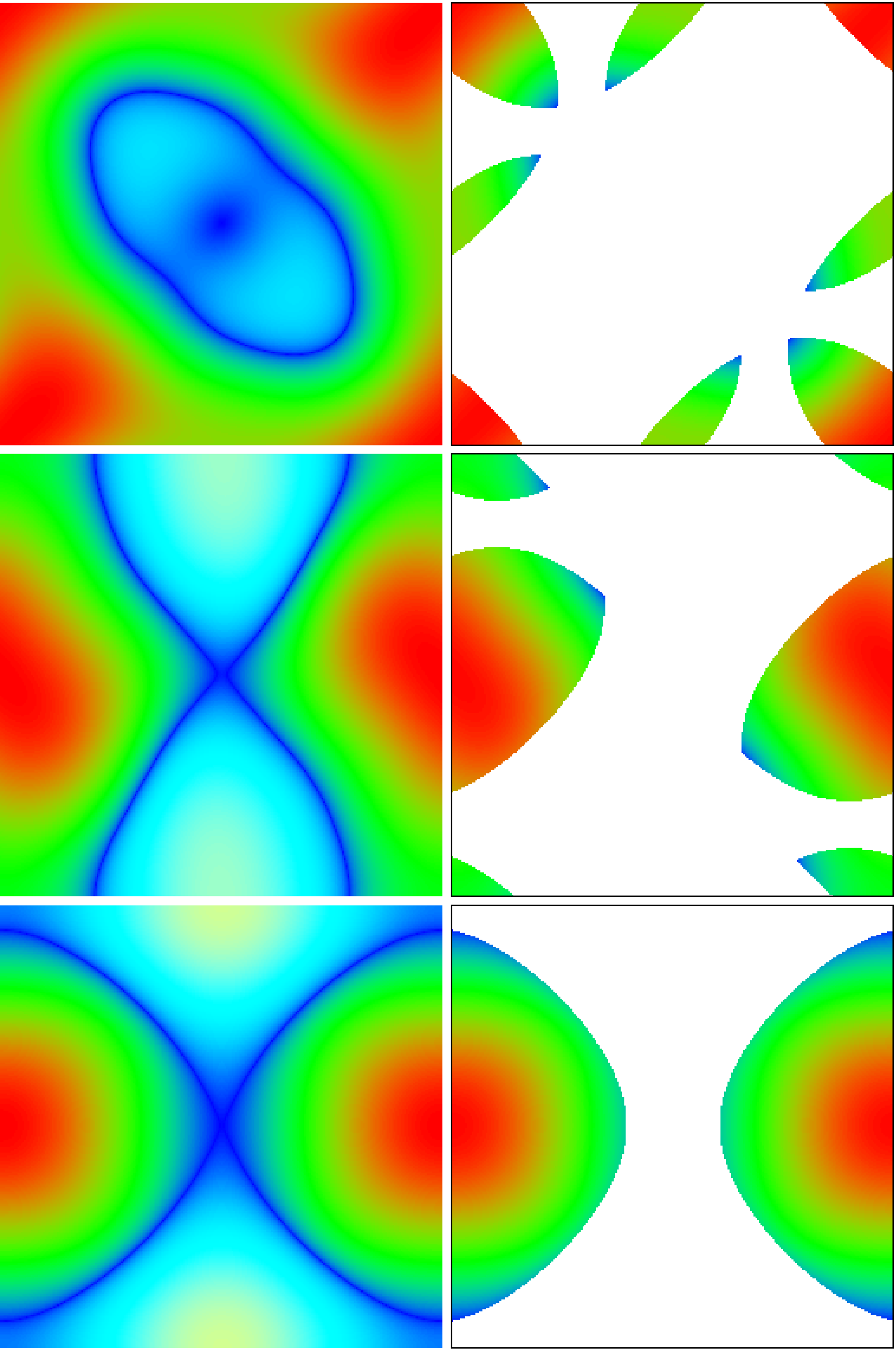
Figure S6: Same as Fig. 5 with particle excitations but for the filling factor $n=0.84$ and the sectors ${\bf p}_{+}=2\pi(106,106)/256$ (top panels), ${\bf p}_{+}=2\pi(52,174)/256$ (center panels) and ${\bf p}_{+}=2\pi(27,256)/256$ (bottom panels) such that the center of mass momentum ${\bf p}_{+}/2$ is very close to the Fermi surface of virtual filling factor $n_{v}=0.84$ with three cases of $p_{+x}=p_{+y}$, $p_{+x}\approx p_{+y}/4$ and $p_{+x}$ ($p_{+y}$) minimal (maximal).

Results similar to those of Figs. 5, 6 are presented for another filling factor $n=0.84$ (and virtual filling $n_{v}=0.84$ for the choice of ${\bf p}_{+}/2$) in Figs. S6, S7 of SupMat.

We discuss more features of mobile Cooper pair in the next Sections.

5 Gap dependence on hole doping in LSCO for static pairs

Up to now, we discussed the properties of Cooper pairs of electrons at fixed electron doping $n$. However, for LSCO the superconducting phase is formed by doping of holes. This feature can be easily incorporated in the framework of the Cooper approach considering hole excitation of the frozen Fermi sea at fixed hole doping $n_{h}=1-n$. Mathematically, one applies two fermionic hole creation operators (being two electron annihilation operators) to the frozen Fermi sea and as usual in the context of particle-hole transformation the one-body matrix elements between such hole-pair states acquire an additional negative sign while two-body matrix elements due to interactions are not changed.

In particular, now the set of accessible $\Delta{\bf p}$ values must satisfy the condition of both electrons, associated to holes, being below the Fermi energy (i.e. being in the Fermi sea) with : $E_{1p}({\bf p}_{+}/2\pm\Delta{\bf p})<E_{F}$ and the diagonal matrix elements in the effective sector Hamiltonian are $-[E_{c}({\bf p}_{1},{\bf p}_{2})-2E_{F}]>0$ (with ${\bf p}_{2,1}={\bf p}_{+}/2\pm\Delta{\bf p}$ and $E_{c}$ given by (5)) since it costs energy to excite holes and the interaction coupling matrix elements $U_{p}(\Delta{\bf p}^{\prime},\Delta{\bf p})$ are unchanged. For convenience, we do not apply the sign change in the following energy landscape figures for holes (figures of style of Figs. 2, 5) such that the forbidden white zones for holes correspond to positive values of $E_{c}({\bf p}_{1},{\bf p}_{2})-2E_{F}>0$ (for the simple case ${\bf p}_{+}=0$).

In this Section, we first consider the case of static hole pairs with ${\bf p}_{+}=0$. Examples of the energy landscape with the frozen Fermi sea for hole dopings $n_{h}=1-n$ at $n=0.74,0.84$ are shown in top panels of Fig. 7. The ground states for these $n_{h}$ values (and $U=-1.5$) with attractive Hubbard interaction of holes are also shown in this figure. The results show that the pairs are very compact in the coordinate space and in the momentum space they are located at the (inside) vicinity of the Fermi surface with an effective width in momentum space being larger (smaller) if $\Delta p_{x}\approx\pm\pi$, $\Delta p_{y}\approx 0$ or $\Delta p_{x}\approx 0$, $\Delta p_{y}\approx\pm\pi$ ($\Delta p_{x}\approx\Delta p_{y}$ respectively) in a similar way for electron pair states visible Fig. S2 of SupMat (located at the outside vicinity of the Fermi surface). The same approach also works for the case of attractive d-wave interaction giving similar results for the ground state energies and eigenstates but with an additional suppression of momentum wave function amplitudes in regions $\Delta p_{x}\approx\Delta p_{y}$ (not shown in figures here but similar to Fig. S3 of SupMat).

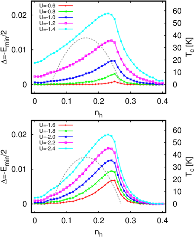
Figure 8: Gap dependence on hole doping $n_{h}$ in the HTC model of LSCO. Shown is the gap energy $\Delta=-E_{\rm min}/2$ for hole excitations as a function of doping value $n_{h}=1-n$ for $N=1024$ and the sector ${\bf p}_{+}=0$. The left vertical scale gives the energy values in units of the basic hopping matrix element $t$ and the right vertical scale gives the corresponding value of the critical temperature $T_{c}$ obtained from $\Delta=1.764\,k_{B}\,T_{c}$ and using $t=0.43\,$eV. Top (bottom) panel corresponds to the Hubbard (d-wave) interaction with $U=-0.6,-0.8,-1,-1.2,-1.4$ ($U=-1.6,-1.8,-2,-2.2,-2.4$) for bottom to top curves. The parabolic grey dashed curve corresponds to the formula $T_{c}=T_{c0}[1-(\frac{n_{0}-n_{h}}{n_{1}})^{2}]$ with $T_{c0}=38\,K$, $n_{0}=0.16$, $n_{1}=0.11$ obtained from experimental data markiewicz .

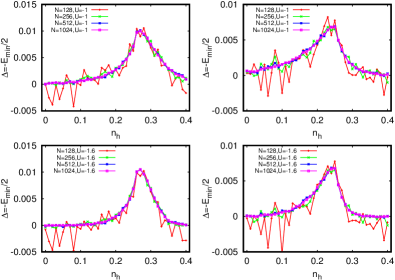
Figure S8: Convergence of gap energy $\Delta=-E_{\rm min}/2$ with increasing values of $N=128,\,256,\,512,\,1024$ and for the sector ${\bf p}_{+}=0$ as a function of doping value $n_{h}=1-n$. The energy values are given in units of the basic hopping matrix element $t$. Top (bottom) panels correspond to the Hubbard (d-wave) interaction with $U=-1$ ($U=-1.6$). Left (right) panels correspond to electron (hole) excitations.

We also computed the gap dependence on hole doping in LSCO for the attractive Hubbard and d-wave interactions at different interaction values $U$ and lattice size $N=1024$ (more than a million lattice sites). The results are shown in Fig. 8 and the convergence of gap values with increasing lattice size from $N=128$ to $N=1024$ is shown in Fig. S8 of SupMat for an intermediate interaction value for both interaction cases. The curves exhibit still strong fluctuations at $N=128$ but the two curves at $N=512$ and $N=1024$ are nearly identical showing that $N=1024$ is sufficient to have gap values in the limit of infinite lattice size.

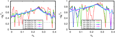
Figure 9: Ground state quantum average $\langle g_{k}^{2}\rangle$ for hole pairs as a function of doping $n_{h}=1-n$ for $N=1024$ and the sector ${\bf p}_{+}=0$, with $g_{k}=(\cos(k_{x})-\cos(k_{y}))/2$ and ${\bf k}=\Delta{\bf p}=(k_{x},k_{y})$ being the quantum momentum space of the ground state at given doping $n_{h}$ (${\bf p}_{+}={\bf k}_{+}$ at $\hbar=1$) . Left (right) panel corresponds to the Hubbard (d-wave) interaction with $U=-0.6,-0.8,-1,-1.2,-1.4$ ($U=-0.6,-1,-1.4,-1.8,-2.2$) for red, green, blue, pink, cyan curves respectively. The grey dashed line at the value $\langle g_{k}^{2}\rangle=0.25$ corresponds to the uniform average over all values ${\bf k}=(k_{x},k_{y})$ with probability homogeneously distributed in the plane $-\pi<k_{x,y}<\pi$.

The gap values allow to obtain the critical temperature $T_{c}$ of superconductivity using the standard relation $\Delta=1.764k_{B}T_{c}$ (here $k_{B}$ is the Boltzmann constant and temperature $T_{c}$ is measured in Kelvin) tinkham . In Fig. 8, we also present the dependence of $T_{c}$ on hole doping $n_{h}$ in LSCO. For the Hubbard case at $U=-1.2$ we obtain the maximal $T_{c}\approx 36K$ (at the hopping $t=0.43\,$eV markiewicz ) being rather similar to the maximal $T_{c0}=38\,K$ obtained experimentally (see Fig.11 in markiewicz and experimental Refs. therein). The LSCO experimental results are satisfactorily described by the doping dependence $T_{c}=T_{c0}[1-(\frac{n_{0}-n_{h}}{n_{1}})^{2}]$ with the optimal doping $n_{0}=0.16$ and $n_{1}=0.11$ markiewicz . The Hubbard results at $U=-1.2$ (at $t=0.43\,$eV this corresponds to $U=0.516\,$eV) give the closest similarity of the $T_{c}$ dependence on hole doping $n_{h}$. Still the numerical data at $U=-1.2$ give a somewhat different shape of the curve $T_{c}(n_{h})$ as compared to experimental data. Thus, the optimal doping is at $n_{h}=0.24$ for $U=-1.2$ (it slightly changes with $U$). It is slightly below the doping value $n_{hs}=1-n_{s}\approx 0.26$ corresponding to the separatrix (see Fig. 1). Indeed, the density of states is maximal at the van Hove singularity which significantly contributes to the gap increase if the Fermi surface of holes is located slightly below the separatrix value $n_{hs}\approx 0.26$. In this case we have $E_{F}>E_{s}$ ($E_{s}$ being the separatrix energy) and the accessible hole states include the region of $E_{s}$ that contributes to increase of the (sector) density of states. Our numerical data provides a dependence $T_{c}(n_{h})$ on $n_{h}$ which seems to be rather close to the experimental data. We attribute certain differences (shift of the maximum position) to the fact that for LSCO three-dimensional effects significantly affect the hopping parameters and the separatrix position as discussed in fresard . In particular, Fig. 15 of fresard indicates a separatrix position closer to $n=0.84$ ($n_{h}=0.16$) due to 3D and multiple band effects where the $k_{z}$ quantum number also plays a role. Furthermore, our computations are based on the simple Hubbard interaction which may be different from the real effective interaction between holes.

We also show the dependence $T_{c}(n_{h})$ for the attractive d-wave interaction, in the bottom panel of Fig. 8, with curves being rather similar to the Hubbard case. However, a somewhat stronger attractive interaction strength $U=-2$ ($U=-0.86\,$eV for $t=0.43\,$eV) is required to have a maximal $T_{c}$ value close the experimental value $T_{c}=38\,K$ while the shape of the curves $T_{c}(n_{h})$ remains rather similar to the Hubbard case. Thus the comparison of $T_{c}(n_{h})$ curves for Hubbard and d-wave interactions indicates that the shapes of the Fermi surface curves is mainly at the origin of gap dependence on doping in the HTC model.

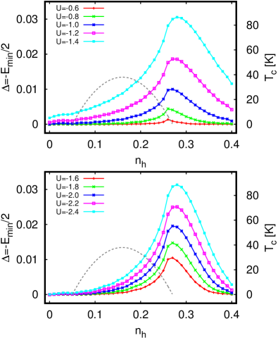
Figure S9: As Fig. 8 but for electron excitations.

In Fig. S9 of SupMat, we also show for completeness the dependence of $T_{c}(n)$ on $n_{h}=1-n$ for Cooper pairs of electrons which have a rather similar structure as the hole case but in both cases there is certain a asymmetry around the maximum which is different between holes and electrons. Thus at doping $n_{h}=0.2$ and $U=-1.2$ the gap for electron pairs is about 50% smaller than for hole pairs.

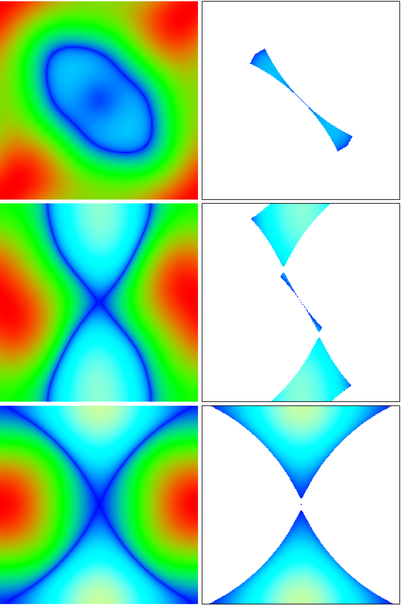
Figure 10: Energy landscape for mobile hole pairs. Left panels show color plots of $E_{c}({\bf p}_{+}/2-\Delta{\bf p},{\bf p}_{+}/2+\Delta{\bf p})-2E_{F}$ for the HTC model in the $\Delta p_{x}$-$\Delta p_{y}$ plane for $-\pi\leq\Delta p_{x,y}<\pi$. The Fermi energy $E_{F}$ corresponds to the filling factor $n=0.74$ (in all panels). Top (center, bottom) panel corresponds to the sector ${\bf p}_{+}=2\pi(103,103)/256$ (${\bf p}_{+}=2\pi(46,172)/256$, ${\bf p}_{+}=2\pi(0,248)/256$). The three values of ${\bf p}_{+}$ are chosen such that the center of mass momentum ${\bf p}_{+}/2$ is very close to the Fermi surface of virtual filling factor $n_{v}=0.74$ with three cases of $p_{+x}=p_{+y}$, $p_{+x}\approx p_{+y}/4$ and $p_{+x}$ ($p_{+y}$) minimal (maximal). The choice of discrete values is motivated by subsequent quantum computations at $N=256$ with these exact identical parameters. The colors red (green) correspond to positive maximum (intermediate), blue to zero value and yellow (cyan) to strongest (intermediate) negative values. Right panels are as the left panels but the forbidden zones of $\Delta{\bf p}$ (for hole excitations) such that each one-particle energy is above the Fermi energy, i.e. $E_{1p}({\bf p}_{+}/2-\Delta{\bf p})>E_{F}$ and $E_{1p}({\bf p}_{+}/2+\Delta{\bf p})>E_{F}$, are replaced by white color. Note that here the white zones include not only the positive value zones (red/green) in left panels but also additional zones of negative values due to ${\bf p}_{+}\neq 0$ and the more complicated selection rule using individual one particle energies.

To characterize the d-wave structure of the ground state we compute the value of the quantum average $\langle g_{k}^{2}\rangle$ over the ground state in momentum representation (with $k$ being $\Delta{\bf p}$ and $g_{k}=(\cos(k_{x})-\cos(k_{y}))/2$). The dependence of $\langle g_{k}^{2}\rangle$ on hole doping $n_{h}$ is shown in Fig. 9 for different values of $U$ for Hubbard and d-wave interactions. At small $|U|$ the interactions and gap are too weak and the discreteness of momentum values at finite lattice size leads to strong fluctuations of $\langle g_{k}^{2}\rangle$ with $n_{h}$. This happens because at small $|U|$ only few specific $k$ values, closest to the Fermi surface, contribute to the ground state (a similar effect is discussed in detail for rough billiards in roughbil ). However, for moderate interactions ($|U|\geq 1$ for Hubbard and $|U|\geq 1.4$ for d-wave cases), corresponding to $T_{c}$ values close to experimental ones (see Fig. 8), the system size $N=1024$ is sufficiently close to the infinite $N$ limit with a smooth dependence of $\langle g_{k}^{2}\rangle$ on $n_{h}$. As for $\Delta(n_{h})$ shown in Fig. 8 the average $\langle g_{k}^{2}\rangle$ has also a maximum close to the optimal doping $n_{h}\approx 0.26$ corresponding to the separatrix (van Hove singularity). However, in contrast to $\Delta(n_{h})$ the maximum is not very smooth and the lowest values of $\langle g_{k}^{2}\rangle$ (in the interval $0\leq n_{h}\leq 0.4$) are quite large, about $\sim 65$ % of the maximal value. The maximal values themselves $\langle g_{k}^{2}\rangle\approx 0.75$ (Hubbard case) and $0.87$ (d-wave case) are rather high and close to unity which corresponds to a strong concentration of the wavefunction in the vicinity of the antinode $k_{x}\approx 0,k_{y}\approx\pm\pi$ (or inverse).

Such a concentration is indeed visible for the ground state in momentum space shown in Fig. 7. We note that for the whole considered range of dopings $0\leq n_{h}\leq 0.4$ the obtained values of $\langle g_{k}^{2}\rangle$ are significantly larger than the value $0.25$ corresponding to a homogeneous distribution of probability over all $k_{x},k_{y}$ values in the interval $[-\pi,\pi]$. Using the classical local density $\rho_{g}(g_{k})\sim 1/(1-|g_{k}|)$ with a cutoff $|g_{k}|\leq g_{\rm max}$, where $g_{\rm max}<1$ is the maximal possible value of $|g_{k}|$ (for Fermi curves close to the separatrix curve; see Appendix A.2), one can expect for the Hubbard case the analytical estimate : $\langle g_{k}^{2}\rangle_{\rm cl.}\approx 1-3/(2|\ln(1-g_{\rm max})|)$ which provides theoretically unity for the exact separatrix curve but with a rather strong logarithmic correction even if $1-g_{\rm max}\ll 1$ which explains the rather larger values in Fig. 9 (significantly above $0.25$) but still somewhat smaller than unity.

For the d-wave interaction, we remind that the momentum wave function amplitudes are essentially multiplied with $g_{k}$ (in comparison to the Hubbard wave function amplitudes at same gap value) and we expect that $\langle g_{k}^{2}\rangle_{q,{\rm d-wave}}\approx\langle g_{k}^{4}\rangle_{\rm cl.}/\langle g_{k}^{2}\rangle_{\rm cl.}\approx 1-7/(12|\ln(1-g_{\rm max})|)$, with a reduced logarithmic correction explaining the somewhat larger values (closer to unity) in the right panel of Fig. 9.

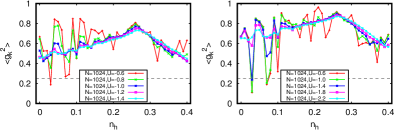
Figure S10: As Fig. 9 but for electron excitations.

We note that similar results are obtained for the dependence of $\langle g_{k}^{2}\rangle$ on $n_{h}$ for electron pairs (see Fig. S10 of SupMat).

The fact, that for both interactions the average $\langle g_{k}^{2}\rangle$, is significantly above the uniform average $0.25$, confirms the findings of Section 3 that the HTC-band structure alone induces a kind of d-wave preference in classical phase space (larger distance between two neighbor Fermi curves if $|g_{k}|\approx 1$) or for quantum states (with more occupied grid points in the regions close to the Fermi surface if $|g_{k}|\approx 1$). Therefore, to observe a d-wave dependence it is not necessary to inject a d-wave dependence in the interaction as such, as can be seen in the results of Fig. 8 and Fig. 9 for the (s-wave) Hubbard interaction. For the d-wave interaction, the “d-wave” effect is somewhat enhanced but this enhancement is not the dominant part. Furthermore, the HTC-band structure also breaks the central symmetry in the vicinity of optimal doping values.

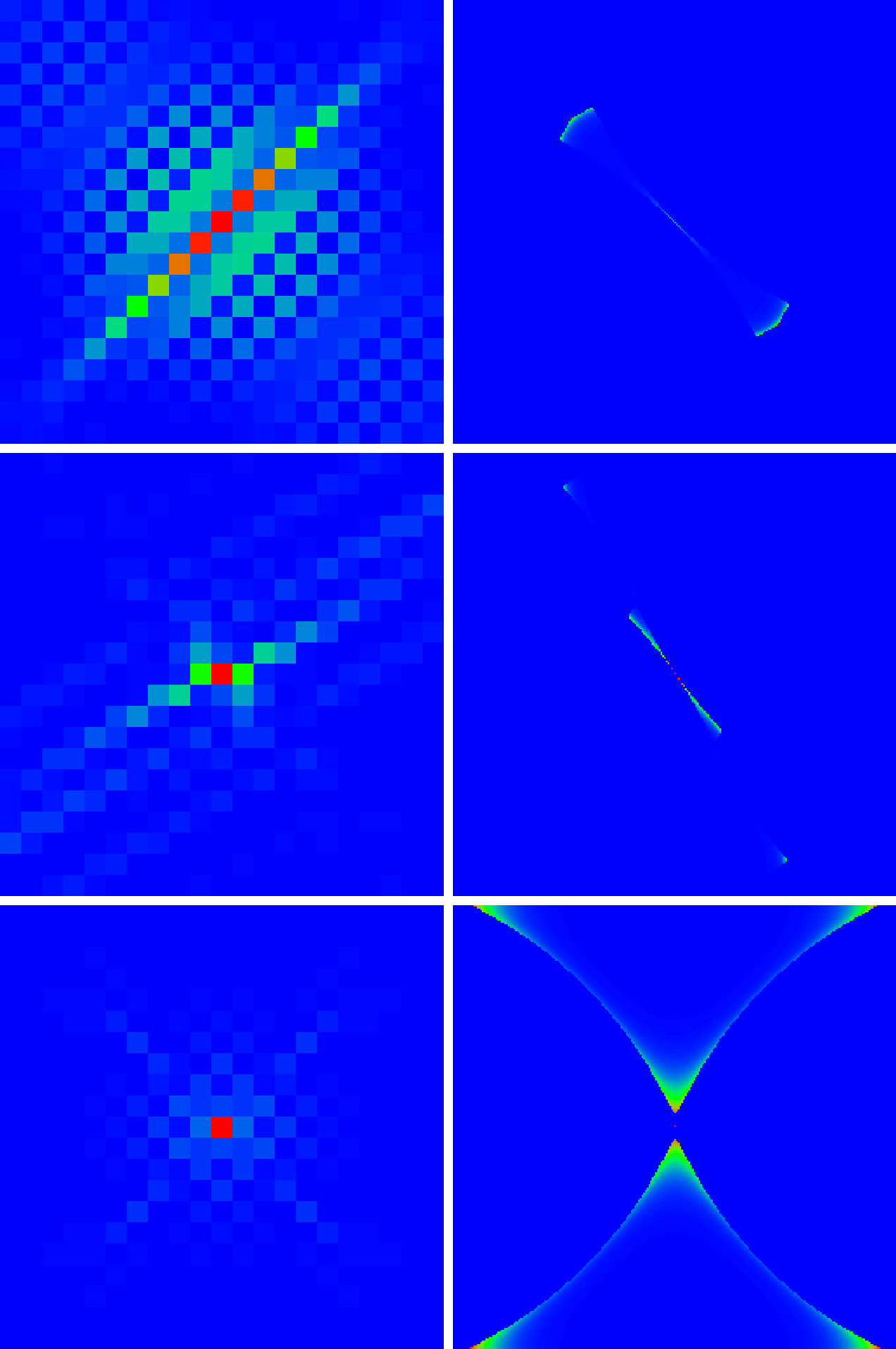
Figure 11: Ground state density plots for the Hubbard interaction, system size $N=256$, hole pairs, filling factor $n=0.74,n_{h}=1-n$ and three sectors ${\bf p}_{+}\neq 0$ (same values as in Fig. 5). Top (center, bottom) panels correspond to $U=-8$, ${\bf p}_{+}=2\pi(103,103)/256$ ($U=-6$, ${\bf p}_{+}=2\pi(46,172)/256$; $U=-4$, ${\bf p}_{+}=2\pi(0,248)/256$). Left panels show the ground state in $\Delta{\bf r}$-representation in a zoomed region with $-10\leq\Delta x,\Delta y\leq 10$ (color values outside the zoomed regions are blue) and right panels show the state in $\Delta{\bf p}$-representation (with $-\pi\leq\Delta p_{x,y}<\pi$). The two hole ground state energies $E_{\rm min}$ (of the sector Hamiltonian and in units of the basic hopping matrix element) are $-0.03424$ ($-0.07144$, $-0.1884$) for top (center, bottom) panels.

6 Gap for mobile Cooper pairs of holes

In this Section, we discuss the case of mobile pairs of holes with ${\bf p}_{+}\neq 0$. Similarly as in Section 4, we use a virtual filling $n_{v}=0.74$ (and $n_{v}=0.84$ for SupMat figures) corresponding to certain center of mass values ${\bf p}_{+}/2$ being (very close) to the Fermi surface with filling $n_{v}$.

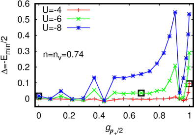
Figure 12: Gap energy $\Delta=-E_{\rm min}/2$ for hole pairs as a function of $g_{{\bf p}_{+}/2}=[\cos(p_{+x}/2)-\cos(p_{+y}/2)]/2$ for $n=0.74,n_{h}=1-n$ and 21 sector values of ${\bf p}_{+}$ such that the values of the center of mass ${\bf p}_{+}/2$ lie uniformly on the line of virtual filling factor $n_{v}=0.74$ between the positions of $p_{+x}=p_{+y}$, with $g_{{\bf p}_{+}/2}=0$, and $p_{+x}\approx 0$, $p_{+y}\approx 2\pi$, with $g_{{\bf p}_{+}/2}\approx 1$. The three curves correspond to the three interaction values used in Fig. 11 and the data points with black squares correspond to the three states shown in Fig. 11 with $g_{{\bf p}_{+}/2}=0$ ($\approx 0.7$, $\approx 1$) for top (center, bottom) row therein. Data are obtained at $N=256$.

An example of the energy landscape for mobile pairs is shown in Fig. 10 for the filling factor $n=0.74,n_{h}=1-n$ and the virtual filling factor being very close to this value $n_{v}=0.74$ (up to discreteness lattice effects). We see that the energy landscape changes significantly depending on the value of ${\bf p}_{+}/2$ on the virtual Fermi surface at $n_{v}$. The landscape is shown for three cases of $p_{+x}=p_{+y}$, $p_{+x}\approx p_{+y}/4$ and $p_{+x}$ ($p_{+y}$) minimal (maximal). Even more striking are the changes of the zones of accessible $\Delta{\bf p}$ values shown in the right column of Fig. 10 due to the condition $E_{1p}({\bf p}_{+}/2\pm\Delta{\bf p})<E_{F}$ (see also discussion at the beginning of Section 5). For $p_{+x}=p_{+y}$ these zones are composed of a quite small island with a dumbbell form. For $p_{+x}\approx p_{+y}/4$ this island is strongly reduced but two extra pieces around $\Delta{\bf p}=(0,\pm\pi)$ have been added. Finally, for $p_{+x}=0$ and $p_{+y}$ maximal the island has (nearly) disappeared and the extra pieces have increased in size with curved boundaries.

Examples of ground states of hole pairs for parameters of Fig. 10 are shown in Fig. 11. Similarly, as in Fig. 6, the ground states correspond to compact pairs in $\Delta{\bf r}$-representation (left column) with a size decreasing with the increase of the gap $\Delta$. Their densities in $\Delta{\bf p}$-representation (right column) are again concentrated at certain borders of the frozen Fermi sea (“blue” Fermi sea borders with energies close to the Fermi surface; see right column of Fig. 10). In particular, the (momentum) ground state for $p_{+x}=p_{+y}$, is concentrated on the outside borders of the dumbbell island.

The important feature of these ground states is that the gap values $\Delta=-E_{\rm min}/2$ are rather modest even if the Hubbard interaction strength is by a factor $4$ or even more higher as compared to the case of static pairs of Fig. 8. Similarly as with mobile electron pairs (see Section 4) it is necessary to consider rather large interaction amplitudes $|U|$ between -4 and -8 to find nice pair states.

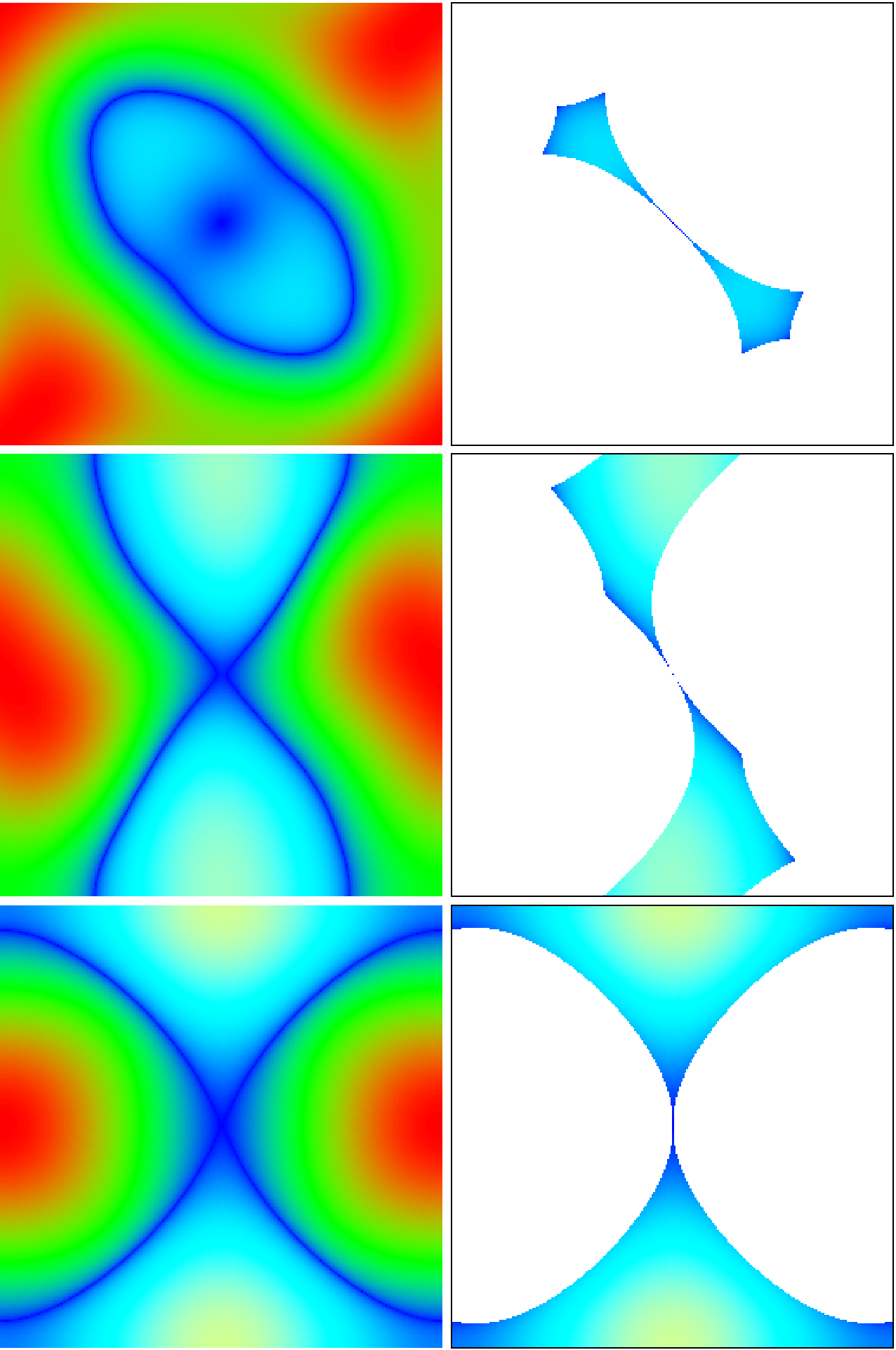
Figure S11: Same as Fig. 10 with hole excitations but for the filling factor $n=0.84$ and the sectors ${\bf p}_{+}=2\pi(106,106)/256$ (top panels), ${\bf p}_{+}=2\pi(52,174)/256$ (center panels) and ${\bf p}_{+}=2\pi(27,256)/256$) (bottom panels) such that the center of mass momentum ${\bf p}_{+}/2$ is very close to the Fermi surface of virtual filling factor $n_{v}=0.84$ with three cases of $p_{+x}=p_{+y}$, $p_{+x}\approx p_{+y}/4$ and $p_{+x}$ ($p_{+y}$) minimal (maximal).

It is convenient to express the gap dependence on $p_{+x}$, $p_{+y}$ via the quantity $g_{{\bf p}_{+}/2}=[\cos(p_{+x}/2)-\cos(p_{+y}/2)]/2$ which characterizes the position of the center of mass ${\bf p}_{+}/2$ on the (virtual) Fermi surface (we note that this quantity is different from $g_{k}$ used in the previous Sections since now $k$ corresponds to the center of mass ${\bf p}_{+}/2$ while previously it was given by the relative momentum $\Delta{\bf p}$). The dependence of the gap $\Delta$ on this quantity is shown in Fig. 12 for three interactions values $U=-4,-6,-8$ and for 21 uniformly distributed data points on the virtual Fermi surface. The main observations from Fig. 12 can be listed as follows: the gap is very small at $g_{{\bf p}_{+}/2}\approx 0$ (symmetry point $p_{+x}=p_{+y}$) and is highest at $g_{{\bf p}_{+}/2}\approx 1$ (asymmetry point $p_{+x}=0$, $p_{+y}$ maximal, or inverse). This can be understood from the fact that the number of accessible states is significantly larger for $g_{{\bf p}_{+}/2}\approx 1$ than for $g_{{\bf p}_{+}/2}\approx 0$ (small dumbbell island) or for other intermediate states (with intermediate $g_{{\bf p}_{+}/2}$) as it is well seen in the right column panels of Figs. 10 and 11. The gap appears at rather large values $|U|$ for the Hubbard interaction as compared to the case of static pairs (with ${\bf p}_{+}=0$; see Section 5). Similar results for another case, $n=n_{v}=0.84$, are shown in Figs. S11, S12, S13 of SupMat.

We also considered the case of small values of $|{\bf p}_{+}|\to 0$ (nearly static pairs) at modest interaction strength $|U|=1$ (case of presence of a modest gap $\Delta\approx 0.06$ for holes and $\Delta\approx 0.1$ for electrons at $n=0.74$ and ${\bf p}_{+}=0$ and zero gap at $n_{v}=0.74$ with non-zero ${\bf p}_{+}$ values of Figs. 10 and 11). It turns that for $N=512$ the gap rapidly disappears with increasing value of $|{\bf p}_{+}|$ at $|{\bf p}_{+}|\gtrsim(2\pi l)/512$ with $l\approx 7-10$ for particles and $l\approx 3-5$ for holes. These borders correspond to very small virtual filling values $n_{v}\sim 10^{-4}-10^{-3}$.

In global, the results of this Section show that it is possible to have coupled mobile pairs with an energy gap but the required (attractive) interaction amplitude should be $4-8$ times larger as compared to the case of static pairs.

7 Pairs with Coulomb repulsion

Figure 13: The pair weight $w_{N/6}$ defined as the quantum probability for $|\Delta x|\leq N/6$ and $|\Delta y|\leq N/6$ is shown as a function of the pair excitation energy $E$ (eigenvalue of the sector Hamiltonian and with $E=0$ corresponding to the Fermi level; see Section 2 for details) for the case of repulsive Coulomb interaction with $U=2$, HTC model and filling factor $n=0.74$. Top (bottom) panel corresponds to hole excitations with ${\bf p}_{+}=2\pi(207,\,207)/512$, sector dimension $N_{2}^{\prime}=3040$ and $N=512$ with center of mass ${\bf p}_{+}/2$ being on the Fermi surface for virtual filling factor $n_{v}=0.74$ (particle excitations with ${\bf p}_{+}=2\pi(113,\,113)/256$, sector dimension $N_{2}^{\prime}=8737$, $N=256$ and $n_{v}=1$). The blue line shows $N_{2}(E)/N_{2}^{\prime}$ with $N_{2}(E)$ being the number of levels below $E$. The energy values with strong energy derivative of this quantity, corresponding to strong peaks of sector density of states, coincide with the main peaks of $w_{N/6}$ for well defined close pair states. The dashed black line indicates the value $w_{N/6}=1/9$ for uniform ergodic states on the whole lattice. The energy landscape for these parameters is shown in Fig. 14. The data points with black squares correspond to the states shown in Figs. 15, 16 (and in related Figs. S14, S15 of SupMat). Additional data, especially raw png figures for pair states with $w_{N/6}>0.4$, for these two cases and also for $N=512$ for the parameters of the bottom panel are available at ourwebpage .

In this Section, we present results of pair eigenstates for the repulsive Coulomb interaction (see case (i) in the discussion of Section 2) combined with a frozen Fermi sea. In previous works prr2020 ; htcepjb , the time evolution of electron pairs in NN and HTC lattices was studied for free pairs (in absence of a frozen Fermi sea) showing that the Coulomb repulsion can lead to Coulomb pair formation due to the appearance of an effective narrow or flat band when the total pair momentum is ${\bf p}_{+}\approx(\pm\pi,\pm\pi)$. Such a mechanism is rather interesting but it is important to understand if such states can have a gap ($E_{\rm min}<0$) or not and if such Coulomb pairs can exist in presence of a frozen Fermi surface and at which energies.

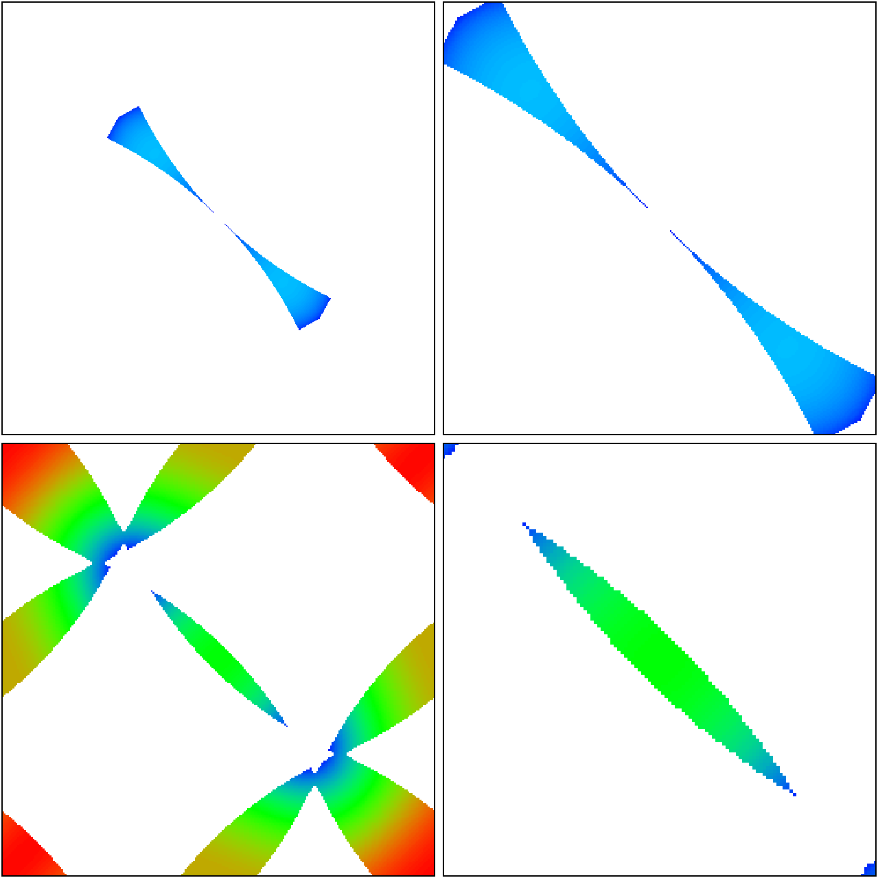
Figure 14: Colored allowed (forbidden white) zones in $\Delta{\bf p}$-plane (see captions of Figs. 5, 10 for details). Top (bottom) panels correspond to the parameters of top (bottom) panel of Fig. 13 with filling factor $n=0.74$, hole (electron) excitations, ${\bf p}_{+}=2\pi(207,\,207)/512$ and $N=512$ (${\bf p}_{+}=2\pi(113,\,113)/256$ and $N=256$). Right (left) panels show the full momentum cell: $-\pi\leq\Delta p_{x,y}<\pi$ (zoomed center square: $-\pi/2\leq\Delta p_{x,y}<\pi/2$) in $\Delta{\bf p}$-plane. Note that top left panel here corresponds nearly exactly to the top right panel of Fig. 10 (with a slight difference in ${\bf p}_{+}$ due to different choices of $N$).

Due to a more complicated structure of coupling matrix elements the effective method of Appendix A.1 is not suitable and we determine the eigenstates and energies of the sector Hamiltonian (see Section 2 for details of its definition) by numerical full diagonalization. For this, we consider two particular cases:

(i) Hole excitations at $n=0.74$ with one single value of ${\bf p}_{+}$ such that $p_{+x}=p_{+y}=2\pi(207/512)$ corresponding to $n_{v}=0.74$ and sector dimension $N_{2}^{\prime}=3040$ at $N=512$. Note that the sector dimension is strongly reduced with respect to $N_{2}=N^{2}=512^{2}$ due to the small fraction of available states (case of dumbbell island visible in top right panel of Fig. 10) allowing to choose the rather large system size $N=512$.

(ii) Electron excitations at $n=0.74$, also with one single value of ${\bf p}_{+}$ such that $p_{+x}=p_{+y}=2\pi(113/256)$ corresponding to $n_{v}=1$ and sector dimension $N_{2}^{\prime}=8737$ at $N=256$. We have also computed the eigenstates and energies for the larger case $N=512$ with $p_{+x}=p_{+y}=2\pi(225/512)$, $N_{2}^{\prime}=35030$, and verified that all physical conclusions remain valid. However, for practical reasons, we present here figures and the discussion only for the case $N=256$ (reduced number of data points and better visible eigenfunction figures at $N=256$, especially in momentum space). The choice of ${\bf p}_{+}$ corresponding to $n_{v}=1\neq n=0.74$ is motivated by its proximity to the “optimal” value $(\pi,\pi)$ found in prr2020 ; htcepjb and the fact that the zone of allowed $\Delta{\bf p}$ values covers the vicinity of $\Delta{\bf p}=0$ which is actually a point of “negative mass” as we will see below (at $n_{v}=0.74$ and $p_{+x}=p_{+y}$ the region $\Delta{\bf p}=0$ would be in the forbidden zone; see top right panel of Fig. 5).

Additional data, especially raw png figures for pair states, for these cases (i), (ii) and (ii) for $N=512$ are available at ourwebpage .

We also studied many other parameters (other choices of $n$, $n_{v}$, ${\bf p}_{+}$ with ${\bf p}_{+}/2$ being on different points of the virtual Fermi surface etc.) and in all cases the ground state energy $E_{\rm min}$ (of the sector Hamiltonian) was found to be positive such that there is no gap (in the framework of this approach) for repulsive Coulomb interaction. However, we discovered different mechanisms of pair formation at different excitation energies (sometimes close to the Fermi energy, sometimes at quite high excitation energies). The two specific examples above provide eigenstates for all interesting cases which we will discuss below.

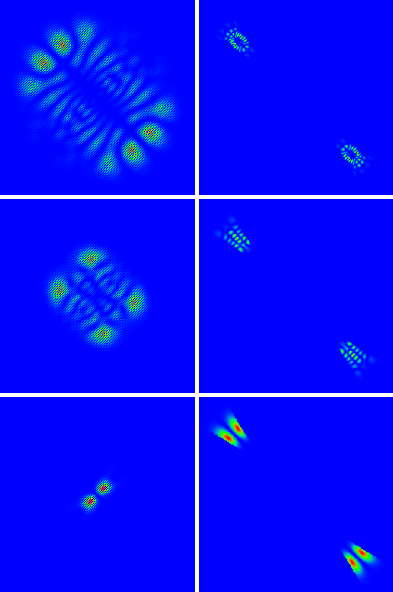
Figure 15: Three strong pair eigenstates for the parameters of top panel of Fig. 13 (holes, $n=n_{v}=0.74$, $N=512$) for energies close to $0.3$ and marked by black squares therein. Left (right) columns correspond to the $\Delta{\bf r}$- ($\Delta{\bf p}$-) representation showing the two times zoomed center square for both cases: $-N/4\leq\Delta x,\Delta y<N/4$ ($-\pi/2\leq\Delta p_{x,y}<\pi/2$). The panels in $\Delta{\bf p}$-representation correspond to the top right panel of Fig. 14 concerning the identification of allowed and forbidden zones. Top (center, bottom) row corresponds to the eigenstates with level number $2974$ ($3011$, $3037$), energy $0.3342$ ($0.3485$, $0.4371$) and pair weight $w_{N/6}=0.8164$ ($0.9900$, $0.9853$). Note that $N_{2}^{\prime}=3040$ is the maximal possible level number for the largest energy (in the corresponding ${\bf p}_{+}$-sector).

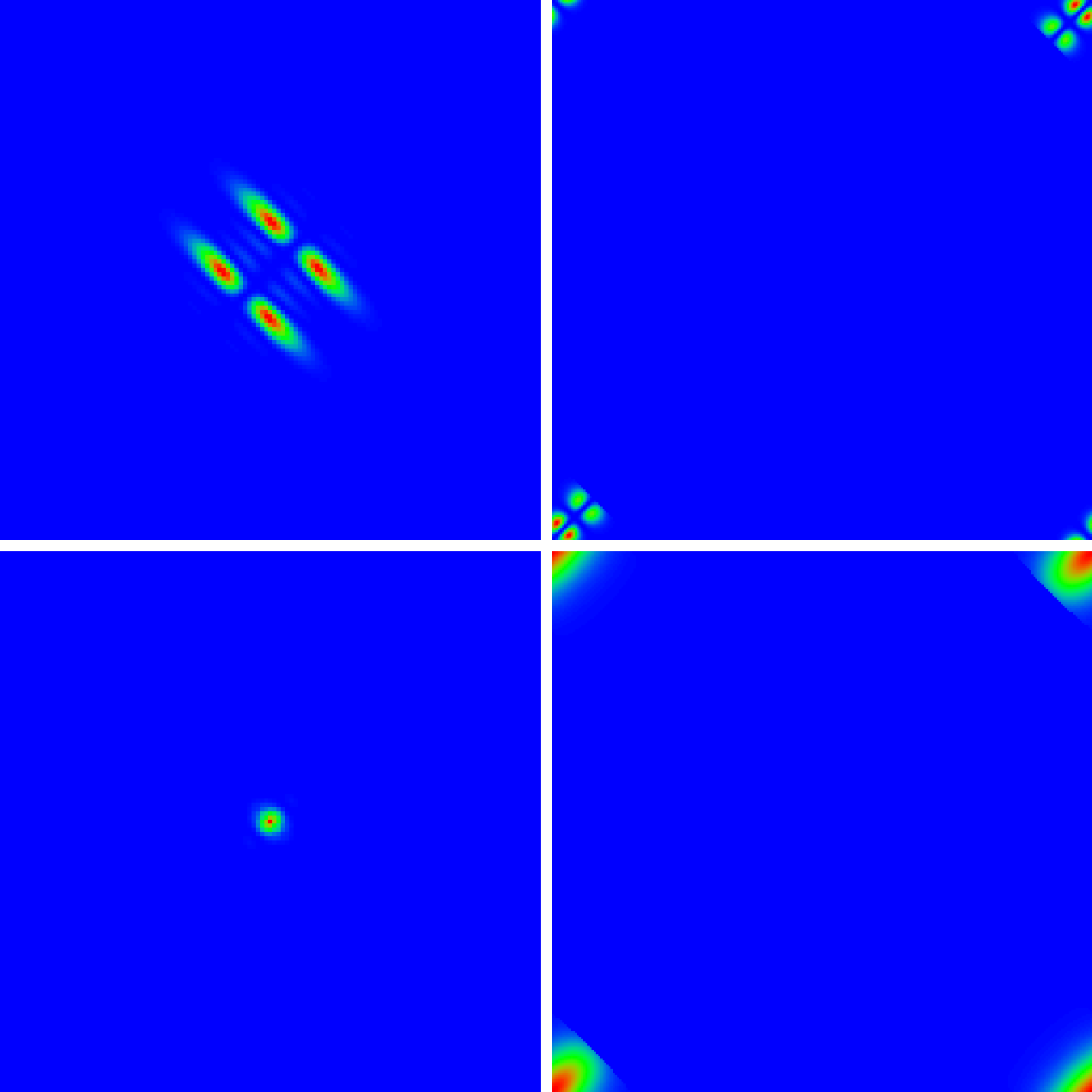
Figure 16: Two strong pair eigenstates for the parameters of bottom panel of Fig. 13 (particles, $n=0.74$, $n_{v}=1$, $N=256$) of the third strong peak of large $w_{N/6}$-values for energies close to $3.5$-$4$ and marked by black squares therein. Left (right) columns correspond to the $\Delta{\bf r}$- ($\Delta{\bf p}$-) representation showing the two times zoomed center square: $-N/4\leq\Delta x,\Delta y<N/4$ (full momentum cell: $-\pi\leq\Delta p_{x,y}<\pi$). The panels in $\Delta{\bf p}$-representation correspond to the bottom left panel of Fig. 14 concerning the identification of allowed and forbidden zones. Top (bottom) row corresponds to the eigenstates with level number $8732$ ($8737$), energy $3.571$ ($4.048$) and pair weight $w_{N/6}=0.9970$ ($0.9976$). Here $N_{2}^{\prime}=8737$ is the maximal possible level number for the largest energy (in the corresponding ${\bf p}_{+}$-sector).

To identify interesting Coulomb pairs at excited energies we compute for each eigenstate the quantity $w_{N/6}(E)$ defined as the quantum probability of $|\Delta x|\leq N/6$ and $|\Delta y|\leq N/6$ (obtained by summing $|\psi(\Delta{\bf r})|^{2}$ over $\Delta{\bf r}$ satisfying this condition with $\psi(\Delta{\bf r})$ being an eigenstate in $\Delta{\bf r}$-representation; see also Eq. (9) and text below of htcepjb for the definition of the similar quantity $w_{10}$). In this work, we replace the width $10$ with $N/6$ since many nice pair states are still quite extended. Values of $w_{N/6}(E)$ significantly above the ergodic value $1/9$ (i.e. close to $1$) indicate pair states (at certain energies) which are quite well localized around $\Delta{\bf r}\approx 0$. We have also computed other quantities such as the quantum averages $\langle|\Delta{\bf r}|\rangle$, $e^{\langle\ln|\Delta{\bf r}|\rangle}$, $\langle\bar{U}(\Delta{\bf r})\rangle$ or the inverse participation ratio in $\Delta{\bf r}$-representation, providing the same typical energies at which nice pair states appear.

Fig. 13 shows $w_{N/6}(E)$ (red data points) as a function of the excitation energy $E$ (eigenvalues of the sector Hamiltonian with diagonal matrix elements $\pm(E_{c}({\bf p}_{1},{\bf p}_{2})-2E_{F}$; see discussion of Section 2 for details) for both above examples (i) in top panel and (ii) in bottom panel. In addition, also the normalized integrated (sector) density of states $N_{2}(E)/N_{2}^{\prime}$, (fraction of states with energies below $E$; blue curves) are shown.

For the case (i), there is one peak of strong pair states, with $w_{N/6}(E)$ close to 1, at the top of the energy spectrum, mostly at $E\approx 0.3$ and with a few states going up $E=0.4-0.7$ (energy measured in units of the basic hopping matrix element $t$). For the case (ii), there are three main peaks at energies $E\approx 0.9,\,2.1-2.2$ and $3-3.5$ (top of the spectrum for the third peak). In addition there also two secondary peaks behind the first two peaks at $E\approx 1.2,\,2.6$. We observe at all main peak positions for both cases an enhanced slope of $N_{2}(E)/N_{2}^{\prime}$ just before the energy corresponding to the peak indicating a strongly enhanced density of states at these energy values. For the case (ii) at $E\approx 0.9$ this effect is bit less strong, but still visible, as compared to the other peaks.

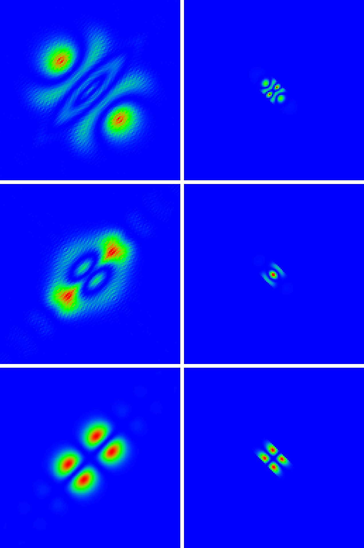
Figure S14: Three strong pair eigenstates for the parameters of bottom panel of Fig. 13 (electrons, $n=0.74$, $n_{v}=1$, $N=256$) of the first peak of large $w_{N/6}$-values for energies close to $0.9$ and marked by black squares therein. Left (right) columns correspond to the $\Delta{\bf r}$- ($\Delta{\bf p}$-) representation showing the two times zoomed center square for both cases: $-N/4\leq\Delta x,\Delta y<N/4$ ($-\pi/2\leq\Delta p_{x,y}<\pi/2$). The panels in $\Delta{\bf p}$-representation correspond to the bottom right panel of Fig. 14 concerning the identification of allowed and forbidden zones. Top (center, bottom) row corresponds to the eigenstates with level number $2573$ ($2638$, $2679$), energy $0.9131$ ($0.9390$, $0.9550$) and pair weight $w_{N/6}=0.9173$ ($0.9069$, $0.9761$). Here $N_{2}^{\prime}=8737$ is the maximal possible level number for the largest energy (in the corresponding ${\bf p}_{+}$-sector).

To understand these observations and the physical nature of the pair states at these energies, we show in Fig. 14 the energy landscape of allowed $\Delta{\bf p}$ values together with the forbidden zones and in Figs. 15, 16 and Figs. S14, S15 of SupMat examples of pair states at the peak energies marked by black squares in Fig. 13. Top panels of Fig. 14 shows again the dumbbell island for the case (i) (see also top right panel of Fig. 10) with a 50% zoom in the right panel and bottom panels correspond to the case (ii) which is somewhat similar to the right panel of Fig. 5 but with an additional cigar-shape island in the region around $\Delta{\bf p}=0$ which appears due to the modified virtual filling $n_{v}=1$ with respect to $n_{v}=0.74$ in Fig. 5 (both with $p_{+x}=p_{+y}$).

The panels of Fig. 14, have to be viewed together with the eigenstate figures in $\Delta{\bf p}$-representation (right panels of Figs. 15, 16 and Figs. S14, S15 of SupMat). For example, for the case (i) we see that the eigenstate densities in $\Delta{\bf p}$-space of the three pairs shown in Fig. 15 are concentrated a the outer border of the dumbbell island. The densities in $\Delta{\bf r}$-space are localized around $\Delta{\bf r}=0$ with a width of about 33% (state of top panels), 25% (state of center panels) and 5% (state of top panels) of the available lattice showing that the width decreases when the energies approaches the top of the spectrum. These pair states are created by a combined mechanism of top spectrum, narrow band and island structure because at the top of the spectrum the repulsive Coulomb interaction behaves like an attractive interaction (at the bottom of the spectrum) confining the particles to a well defined pair.

The eigenstates shown in Fig. 16 correspond to the case (ii) at the top of spectrum (third main peak at $E\approx 3.5-4.5$) with $\Delta{\bf p}$-densities concentrated at the regions $\Delta{\bf p}\approx(\pm\pi,\pm\pi)$ corresponding to red maximum regions in bottom panels of Fig. 14. Here the pair creation mechanism is essentially due to the top spectrum (also negative mass; see below) and there is no strong island effect. Also the effective band is not very narrow (one may argue that the red zone region in bottom panels of Fig. 14 constitutes an effective narrow band). The width in $\Delta{\bf r}$ space (around $\Delta{\bf r}=0$) decreases very strongly when approaching the top of the spectrum.

The states shown in Fig. S14 of SupMat for the first main energy peak ($E\approx 0.9$) of the case (ii) are very interesting. Their $\Delta{\bf p}$-densities are localized around $\Delta{\bf p}=0$ which constitutes a local energy maximum (center green zone of cigar shape island in bottom panels of Fig. 14). This point is actually characterized by two negative eigenvalues of the Hessian matrix obtained by expanding $E_{c}$ given in (5) up to second order in $\Delta{\bf p}$. As can be seen in (bottom right panel) of Fig. S16 of SupMat, the symmetric value of ${\bf p}_{+}/2$ (i.e. with $p_{+x}=p_{+y}$) falls for $n_{v}=1$ clearly in one of the droplet regions where both eigenvalues are negative providing a point of negative mass with a clear local maximum in $\Delta{\bf p}$ space. Therefore, the pairs at $E\approx 0.9$ are created by the mechanism of negative mass which is similar to the mechanism of top spectrum where the repulsive Coulomb interaction confines particles. In $\Delta{\bf r}$-space the densities are again localized around $\Delta{\bf r}$ with width values between 15-25% of the lattice.

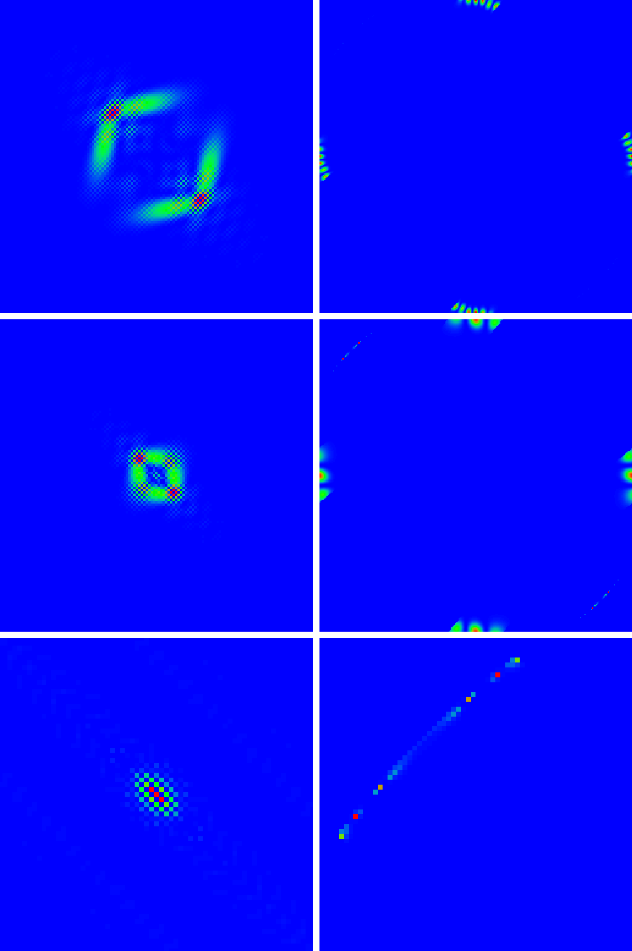
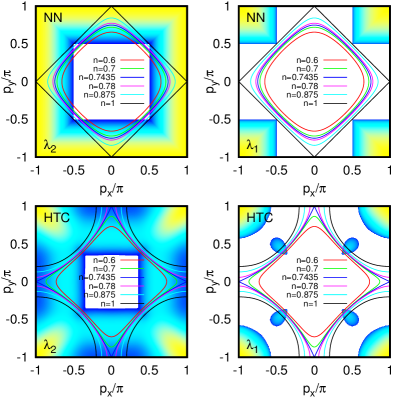
Figure S15: Three strong pair eigenstates for the parameters of bottom panel of Fig.13 (electrons, $n=0.74$, $n_{v}=1$, $N=256$) of the second peak (and the small peak behind it) of large $w_{N/6}$-values for energies close to $2.2$-$2.6$ and marked by black squares therein. Left (right) columns correspond to the $\Delta{\bf r}$- ($\Delta{\bf p}$-) representation. Top and center rows show the two times zoomed center square: $-N/4\leq\Delta x,\Delta y<N/4$ (full momentum cell: $-\pi\leq\Delta p_{x,y}<\pi$). The bottom row shows the four times zoomed center square: $-N/8\leq\Delta x,\Delta y<N/8$ (left panel) or the four times zoomed top left momentum corner: $-\pi\leq\Delta p_{x,y}<-\pi/2$ (right panel) with other non-blue values in the (non-shown) bottom right momentum corner being the mirror image of the top left momentum corner (with $\Delta p_{x,y}\to\pi-\Delta p_{x,y}$). The top and center panels in $\Delta{\bf p}$-representation correspond to the bottom left panel of Fig.14 concerning the identification of allowed and forbidden zones (for bottom $\Delta{\bf p}$-panel the top left corner has to be used). Top (center, bottom) row corresponds to the eigenstates with level number $6606$ ($6718$, $7062$), energy $2.165$ ($2.271$, $2.614$) and pair weight $w_{N/6}=0.9800$ ($0.9658$, $0.2862$). Here $N_{2}^{\prime}=8737$ is the maximal possible level number for the largest energy (in the corresponding ${\bf p}_{+}$-sector).

Example states of the second main energy peak ($E\approx 2.2-2.6$) of the case (ii) are shown in Fig. S15 of SupMat. These states correspond to the regions of olive color (in bottom panels of Fig. 14) either at $\Delta{\bf p}\approx(0,\pm\pi)$, $\Delta{\bf p}\approx(\pm\pi,0)$ (for top and center panels with $E\approx 2.2$) or $\Delta{\bf p}\approx\pm 0.9(-\pi,\pi)$ (bottom panels with $E\approx 2.6$). Here the points $\Delta{\bf p}\approx(0,\pm\pi)$, $\Delta{\bf p}\approx(\pm\pi,0)$ correspond to regions with a local maximum in one direction and finite width in $\Delta{\bf p}$-space in the orthogonal direction due to the forbidden zone thus leading to a quasi-negative mass situation (note that Fig. S16 of SupMat does not apply to this case since $\Delta{\bf p}\neq 0$). The case of bottom panels is special, since there is no local maximum in $\Delta{\bf p}$-space at $\Delta{\bf p}\approx\pm 0.9(-\pi,\pi)$, and despite the optical appearance of a very close pair in $\Delta{\bf r}$-space the actual value of $w_{N/6}(E)\approx 0.3$ (see the black square data point at $E\approx 2.6$ in bottom panel of Fig. 13) is quite small such that about 70% of the quantum probability is still uniformly distributed over the full lattice. However, the other 30% of probability produce a very strong peaked density around $\Delta{\bf r}=0$ with large maximum values such that the uniform background is not visible in the color plot.

In all cases, we see that the region of allowed $\Delta{\bf p}$ values has a quasi 1D-structure in $\Delta{\bf p}$-space (cigar or dumbbell shape island or finite width around the red or olive regions). Since these regions correspond (except for the special case of bottom panels of Fig. S15 of SupMat) to a global or local maximum of $E_{c}$ in $\Delta{\bf p}$-space this explains that, at the energies slightly below the maximum value, the density of states is strongly enhanced (see blue curves in Fig. 13). In $1D$ the free momentum density of states is singular at a spectral border and in quasi-$1D$ with a finite width there should be still a strong enhancement.

We mention that we have also studied a further case similar to (ii) but with $n_{v}=1.25$ (instead of $n_{v}=1$) such that the symmetric value ${\bf p}_{+}=(\pi,\pi)$ is exactly at the optimal point found in htcepjb . In this case, the three main peaks visible in the bottom panel of Fig. 13 merge into one single peak at the (modified) top of the spectrum at $E\approx 2.2-2.7$ and both green/olive zones (for $n=1$) at $\Delta{\bf p}=0$ or $\Delta{\bf p}\approx(0,\pm\pi)$, $\Delta{\bf p}+\approx(\pm\pi,0)$ become red (for $n=1.25$) and all three maxima have now the same value. In particular, the negative mass point at $\Delta{\bf p}=0$ corresponds now to a global maximum being degenerate with the other maxima at $\Delta{\bf p}\approx(0,\pm\pi)$, $\Delta{\bf p}+\approx(\pm\pi,0)$ and $\Delta{\bf p}\approx(\pm\pi,\pm\pi)$ and the $\Delta{\bf p}$-densities of pair states are concentrated at these points.

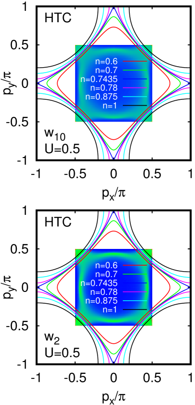
Figure S17: Fermi surface for different filling factors as in Fig. 1 superimposed with color plots for the pair formation probabilities $w_{10}$ and $w_{2}$ of the HTC model computed in Ref.htcepjb for $N=192$ from the long time evolution of an initially localized electron pair in relative coordinate propagating with the repulsive Coulomb interaction $U=0.5$. The color plots in the center of mass momentum ${\bf p}={\bf p}_{+}/2$ are obtained by symmetric extension of the data of Fig. 4 in Ref.htcepjb . Note that the data of htcepjb correspond to a free electron pair moving in an empty system without any other electrons (absence of frozen Fermi sea). The regions of strong pair formation probability close to ${\bf p}\approx(\pm\pi/2,\pm\pi/2)$ correspond also to regions of double negative mass eigenvalues shown in Fig. S16. (Note that at ${\bf p}=(\pm\pi/2,\pm\pi/2)$ there are exact red data points for maximum values in the color plot. However, due the global figure scale these data points are not well visible.) As in Fig. S16, the filling values correspond to the virtual filling $n_{v}=n$.

These observations provide an additional explanation of the results of htcepjb with optimal pair formation (in absence of a frozen Fermi sea) at ${\bf p}_{+}=(\pm\pi,\pm\pi)$. In Fig. S17, we show again the data of Fig. 4 of htcepjb in a color plot superimposed with the Fermi surface for certain fillings $n=n_{v}$ by identifying ${\bf p}={\bf p}_{+}/2$. The value of ${\bf p}_{+}/2\approx 0.4-0.45(\pi,\pi)$ (i.e. $n_{v}=0.74$ or $n_{v}=1$) of the above two cases (i) and (ii) correspond to green zones of an enhanced pair formation probability. The optimal point ${\bf p}_{+}/2=0.5(\pi,\pi)$ corresponds to a red data point data (however, not very well visible in the figure).

Thus the three main mechanisms of pair formation by Coulomb repulsion are: narrow or flat band local spectrum structure as discussed in prr2020 ; htcepjb ; negative effective mass for the pair energy so that a repulsion works as an effective attraction; restricted area (e.g. cigar shape or dumbbell islands) of states accessible for interaction induced transitions above the frozen Fermi sea. At the same time a quasi-1D structure of allowed $\Delta{\bf p}$ zones leads also to an enhanced density of states for a small energy intervall slightly below typical pair energies (peak positions of $w_{N/6}$). We also point out that, in the framework of this approach, Coulomb repulsion does not lead to a gap with a ground state energy below the Fermi surface.

8 Discussion

In this work, we apply the Cooper approach cooper to study the formation of coupled pairs of two interacting particles, holes or electrons, in a tight-binding model of La-based cuprate superconductors. The one-particle band structure of such systems is obtained from advanced numerical analysis markiewicz ; bansil ; fresard based on modern methods of quantum chemistry. We consider three types of interactions being: attractive Hubbard and d-wave type interactions and the standard repulsive Coulomb interaction. Following the Cooper approach cooper , the interaction induced transitions are taking place only over the pair states where each particle (hole) is outside (inside) a frozen Fermi sea in a sector with a conserved fixed total momentum ${\bf p}_{+}$ of a pair at relative momentum $\Delta{\bf p}$. Here, we do not discuss possible origins of the appearance of an attractive interaction and we simply assume that such interactions are given (for the cases of Hubbard and d-wave interactions).

We establish that the energy landscape of the relative particle motion in a pair strongly depends on the particular value of its center of mass ${\bf p}_{+}/2$ corresponding either to a static (${\bf p}_{+}=0$) or a mobile regime (${\bf p}_{+}\neq 0$). For the attractive Hubbard and d-wave interactions, we obtain a formation of static Cooper pairs (${\bf p}_{+}=0$) with a gap $\Delta$ depending on the interaction amplitude $U$ and hole (or electron) doping $n_{h}$ ($n=1-n_{h}$). The gap and related $T_{c}$ dependence on doping is compared with LSCO experimental results (see Fig. 8) showing a satisfactory agreement.

We find the best agreement with the LSCO experimental data for the case of hole excitations at $|U|\approx 1.2t\approx 0.5\,$eV (Hubbard interaction) or at $|U|\approx 2t\approx 0.8\,$eV (d-wave interaction). The position of the optimal hole doping is approximately located at $n_{h}\approx 0.24$ being influenced by the close van Hove singularity (separatrix Fermi curve) of one-particle density of states. This value is higher as compared to the experimental optimal doping $n_{h}\approx 0.16$. We attribute such a difference to missing 3D corrections to the 2D band structure model we used here for LSCO.

Another important finding is that the ground state has pronounced d-wave features for both Hubbard and d-wave interactions which can be understood by the effective width of the Fermi surface in momentum space clearly breaking central symmetry (see Fig. 7). Thus this width is smaller (larger) if the momentum is close to a node (anti-node). Therefore, we can conclude that the experimental observation of d-wave features does not necessarily imply that the interaction as such should have d-wave symmetries. In our studies, the d-wave interaction model provided somewhat stronger d-wave effects but the latter were also clearly present, due to band-structure Fermi surface effects, for the Hubbard interaction, which has only an s-wave symmetry.

For mobile pairs (${\bf p}_{+}\neq 0$, with ${\bf p}_{+}/2$ being on a typical Fermi surface with $n_{v}=0.74$) the required attractive interaction strength $|U|$ to form a pair with a similar gap as at ${\bf p}_{+}=0$ is enhanced by a factor $3-4$ at same filling $n$. The gap value is minimal at the node region ($p_{+x}\approx p_{+y}$) and maximal at the antinode region ($p_{+x}$ close to zero and $p_{+y}$ close to maximum, or inverse). We point out that for mobile pairs the region of accessible $\Delta{\bf p}$ values due to the frozen Fermi sea has a very complex structure (see e.g. Figs. 5, 10). We expect that such mobile pairs can play a role for stripe formation in LSCO.

For the case of Coulomb repulsion we do not find gap and coupled pairs at the ground state. However, we find the formation of mobile Coulomb pairs at excited energies provided by three different mechanisms being: narrow or flat band as discussed in prr2020 ; htcepjb , local effective negative mass of relative motion, restrictions of motion due to island structures related to the restriction of interaction induced transitions imposed by the frozen Fermi sea. We note that the quite complicated zones of accessible states (in $\Delta{\bf p}$-space) due to the frozen Fermi sea (see e.g. Figs. 5, 10) could in principle favor paring by the Kohn-Luttinger type mechanism (see kohn ; chubukov ; guinea ) with emergence of an effective attraction in d-wave or higher-wave sectors due to the complexity of the accessible energy landscape. However, we do not find signatures of such an effective attraction nor pair formation at the ground state by Coulomb repulsion in our studies.

We hope that the results obtained in the framework of the Cooper approach cooper will lead to a better understanding of unconventional superconductivity in cooper oxides.

Acknowledgments This work has been partially supported through the grant NANOX $N^{o}$ ANR-17-EURE-0009 in the framework of the Programme Investissements d’Avenir (project MTDINA). This work was granted access to the HPC resources of CALMIP (Toulouse) under the allocation 2022-P0110.

Data Availability Statement This manuscript has no associated data or the data will not be deposited. [Author’s comment: There are no external data associated with the manuscript.]

Appendix A Appendix

A.1 Numerical Cooper pair method

Let us consider the mathematical eigenvalue problem of a Hamiltonian matrix of the form :

$$H_{k,k^{\prime}}=\delta_{k,k^{\prime}}\varepsilon_{k}-\frac{|U|}{N_{2}}\,g_{k}\,g_{k^{\prime}}$$ (8)

with diagonal unperturbed energies $\varepsilon_{k}\geq 0$ and an “interaction” or “coupling” matrix of rank one. For the considerations in this appendix both $\varepsilon_{k}(\geq 0)$ and $g_{k}$ may be rather arbitrary but for the physical applications in this work $\varepsilon_{k}$ represents the excitation energy of two particles (holes) of the form:

$$\varepsilon_{k}=\pm\left[E_{1p}\left(\frac{{\bf p}_{+}}{2}-\Delta{\bf p}\right)+E_{1p}\left(\frac{{\bf p}_{+}}{2}+\Delta{\bf p}\right)-2E_{F}\right]$$ (9)

with $k$ corresponding to $\Delta{\bf p}$, “$+$” (“$-$”) for particle (hole) excitations, ${\bf p}_{+}$ being the conserved total momentum of the particle (hole) pair and only the values of $k$ (or $\Delta{\bf p}$) are allowed that such $E_{1p}({\bf p}_{+}/2\pm\Delta{\bf p})-E_{F}>0$ for both particles (or $<0$ for both holes). The number $N_{2}$ corresponds to the dimension of the full unrestricted sector of ${\bf p}_{+}$ with all values of $\Delta{\bf p}$. For later use we note the dimension of the restricted sector (with allowed values of $\Delta{\bf p}$) as $N_{2}^{\prime}$ (being a given fraction of $N_{2}$).

The case $g_{k}=1$ corresponds to an attractive Hubbard interaction of interaction strength $U$ and $g_{k}=g_{\Delta{\bf p}}=[\cos(\Delta p_{x})-\cos(\Delta p_{y})]/2$ corresponds to an effective d-wave pairing attractive interaction used in typical mean field approaches (see for example bansil ). For $g_{k}=1$, ${\bf p}_{+}=0$ and a simpler energy band this model was already considered by Cooper in 1956 cooper . His technical trick to compute the ground state energy (or gap) can be generalized to the more general model here and also be exploited for an efficient numerical method.

Let $\psi_{k}$ be the $k$-component of an eigenvector of (8) of energy $E$. It satisfies obviously the equation :

$$(E-\varepsilon_{k})\psi_{k}=-\frac{|U|}{N_{2}}\,g_{k}\,S\quad,\quad S=\sum_{k^{\prime}}g_{k^{\prime}}\psi_{k^{\prime}}\ .$$ (10)

There are two possibilities: either $S=0$ or $S\neq 0$. The case $S=0$ is possible if certain $\varepsilon_{k}$ values are degenerate, e.g. due to symmetries (there are always $1$ to $3$ symmetries in our applications for the HTC model, depending on the value of ${\bf p}_{+}$, see htcepjb for details), and corresponds to anti-symmetric wave functions with respect to those symmetries. Also if $g_{k}=0$ for certain $k$-values, we may have $S=0$. For $S=0$, we have obviously $E=\varepsilon_{k}$ for some $k$ (with degenerate $\varepsilon_{k}$ or $g_{k}$=0) and $\psi_{k^{\prime}}\neq 0$ (or $=0$) if $\varepsilon_{k^{\prime}}=\varepsilon_{k}$ ($\varepsilon_{k^{\prime}}\neq\varepsilon_{k}$ respectively) and such states are not affected by the interaction. For $S\neq 0$ (corresponding to totally symmetric states with respect to symmetries), we can insert

$$\psi_{k}=-\frac{|U|}{N_{2}}\,\frac{g_{k}\,S}{E-\varepsilon_{k}}$$ (11)

into the sum of $S$ and thus obtain an implicit equation for the energy $E$:

$$1=-\frac{|U|}{N_{2}}\sum_{k}\frac{g_{k}^{2}}{E-\varepsilon_{k}}\ .$$ (12)

Due to the attractive interaction there is always exactly one (ground state) solution $E=E_{\rm min}$ with $E_{\rm min}<\varepsilon_{\rm min}$ where $\varepsilon_{\rm min}$ is the minimal value of $\varepsilon_{k}$ (with $g_{k}\neq 0$ !).

The implicit equation (12) allows for an efficient numerical method to compute the first energy $E_{\rm min}$ (and potentially also other eigenvalues) by standard algorithms to numerically determine function zeros. Once the energy is known, the eigenstate itself is obtained from (11) with $S$ being determined from the normalization. We have implemented this method and verified that it produces identical results to exact full numerical diagonalization (up to numerical precision).

From (12) one can also obtain the limits of $E_{\rm min}$ for very small interaction (retaining in the sum only the $\varepsilon_{\rm min}$-terms) and very large interaction (replacing in the sum all $\varepsilon_{k}\to\varepsilon_{\rm min}$) :

$$E_{\rm min} \approx\varepsilon_{\rm min}-\frac{d_{\rm min}|U|}{N_{2}} \mbox{if}\quad\frac{|U|}{N_{2}} \ll\delta_{\varepsilon}\sim\frac{\varepsilon_{\rm max}}{N_{2}^{\prime}}\ ,$$ (13)

$$E_{\rm min} \approx\varepsilon_{\rm min}-\frac{N_{2}^{\prime}|U|}{N_{2}} \mbox{if}\quad\frac{|U|}{N_{2}} \gg\varepsilon_{\rm max}\ .$$ (14)

In (13) $\delta_{\varepsilon}$ represents the typical spacing of $\varepsilon_{k}$-levels (close to $\varepsilon_{\rm min}$) and $d_{\rm min}$ is the degeneracy of the level $\varepsilon_{\rm min}$ for the Hubbard case or the sum of $g_{k}^{2}$ over the $\varepsilon_{\rm min}$ levels for the d-wave interaction case. Furthermore, $N_{2}^{\prime}$ is the number of $\varepsilon_{k}$-levels (dimension of the ${\bf p}_{+}$-sector of pair excitations).

Following Cooper cooper , and for the simple Hubbard interaction case with $g_{k}=1$, one can also try a continuous limit if $N_{2}^{\prime}\gg 1$:

$$1=-\frac{|U|}{N_{2}}\int_{0}^{\varepsilon_{\rm max}}\rho_{2}(\varepsilon)\frac{1}{E_{\rm min}-\varepsilon}\,d\varepsilon$$ (15)

where $\rho_{2}(\varepsilon)$ is the two-particle (two-hole) excitation density of states in the given ${\bf p}_{+}$-sector and normalized by $N_{2}^{\prime}=\int_{0}^{\varepsilon_{\rm max}}\rho_{2}(\varepsilon)\,d\varepsilon$. For simplicity, we have also replaced $\varepsilon_{\rm min}\to 0$ by applying a uniform shift to all values of $\varepsilon_{k}\to\varepsilon_{k}-\varepsilon_{\rm min}$ (actually in the limit $N_{2}^{\prime}\to\infty$ we have anyway $\varepsilon_{\rm min}\to 0$). We also assume that the ratio $N_{2}^{\prime}/N_{2}$ remains finite in the limit $N_{2}^{\prime}\to\infty$ (constant fraction of allowed states in the given ${\bf p}_{+}$-sector; see non-white zones in Figs. 2, 5 and 10).

For the case of a constant density of the states $\rho_{2}(\varepsilon)=N_{2}^{\prime}/\varepsilon_{\rm max}$ one obtains from (15) the expression

$$E_{\rm min}=-\varepsilon_{\rm max}\,\left[\exp\left(\frac{\varepsilon_{\rm max}N_{2}}{|U|N_{2}^{\prime}}\right)-1\right]^{-1}\ .$$ (16)

which is very similar to the well known result of Cooper cooper (only with different notations/parameters). One can note that in the limit of very strong interaction this expression reproduces (14) plus a constant correction being “$+\varepsilon_{\rm max}/2$” (reduction of $|E_{\rm min}|$) which has to be added to (14). On the other hand, for finite $N_{2}^{\prime}$, (16) is not valid in the regime where the very small interaction limit (13) applies.

However, for the HTC-lattice, at filling factors close to the separatrix point, e.g. $n=0.74$, and for ${\bf p}_{+}=0$ the density of states is strongly enhanced for small energies due to the effect of the close van Hove singularity (separatrix) as can be seen in the right panel of Fig. S1 of SupMat. To model this behavior we try the fit-ansatz :

$$\rho_{2}(\varepsilon)=\frac{N_{2}^{\prime}}{\varepsilon_{\rm max}\log(1+\alpha)}\,\frac{\alpha}{1+\alpha(\varepsilon/\varepsilon_{\rm max})}$$ (17)

where $\alpha$ is a fit-parameter reproducing the constant DOS if $\alpha=0$ or providing a strongly enhanced DOS close to small energies if $\alpha\gg 1$ and a power law decay $\rho_{2}(\varepsilon)\sim 1/\varepsilon$ for larger energies. (Also negative values of $\alpha$ are potentially possible.) This form does not correspond exactly to the van Hove singularity but it is convenient for the subsequent analytical evaluation of (15) and in any case, we want to model the case close but still different from the van Hove singularity where the DOS at $\varepsilon=0$ is still finite. The right panel of Fig. S4 of SupMat shows that this ansatz produces an integrated DOS which fits very well the exact integrated DOS at $n=0.74$, particles for the sector ${\bf p}_{+}=0$. For $n=0.3$ the fit is of less quality but still provides an improvement.

Using (15) and (17), we obtain:

$$E_{\rm min}=-\varepsilon_{\rm max}f^{-1}\left(\frac{\varepsilon_{\rm max}N_{2}}{|U|N_{2}^{\prime}}\right)$$ (18)

where $f^{-1}(\ldots)$ is the inverse function of:

$$f(x)=\frac{\alpha}{1-x\alpha}\left(\frac{\log(x^{-1}+1)}{\log(1+\alpha)}-1\right)\ .$$ (19)

(Here $x$ represents the ratio $-E_{\rm min}/\varepsilon_{\rm max}$). In the limit $\alpha\to 0$ we recover from (18) the original Cooper type result (16).

The result (18) is shown as blue curves in Fig. 3 and for $n=0.74$, with the fit value $\alpha=6.589$, the blue curve coincides very well with the numerical data points except for a very small shift while the green curve based on the assumption of a constant DOS (i.e. $\alpha=0$) provides much smaller gap values. For $n=0.3$ the situation is different. Here for modest values $|U|$ the green curve fits better the numerical data points. This is because in this case the uniform DOS (or linear integrated DOS) fits better the initial (integrated) DOS at small energies as can be seen in the left panel of Fig. S4 of SupMat where the green line is closer to the red data points for $\varepsilon<0.15\,\varepsilon_{\rm max}$ than the blue curve corresponding to the ansatz (17). However, for larger values of $|U|\approx 8$ (not visible in Fig. 3) the blue curve is closer to the numerical data points since here the full range of energies $\varepsilon\in[0,\varepsilon_{\rm max}]$ is important.

It is also possible to simplify (18) in the limit of very strong interaction, corresponding to $x\gg 1$ in (19), which gives:

$$E_{\rm min}=-\left[\frac{|U|N_{2}^{\prime}}{N_{2}}-A_{\alpha}\varepsilon_{\rm max}\right]\ ,\ A_{\alpha}=\frac{1}{\log(1+\alpha)}-\frac{1}{\alpha}$$ (20)

which is in agreement with the limit behavior of (16) since $\lim_{\alpha\to 0}A_{\alpha}=1/2$. For larger values of $\alpha$ the coefficient $A_{\alpha}$ decreases with respect to this value, e.g $A_{\alpha}=0.3416$ for $\alpha=6.589$. Even though, mathematically, the constant term with $A_{\alpha}$ provides “only a small” correction to the first term $\sim|U|$, the fact that this coefficient decreases from $0.5$ (at $\alpha=0$) to $0.3416$ (at $\alpha=6.589$) has a considerable impact on the quite significant difference between the blue and green curves in Fig. 3 also for intermediate interaction values. For very large values of $|U|$ these curves are actually parallel with a constant shift due to different values of this coefficient. Furthermore, the third term in the large $|U|$-expansion of $E_{\rm min}$ would only provide an additional correction of the form $\sim|U|^{-1}$ in (20).

A.2 Local $g_{k}$-density of states

The density of states $\rho(E)$ for both lattices has a logarithmic van Hove singularity visible in Fig. S1 of SupMat which is due to the vanishing value of ${\bf\nabla}E_{1p}({\bf k}_{s})=0$ at the separatrix points ${\bf k}_{s}=(0,\pm\pi)$ or ${\bf k}_{s}=(\pm\pi,0)$. Classically $\rho(E)\,dE$ can be obtained from the (relative) area in ${\bf k}$-space between the two Fermi curves at energies $E$ and $E+dE$. As can be seen in Fig. 1 this area is significantly enhanced in the region close to a separatrix point. To see this point more clearly, it is interesting to consider the angle resolved area between Fermi curves at energies $E$ and $E+dE$ and also angles $\varphi$ and $\varphi+d\varphi$ where $\varphi$ is the phase angle of the momentum vector ${\bf k}=k_{E}(\varphi){\bf e}(\varphi)$ where ${\bf e}(\varphi)=(\cos\varphi,\,\sin\varphi)$ and $k_{E}(\varphi)$ is determined such that at given energy $E$ and angle $\varphi$ we have $E=E_{1p}[k_{E}\,{\bf e}(\varphi)]$. This area (divided over $(2\pi)^{2}dE\,d\varphi$) defines the local angle-density of states $\rho_{\varphi}(\varphi,E)$ which can be formally computed from the integral :

$$\rho_{\varphi}(\varphi,E) = \frac{1}{\pi^{2}}\int_{0}^{\pi}dk_{x}\int_{0}^{\pi}dk_{x}\delta[E-E_{1p}({\bf k})]$$

$$\times\delta[\varphi-\arctan(k_{y}/k_{x})]$$

$$= \frac{k_{E}(\varphi)}{\pi^{2}|{\bf e}(\varphi)\cdot{\bf\nabla}E_{1p}[k_{E}(\varphi){\bf e}(\varphi)]|}\,$$ (22)

In (A.2) we limit ourselves to the first quadrant with $0\leq\varphi\leq\pi/2$ such that the normalization prefactor is $1/\pi^{2}$. The expression (22) is obtained by computing the integral in polar coordinates for ${\bf k}$ and it is valid for angles $\varphi$ such that the equation $E=E_{1p}[k_{E}\,{\bf e}(\varphi)]$ has a solution for $k_{E}$. If this equation does not have a solution, we simply have $\rho_{\varphi}(\varphi,E)=0$. For example, for energies above the separatrix energy $E_{s}=E_{1p}(0,\pi)$ the local angle-density of states is limited to values $\varphi\leq\varphi_{\rm max}<\pi/2$. Close to $\varphi_{\rm max}$ and for energies close to $E_{s}$ this density is not singular but has a strong peak value $\sim 1/(\pi/2-\varphi_{\rm max})^{2}$ (the exponent $2$ is due to a combination of small gradient and small scalar product in the denominator since the gradient and ${\bf e}(\varphi)$ are nearly orthogonal). For energies below $E_{s}$ there is a minimal angle $\varphi_{\rm min}>0$ with $\varphi\geq\varphi_{\rm min}$ and a density peak $\sim 1/\varphi_{\rm min}^{2}$.

In this work, we prefer however to use the quantity $g_{k}=(\cos k_{x}-\cos k_{y})/2$ instead of $\varphi$ with values $g_{k}\approx 1$ (or $-1$) if $\varphi\approx\pi/2$ ($\varphi\approx 0$) and $g_{k}=0$ if $\varphi=\pi/4$. This quantity allows also to characterize a position on a Fermi surface at given energy (in the first quadrant). Its local $g_{k}$-density of states is obtained by a similar expression as (A.2):

$$\rho_{g}(g,E)=\frac{1}{\pi^{2}}\int_{0}^{\pi}dk_{x}\int_{0}^{\pi}dk_{x}\delta[E-E_{1p}({\bf k})]\,\delta(g-g_{k})$$ (23)

and it satisfies the relation:

$$\rho_{g}(g_{k},E)=\rho_{\varphi}(\varphi,E)\left(\frac{dg_{k}}{d\varphi}\right)^{-1}\ .$$ (24)

We have used this relation together with (22) (and a numerical evaluation of $dg_{k}/d\varphi$ by finite differences for a sufficiently dense set of data points) to compute numerically the $g_{k}$-density with results shown in Fig. S5 of SupMat and also in Fig. 4.

For energies $E$ close to $E_{s}$ and values $1-g_{k}\ll 1$, we can apply to $E_{1p}({\bf k})$ and $g_{k}$ a quadratic expansion for ${\bf k}$ close to the separatrix point ${\bf k}_{s}=(0,\pi)$ resulting in :

$$E_{1p}({\bf k})=E_{1p}({\bf k}_{s})+\frac{1}{2}\left[a_{x}\,k_{x}^{2}-a_{y}(\pi-k_{y})^{2}\right]$$ (25)

with $a_{x}=a_{y}=2$ ($a_{x}=2.084$, $a_{y}=0.452$) for the NN-lattice (HTC-lattice) and

$$g_{k}=1-\frac{1}{4}\left[k_{x}^{2}+(\pi-k_{y})^{2}\right].$$ (26)

Inserting (25) and (26) in (23) one obtains the following analytical result:

$$\rho_{g}(g_{k},E)=\frac{C_{1}}{\sqrt{(g_{\rm max}-g_{k})(g_{\rm max}-g_{k}+C_{2}(1-g_{\rm max}))}}$$ (27)

with constants $C_{1}=1/(2\pi^{2}\sqrt{a_{x}a_{y}})$ and $C_{2}=1+a_{x}/a_{y}$ ($C_{2}=1+a_{y}/a_{x}$) if $\Delta E=E-E_{s}\geq 0$ ($\Delta E=E-E_{s}\leq 0$), i.e. if the Fermi curve is above (below) the separatrix curve. Furthermore, $g_{\rm max}$ is the maximal possible value of $g$ given by : $g_{\rm max}=1-\Delta E/(2a_{x})$ [$g_{\rm max}=1+\Delta E/(2a_{y})=1-|\Delta E|(2a_{y})$] if $\Delta E\geq 0$ ($\Delta E\leq 0$). We also note that (27) is valid for $g_{k}>0$ because we have chosen the expansion around the separatrix point ${\bf k}_{s}=(0,\pi)$. Using that $\rho_{g}(g_{k},E)=\rho_{g}(-g_{k},E)$ due to the $x-y$ exchange symmetry it is sufficient to replace in (27) $g_{k}\to|g_{k}|$ to obtain a more general expression for other separatrix points where $g_{k}$ is close to $-1$.

For the separatrix case $\Delta E=0$ with $g_{\rm max}=1$ the expression (27) simplifies to the simple power law

$$\rho_{g}(g_{k},E)=\frac{C_{1}}{1-g_{k}}\ .$$ (28)

This power law is also valid for the general case close to but outside the separatrix curve in the range of $g_{k}$ values sufficiently far away from the singularity at $g_{\rm max}$, i.e.: $1-g_{\rm max}\ll g_{\rm max}-g_{k}\ll 1$. For values very close to the singularity $g_{\rm max}-g_{k}\ll 1-g_{\rm max}$ the expression (27) becomes a power law with exponent $-1/2$. All these points are very nicely confirmed in Fig. S5 of SupMat.

Actually, the analytical expression (27) based on the separatrix approximation is highly accurate (provided one uses for $g_{\rm max}$ the precise values for a given energy and not the approximate linear expressions in $|\Delta E|$ given above) even for filling factors not very close to the separatrix values and even in the interval $0\leq g_{k}\leq 0.8-0.9$ it is still rather close to the precise distribution obtained numerically.

Furthermore, from (23) we immediately see that

$$\int_{-g_{\rm max}}^{g_{\rm max}}\rho_{g}(g_{k},E)\,dE=2\int_{0}^{g_{\rm max}}\rho_{g}(g_{k},E)\,dE=\rho(E)$$ (29)

where $\rho(E)$ is the total density of states given by an expression similar to (23) but without the delta-function factor $\delta(g-g_{k})$. For $1-g_{\rm max}\ll 1$, we find that this integral behaves as $\log(1-g_{\rm max})\sim\log|\Delta E|=\log|E-E_{s}|$ (simply using (28) with a cut-off at $|g|<g_{\rm max}$) thus confirming the logarithmic nature of the van Hove singularity in the density of states.

Supplementary Material for
Cooper approach to pair formation in a tight-binding model of La-based cuprate superconductors
by K. M. Frahm and D. L. Shepelyansky
Laboratoire de Physique Théorique, Université de Toulouse, CNRS, UPS, 31062 Toulouse, France

Here, we present additional Figures for the main part of the article.

Figure S1: One-particle energy density of states $\rho(E_{1})$ for both model types shown as a function of the one-particle energy $E_{1}$ (left panel) and filling factor $n$ (right panel). The van Hove singularities (or separatrix values) correspond to $E_{1}=-0.748$ ($E_{1}=0$) and $n=0.743465958$ ($n=1$) for the HTC model (NN model). Note that the right panel shows the identical quantity $\rho(E_{1})$ as the left panel but as a function of $n$ and without application of any Jacobian factor. In particular, this does not represent the density in the variable $n$ (obtained by taking into account the Jacobian factor) which has actually the simple uniform value $0.5$ for $0\leq n\leq 2$.

Figure S3: Ground state density plots for the d-wave interaction, system size $N=256$ (top and center panels) and $N=1024$ (bottom panels), sector ${\bf p}_{+}=0$, and filling factor $n=0.3$, $U=-5$ (top) and $n=0.74$, $U=-1.5$ (center, bottom). Left panels show the ground state in $\Delta{\bf r}$-representation in a zoomed region with $-10\leq\Delta x,\Delta y\leq 10$ (color values outside the zoomed regions are blue) and right panels show the state in $\Delta{\bf p}$-representation (with $-\pi\leq\Delta p_{x,y}<\pi$ for $N=256$ or zoomed top-right square $0\leq\Delta p_{x,y}<\pi$ for $N=1024$). The two particle ground state energies $E_{\rm min}$ in units of the basic hopping matrix element are $-0.03140$ ($-0.01682$, $-0.01681$) for $n=0.3$, $N=256$, ($n=0.74$, $N=256$ or $n=0.74$, $N=1024$). The state for $N=1024$ in bottom panels is also used for the $g_{k}$-distribution shown in right panels of Fig. 4 (for $U=-1.5$).

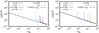
Figure S5: Local $g_{k}$-density of states $\rho_{g}(g_{k},E)$ for the quantity $g_{k}=(\cos(k_{x})-\cos(k_{y}))/2$ for different values of energies $E$/filling factors $n$ (see text for the definition). The dashed black line shows the analytical result $\rho_{g}(g_{k},E)=C_{1}(1-g_{k})^{-1}$ which is obtained for the exact separatrix case and if $1-g_{k}\ll 1$. Here the constant is given by $C_{1}=1/(2\pi^{2}\sqrt{a_{x}a_{y}})$ where $a_{x}=a_{y}=2$ for the NN model ($a_{x}=2.084$, $a_{y}=0.452$ for the HTC model) such that $C_{1}=0.0253303$ ($C_{1}=0.052198$). The values of $a_{x}$ and $a_{y}$ are obtained from the expansion $E_{1}({\bf k})=E_{1}(0,\pi)+\frac{1}{2}[a_{x}k_{x}^{2}-a_{y}(\pi-k_{y})^{2}]$ for $(k_{x},k_{y})$ being close to the separatrix point $(0,\pi)$ (see text for more details). The constant $C_{1}$ for the HTC model is roughly twice as large than the constant $C_{1}$ for the NN model showing that for the HTC model $g_{k}$ values close to unity are more likely. For the NN model (left panel) the green curve for the separatrix value $n=1$ extends numerically up to $(1-g_{k})\approx 10^{-10}$. For the HTC model (right panel) the blue curve for $n=0.7435$ extends numerically to $(1-g_{k})\approx 3\times 10^{-6}$; the curve for the precise separatrix value $n=0.743465958$ (not shown in the figure) extends numerically to very small values of $(1-g_{k})\approx 10^{-12}$ (if computed properly). The strong peak values at minimal values of $1-g_{k}=1-g_{\rm max}$ correspond to singularities of the type const.$/\sqrt{g_{\rm max}-g_{k}}$ and in this region the density coincides numerically very well with the analytical approximation (27) showing a crossover from a power law with exponent $-1/2$ (for $g_{\rm max}-g_{k}\ll 1-g_{\rm max}$) to a different power law with exponent $-1$ corresponding to the black dashed line (for $1-g_{\rm max}\ll g_{\rm max}-g_{k}\ll 1$). Note that due to the exchange symmetry between $k_{x}$ and $k_{y}$ the local $g_{k}$-density of states is symmetric : $\rho_{g}(g_{k},E)=\rho_{g}(-g_{k},E)$ and therefore this function is only shown for positive values of $g_{k}\geq 0$.

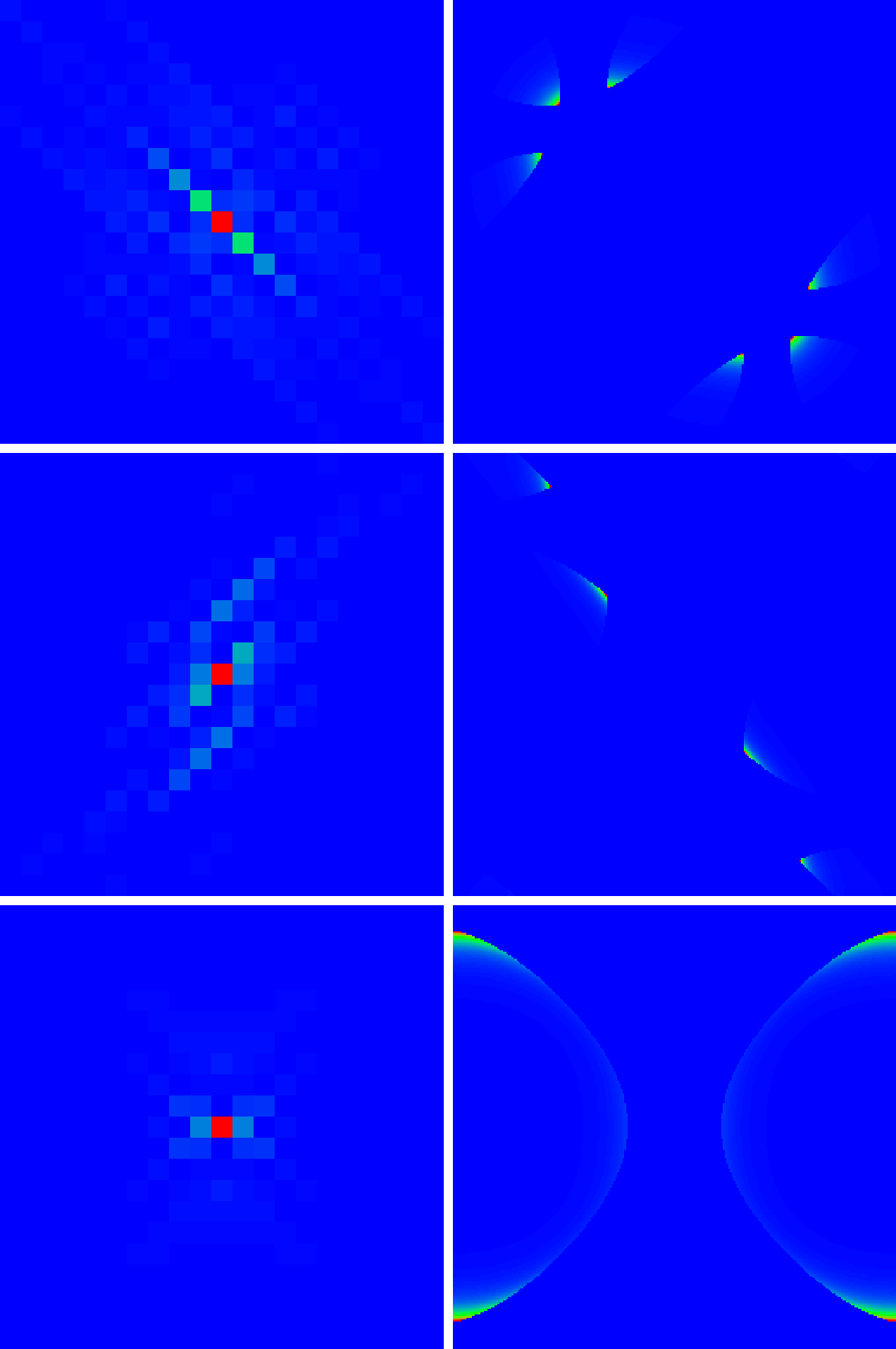
Figure S7: Ground state density plots for the Hubbard interaction, system size $N=256$, particle excitations, filling factor $n=0.84$ and three sectors ${\bf p}_{+}\neq 0$ (same values as in Fig. S6). Top (center, bottom) panels correspond to $U=-7$, ${\bf p}_{+}=2\pi(106,106)/256$ ($U=-8$, ${\bf p}_{+}=2\pi(52,174)/256$; $U=-6$, ${\bf p}_{+}=2\pi(27,256)/256$). Left panels show the ground state in $\Delta{\bf r}$-representation in a zoomed region with $-10\leq\Delta x,\Delta y\leq 10$ (color values outside the zoomed regions are blue) and right panels show the state in $\Delta{\bf p}$-representation (with $-\pi\leq\Delta p_{x,y}<\pi$). The two particle ground state energies $E_{\rm min}$ in units of the basic hopping matrix element are $-0.1337$ ($-0.1095$, $-0.2868$) for top (center, bottom) panels.

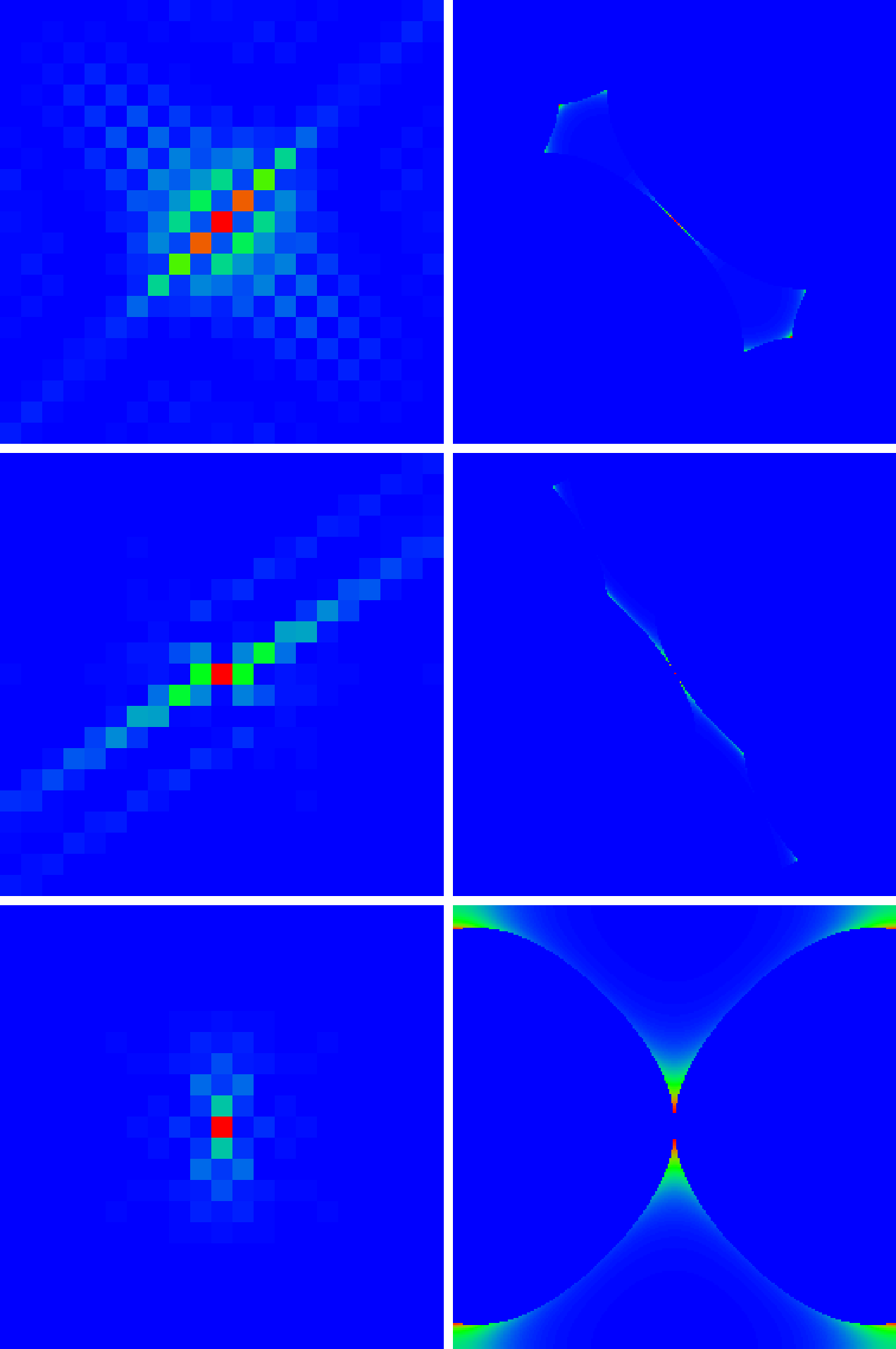
Figure S12: Ground state density plots for the Hubbard interaction, system size $N=256$, hole excitations, filling factor $n=0.84$ and three sectors ${\bf p}_{+}\neq 0$ (same values as in Fig. S11). Top (center, bottom) panels correspond to $U=-7$, ${\bf p}_{+}=2\pi(106,106)/256$ ($U=-8$, ${\bf p}_{+}=2\pi(52,174)/256$; $U=-6$, ${\bf p}_{+}=2\pi(27,256)/256$). Left panels show the ground state in $\Delta{\bf r}$-representation in a zoomed region with $-10\leq\Delta x,\Delta y\leq 10$ (color values outside the zoomed regions are blue) and right panels show the state in $\Delta{\bf p}$-representation (with $-\pi\leq\Delta p_{x,y}<\pi$). The two particle ground state energies $E_{\rm min})$ in units of the basic hopping matrix element $t$ are $-0.04761$ ($-0.05367$, $-0.3767$) for top (center, bottom) panels.

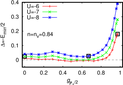
Figure S13: As Fig. 12 but for $n=n_{v}=0.84$ with three interaction values and the black square data points/states corresponding to Fig. S12.

Figure S16: Fermi surface for different filling factors as in Fig. 1 superimposed with color plots showing the regions of negative mass eigenvalues in classical phase space. Top (bottom) panels correspond to the NN model (HTC model). Left (right) panels correspond the smaller eigenvalue $\lambda_{2}$ (larger eigenvalue $\lambda_{1}$). Shown are the regions of negative values for these eigenvalues with colors yellow (cyan, blue) for strong (intermediate, close to 0) negative values. The regions of white color correspond to positive $\lambda_{1,2}$. The eigenvalues $\lambda_{1},\,\lambda_{2}$ as a function of the center of mass ${\bf p}_{+}/2={\bf p}$ are computed as the eigenvalues of the Hessian matrix obtained by expanding $E_{1p}({\bf p}_{+}/2-\Delta{\bf p})+E_{1p}({\bf p}_{+}/2+\Delta{\bf p})$ in $\Delta{\bf p}$ up to second order. Since $\lambda_{1}>\lambda_{2}$ the right panels show the regions where both eigenvalues are negative. The shown filling values $n$ in this figure actually correspond to the virtual filling $n_{v}=n$ as far as the superimposed color plot for the negative mass eigenvalues are concerned (since ${\bf p}_{+}/2={\bf p}$).

References

• (1) K.A. Müller, and J.G. Bednorz, Z. Phys. B: Condens. Matter 64, 189 (1986).
• (2) E. Dagotto, Rev. Mod. Phys. 66, 763 (1994).
• (3) B. Keimer, S.A. Kivelson, M.R. Norman, S. Uchida, and Z. Zaanen, Nature 518, 179 (2015).
• (4) C. Proust, and L. Taillefer, Annu. Rev. Condens. Matter Phys. 10, 409 (2019).
• (5) P.W. Anderson, Science 235, 1196 (1987).
• (6) V.J. Emery, Phys. Rev. Lett. 58, 2794 (1987).
• (7) V.J. Emery, and G. Reiter, Phys. Rev. B 38, 4547 (1988).
• (8) C.M. Varma, Solid State Commun. 62, 681 (1987).
• (9) Y.B. Gaididei, and V.M. Loktev, Phys. Status Solidi 147, 307 (1988).
• (10) R.S. Markiewicz, S. Sahrakorpi, M. Lindroos, H. Lin, and A. Bansil, Phys. Rev. B 72, 054519 (2005).
• (11) T. Das, R.S. Markiewicz, and A. Bansil, Adv. Phys. 63, 151 (2014)
• (12) R. Photopoulos, and R. Fresard, Ann. Phys. (Berlin) 1900177 (2019).
• (13) L. Cooper, Phys. Rev. 104, 1189 (1956).
• (14) K.M. Frahm, and D.L. Shepelyansky, Phys. Rev. Research 2, 023354 (2020).
• (15) K.M.Frahm, and D.L.Shepelyansky, Eur. Phys. J. B 94, 29 (2021).
• (16) I.M.Vishik, W.S.Lee, R.-H.He, M.Hashimoto, Z.Hussain, T.P.Devereaux, and Z.-X.Shen, New J. Phys. 12, 105008 (2010),
• (17) M.Hashimoto, I.M.Vishik, R.-H.He, T.P.Devereaux, and Z.-H.Shen, Nature Phys. 10, 483 (2014).
• (18) K.M. Frahm, and D.L. Shepelyansky, Phys. Rev. Lett. 79, 1833 (1997).
• (19) R.Comin et al., Science 343, 390 (2014).
• (20) K. von Arx et al., arXiv:2206.06695[cond-mat.supr-con] (2022).
• (21) M. Tinkham, (1996). Introduction to Superconductivity, Dover Publications. p. 63.
• (22) K.M. Frahm, and D.L. Shepelyansky, Available upon request: https://www.quantware.ups-tlse.fr/QWLIB/electronpairsforhtc/; Accessed September (2022)
• (23) W. Kohn, and J.M. Luttinger, Phys. Rev. Lett. 15, 524 (1976).
• (24) A.V. Chubukov, Phys. Rev. B 48, 1097 (1993).
• (25) F. Guinea, and B. Uchoa, Phys. Rev. B 86, 134521 (2012).