Borel summability of the $\mathbf{1/N}$ expansion
in quartic $\mathbf{\mathrm{O}(N)}$-vector models

Abstract

We consider a quartic $\mathrm{O}(N)$-vector model. Using the Loop Vertex Expansion, we prove the Borel summability in $1/N$ along the real axis of the partition function and of the connected correlations of the model. The Borel summability holds uniformly in the coupling constant, as long as the latter belongs to a cardioid like domain of the complex plane, avoiding the negative real axis.

1 Introduction

The Loop Vertex Expansion (LVE) was introduced by Rivasseau in 2007 [Riv07] as a new tool in constructive field theory in order to deal with matrix fields. It was then successfully applied to general tensor fields [Gur13, DR16, RVT18]. For a general exposition in zero dimensions, close to the topic of this article, see [Riv09]. The outcome of the LVE is an expression of the free energy, as well as the generating function of connected moments (or cumulants) as a sum over trees instead of connected graphs. As the number of trees increases only exponentially with the number of vertices and the contribution of each tree is exponentially bounded, the resulting series is convergent. The two ingredients of this expansion are the Hubbard–Stratonovich [Hub59, Str57] intermediate field representation and the Brydges-Kennedy–Abdesselam-Rivasseau (BKAR) formula [BK87, AR95].

In this paper we study the Borel summability in $1/N$ of the free energy and the cumulants of the quartic $\mathrm{O}(N)$-vector model in zero dimensions using the LVE (see Section 2 for the definition of the model). Note that here we are not interested in the pertubative expansion (the expansion at small coupling constant), which is well-understood for the quartic $\mathrm{O}(N)$-vector model and is Borel summable in $0$ dimensions [Riv07] and in $2$ dimensions [EMS74]. On the contrary, Borel summability in $1/N$ is less explored. The associated two-dimensional Euclidean quantum field theory was studied in [BR82], where the authors prove the Borel summability of the partition function and of the moments of the $\frac{g}{N}\mathinner{\!\left\lVert\phi\right\rVert}^{4}_{2}$ measure. But they discuss neither the free energy nor the cumulants. Passing between the two is rather non trivial as one needs to take a logarithm. The raison d’être of the LVE is to take this logarithm rigorously and uniformly in $N$. A related model, the spherical $\mathrm{O}(N)$ model (or non-linear $\sigma$-model), has been studied in [Kup80a, FMR82] where the authors showed that the partition function and the correlation functions at high enough temperature are Borel summable in $1/N$. However, contrary to the model we study here, the spherical $\mathrm{O}(N)$ model does not have any issues of convergence at large field as the field is restricted to belong to the sphere $\mathbb{S}^{N-1}$.

Techniques similar to the ones we use in this paper have been introduced in [GK15] for $N\times N$ matrices. However, only the Borel summability of the perturbative expansion in the coupling constant has been established in [GK15]: the status of the $1/N$ series has not been analyzed. The generalization of Borel summability results in $1/N$ to the case of matrices is not straightforward: contrary to the vector case, we do not have a representation of the partition function (with sources) in which $N$ is just a parameter. Consequently it has been impossible so far to prove that such functions can be extended to analytic functions in $1/N$ in some domain.

In this article the free energy and the generating function of cumulants of the quartic $\mathrm{O}(N)$ vector model are considered as functions of the coupling constant $g$ and of $1/N$. We look for the largest domain in the $(g,1/N)$-plane allowing their bivariate analytic continuation. After introducing the model in Section 2, we present both the main tools and the two main results in Section 3, namely the analyticity (Thm. 3.6) and the Borel summability (Thm. 3.8) domains of the free energy and the cumulants. We obtain that if $\lvert\arg g+\arg 1/N\rvert<3\pi/2$, the free energy and the cumulants are analytic in a cardioid shaped domain in $g$ and, for $\lvert\arg g\rvert<{\pi}$ they are Borel summable in $1/N$ along the real axis uniformly in $g$ for $g$ in a slightly smaller cardioid domain. The proofs of these theorems are presented in Sections 4 and 5, respectively. In order to keep this article self-contained, we recall BKAR formula in Lemma 3.5, but other useful tools also appear in the appendix.

Acknowledgements.

L.F. is supported by the EDPIF. R. G. and C.I.P-S. have been supported by the European Research Council (ERC) under the European Union’s Horizon 2020 research and innovation program (grant agreement No818066) and by the Deutsche Forschungsgemeinschaft (DFG, German Research Foundation) under Germany’s Excellence Strategy EXC-2181/1 - 390900948 (the Heidelberg STRUCTURES Cluster of Excellence).

2 The model and the partition function

Before introducing the model, let us adopt the following notation:

• We denote by $I_{n}$ the identity matrix on $\mathbb{R}^{n}$ and by $\mathbbm{1}_{n}$ the $n\times n$ matrix with all entries equal to $1$.

• Let $C\in M_{n}(\mathbb{R})$ be symmetric positive and $X,Y\in\mathbb{R}^{n}$. We write $\langle X,Y\rangle_{C}$ for $\sum_{1\leq i,j\leq n}X_{i}C_{ij}Y_{j}$. If $C=I_{n}$, we omit it. We denote $\langle X,X\rangle$ by $\mathinner{\!\left\lVert X\right\rVert}^{2}$. Whenever $X\in\mathbb{R}^{n}$ is the argument of a function $F\mathrel{\mathop{\mathchar 58\relax}}\mathbb{R}^{n}\rightarrow\mathbb{C}$, we write

  $$\langle\partial,\partial\rangle_{C}F(X)=\sum_{1\leq i,j\leq n}C_{ij}\frac{\partial^{2}F}{\partial{x_{i}}\partial{x_{j}}}(X)\;.$$

• Let $C\in M_{n}(\mathbb{R})$ be symmetric positive semi-definite. We denote by $\mu_{C}$ the centered Gaussian probability distribution of covariance $C$ on $\mathbb{R}^{n}$. Note that it exists and is unique (see appendix B.1) even if $C$ is degenerate.

• If $F\mathrel{\mathop{\mathchar 58\relax}}\mathbb{R}^{n}\rightarrow\mathbb{C}$, we denote $\mathbb{E}_{C}[F(X)]$ the expectation of $F$ with respect to $\mu_{C}$:

  $$\mathbb{E}_{C}[F(X)]=\int d\mu_{C}(X)F(X)=[e^{\frac{1}{2}\langle\partial,\partial\rangle_{C}}F(X)]_{X=0}\;.$$

• We write $a\lesssim b$ if there is a constant $K>0$ such that $a\leq Kb$. If we want to specify that $K$ depends on some parameter $\alpha$, we write $a\lesssim_{\alpha}b$.

• Throughout this paper, we denote $1/N$ by $\epsilon$ when promoted to a complex variable.

Let $N$ be a positive integer and $g\in\{z\in\mathbb{C}\mid\Re z>0\}$. The zero-dimensional quartic $\mathrm{O}(N)$-vector model is a probability distribution $\nu$ on $\mathbb{R}^{N}$ defined as a perturbed Gaussian distribution in the following way: denoting by $\mathbb{E}$ the expectation with respect to $\nu$, for all $F\mathrel{\mathop{\mathchar 58\relax}}\mathbb{R}^{N}\rightarrow\mathbb{C}$ $\nu$-mesurable, the expectation of $F$ is

$$\mathbb{E}[F(X)]=\frac{\mathbb{E}_{I_{N}}[e^{-\frac{g}{8N}\mathinner{\!\left\lVert X\right\rVert}^{4}}F(X)]}{\mathbb{E}_{I_{N}}[e^{-\frac{g}{8N}\mathinner{\!\left\lVert X\right\rVert}^{4}}]}\;.$$

The Fourier-Laplace transform of the measure, also known in the physics literature as the partition function with sources $J\in\mathbb{R}^{N}$, denoted $Z(g,1/N;J)$, is:

$$Z\big{(}g,\frac{1}{N};J\big{)}=\mathbb{E}_{I_{N}}[e^{-\frac{g}{8N}\mathinner{\!\left\lVert X\right\rVert}^{4}}]\,\mathbb{E}[e^{\sqrt{N}\langle J,X\rangle}]=\mathbb{E}_{I_{N}}[e^{-\frac{g}{8N}\mathinner{\!\left\lVert X\right\rVert}^{4}+\sqrt{N}\langle J,X\rangle}]\;.$$

In particular, the partition function of $\nu$, $Z(g,1/N;0)=\mathbb{E}_{I_{N}}[e^{-\frac{g}{8N}\mathinner{\!\left\lVert X\right\rVert}^{4}}]$, is the normalisation constant of that measure.

Remark 2.1.

Note that we have made a particular choice of scaling of the sources $J$ with $N$. This scaling ensures that all the cumulants (see below for details) are non-trivial in the large $N$ limit. In the absence of this scaling, in the large $N$ limit the $\mathrm{O}(N)$-vector model is a Gaussian model with a complicated covariance corresponding to the resummation of the dominant diagrams in the large $N$ limit, the so-called cactus diagrams.

From now on, we will switch to an integral notation, more adapted to the LVE, and more reminiscent of the functional integration in quantum field theory. In particular, in accordance to the usual notation of quantum field theory, we denote $\phi\in\mathbb{R}^{N}$ the random vector so that the partition function with sources rewrites:

$$Z\big{(}g,\frac{1}{N};J\big{)} =\int_{\mathbb{R}^{N}}\frac{d^{N}\phi}{(2\pi)^{N/2}}\;e^{-\frac{1}{2}\mathinner{\!\left\lVert\phi\right\rVert}^{2}-\frac{g}{8N}\mathinner{\!\left\lVert\phi\right\rVert}^{4}+\sqrt{N}\langle J,\phi\rangle}=\int d\mu_{I_{N}}(\phi)\;e^{-\frac{g}{8N}\mathinner{\!\left\lVert\phi\right\rVert}^{4}+\sqrt{N}\langle J,\phi\rangle}\;.$$ (1)

Our aim is to study the expansion in $1/N$ of the partition function and the cumulants of the measure $\nu$. At fixed $N\in\mathbb{Z}_{>0}$, the integral in eq. (1) is absolutely convergent iff $\Re g\geq 0$ and defines $Z(g,\tfrac{1}{N};J)$ as a holomorphic function of $g$ for all $g\in\{z\in\mathbb{C}\mid\Re z>0\}$.

In [Riv07] it was noted that performing a change of variables (known as the Hubbard-Stratonovich transformation, or intermediate field representation) one can obtain a convergent expansion for the logarithm of the partition function. We thus insert in eq. (1) the Hubbard-Stratonovich intermediate field representation ($\imath=\sqrt{-1}$):

$$e^{-\frac{x^{2}}{2}}={\frac{1}{\sqrt{2\pi}}}\int_{\mathbb{R}}dy\;e^{-\frac{y^{2}}{2}+\imath xy}=\int d\mu_{1}(y)\;e^{\imath xy}\;,$$

for the quartic interaction term, $x=\frac{1}{2}\sqrt{g/N}\mathinner{\!\left\lVert\phi\right\rVert}^{2}$ and obtain:

$$Z\big{(}g,\frac{1}{N};J\big{)} =\int d\mu_{{I}_{N}}(\phi)\int d\mu_{1}(\sigma)\;e^{\imath\frac{1}{2}\sqrt{g/N}\,\mathinner{\!\left\lVert\phi\right\rVert}^{2}\sigma+\sqrt{N}\langle J,\phi\rangle}$$

$$=\int d\mu_{1}(\sigma)\;e^{\frac{N}{2}\ln R(\sigma,g/N)+\frac{N}{2}R(\sigma,g/N)\,\mathinner{\!\left\lVert J\right\rVert}^{2}}$$

$$=\int d\mu_{\frac{1}{N}}(\sigma)\;e^{\frac{N}{2}\ln R(\sigma,g)+\frac{N}{2}R(\sigma,g)\,\mathinner{\!\left\lVert J\right\rVert}^{2}}$$

where $R\mathrel{\mathop{\mathchar 58\relax}}\mathbb{C}^{2}\setminus\{(\frac{1}{\imath\sqrt{z}},z)\mathrel{\mathrel{\mathop{\mathchar 58\relax}}}z\in\mathbb{C}^{*}\}\rightarrow\mathbb{C}$, $R(\sigma,z)={(1-\imath\sqrt{z}\sigma)}^{-1}$ is called the resolvent.

Remark 2.2.

This transformation renders the O($N$) invariance explicit: the partition function depends only on the norm of the sources.

We observe that, at fixed $N\in\mathbb{Z}_{>0}$, $Z$ can be analytically continued in $g$ to all $\mathbb{C}\setminus\mathbb{R}_{-}$. The intermediate field representation also makes $1/N$ an explicit parameter [Kup80] in an integral representation of $Z(g,1/N;J)$, contrary to eq. (1) where $N$ is also present implicitly in the dimension of the integral. One can then study the analyticity properties of $Z(g,1/N;J)$ seen as a function of the variable $\epsilon=1/N$ that, since we are interested in Borel summability along the positive real axis, we promote to $\mathrm{H}=\{z\in\mathbb{C}\mid\Re z>0\}$. We parameterize $\mathbb{C}^{*}$ as $\{(\lvert z\rvert,\alpha)\in\mathbb{R}_{+}^{*}\times(-\pi,\pi]\}$ and for $z=(\lvert z\rvert,\alpha)\in\mathbb{C}^{*}$, we write $\arg z=\alpha$, and we use the same parametrization for $\mathrm{H}=\{z\in\mathbb{C}^{*}\mid\lvert\arg z\rvert<\pi/2\}$. Regarding $g$, since it appears in a square root in the resolvent, it is wiser to take it to be an element of the Riemann surface of the square root, whose basic properties are recall hereafter:

Definition 2.3 (Riemann surface of the square root).

Let us denote by $\sqrt{\phantom{z}}$ the principal branch of the complex square root defined on $\mathbb{C}\setminus\mathbb{R}_{-}$. Let $\Sigma$ be the associated Riemann surface. We write $\sqrt[\sim]{\phantom{\omega}}$ for the analytic continuation of $\sqrt{\phantom{z}}$ to $\Sigma$. $\Sigma$ is a $2$-sheeted covering of $\mathbb{C}^{*}$ and can be parameterized as $\{(\lvert z\rvert,\alpha)\in\mathbb{R}_{+}^{*}\times(-2\pi,2\pi]\}$ and for $z=(\lvert z\rvert,\alpha)\in\Sigma$, we write $\operatorname{\widetilde{\arg}}z=\alpha$. Let $\mathrm{I}\mathrel{\mathop{\mathchar 58\relax}}z=(\lvert z\rvert,\alpha)\in\mathbb{C}\setminus\mathbb{R}_{-}\mapsto(\lvert z\rvert,\alpha)\in\Sigma$ be the canonical injection of $\mathbb{C}\setminus\mathbb{R}_{-}$ into $\Sigma$ and $\Pi$ be the projection of $\Sigma$ onto $\mathbb{C}^{*}$ namely $\Pi(\lvert z\rvert,\alpha)=\lvert z\rvert e^{\imath\alpha}$. The two sheets of $\Sigma$ correspond to the two possible determinations of the square root on $\mathbb{C}\setminus\mathbb{R}_{-}$ : for $z\in\Sigma$ such that $\operatorname{\widetilde{\arg}}z\in(-\pi,\pi)$, $\sqrt[\sim]{z}=\sqrt{\Pi z}$ and if $\operatorname{\widetilde{\arg}}z\in(-2\pi,-\pi)\cup(\pi,2\pi]$, $\sqrt[\sim]{z}=-\sqrt{\Pi z}$ (but note that $(\sqrt[\sim]{z})^{2}$ is always equal to $\Pi z$). We will denote by $\Sigma^{+}$ (resp. $\Sigma^{-}$) the sheet of $\Sigma$ corresponding to $\sqrt{\phantom{z}}$ (resp. to $-\sqrt{\phantom{z}}$), and we will also denote $\widetilde{R}(\sigma,z)\coloneqq(1-\imath\sigma\sqrt[\sim]{z})^{-1}$.

Therefore, from now on, the coupling constant $g$ is an element of $\Sigma$, and we aim to find the maximal domain of analyticity of the free energy and the cumulants as functions of $(g,\epsilon)\in\Sigma\times\mathrm{H}$. Since this will bring us to constantly deal with with the arguments of $g$ and $\epsilon$, in the rest of the article, we use the following convention:

$$\text{we will use indifferently $\operatorname{\widetilde{\arg}}g$ and $\varphi$, as well as $\arg\epsilon$ and $\theta$}.$$

At this point, partition function rewrites as

$$Z(g,\epsilon;J) =\int d\mu_{\epsilon}(\sigma)\;e^{\frac{1}{2\epsilon}\ln\widetilde{R}(\sigma,g)+\frac{1}{2\epsilon}\widetilde{R}(\sigma,g)\,\mathinner{\!\left\lVert J\right\rVert}^{2}}\,,$$

which enables to analytically continue it from $\mathrm{I}(\mathbb{R}_{+}^{*})\times\{1/N\mid N\in\mathbb{Z}_{>0}\}$ to $\mathrm{I}(\mathbb{C}\setminus\mathbb{R}_{-})\times\mathrm{H}$. In order to extend this continuation to some wider subdomain of $\Sigma\times\mathrm{H}$, for all $\psi\in(\theta-\pi/2,\theta+\pi/2)$ we define $Z_{\psi}(g,\epsilon;J)$ by

$$Z_{\psi}(g,\epsilon;J) =\int_{e^{\imath\frac{\psi}{2}}\mathbb{R}}\frac{d\sigma}{\sqrt{2\pi\epsilon}}\;e^{-\frac{\sigma^{2}}{2\epsilon}+\frac{1}{2\epsilon}\ln\widetilde{R}(\sigma,g)+\frac{1}{2\epsilon}\widetilde{R}(\sigma,g)\,\mathinner{\!\left\lVert J\right\rVert}^{2}}$$

$$=\int_{\mathbb{R}}\frac{d\sigma}{e^{-\imath\frac{\psi}{2}}\sqrt{2\pi\epsilon}}\;e^{-\frac{\sigma^{2}}{2\epsilon e^{-\imath\psi}}+\frac{1}{2\epsilon}\ln\widetilde{R}(\sigma e^{\imath\frac{\psi}{2}},g)+\frac{1}{2\epsilon}\widetilde{R}(\sigma e^{\imath\frac{\psi}{2}},g)\,\mathinner{\!\left\lVert J\right\rVert}^{2}}$$

$$=\int d\mu_{\epsilon e^{-\imath\psi}}(\sigma)\;e^{\frac{1}{2\epsilon}\ln\widetilde{R}(\sigma e^{\imath\frac{\psi}{2}},g)+\frac{1}{2\epsilon}\widetilde{R}(\sigma e^{\imath\frac{\psi}{2}},g)\,\mathinner{\!\left\lVert J\right\rVert}^{2}}\;.$$ (2)

The integral is convergent and, furthermore, $Z_{\psi}(g,\epsilon;J)=Z(g,\epsilon;J)$ is independent of $\psi$. Indeed, let $s_{g,\epsilon,J}\mathrel{\mathop{\mathchar 58\relax}}\sigma\in\mathbb{C}\mapsto\frac{1}{\sqrt{2\pi\epsilon}}\;e^{-\frac{\sigma^{2}}{2\epsilon}+\frac{1}{2\epsilon}\ln\widetilde{R}(\sigma,g)+\frac{1}{2\epsilon}\widetilde{R}(\sigma,g)\,\mathinner{\!\left\lVert J\right\rVert}^{2}}$ so that $Z_{\psi}(g,\epsilon;J)=\int_{\mathbb{R}}e^{\imath\frac{\psi}{2}}s_{g,\epsilon,J}(\sigma e^{\imath\frac{\psi}{2}})d\sigma$. We then have $\frac{d}{d\psi}Z_{\psi}(g,\epsilon;J)=\int_{\mathbb{R}}\frac{\imath}{2}e^{\imath\frac{\psi}{2}}d\sigma[s_{g,\epsilon,J}(\sigma e^{\imath\frac{\psi}{2}})+\sigma{s^{\prime}}_{g,\epsilon,J}(\sigma e^{\imath\frac{\psi}{2}})]=0$ by integration by part.

Before going to the analyticity domain of the free energy and the cumulants, for the sake of comparison, we note the following result:

Proposition 2.4.

The partition function with sources of the zero-dimensional $\mathrm{O}(N)$-vector model, $Z(g,\epsilon;J)$, can be analytically continued in $(g,\epsilon)$ from $\mathrm{I}(\mathbb{R}_{+}^{*})\times\{1/N\mid N\in\mathbb{Z}_{>0}\}$ to the following domain of $\Sigma\times\mathrm{H}$:

$$\mathfrak{B}=\Big{\{}(g,\epsilon)\in\Sigma\times\mathrm{H}\,\big{|}\,\operatorname{\widetilde{\arg}}g+\arg\epsilon\in\big{(}-\frac{3\pi}{2},\frac{3\pi}{2}\big{)}\Big{\}}.$$

Remark 2.5.

In the sequel, to prove Borel summability of the free energy or the cumulants of $\nu$, we will rely on the Nevanlinna-Sokal theorem [Sok79]. One important hypothesis of this theorem is analyticity in a disk tangent to the imaginary axis and centered at a positive real number. We call such a domain a Sokal disk, see remark A.2. Note that for $g\in\mathrm{I}(\mathbb{C}\setminus\mathbb{R}_{-})$, the analyticity domain in the $\epsilon$-plane of the partition function with sources contains indeed a Sokal disk as for all $\theta\in(-\pi/2,\pi/2)$ and $\varphi\in(-\pi,\pi)$, $\varphi+\theta\in(-3\pi/2,3\pi/2)$.

In order to prove Proposition 2.4, we need the following bound on the resolvent:

Lemma 2.6.

For all $(\sigma,g)\in\mathbb{C}^{*}\times\Sigma$,

$$\lvert\widetilde{R}(\sigma,g)\rvert\leq\frac{1}{\lvert\cos({\arg\sigma+\frac{1}{2}\operatorname{\widetilde{\arg}}{g}})\rvert}\,.$$ (3)

This bound is trivial for $\sqrt[\sim]{g}\sigma\in\imath\mathbb{R}$, which reflects the fact that the resolvent has a pole at $\sigma=1/\imath\sqrt[\sim]{g}$.

Proof.

Directly stems from $\lvert 1-\imath z\rvert\geq\lvert\cos\arg z\rvert$. ∎

Proof of Proposition 2.4.

We start with the intermediate field representation (2). Let $\mathfrak{H}_{\psi}$ be the following manifold:

$$\mathfrak{H}_{\psi}\coloneqq\big{\{}(\sigma,g,\epsilon)\in\mathbb{C}\times\Sigma\times\mathrm{H}\mid\sigma e^{\imath\frac{\psi}{2}}\sqrt[\sim]{g}\in\mathbb{C}\setminus\imath\mathbb{R}\big{\}}.$$

We let $f_{\psi}$ from $\mathfrak{H}_{\psi}$ to $\mathbb{C}$ be the integrand in eq. (2):

$$f_{\psi}(\sigma,g,\epsilon)=\frac{1}{e^{-\imath\frac{\psi}{2}}\sqrt{2\pi\epsilon}}e^{-\frac{\sigma^{2}}{2\epsilon e^{-\imath\psi}}+\frac{1}{2\epsilon}\ln\widetilde{R}(\sigma e^{\imath\frac{\psi}{2}},g)+\frac{1}{2\epsilon}\widetilde{R}(\sigma e^{\imath\frac{\psi}{2}},g)\,\mathinner{\!\left\lVert J\right\rVert}^{2}}.$$

$f_{\psi}$ is holomorphic on $\mathfrak{H}_{\psi}$ and $\int_{\mathbb{R}}f_{\psi}(\sigma,g,\epsilon)d\sigma$ coincides with (1) for $(g,\epsilon)\in\mathrm{I}(\mathbb{R}_{+}^{*})\times\{1/N\mid N\in\mathbb{Z}_{>0}\}$. For all $\sigma\in\mathbb{R}$, $(g,\epsilon)\mapsto f_{\psi}(\sigma,g,\epsilon)$ is holomorphic on $\mathfrak{A}_{\psi}\coloneqq\{(g,\epsilon)\in\Sigma\times\mathrm{H}\mid e^{\imath\frac{\psi}{2}}\sqrt[\sim]{g}\in\mathbb{C}\setminus\imath\mathbb{R}\}$, that has two connected components, namely

$$\mathfrak{A}_{\psi}^{+}=\big{\{}(g,\epsilon)\in\Sigma\times\mathrm{H}\mid\varphi\in(-\pi-\psi,\pi-\psi)\big{\}}$$ (4)

and $\mathfrak{A}_{\psi}^{-}=\{(g,\epsilon)\in\Sigma\times\mathrm{H}\mid\varphi\in(-2\pi,2\pi]\setminus(-\pi-\psi,\pi-\psi)\}$. Moreover as $\lvert\ln\widetilde{R}(\sigma e^{\imath\frac{\psi}{2}},g)\rvert\leq\lvert\ln\lvert\widetilde{R}(\sigma e^{\imath\frac{\psi}{2}},g)\rvert\rvert+\pi$, thanks to the bound (3), the integral of $f_{\psi}$ is absolutely convergent, uniformly in $g$ and $\epsilon$, on any compact of $\mathfrak{A}_{\psi}^{+}$. Thus, it defines an analytic continuation of $Z_{\psi}=Z$ to $\mathfrak{A}_{\psi}^{+}$. Therefore, $Z$ is analytic on $\bigcup_{\psi\in(\theta-\pi/2,\theta+\pi/2)}\mathfrak{A}_{\psi}^{+}=\mathfrak{B}$ which concludes the proof of Proposition 2.4. ∎

Remark 2.7.

This analytic continuation is the largest one that can be found thanks to the tilt of the contour of integration, since for $|\psi-\theta|\geq\pi/2$, the integral (2) becomes divergent.

Remark 2.8.

In order to clarify why the tilting of the contour was needed, consider the following. Suppose we are interested in the function $h\mathrel{\mathop{\mathchar 58\relax}}\{\Re z>0\}\rightarrow\mathbb{C},z\mapsto\int_{\mathbb{R}_{+}}e^{-zt}dt$ and ignore that $f(z)=1/z$. Clearly, $h$ is analytic on its domain of definition. We aim to analytically continue $h$ to some maximal domain. To this end, we observe that $h_{\psi}\mathrel{\mathop{\mathchar 58\relax}}z=\lvert z\rvert e^{\imath\alpha}\mapsto\int_{e^{\imath\psi}\mathbb{R}_{+}}e^{-zt}dt$ is analytic iff $\lvert\alpha+\psi\rvert<\pi/2$. Moreover, if $\lvert\psi\rvert<\pi$, the domains of analyticity of $h$ and $h_{\psi}$ overlap, and $h=h_{\psi}$ where they are both analytic. Thus $h_{\psi}$ is an analytic continuation of $f$ to a Riemann sheet. One needs to check whether this analytic continuation has a discontinuity at the real negative axis (in which case $0$ is a branch point) or a pole. In our case one gets a pole, but applying the same strategy to $z\mapsto\int_{\mathbb{R}}e^{-zt^{2}}dt$ one obtains a branch point of order $2$. We apply the same strategy to $Z$.

Our aim is to obtain similar results for the free energy and the cumulants. As such quantities depend on the logarithm of the partition function $Z$ and $Z$ has zeroes, they will not simply inherit the analyticity properties of $Z$: we expect that the domain of analyticity of $\ln Z$ is smaller than the one of $Z$. Since $Z(0,\epsilon;J)$ is non vanishing, for $g$ close to $0$, $Z(g,\epsilon;J)$ is non vanishing too. However, for $g$ real negative $Z$ is discontinuous and $g=0$ does not belong to the domain of analyticity of $Z$ or $\ln Z$. In order to identify some domain of analyticity of $\ln Z$ we will rewrite it as a uniformly convergent series of analytic functions. This series is indexed by trees and converges for a small enough coupling constant thereby defining $\ln Z$ in some domain. This is in contrast with the perturbative expansion which writes the partition function and the cumulants as divergent series.

The core of our arguments heavily relies on the Loop Vertex Expansion (LVE) [MR07, Riv07], which we now present.

3 The Loop Vertex Expansion of the cumulants

In this section, we perform the LVE of the cumulants defined hereafter:

Definition 3.1 (The rescaled cumulants).

For all $k\geq 1$, one defines the rescaled cumulant of order $2k$, $\mathfrak{K}^{2k}(g,\epsilon)$, by the following relation:

$$\left(\sum_{\pi\in P_{2}(2k)}\prod_{(a_{i},a_{j})\in\pi}\delta_{a_{i},a_{j}}\right)\mathfrak{K}^{2k}_{\psi}(g,\epsilon) \mathrel{\mathop{\mathchar 58\relax}}=\epsilon\frac{\partial^{2k}}{\partial_{J_{a_{1}}}...\partial_{J_{a_{2k}}}}\left.\ln{Z_{\psi}(g,\epsilon;J)}\right|_{J=0},$$ (5)

where $P_{2}(2k)$ is the set of pairings of $2k$ elements and let $\mathfrak{K}^{2k}(g,\epsilon)=\mathfrak{K}^{2k}_{\psi=0}(g,\epsilon)$.

This scaling is chosen as to have a well-defined large-$N$ limit and the advantage of using $\mathfrak{K}^{2k}$ over the RHS of (5) is that the former is manifestly O($N$) invariant. Since only $\mathfrak{K}^{2k}$ will appear below, we refer to them as the cumulants.

Before going to the Loop Vertex Expansion, let us introduce a few notations. First of all, in the following, we will denote by $\mathcal{T}_{n}$ be the set of all labelled trees with $n$ vertices. To a tree $T\in\mathcal{T}_{n}$, we associate the symmetric $n\times n$ matrix $W^{T}(u)$ with diagonal entries equal to $1$ and off diagonal ones $W_{ij}^{F}(u)=W_{ji}^{F}(u)=w_{ij}^{F}(u)$ as given by eq. (10). Then, the LVE is written in terms of

$$C^{n}_{k}=\big{\{}(i_{1},...,i_{k})\in\{1,...,n\}^{k}\mid\text{for all }a,b\in\{1,...,k\},a\neq b\Rightarrow i_{a}\neq i_{b}\big{\}}\;.$$

The notation comes from the fact that $C_{k}^{n}$ is the configuration space of $k$ particles on the discrete $n$-point space. With this notation at hand, the LVE allows us to express to cumulants as a sum over ciliated trees, for which we adopt the following convention:

$$\text{couples $(T,\mathfrak{c})$ made of a tree $T$ (with $n$ vertices) and \emph{cilia} $\mathfrak{c}\in C^{n}_{k}$ are denoted by $T_{\mathfrak{c}}$ }. \star$$ ()

For $i\in\{1,...,n\}$, we also denote $d_{i}(T_{\mathfrak{c}})=c(i)+d_{i}(T)$ with $c(i)=\textbf{1}_{i\in\mathfrak{c}}$ the coordination (or degree) of the vertex $i$ in $T_{\mathfrak{c}}$ including the cilia. The Loop Vertex expansion of the cumulants is given by the following proposition:

Proposition 3.2 (Loop Vertex expansion of the cumulants).

For all $1\leq k\leq n$ and $\psi\in(\theta-\pi/2,\theta+\pi/2)$, the cumulants are given by the series

$$\mathfrak{K}_{\psi}^{2k}(g,\epsilon)=2^{k-1}\sum_{n\geq k}\frac{1}{n!}{\left(\frac{-\Pi g}{2}\right)}^{n-1}\\ \times\sum_{T_{\mathfrak{c}}\in\mathcal{T}_{n}\times C^{n}_{k}}\int du_{T}\int d\mu_{\epsilon e^{-\imath\psi}W^{T}(u)}(\sigma)\bigg{\{}\prod_{i=1}^{n}(d_{i}(T_{\mathfrak{c}})-1)!\,\widetilde{R}^{d_{i}(T_{\mathfrak{c}})}(\sigma^{(i)}e^{\imath\frac{\psi}{2}},g)\bigg{\}}\;,$$

for all $(g,\epsilon)\in\Sigma\times\mathrm{H}$ such that it converges (in particular for $(g,\epsilon)\in\mathrm{I}(\mathbb{R}_{+}^{*})\times\mathbb{R}_{+}^{*}$).

Proof.

To perform the LVE, we first expand the partition function with sources as expressed in eq. (2). From now on, we fix $\psi\in(\theta-\pi/2,\theta+\pi/2)$ and for $(g,\epsilon)\in\mathfrak{B}$ we start from:

$$Z_{\psi}(g,\epsilon;J) =\int d\mu_{\epsilon e^{-\imath\psi}}(\sigma)\;e^{\frac{1}{2\epsilon}\ln\widetilde{R}(\sigma e^{\imath\frac{\psi}{2}},g)+\frac{1}{2\epsilon}\widetilde{R}(\sigma e^{\imath\frac{\psi}{2}},g)\,\mathinner{\!\left\lVert J\right\rVert}^{2}}\,.$$

We expand the exponential inside the integral and, using Fubbini’s theorem, we exchange the sum and the integral to obtain:

$$Z_{\psi}(g,\epsilon;J)=\sum_{n=0}^{\infty}\frac{1}{(2\epsilon)^{n}n!}\int d\mu_{\epsilon e^{-\imath\psi}}(\sigma)\big{[}\ln\widetilde{R}(\sigma e^{\imath\frac{\psi}{2}},g)+\widetilde{R}(\sigma e^{\imath\frac{\psi}{2}},g)\mathinner{\!\left\lVert J\right\rVert}^{2}\big{]}^{n}\;.$$ (6)

The use of Fubbini’s theorem is justified by the following lemma:

Lemma 3.3.

Let $a\in(0,1/2]$, $(g,\epsilon)\in\Sigma\times\mathrm{H}$ and $\psi\in(\theta-\pi/2,\theta+\pi/2)$. Then, if $(g,\epsilon)\in\mathfrak{A}^{+}_{\psi}$ (see eq. 4), there exist two non negative reals $C_{1},C_{2}$ independent of $\lvert g\rvert$ and $\lvert\epsilon\rvert$ such that for $n$ large enough:

$$A_{n}\mathrel{\mathop{\mathchar 58\relax}}=\frac{1}{(2\lvert\epsilon\rvert)^{n}n!}\bigg{|}\int d\mu_{\epsilon e^{-\imath\psi}}(\sigma)\big{[}{\ln\widetilde{R}(\sigma e^{\imath\frac{\psi}{2}},g)+\widetilde{R}(\sigma e^{\imath\frac{\psi}{2}},g)\mathinner{\!\left\lVert J\right\rVert}^{2}}\big{]}^{n}\bigg{|}\leq\frac{C_{1}^{n}}{\lvert\epsilon\rvert^{n}n!}+\frac{C_{2}^{n}\lvert g\rvert^{an}}{{(\lvert\epsilon\rvert^{n}n!)}^{(1-a)}}\,.$$

In particular, at fixed $\psi\in(\theta-\pi/2,\theta+\pi/2)$, the sum of the $A_{n}$’s has infinite radius of convergence in both $\lvert g\rvert$ and $1/\lvert\epsilon\rvert$ for all $(g,\epsilon)\in\mathfrak{A}_{\psi}^{+}$.

Proof.

It is convenient to perform the change of variable $\sigma\rightarrow\sigma\sqrt{\lvert g\rvert}$ so that $A_{n}$ rewrites:

$$\frac{1}{(2\lvert\epsilon\rvert)^{n}n!}\bigg{|}\int d\mu_{\lvert g\rvert\epsilon e^{-\imath\psi}}(\sigma)[\ln\widetilde{R}(\sigma e^{\imath\frac{\psi}{2}},\frac{g}{\lvert g\rvert})+\widetilde{R}(\sigma e^{\imath\frac{\psi}{2}},\frac{g}{\lvert g\rvert})\mathinner{\!\left\lVert J\right\rVert}^{2}]^{n}\bigg{|}.$$

Then, thanks to the bound in eq. (3), if $\lvert\psi+\varphi\rvert<\pi$, $\lvert\widetilde{R}(\sigma e^{\imath\frac{\psi}{2}},\frac{g}{\lvert g\rvert})\rvert\cdot\mathinner{\!\left\lVert J\right\rVert}^{2}\leq\frac{\mathinner{\!\left\lVert J\right\rVert}^{2}}{\cos{(\frac{\psi+\varphi}{2})}}$. Furthermore:

$$\big{|}{\ln{\widetilde{R}(\sigma e^{\imath\frac{\psi}{2}},\frac{g}{\lvert g\rvert})}}\big{|}\leq\big{[}\big{(}-\frac{1}{2}\ln\lvert\widetilde{R}^{-2}(\sigma e^{\imath\frac{\psi}{2}},\frac{g}{\lvert g\rvert})\rvert\big{)}^{2}+\pi^{2}\big{]}^{1/2}.$$

Then, using $\lvert\widetilde{R}^{-2}(\sigma e^{\imath\frac{\psi}{2}},\frac{g}{\lvert g\rvert})\rvert=1+2\sin{\frac{\psi+\varphi}{2}}\lvert\sigma\rvert+\sigma^{2}\leq(1+\lvert\sigma\rvert)^{2}$, we get $\ln{\lvert\widetilde{R}^{-2}(\sigma e^{\imath\frac{\psi}{2}},\frac{g}{\lvert g\rvert})\rvert}\leq\ln{(1+\lvert\sigma\rvert)^{2}}\leq 2(1+\lvert\sigma\rvert)^{2a}$ for $0<a<1/2$ implying $|{\ln{\widetilde{R}(\sigma e^{\imath\frac{\psi}{2}},\frac{g}{\lvert g\rvert})}}|\leq\sqrt{(1+\lvert\sigma\rvert)^{4a}+\pi^{2}}\leq(1+\lvert\sigma\rvert)^{2a}+\pi$ as $\pi>1$ so that:

$$A_{n} \leq\frac{1}{(2\lvert\epsilon\rvert)^{n}n!\sqrt{\cos(\psi-\theta)}}\int d\mu_{\frac{\lvert g\epsilon\rvert}{\cos(\psi-\theta)}}(\sigma)\big{[}(1+\lvert\sigma\rvert)^{2a}+\pi+\mathinner{\!\left\lVert J\right\rVert}^{2}\cos^{-1}{(\frac{\psi+\varphi}{2})}\big{]}^{n}$$

$$\leq\frac{1}{(2\lvert\epsilon\rvert)^{n}n!\sqrt{\cos(\psi-\theta)}}\int d\mu_{\frac{\lvert g\epsilon\rvert}{\cos(\psi-\theta)}}(\sigma)\sum_{k=0}^{n}\binom{n}{k}(1+\lvert\sigma\rvert)^{2ak}\big{[}\pi+\mathinner{\!\left\lVert J\right\rVert}^{2}\cos^{-1}{(\frac{\psi+\varphi}{2})}\big{]}^{n-k}$$

$$\leq\frac{\big{[}\pi+\mathinner{\!\left\lVert J\right\rVert}^{2}\cos^{-1}{(\frac{\psi+\varphi}{2})}\big{]}^{n}}{\lvert\epsilon\rvert^{n}n!\sqrt{\cos(\psi-\theta)}}\int d\mu_{\frac{\lvert g\epsilon\rvert}{\cos(\psi-\theta)}}(\sigma)(1+\lvert\sigma\rvert)^{2an}\,,$$

where we used the fact that $\pi+\mathinner{\!\left\lVert J\right\rVert}^{2}\cos^{-1}{(\frac{\psi+\varphi}{2})}$ and $1+\lvert\sigma\rvert$ are greater than one. At this stage, rewriting:

$$\int d\mu_{\frac{\lvert g\epsilon\rvert}{\cos(\psi-\theta)}}(\sigma)(1+\lvert\sigma\rvert)^{2an} =\int_{\lvert\sigma\rvert<1}d\mu_{\frac{\lvert g\epsilon\rvert}{\cos(\psi-\theta)}}(\sigma)(1+\lvert\sigma\rvert)^{2an}+\int_{\lvert\sigma\rvert>1}d\mu_{\frac{\lvert g\epsilon\rvert}{\cos(\psi-\theta)}}(\sigma)(1+\lvert\sigma\rvert)^{2an}$$

$$\leq\int_{\lvert\sigma\rvert<1}d\mu_{\frac{\lvert g\epsilon\rvert}{\cos(\psi-\theta)}}(\sigma)2^{2an}+\int_{\lvert\sigma\rvert>1}d\mu_{\frac{\lvert g\epsilon\rvert}{\cos(\psi-\theta)}}(\sigma)(2\lvert\sigma\rvert)^{2an}$$

$$\leq 2^{2an}\bigg{(}\int_{\mathbb{R}}d\mu_{\frac{\lvert g\epsilon\rvert}{\cos(\psi-\theta)}}(\sigma)+\int_{\mathbb{R}}d\mu_{\frac{\lvert g\epsilon\rvert}{\cos(\psi-\theta)}}(\sigma)\lvert\sigma\rvert^{2an}\bigg{)}$$

$$\leq 4^{an}\bigg{(}1+\frac{1}{2\sqrt{\pi}}\big{[}\frac{\cos{(\psi-\theta)}}{2\lvert g\epsilon\rvert}\big{]}^{1/2}\int_{\mathbb{R}_{+}}e^{-\cos{(\psi-\theta)}\frac{t}{2\lvert g\epsilon\rvert}}t^{an-1/2}dt\bigg{)}$$

$$\leq 4^{an}\bigg{(}1+\frac{1}{2\sqrt{\pi}}\big{[}\frac{2\lvert g\epsilon\rvert}{\cos{(\psi-\theta)}}\big{]}^{an}\Gamma\big{(}an+\frac{1}{2}\big{)}\bigg{)}\,,$$

and using the asymptotic of the gamma function we get $A_{n}\leq\frac{C_{1}^{n}}{\lvert\epsilon\rvert^{n}n!}+\frac{C_{2}^{n}\lvert g\rvert^{an}}{{(\lvert\epsilon\rvert^{n}n!)}^{(1-a)}}$.∎

We now use the copies trick as stated in Lemma B.5 (see Appendix B.3 for the proof). With our integral notations, Lemma B.5 rewrites:

Lemma 3.4 (The copies trick).

Let $n$ be a positive integer, $z\in\mathbb{C}$ with $\Re z>0$ and $F\in L^{n}(\mathbb{R},\mu_{\lvert z\rvert^{2}/\Re z})$ a $\mathbb{C}$-valued function. Then $F^{\otimes n}\mathrel{\mathop{\mathchar 58\relax}}\mathbb{R}^{n}\to\mathbb{C}$, $X=(X_{i})_{1\leq i\leq n}\mapsto\prod_{1=n}^{n}F(X_{i})$ is in $L^{1}(\mathbb{R}^{n},\mu_{{\lvert z\rvert^{2}\mathbbm{1}_{n}/\Re z}})$ and furthermore we have:

$$\int d\mu_{z}(x)F^{n}(x)=\int d\mu_{z\mathbbm{1}_{n}}(X)F^{\otimes n}(X)=\int d\mu_{z\mathbbm{1}_{n}}(X)\prod_{i=1}^{n}F(X_{i})\;.$$ (7)

This lemma produces for an integration variable $\sigma$, $n$ variables of integration that we call the copies of $\sigma$ and that we denote by $(\sigma^{(i)})_{1\leq i\leq n}$, where we use parenthesis to avoid the confusion with the O($N$) indices. With this notation, using eq. (7) in eq. (6) we obtain that:

$$Z_{\psi}(g,\epsilon;J)=\sum_{n\geq 0}\frac{1}{(2\epsilon)^{n}n!}\int d\mu_{\epsilon e^{-\imath\psi}\mathbbm{1}_{n}}(\sigma)\prod_{i=1}^{n}\bigg{\{}\ln\widetilde{R}(\sigma^{(i)}e^{\imath\frac{\psi}{2}},g)+\widetilde{R}(\sigma^{(i)}e^{\imath\frac{\psi}{2}},g)\mathinner{\!\left\lVert J\right\rVert}^{2}\bigg{\}}$$ (8)

$$={} \sum_{n\geq 0}\frac{1}{(2\epsilon)^{n}n!}\left[\exp\Big{(}\frac{\epsilon e^{-\imath\psi}}{2}\langle\partial,\partial\rangle_{X(x)}\Big{)}\prod_{i=1}^{n}\bigg{\{}\ln\widetilde{R}(\sigma^{(i)}e^{\imath\frac{\psi}{2}},g)+\widetilde{R}(\sigma^{(i)}e^{\imath\frac{\psi}{2}},g)\mathinner{\!\left\lVert J\right\rVert}^{2}\bigg{\}}\right]_{\sigma^{(i)}=0,x_{ij}=1}\,,$$

where $[X(x)]_{ii}=1$ and $[X(x)]_{ij}=x_{ij}$ for $i\neq j$.

We now rewrite the above expansion as a sum indexed by forests over labelled vertices of analytic functions and consequently its logarithm as a sum indexed by trees over labelled vertices of analytic functions. The crucial point is that at order $n$ the number of such trees is of order $O(1)^{n}n!$, much less than the number of Feynman diagrams which is of order $O(1)^{n}(2n)!$, and the expansion is convergent.

This rewriting is obtained thanks to the BKAR formula [BK87, AR95], which will be applied to the $x=(x_{ij})$ parameters.

Lemma 3.5 (BKAR formula).

Let $f\mathrel{\mathop{\mathchar 58\relax}}\mathbb{R}^{\frac{n(n-1)}{2}}\rightarrow{\mathbb{C}}$ be a smooth function. If $x\in\mathbb{R}^{\frac{n(n-1)}{2}}$, we denote its components by $x_{ij}$ for $i,j=1,2,\dots,n$, $i<j$. Let $F$ be a forest with vertex set $V(F)=\{1,2,\dotsc,n\}$. If there is an edge between vertices $i$ and $j$ ($i<j$), we write $(i,j)\in E(F)$. If both $i$ and $j$ belong to the same connected component of $F$, we let $P_{i\leftrightarrow j}^{F}$ stand for the unique path in $F$ between $i$ and $j$. Then we have:

$$f(x)\big{|}_{x=\mathbf{1}}=\sum_{F\in\mathcal{F}_{n}}\Big{(}\prod_{(i,j)\in E(F)}\int_{0}^{1}du_{ij}\Big{)}\,\frac{\partial^{|E(F)|}f(x)}{\prod_{(l,m)\in E(F)}\partial x_{lm}}\bigg{|}_{x=w^{F}}\,,$$ (9)

where $\mathbf{1}$ is the $\frac{n(n-1)}{2}$-vector with all the components equal to $1$, $\mathcal{F}_{n}$ is the set of all forests with $n$ labelled vertices, $|E(F)|$ is the number of edges of $F$, and $w^{F}\in\mathbb{R}^{\frac{n(n-1)}{2}}$ is given by:

$$w^{F}_{ij}\coloneqq\begin{cases}\inf_{(k,l)\in P_{i\leftrightarrow j}^{F}}u_{kl}&\text{if $i$ and $j$ belong to the same component of $F$,}\\ 0&\text{otherwise.}\end{cases}$$ (10)

Notice that $\prod_{(a,b)\in E(F)}\partial_{x_{ab}}={\epsilon}^{\lvert E(F)\rvert}e^{-\imath\psi\lvert E(F)\rvert}\prod_{(ab)\in E(F)}\partial_{\sigma^{(a)}}\partial_{\sigma^{(b)}}$ when acting on the quantity in square brackets in (8). Thus, by the BKAR formula (9), the partition function with sources rewrites as

$$Z_{\psi}(g,\epsilon;J)=\sum_{n\geq 0}\frac{1}{(2\epsilon)^{n}n!}\sum_{F\in\mathcal{F}_{n}}\int du_{F}\int d\mu_{\epsilon e^{-\imath\psi}W^{F}(u)}(\sigma){\epsilon}^{\lvert E(F)\rvert}e^{-\imath\psi\lvert E(F)\rvert}\\ \times\prod_{(a,b)\in E(F)}\partial_{\sigma^{(a)}}\partial_{\sigma^{(b)}}\prod_{i=1}^{n}\bigg{\{}\ln\widetilde{R}(\sigma^{(i)}e^{\imath\frac{\psi}{2}},g)+\widetilde{R}(\sigma^{(i)}e^{\imath\frac{\psi}{2}},g)\mathinner{\!\left\lVert J\right\rVert}^{2}\bigg{\}}\;,$$

where we recall that for $F\in\mathcal{F}_{n}$, $W^{F}(u)$ is the symmetric $n\times n$ matrix with diagonal entries equal to $1$ and off diagonal ones $W_{ij}^{F}(u)=W_{ji}^{F}(u)=w_{ij}^{F}(u)$ as given by eq. (10), $du_{F}=\prod_{(ij)\in{F}}\int_{0}^{1}du_{ij}$. The matrix $W^{F}(u)$ is positive.

The logarithm of the partition function with sources is the generating function of the cumulants. Now that the partition function with sources is expressed as a sum over forests with the amplitude of a forest factorizing over the trees of this forest, its logarithm writes as a sum over trees. As $\lvert E(T)\rvert=|V(T)|-1$, we get:

$$\epsilon\ln{Z}_{\psi}(g,\epsilon;J)=\sum_{n\geq 1}\frac{e^{-\imath(n-1)\psi}}{2^{n}n!}\sum_{T\in\mathcal{T}_{n}}\int du_{T}\int d\mu_{\epsilon e^{-\imath\psi}W^{T}(u)}(\sigma)\prod_{(a,b)\in E(T)}\partial_{\sigma^{(a)}}\partial_{\sigma^{(b)}}\sum_{k=0}^{n}\frac{{\mathinner{\!\left\lVert J\right\rVert}^{2k}}}{k!}\\ \times\sum_{\begin{subarray}{c}1\leq i_{1},...,i_{k}\leq n\\ a\neq b\Rightarrow i_{a}\neq i_{b}\end{subarray}}\prod_{c=1}^{k}\widetilde{R}(\sigma^{(i_{c})}e^{\imath\frac{\psi}{2}},g)\prod_{j\neq i_{1},...,i_{k}}\ln{\widetilde{R}(\sigma^{(j)}e^{\imath\frac{\psi}{2}},g})\,,$$

were we recall that $\mathcal{T}_{n}$ stands for the set of all trees with $n$ labelled vertices. At this stage, we can rewrite the sum above in terms of $C^{n}_{k}$ and of ciliated trees (recall the convention ($\star$ ‣ 3)). Indeed, repeatedly using the fact that $\partial_{\sigma}^{k}\ln\widetilde{R}(\sigma e^{\imath\frac{\psi}{2}},g)={(\imath e^{\imath\frac{\psi}{2}}\sqrt[\sim]{g})}^{k}(k-1)!\,\widetilde{R}^{k}(\sigma e^{\imath\frac{\psi}{2}},g)$, $\partial_{\sigma}^{k}\widetilde{R}(\sigma e^{\imath\frac{\psi}{2}},g)={(\imath e^{\imath\frac{\psi}{2}}\sqrt[\sim]{g})}^{k}k!\,\widetilde{R}^{k+1}(\sigma e^{\imath\frac{\psi}{2}},g)$, $(\sqrt[\sim]{g})^{2}=\Pi g$ and the combinatorial identity $\sum_{i}d_{i}=2(n-1)$, the logarithm of the partition function with sources becomes:

$$\epsilon\ln{Z}_{\psi}(g,\epsilon;J)=\frac{1}{2}\sum_{n\geq 1}\frac{1}{n!}{\left(\frac{-\Pi g}{2}\right)}^{n-1}\sum_{k=0}^{n}\frac{\mathinner{\!\left\lVert J\right\rVert}^{2k}}{k!}\sum_{T_{\mathfrak{c}}\in\mathcal{T}_{n}\times C^{n}_{k}}\int du_{T}\int d\mu_{\epsilon e^{-\imath\psi}W^{T}(u)}(\sigma)\\ \times\prod_{i=1}^{n}\big{\{}(d_{i}(T_{\mathfrak{c}})-1)!\,\widetilde{R}^{d_{i}(T_{\mathfrak{c}})}(\sigma^{(i)}e^{\imath\frac{\psi}{2}},g)\big{\}}.$$

Using $\frac{\partial^{2k}}{\partial_{J_{a_{1}}}...\partial_{J_{a_{2k}}}}\mathinner{\!\left\lVert J\right\rVert}^{2k}=2^{k}k!\sum_{\pi\in P_{2}(2k)}\prod_{(a_{i},a_{j})\in\pi}\delta_{a_{i},a_{j}}$, we obtain the following expression, that holds true as long as both the individual integrals converge and the overall series is convergent (recall that with the convention ($\star$ ‣ 3), $T$ is the tree $T_{\mathfrak{c}}$ without cilia):

$$\mathfrak{K}_{\psi}^{2k}(g,\epsilon)=2^{k-1}\sum_{n\geq k}\frac{1}{n!}{\left(\frac{-\Pi g}{2}\right)}^{n-1}\\ \times\sum_{T_{\mathfrak{c}}\in\mathcal{T}_{n}\times C^{n}_{k}}\int du_{T}\int d\mu_{\epsilon e^{-\imath\psi}W^{T}(u)}(\sigma)\bigg{\{}\prod_{i=1}^{n}(d_{i}(T_{\mathfrak{c}})-1)!\,\widetilde{R}^{d_{i}(T_{\mathfrak{c}})}(\sigma^{(i)}e^{\imath\frac{\psi}{2}},g)\bigg{\}}\;,$$ (11)

which concludes the proof. ∎

Our first main theorem concerns the domain in $(g,\epsilon)$ in which the rescaled cumulants are analytic in both variables.

Theorem 3.6 (Main Theorem 1: Analyticity).

For all $k\geq 1$, the cumulant of order $2k$ of the quartic $\mathrm{O}(N)$-vector model, $\mathfrak{K}^{2k}(g,\epsilon)$, as expressed by the series (11), is analytic in $g$ and $\epsilon$ on the domain $\mathfrak{C}$ consisting in all the couples $(g,\epsilon)\in\Sigma\times\mathrm{H}$ such that there exists $\psi\in(-\pi,\pi)$ for which the following inequalities hold:

$$\lvert g\rvert <\frac{1}{4}(1+\cos{(\operatorname{\widetilde{\arg}}g+\psi)})\sqrt{\cos{(\psi-\arg\epsilon)}}\;,$$ (12a)

$$\lvert\operatorname{\widetilde{\arg}}g+\psi\rvert <\pi\;,$$ (12b)

$$\lvert\psi-\arg\epsilon\rvert <\frac{\pi}{2}\;.$$ (12c)

The proof of this theorem is given is Section 4.

Corollary 3.7 (Domain as a Riemann sheet).

At fixed $g\in\Sigma$, the domain of analyticity in $\epsilon$ is independent of its modulus, and contains all $\epsilon\in\mathrm{H}$ such that $-3\pi/2-\operatorname{\widetilde{\arg}}g<\arg\epsilon<3\pi/2-\operatorname{\widetilde{\arg}}g$. In particular, for all $\lvert\epsilon\rvert\geq 0$, $\theta\in(-\pi/2,\pi/2)$, and $\varphi\in(-\pi,\pi)$, $((\lvert g\rvert,\varphi),\lvert\epsilon\rvert e^{\imath\theta})$ belongs to $\mathfrak{C}$ if $\lvert g\rvert$ is small enough (see discussion in Remark 3.10 for how small “small enough” is) and for such $g$, $\mathfrak{C}$ includes a Sokal disk in the $\epsilon$-plane (see Remark A.2) of an arbitrary, positive radius.

Proof.

The two conditions on $\varphi$ and $\theta$ read:

$$\begin{cases}\lvert\varphi+\psi\rvert<\pi\\ \lvert\psi-\theta\rvert<\frac{\pi}{2}\end{cases}\Leftrightarrow\begin{cases}-\pi<\varphi+\psi<\pi\\ -\frac{\pi}{2}<\theta-\psi<\frac{\pi}{2}\end{cases}\Rightarrow-\frac{3\pi}{2}<\varphi+\theta<\frac{3\pi}{2}\Leftrightarrow-\frac{3\pi}{2}-\varphi<\theta<\frac{3\pi}{2}-\varphi\;,$$

and observing that $\bigcap_{\varphi\in(-\pi,\pi)}(-3\pi/2-\varphi,3\pi/2-\varphi)=(-\pi/2,\pi/2)$ we conclude. ∎

Theorem 3.8 (Main Theorem 2: Borel summability).

For small $\alpha>0$ we define the subdomain $\mathfrak{C}_{\alpha}$ of $\mathfrak{C}$ made of all couples $(g,\epsilon)\in\Sigma\times\mathrm{H}$ such that there exists $\psi\in(-\pi,\pi)$ for which the following inequalities hold:

$$\lvert g\rvert <\frac{1}{4}(1+\cos{(\operatorname{\widetilde{\arg}}g+\psi)})\sqrt{\cos{(\psi-\arg\epsilon)}}\,(1-\alpha),$$ (13a)

$$\lvert\operatorname{\widetilde{\arg}}g+\psi\rvert <\pi\,(1-\alpha),$$ (13b)

$$\lvert\psi-\arg\epsilon\rvert <\frac{\pi}{2}\,(1-\alpha).$$ (13c)

For all $k\geq 1$, the rescaled cumulant of order $2k$ of the $\mathrm{O}(N)$-vector model $\mathfrak{K}^{2k}(g,\epsilon)$ is Borel summable in $\epsilon$ along the positive real axis for $g$ inside a non trivial domain (see Remark 3.10) and for $g$ inside this domain they can be computed as the Borel sum of their large $N$ expansion.

Proof.

The proof of this theorem follows from Corollary 3.7 and from the following lemma, proven in Section 5:

Lemma 3.9.

For small $\alpha>0$, for all $k\geq 1$ and for all $(g,\epsilon)\in\mathfrak{C}_{\alpha}$, there exists two constants $C_{\alpha}>0$ and $K_{\alpha}>0$ independent of $g$ and $\epsilon$ but depending on $\alpha$ such that the Taylor rest term of order $q$ in the $\epsilon$ expansion of the cumulant, denoted by $R^{2k}_{q}(g,\epsilon)$ (see eq. (17) for a closed expression of this rest term), obeys the following bound for $q$ large enough:

$$\lvert R^{2k}_{q}(g,\epsilon)\rvert\lesssim_{k}C_{\alpha}K_{\alpha}^{q}{\lvert\epsilon\rvert}^{q}q!\;.$$

This bound together with Corollary 3.7 prove that the cumulants verify the hypotheses of the Nevanlinna Sokal theorem [Sok79] uniformly in $g$ (for completeness we recall the relevant version of this theorem in Thm. A.1). ∎

Remark 3.10.

We now wish to visualize the domain $\mathfrak{C}\subset\Sigma\times\mathrm{H}$ (or $\mathfrak{C}_{\alpha}$ for $\alpha\to 0$). Let us go to the $\mathbb{C}$-plane of $\Pi g$ and look for the curve $\rho(\varphi)$ defined by:

$$\varphi\mapsto\rho(\varphi)\mathrel{\mathop{\mathchar 58\relax}}=\sup\{\,|g|\mathrel{\mathop{\mathchar 58\relax}}\text{there is a $\psi=\psi(\theta)$ such that $|g|e^{\imath\varphi}\in\mathrm{pr}_{1}\mathfrak{C}^{\psi(\theta)}$ for all $\theta\in(-\pi/2,\pi/2)$}\,\}.$$

Here, $\mathfrak{C}^{\psi}$ consists of the points $(g,\epsilon)$ verifying eqs. (12) for a given $\psi$, and pr₁ is the projection to the first $\mathbb{C}$-factor (or the $g$-plane), so that, in particular, the conditions:

$$\lvert\varphi+\psi(\theta)\rvert<\pi,\quad\lvert\psi(\theta)-\theta\rvert<\frac{\pi}{2},\quad\text{ and }\quad\lvert g\rvert<\frac{1}{4}\big{(}1+\cos{[\varphi+\psi(\theta)]}\big{)}\sqrt{\cos{(\theta-\psi(\theta))}}\;,$$

must hold. The visualization of this curve is easier for a linear choice $\psi_{\xi}(\theta)=\xi\cdot\theta$, where $0<\xi<1$ is a new parameter. Denoting by $\rho_{\xi}(\varphi)$ the curve for this particular choice of $\psi=\psi_{\xi}$, namely:

$$\rho_{\xi}(\varphi)\mathrel{\mathop{\mathchar 58\relax}}=\sup\{\,|g|\mathrel{\mathop{\mathchar 58\relax}}\,\,|g|e^{\imath\varphi}\in\mathrm{pr}_{1}\mathfrak{C}^{\psi_{\xi}(\theta)}\text{ for all }\theta\in(-\pi/2,\pi/2)\}\;,$$ (14)

this curve can be visualized (see Fig. 1).

 

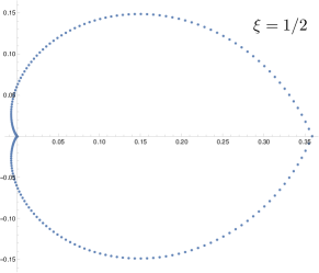
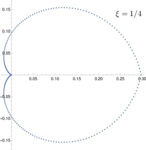
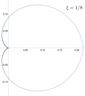
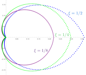
Figure 1: In the first three panels, we show the (discretized) curves $\rho_{\xi}(\varphi)$ given by eq. (14) for the values of $\xi=1/2,1/4,1/8$. The last panel shows the superposed domains.

4 The bounds and the domain of analyticity

This section is dedicated to:

Proof of Theorem 3.6.

From now on we fix $\psi\in(\theta-\pi/2,\theta+\pi/2)$ and bound $\mathfrak{K}_{\psi}^{2k}(g,\epsilon)$ (as expressed in eq. (11)) thanks to eq. (3) and the following lemma, proven in Appendix B.2:

Lemma 4.1.

Let $n$ be a positive integer, $z\in\mathbb{C}$ with $\Re z>0$, $C\in M_{n}(\mathbb{R})$ symmetric positive matrix and $F\in L^{1}(\mathbb{R}^{n},\mu_{{\lvert z\rvert^{2}C/\Re z}})$ a $\mathbb{C}$-valued function. Then:

$$\left|\int d\mu_{zC}(X)F(X)\right|=\left|\left[e^{\frac{z}{2}\langle\partial,\partial\rangle_{C}}F(X)\right]_{X=0}\right|\leq\frac{1}{\cos^{n/2}(\arg z)}\sup_{X\in\mathbb{R}^{n}}|F(X)|\,.$$ (15)

We apply this lemma with $z=\epsilon e^{-\imath\psi}$ and $C=W^{T}(u)$. Then, we bound the integration over the $u_{T}$ parameters by one. Finally, we also have to notice that $\frac{1}{\cos{(\frac{\varphi+\psi}{2})}}$ appears at the power $\sum_{i=1}^{n}d_{i}(T_{\mathfrak{c}})=k+2(n-1)$. Thus,

$$\lvert\mathfrak{K}_{\psi}^{2k}(g,\epsilon)\rvert\lesssim_{k}\frac{1}{\sqrt{\cos{(\psi-\theta)}}}\frac{1}{\cos^{k}{(\frac{\varphi+\psi}{2})}}\\ \times\sum_{n\geq k}\frac{1}{n!}{\left(\frac{\lvert g\rvert}{2\cos^{2}{(\frac{\varphi+\psi}{2})}\sqrt{\cos{(\psi-\theta)}}}\right)}^{n-1}\sum_{T_{\mathfrak{c}}\in\mathcal{T}_{n}\times C^{n}_{k}}\prod_{i=1}^{n}(d_{i}(T_{\mathfrak{c}})-1)!\;,$$

We conclude using combinatorial arguments, that are gathered in the following lemma:

Lemma 4.2.

For all $n\geq k$, the sum over $k$-ciliated (i.e. $\mathfrak{c}\in C_{k}^{n}$) trees with $n$-vertices verifies

$$\frac{1}{n!}\sum_{T_{\mathfrak{c}}\in\mathcal{T}_{n}\times C^{n}_{k}}\prod_{i=1}^{n}(d_{i}(T_{\mathfrak{c}})-1)!=\binom{2n-1}{n-k}\binom{2n+k-3}{2n-1}\times(k-2)!\;.$$

Proof.

$$\frac{1}{n!}\sum_{T_{\mathfrak{c}}\in\mathcal{T}_{n}\times C^{n}_{k}}\prod_{i=1}^{n}(d_{i}(T_{\mathfrak{c}})-1)! =\frac{1}{n!}\sum_{T\in\mathcal{T}_{n}}\prod_{i=1}^{n}(d_{i}(T)-1)!\sum_{\mathfrak{c}\in C^{n}_{k}}\prod_{i=1}^{n}\frac{(d_{i}(T)+\mathbf{1}_{i\in\mathfrak{c}}-1)!}{(d_{i}(T)-1)!}$$

$$=\frac{1}{n!}\sum_{T\in\mathcal{T}_{n}}\prod_{i=1}^{n}(d_{i}(T)-1)!\sum_{\mathfrak{c}\in C^{n}_{k}}\prod_{i\in\mathfrak{c}}d_{i}(T)\,.$$

Here, to count the number of trees, we use Cayley’s theorem that states that:

$$\sum_{T\in\mathcal{T}_{n}}\prod_{i=1}^{n}(d_{i}(T)-1)!=(n-2)!\sum^{n}_{\begin{subarray}{c}d_{1},\dotsc,d_{n}=1\\ \sum_{i}d_{i}=2(n-1)\end{subarray}}1\,,$$ (16)

which yields

$$\frac{1}{n!}\sum_{T_{\mathfrak{c}}\in\mathcal{T}_{n}\times C^{n}_{k}}\prod_{i=1}^{n}(d_{i}(T_{\mathfrak{c}})-1)!=\frac{(n-2)!}{n!}\sum^{n}_{\begin{subarray}{c}d_{1},\dotsc,d_{n}=1\\ \sum_{i}d_{i}=2(n-1)\end{subarray}}\sum_{\mathfrak{c}\in C^{n}_{k}}\prod_{i\in\mathfrak{c}}d_{i}\,.$$

The sum over the $d_{i}$’s can be computed by the following trick. Let us consider the function $f$ of $n$ variables:

$$f(x_{1},\dotsc,x_{n})=\sum_{d_{1},\dotsc,d_{n}=1}^{\infty}\prod_{i=1}^{n}x_{i}^{d_{i}}=\prod_{i=1}^{n}\frac{x_{i}}{1-x_{i}}\;.$$

Applying the following differential operator to $f$, and evaluating it at $(x,\dotsc,x)$ gives the expression of the sum as a Taylor coefficient:

$$\sum_{\begin{subarray}{c}d_{1},\dotsc,d_{n}=1\\ \sum_{i}d_{i}=2(n-1)\end{subarray}}^{\infty}\prod_{i\in\mathfrak{c}}d_{i} =[x^{2(n-1)}]\big{(}\prod_{i\in\mathfrak{c}}x_{i}\frac{\partial}{\partial x_{i}}\big{)}f(x,\dotsc,x)$$

$$=[x^{2(n-1)}]\frac{x^{n}}{(1-x)^{n+k}}=\binom{2n+k-3}{n-2}.$$

With this result at hand, and using $\sum_{\mathfrak{c}\in C^{n}_{k}}1=n!/(n-k)!$, we finally obtain that

$$\frac{1}{n!}\sum_{T_{\mathfrak{c}}\in\mathcal{T}_{n}\times C^{n}_{k}}\prod_{i=1}^{n}(d_{i}(T_{\mathfrak{c}})-1)! =\frac{(n-2)!}{n!}\times\frac{n!}{(n-k)!}\binom{2n+k-3}{n-2}=\binom{2n-1}{n-k}\binom{2n+k-3}{2n-1}\times(k-2)!\,.$$

∎

Combining this with the trigonometric identity $2\cos^{2}{(x/2)}=(1+\cos x)$, we obtain the following bound on the cumulants:

$$\lvert\mathfrak{K}_{\psi}^{2k}(g,\epsilon)\rvert\lesssim_{k}\frac{(k-2)!}{\sqrt{\cos{(\psi-\theta)}}}{\frac{1}{\cos^{k}{(\frac{\varphi+\psi}{2})}}}\\ \times\sum_{n\geq k}\binom{2n-1}{n-k}\binom{2n+k-3}{2n-1}{\left(\frac{\lvert g\rvert}{(1+\cos{(\varphi+\psi}))\sqrt{\cos{(\psi-\theta)}}}\right)}^{n-1}.$$

By Stirling’s formula, $\binom{2n-1}{n-k}\lesssim_{k}4^{n}$ and $\binom{2n+k-3}{2n-1}(k-2)!=\frac{(2n+k-3)!}{(2n-1)!}\lesssim_{k}n^{k-2}$ so that we can finally bound the cumulants by:

$$\lvert\mathfrak{K}_{\psi}^{2k}(g,\epsilon)\rvert\lesssim_{k}\frac{1}{\sqrt{\cos{(\psi-\theta)}}}{\frac{1}{\cos^{k}{(\frac{\varphi+\psi}{2})}}}\sum_{n\geq k}{\left(\frac{4\lvert g\rvert}{(1+\cos{(\varphi+\psi}))\sqrt{\cos{(\psi-\theta)}}}\right)}^{n-1}n^{k-2}\;.$$

We conclude on the analyticity of the cumulants thanks to two classical theorems: the first one states that the integral of a function that depends analytically on a paramater defines an analytic function as long as it converges; the second one states that a uniformly convergent series of analytic functions is analytic.

The cumulants are expressed as a uniformly convergent series of analytic functions both in $\Pi g$ and $\epsilon$. Since the theorems above apply in the bivariate analytic case $\mathfrak{K}_{\psi}^{2k}(g,\epsilon)$ is analytic on the domain of $\Sigma\times\mathrm{H}$ where the conditions (12) hold and analytically continues $\mathfrak{K}^{2k}(g,\epsilon)$. Taking the union of these domains for $\psi\in(\theta-\pi/2,\theta+\pi/2)$ yields an analytic continuation of $\mathfrak{K}^{2k}(g,\epsilon)$ to the subdomain $\mathfrak{C}$ of $\Sigma\times\mathrm{H}$ which concludes the proof. ∎

Remark 4.3.

For $g$ such that $\Pi g\in\mathbb{R}_{-}$, Borel summability in $\epsilon$ is lost since for $\varphi=\pm\pi$, the cardioid (12a) shrinks to zero when $\theta\rightarrow\pm\pi/2$. However, the domain of analyticity we found passes beyond the negative real axis and continues on the Riemann sheet. At the negative real axis the cumulants converge for $|\Pi g|\leq\frac{1}{6\sqrt{3}}$ which is of order 1. Of course, the cumulants are discontinuous here: the analytic continuations coming from above and from below the negative real axis do not coincide.

The discontinuity of the partition function and its logarithm are well understood as non perturbative instanton contributions: in zero dimensions and for $N=1$ this is detailed for instance in [ABS19]. On the contrary, the discontinuities of the cumulants have so far been less well studied.

Proof.

It is possible to make use of $\psi$ in order to reach the negative real axis for $g$. Indeed, assuming $\epsilon$ real positive, so that $\theta=0$, we let $z_{\psi}(\varphi)=\frac{1}{2}\cos^{2}\mathinner{\bigl{(}\frac{\varphi+\psi}{2}\bigr{)}}\sqrt{\cos\psi}\,e^{i\varphi}$ be a point on the boundary of the cardioid $\{|g|<\frac{1}{2}\cos^{2}(\frac{\varphi+\psi}{2})\sqrt{\cos\psi}\}$ The maximal value of $|z_{\psi}(\pm\pi)|$ is attained for $\psi_{0}=2\arcsin\big{(}\frac{1}{\sqrt{3}}\big{)}$ and is $\frac{1}{6\sqrt{3}}$. ∎

5 Borel summability of the cumulants in $\mathbf{1/N}$

This last section is devoted to:

Proof of Lemma 3.9.

The Borel summability of the cumulants stems from the analyticity in a Sokal disk as stated in Theorem 3.6 and an estimation of the Taylor remainder. As we aim to obtain Borel summability in $\epsilon$ uniformly in $g$, we need to show that at large $q$ the remainder of order $q$ is bounded from above by $C\,K^{q}\,\lvert\epsilon\rvert^{q}\,q!$ with $C$ and $K$ independent of $g$.

In order to compute the Taylor reminder of order $q$ we start from the expansion of $\mathfrak{K}_{\psi}^{2k}(g,\epsilon)$ in eq. (11). We fix some $\psi\in(\theta-\pi/2,\theta+\pi/2)$. Then, for all $k\geq 1$ and $(g,\epsilon)\in\mathfrak{C}$ such that $\lvert\varphi+\psi\rvert<\pi$, the cumulants read (recall the ($\star$ ‣ 3) convention):

$$\mathfrak{K}_{\psi}^{2k}(g,\epsilon)=2^{k-1}\sum_{n\geq k}\frac{1}{n!}{\left(\frac{-\Pi g}{2}\right)}^{n-1}\sum_{T_{\mathfrak{c}}\in\mathcal{T}_{n}\times C^{n}_{k}}\int du_{T}\\ \times\bigg{[}e^{t\frac{\epsilon e^{-\imath\psi}}{2}\langle\partial,\partial\rangle_{W^{T}(u)}}\prod_{i=1}^{n}\bigg{\{}(d_{i}(T_{\mathfrak{c}})-1)!\,\widetilde{R}^{d_{i}(T_{\mathfrak{c}})}(\sigma^{(i)}e^{\imath\frac{\psi}{2}},g)\bigg{\}}\bigg{]}_{\sigma^{(i)}=0,t=1}\;,$$

and the Taylor remainder of order $q$ of $\mathfrak{K}_{\psi}^{2k}(g,\epsilon)$, denoted by $R^{2k}_{q,\psi}(g,\epsilon)$ writes:

$$R^{2k}_{q,\psi}(g,\epsilon)=\int_{0}^{1}ds\frac{(1-s)^{q-1}}{(q-1)!}2^{k-1}\sum_{n\geq k}\frac{1}{n!}{\left(\frac{-\Pi g}{2}\right)}^{n-1}\sum_{T_{\mathfrak{c}}\in\mathcal{T}_{n}\times C^{n}_{k}}\int du_{T}\int d\mu_{s\epsilon e^{-\imath\psi}W^{T}(u)}(\sigma)\\ \times{\left(\frac{\epsilon e^{-\imath\psi}}{2}\right)}^{q}{\left(\langle\partial,\partial\rangle_{W^{T}(u)}\right)}^{q}\bigg{[}\prod_{i=1}^{n}\bigg{\{}(d_{i}(T_{\mathfrak{c}})-1)!\,\widetilde{R}^{d_{i}(T_{\mathfrak{c}})}(\sigma^{(i)}e^{\imath\frac{\psi}{2}},g)\bigg{\}}\bigg{]}.$$ (17)

We would like to reexpress the remainder as a sum over some graphs. Since $2q$ derivatives are going to act on each term of the sum over the ciliated trees, and since they can act on each of the $n$ vertices, to the amplitude of a ciliated tree $T_{\mathfrak{c}}$ are now going to correspond $n^{2q}$ amplitudes indexed by marks $\mathfrak{m}$ in $D^{n}_{2q}=\{1,...,n\}^{2q}$ corresponding to the ordered sequence of vertices on which the derivatives are acting (that is to say that for all $j\in\{1,...,2q\}$, the vertex $\mathfrak{m}_{j}$ is the vertex on which acted the $j$-th derivative in eq. (17)). This allows us to index the sum (17) by decorated trees, for which we adopt the next convention:

$$\text{triples $(T,\mathfrak{c},\mathfrak{m})$ made of a tree $T\in\mathcal{T}_{n}$, \emph{cilia} $\mathfrak{c}\in C^{n}_{k}$ and \emph{marks} $\mathfrak{m}\in D^{n}_{2q}$ are denoted by $T_{\mathfrak{c},\mathfrak{m}}$}. \star\! \star$$ ( )

For all $i\in\{1,...,n\}$, we also denote by $d_{i}(T_{\mathfrak{c},\mathfrak{m}})=m(i)+d_{i}(T_{\mathfrak{c}})=m(i)+c(i)+d_{i}(T)$ the coordination degree of the vertex $i$ in the decorated tree $T_{\mathfrak{c},\mathfrak{m}}$, with $m(i)=\lvert\{j\in\{1,...,2q\}\mid\mathfrak{m}_{j}=i\}\rvert$ the number of marks of $i$ and $c(i)=\textbf{1}_{i\in\mathfrak{c}}$ the number of cilia of $i$, which is 0 or 1. With this notation, the rest term rewrites (recall that with the convention ($\star\!$ $\star$ ‣ 5), $T$ is the tree $T_{\mathfrak{c},\mathfrak{m}}$ without cilia and marks):

$$R^{2k}_{q,\psi}(g,\epsilon)=2^{k}(-\epsilon)^{q}\int_{0}^{1}ds\frac{(1-s)^{q-1}}{(q-1)!}\sum_{n\geq k}\frac{1}{2^{n}n!}{\left(-\Pi g\right)}^{n-1+q}\sum_{T_{\mathfrak{c},\mathfrak{m}}\in\mathcal{T}_{n}\times C^{n}_{k}\times D^{n}_{2q}}\\ \times\int du_{T}\int d\mu_{s\epsilon e^{-\imath\psi}W^{T}(u)}(\sigma)\prod_{\ell=1}^{q}W^{T}_{\mathfrak{m}_{2\ell-1}\mathfrak{m}_{2\ell}}(u)\prod_{i=1}^{n}\big{\{}(d_{i}(T_{\mathfrak{c},\mathfrak{m}})-1)!\,\widetilde{R}^{d_{i}(T_{\mathfrak{c},\mathfrak{m}})}(\sigma^{(i)}e^{\imath\frac{\psi}{2}},g)\big{\}}.$$

The remainder can now be bounded using the same arguments as in Section 4, but taking into account the combinatorics of the new $2q$ derivatives that can act on a ciliated tree $T_{\mathfrak{c}}$. We have the following lemma:

Lemma 5.1.

For all $n\geq k$, $q\geq 0$, the sum over $k$-ciliated (i.e. $\mathfrak{c}\in C_{k}^{n}$) and $2q$-marked (i.e. $\mathfrak{m}\in D_{2q}^{n}$) trees with $n$-vertices verifies

$$\frac{1}{n!}\sum_{T_{\mathfrak{c},\mathfrak{m}}\in\mathcal{T}_{n}\times C^{n}_{k}\times D^{n}_{2q}}\prod_{i=1}^{n}(d_{i}(T_{\mathfrak{c},\mathfrak{m}})-1)!=\binom{2n-1}{n-k}\binom{2n+2q+k-3}{2n-1}\times(2q+k-2)!\;.$$ (18)

In particular, for $q=0$ we recover Lemma 4.2.

Proof of Lemma 3.9.

Injecting Cayley’s formula (16) in eq. (18) yields

$$\frac{1}{n!}\sum_{T_{\mathfrak{c},\mathfrak{m}}\in\mathcal{T}_{n}\times C^{n}_{k}\times D^{n}_{2q}}\prod_{i=1}^{n}(d_{i}(T_{\mathfrak{c},\mathfrak{m}})-1)! =\frac{(n-2)!}{n!}\sum^{n}_{\begin{subarray}{c}d_{1},...,d_{n}=1\\ \sum_{i}d_{i}=2n-2\end{subarray}}\sum_{\mathfrak{c}\in C^{n}_{k}}\sum_{\mathfrak{m}\in D^{n}_{2q}}\prod_{i=1}^{n}\frac{(d_{i}+c(i)+m(i)-1)!}{(d_{i}-1)!}$$

$$=\frac{(n-2)!}{n!}\sum^{n}_{\begin{subarray}{c}d_{1},...,d_{n}=1\\ \sum_{i}d_{i}=2n-2\end{subarray}}\sum_{\mathfrak{c}\in C^{n}_{k}}\prod_{i\in\mathfrak{c}}d_{i}\sum_{\mathfrak{m}\in D^{n}_{2q}}\prod_{i=1}^{n}\frac{(d_{i}+c(i)+m(i)-1)!}{(d_{i}+c(i)-1)!}\;.$$

Then, using

$$\sum_{\mathfrak{m}\in D^{n}_{2q}}\prod_{i=1}^{n}\frac{(d_{i}+c(i)+m(i)-1)!}{(d_{i}+c(i)-1)!} =\sum_{\begin{subarray}{c}m(1),...,m(n)\\ \sum_{i}m(i)=2q\end{subarray}}\frac{(2q)!}{\prod_{i=1}^{n}m(i)!}\prod_{i=1}^{n}\frac{(d_{i}+c(i)+m(i)-1)!}{(d_{i}+c(i)-1)!}$$

$$=(2q)!\sum_{\begin{subarray}{c}m(1),...,m(n)\\ \sum_{i}m(i)=2q\end{subarray}}\prod_{i=1}^{n}\binom{d_{i}+c(i)+m(i)-1}{m(i)}$$

$$=(2q)![x^{2q}]\prod_{i=1}^{n}\frac{1}{(1-x)^{d_{i}+c(i)}}=(2q)![x^{2q}]\frac{1}{(1-x)^{2n-2+k}}$$

$$=(2q)!\binom{2n-2+k+2q-1}{2q}=\frac{(2n+2q+k-3)!}{(2n+k-3)!}\,,$$

$\sum_{\mathfrak{c}\in C^{n}_{k}}1=n!/(n-k)!$ and $\sum^{n}_{\begin{subarray}{c}d_{1},...,d_{n}=1\\ \sum_{i}d_{i}=2n-2\end{subarray}}\prod_{i\in\mathfrak{c}}d_{i}=\binom{2n+k-3}{n+k-1}$, we get:

$$\frac{1}{n!}\sum_{T_{\mathfrak{c},\mathfrak{m}}\in\mathcal{T}_{n}\times C^{n}_{k}\times D^{n}_{2q}}\prod_{i=1}^{n}(d_{i}(T_{\mathfrak{c},\mathfrak{m}})-1)! =\frac{(n-2)!}{n!}\times\frac{n!}{(n-k)!}\binom{2n+k-3}{n+k-1}\frac{(2n+2q+k-3)!}{(2n+k-3)!}$$

$$=\binom{2n-1}{n-k}\binom{2n+2q+k-3}{2n-1}\times(2q+k-2)!\;.$$

∎

Thanks to this lemma, we can now find an upper bound on the rest term. All the entries of the $W^{T}(u)$ matrices are bounded by one, and eq. (13a) implies that $\lvert g\rvert^{q}$ is smaller than $1/2^{q}$. We also use Lemma B.4 to bound the integration over $\sigma$, and we trivially bound all the integrals over $s$ and the $u_{T}$’s by one leading to:

$$\lvert R^{2k}_{q,\psi}(g,\epsilon)\rvert\lesssim_{k}\,\left(\frac{|\epsilon\rvert}{2}\right)^{q}\frac{(2q+k-2)!}{(q-1)!}\sum_{n\geq k}\binom{2n-1}{n-k}\binom{2n+2q+k-3}{2n-1}{\left(\frac{\lvert g\rvert}{2}\right)}^{n-1}\\ \times{\left(\frac{1}{\sqrt{\cos{(\psi-\theta)}}}\right)}^{\!n}{\left(\frac{2}{1+\cos{(\varphi+\psi)}}\right)}^{\!n+q+\frac{k}{2}-1}.$$

Now, let us choose some small $\alpha>0$, and take $(g,\epsilon)\in\mathfrak{C}_{\alpha}$, that is to say such that the inequalities (13) are satisfied. Note that in this domain, $g$ and $\epsilon$ satisfy tighter bounds, which are gathered in the following lemma:

Lemma 5.2.

For small $\alpha>0$, and for all $(g,\epsilon)\in\mathfrak{C}$ such that (13) hold, we have:

$$\alpha^{2} \leq\frac{1+\cos{(\varphi+\psi)}}{2}\leq 1$$ (19a)

$$\sqrt{\alpha} \leq\sqrt{\cos{(\psi-\theta)}}\leq 1$$ (19b)

$$\frac{\alpha}{2} \leq 1-\sqrt{\gamma}\leq 1\qquad\qquad\text{with }\gamma=\frac{4\lvert g\rvert}{{(1+\cos{(\varphi+\psi)})\sqrt{\cos{(\psi-\theta)}}}}\;.$$ (19c)

Proof..

Since $0\leq\lvert\varphi+\psi\rvert\leq\pi(1-\alpha)$, $\cos^{2}{\frac{\pi(1-\alpha)}{2}}\leq\cos^{2}{\frac{\lvert\varphi+\psi\rvert}{2}}\leq 1$, and $\cos^{2}{\frac{\pi(1-\alpha)}{2}}=\sin^{2}{\frac{\pi\alpha}{2}}\geq\alpha^{2}$ for small $\alpha>0$. Similarly, since $0\leq\lvert\psi-\theta\rvert\leq\frac{\pi}{2}(1-\alpha)$, $\cos{(\frac{\pi}{2}(1-\alpha))}\leq\cos{\lvert\psi-\theta\rvert}\leq 1$ so that $\sqrt{\cos{(\frac{\pi}{2}(1-\alpha))}}\leq\sqrt{\cos{\lvert\psi-\theta\rvert}}\leq 1$ and $\sqrt{\cos{(\frac{\pi}{2}(1-\alpha))}}=\sqrt{\sin{(\frac{\pi\alpha}{2}})}\geq\sqrt{\alpha}$ for small $\alpha>0$. Finally, since $0\leq\gamma\leq 1-\alpha$, $0\leq\sqrt{\gamma}\leq\sqrt{1-\alpha}$ and $\sqrt{1-\alpha}\leq 1-\frac{\alpha}{2}$ for small $\alpha>0$ so that $\frac{\alpha}{2}\leq 1-\sqrt{\gamma}\leq 1$. ∎

Combining this with the bounds in eqs. (3) and (15), and using $(2q+k-2)!/(q-1)!\lesssim_{k}4^{q}q!$ and $\binom{2n-1}{n-k}\leq 4^{n}$ by Stirling’s formula, we obtain the following upper bound on the rest term:

$$\lvert R^{2k}_{q,\psi}(g,\epsilon)\rvert\lesssim_{k} {}{|\epsilon\rvert}^{q}2^{q}q!\sum_{n\geq k}\binom{2n+2q+k-3}{2n-1}{\left(\frac{4\lvert g\rvert}{(1+\cos{(\varphi+\psi)})\sqrt{\cos{(\psi-\theta)}}}\right)}^{n-1}$$

$$\times{\left(\frac{2}{1+\cos{(\varphi+\psi)}}\right)}^{q+\frac{k}{2}}{\left(\frac{1}{\sqrt{\cos{(\psi-\theta)}}}\right)}$$

$$\lesssim_{k} {}(\alpha^{2})^{-q-\frac{k}{2}}(\sqrt{\alpha})^{-1}{|\epsilon\rvert}^{q}2^{q}q!\sum_{n\geq k}\binom{2n+2q+k-3}{2n-1}{\gamma}^{n-1}.$$

Recall that $\gamma\in[0,1-\alpha\mathopen{]}$ in $\mathfrak{C}_{\alpha}$. Let us denote $f(\gamma)=\sum_{n\geq k}\binom{2n+2q+k-3}{2n-1}{\gamma}^{n-1}$ so that:

$$\lvert R^{2k}_{q}(g,\epsilon)\rvert\lesssim_{k}\alpha^{-1/2-k-2q}{|\epsilon\rvert}^{q}2^{q}q!f(\gamma).$$

In order to conclude, it suffices to prove that $f(\gamma)$ is exponentially bounded in $q$ for all $\gamma\in[0,1-\alpha\mathopen{]}$. This is stated in the following lemma:

Lemma 5.3.

At large $q$, for all $\gamma\in[0,1-\alpha\mathopen{]}$, we have that

$$f(\gamma)\leq\frac{4q}{{(1-\sqrt{\gamma})}^{2q+k}}.$$

Proof..

We note that $\binom{2n+2q+k-3}{2n-1}=\frac{2q+k-1}{2n-1}\binom{2n+2q+k-3}{2n-2}$ and that for any $k$ and $n$, for $q$ large enough $\frac{2q+k-1}{2n-1}\leq 4q$ so that $\binom{2n+2q+k-3}{2n-1}\leq 4q\binom{2n+2q+k-3}{2n-2}$. This implies that for all $k\geq 1$:

$$f(\gamma) =\sum_{n\geq k}\binom{2n+2q+k-3}{2n-1}{\gamma}^{n-1}\leq 4q\sum_{n\geq k}\binom{2n+2q+k-3}{2n-2}{\gamma}^{n-1}$$

$$\leq 4q\sum_{n\geq k}\binom{2n+2q+k-3}{2n-2}{(\sqrt{\gamma})}^{2n-2}\leq 4q\sum_{n\geq 2k-2}\binom{n+2q+k-1}{n}{(\sqrt{\gamma})}^{n}$$

$$\leq 4q\sum_{n\geq 0}\binom{n+2q+k-1}{n}{(\sqrt{\gamma})}^{n}\;.$$

In the second line we bound the even part of the series by the total series, using the positivity of the odd part. Observing that $\sum_{n\geq 0}\binom{n+2q+k-1}{n}\sqrt{\gamma}^{n}=\frac{1}{{(1-\sqrt{\gamma})}^{2q+k}}$ we are done. ∎

Combining this lemma with eq. (19c), we can bound $f$ uniformly as $f(\gamma)\lesssim_{k}\frac{4q}{\alpha^{2q+k}}$ for all $\gamma\in[0,1-\alpha\mathopen{]}$ and denoting $C_{\alpha}=\alpha^{-2k-1/2}$ and $K_{\alpha}=6\alpha^{-4}$ at $q$ large enough, for all $k\geq 1$:

$$\lvert R^{2k}_{q,\psi}(g,\epsilon)\rvert\lesssim_{k}C_{\alpha}K_{\alpha}^{q}{\lvert\epsilon\rvert}^{q}q!\;,$$

with $C_{\alpha}$ and $K_{\alpha}$ independent of $g$ for $g\in\mathfrak{C}_{\alpha}$, which concludes the proof of lemma (3.9).∎

Remark 5.4.

Note that, as $K_{\alpha}\sim O(1)\alpha^{-4}$ and $C_{\alpha}\sim{\alpha^{-2k-1/2}}$ our bounds deteriorate for $\alpha\to 0$ that is when we take a subdomain closer and closer to the full $\mathfrak{C}$.

Conclusion

The Loop Vertex Expansion made possible to extract the logarithm of the partition function, obtain the maximal analyticity domain (Thm. 3.6), and the domain of $1/N$-Borel summability (Thm. 3.8) of the cumulants of the quartic $\mathrm{O}(N)$-vector model.

The next step would be to adapt our analysis to the more involved case of a (Euclidean) quantum field theory. The fist case of interest is the two dimensional quartic $\mathrm{O}(N)$-vector model, whose renormalisation is limited to the Wick ordering. Two dimensional quantum field theory was studied with a modification of the LVE known as the Multiscale LVE (MLVE) in [RW15], where the Borel summability of free energy in the coupling constant is established. This study should be generalized to an $\mathrm{O}(N)$-vector model. However, the adaptation of the (M)LVE beyond dimension two seems out of reach.

Appendix A The Nevalinna-Sokal theorem

A formal power series $A(z)=\sum_{k=0}^{\infty}a_{k}z^{k}$ such that $B(t)=\sum_{k=0}^{\infty}a_{k}/k!t^{k}$ is absolutely convergent in some disk centered at zero an admits an analytic continuation along the real axis such that $|B(t)|<Ke^{-t/R}$ for some $K,R\in\mathbb{R}_{+}$ is called a Borel summable series. The function $\sum_{k=0}^{\infty}a_{k}/k!t^{k}$ is called the Borel transform of $A(z)$ and the Borel sum of $A(z)$ is the Laplace transform of its Borel transform:

$$f(z)=\frac{1}{z}\int_{0}^{\infty}dt\;e^{-t/z}B(t)\;.$$

The Borel sum of a series, if it exists, is unique.

A function $f\mathrel{\mathop{\mathchar 58\relax}}\mathbb{C}\rightarrow\mathbb{C}$ which is analytic in a disk tangent to the imaginary axis in $0$ and has an asymptotic series in $0$ (which can have zero radius of convergence) such that the Taylor rest term of order $q$ in $0$ of $f$ grows no faster than $q!$ is called a Borel summable function [Sok79].

These two notions are intimately related: the Borel sums of Borel summable series are Borel summable functions (this is straightforward to prove). The asymptotic series of Borel summable functions are Borel summable series [Sok79]. We present here a slightly modified version [Riv07] of the (optimal) Nevanlinna-Sokal theorem on Borel summability which introduces the notion of uniform Borel summability with respect to some parameter.

Theorem A.1 (Nevanlinna-Sokal).

Let $f$ be a function $f\mathrel{\mathop{\mathchar 58\relax}}\mathbb{C}^{2}\rightarrow\mathbb{C}$, $(z,w)\mapsto f(z,w)$ and let $(f_{k}(w))_{k\geq 0}$ be the coefficients of the asymptotic series of $f$ in $z=0$, at fixed $w\in\mathbb{C}$. If $f$ is analytic in its first variable $z$ in a domain ${\rm Disk}_{R}=\{z\in\mathbb{C}\mid\Re{(1/z)}>1/R\}$ with $R>0$ independent of $w$ and there is a domain $\cal D\subset\mathbb{C}$ such that for all $(z,w)\in{\rm Disk}_{R}\times{\cal D}$, there exist some constants $C,K>0$ independent of $w$ for which the following bound on the rest term of $f$ holds for $q$ large enough:

$$\left|f(z,w)-\sum_{k=0}^{q}f_{k}(w)z^{k}\right|\leq CK^{q}\lvert z\rvert^{q}q!,$$

then $f$ is called a Borel summable function in $z$ uniformly in $w$ in ${\rm Disk}_{R}\times{\cal D}$.

Under these conditions, for all $w\in\cal D$, the Borel transform in $z$ of the asymptotic series of $f$,

$$\mathcal{B}\mathrel{\mathop{\mathchar 58\relax}}(t,w)\mapsto\sum_{k=0}^{+\infty}\frac{f_{k}(w)}{k!}t^{k},$$

is analytic in a disk of radius $K^{-1}$ in $t$ and can be analytically continued to the strip $\{t\in\mathbb{C}\mid\lvert\Im t\rvert<K^{-1}\}$ and in this strip obeys the exponential bound $|\mathcal{B}(t)|<e^{t/R}$. Moreover, for all $(z,w)\in{\rm Disk}_{R}\times{\cal D}$ we can reconstruct the function $f(z,w)$ by:

$$f(z,w)=\frac{1}{z}\int_{\mathbb{R}_{+}}dt\;e^{-t/z}\mathcal{B}(t,w).$$

Remark A.2.

For $R>0$, the domain $\{z\in\mathbb{C}\mid\Re{(1/z)}>1/R\}$ is a disk of diameter $R$ tangent to the imaginary axis at the origin. We call Sokal disk of diameter $R$ such a disk, see Figure 2.

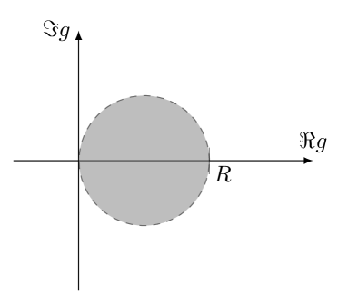
Figure 2: A Sokal disk ${\rm Disk}_{R}=\{g\in\mathbb{C}\mid\Re(1/g)>1/R\}$

Appendix B Finite dimensional Gaussian measures

B.1 Gaussian expectations

Let $n$ a strictly positive integer. We are interested in the centered Gaussian distributions on $\mathbb{R}^{n}$, that is to say the centered probability distributions on $\mathbb{R}^{n}$ such that their cumulants of order higher than or equal to three are zero.

Case $\mathbf{n=1}$. Let us first consider the one dimensional case. In this case, for $\sigma>0$, the Normal distribution of variance $\sigma^{2}$, $\mathcal{N}(0,\sigma^{2})$ is Gaussian and its density with respect to the Lebesgue measure on $\mathbb{R}$ is $(\sqrt{2\pi}\sigma)^{-1}e^{-\frac{x^{2}}{2\sigma^{2}}}$. But this is not the only Gaussian distribution on $\mathbb{R}$: the Dirac distribution $\delta$ whose expectation $\mathbb{E}_{0}$ is defined by $\mathbb{E}_{0}[F(x)]=F(0)$ for all functions $F\mathrel{\mathop{\mathchar 58\relax}}\mathbb{R}\rightarrow\mathbb{C}$ is also Gaussian with variance 0. There is no other Gaussian distributions on $\mathbb{R}$, so that the Gaussian distributions on $\mathbb{R}$ are determined by their variances and share the following property.

Definition B.1 (Gaussian distributions in dimension one).

For all $\varepsilon\in\mathbb{R}_{+}$, there exists a unique centered Gaussian distribution of variance $\varepsilon$. Let us denote it $\mu_{\varepsilon}$, and $\mathbb{E}_{\varepsilon}$ the expectation with respect to $\mu_{\varepsilon}$. For $F\mathrel{\mathop{\mathchar 58\relax}}\mathbb{R}\rightarrow\mathbb{C}\in L^{1}(\mathbb{R},\mu_{\varepsilon})$, $\mathbb{E}_{\varepsilon}$ is defined by the following identity:

$$\mathbb{E}_{\varepsilon}[F(x)]=[e^{\frac{\varepsilon}{2}\partial_{x}^{2}}F(x)]_{x=0}\;.$$

Furthermore, if $\varepsilon\neq 0$, $\mu_{\varepsilon}=\mathcal{N}(0,\varepsilon)$ and $\mu_{\varepsilon}=\delta$ otherwise.

The previous definition immediately implies that for all $F\mathrel{\mathop{\mathchar 58\relax}}\mathbb{R}\rightarrow\mathbb{C}$, $\mathbb{E}_{\varepsilon}[F(x)]\xrightarrow[\varepsilon\rightarrow 0]{}\mathbb{E}_{0}[F(x)]$, which means that $\mathcal{N}(0,\varepsilon)\xrightarrow[\varepsilon\rightarrow 0]{\text{in law}}\delta$.
Case $\mathbf{n\geq 2}$. The Gaussian distribution on $\mathbb{R}^{n}$ is a straightforward generalization of that on $\mathbb{R}$, as stated in the following definition:

Definition B.2 (Gaussian distributions in dimension $n$).

Let $C$ in $M_{n}(\mathbb{R})$ a symmetric positive matrix not necessarily invertible. There exists a unique centered Gaussian distribution of covariance $C$. Let us denote it $\mu_{C}$, and $\mathbb{E}_{C}$ the expectation with respect to $\mu_{C}$. For $F\mathrel{\mathop{\mathchar 58\relax}}\mathbb{R}^{n}\rightarrow\mathbb{C}\in L^{1}(\mathbb{R}^{n},\mu_{C})$, $\mathbb{E}_{C}$ is defined by the following identity:

$$\mathbb{E}_{C}[F(X)]=[e^{\frac{1}{2}\langle\partial,\partial\rangle_{C}}F(X)]_{X=0}\;.$$

Furthermore, if $C$ is in $GL_{n}(\mathbb{R})$, $\mu_{C}=\mathcal{N}(0,C)$ where $\mathcal{N}(0,C)$ is the Normal distribution of covariance $C$ that has density $\frac{1}{\sqrt{(2\pi)^{n}\det{C}}}e^{-\frac{1}{2}\langle X,X\rangle_{C^{-1}}}$ with respect to the Lebesgue measure on $\mathbb{R}^{n}$. If $C$ is not invertible, then $C_{\varepsilon}=C+\varepsilon P$, with $P$ the projector on the kernel of $C$ is invertible and:

$$\mathcal{N}(0,C_{\varepsilon})\xrightarrow[\varepsilon\rightarrow 0]{\text{in law}}\mu_{C}\;,$$

which implies that:

$$\mathbb{E}_{C}[F(X)]=\lim_{\varepsilon\rightarrow 0}\mathbb{E}_{\mathcal{N}(0,C_{\varepsilon})}[F(X)]=\lim_{\varepsilon\rightarrow 0}\int_{\mathbb{R}^{n}}\frac{1}{\sqrt{(2\pi)^{n}\det{C_{\varepsilon}}}}e^{-\frac{1}{2}\langle X,X\rangle_{C_{\varepsilon}^{-1}}}F(X)d^{n}X\;.$$

Once again, there are two ways of thinking of $\mu_{C}$ if $C$ is not invertible: either we see it as a differential operator or as the limit in law of a sequence of Normal distributions. Both are useful: the former makes the interpolation between different covariances more transparent, while the latter makes bounding the expectations easier.

B.2 Complex Gaussian integration

Definition B.3 (Complex Gaussian expectation).

Let $n$ be a positive integer, $z=\lvert z\rvert e^{\imath\alpha}\in\{\Re z>0\}$, $C\in M_{n}(\mathbb{R})$ symmetric positive semi-definite, and $F\in L^{1}(\mathbb{R}^{n},\mu_{{\lvert z\rvert^{2}C/\Re z}})$ a $\mathbb{C}$-valued function. We call complex Gaussian integration of covariance $zC$ the quantity denoted $\mathbb{E}_{zC}$ and defined by:

$$\mathbb{E}_{zC}[F(X)]=[e^{\frac{z}{2}\langle\partial,\partial\rangle_{C}}F(X)]_{X=0}=\lim_{\varepsilon\rightarrow 0}\mathbb{E}_{\frac{\lvert z\rvert^{2}}{\Re z}C_{\varepsilon}}[\frac{1}{\sqrt{(\cos\alpha\;e^{\imath\alpha})^{n}}}e^{\frac{\imath\Im z}{2\lvert z\rvert^{2}}\langle X,X\rangle_{C_{\varepsilon}^{-1}}}F(X)]$$

with $C_{\varepsilon}$ a sequence such that $\mathcal{N}(0,C_{\varepsilon})\rightarrow\mu_{C}$ (if $C$ is invertible, take $C_{\varepsilon}=C$ constant).

Lemma B.4 (Complex Gaussian bound).

With the same notations, if $z=|z|e^{\imath\alpha}$ with $\alpha\in(-\frac{\pi}{2},\frac{\pi}{2})$, we have that:

$$\left|\mathbb{E}_{zC}[F(X)]\right|\leq\frac{1}{\cos^{n/2}\alpha}\;\sup_{X\in\mathbb{R}^{n}}|F(X)|\;.$$

Proof.

Since for a convergent sequence the modulus and the limit commute,

$$|\mathbb{E}_{zC}[F(X)]| =|\lim_{\varepsilon\rightarrow 0}\mathbb{E}_{\frac{\lvert z\rvert^{2}}{\Re z}C_{\varepsilon}}[\frac{1}{\sqrt{(\cos\alpha e^{\imath\alpha})^{n}}}e^{\frac{\imath\Im z}{2\lvert z\rvert^{2}}\langle X,X\rangle_{C_{\varepsilon}^{-1}}}F(X)]|$$

$$=\lim_{\varepsilon\rightarrow 0}|\mathbb{E}_{\frac{\lvert z\rvert^{2}}{\Re z}C_{\varepsilon}}[\frac{1}{\sqrt{(\cos\alpha e^{\imath\alpha})^{n}}}e^{\frac{\imath\Im z}{2\lvert z\rvert^{2}}\langle X,X\rangle_{C_{\varepsilon}^{-1}}}F(X)]|$$

$$\leq\sup_{X\in\mathbb{R}^{n}}\big{|}\frac{1}{\sqrt{(\cos\alpha e^{\imath\alpha})^{n}}}e^{\frac{\imath\Im z}{2\lvert z\rvert^{2}}\langle X,X\rangle_{C_{\varepsilon}^{-1}}}F(X)\big{|}=\frac{1}{\cos^{n/2}\alpha}\;\sup_{X\in\mathbb{R}^{n}}|F(X)|\;.$$

∎

B.3 The copies trick

Lemma B.5 (The copies trick).

Let $n$ be a positive integer, $z\in\{\Re z>0\}$ and $F\in L^{n}(\mathbb{R},\mu_{\lvert z\rvert^{2}/\Re z})$ a $\mathbb{C}$-valued function. Then $F^{\otimes n}\mathrel{\mathop{\mathchar 58\relax}}\mathbb{R}^{n}\to\mathbb{C}$, $(X_{i})_{1\leq i\leq n}\mapsto\prod_{1=n}^{n}F(X_{i})$ is in $L^{1}(\mathbb{R}^{n},\mu_{{\lvert z\rvert^{2}\mathbbm{1}_{n}/\Re z}})$ and furthermore we have:

$$\mathbb{E}_{z}[F^{n}(x)]=\mathbb{E}_{z\mathbbm{1}_{n}}[F^{\otimes n}(X)]$$

Proof.

For simplicity we take $z=1$. We denote by $u$ the vector of $\mathbb{R}^{n}$ with all entries $1/\sqrt{n}$, such that $\mathbbm{1}_{n}=nu\otimes u$. Let $v_{2},...,v_{n}\in\mathbb{R}^{n}$ such that $(u,v_{2},...,v_{n})$ is an orthonormal basis of $\mathbb{R}^{n}$. We aim to understand the action of $\mu_{\mathbbm{1}_{n}}$ on a test function $G\mathrel{\mathop{\mathchar 58\relax}}\mathbb{R}^{n}\rightarrow\mathbb{C}$. For $\varepsilon>0$, let us define $C_{\varepsilon}$ by $C_{\varepsilon}=\mathbbm{1}_{n}+\varepsilon\sum_{i=2}^{n}v_{i}\otimes v_{i}$ so that $C_{\varepsilon}\rightarrow\mathbbm{1}_{n}$ as $\varepsilon\rightarrow 0$. Then,

$$\mathbb{E}_{\mathbbm{1}_{n}}[G(X)] =\lim_{\varepsilon\rightarrow 0}\int_{\mathbb{R}^{n}}\frac{1}{\sqrt{(2\pi)^{n}\det{C_{\varepsilon}}}}e^{-\frac{1}{2}\langle X,X\rangle_{C_{\varepsilon}^{-1}}}G(X)d^{n}X$$

$$=\lim_{\varepsilon\rightarrow 0}\int_{\mathbb{R}^{n}}\frac{1}{\sqrt{(2\pi)^{n}n\varepsilon^{n-1}}}e^{-\frac{1}{2}(n^{-1}y_{1}^{2}+\varepsilon^{-1}\sum_{i=2}^{n}y_{i}^{2})}G(y_{1}u+\sum_{i=2}^{n}y_{i}v_{i})\,dy_{1}\prod_{i=1}^{n}dy_{i}$$

$$=\lim_{\varepsilon\rightarrow 0}\int_{\mathbb{R}^{n}}\frac{1}{\sqrt{(2\pi)^{n}\varepsilon^{n-1}}}e^{-\frac{1}{2}(y_{1}^{2}+\varepsilon^{-1}\sum_{i=2}^{n}y_{i}^{2})}G(y_{1}\sqrt{n}u+\sum_{i=2}^{n}y_{i}v_{i})\,dy_{1}\prod_{i=1}^{n}dy_{i}$$

$$=\lim_{\varepsilon\rightarrow 0}\mathbb{E}_{1\otimes\varepsilon^{\otimes(n-1)}}[G(y_{1}\sqrt{n}u+\sum_{i=2}^{n}y_{i}v_{i})]$$

$$=\mathbb{E}_{1\otimes 0^{\otimes(n-1)}}[G(y_{1}\sqrt{n}u+\sum_{i=2}^{n}y_{i}v_{i})]$$

$$=\mathbb{E}_{1}[G(y_{1},...,y_{1})]$$

To go from the first to the second line, we perform a change of variable from $X$ to $Y=y_{1}u+\sum_{i=2}^{n}y_{i}v_{i}$ whose Jacobian determinant is 1, and to go from the second line to the third line, we perform the change of variable $y_{1}$ becomes $\sqrt{n}y_{1}$. Line four is a simple rewriting of line three with $y_{1}\sim\mu_{1}$ and $y_{i}\sim\mu_{\varepsilon}$ for all $2\leq i\leq n$, and going from line four to line five uses the convergence in law of the Normal distribution to the Dirac distribution, while line six is simply the expectation of the Dirac measure.

Applying the previous equality to $G=F^{\otimes n}$ and substituting $\mathbbm{1}_{n}$ with $z\mathbbm{1}_{n}$ concludes the proof. ∎

References

- [ABS19] Inês Aniceto, Gökçe Başar and Ricardo Schiappa “A primer on resurgent transseries and their asymptotics” In Phys. Rept. 809, 2019, pp. 1–135 DOI: 10.1016/j.physrep.2019.02.003
- [AR95] Abdelmalek Abdesselam and Vincent Rivasseau “Trees, forests and jungles: a botanical garden for cluster expansions” In Constructive Physics 446, Lectures Notes in Physics New York: Springer-Verlag, 1995
- [BK87] David C. Brydges and T. Kennedy “Mayer expansions and the Hamilton-Jacobi equation” In J. Stat. Phys. 48.1, 1987, pp. 19–49 DOI: 10.1007/BF01010398
- [BR82] Claude Billionnet and Pierre Renouard “Analytic interpolation and Borel summability of the models” In Commun. Math. Phys. 84, 1982, pp. 257–295 DOI: 10.1007/BF01208572
- [DR16] Thibault Delepouve and Vincent Rivasseau “Constructive Tensor Field Theory: The Model” In Commun. Math. Phys. 345.2, 2016, pp. 477–506 DOI: 10.1007/s00220-016-2680-1
- [EMS74] Jean-Pierre Eckmann, Jacques Magnen and R. Sénéor “Decay properties and borel summability for the Schwinger functions in theories” In Commun. Math. Phys. 39.4, 1974, pp. 251–271
- [FMR82] Jürg Fröhlich, A. Mardin and Vincent Rivasseau “Borel summability of the expansion for the -vector [ non-linear ] models” In Commun. Math. Phys. 86, 1982, pp. 87–110 DOI: 10.1007/BF01205663
- [GK15] Răzvan Gurău and Thomas Krajewski “Analyticity results for the cumulants in a random matrix model” In Ann. Inst. Henri Poincaré Comb. Phys. Interact. 2.2, 2015, pp. 169–228 DOI: 10.4171/AIHPD/17
- [Gur13] Răzvan Gurău “The Expansion of Tensor Models Beyond Perturbation Theory” In Commun. Math. Phys. 330.3, 2013, pp. 973–1019 arXiv:1304.2666 [math-ph]
- [Hub59] J. Hubbard “Calculation of Partition Functions” In Phys. Rev. Lett. 3 American Physical Society, 1959, pp. 77–78 DOI: 10.1103/PhysRevLett.3.77
- [Kup80] Antti J. Kupiainen “ expansion for a Quantum Field Model” In Commun. Math. Phys. 74.3, 1980, pp. 199–222 DOI: 10.1007/BF01952886
- [Kup80a] Antti J. Kupiainen “On the Expansion” In Commun. Math. Phys. 73.3, 1980, pp. 273–294 DOI: 10.1007/BF01197703
- [MR07] Jacques Magnen and Vincent Rivasseau “Constructive Field Theory without Tears” In Ann. H. Poincaré 9, 2007, pp. 403–424 arXiv:0706.2457 [math-ph]
- [Riv07] Vincent Rivasseau “Constructive Matrix Theory” In J. High Energ. Phys. 09.008, 2007 arXiv:0706.1224 [hep-th]
- [Riv09] Vincent Rivasseau “Constructive Field Theory in Zero Dimension” In Adv. Math. Phys., 2009 DOI: 10.1155/2009/180159
- [RVT18] Vincent Rivasseau and Fabien Vignes-Tourneret “Constructive Tensor Field Theory: The Model” In Commun. Math. Phys. 366.2, 2018, pp. 567–646 DOI: 10.1007/s00220-019-03369-9
- [RW15] Vincent Rivasseau and Zhituo Wang “Corrected Loop Vertex Expansion for Theory” In Journal of Mathematical Physics 56.6, 2015, pp. 062301 DOI: 10.1063/1.4922116
- [Sok79] Alan D. Sokal “An improvement of Watson’s theorem on Borel summability” In Journ. Math. Phys. 21.2, 1979, pp. 261–263
- [Str57] R. L. Stratonovich “On a Method of Calculating Quantum Distribution Functions” In Soviet Physics Doklady 2, 1957, pp. 416