A cost-based multi-layer network approach for the discovery of patient phenotypes

Abstract

Clinical records frequently include assessments of the characteristics of patients, which may include the completion of various questionnaires. These questionnaires provide a variety of perspectives on a patient’s current state of well-being. Not only is it critical to capture the heterogeneity given by these perspectives, but there is also a growing demand for developing cost-effective technologies for clinical phenotyping. Filling out many questionnaires may be a strain for the patients and therefore costly. In this work, we propose COBALT - a cost-based layer selector model for detecting phenotypes using a community detection approach. Our goal is to minimize the number of features used to build these phenotypes while preserving its quality. We test our model using questionnaire data from chronic tinnitus patients and represent the data in a multi-layer network structure. The model is then evaluated by predicting post-treatment data using baseline features (age, gender, and pre-treatment data) as well as the identified phenotypes as a feature. For some post-treatment variables, predictors using phenotypes from COBALT as features outperformed those using phenotypes detected by traditional clustering methods. Moreover, using phenotype data to predict post-treatment data proved beneficial in comparison with predictors that were solely trained with baseline features.

1 Introduction

Clinical records contain a wealth of characteristics of the patients: their vital signs, for example, and other subjective markers determined by questionnaires. There have been numerous studies on tinnitus Eggermont and Roberts (2004); Cima et al. (2012, 2014), but due to the heterogeneity of its symptoms there is no standard treatment that fits all patients. Tailored treatments are therefore essential to tackle this issue Schlee et al. (2021). Phenotyping enables this by capturing heterogeneity and identifying subgroups of patients with comparable traits. For some chronic diseases like tinnitus, it is common that patients are asked to complete a series of questionnaires to assess the severity of their symptoms and its impact on their well-being. However, filling out multiple questionnaires can be a burden for patients Rolstad et al. (2011), which might affect their adherence to filling out crucial questionnaire items. The cost-effectiveness of digital clinical phenotypes is already seen as a high priority, according to Huckvale et al. (2019).

As a response, we propose an algorithm that builds a multi-layered network (MLN) of patient features (assessments, questionnaire scores) and derives communities from it, taking missingness and diversity into account. We opt for a MLN representation of the patient data, because MLNs can capture intra- and inter-associations between features, highlighting the heterogeneity of the various perspectives provided by each feature of the data. We propose an extension of our work in Puga et al. (2021) by including a cost-aware aspect in our model. Our Cost-Based Layer Selector (COBALT) has thus a cost component that aims to minimize the number of features (questionnaire data) for the construction of the phenotypes, without compromising its quality. Our overarching research question for COBALT is:

How can we exploit features and inter-relationships among them for the discovery of phenotypes?

We refine it as follows:

1. []

2. To what extent can tinnitus patients similarity be represented and captured using a multi-layer network?

3. How does our approach with a community detection algorithm in a multi-layer network compare to traditional clustering models?

4. To what extent does including a cost-sensitive model affect the quality of the phenotypes found?

5. To what extent do missing nodes impact the quality of the phenotypes found?

To this purpose, we investigate how missing data influence the proposed model, as well as how traditional clustering algorithms compare to our approach. We also carry qualitative and quantitative evaluations to ensure that we analyze the impact of our findings with respect to a practical application. More specifically, we build a post-treatment data predictor that learns with baseline features (age, gender and pre-treatment data) and with the phenotypes discovered. We evaluate our approach on a clinical dataset with pre-treatment and post-treatment records of tinnitus patients.

The remainder of the paper is organized as follows: Section 2 presents related work on phenotyping and its applications on multi-layer networks, Section 3 presents the dataset characteristics used in the experiments, Section 4 describes the proposed algorithm and Section 5 describes how the proposed methodology was evaluated. In Section 6 the results are shown and discussed and Section 7 summarizes the main findings.

2 Related work

The role of cost-awareness in phenotyping research varies among the medical domains. Current tinnitus phenotyping research is centered on clustering methods such as hierarchical clustering analysis and latent clustering analysis Genitsaridi et al. (2020). There are many surveys on clinical phenotyping Genitsaridi et al. (2020); Ric (2016); Amanat et al. (2020), but they do not emphasize the issue of feature acquisition cost when constructing phenotypes. Huckvale et al. (2019), on the other hand, identify a set of priorities for the future of clinical digital phenotyping, and they mention the cost-effectiveness of the models as important while implementing digital phenotyping in a clinical environment. Liang et al. (2019) also states the importance of cost-effective methods and, more specifically, with respect to the acquisition of data.

2.1 Phenotyping with MLNs

Regarding the use of MLNs in the representation of phenotype and genotype data, Lee et al. (2020) review computational methods using MLNs to represent the hierarchy of biological systems. They focus on the quality of the representation of interactions between phenotype data, gene data and SNP data in biological systems, rather than finding phenotypes. More recently, Yang et al. (2021) use functional clustering methods to capture MLNs from any dimension of their genetic data. Concerning community detection for phenotype discovery, Kramer et al. (2020) use the Leiden and Louvain algorithms to find phenotypes using a KNN and CoNet representation of the data. We also use the Leiden algorithm for community discovery in COBALT, but with a different representation of the data. This method discovers a set of communities over all the MLN layers. Hereafter, we use the terms ‘set of communities’ and ‘partition (over the MLN)’ interchangeably. An overview of community discovery algorithms for MLNs follows after explaining graph pruning.

2.2 Graph pruning in MLNs

Interdonato et al. (2020) characterize graph pruning as a network simplification filtering technique. This technique improves computation for methods that do not perform well in large networks. Pruning in networks/graphs is a dimensionality reduction approach that assists in the removal of noisy and redundant edges or nodes. These methods can be grouped into: (i) centrality-based, (ii) node-layer relevance-based and (iii) model-based. The first two focus on node removal, wile the last one focuses on edge pruning. In COBALT, we use the Maximum Likelihood Filter (MLF) of Dianati (2016b), which is mentioned in Interdonato et al. (2020) as an unbiased edge-filtering method that uses maximum entropy.

The main idea behind MLF is to create a null model which generates a “realized graph” with the same total weight and degree sequence as the original graph and use it to compute a p-value of each edge. Then, edges with p-values above a threshold $\alpha$ (significance level) are pruned. In the realized graph, the nodes are kept the same as in the original graph and with the same degree sequence. Edges are then randomly assigned to a pair of nodes, but with a likelihood. A node with a high degree is more likely to be assigned an edge than a node with a lower degree. This likelihood is computed using the binomial distribution, as follows:

$$Pr(\sigma_{ij}=m\rvert k_{i},k_{j},E)=\binom{E}{m}p^{m}(1-p)^{E-m}$$ (1)

where $m$ is an edge from the set of edges $E$ that connected the pair of nodes $(i,j)$; $k_{i},k_{j}$ are the degrees of nodes $i$ and $j$, respectively; $\sigma_{ij}$ is the weight of the undirected edge between $i$ and $j$, $p=\frac{k_{i}k_{j}}{2E^{2}}$ and $E=\frac{1}{2}\sum_{i}k_{i}$. The p-value of an edge connecting nodes $i$ and $j$ with a weight of $w_{ij}$ is then denoted as $s_{ij}(w_{ij})$. Equation 2 shows the calculation of the p-value of an edge with weight $w_{ij}$.

$$s_{ij}(w_{ij})=\sum_{m\geq w_{ij}}Pr(\sigma_{ij}=m\rvert k_{i},k_{j},E)$$ (2)

2.3 Community detection in MLNs

Huang et al. (2020) highlights the following approaches for the detection of communities: the variational bayes Ali et al. (2019) (aggregation method), GenLouvain Jutla et al. (direct method), Aggregation Pan Pan et al. (2018) (flattening method), the ParticleGao Gao et al. (2019) (flattening method) and the multilayer label propagation Alimadadi et al. (2019) (MNLPA, direct method) algorithms.

2.3.1 Variational Bayes with stochastic block model

This method by Ali et al. (2019) proposes to detect shared and unshared communities in a multiplex network. The nodes are represented in a community wise connectivity matrix in blocks. This matrix maps the probability of the nodes being connected to other nodes. Nodes are placed in the same block if their edges are stochastically similar. The Poisson distribution is used to calculate the probability of the nodes being connected.

The optimum number of blocks that represent the nodes is determined via the Bayes factor Ali et al. (2019) and communities are extracted accordingly. Ali et al. (2019) formulate the Weighted Stochastic Block Model (WSBM) adapted to a multiplex network. However, it is not stated if the achieved results outperform a benchmark method like Louvain.

2.3.2 Modularity optimization with GenLouvain

The GenLouvain algorithm is a modularity optimization algorithm that is widely used and considered a benchmark algorithm Huang et al. (2020).

Modularity is a metric that evaluates the quality of the partition of the network into communities. The multislice modularity is a modularity metric adapted to MLNs introduced by Mucha et al. (2010). This metric can be defined as follows:

$$Q_{M}=\sum_{ij\alpha\beta}\frac{(A_{ij\alpha}-\gamma\frac{k_{i\alpha}k_{j\alpha}}{2m\alpha})\delta_{\alpha\beta}+\delta_{ij}C_{j\alpha\beta}}{2\mu}\delta(g_{ij},g_{j\beta})$$ (3)

where $\mu$ is the number of edges in the MLN, $\gamma$ is a resolution parameter, $A_{ij\alpha}$ is the value of the edges between $i$ and $j$ in the layer $\alpha$, $C_{j\alpha\beta}$ is an inter-layer edge between the same node $j$ that belongs to layer $\alpha$ and $\beta$ and $k_{i\alpha}$ represents the degree of node $i$ in the layer $\alpha$.

The main difference between the GenLouvain algorithm and the traditional Louvain algorithm is that the modularity metric is replaced by the multislice modularity Jutla et al. . Despite of Louvain being one of the benchmark algorithms for community detection based on modularity optimization, it can lead to sub-optimal partitions as shown by Traag et al. (2019). To tackle this, Traag et al. (2019) present the Leiden algorithm as an improvement to the Louvain algorithm. They include a refinement phase in which the nodes to be moved to another community do not have necessarily to provide the highest increase on the quality function. This is a major distinction to Louvain, where the approach is greedy and nodes are only assigned to another community if this results in the largest increase of the quality function. Nonetheless, in the Leiden algorithm there is a likelihood associated with the decision on which nodes should be moved to other communities. The higher the increase in the quality function provoked by moving a node, the higher the likelihood of that node to be selected.

2.3.3 AggregationPan

Pan et al. (2018) propose an algorithm that aggregates the edge weight matrices and then applies a cut-off, so that the edge weights with low values ($<\tau$) are converted to 0. However, aggregation is criticized in the literature since its simplification may mask the true nature of the initial modular patterns Huang et al. (2020). Plus, there is the need to define $\tau$.

2.3.4 Particle competition

Gao et al. (2019) work is based on a particle competition algorithm for MLNs. The fundamental concept is to insert a certain amount of K particles into network nodes. Each particle’s goal is to dominate as many nodes as possible while also safeguarding their current dominated nodes from other particles. When a particle visits a node, it gains strength while weakening the other particles in the node. At the end of the algorithm, each particle should represent a community. The particles can move in two ways: random walking and preferential walking. Random walking chooses a node at random from its neighbors, whereas preferential walking visits a neighbor with a high dominance. A balancing parameter is then used to balance these two types of walking. This means that a node’s propensity to choose a random or preferential walk is affected by this value. The experiments were, however, not tested in real world networks.

2.3.5 MNLPA

This algorithm is introduced by Alimadadi et al. (2019) and consists in a generalization of the label propagation algorithm (LPA) to multiplex networks. At the beginning, each node is assigned a label. Then, similarity measures are used to compare nodes. If these two nodes have a certain similarity metric higher than a given threshold, then the label of the two nodes is replaced by a common label to both. This is done until the stopping criteria are achieved. However, the survey from Huang et al. (2020) states that this method is better suited for directed and weighted networks rather than for general MLNs. It is also mentioned that it might be unstable due to the threshold parameter defined, which impacts strongly the network partition.

2.4 Similarity functions for MLNs

Bródka et al. (2018) presents some methods to compare distributions between layers in a multiple network: (i) dissimilarity index, (ii) Kullback-Leibler, (iii) Jensen-Shannon and (iv) Jeffrey.

For comparing properties with binary and numeric values, some other measures are mentioned by Bródka et al. (2018). For properties with binary values: Russel-Rao, Jaccard, coverage, Kulczyński, simple matching coefficient (SMC) and Hemann. For properties with numeric values, the following metrics are normally used: cosine similarity, Pearson correlation similarity, Spearman correlation coefficient.

2.4.1 Comparing the networks

Tantardini et al. (2019) present approaches for comparing networks, both when the nodes are aligned and the pairs are known (known-node correspondence, KNC) and when the networks comprise nodes that are not aligned and hence distinct (unknown-node correspondence, UNC). For undirected and weighted networks, some methods are presented in Table 1.

Network type	Techniques
KNC	Euclidean, Manhattan, Canberra distances,
	Weighted Jaccard distance (WJAC)
UNC	Global statistics
	Spectral adjacency,
	Laplacian SNL distances,
	MI-GRAAL
	NetLSD
	Portrait divergence

Table 1: Network similarity techniques for KNC and UNC

Concerning UNC, it is stated that global statistics are not a reliable tool for comparing layer similarity because they are overly simplistic. Spectral approaches also have several downsides, such as co-spectrality between graphs, dependence on matrix representation, and abnormal sensitivity. According to Tantardini et al. (2019), the MI-GRAAL has a significant computational cost, but the Portrait divergence is largely efficient with small to medium graphs.

2.4.2 Comparing communities

All of the above metrics focus on describing the similarity between networks based on their edges, nodes and/or other properties. For the current work, we are interested in comparing a specific property - the community structures among layers. Recently, Ghawi and Pfeffer (2022) identified some drawbacks when using extrinsic (that require ground truth) evaluation metrics, such as the direction of the comparison. More precisely, if we have 2 layers of a MLN, $l_{\alpha}$ and $l_{\beta}$, there are two-ways for matching the communities in each one of them. One can use either $l_{\alpha}$ or $l_{\beta}$ as the basis of the comparison and this may lead to different results. For instance, let $C^{l_{\alpha}}=\{c_{1},c_{2},...,c_{r}\}$ be the set of communities in $l_{\alpha}$ and $C^{l_{\beta}}=\{c_{1},c_{2},...,c_{k}\}$ be the set of communities in $l_{\beta}$. Let $n_{C_{1}}^{l_{\alpha}}=\{n_{1},n_{2},...,n_{m}\}$ be the set of nodes in $c_{1}$ of layer $l_{\alpha}$ and $n_{C_{1}}^{l_{\beta}}=\{n_{1},n_{2},...,n_{n}\}$ the set of nodes in $c_{1}$ of layer $l_{\beta}$. In these communities, if we consider $l_{\alpha}$ as the basis of the comparison (the ground truth) and $l_{\beta}$ as the layer to be compared with the group truth. If we look at node existence, we will check for the number of nodes from $n_{C_{1}}^{l_{\alpha}}$ that are in $n_{C_{1}}^{l_{\beta}}$. In the case that $n_{C_{1}}^{l_{\alpha}}$ has 15 nodes and $n_{C_{1}}^{l_{\beta}}$ has 30, from which 15 are the same as in $l_{\alpha}$, then the similarity metric gives a perfect similarity. Therefore, a two-way matching is required, in which each layer is considered the ground truth - one at a time - and then both similarity values are combined into a single metric. Since purity and F-measure are among the most commonly used metrics for clustering evaluation and they allow the comparison between two clustering solutions, they fit the purpose of the current work.

Ghawi and Pfeffer (2022) convert the purity in a two-way matching by computing firstly the purity of $l_{\alpha}$ against $l_{\beta}$, $purity^{[l_{\alpha}\|l_{\beta}]}$, and vice-versa, $purity^{[l_{\beta}\|l_{\alpha}]}$. The harmonic mean between both values is computed and the final purity is as follows:

$$purity=\frac{2*purity^{[l_{\alpha}\|l_{\beta}]}*purity^{[l_{\beta}\|l_{\alpha}]}}{purity^{[l_{\alpha}\|l_{\beta}]}+purity^{[l_{\beta}\|l_{\alpha}]}}$$ (4)

With this metric, we can study the extent to which the clustering is “pure,” with respect to node existence.

F-measure is computed using the recall and precision of the clusters. The precision of a cluster is the same as its purity. The recall metric evaluates the fraction of nodes that are shared between the ground truth cluster and the system-generated one. In the end, the F-measure of a cluster is the harmonic mean of its precision and recall. Considering that $F^{[l_{\alpha}\|l_{\beta}]}$ is the F-measure when considering $l_{\alpha}$ as ground truth and $l_{\beta}$ as the system-generated clustering solution and $F^{[l_{\beta}\|l_{\alpha}]}$ is the F-measure of the clustering solution when $l_{\beta}$ is considered as ground-truth and $l_{\alpha}$ as the system-generated clustering solution. The overall F-measure is given by the harmonic mean of both values:

$$F=\frac{2*F^{[l_{\alpha}\|l_{\beta}]}*F^{[l_{\beta}\|l_{\alpha}]}}{F^{[l_{\alpha}\|l_{\beta}]}+F^{[l_{\beta}\|l_{\alpha}]}}$$ (5)

3 Materials

The data analyzed in this study refers to chronic tinnitus patients admitted to the University Hospital of Regensburg. The data was gathered between January 3, 2016 and May 28, 2020. The studies involving human participants were reviewed and approved by the ethics committee of the University Regensburg. The patients/participants provided their written informed consent to participate in this study.

At the time of admission, each patient fills out a series of questionnaires meant to assess some of the patient’s mental and physiologic symptoms. The questionnaire data used in this research was gathered from five questionnaires: tinnitus questionnaire by Goebel and Hiller (TQ) Goebel and Hiller (1998), tinnitus handicap inventory (THI) McCombe et al. (2001), tinnitus functional index (TFI) Meikle et al. (2012), major depression inventory (MDI) Bech et al. (2001), and tinnitus impairment questionnaire (TBF12) Greimel et al. (1999). In total, data from 1087 patients were considered.

Two time points are considered: $t_{0}$ denotes the so-called ‘screening’, where all questionnaires are answered and the treatment is scheduled to start; $t_{1}$ denotes the moment of the last visit of the patient at the end of the treatment, whereby some of the questionnaires are answered again and the scores are compared. We also use the expressions ‘pre-treatment’ and ‘before treatment’ (moment) for $t_{0}$ and ‘post-treatment’, ‘after treatment’ (moment) for $t_{1}$.

Table 2 shows the number of patients with available data at $t_{0}$ and the number of patients with records at both $t_{0}$ and $t_{1}$. The last column shows the ranges of the questionnaire scores. It can be seen that the questionnaires have different value ranges. However, for all of them smaller values are better, in the sense that the patient is in better health.

	$t_{0}$	$t_{0}$ and $t_{1}$	Range
THI questionnaire	$1067$	$123$	$[0,100]$
MDI questionnaire	$981$	$109$	$[0,50]$
TFI questionnaire	$798$	$87$	$[0,100]$
TQ questionnaire	$746$	$70$	$[0,84]$
TBF12 questionnaire	$700$	$35$	$[0,24]$

Table 2: Number of patient records per questionnaire at $t_{0}$, $t_{0}$ and $t_{1}$ and range of each questionnaire – ordered on the number of questionnaires at $t_{0}$ descending

4 Methodology

We adopt an iterative and cost-sensitive approach to find communities in a MLN and name it COBALT(Cost-Based Layer Selector).

The first phase is denoted as representation. The nodes, edges and layers are defined in this phase. Then, pruning is applied to remove edges that are not statistically significant. Subsequently, we introduce the cost-sensitive component to our model. At this phase, the minimum set of layers that capture patient phenotypes without compromising its quality is found. This is done iteratively, with layers being added to the structure in a specific order determined by their cost. The cost of each layer is also modeled.

Subsection 4.1 describes the representation phase, subsection 4.2 describes the graph pruning phase, subsection 4.3 presents the layer cost model, subsection 4.4 illustrates an example of our MLN, subsection 4.5 describes the search algorithm and subsection 4.6 describes the stopping criteria for the proposed algorithm.

4.1 Representation

Let $p\in\mathcal{P}$ be the set of nodes (for our application: patients) in a graph $g\in G$ (for our application: questionnaires). Each $g$ is considered a layer and therefore we denote it instead by $l\in L$. A node $p_{i}$ in layer $l$ is denoted as $(p_{i},l)$. Let $e\in E$ denote the edges in layer $l$. The edge between two nodes $p_{i}$ and $p_{j}$ in layer $l$ can be defined as $e_{(p_{i},p_{j},l)}$, which we simplify to $(p_{i},p_{j},l)$. We denote the edge weight (which is an attribute of the edge) between these nodes as $w_{p_{i},p_{j},l}$.

A MLN is constructed to combine the multiple data features into a single structure. This network has $L$ layers and each layer has nodes and connections between them (edges) with a weight associated to it (edge weight).

We span an “intra-layer” edge between each pair of nodes within the same layer, assigning the value of the normalized distance between the nodes in this layer to it (edge weight). We span an “inter-layer” edge across two layers, connecting nodes that represent the same patient in different layers, and assign a value to it based on the distance between the nodes.

When building the inter-layer edges, two types of edges may exist:

1. edges of a node with itself between two layers

2. edges between different nodes located in different layers

We generate the inter-layer edges to incorporate the different perspectives given by different features of a node. Hence, only inter-layer edges between the same nodes in different layers are incorporated. We use the same logic as in Puga et al. (2021), which we explain in more detail in 4.1.1 and in 4.1.2.

4.1.1 Intra-layer edges

The distances between nodes within a layer are represented by intra-layer edges. A layer represents a feature in our algorithm and in the specific case of our application it represents a questionnaire. These, however, can be generalized to other types of numerical features.

Considering two nodes $p_{i}$ and $p_{j}$ in the same layer, the edge between them are defined by the difference between their feature values, which in our case are questionnaire scores. Assuming a questionnaire $l\in L$ ($L$ is the set of layers that represent questionnaires), $score_{p_{i},l}$ and $score_{p_{j},l}$ denote the scores of nodes $p_{i}$ and $p_{j}$ in layer $l$, respectively.

The larger the discrepancy in scores between nodes, the lower their edge weight. This ensures that their connection is represented by a “weak” edge weight if their scores are not close. To accommodate for this, we define the weight as in Equation 6, which describes the transformation $1/x$.

$$w_{p_{i},p_{j},l}=\frac{1}{\lvert score_{p_{i},l}^{\prime}-score_{p_{j},l}^{\prime}\rvert}$$ (6)

In Equation 6, $w_{p_{i},p_{j},l}$ denotes the edge weight that connects $p_{i}$ and $p_{j}$ in layer $l$. The scores are then normalized by subtracting the mean and dividing by the standard deviation.

4.1.2 Inter-layer edges

Equation 7 shows how to compute the weight $w_{(p_{i},l_{\alpha}),(p_{i},l_{\beta})}$ of an inter-layer edge that connects $(p_{i},l_{\alpha})$ and $(p_{i},l_{\beta})$.

$$w_{(p_{i},l_{\alpha}),(p_{i},l_{\beta})}=\frac{1}{\lvert score_{p_{i},l_{\alpha}}^{\prime}-score_{p_{i},l_{\beta}}^{\prime}\rvert}$$ (7)

$score_{p_{i},l_{\alpha}}^{\prime}$ and $score_{p_{i},l_{\beta}}^{\prime}$ denote the normalized score of layer $l_{\alpha}$ and $l_{\beta}$ for node $p_{i}$, respectively. $l_{\alpha},l_{\beta}\in L$ correspond to layers $\alpha$ and $\beta$, respectively.

4.2 Graph pruning

The MLN representation of the previous paragraphs results into a fully-connected network at each layer. To ensure that only the most important edges are retained, we apply next a graph pruning step for inter-layer and intra-layer edges, using the maximum likelihood filter (MLF) proposed by Dianati (2016a), see subsection 2.2. We fix the threshold for pruning the edges at $0.05$, i.e. edges with a p-value higher than $0.05$ are removed.

4.3 Cost model for layer selection

Certain questionnaires may be more likely to be completed than others (due to the type of questions). This aspect should be considered while deciding on the next layer to be added to the MLN. The similarity of communities between layers is a second criterion of relevance. We intend to add a layer containing additional information about the patients while avoiding adding redundant information. As a result, the more distinct the layers are with respect to their communities, the less redundant they are. The goal is to add a layer with a low community similarity.

Hence, the cost of a layer is calculated using two terms: an availability ratio term and a community similarity term. We formulate the function to measure the cost of a layer $l_{\alpha}$, $C_{l_{inc},l_{\alpha}}$, with respect to the incumbent set of layers in the network ($l_{inc}$) as:

$$C_{l_{inc},l_{\alpha}}=\frac{1}{A_{l_{inc},l_{\alpha}}}+CS_{l_{inc},l_{\alpha}}$$ (8)

where $A_{l_{inc},l_{\alpha}}$ denotes the availability ratio term and $CS_{l_{inc},l_{\alpha}}$ the community similarity term. These two terms are described hereafter.

4.3.1 Availability ratio term

We term the ratio of completion of the questionnaires as availability ratio. $A_{l_{inc},l_{\alpha}}$ denotes the availability ratio of the questionnaire that is represented by layer $l_{\alpha}$ against $l_{inc}$. It is the ratio of nodes that are not missing in $l_{\alpha}$ from the nodes that are already in $l_{inc}$.

Considering the set of nodes in layer $l_{\alpha}$ as $p^{l_{\alpha}}=\{p_{1},p_{2},...,p_{m}\}$ and in the incumbent layer or layer set, $l_{inc}$, as $p^{l_{inc}}=\{p_{1},p_{2},...,p_{n}\}$, $A_{l_{inc}l_{\alpha}}$ is given by:

$$A_{l_{inc},l_{\alpha}}=\frac{\lvert p^{l_{\alpha}}\cap p^{l_{inc}}\rvert}{\lvert p^{l_{inc}}\rvert}$$ (9)

The higher the amount of missing nodes in a layer, the fewer the number of nodes (patients) that are added to the MLN. The goal is to add the maximum information about the nodes in each iteration. Therefore, we aim to maximize the availability ratio term.

4.3.2 Community similarity term

We define the community similarity term as a measure of how similar are communities between layers, with respect to the assigned nodes. More specifically, we focus on quantifying the shared nodes between communities of different layers.

We use the bi-directional F-measure to quantify this term. There are two reasons for this choice: (i) the metric includes both the purity/precision and the recall of the solution and (ii) it handles the absence of ground truth by considering as ground truth one layer at a time.

The community similarity between layers $l_{\alpha}$ and the incumbent layer or set of layers $l_{inc}$ is modeled as:

$$CS_{l_{inc},l_{\alpha}}=\frac{2*F^{[l_{inc}\|l_{\alpha}]}*F^{[l_{\alpha}\|l_{inc}]}}{F^{[l_{inc}\|l_{\alpha}]}+F^{[l_{\alpha}\|l_{inc}]}}$$ (10)

As previously stated, we intend to use layers that provide the maximum additional information about the nodes. If the community structure of two layers is substantially similar, they are seen as redundant. We intend the exact opposite: to add layers with a community structure that differs from that of the incumbent (current) network. As a result, $CS_{l_{inc},l_{\alpha}}$ should be minimized.

4.4 Illustration example

Figure 1 illustrates the structure of a MLN with communities. Thicker edges between nodes correspond to a high similarity between them.

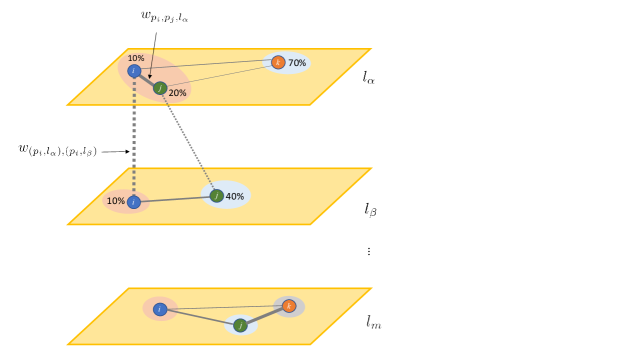
Figure 1: Structure of a MLN with communities generated in each layer.

Nodes are represented by dots of different colors, and they may be present in all or only a subset of the layers. Communities are represented by colored circles that surround one or more nodes.

In Figure 1, the edge that connects nodes $p_{i}$ and $p_{j}$ in layer $l_{\alpha}$ is thicker than the ones that connect them to $p_{k}$ in the same layer. This is because these two nodes are more similar between themselves than with $p_{k}$. The score of $p_{i}$ is $10\%$ whereas the score of the $p_{j}$ is $20\%$ in $l_{\alpha}$. Hence, the difference between them, in layer $l_{\alpha}$, is only $10\%$. If we compare the score of $p_{k}$ (of $70\%$), this difference is higher and hence the similarity between $p_{i}$ and $p_{j}$ with $p_{k}$ is lower. The edges are therefore represented by thinner lines.

Since the layers represent different features, the similarity between the same set of entities may differ from layer to layer. An example is illustrated in layers $l_{\alpha}$ and $l_{\beta}$, where the pair of nodes $p_{i}$ and $p_{j}$ have a higher distance between them in $l_{\beta}$ than in $l_{\alpha}$, making the connection between them “weaker”. One of the motivations to use MLNs is the fact that inter-layer edges provide information about the association between features (layers). This association is taken into account when building the communities with a community detection algorithm, by using both intra-layer distances and inter-layer distances for modeling.

The example also illustrates communities generated in each layer, individually. Figure 1 represents a scenario in which a community detection algorithm runs on each single-layer network. In the example, node $p_{i}$ appears in all layers and in the same community, but node $p_{j}$ is assigned to the red community in $l_{\alpha}$ and to the blue community in $l_{\beta}$ and in $l_{m}$. Additionally, node $p_{j}$ is assigned to the same community as $p_{i}$ in $l_{\alpha}$, but to other communities in the other layers. We assume that if the community structure of layers are heterogeneous, then they provide different information about the nodes (patients). These three layers could then be considered as not redundant with respect to its community structure.

As previously mentioned, using a bi-directional metric for layer similarity is crucial in the context of the current work, due to the fact that ground-truth is unknown. For instance, if we compare the red community in $l_{\alpha}$ to the red community in $l_{m}$ and use the $l_{\alpha}$ as the ground truth, then its precision and recall is $1$ and $\frac{1}{2}$, respectively. For the blue community, precision and recall are both $0$. If we compute the weighted sum of the precision and recall, then this results in $\frac{1}{2}$ of precision and $\frac{1}{4}$ of recall. Therefore, the F-measure ($F^{[l_{\alpha}\|l_{m}]}$) over all communities is $\frac{1}{3}$. In contrast, when we consider $l_{m}$ as the ground-truth, then the precision and recall for the red community are, respectively, $\frac{1}{2}$ and $1$. For the blue community, both values are $0$. In this case, we also include the grey community and compute its precision and recall, which is $0$ for both values. The weighted average of the recall, for this community solution, is $\frac{1}{6}$ and of the precision is $\frac{1}{3}$. The F-measure ($F^{[l_{m}\|l_{\alpha}]}$) is then $\frac{2}{9}$. As a result, there is a significant difference when one layer is assumed to be the ground-truth solution versus the other.

4.5 Cost-Based Layer Selector – COBALT

On the basis of the aforementioned cost model, we now present our algorithm COBALT for cost-based layer selection and community construction.

Table 3 displays a description of the main variables used in the pseudocodes that follow.

Symbol	Description
$G$	set of graphs
$\mathcal{S}_{single}$	set of the community memberships (partitions) of the nodes for each of the single-layer networks $g\in{}G$
$g_{bestsingle}$	first graph chosen for the MLN, it contains the partition with the best modularity
$S_{bestsingle}$	partition of the first graph
$\mathcal{L}$	the network structure: a single-layer or multi-layer network

Table 3: Notation table

Algorithm 1 shows the pseudocode for the generation of the starting solution.

Algorithm 1 COBALT Initialization: Pseudo code for choosing the first layer

1:$G$

2:$g_{bestsingle}$

3:$\mathcal{S}_{single}\leftarrow\emptyset$

4:$g_{bestsingle}\leftarrow\mathit{NULL}$

5:$S_{bestsingle}\leftarrow\mathit{NULL}$; $q_{bestsingle}\leftarrow-\infty$

6:for $g\in G$ do

7:     $(S,q)\leftarrow\mathit{Leiden}(g)$

8:     $\mathcal{S}_{single}\leftarrow\mathcal{S}_{single}\cup\{S\}$

9:     if $q_{bestsingle}<q$ then

10:         $g_{bestsingle}\leftarrow g$

11:         $S_{bestsingle}\leftarrow S$ ; $q_{bestsingle}\leftarrow q$

12:     end if

13:end for

14:return $g_{bestsingle},S_{bestsingle},\mathcal{S}_{single}$

The input of Algorithm 1 is the set of all single-layer graphs $G$. For each $g\in{}G$, COBALT invokes the Leiden algorithm which builds a set of communities and returns two objects: the ‘partition’ $S$, which encompasses the community membership of each node for the incumbent graph $g\in G$, and $q$ – the modularity of $S$. The partition $S_{bestsingle}$ with the largest modularity and the corresponding graph $g_{bestsingle}$ are returned as initial solution of COBALT, together with the set of all single-layer partitions.

After the initialization, COBALT gradually adds layers to build up a multi-layer network and derive the best set of communities in it. In each iteration, it invokes the cost model (cf. subsection 4.3) to add the least-cost layer, until a stopping criterion is met. The pseudocode is depicted in Algorithm 2. Note that we consider the first iteration of Algorithm 2 as iteration 2, since the iteration 1 represents Algorithm 1.

Algorithm 2 Iterative Layer Selection: Pseudo-code of the subsequent iterations of COBALT

1:$G,g_{bestsingle},S_{bestsingle},\mathcal{S}_{single}$

2:$S_{best}$ (best set of communities)

3:$G_{candidates}\leftarrow G\setminus\{g_{bestsingle}\}$

4:$S\leftarrow S_{bestsingle}$

5:$\mathcal{L}\leftarrow g_{bestsingle}$

6:while $G_{candidates}\neq\emptyset$ and SC is False do

7:     $g\leftarrow{}\mathit{NULL}$; $c\leftarrow{}+\infty$

8:     for $u\in G_{candidates}$ do

9:         $c_{u}\leftarrow cost(\mathcal{L},u,S,S_{u})$

10:         if $c_{u}<c$ then

11:              $g\leftarrow{}u$ ; $c\leftarrow{}c_{u}$

12:         end if

13:     end for

14:     extend $\mathcal{L}$ with $g$

15:     $(S_{\mathcal{L}},q_{\mathcal{L}})\leftarrow Leiden(\mathcal{L})$

16:     $G_{candidates}\leftarrow G_{candidates}\setminus\{g\}$

17:end while

18:return $S_{\mathcal{L}}$

The input of Algorithm 2 is the set of single-layer graphs $G$ and the outputs of Algorithm 1. The graph $g_{bestsingle}$ becomes the first layer of the MLN structure $\mathcal{L}$, which is built iteratively by adding layers. To expand $\mathcal{L}$, the list of candidate graphs $G_{candidates}$ is created from $G$ and is dynamically updated to remove the graph $g$ added at each iteration. To choose this graph $g$, the layer cost is computed for each candidate $u\in G_{candidates}$, using the cost formula of Eq. 8.

This computation is made between the candidate $u$ and $\mathcal{L}$, but it demands also the community memberships (for the community similarity term). To make this more clear, we include the corresponding partitions.

Next, the least-cost candidate $g$ is selected. $\mathcal{L}$ is expanded to incorporate $g$ and the inter-layer edges between its nodes and the nodes in $g$. Then, the set of communities is built, $G_{candidates}$ is updated and the next iteration starts.

The algorithm runs while there are candidates in $G_{candidates}$ and while the stopping condition SC is false. The stopping condition monitors the cost of the growing MLN, and is specified in the next subsection 4.6.

4.6 Stopping condition for COBALT

The main loop of COBALT (cf. Algorithm 2, while-loop) gradually adds each layer; the cost function only decides which layer to add next. Since layers are chosen on the basis of availability ratio and community similarity (Eq. 2), and since both factors take positive values, cost cannot be negative. Availability ratio may increase or drop from one iteration to the next, though. Two stopping criteria can be derived from it:

• SC1: COBALT stops when the availability ratio decreases towards the previous iteration

• SC2: COBALT stops when the availability ratio drops and the community similarity increases

where the ‘previous iteration’ is the 2nd (i.e. the 1st after the initialization) or a later one.

We choose SC1 as stopping condition in the while-loop. In our experiments, SC1 is not used, because we study the behavior of COBALT as each layer is added. We rather report at which iteration COBALT would have stopped, and what would have been the effect on the communities’ contribution to predictive power.

5 Evaluation design

For the evaluation of COBALT, we use modularity as internal measure and contribution to predictive performance as external measure. We further quantify the impact of missingness.

5.1 Phenotype quality as modularity

To investigate the role of layer cost on phenotype quality, we use modularity as community quality evaluation measure, cf. formula in Eq. 3 and we study how modularity changes as layers are added in a cost-sensitive way.

5.2 Community visualization scheme

To acquire insights on how communities change after selecting each additional layer, we use the Fruchterman-Reingold layout Fruchterman and Reingold (1991) as basis for visualization: nodes that are positioned closer to one another have stronger connections between them than with the ones located far apart. In this layout, we use colors for the communities, i.e. each node takes the color of the community it belongs to. Thus, ‘good’ communities are visualized as graph partitions colored with only one color, while the occurrence of multiple colors in one area of the visualized network indicates that the communities are mixed up.

Since the Fruchterman-Reingold layout is two-dimensional, we place the visualizations of the layers used in each iteration for community detection next to each other; thus, we can see how the colors/communities span across layers.

5.3 Measuring the contribution of phenotypes to predictive quality

To assess the contribution of the phenotypes discovered by COBALT towards phenotype-sensitive treatment, we first build a ‘Baseline’ set of regressors, each of which predicts the score of each questionnaire (layer) at $t_{1}$. They use the following features for each patient: age, gender and score of that questionnaire at $t_{0}$. We compare this ‘Baseline’ to regressors that also exploit community information, namely the ID of the patient’s community for each patient/layer node. Since the patient’s community changes as layers are added by COBALT, we train one regressor on the community augmented data for each iteration.

For regression we use linear regressor, ridge, LASSO and SVR (support vector regressor). To set the hyperparameters, we apply a grid search. We perform 10-fold cross validation, and we evaluate with mean absolute error (MAE), mean squared error (MSE) and $R^{2}$.

By using the post-treatment score (at $t_{1}$) of each layer as target and the communities at each iteration as input, we also assess to what extent we can predict a post-treatment score for some layer without exploiting the pre-treatment data (at $t_{0}$) of this layer. In particular, assume that the post-treatment score of questionnaire/layer $l$ is used as target and that we use as input the communities learned over the layers $l_{1}$ (first iteration) and $l_{2}$ (second iteration), where $l\not\in\{l_{1},l_{2}\}$. If the prediction quality is high in the evaluation setting for a given phenotype, then we expect that we can predict the score of $l$ at $t_{1}$ without recording layer $l$ for this phenotype at all.

Lastly, we compare the contribution to predictive quality achieved by the communities found by COBALT to the predictive quality achieved when using clusters built with traditional clustering algorithms. The clustering techniques used are: (i) agglomerative hierarchical clustering Day and Edelsbrunner (1984), which we denote as ‘AHS’; (ii) BIRCH Zhang et al. (1996), (iii) Gaussian Mixture Models with the Expectation Maximization algorithm Biernacki et al. (2000); Dempster et al. (1977), which we denote as ‘GMM_EM’; (iv) HDBSCAN Campello et al. (2015), (v) k-means Hartigan and Wong (1979) and (vi) OPTICS Ankerst et al. (1999). It must be stressed that these clustering models serve only as baselines, because they operate under different conditions than COBALT: they are cost-insensitive, since they exploit all questionnaires/layers, while COBALT uses only the layers up to a given iteration. Moreover, these clustering algorithms do not handle missing values, hence they are trained only on patients that answered all the questionnaires.

5.4 Measuring how missingness affects phenotype quality

COBALT is designed to deal with layers that contain only few nodes, i.e. layers for which only few entities (in our application: patients) have delivered data. To measure the influence of missingness, we gradually introduce missingness into a dataset that originally has no missing data. In this dataset, when removing an entity, we remove its corresponding node from all layers.

The complete workflow is as follows. If the dataset in use contains missing values, we extract from it the subset $D$ that has no missing values. In the next step, we specify the maximum and minimum of the ‘missingness ratio’, which we define the percentage of entities to be randomly selected and eliminated from $D$. Next, we perform a grid search between the minimum and maximum percentage and derive the corresponding subset of $D$ for each value in the grid; for our experiment, we vary the missingness ratio from $0.1$($10\%$ of entities removed) to $0.9$($90\%$ of the entities removed), with a step of $0.1$, i.e. of 10%. Finally, we run COBALT on each derived dataset and measure quality as (i) modularity at each iteration and (ii) predictive quality for the iteration with the best modularity.

6 Results and Discussion

For our evaluation, we apply COBALT on the tinnitus patient dataset described in section 3. This dataset contains 5 questionnaires: in a realistic scenario, the addition of layers would have stopped at an upper boundary of cost/budget; for the evaluation, we add all layers and study the effects of adding each one. COBALT adds the layers in the following order: (1) THI, (2) MDI, (3) TQ, (4) TBF12 and (5) TFI questionnaire. This indicates that the benefit of adding THI is the highest and the benefit of adding TFI is low.

6.1 Modularity vs cost per iteration

Figure 2 shows the evolution of the modularity $Q$ per iteration, as well as the layer cost and availability ratio of the selected layer at that iteration.

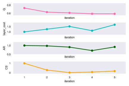
Figure 2: Evolution of modularity (uppermost subfigure), cost (middle upper subfigure), availability ratio (middle lower subfigure) and community similarity (lowermost subfigure), computed as layers are added by COBALT, one at a time.

The modularity decreases as layers are added (uppermost subfigure), while the community similarity stagnates at 0 (lowermost subfigure), indicating that there is substantial difference among the communities built while adding layers. Despite the decrease in modularity, it is important to note that the drop is from $0.730$ to $0.591$, indicating that there are underlying structures in the MLN. The visualizations presented next deliver insights on how communities change as layers are added.

At the same time, the cost of adding a layer is increasing for all but the 4th layer (cf. middle upper subfigure). This increase is mostly due to the decrease in the availability ratio (cf. middle lower subfigure), since community similarity is always low. The availability ratio decreases slowly, hence SC1 can be triggered already at the 3rd or at the 4th iteration.

6.2 Community visualization

In Figures 3 to 8 we show the communities as COBALT adds layers. The visualization is two-dimensional and therefore we show one subfigure per layer.

6.2.1 Visualization of one layer

In Figure 3 we depict the 6 communities in the THI layer, which is chosen by COBALT in the first iteration.

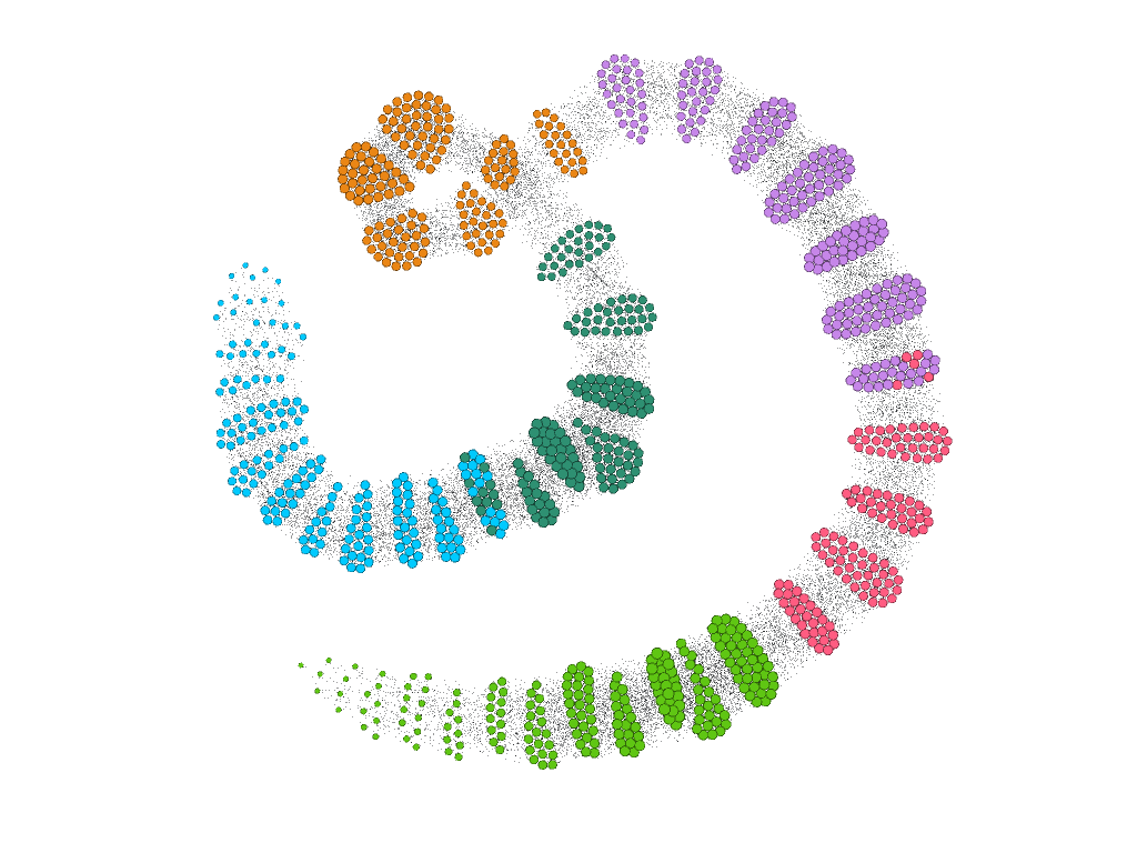
Figure 3: 1st iteration: 6 communities on the THI network; $Q=0.730$. Different colors represent different communities.

The communities mark areas of a single color. There is one subgraph with nodes of the ‘blue’ and the ‘darkgreen’ communities, and one subgraph with both ‘purple’ and ‘pink’ nodes, but these two subgraphs are only small parts of the network. Hence, the visualization scheme captures properly community separation and clearly marks the areas with nodes from more than one community.

Score distributions

Figure 4 depicts the distribution of the questionnaire scores for each of the 6 communities of this 1st iteration of COBALT.

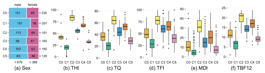
Figure 4: The 6 communities of the THI network added by COBALT as 1st layer, depicting the value distributions inside each questionnaire.

The first column of Figure 4 shows the value distribution for sex, with one row per community. Subsequently, we show one column per questionnaire and, inside it, one boxplot per community. We see that all communities are rather homogeneous with respect to the THI questionnaire: the small boxes indicate small variance. The variance increases for the other questionnaires; this is expected, since COBALT considered only the THI data to build these communities.

There are remarkable differences among some of the communities. Community C1 (green boxes for the questionnaires) has the lowest average value in each questionnaire, while community C2 (fade-yellow boxes) has the highest average values, indicating C1 and C2 have considerably different characteristics. In the context of the data used, it seems that C1 accommodates the patients with the most mild tinnitus symptoms, while C2 accommodates the patients with the most severe tinnitus symptoms.

6.2.2 Communities across layers

Figure 5 depicts the 5 communities found in the 2nd iteration, where COBALT adds the MDI layer as the one with the lowermost cost.

(a) THI network

(b) MDI network

Figure 5: 2nd iteration with MDI questionnaire as 2nd layer: 5 communities detected; $Q=0.632$.

As we have seen in the evolution curves of Figure 2, iteration 2 incurs a cost increase and a slight modularity drop. The visualization of the communities in the two layers makes this evident: there is a rather clear separation of colors in the THI network (cf. subfigure 5(a)), but the colors in the MDI network (cf. subfigure 5(b)) are mixed. Hence, the use of the inter-layer similarities and the similarities inside the MDI network did not contribute to a good modularity score.

Figure 6 shows the 4 communities found in the 3rd iteration, where COBALT added the TQ layer. From this iteration on, community induction is driven by the node similarities inside the MDI layer, leading to more homogeneous communities in the MDI layer, while the community colors in the other layers are mixed.

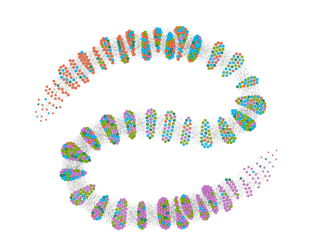
(a) THI network

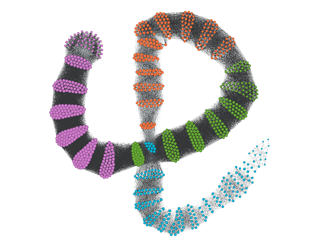
(b) MDI network

(c) TQ network

Figure 6: 3rd iteration with TQ questionnaire added as 3rd layer: 4 communities detected; $Q=0.613$.

A further remarkable aspect in Figure 6 is the high density of the MDI network: the patients are very similar to each other inside this layer. This might have led to communities that are not clearly separated. This can also be seen in Figure 7, which depicts the 4 communities found when COBALT adds TBF12 as 4th layer.

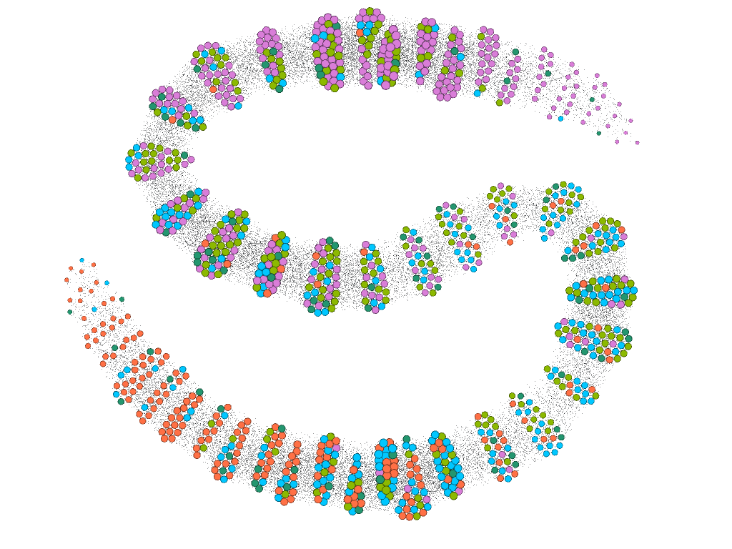
(a) THI network

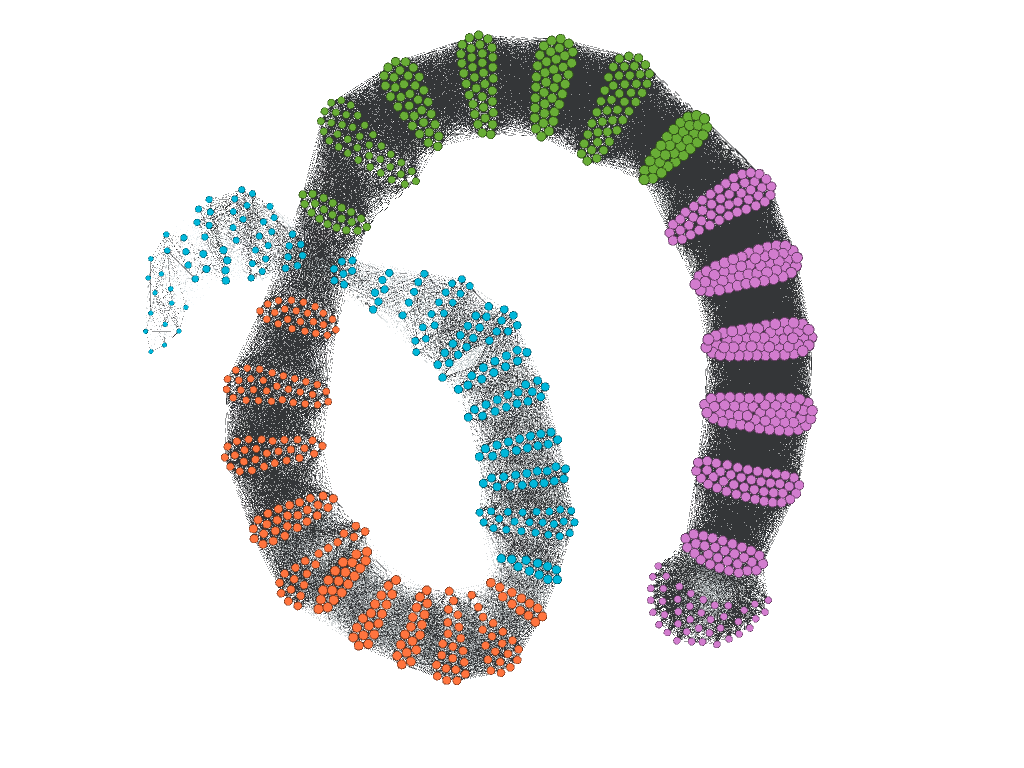
(b) MDI network

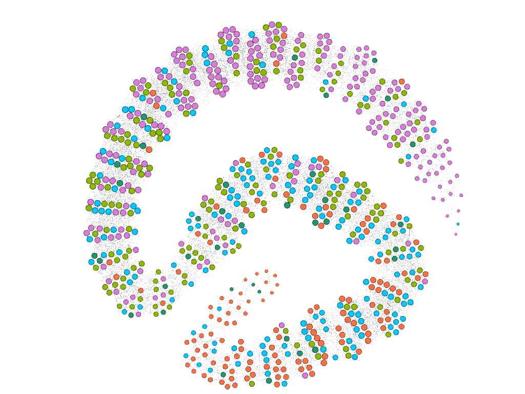
(c) TQ network

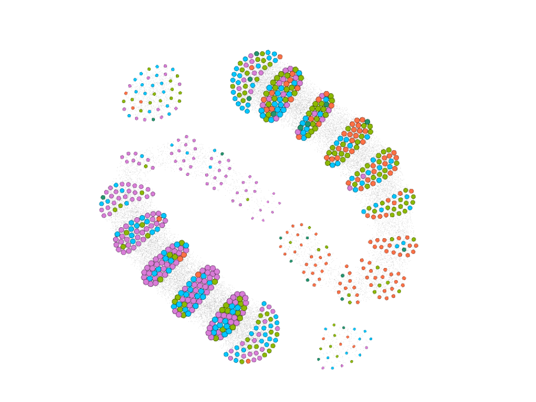
(d) TBF12 network

Figure 7: 4th iteration with TBF12 added as 4th layer: 4 communities detected; $Q=0.592$.

As in the 3rd iteration, nodes are well-separated into communities with respect to the MDI layer, but not with respect to the other layers. The number of communities is also the same as before: although this does not imply that the communities are exactly the same, it indicates adding the TBF12 layer does not add much information to the previous MLN.

Finally, Figure 8 shows the 4 communities found in the 5th iteration, when the TFI layer is added as last one.

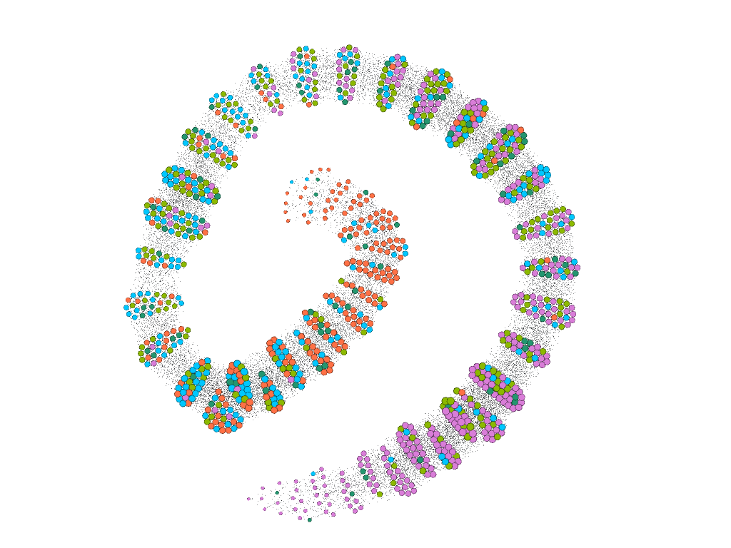
(a) THI network

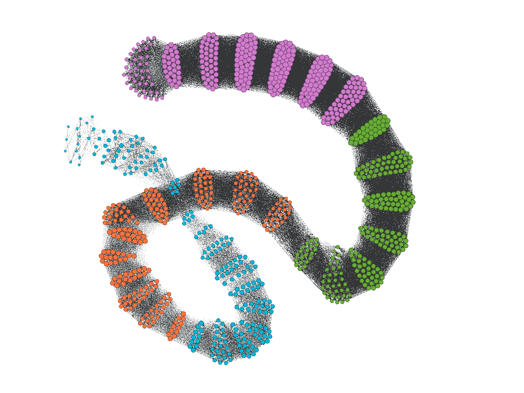
(b) MDI network

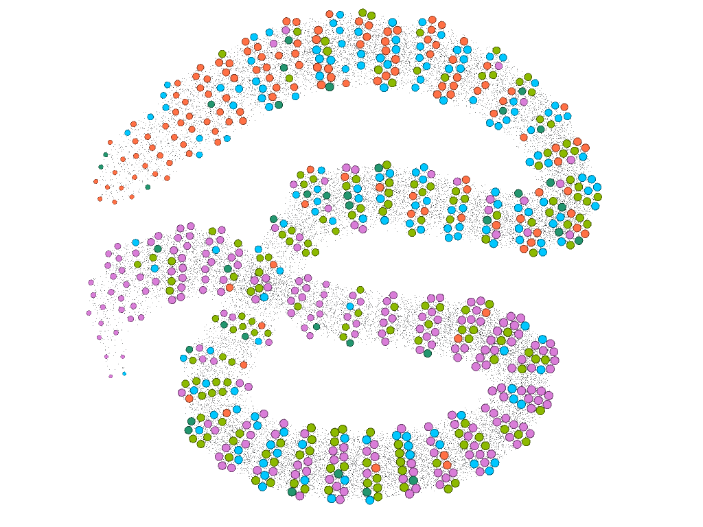
(c) TQ network

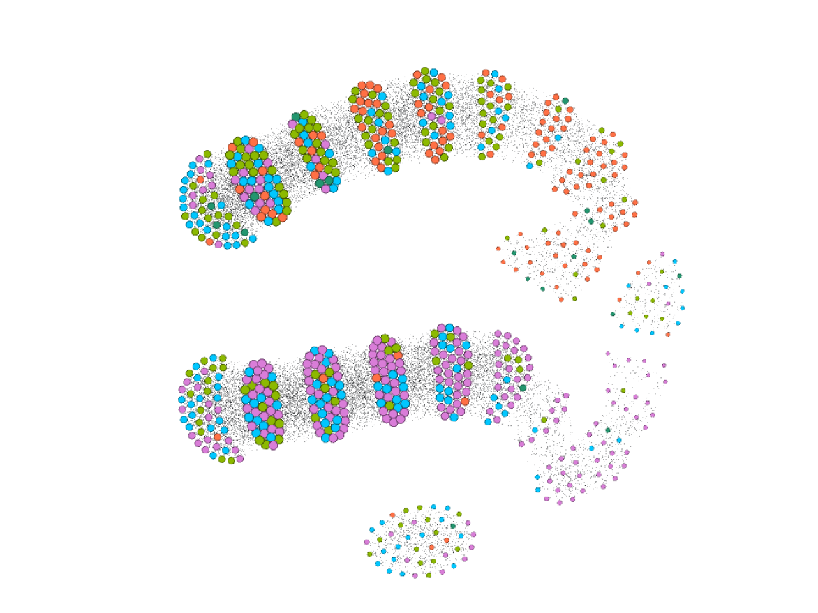
(d) TBF12 network

(e) TFI network

Figure 8: 5th iteration, last layer (TFI) added: 4 communities detected; $Q=0.591$.

As before, the communities are well separated in the MDI network, but not in the other networks. The modularity ($0.591$) is also very close to the modularity value of the 4th iteration ($0.592$).

Summarizing, the visualization scheme shows a deterioration of community quality as layers are added. The evolution of layer cost and of its two factors capture this deterioration well; the SC1 stopping criterion would have stopped the MLN expansion after the 3rd iteration by the latest.

In our application scenario, communities serve as phenotypes, intended to contribute to prediction. For that reason, we next report on how the communities contributed to predictive quality.

6.3 Phenotypes for prediction

According to our evaluation design, we compare the prediction quality achieved when using COBALT communities to that achieved by the Baseline regressors and to the quality achieved when using clustering instead of COBALT.

The results are on Table 4, which we discuss in detail hereafter. For each of the 5 scores at $t_{1}$, we depict the performance as MSE and MAE (where smaller values are better) and $R^{2}$ (where larger values are better). Values marked in boldface are the best achieved for predicting a questionnaire score.

	Partition quality		THI score at $t_{1}$			MDI score at $t_{1}$			TQ score at $t_{1}$			TBF12 score at $t_{1}$			TFI score at $t_{1}$
Model	silhouette	Q	MSE	MAE	$R^{2}$	MSE	MAE	$R^{2}$	MSE	MAE	$R^{2}$	MSE	MAE	$R^{2}$	MSE	MAE	$R^{2}$
Baseline			$13.1$	$287.6$	$0.569$	$5.1$	$43.0$	$0.686$	$9.9$	$159.9$	$0.394$	$3.1$	$13.2$	$0.182$	$10.2$	$158.4$	$0.637$
COBALT
iteration 1		0.730	9.3	130.9	0.720	4.9	43.0	0.707	$11.3$	$280.3$	$0.284$	$2.8$	$13.2$	$0.613$	11.1	$346.4$	$0.344$
iteration 2		0.632	$12.3$	$228.2$	$0.439$	$5.4$	$62.6$	$0.532$	$9.6$	$143.4$	$0.521$	$2.4$	$9.8$	$0.798$	10.1	148.2	0.730
iteration 3		0.613	$9.6$	$154.6$	$0.563$	$6.2$	$75.4$	$0.227$	$9.2$	$123.7$	$0.573$	2.1	5.9	0.866	$13.1$	$294.2$	$0.354$
iteration 4		$0.592$	$13.0$	$265.8$	$0.606$	4.4	36.9	0.715	$7.6$	$93.9$	$0.622$	$2.5$	$8.7$	$0.738$	$11.2$	$177.9$	$0.621$
iteration 5		$0.591$	$8.6$	$103.5$	$0.748$	$5.9$	$68.7$	$0.302$	$11.6$	$227.1$	$0.379$	$3.2$	$13.4$	$0.595$	$14.9$	$356.8$	$0.359$
Clusterers
AHC	$0.479$		$9.9$	$198.9$	$0.565$	$8.8$	$116.8$	$0.203$	$8.2$	$110.2$	$0.355$	$2.1$	$6.4$	$0.765$	$14.8$	$389.3$	$-0.085$
BIRCH	$0.482$		$10.1$	$183.1$	$0.576$	$5.3$	$53.6$	$0.599$	$6.7$	$61.5$	$0.455$	$3.8$	$15.7$	$0.671$	$11.7$	$325.6$	$0.108$
GMM_EM	$0.349$		$8.4$	$138.5$	$0.564$	$6.8$	$82.1$	$0.545$	5.6	40.4	0.758	$3.4$	$12.7$	$0.752$	$12.3$	$213.1$	$0.557$
HDBSCAN	$0.134$		$11.7$	$216.5$	$0.738$	$5.6$	$59.2$	$0.572$	$10.6$	$195.0$	$0.520$	$3.0$	$9.4$	$0.318$	$16.7$	$533.9$	$0.095$
k-means	$0.481$		8.2	107.2	0.883	$5.4$	$53.9$	$0.370$	$9.1$	$140.4$	$0.735$	$2.5$	$8.9$	$0.777$	$16.0$	$415.3$	$0.309$
OPTICS	$0.406$		$9.1$	$148.4$	$0.650$	3.8	21.2	$0.704$	$10.4$	$166.6$	$0.458$	$4.1$	$20.2$	$-4.564$	$10.7$	$184.4$	$0.410$

Table 4: Prediction of questionnaire scores at $t_{1}$ given age, gender, score at $t_{0}$ (Baseline, first row of values) and, additionally the phenotype IDs returned by COBALT (upper part), respectively by the clustering algorithms (lower part); for convenience, we ordered the columns with the same order as layers were added by COBALT, but this ordering has no effect on the way the data are read by the predictor.

6.3.1 Prediction with the phenotypes of each COBALT iteration

The upper part of Table 4 shows for each iteration of COBALT (first column) the quality of the phenotypes in the MLN network, measured as modularity Q (third column). For each predicted score, we mark in underline the best values achieved in a COBALT iteration.

For each score, the COBALT-augmented regressor outperforms the corresponding Baseline regressor, as can be seen by the underlined values for the scores. When focusing on the phenotypes of each iteration, we observe the following:

• iteration 1: COBALT outperforms the Baseline for the THI score and for the MDI and TBF12 scores (the MAE values are identical). For the TQ and TFI scores, the Baseline is better.

• iteration 2: COBALT outperforms the Baseline for the TQ, TFI and TBF12 scores. For the THI score, COBALT is better with respect to MSE and MAE. For the MDI score, COBALT is inferior than the Baseline. This is remarkable, since the layer included in the 2nd iteration is the MDI layer itself. However, as can be seen in Figure 5, the communities are more oriented towards THI.

• iteration 3: COBALT outperforms the Baseline for the TQ and TBF12 scores, and for the THI score with respect to MSE and MAE. With respect to the MDI score and the TFI score, the Baseline is superior.

• iteration 4: COBALT outperforms the Baseline for the THI, MDI, TQ and TBF12 scores, i.e. all but the TFI score.

• iteration 5: COBALT outperforms the Baseline for the THI score, but it is inferior to it for all the other scores.

Summarizing, the COBALT phenotypes on the THI and MDI layers suffice to predict 4 out of the 5 scores at $t_{1}$ with better MAE and MSE than the Baseline that exploits the scores of all 5 questionnaires at $t_{0}$. The phenotypes of the THI layer alone suffice for predicting 3 out of 5 scores at $t_{1}$. This indicates that the exploitation of phenotypes during prediction is advantageous, and the advantage is higher when adding the least-cost layer.

The influence of the MDI layer must be perceived as an artifact, since this layer improves predictive performance but not for the MDI score itself An explanation is in the density of this layer, which may have resulted in poor-quality communities inside this layer.

6.3.2 COBALT vs clustering

The lower part of Table 4 depicts the prediction quality achieved when using clustering algorithms for phenotype construction instead of COBALT on MLNs. We varied the number of clusters to optimize silhouette, and we report the clusters found for this optimal number. For example, for k-means, the best silhouette was for $k=2$.

For each of the 5 scores there is at least one clustering algorithm that outperforms the Baseline (first row). As with COBALT, this indicates that exploiting phenotypes during prediction is of advantage. However, unlike COBALT, there is no clear winner among the clustering algorithms: for the THI score, all algorithms delivered models that were superior to the Baseline; for the TFI score, none did; for the other scores, some models were superior to the Baseline and others were inferior to it.

COBALT outperforms the Clustering approaches when predicting the TFI score (iteration 2) and the TBF12 score (iteration 3), i.e. before the corresponding layers are added. For the MDI score, iteration 4 delivers the best $R^{2}$ value, but is inferior to OPTICS with respect to MSE and MAE. For the THI score, K-Means returns the best results. However, there is no clear winner among the Clustering approaches with respect to phenotype contribution: for each of the 5 scores, another algorithm is best for one or more of the three measures, although, unlike COBALT, all Clustering algorithms are trained on all scores at $t_{0}$. In contrast, the phenotypes returned by COBALT on the first two layers outperform the Baseline for all scores except the MDI.

COBALT and Clustering cannot be compared directly on community homogeneity: for clustering, we use silhouette instead of modularity. When juxtaposing the results of the Clustering algorithms, we see that BIRCH returns the phenotypes with the highest silhouette value, but these phenotypes contribute less to prediction than those output by other clustering algorithms. This agrees with our observation on modularity for COBALT: the phenotypes returned at iteration 1 have the highest modularity but the regressors exploiting them are of inferior quality.

Summarizing, the phenotypes returned by COBALT exhibit more consistent predictive performance than achieved by clusters built by individual clustering algorithms, albeit the latter exploit all scores at $t_{0}$. This holds particularly for iteration 2, where a layer is chosen in a cost-sensitive way, before the stopping criterion SC1 is triggered. Phenotype quality, either the modularity in MLNs or the silhouettes in clustering, are poor indicators of predictive performance. For COBALT, phenotypes built in a cost-sensitivity way lead to competitive predictive performance.

6.3.3 COBALT vs cost-insensitive MLN phenotypes

In our earlier work Puga et al. (2021), we built MLN-based phenotypes, optimizing on modularity rather than cost. Table 5, from Puga et al. (2021), shows the layer selected at each iteration and the modularity scores achieved.

	Layers	Q
iteration 1	THI	0.752
iteration 2	[THI, TQ]	0358
iteration 3	[THI, TQ, TBF12]	0.362
iteration 4	[THI, TQ, TBF12, TFI]	0.002
iteration 5	[THI, TQ, TBF12, TFI, MDI]	0.001

Table 5: From Puga et al. (2021): Modularity per iteration.

When we compare with the column on $Q$ of Table 4, we see that COBALT achieves higher modularity values. This can be explained by the differences in the data: albeit we use the same dataset and prediction tasks, in Puga et al. (2021) we considered only patients that had available data in all layers, whereas COBALT uses all data, allowing for missing values in some layers.

A comparison on prediction quality is not possible because in Puga et al. (2021) we predicted for each community separately, and only for the TQ score at $t_{1}$, considering only communities that had enough data for learning and testing. Nonetheless, we can state that COBALT is superior to the predecessor approach of Puga et al. (2021) by design, since it allows for missing values.

6.4 Impact of missingness

Figure 9 shows how modularity changes from the 1st to the last iteration as we increase missingness from 10% (leftmost, uppermost subfigure) to 90% (rightmost, lowermost subfigure) in steps of percentual points. The data with 0% missingness lead to the modularity values depicted by the dashed line in each of the subfigures.

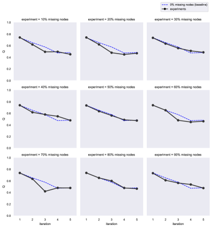
Figure 9: Modularity per iteration as missingness ratio is increased from 10% to 90%.

	Partition quality	THI score at $t_{1}$					MDI score at $t_{1}$					TQ score at $t_{1}$
	Q (best)	n	NL	MSE	MAE	$R^{2}$	n	NL	MSE	MAE	$R^{2}$	n	NL	MSE	MAE	$R^{2}$
Ratio of node missingness
$0\%$	$0.740$	$48$	$1$	$8.0$	$102.3$	$0.850$	$47$	$1$	$7.1$	$90.0$	$0.601$	$29$	$1$	$7.5$	$88.6$	$0.703$
$10\%$	$0.741$	$48$	$4$	$9.1$	$149.0$	$0.789$	$47$	$1$	$5.5$	$45.4$	$0.574$	$29$	$1$	$9.8$	$142.5$	$0.635$
$20\%$	$0.742$	$48$	$4$	$7.9$	$89.9$	$0.847$

Table 6: Prediction quality for each percentage value of missingness, showing the iteration (equiv. number of layers NL) that achieves the best modularity.

The curves indicate that the modularity is not greatly affected by missingness: it always drops towards 0.4, it always remains close to the reference (dashed) line of 0% missingness, mostly a bit below it but sometimes above it. These findings suggest that subsets of the nodes in the MLN have intra/inter-layer edges and weights that lead to communities of comparable quality to that of 0% missingness. Table 6 depicts prediction quality as we increase missingness from 0% to 10% and then to 20%. Prediction was possible only for THI, MDI and TQ scores at $t_{1}$ when the missingness was 0% and 10%, and only for THI when the missingness was increased to 20%. For TFI and TBF12, there were not enough data for training and testing. For each missingness value we chose the iteration with the highest modularity: this is reflected in the column ‘NL’ that denotes the Number of Layers (NL) used and may differ depending on the questionnaire score being predicted. The number of patients used for training is shown in the column marked as ‘n’, which again may differ for each questionnaire score.

In Table 4 we have seen that a decrease in modularity is not necessarily associated with a tendency in the values of the prediction quality measures. This agrees with the results in Table 6, where the sets of communities with the best modularity are chosen but the prediction quality measures vary in both directions. In general, the prediction quality is good, which indicates that a small increase in missingness does not lead to dramatic quality deterioration. However, the amount of training data is so small that a generalization is not possible.

7 Conclusion

In this work we have presented COBALT, a cost-based model to find communities in a single- or multi-layer network structure. We define cost as the cost of acquiring features and test it in a dataset with questionnaire data from chronic tinnitus patients. We also compare our results with traditional clustering methods.

The major findings of this work can be summarized into four:

1. COBALT is able find partitions in the data that are superior to conventional clustering algorithms in terms of our evaluation criteria (performance on post-treatment data prediction) for three of the five questionnaire predictions;

2. COBALT outperforms our prior work with the same dataset (cf. Puga et al. (2021)) by achieving higher modularity values. As a result, taking a cost-effective strategy and allowing missing values in each layer proved advantageous;

3. The partitions with the best modularity do not lead necessarily to the best inputs for a post-treatment data predictor;

4. Missing values have no substantial impact on the modularity of the partitions.

In the context of clinical decision support, COBALT is intended for personalized diagnostics and treatment planing on the basis of patient phenotypes. COBALT demonstrates that it is possible to build predictive phenotypes without demanding a large number of questionnaires, as was the case in our earlier work Niemann et al. (2020). Our approach can be used in different ways. First, we have shown that phenotypes are predictive; hence, once a patient’s phenotype has been assessed, treatment outcome can be predicted without demanding that the patient fills further questionnaires. Thus, the burden of the patient during the diagnostic procedure can be reduced. Next, the acquisition of information during screening can be focused towards informative features, thus reducing cost without compromising quality. Finally, phenotype-specific treatments can be designed. To this purpose, clinical research is needed to assess the robustness of the identified models and their predictiveness. Moreover, the cost-sensitive selection of questionnaires and the usage of phenotypes in the clinical practice demand a modification of the diagnostic guidelines, which, again, is best initiated with a prospective study.

Funding

This project has received funding from the European Union’s Horizon 2020 Research and Innovation Programme under grant agreement number 848261.

Conflict of interest statement

The authors declare no conflict of interest.

References

- Ric [2016] A survey of clinical phenotyping in selected national networks: demonstrating the need for high-throughput, portable, and computational methods. Artificial Intelligence in Medicine, 71:57–61, 2016. ISSN 18732860. 10.1016/j.artmed.2016.05.005.
- Ali et al. [2019] Hafiz Tiomoko Ali, Sijia Liu, Yasin Yilmaz, Romain Couillet, Indika Rajapakse, and Alfred Hero. Latent Heterogeneous Multilayer Community Detection. In ICASSP 2019 - 2019 IEEE International Conference on Acoustics, Speech and Signal Processing (ICASSP), pages 8142–8146. IEEE, may 2019. ISBN 978-1-4799-8131-1. 10.1109/ICASSP.2019.8683574.
- Alimadadi et al. [2019] Fatemeh Alimadadi, Ehsan Khadangi, and Alireza Bagheri. Community detection in facebook activity networks and presenting a new multilayer label propagation algorithm for community detection. International Journal of Modern Physics B, 33(10):1950089, apr 2019. ISSN 0217-9792. 10.1142/S0217979219500899.
- Amanat et al. [2020] Sana Amanat, Teresa Requena, and Jose Antonio Lopez-Escamez. A systematic review of extreme phenotype strategies to search for rare variants in genetic studies of complex disorders. Genes, 11(9):1–15, 2020. ISSN 20734425. 10.3390/genes11090987.
- Ankerst et al. [1999] Mihael Ankerst, Markus M Breunig, Hans-Peter Kriegel, and Jörg Sander. Optics: Ordering points to identify the clustering structure. ACM Sigmod record, 28(2):49–60, 1999.
- Bech et al. [2001] P. Bech, N.-A. Rasmussen, L.Raabæk Olsen, V. Noerholm, and W. Abildgaard. The sensitivity and specificity of the major depression inventory, using the present state examination as the index of diagnostic validity. Journal of Affective Disorders, 66(2-3):159–164, 2001.
- Biernacki et al. [2000] Christophe Biernacki, Gilles Celeux, and Gérard Govaert. Assessing a mixture model for clustering with the integrated completed likelihood. IEEE transactions on pattern analysis and machine intelligence, 22(7):719–725, 2000.
- Bródka et al. [2018] Piotr Bródka, Anna Chmiel, Matteo Magnani, and Giancarlo Ragozini. Quantifying layer similarity in multiplex networks: A systematic study. Royal Society Open Science, 5(8), 2018. ISSN 20545703. 10.1098/rsos.171747.
- Campello et al. [2015] Ricardo JGB Campello, Davoud Moulavi, Arthur Zimek, and Jörg Sander. Hierarchical density estimates for data clustering, visualization, and outlier detection. ACM Transactions on Knowledge Discovery from Data (TKDD), 10(1):1–51, 2015.
- Cima et al. [2012] Rilana FF Cima, Iris H Maes, Manuela A Joore, Dyon JWM Scheyen, Amr El Refaie, David M Baguley, Lucien JC Anteunis, Gerard JP van Breukelen, and Johan WS Vlaeyen. Specialised treatment based on cognitive behaviour therapy versus usual care for tinnitus: a randomised controlled trial. The Lancet, 379(9830):1951–1959, May 2012. 10.1016/s0140-6736(12)60469-3. URL https://doi.org/10.1016/s0140-6736(12)60469-3.
- Cima et al. [2014] Rilana F.F. Cima, Gerhard Andersson, Caroline J. Schmidt, and James A. Henry. Cognitive-behavioral treatments for tinnitus: A review of the literature. Journal of the American Academy of Audiology, 25(01):029–061, January 2014. 10.3766/jaaa.25.1.4. URL https://doi.org/10.3766/jaaa.25.1.4.
- Day and Edelsbrunner [1984] William HE Day and Herbert Edelsbrunner. Efficient algorithms for agglomerative hierarchical clustering methods. Journal of classification, 1(1):7–24, 1984.
- Dempster et al. [1977] Arthur P Dempster, Nan M Laird, and Donald B Rubin. Maximum likelihood from incomplete data via the em algorithm. Journal of the Royal Statistical Society: Series B (Methodological), 39(1):1–22, 1977.
- Dianati [2016a] Navid Dianati. Unwinding the hairball graph: Pruning algorithms for weighted complex networks. Physical Review E, 93(1), 2016a. ISSN 24700053. 10.1103/PhysRevE.93.012304.
- Dianati [2016b] Navid Dianati. Unwinding the hairball graph: Pruning algorithms for weighted complex networks. Physical Review E, 93(1), 2016b. ISSN 24700053. 10.1103/PhysRevE.93.012304.
- Eggermont and Roberts [2004] Jos J. Eggermont and Larry E. Roberts. The neuroscience of tinnitus. Trends in Neurosciences, 27(11):676–682, 2004. ISSN 01662236. 10.1016/j.tins.2004.08.010.
- Fruchterman and Reingold [1991] Thomas M. J. Fruchterman and Edward M. Reingold. Graph drawing by force-directed placement. Software: Practice and Experience, 21(11):1129–1164, November 1991. 10.1002/spe.4380211102.
- Gao et al. [2019] Xubo Gao, Qiusheng Zheng, Filipe A. N. Verri, Rafael D. Rodrigues, and Liang Zhao. Particle Competition for Multilayer Network Community Detection. In Proceedings of the 2019 11th International Conference on Machine Learning and Computing - ICMLC ’19, volume Part F1481, pages 75–80, New York, New York, USA, 2019. ACM Press. ISBN 9781450366007. 10.1145/3318299.3318320.
- Genitsaridi et al. [2020] Eleni Genitsaridi, Derek J. Hoare, Theodore Kypraios, and Deborah A. Hall. A review and a framework of variables for defining and characterizing tinnitus subphenotypes. Brain Sciences, 10(12):1–21, 2020. ISSN 20763425. 10.3390/brainsci10120938.
- Ghawi and Pfeffer [2022] Raji Ghawi and Jürgen Pfeffer. A community matching based approach to measuring layer similarity in multilayer networks. Social Networks, 68(April 2021):1–14, 2022. ISSN 03788733. 10.1016/j.socnet.2021.04.004.
- Goebel and Hiller [1998] G Goebel and W Hiller. Tinnitus-Fragebogen (TP)-Handanweisung. Hogrefe, Göttingen, 1998.
- Greimel et al. [1999] Karoline V. Greimel, M. Leibetseder, J. Unterrainer, and K. Albegger. Ist Tinnitus meßbar? Methoden zur Erfassung tinnitusspezifischer Beeinträchtigungen und Präsentation des Tinnitus-Beeinträchtigungs-Fragebogens (TBF-12). HNO, 47(3):196–201, 1999.
- Hartigan and Wong [1979] John A Hartigan and Manchek A Wong. Algorithm as 136: A k-means clustering algorithm. Journal of the royal statistical society. series c (applied statistics), 28(1):100–108, 1979.
- Huang et al. [2020] Xinyu Huang, Dongming Chen, Tao Ren, and Dongqi Wang. A survey of community detection methods in multilayer networks. Springer US, 2020. ISBN 1061802000. 10.1007/s10618-020-00716-6.
- Huckvale et al. [2019] Kit Huckvale, Svetha Venkatesh, and Helen Christensen. Toward clinical digital phenotyping: a timely opportunity to consider purpose, quality, and safety. npj Digital Medicine, 2(1), 2019. ISSN 2398-6352. 10.1038/s41746-019-0166-1.
- Interdonato et al. [2020] Roberto Interdonato, Matteo Magnani, Diego Perna, Andrea Tagarelli, and Davide Vega. Multilayer network simplification: Approaches, models and methods. arXiv, (May), 2020. ISSN 23318422.
- [27] Inderjit S Jutla, Lucas GS Jeub, Peter J Mucha, et al. A generalized Louvain method for community detection implemented in MATLAB. URL https://github.com/GenLouvain/GenLouvain(2011-2019).
- Kramer et al. [2020] Jordan Kramer, Lyric Boone, Thomas Clifford, Justin Bruce, and John Matta. Analysis of Medical Data Using Community Detection on Inferred Networks. IEEE Journal of Biomedical and Health Informatics, 24(11):3136–3143, 2020. ISSN 21682208. 10.1109/JBHI.2020.3003827.
- Lee et al. [2020] Bohyun Lee, Shuo Zhang, Aleksandar Poleksic, and Lei Xie. Heterogeneous Multi-Layered Network Model for Omics Data Integration and Analysis. 10(January):1–11, 2020. 10.3389/fgene.2019.01381.
- Liang et al. [2019] Yunji Liang, Xiaolong Zheng, and Daniel D. Zeng. A survey on big data-driven digital phenotyping of mental health. Information Fusion, 52(July 2018):290–307, 2019. ISSN 15662535. 10.1016/j.inffus.2019.04.001.
- McCombe et al. [2001] A. McCombe, D. Baguley, R. Coles, L. McKenna, C. McKinney, and P. Windle-Taylor. Guidelines for the grading of tinnitus severity: the results of a working group commissioned by the british association of otolaryngologists, head and neck surgeons, 1999. Clinical Otolaryngology and Allied Sciences, 26(5):388–393, 2001.
- Meikle et al. [2012] M. B. Meikle, J. A. Henry, S. E. Griest, et al. The tinnitus functional index. Ear & Hearing, 33(2):153–176, 2012.
- Mucha et al. [2010] Peter J Mucha, Thomas Richardson, Kevin Macon, Mason A Porter, and Jukka Pekka Onnela. Community structure in time-dependent, multiscale, and multiplex networks. Science, 328(5980):876–878, 2010. ISSN 00368075. 10.1126/science.1184819.
- Niemann et al. [2020] Uli Niemann, Petra Brueggemann, Benjamin Boecking, Wilhelm Mebus, Matthias Rose, Myra Spiliopoulou, and Birgit Mazurek. Phenotyping chronic tinnitus patients using self-report questionnaire data: cluster analysis and visual comparison. Scientific Reports, 10(1):1–10, 2020. ISSN 20452322. 10.1038/s41598-020-73402-8. URL https://doi.org/10.1038/s41598-020-73402-8.
- Pan et al. [2018] Zhisong Pan, Guyu Hu, and Dong Li. Detecting communities from multilayer networks. In Proceedings of the International Conference on Intelligent Science and Technology - ICIST ’18, pages 6–11, New York, New York, USA, 2018. ACM Press. ISBN 9781450364614. 10.1145/3233740.3233742.
- Puga et al. [2021] Clara Puga, Uli Niemann, Vishnu Unnikrishnan, Miro Schleicher, Winfried Schlee, and Myra Spiliopoulou. Discovery of Patient Phenotypes through Multi-layer Network Analysis on the Example of Tinnitus. 2021 IEEE 8th International Conference on Data Science and Advanced Analytics (DSAA), pages 1–10, 2021. 10.1109/dsaa53316.2021.9564158.
- Rolstad et al. [2011] Sindre Rolstad, John Adler, and Anna Rydén. Response burden and questionnaire length: Is shorter better? A review and meta-analysis. Value in Health, 14(8):1101–1108, 2011. ISSN 10983015. 10.1016/j.jval.2011.06.003.
- Schlee et al. [2021] Winfried Schlee, Berthold Langguth, Rüdiger Pryss, Johannes Allgaier, Lena Mulansky, Carsten Vogel, Myra Spiliopoulou, Miro Schleicher, Vishnu Unnikrishnan, Clara Puga, Ourania Manta, Michalis Sarafidis, Ioannis Kouris, Eleftheria Vellidou, Dimitris Koutsouris, Konstantina Koloutsou, George Spanoudakis, Christopher Cederroth, and Dimitris Kikidis. Using Big Data to Develop a Clinical Decision Support System for Tinnitus Treatment. In Choice Reviews Online, volume 47, pages 175–189. 2021. ISBN 9783030855024. 10.1007/7854_2021_229. URL https://link.springer.com/10.1007/7854_2021_229.
- Tantardini et al. [2019] Mattia Tantardini, Francesca Ieva, Lucia Tajoli, and Carlo Piccardi. Comparing methods for comparing networks. Scientific Reports, 9(1):1–19, 2019. ISSN 20452322. 10.1038/s41598-019-53708-y.
- Traag et al. [2019] V. A. Traag, L. Waltman, and N. J. van Eck. From Louvain to Leiden: guaranteeing well-connected communities. Scientific Reports, 9(1):1–12, 2019. ISSN 20452322. 10.1038/s41598-019-41695-z.
- Yang et al. [2021] Dengcheng Yang, Yi Jin, Xiaoqing He, Ang Dong, Jing Wang, and Rongling Wu. Inferring multilayer interactome networks shaping phenotypic plasticity and evolution. Nature Communications, pages 1–17, 2021. ISSN 2041-1723. 10.1038/s41467-021-25086-5.
- Zhang et al. [1996] Tian Zhang, Raghu Ramakrishnan, and Miron Livny. Birch: an efficient data clustering method for very large databases. ACM sigmod record, 25(2):103–114, 1996.