Particle-Environment Interactions In Arbitrary Dimensions: A Unifying Analytic Framework To Model Diffusion With Inert Spatial Heterogeneities

Abstract

Interactions between randomly moving entities and spatial disorder play a crucial role in quantifying the diffusive properties of a system. Examples range from molecules advancing along dendritic spines, to animal anti-predator displacements due to sparse vegetation, through to water vapour sifting across the pores of breathable materials. Estimating the effects of disorder on the transport characteristics in these and other systems has a long history. When the localised interactions are reactive, that is when particles may vanish or get irreversibly transformed, the dynamics is modelled as a boundary value problem with absorbing properties. The analytic advantages offered by such a modelling approach has been instrumental to construct a general theory of reactive interaction events. The same cannot be said when interactions are inert, i.e. when the environment affects only the particle movement dynamics. While various models and techniques to study inert processes across biology, ecology and engineering have appeared, many studies have been computational and explicit results have been limited to one-dimensional domains or symmetric geometries in higher dimensions. The shortcoming of these models have been highlighted by the recent advances in experimental technologies that are capable of detecting minuscule environmental features. In this new empirical paradigm the need for a general theory to quantify explicitly the effects of spatial heterogeneities on transport processes, has become apparent. Here we tackle this challenge by developing an analytic framework to model inert particle-environment interactions in domains of arbitrary shape and dimensions. We do so by using a discrete space formulation whereby the interactions between an agent and the environment are modelled as perturbed dynamics between lattice sites. We calculate exactly how disorder affects movement due to reflecting or partially reflecting obstacles, regions of increased or decreased diffusivity, one-way gates, open partitions, reversible traps as well as long range connections to far away areas. We provide closed form expressions for the generating function of the occupation probability of the diffusing particle and related transport quantities such as first-passage, return and exit probabilities and their respective means. The strength of an analytic formulation becomes evident as we uncover a surprising property, which we term the disorder indifference phenomenon of the mean first-passage time in the presence of a permeable barrier in quasi 1D systems. To demonstrate the widespread applicability of our formalism, we consider three examples that span different spatial and temporal scales. The first is an exploration of an enhancement strategy of transdermal drug delivery through the stratum corneum of the epidermis. In the second example we associate spatial disorder with a decision making process of a wandering animal to study thigmotaxis, i.e. the tendency to remain close to the edges of a confining domain. The third example illustrates the use of spatial heterogeneities to model inert interactions between particles. We exploit this aspect to analyse the search of a promoter region on the DNA by transcription factors during the early stages of gene transcription.

I Introduction

Local interactions between mobile agents or particles and their environmental features plays a crucial role in the dynamics of many systems across disciplines and scales [1, 2, 3, 4, 5]. When such environmental features are inert heterogeneities, the local interactions only affect the movement dynamics of the agents. A wide array of spatial heterogeneities can be classed as inert, e.g. impenetrable or permeable barriers, areas of reduced or increased mobility, lattice defects such a disclinations, and traps that are reversible.

In some instances the presence of such heterogeneities is by design, e.g. in manufacture engineering where materials are constructed to have specified diffusive characteristics [6, 7]. In other scenarios spatial heterogeneities occur naturally. In ecology, animals alter their foraging behaviour due to variations in vegetation cover [8, 9]. In molecular biology, particles undergo fence hindered motion in the lipid bilayer membranes of eukaryotes [10, 11], and slow down dramatically when moving within the cell cytoplasm due to exclusion processes [12]. While the relationship between mobility and spatial disorder in these and other systems has always been a focus of scientific studies, it is the highly resolved nature of modern observations that has made apparent the need for a general framework to model inert particle-environment interactions.

Investigations on movement dynamics in spatially disordered systems date back as early as the 50’s [13, 14, 15, 16, 17]. Despite such a long history most analyses lack a rigorous quantitative description of the ‘microscopy’ of the interaction events between the particle and the environment. In the past, transport in highly disordered media has been studied approximately, linking the Hausdorff–Besicovitch dimension of fractal structures to a diffusion constant via scaling arguments [18]. Other approaches have kept the geometry non-fractal utilising random walks on regular lattices, the so-called random walk in random environments model [19, 20, 21, 22, 23, 24, 25]. The majority of these latter studies pertain to 1D domains [26], and have used techniques such as the effective medium approximation to find statistical properties of the movement dynamics. It is precisely the absence of explicit spatiotemporal representation of higher dimensional particle dynamics, that has hampered the widespread applicability of these various models to current high fidelity observations.

More recent theoretical applications to movement in disordered environment have focused on the diffusive dynamics in the cell (e.g. see reviews in Refs. [27, 28, 29]). Many attempts in this area are macroscopic and tackle particle dynamics without representing the local interactions. Some efforts, giving importance to the very slow dynamics that emerge from overcrowding effects, have modelled particle movement via fractional diffusion [30]. The relative size of accessible versus inaccessible regions has been accounted for using diffusion on percolation clusters and has highlighted the difference between compact versus non-compact exploration of space [31]. Other investigations have put emphasis on the spatiotemporal dynamics of the environment and have developed the so-called diffusing-diffusivity models, where the diffusion strength of the medium itself is a random variable [32, 33, 34, 35].

These approaches have brought important insights and have broadened the tools and techniques with which to study disordered systems. However, they too lack the mechanistic connection between the environmental heterogeneities and the moving particle [30]. With the advent of new experimental techniques such as super-resolution microscopy and single particle tracking [36], the need for an explicit consideration of particle-environment interactions has also emerged in microbiology [37, 38].

The challenge in fulfilling this need stems from the symmetry breaking role that disorder plays on the underlying diffusive dynamics. In most instances describing explicitly multiple heterogeneities is an unwieldy boundary value problem. The vast majority of theoretical studies have in fact been limited to highly symmetric scenarios, e.g. spherically symmetric domains with concentric layers of different diffusivity [39, 40, 41, 42] and an array of periodically placed semi-permeable barriers in 1D [43, 44, 45, 46, 47].

To bypass this challenge, and to avoid the use of computationally prohibitive stochastic simulations, we propose a unifying analytic framework to model interactions between diffusing agents and spatial disorder. We do so by developing a random walk theory where interactions with heterogeneities are represented as a perturbation of the transition probabilities of a homogeneous lattice. By extending the so-called defect technique [48, 49, 50], we are able to model explicitly any inert particle-environment interactions in arbitrary dimensions, e.g. the passage through porous or permeable barriers, the movement within regions of altered diffusivity, which we call sticky or slippery sites as well as shortcut jumps to far away locations.

The theory allows us to derive mathematical expressions for the random walker occupation probability, the so-called propagator. The generating function of these propagators are exact and obtained in terms of the occupation probability in the absence of spatial heterogeneities, thereby making our framework modular in its application. Multiple derived quantities, such as first-passage, return and exit probabilities, which in the past were obtained either numerically or known only in asymptotic limits [51], can now be readily computed via the evaluation of certain matrix determinants.

Given the generality of our framework, we have opted to provide three examples of application. The first deals with an extra-cellular process, namely the potential optimisation of transdermal drug delivery [52, 53]. The second example is the modelling of thigmotaxis, the tendency of insects and other animals to remain preferentially close to physical boundaries whilst moving [54, 55]. The third application concerns with the search dynamics in a two particle coalescing process that is of relevance to early stages of gene transcription [56, 57].

The remainder of the paper is organised as follows. In Section II we introduce the general mathematical formalism via a lattice random walk Master equation, and show how we represent different kinds of heterogeneities. In Section III we solve the Master equation and find the exact propagator. Section IV deals with first-passage statistics and their associated mean, i.e. mean first-passage, mean exit and mean return times. The latter half of the paper, Sections V, VI and VII, are devoted to the three applications mentioned previously, which are transdermal drug delivery, thigmotaxis and gene transcription. Lastly, conclusions and future applications form Section VIII.

II Movement In Heterogeneous Environments

We start by defining the dynamics of a Markov lattice random walk on a $d$-dimensional lattice via

$$\varphi(\bm{n},t+1)=\sum_{\bm{m}}\underline{\bm{A}}_{{\bm{n}},{\bm{m}}}\varphi(\bm{m},t),$$ (1)

where $\bm{n}$ is a $d$-dimensional vector and $\underline{\bm{A}}_{{\bm{n}},{\bm{m}}}$ is the transition probability from site $\bm{m}$ to site $\bm{n}$ such that $\sum_{\bm{m}}\underline{\bm{A}}_{{\bm{m}},{\bm{n}}}=1$ for any site $\bm{n}$ on the lattice, i.e. with $d=1$, $\underline{\bm{A}}$ is a probability conserving transition matrix, and when $d>1$, $\underline{\bm{A}}$ is actually a tensor. For convenience in inverting generating functions, as compared to Laplace inversion, we use a discrete time formulation with the variable $t$. Changes to a continuous time description is straightforward [58], but is omitted here. We refer to this equation as the homogeneous Master equation and its solution, given a localised initial condition, as the homogeneous propagator. The underlying lattice is referred to as the homogeneous lattice whose size can be finite or infinite.

Since spatially heterogeneous dynamics are defined relative to the homogeneous system, we define heterogeneities as locations or defects where the dynamics are different from the corresponding ones on the homogeneous lattice. Examples of heterogeneities are depicted in Fig. 1.

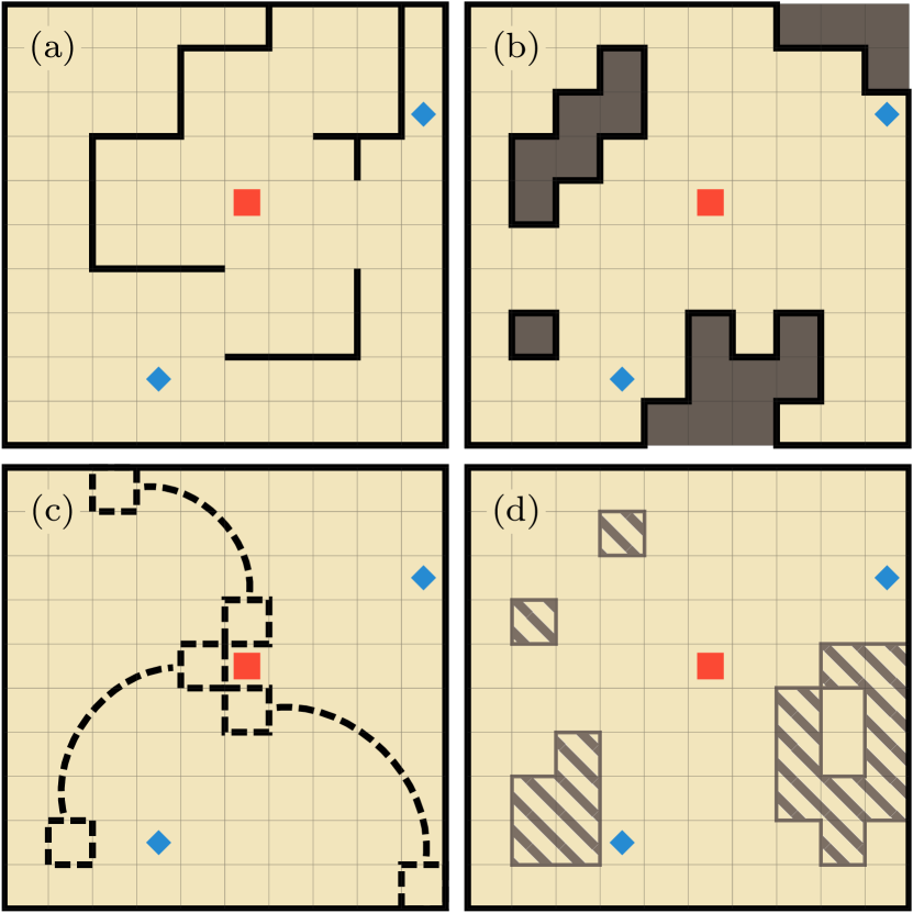
Figure 1: Examples of the spatial heterogeneities within a square lattice of width 10 with reflecting boundaries. Panel (a) represents an open partitions with the solid black lines indicating impenetrable barriers. When these barriers enclose a region, some space becomes inaccessible indicated by the sites coloured dark grey in panel (b). Panel (c) shows a lattice where three pairs of non-neighbouring sites have a long range connection, i.e. transitions from a dashed site include the nearest-neighbours as well as the site connected via the dashed line. Panel (d) is an example of where the diffusivity of the striped sites is smaller than the regular (non-striped) sites. The central site flagged by a red square and the two sites flagged by a blue diamond are, respectively, the initial condition and the absorbing targets for use in later sections.

The heterogeneities displayed in Fig. 1 emerge from the modification of the outgoing transitions from one or more sites, hence we refer to these altered transitions as heterogeneous connections. For example, given a partially reflecting barrier in between two neighbouring sites, the jump probability from either of the two sites to the other is reduced, while the probability of staying put at either of the sites is increased. Conversely, by connecting together two non-neighbouring sites, we may wish to reduce the probability of staying put at a given site, whilst adding the possibility of hopping to the site further away. One can represent conveniently these or any other heterogeneity through a modification of the transitions as depicted in Fig. 2. Formally, the outgoing connections of the sites $\bm{u}$ and $\bm{\varvb}$ are adjusted by introducing the parameters $\lambda_{{{\bm{\varvb}}},{{\bm{u}}}}$ and $\lambda_{{{\bm{u}}},{{\bm{\varvb}}}}$ to create two heterogeneous connections. Although we choose to modify transitions in both direction, i.e. from $\bm{u}$ to $\bm{\varvb}$ and $\bm{\varvb}$ to $\bm{u}$, this does not have to be the case. Modifications of only outgoing connections are also permitted, e.g. see the dashed arrows connecting the additional sites $\bm{r}$ and $\bm{s}$.

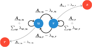
Figure 2: A schematic representation of the transition probabilities after the introduction of spatial heterogeneity or disorder. The probability of hopping from site $\bm{u}$ to $\bm{\varvb}$ is given by $\underline{\bm{A}}_{{\bm{\varvb}},{\bm{u}}}$. When $\lambda_{{{\bm{\varvb}}},{{\bm{u}}}}$ is positive, the probability of jumping from $\bm{u}$ to $\bm{\varvb}$ decreases, while the probability of staying put increases. When $\lambda_{{{\bm{\varvb}}},{{\bm{u}}}}$ is negative, the opposite effect occurs with a decrease in the probability of staying, while increasing the jump probability from $\bm{u}$ to $\bm{\varvb}$. The parameter $\lambda_{{{\bm{u}}},{{\bm{\varvb}}}}$ affects the transition probability from $\bm{\varvb}$ to $\bm{u}$ and the probability of remaining at $\bm{\varvb}$ in an equivalent manner.

The construction implicitly conserves probability, which can be evinced by picking a defect, e.g. $\bm{u}$, and summing over all of the outgoing probabilities. The changes induced by the $\lambda$ parameters cancel each other out leaving $\sum_{\bm{w}}\underline{\bm{A}}_{{\bm{w}},{\bm{u}}}$, with $\bm{w}$ representing all the neighbours of $\bm{u}$, equal to the homogeneous outgoing probability. To ensure positive probability for a given heterogeneous site $\bm{u}$, we have the conditions

$$\lambda_{{{\bm{w}}},{{\bm{u}}}}\leq\underline{\bm{A}}_{{\bm{w}},{\bm{u}}},$$ (2)

for all $\bm{w}$ with a heterogeneous connection in the direction $\bm{u}$ to $\bm{w}$, and

$$0\leq\underline{\bm{A}}_{{\bm{u}},{\bm{u}}}+\sum_{\bm{w}}\lambda_{{{\bm{w}}},{{\bm{u}}}},$$ (3)

which enforces upper and lower bounds on the $\lambda$ parameters although each one of them can be positive or negative. This formulation allows one to perturb arbitrarily the homogeneous lattice creating any type of probability conserving particle-environment interactions.

II.1 Quantitative representation of heterogeneities

To understand the practicality of the formalism, we focus on the three specific types of heterogeneities in Fig. 1, namely, barriers (Figs. (1)a and (1)b), long-range connections (Fig. 1c) and sticky sites (Fig. 1d). In the following subsection we present convenient parameterisation for the constant $\lambda$’s to construct such heterogeneities.

II.1.1 Barriers and Anti-Barriers

With $\bm{u}$ and $\bm{\varvb}$ two neighbouring sites, we construct a partially reflecting barrier by having $\lambda_{{{\bm{\varvb}}},{{\bm{u}}}}=\alpha_{\bm{\varvb}}\underline{\bm{A}}_{{\bm{\varvb}},{\bm{u}}}$ and $\lambda_{{{\bm{u}}},{{\bm{\varvb}}}}=\alpha_{\bm{u}}\underline{\bm{A}}_{{\bm{u}},{\bm{\varvb}}}$ where $\alpha_{\bm{\varvb}},\alpha_{\bm{u}}\in[0,1]$ is a measure of the reflectivity of the barrier. When $\alpha_{\bm{\varvb}},\alpha_{\bm{u}}=1$ we have an impenetrable barrier (shown in Fig. 3), while with $\alpha_{\bm{\varvb}},\alpha_{\bm{u}}=0$ we regain the homogeneous transition. Notice that the barrier does not need to be symmetric, i.e. $\alpha_{\bm{u}}\neq\alpha_{\bm{\varvb}}$, with the extreme scenario being a barrier with $\lambda_{{{\bm{\varvb}}},{{\bm{u}}}}=\underline{\bm{A}}_{{\bm{\varvb}},{\bm{u}}}$ and $\lambda_{{{\bm{u}}},{{\bm{\varvb}}}}=0$ yields a one-way barrier or gate. In such a case the movement from $\bm{\varvb}$ to $\bm{u}$ is allowed but from $\bm{u}$ to $\bm{\varvb}$ is not.

It is also possible to have dynamics opposite to the partially reflecting barrier. In this case, again with $\bm{u}$ and $\bm{\varvb}$ two neighbouring sites, one has $\lambda_{{{\bm{\varvb}}},{{\bm{u}}}}=-\beta_{\bm{\varvb}}\underline{\bm{A}}_{{\bm{u}},{\bm{u}}}$ and $\lambda_{{{\bm{u}}},{{\bm{\varvb}}}}=-\beta_{\bm{u}}\underline{\bm{A}}_{{\bm{\varvb}},{\bm{\varvb}}}$ where $\beta_{\bm{\varvb}},\beta_{\bm{u}}\in[0,1]$. As the probability of jumping to the neighbours increases whilst the probability of staying put decreases, we have chosen the name anti-barrier for this type of heterogeneity.

Figure 3: Example of a reflecting barrier between $\bm{u}$ and $\bm{\varvb}$ generated by modifying the transition probabilities (from the left to the right of the schematic). The modified transitions are indicated by coloured arrows. The modification in this case results in an impenetrable barrier between $\bm{u}$ and $\bm{\varvb}$, with $\alpha_{\bm{\varvb}}=\alpha_{\bm{u}}=1$.

II.1.2 Long Range Connection

When adding an outgoing long-range connection one has to draw the probability from one or more of the existing transitions. Let us consider a site $\bm{u}$ and a non-neighbouring destination site $\bm{s}$, where $\underline{\bm{A}}_{{\bm{s}},{\bm{u}}}=\underline{\bm{A}}_{{\bm{u}},{\bm{s}}}=0$. One way of introducing the outgoing long range connection is to draw upon the lazy (also called sojourn) probability using $\lambda_{\bm{s},\bm{u}}=-\beta_{\bm{s}}\underline{\bm{A}}_{{\bm{u}},{\bm{u}}}$ and $\lambda_{\bm{u},\bm{s}}=-\beta_{\bm{u}}\underline{\bm{A}}_{{\bm{s}},{\bm{s}}}$, where $\beta_{\bm{u}},\beta_{\bm{s}}\in[0,1]$ is the proportion of the lazy probability added to the long range connection, see Fig. 4 for a pictorial representation.

Note this is not the only way; one can also rewire an existing connection from a neighbour to the non-neighbour. In such a case, with $\bm{\varvb}$ a neighbour of $\bm{u}$, we let $\lambda_{{{\bm{\varvb}}},{{\bm{u}}}}=\underline{\bm{A}}_{{\bm{\varvb}},{\bm{u}}}$ and $\lambda_{{{\bm{s}}},{{\bm{u}}}}=-\underline{\bm{A}}_{{\bm{\varvb}},{\bm{u}}}$. The former removes the possibility of jumping from $\bm{u}$ to the neighbour $\bm{\varvb}$, whilst the latter adds the possibility of hopping from $\bm{u}$ to the non-neighbour $\bm{s}$.

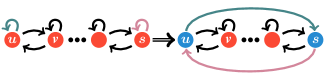
Figure 4: Example of a long range connection obtained by rewiring the lazy probability of $\bm{u}$ and $\bm{\varvb}$ to create a long range connection between them (from left to right). In this case $\beta_{\bm{u}}=\beta_{\bm{s}}=1$.

II.1.3 Sticky and Slippery Sites

Adding a partially reflecting barrier between two neighbouring sites naturally increases the probability of staying. By harnessing this property one can use multiple one-way partially reflecting barriers between a site $\bm{w}$ and all of its $k$ nearest neighbours, $\bm{r}_{1},\cdots,\bm{r}_{k}$, giving $\lambda_{{{\bm{r}_{i}}},{{\bm{w}}}}=\alpha\underline{\bm{A}}_{{\bm{r}_{i}},{\bm{w}}}$, and $\lambda_{{{\bm{w}}},{{\bm{r}_{i}}}}=0$ with $\alpha\in[0,1]$ for all $i=1,\cdots,k$. The result is a sticky site, $\bm{w}$, where the probability of staying is increased, whilst the probability of jumping to any of its neighbours is decreased. The introduction of $\alpha$ is used to control and distribute the stickiness equally across the neighbours in a convenient manner. See Fig. 5 for a pictorial representation on a 1D lattice.

Conversely, keeping $\lambda_{{{\bm{w}}},{{\bm{r}_{i}}}}=0$ and letting $\lambda_{{{\bm{r}_{i}}},{{\bm{w}}}}=-\frac{\beta}{k}\underline{\bm{A}}_{{\bm{w}},{\bm{w}}}$ with $\beta\in[0,1]$ for all $i=1,\cdots,k$ yields a slippery site with opposite dynamics. As for the sticky site, the introduction of $\beta$ is used to control the slippery quality of the site $\bm{w}$ equally among its neighbours. Note that we have chosen to divide $\beta$ by $k$ so that Eq. 3 is automatically satisfied.

Figure 5: Example of a sticky site on a 1D lattice generated by reducing all of the outgoing probability to the neighbours as shown by the thinner arrows, whilst increasing the staying probability of $\bm{w}$ as shown by the thicker self loop (from left to right).

III Heterogeneous Propagator

We consider an arbitrary collection of heterogeneous connections given by a set of $M$ paired defective sites or defects, $S=\left\{\{\bm{u}_{1},\bm{\varvb}_{1}\},\cdots,\{\bm{u}_{M},\bm{\varvb}_{M}\}\right\}$. We use $\bm{u}_{i}$ and $\bm{\varvb}_{i}$ with subscripts to indicate the two members of the $i^{\mathrm{th}}$ pair, while $\bm{u}$ and $\bm{\varvb}$ without subscripts refers to a generic pair in $S$. The pairs are unique, i.e. $\left\{\bm{u}_{i},\bm{\varvb}_{i}\right\}\neq\left\{\bm{u}_{j},\bm{\varvb}_{j}\right\}$ for any $i\neq j$, however, a site can be part of multiple pairs. For example, the set of pairs which represents the schematic depicted in Fig. 2 is $S=\left\{\{\bm{u},\bm{\varvb}\},\{\bm{u},\bm{r}\},\{\bm{\varvb},\bm{s}\}\right\}$, with the sites $\bm{u}$ and $\bm{\varvb}$ being part of two pairs while the sites $\bm{r}$ and $\bm{s}$ being part of only one pair each. The evolution of the occupation probability is given by the Master equation (for the details see LABEL:sup-sec:refl_defect_deriv of the Supplementary Materials)

$$\begin{split}&\Phi(\bm{n},t+1)=\sum_{\bm{m}}\underline{\bm{A}}_{\bm{n},\bm{m}}\,\Phi(\bm{m},t)\\ &+\sum_{k=1}^{M}\left(\delta_{\bm{n},\bm{u}_{k}}-\delta_{\bm{n},\bm{\varvb}_{k}}\right)\left[\bigg{.}\lambda_{{{\bm{\varvb}}}_{{k}},{{\bm{u}}}_{{k}}}\Phi(\bm{u}_{k},t)-\lambda_{{{\bm{u}}}_{{k}},{{\bm{\varvb}}}_{{k}}}\Phi(\bm{\varvb}_{k},t)\right],\end{split}$$ (4)

where the second summation is over all pairs of heterogeneous connections. When all $\lambda$ parameters are set equal to zero, Eq. 4 reduces to Eq. 1 and the occupation probability on the heterogeneous lattice, $\Phi{(\bm{n},t)}$, reduces to that of the homogeneous lattice, $\varphi{(\bm{n},t)}$.

One can find the generating function ($z$-domain) solution of Eq. 4 by generalising the so-called defect technique to obtain (see LABEL:sup-sec:refl_defect_deriv of the Supplementary Materials)

$$\widetilde{\Phi}_{{\bm{n}_{0}}}{({\bm{n}},z)}=\widetilde{\varphi}_{{\bm{n}_{0}}}{({\bm{n}},z)}-1+\frac{\left|\underline{\bm{H}}{\left({\bm{n}},{\bm{n}_{{0}}}\right)}\right|}{\left|\underline{\bm{H}}\right|},$$ (5)

where $\widetilde{f}(z)=\sum_{t=0}^{\infty}f(t)z^{t}$ is the generating function of the time dependent function $f(t)$, $\widetilde{\varphi}_{{\bm{n}_{0}}}{({\bm{n}},z)}$ is the propagator generating function of Eq. 1, while $\left|\underline{\bm{H}}\right|$ and $\left|\underline{\bm{H}}{\left({\bm{n}},{\bm{n}_{{0}}}\right)}\right|$ are determinants with

$$\underline{\bm{H}}_{{{i},{j}}}=\lambda_{{{\bm{\varvb}}}_{{i}},{{\bm{u}}}_{{i}}}\widetilde{\varphi}_{\left\langle\bm{u}_{j}-\bm{\varvb}_{j}\right\rangle}{({\bm{u}_{i}},z)}-\lambda_{{{\bm{u}}}_{{i}},{{\bm{\varvb}}}_{{i}}}\widetilde{\varphi}_{\left\langle\bm{u}_{j}-\bm{\varvb}_{j}\right\rangle}{({\bm{\varvb}_{i}},z)}$$

$$\phantom{\underline{\bm{H}}_{{{i},{j}}}}-z^{-1}\delta_{i,j},$$ (6)

$$\underline{\bm{H}}{\left({\bm{n}},{\bm{n}_{{0}}}\right)}_{{{i},{j}}}=\underline{\bm{H}}_{{{i},{j}}}-\widetilde{\varphi}_{\left\langle\bm{u}_{j}-\bm{\varvb}_{j}\right\rangle}{({\bm{n}},z)}$$

$$\phantom{\underline{\bm{H}}{\left({\bm{n}},{\bm{n}_{{0}}}\right)}_{{{i},{j}}}}\times\left[\lambda_{{{\bm{\varvb}}}_{{i}},{{\bm{u}}}_{{i}}}\widetilde{\varphi}_{{\bm{n}_{0}}}{({\bm{u}_{i}},z)}-\lambda_{{{\bm{u}}}_{{i}},{{\bm{\varvb}}}_{{i}}}\widetilde{\varphi}_{{\bm{n}_{0}}}{({\bm{\varvb}_{i}},z)}\right].$$ (7)

In Sections III and III we have used the notation $\widetilde{\varphi}_{\left\langle\bm{u}-\bm{\varvb}\right\rangle}{({\bm{n}},z)}=\widetilde{\varphi}_{{\bm{u}}}{({\bm{n}},z)}-\widetilde{\varphi}_{{\bm{\varvb}}}{({\bm{n}},z)}$. From here onwards we refer to $\widetilde{\varphi}_{{\bm{n}_{0}}}{({\bm{n}},z)}$ as the homogeneous propagator, which is known explicitly (see LABEL:sup-sec:block_matrix_const and LABEL:sup-sec:eigvecs_eigvals_props of the Supplementary Materials), while $\widetilde{\Phi}_{{\bm{n}_{0}}}{({\bm{n}},z)}$ is referred to as the heterogeneous propagator. When $t=0$, that is $z=0$, we have $\widetilde{\varphi}_{\bm{n}_{0}}{\left(\bm{n},0\right)}=\delta_{\bm{n}_{0},\bm{n}}$, while $\left|\underline{\bm{H}}{\left({\bm{n}},{\bm{n}_{{0}}}\right)}\right|/\left|\underline{\bm{H}}\right|=1$ and we recover the appropriate initial condition, $\widetilde{\Phi}_{\bm{n}_{0}}{\left(\bm{n},0\right)}=\delta_{\bm{n}_{0},\bm{n}}$.

In general the size of matricies $\underline{\bm{H}}$ and $\underline{\bm{H}}{\left({\bm{n}},{\bm{n}_{{0}}}\right)}$ depends on the number of paired defects, $M$. A $d$-dimensional walk with one sticky (or slippery) site requires two paired defects for each of the $d$ dimensions. However, in this case one can make a simplification and reduce the size of the matrices by a factor of $2d$. The simplified matrices $\underline{\bm{H}}$ and $\underline{\bm{H}}{\left({\bm{n}},{\bm{n}_{{0}}}\right)}$ are defined, respectively, in LABEL:sup-eq:hmat_sticky and LABEL:sup-eq:hcn0mat_sticky of the Supplementary Materials.

In Fig. 6 we plot a snapshot of $\widetilde{\Phi}_{\bm{n}_{0}}(\bm{n},t)$ for the heterogeneities depicted in each of the panels of Fig. 1.

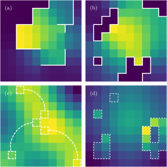
Figure 6: A snapshot of $\Phi_{{\bm{n}_{0}}}{({\bm{n}},{t})}$ at time $t=100$ obtained from Eq. 5 with standard numerical methods [59, 60]. Propagator with different configurations of defects, corresponding with Fig. 1, at $t=100$. For all panels, the homogeneous propagator, $\widetilde{\varphi}_{{\bm{n}_{0}}}{({\bm{n}},z)}$ is the 2D propagator with reflecting boundaries given in Eq. (23) of Ref. [58] (see also LABEL:sup-sec:eigvecs_eigvals_props of the Supplementary Materials). The parameters used are: a domain of size $\bm{N}=(10,10)$, a localised initial condition with $\bm{n}_{0}=(6,6)$. We a use diffusion parameter of value $\bm{q}=(0.2,0.2)$, which gives the following transition probabilities: in the bulk of the homogeneous lattice the probability of jumping to one of the four neighbours is $\underline{\bm{A}}_{{\bm{r}},{\bm{s}}}=0.05$ (with $\bm{r}\neq\bm{s}$), while the probability of staying at the same site is $\underline{\bm{A}}_{{\bm{r}},{\bm{r}}}=0.8$. The reflecting barriers and other heterogeneities are super imposed on top of the probability. For panels (a) and (b), $\lambda_{{{\bm{\varvb}}},{{\bm{u}}}}=\underline{\bm{A}}_{{\bm{\varvb}},{\bm{u}}}$ and $\lambda_{{{\bm{u}}},{{\bm{\varvb}}}}=\underline{\bm{A}}_{{\bm{\varvb}},{\bm{u}}}$ (for all $\left\{\bm{u},\bm{\varvb}\right\}\in S$) yielding perfectly reflecting barriers. For panel (c) $\lambda_{{{\bm{\varvb}}},{{\bm{u}}}}=-\frac{1}{2}\underline{\bm{A}}_{{\bm{u}},{\bm{u}}}$, and $\lambda_{{{\bm{u}}},{{\bm{\varvb}}}}=-\frac{1}{2}\underline{\bm{A}}_{{\bm{\varvb}},{\bm{\varvb}}}$. With this perturbation, when on one of the defective sites, the probability of staying is reduced to $\underline{\bm{A}}_{{\bm{u}},{\bm{u}}}=\underline{\bm{A}}_{{\bm{\varvb}},{\bm{\varvb}}}=0.4$, while the probability of jumping to the non-neighbour is increased (from zero) to $\underline{\bm{A}}_{{\bm{u}},{\bm{\varvb}}}=\underline{\bm{A}}_{{\bm{\varvb}},{\bm{u}}}=0.4$. Lastly, for panel (d), for each of the sticky-sites $\bm{w}$ with $k$ neighbours $\bm{r}_{1},\cdots,\bm{r}_{k}$ we use $\lambda_{{{\bm{r}_{i}}},{{\bm{w}}}}=\frac{1}{4}\underline{\bm{A}}_{{\bm{r}_{i}},{\bm{w}}}$ (see Section II.1.3). For convenience we have omitted colour bars for each panel as we are interested only in the relative differences of the occupation probability.

In panel (a) the lattice is partitioned by impenetrable barriers represented by the solid white lines. Here, one can observe the lowest probabilities in the top-left corner since the walker has not had the time to travel around the barriers. Panel (b) contains areas enclosed by impenetrable barriers, with occupation probabilities that are always zero. The long range connection shown in panel (c) has enabled the walker to spread further than in other panels. Small peaks in the probability can be observed away from the initial condition, in the top-left, bottom-left and bottom right corners. In panel (d) the sticky regions tend to show a higher occupation probability compared to the homogeneous sites.

Figure 7: Time-dependent first-passage probability to either of two targets in the presence of heterogeneities. The location of the targets $\bm{n}_{1}=(4,2)$ and $\bm{n}_{2}=(10,7)$ in relation to the initial condition $\bm{n}_{0}=(6,6)$ and visualisation of the heterogeneities present can be seen in the schematic diagram in Fig. 1. We use a homogeneous propagator, $\widetilde{\varphi}_{{\bm{n}_{0}}}{({\bm{n}},z)}$ with a reflecting domain of size $\bm{N}=(10,10)$ and a diffusion parameter of value $\bm{q}=(0.2,0.2)$. The explicit form of $\widetilde{\varphi}_{{\bm{n}_{0}}}{({\bm{n}},z)}$ is given by Eq. (23) of Ref. [58]. The lines are obtained through numerical inversion of the generating function of the first-passage probability to either of two targets (see text), while the corresponding marks—shown only in panel (a)—are obtained through $1.5\times 10^{6}$ stochastic simulations.

Note that we have not placed any restriction on whether (the homogeneous propagator) $\widetilde{\varphi}_{{\bm{n}_{0}}}{({\bm{n}},z)}$ conserves probability or note. When there are fully or partially absorbing sites, one may proceed in two ways. (i) In the first approach one account for the absorbing dynamics by finding the propagator $\widetilde{\varphi}_{{\bm{n}_{0}}}{({\bm{n}},z)}$ that satisfies appropriate boundary conditions, before adding inert disorder via Eq. 5. (ii) In the second approach one would take $\widetilde{\varphi}_{{\bm{n}_{0}}}{({\bm{n}},z)}$ without any absorbing locations, construct $\widetilde{\Phi}_{{\bm{n}_{0}}}{({\bm{n}},z)}$ and then add the absorbing sites using the standard defect technique in the presence of absorbing sites [50]. While the choice makes no impact on the final dynamics, depending on the situation one procedure may be more convenient than the other.

IV First-Passage Processes

An important quantity derived from the propagators is the first-passage statistics to a set of targets. It is relevant to stochastic search in movement ecology [61], swarm robotics [62] and many other areas [63].

The first-passage probability, $\mathbb{F}_{{\bm{n}_{0}}}{({\bm{n}},{t})}$, that is the probability to reach $\bm{n}$ for the first time at $t$ having started at $\bm{n}_{0}$, is related to the propagator, $\Phi_{{\bm{n}_{0}}}{({\bm{n}},{t})}$ by the renewal equation. When $\bm{n}\neq\bm{n}_{0}$, the well-known relation in $z$-domain is given by $\widetilde{\mathbb{F}}_{{\bm{n}_{0}}}{({\bm{n}},z)}=\widetilde{\Phi}_{{\bm{n}_{0}}}{({\bm{n}},z)}/\widetilde{\Phi}_{{\bm{n}}}{({\bm{n}},z)}$. Having the first-passage probability in closed form allows one to substitute the heterogeneous first-passage probability $\mathbb{F}_{{n_{0}}}{({n},{t})}$ (or $\widetilde{\mathbb{F}}_{{n_{0}}}{({n},z)}$) in place of the homogeneous counterpart in other established contexts where homogeneous space was previously assumed.

One such context is a first-passage in the presence of multiple targets, where one is interested in the probability of being absorbed at any of the targets. We use recent findings [58] to determine the dynamics of a lattice walker to reach either of two sites, $\bm{n}_{1}$, and $\bm{n}_{2}$, for the first time at $t$ in the presence of spatial heterogeneities, given by $\mathbb{F}_{{\bm{n}_{0}}}{({\bm{n}_{1},\bm{n}_{2}},{t})}$. The generating function of this probability, given by $\widetilde{\mathbb{F}}_{{\bm{n}_{0}}}{({\bm{n}_{1},\bm{n}_{2}},z)}=\left\{\widetilde{\mathbb{F}}_{{\bm{n}_{0}}}{({\bm{n}_{1}},z)}\left[-\widetilde{\mathbb{F}}_{{\bm{n}_{1}}}{({\bm{n}_{2}},z)}\right]+\widetilde{\mathbb{F}}_{{\bm{n}_{0}}}{({\bm{n}_{2}},z)}\left[-\widetilde{\mathbb{F}}_{{\bm{n}_{2}}}{({\bm{n}_{1}},z)}\right]\right\}\\ \times\left[1-\widetilde{\mathbb{F}}_{{\bm{n}_{1}}}{({\bm{n}_{2}},z)}\widetilde{\mathbb{F}}_{{\bm{n}_{1}}}{({\bm{n}_{2}},z)}\right]^{-1}$, (taken from Eq. (38) in Ref. [58]), is expressed in terms of the first-passage probabilities to single targets.

In Fig. 7 plot the time dependent probability for the heterogeneity examples shown in Fig. 1. The first non-zero probability corresponds to the length of the shortest path to either of the targets, which in the absence of heterogeneities and for the examples in Fig. 1(a), (b) and (d) is 6, whereas for the panel (c) one can reach the target $\bm{n}_{1}$ from $\bm{n}_{0}$ in 4 steps as a result of the nearest long range connection. It is clearly visible in the earlier rise of the curve related to Fig. 1(c). Interestingly, the first-passage probability curves corresponding with excluded regions, shown in Fig. 1(b), and the homogeneous case are almost indistinguishable from each other for 2 decades. While excluding parts of the lattice increases the lengths of some paths to the targets, it also reduces the overall space that can be explored. For the setup chosen, these two effects counteract each other at short and intermediate timescales.

Among all the curves, the case with open partitions related to Fig. 1(a), results in a first-passage probability which is the slowest to rise and with the broadest tail in the distribution. The reasons for such characteristics compared to all other curves is due to the location of the initial site relative to the targets. As the latter ones are partially behind partitions, the more directed paths take more time to reach the targets and the walker remains confined in the region around the initial site for much longer.

The sticky sites in Fig. 1(d) have limited effect on the more directed paths connecting the starting site and the targets. This is why $\mathbb{F}_{{\bm{n}_{0}}}{({\bm{n}_{1},\bm{n}_{2}},{t})}$ in Fig. 7(b) is identical to the homogeneous case at short times. However, sticky-sites can be both a hindrance or a benefit to the searcher. While it can partially trap the walker and stop it from reaching the target site, it can also stop the walker from exploring regions away from the targets. Since there are sticky sites close to the targets, these two effects counteract one another and we observe marginal difference in the tail of the distribution when compared with the homogeneous curve.

IV.1 Explicit mean first-passage quantities

The first moment of $\mathbb{F}_{{\bm{n}_{0}}}{({\bm{n}},{t})}$, that is the mean first-passage time (MFPT), $\mathfrak{F}_{{\bm{n}_{0}}\to{\bm{n}}}=\left.\frac{\mathrm{d}}{\mathrm{d}z}\widetilde{\mathbb{F}}_{{\bm{n}_{0}}}{({\bm{n}},z)}\right|_{z=1}$, is given by

$$\mathfrak{F}_{{\bm{n}_{0}}\to{\bm{n}}}=\frac{\mathcal{F}_{{\bm{n}_{0}}\to{\bm{n}}}\left|\underline{\bm{\mathcal{H}}}-1/\mathcal{F}_{{\bm{n}_{0}}\to{\bm{n}}}\underline{\bm{\mathcal{H}}}^{{({1})}}\right|}{\left|\underline{\bm{\mathcal{H}}}-\underline{\bm{\mathcal{H}}}^{{({2})}}\right|},$$ (8)

where $\mathcal{F}_{{\bm{n}_{0}}\to{\bm{n}}}$ is the homogeneous MFPT from $\bm{n}_{0}$ to $\bm{n}$ and the elements of the matrices $\underline{\bm{\mathcal{H}}}$, $\underline{\bm{\mathcal{H}}}^{{({1})}}$ and $\underline{\bm{\mathcal{H}}}^{{({2})}}$ are defined in terms of homogeneous MFPTs. They are given, respectively, in Eqs. 16, 17 and 18 for general heterogeneities, while for the case with only sticky or slippery heterogeneities the matrices are given by LABEL:sup-eq:mean_hij_1_sticky, LABEL:sup-eq:mean_h1ij_1_sticky and LABEL:sup-eq:mean_h2ij_1_sticky in the Supplementary Materials. In the coming sections we use the mathfrak notation e.g. $\mathfrak{F},\mathfrak{R}$ and $\mathfrak{E}$, for statistics involving the heterogeneous dynamics, while the mathcal notation, e.g. $\mathcal{F},\mathcal{R}$ and $\mathcal{E}$, is reserved for the homogeneous counterpart. The dependence on the target at $\bm{n}$ is only present in the matrices $\underline{\bm{\mathcal{H}}}^{{({1})}}$ and $\underline{\bm{\mathcal{H}}}^{{({2})}}$; the dependence on the initial condition $\bm{n}_{0}$ is only present in $\underline{\bm{\mathcal{H}}}^{{({1})}}$; and the dependence on the location of the heterogeneities are in all three matrices.

The probability distribution of the first-return time is related to the propagator via $\widetilde{\mathbb{R}}{({\bm{n}},z)}=1-\widetilde{\Phi}^{-1}_{{\bm{n}}}{({\bm{n}},z)}$, with a mean return time (MRT) given by

$$\mathfrak{R}_{\bm{n}}=\frac{\mathcal{R}_{\bm{n}}\left|\underline{\bm{\mathcal{H}}}\right|}{\left|\underline{\bm{\mathcal{H}}}-\underline{\bm{\mathcal{H}}}^{{({2})}}\right|},$$ (9)

where $\mathcal{R}_{\bm{n}}$ is the homogeneous mean return time.

When the heterogeneities preserve the symmetric properties of the homogeneous lattice, i.e. the disorder does not add any bias to a diffusive system or remove any bias present in a system with drift, then the ratio $\small{\underline{\bm{A}}_{{\bm{u}},{\bm{\varvb}}}}/{\underline{\bm{A}}_{{\bm{\varvb}},{\bm{u}}}}={\left(\underline{\bm{A}}_{{\bm{u}},{\bm{\varvb}}}-\lambda_{{{\bm{u}}},{{\bm{\varvb}}}}\right)}/{\left(\underline{\bm{A}}_{{\bm{\varvb}},{\bm{u}}}-\lambda_{{{\bm{\varvb}}},{{\bm{u}}}}\right)}$ is satisfied, for all $\{\bm{u},\bm{\varvb}\}\in S$, and the heterogeneous system maintains the steady state of the homogeneous system. In this case, $\underline{\bm{\mathcal{H}}}^{{({2})}}=0$, the MFPT given by Eq. 8, can be simplified to $\mathfrak{F}_{{\bm{n}_{0}}\to{\bm{n}}}=\mathcal{F}_{{\bm{n}_{0}}\to{\bm{n}}}-1+\left|\underline{\bm{\mathcal{H}}}-\underline{\bm{\mathcal{H}}}^{{({1})}}\right|/\left|\underline{\bm{\mathcal{H}}}\right|$, while the MRT remains the same as the homogeneous MRT, $\mathfrak{R}_{\bm{n}}=\mathcal{R}_{\bm{n}}$ as expected from Kac’s lemma [64]. (see Section A.1 and LABEL:sup-sec:mret_deriv of the Supplementary Materials).

In the presence of multiple targets at the outer boundary of the domain, we relate the first-passage probability to any of the targets to a propagator with the appropriate absorbing boundaries. In this case, the first-passage is referred to as the first-exit, and its probability generating function is related to the propagator through the relation $\widetilde{\mathbb{E}}_{{\bm{n}_{0}}}{(z)}=1-(1-z)\widetilde{\mathbb{S}}_{{\bm{n}_{0}}}{(z)}$, where $\widetilde{\mathbb{S}}_{{\bm{n}_{0}}}{(z)}$ is the survival probability. Taking the mean of the distribution (see Section A.2) gives

$$\mathfrak{E}_{{\bm{n}_{0}}}=\widetilde{\mathbb{S}}_{\bm{n}_{0}}(z=1)=\left.\frac{\mathcal{E}_{{\bm{n}_{0}}}\left|\underline{\bm{H}}-1/\mathcal{E}_{{\bm{n}_{0}}}\underline{\bm{S}}{\left({\bm{n}_{{0}}}\right)}\right|}{\left|\underline{\bm{H}}\right|}\right|_{z=1}$$ (10)

where $\mathcal{E}_{{\bm{n}_{0}}}$ is the mean exit time starting at $\bm{n}_{0}$ without any heterogeneities, and the matrix $\underline{\bm{S}}{\left({\bm{n}_{{0}}}\right)}$ is given explicitly in Eq. 24. The presence of one or more absorbing boundaries on the homogeneous propagator $\widetilde{\varphi}_{{\bm{r}}}{({\bm{s}},z)}$ allows for a simple evaluation at $z=1$. That is to say $\widetilde{\varphi}_{\bm{r}}{(\bm{s},z=1)}$ is finite for any $\bm{r}$ and $\bm{s}$ in the domain; and therefore $\underline{\bm{H}}$ and $\underline{\bm{S}}{\left({\bm{n}_{{0}}}\right)}$ also remains finite and can be easily evaluated.

In Fig. 8 we show the effect of randomly distributed barriers and anti-barriers as a function of the barrier strength in a 2D domain with absorbing boundaries. The $M$ neighbouring defective site pairs are uniformly distributed on the lattice with $\lambda=\lambda_{{{\bm{\varvb}}},{{\bm{u}}}}=\lambda_{{{\bm{u}}},{{\bm{\varvb}}}}$ for all $\left\{\bm{u},\bm{\varvb}\right\}\in S$.

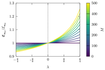
Figure 8: The ratio of the heterogeneous mean exit time $\mathfrak{E}_{{\bm{n}_{0}}}$ to the homogeneous mean exit time $\mathcal{E}_{{\bm{n}_{0}}}$ for randomly distributed barriers and anti-barriers. We use a homogeneous propagator with a domain of size $\bm{N}=(51,51)$ with absorbing boundary conditions, an initial condition at the centre of the domain $\bm{n}_{0}=(26,26)$ and a diffusion parameter of $\bm{q}=(0.8,0.8)$. The explicit form of $\widetilde{\varphi}_{{\bm{n}_{0}}}{({\bm{n}},z)}$ is given by the $z$-transform of Eq. (23) of Ref. [58]. Each curve is obtained using Eq. 10 and performing an ensemble average with $10^{2}$ sample realisations of locations of barriers ($\lambda>0$) or anti-barriers ($\lambda>0$) for each $\lambda$.

One can see that for $\lambda>0$, $\mathfrak{E}_{{\bm{n}_{0}}}$ increases, as the heterogeneous connections behave as a partially reflecting barrier slowing down the walker. Furthermore an increase in the number of heterogeneities resulting in larger exit times. Conversely, when $\lambda<0$ the heterogeneous connections become anti-barriers increasing the probability of jumping across compared to the homogeneous case, which effectively increases the spread of the walker leading to shorter exit times. When the barriers are impenetrable, increasing the number of barriers also increases the likelihood of the walker being trapped and unable to reach the boundary and will cause the MET to diverge. Although we do not study it here, a similar setup could be used to analyse percolation in finite multidimensional domains.

IV.2 First-passage processes in 1D with a single barrier and the phenomenon of disorder indifference of the MFPT

We consider a simple spatial heterogeneity in a 1D domain with a partially reflecting barrier between $u$ and $u+1$. To study the dependence of the position and strength of the barrier (or anti-barrier) on the first-passage dynamics, we first fix the position of target and initial sites with $n>n_{0}$; assume a reflecting boundary between $n=0$ and $n=1$; and take $\lambda_{u,u+1}=\lambda_{u+1,u}=\lambda$ with $\lambda\in[-(1-q),q/2]$. In this case the first passage probability can be written using the convenient notation

$$\widetilde{\mathbb{F}}_{{n_{0}}}{({n},z)}=\left\{\begin{array}[]{ll}\frac{a{\left(n_{0},z\right)}-\frac{2\lambda}{q}b{\left(n_{0},u,z\right)}}{a{\left(n,z\right)}-\frac{2\lambda}{q}b{\left(n,u,z\right)}}&u<n_{0}\\ &\\ \frac{a{\left(n_{0},z\right)}-\frac{2\lambda}{q}a{\left(n_{0},z\right)}}{a{\left(n,z\right)}-\frac{2\lambda}{q}b{\left(n,u,z\right)}}&u\geq n_{0}\end{array}\right.,$$ (11)

where $a(n,z)=\cosh{\left[\left(\frac{1}{2}-n\right)\zeta\right]}\cosh{\left[\frac{1}{2}\zeta\right]}$, $b(n,u,z)=\cosh{\left[\left(1-n\right)\zeta\right]}+\sinh{\left[\left(n-2u-\frac{1}{2}\right)\zeta\right]}\sinh{\left[\frac{1}{2}\zeta\right]}$, $\zeta=\mathrm{acosh}{\left[1-\frac{1}{q}\left(1-\frac{1}{z}\right)\right]}$, and with the probability of moving given by $q\in(0,1]$. The homogeneous first-passage probability, $\widetilde{F}_{{n_{0}}}{({n},z)}$, can be recovered from Eq. 11 by letting $\lambda\to 0$. When the barrier is to the left of the initial condition, the limit $\lambda\to\frac{q}{2}$ creates an impenetrable barrier, the behaviour is equivalent to shifting both the target and the initial condition to the left by $u$ giving $\widetilde{\mathbb{F}}_{{n_{0}}}{({n},z)}=\widetilde{F}_{{n_{0}-u}}{({n-u},z)}$. Whereas, when $n_{0}\leq u<n$, the same limit gives $\widetilde{\mathbb{F}}_{{n_{0}}}{({n},z)}=0$ as the walker becomes blocked by the barrier and can never reach the target.

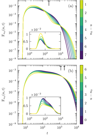
Figure 9: The time dependent first passage probability given through the numerical inversion of Eq. 11. Panel (a) represents the scenario $u<n_{0}<n$, while panel (b) is the case when $n_{0}\leq u<n$. The values of the other parameters are: $\lambda=0.975\cdot\frac{q}{2}$; a diffusion parameter of value $q=\frac{2}{3}$; the initial condition $n_{0}=8$; the target site $n=15$; and a reflecting boundary between $n=0$ and $n=1$. The arrows indicate the MFPTs: in panel (a) all of the curves have the same MFPT of $\mathfrak{F}_{{n_{0}}\to{n}}=231$ (disorder indifference), whereas in panel (b) the two arrows indicate the minimum and maximum MFPTs of the curves which are $\mathfrak{F}_{{n_{0}}\to{n}}=1167$ and $\mathfrak{F}_{{n_{0}}\to{n}}=1869$, and obtained, respectively, when $u=8$ and $u=14$

In Fig. 9, we plot the time dependence of Eq. 11 for the two different scenarios $u<n_{0}$ and $u\geq n_{0}$ represented, respectively, by panels (a) and (b). With $u<n_{0}$ and $\lambda<q/2$, that is the barrier to the left of the initial condition, as one increases $u$ from $u=1$ one observes an increase in the modal peak. When the walker is reflected by the permeable barrier, it stops the walker from straying further left and effectively reduces the space that can be explored, increasing the probability of reaching the target at an earlier time. However, if the walker passes through the barrier, the partial reflection dynamics becomes a hindrance: the walker is kept in the range $[1,u]$, causing the probability of reaching the target at long times to increase also. As probability in the tail and the mode increases, the probability conserving $\mathbb{F}_{{n_{0}}}{({n},{t})}$ demands a reduction at intermediate times, which is clearly visible from the figure. This permeability induced mode-tail enhancement can also be witnessed by fixing $u$ and changing $\lambda\in[0,q/2)$, and we have also observed the inverse effect, mode-tail compression by having anti-barrier with $\lambda\in[q-1,0]$. We have chosen not display these latter cases for want of space. Similar features have been observed in a diffusing diffusivity model in Ref. [35], where increases in the probability at short and long timescales were attributed to the dynamic diffusivity. Our findings point to the fact that such richness can also emerge from a static disorder at a single location.

Differently from the case when the barrier is to the left of the initial condition, is the case when $u\geq n_{0}$ . In this scenario, the barrier is always acting to slow the search process down, reducing the probability of reaching the target at early times and increasing the probability at long times as seen by the flattening of the mode and the broadening of the tail, as shown in Fig. 9(b).

Computing the mean via either Eq. 11 or from simplifying Eq. 8 yields the compact expression

$$\mathfrak{F}_{{n_{0}}\to{n}}=\mathcal{F}_{{n_{0}}\to{n}}+\frac{2}{q}\frac{\lambda}{\frac{q}{2}-\lambda}\left\{\begin{array}[]{ll}0,&u<n_{0},\\ u,&u\geq n_{0},\end{array}\right.$$ (12)

where $\mathcal{F}_{{n_{0}}\to{n}}=(n-n_{0})(n+n_{0}-1)/q$ is the 1D homogeneous MFPT for $n_{0}\leq n$ (given by Eq. (14) of Ref. [58]). Astonishingly, the mode-tail enhancement present in the time-dependent probability when $u<n_{0}$ has no effect on the mean. This is what we have termed the disorder indifference phenomenon.

To explain why there is such an effect of disorder indifference, we split the first passage trajectories into two mutually exclusive subsets: the trajectories that never return to the initial condition before reaching the target site on the right and those that return at least once before reaching the target site. Clearly, the former trajectories are unaffected by the presence of a barrier. The latter trajectories can be affected by the barrier, however, in computing the mean one deals with mean return times which are unaffected from the homogeneous case when $\lambda_{{{u}},{{u+1}}}=\lambda_{{{u+1}},{{u}}}$ as stated in the previous section (see Section B.1 for the mathematical details).

An analogue of this indifference phenomenon was observed in Ref. [40], where the MFPT in a quasi-1D domain in continuous space with two layers of different diffusivity was studied. When the initial condition was in between the interface of the layers and the target, they observed that the MFPT was indifferent to the diffusivity of the media beyond the interface. In that study, the first-passage probability was not considered and the cause of this indifference could not be quantified. However, one can relate the location of the interface of their system with the position of the barrier in ours. Through this relation, we believe that the behaviour observed in Ref. [40], is closely related to the dynamics presented in Fig. 9.

Given a barrier between the initial condition $n_{0}$ and the target $n$, the effect on the MFPT increases linearly as the displacement from the boundary increases. While the effect, which can be to speed up ($\lambda<0$) or to slow down ($\lambda>0$), is due to the disorder, the linear dependence is not. This linear dependence is present in all 1D situations and is proportional to the distance between the initial condition and the reflecting boundary (see Section B.2).

To explore the effects of asymmetry in the heterogeneities we consider the MRT with $\lambda_{{{u+1}},{{u}}}\neq\lambda_{{{u}},{{u+1}}}$. In this cases, the steady state is no longer homogeneous, effectively creating an out-of-equilibrium system due to the loss of detailed balance in the Master equation. To illustrate this point, we consider the MRT of a 1D walker within a segment of length $N$ with reflecting boundaries and with a barrier between $u$ and $u+1$, ($\lambda_{{{u+1}},{{u}}}\neq\lambda_{{{u}},{{u+1}}}$). In this case, Eq. 9 simplifies to

$$\mathfrak{R}_{n}=\left\{\begin{array}[]{ll}N\left[\frac{{q}/{2}-\lambda_{{{u+1}},{{u}}}}{{q}/{2}-\lambda_{{{u}},{{u+1}}}}\right]-u\left[\frac{\lambda_{{{u}},{{u+1}}}-\lambda_{{{u+1}},{{u}}}}{{q}/{2}-\lambda_{{{u}},{{u+1}}}}\right],&n<u+1,\\ &\\ N-u\left[\frac{\lambda_{{{u}},{{u+1}}}-\lambda_{{{u+1}},{{u}}}}{{q}/{2}-\lambda_{{{u+1}},{{u}}}}\right],&n\geq u+1,\end{array}\right..$$ (13)

One can see that when $\lambda_{{{u+1}},{{u}}}=\lambda_{{{u}},{{u+1}}}$, the MRT reduces to $N$ regardless of whether $n\leq u$ or $n>u$. In the extreme case, where the barrier is impenetrable in both direction, $\lambda_{{{u+1}},{{u}}}=\lambda_{{{u}},{{u+1}}}=q/2$, one can recover the appropriate MRTs when $n\leq u$ and $n>u$, which are, respectively, $u$ and $N-u$ (see LABEL:sup-sec:mret_limit of the Supplementary Materials).

Thus far we have focused on technical development and theoretical insights. As we move forward, the remainder of the article is devoted to practical examples, and is used to demonstrate the applicability of the framework. For practical convenience the details of the modelling set up are given in the appendices and only the results are discussed.

V Transdermal Drug Delivery

In the first application we consider the problem of optimising transdermal drug delivery, that is the transfer of drugs through the skin. One of the challenges of transdermal drug delivery is traversal of the outer-most layer of the epidermis called the stratum corneum (SC) by hydrophilic molecules [65]. This layer is made up of dead cells called corneocytes which are arranged in a dense ‘brick-and-mortar’ like pattern [66]. Inspired by some of the recent strategies proposed to enhance drug absorption [67], we consider the use of a micro-needles to pierce first the SC before applying a drug patch. We study the effectiveness of this method by using our modelling framework to represent the SC as heterogeneities on a lattice and modelling the movement of drug molecules as a random walk.

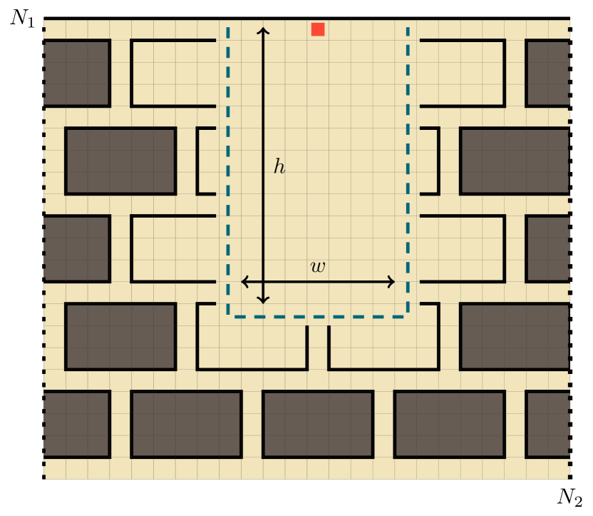
Figure 10: Representation of the ‘brick-and-mortar’ arrangement of the corneocytes in the stratum corneum (SC). The red square depicts the starting location of the random walker. The geometry is given by an an absorbing boundary at $n_{1}=1$, a reflecting boundary at $n_{2}=N_{1}$, shown as a thick solid black line, and a periodic boundary in the second dimension, depicted as dashed black lines. By using a number of paired defects, one is able to cordon off sites (shaded grey), creating the ‘brick-and-mortar’ pattern of the SC. The dashed blue rectangle with width $w$ and height $h$ models the destruction of the SC structure via a micro-needle puncture, with $h$ and $w$ representing, respectively, the puncture height and width. This destruction may open up some of the ‘bricks’, allowing the walker to easily travel inside. The initial position of the walker is at the centre-top of the puncture, $\bm{n}_{0}=(N_{1},N_{2}/2)$.

We use a homogeneous 2D nearest-neighbour random walker subject to mixed boundary conditions: an absorbing boundary located at $n_{1}=1$ and a reflecting boundary located at $n_{1}=N_{1}$, for the first dimension and a periodic boundary condition on the second dimension. The heterogeneities are impenetrable barriers representing the lipid matrix. These are arranged in a manner to create excluded regions that form the ‘brick-and-mortar pattern of the SC, see Fig. 10. The pattern is partially destroyed to represent the needle piercing in a rectangle with height $h$ and width $w$ resulting in an area absent of barriers as shown by the blue dashed rectangle in Fig. 10.

The quantity of interest is the MET with an initial condition starting at the reflecting end of the domain.

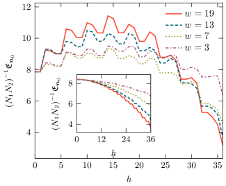
Figure 11: Mean exit time as a function of the puncture height, $h$, for different values of puncture width $w$ (see Fig. 10 for description of the setup). We use a rectangular domain of size $\bm{N}=(37,36)$, a diffusion parameter of $\bm{q}=(0.8,0.8)$, ‘bricks’ of size $(3,5)$ resulting in 9 layers with 6 bricks per layer, an initial condition of $\bm{n}_{0}=(1,19)$. The main panel depicts the scenario where the barriers encapsulating the ‘bricks’ are impenetrable, i.e. $\alpha_{\bm{\varvb}}=\alpha_{\bm{\varvb}}=1$ leading to $\lambda_{{{\bm{\varvb}}},{{\bm{u}}}}=\lambda_{{{\bm{u}}},{{\bm{\varvb}}}}=0.2$ for all $\bm{u},\bm{\varvb}$, while the inset shows the scenario where the barriers are partially permeable with $\alpha_{\bm{\varvb}}=\alpha_{\bm{\varvb}}=1$ giving $\lambda_{{{\bm{\varvb}}},{{\bm{u}}}}=\lambda_{{{\bm{u}}},{{\bm{\varvb}}}}=0.18$.

We plot the MET as a function of the puncture depth and width in Fig. 11. The overarching qualitative changes in the MET can be explained by two competing effects. The first is the breaking of enclosed bricks to create open partitions. The additional sites available for exploration makes the paths to reach the absorbing boundary longer.

The second effect is that the puncture allows the walker more direct movement towards the bottom layers leading to smaller MET. The removal of some of the impenetrable barriers allows for more direct paths to the absorbing boundary, which leads to smaller mean exit times. The strength of this effect is dependent on the size of the puncture $hw$. For small values of $h$, the first effect has greater influence leading to an increase in the METs. As $h$ is increased the second effect becomes more prominent and drives down the METs resulting in a global maximum. The interplay between the two effects also gives rise to the oscillations. Puncture of a brick layer opens it up, leading to larger exit times as the walker becomes temporarily confined inside a brick. Increasing the puncture height further destroys the brick structure of a layer and allows the walker to traverse the latter via a direct route thereby decreasing the exit times.

The global maximum and the oscillations are only present when the barriers are highly reflecting or impenetrable i.e. $0\ll\lambda_{{{\bm{\varvb}}},{{\bm{u}}}}\lambda_{{{\bm{u}}},{{\bm{\varvb}}}}\leq q/2$ for all $\left\{\bm{u},\bm{\varvb}\right\}\in S$. The maximum is lost when the permeability gets larger as the random walker is only partially confined by the barriers, leading to a monotonic decrease in the MET as seen in the inset of Fig. 11. With permeable barriers all the sites are always accessible independently of $h$ and $w$, puncturing only creates more direct routes to the absorbing boundary leading to smaller exit times.

VI Thigmotaxis

For the second application we look at thigmotaxis, which broadly speaking, is the movement of an organism due to a touch stimulus. We are interested specifically in the tendency of animals to remain close to the walls of an environment, a behaviour that is observed in many species from insects to mammals [68, 69].

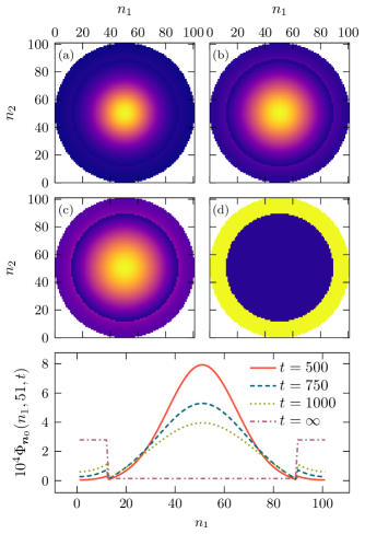
Figure 12: The propagator $\Phi_{{\bm{n}_{0}}}{({\bm{n}},{t})}$ at different moments in time, $t=500,750,1000,\infty$ where the walker is initially at the centre of the domain, $\bm{n}_{0}=(51,51)$. When inside the inner region the walker can freely enter the outer region without any resistance, that is $\lambda_{{{\bm{\varvb}}},{{\bm{u}}}}=0$ and when in the outer region the probability to move inward is modified via $\lambda_{{{\bm{u}}},{{\bm{\varvb}}}}=\alpha_{{i}}\underline{\bm{A}}_{{\bm{\varvb}},{\bm{u}}}$. Other parameters used are the diffusivity of value $\bm{q}=(0.8,0.8)$ and a square domain of size $\bm{N}=(101,101)$, (see Section C.1 for details on the placement of defects)

We quantify the thigomotactic tendency by appropriately selecting defects location and $\lambda$ to represent regions which are more easily accessible when moving in one direction (approaching boundaries) versus another (moving away from boundaries).

Since we are able to construct arbitrary shapes with the formalism, we consider two concentric circles within a square domain. The first is used to restrict the walker to a circular reflecting domain of radius $R$. The second has a radius $r$, with $r$ < $R$, and is used to partition the domain into two regions: an inner region; and an outer region, which is the annulus between $r$ and $R$, representing the preferred area of occupation. By placing one-way partially reflecting barriers along the radius $r$, we allow the walker to leave the inner region to enter the outer region without any resistance, while the tendency of remaining in the outer region is controlled by the parameter $\alpha_{i}\in[0,1]$. With $\alpha_{i}=1$ the walker never leaves the outer region once it gets there, whereas with $\alpha_{i}=0$, the partially reflecting barrier are removed and all areas of the circular domain becomes easily accessible. For a details on the placement of the defects and the construction of the circular domain see Section C.1.

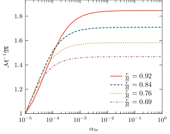
Figure 13: Saturated mean-squared displacement for a thigmotaxis process for different values of the ratios of $r/R$. We study the dynamics as a function of the normalised parameter $\alpha_{{i}}\in[0,1]$ which represents the tendency of the walker to remain close to the boundary. When $\alpha_{{i}}=0$, there are no outer or inner regions, while with $\alpha_{{i}}=1$, the walkers never leave the outer region once they they get there. The saturation MSD is normalised by $\mathcal{M}$, which is the saturation value when $\alpha_{{i}}=0$. Other parameters used are described in in the caption of Fig. 12.

Given these constraints we study the dynamics as a function of the $\alpha_{i}$. In Fig. 12, we plot the probability $\Phi_{{\bm{n}_{0}}}{({\bm{n}},{t})}$ for different values of $t=500,750,1000$ and $\infty$. The walker is initially at the centre of the domain $\bm{n}_{0}=(51,51)$ and can freely move inside the inner-region and is able to enter into the outer region without any resistance. However, once inside the outer region there is a greater tendency not to leave, due to the high value of $\alpha_{{i}}=0.95$. We observe this effect when going from panel (a) to (d). Initially the separation between the inner and outer regions are barely visible but as time progresses this separation becomes increasingly clear, culminating with a sharp step at the steady-state. In panel (e) we plot a cross section of the probability at $n_{2}=51$ for the times corresponding with panels (a)-(d).

To examine the system further, we plot in Fig. 13 the mean-squared displacement (MSD) at steady-state, $\mathfrak{M}$, as a function of $\alpha_{{i}}$, for four different ratios of inner and outer regions. The MSD at steady-state is given by $\mathfrak{M}=\sum_{\bm{n}}\left[(n_{{}_{1}}-n_{0_{1}})^{2}+(n_{{}_{2}}-n_{0_{2}})^{2}\right]\mathfrak{R}^{-1}_{\bm{n}}$. With the curves normalised to the case where there are no internal barriers, $\mathcal{M}$, i.e. when $\alpha_{{i}}=0$. We find that as we increase $\alpha_{{i}}$ from zero, for small values of $\alpha_{{i}}$, $\mathfrak{M}$ initially increases logarithmically, while further increases of $\alpha_{{i}}$ causes $\mathfrak{M}$ to saturate. The value of saturation is dependent on the ratio of $r/R$: with a high ratio the outer region is thinner keeping the walker closer to the boundary and yielding greater saturation value, whereas a smaller ratio results in a thicker outer region allowing the walker to remain closer to the initial condition leading to a smaller value of $\mathfrak{M}$. Note that the reason for the $r/R=0.92$ curve not being on top of the others is due to the discretisation of space when the outer region is very thin.

VII Two Particle Coalescing Process

In this final example, we demonstrate the use of our frame to model certain inert interactions between particles. The interactions we consider are partial mutual exclusion and reversible binding, both of which play an important role in coalescing dynamics.

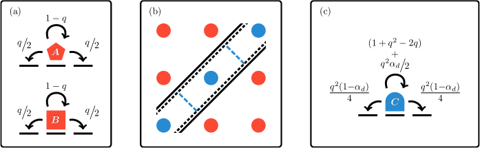
Figure 14: Schematic representation of a two-particle coalescing process, modelled as one dimensional interacting random walkers. Panel (a) depicts the dynamics of particles $\bm{A}$ and $\bm{B}$ where $q\in(0,1]$ is the probability of moving at each time step. The combined dynamics of $\bm{A}$ and $\bm{B}$ can be represented via one next-nearest random walker in a 2D domain. This abstract domain is depicted in panel (b). The red circles represent locations where the two particles are on different sites, while the blue circles along the right diagonal are locations where they are co-located. In this space the interaction of $\bm{A}$ and $\bm{B}$ is modelled with partially reflecting barriers. The placement of these barriers are illustrated by the solid, dashed, and blue-dashed lines, the precise locations and permeability are given in Section C.2. The solid black lines are heterogeneities used to model the binding interactions, while the dashed black lines are used to control the unbinding interactions. The movement of $\bm{C}$ is represented by the 2D random walker moving along the diagonal. Its movement is slowed down, relative to $\bm{A}$ and $\bm{B}$, through the placement of partially reflecting barriers along the diagonal depicted by the dashed blue lines. The resulting movement dynamics of the complex $\bm{C}$ is shown in panel (c), where $\alpha_{c}\in[0,1]$ represents the degree with which the movement of the complex $\bm{C}$ is slowed down.

Coalescing processes are ubiquitous in biology and chemistry; they consist of two or more entities that interact to bind and form a new one with different movement characteristics. An example of a coalescing process is the search of a promoter region on DNA by transcription factors. These movement dynamics alternates between periods of 3D search in the cytoplasm and periods of restricted search along the 1D DNA [70]. We use our framework to study a system of relevance to the latter scenario: a first-passage process of two interacting particle in 1D.

We consider two particles labelled $\bm{A}$ and $\bm{B}$ that move independently on a 1D lattice with reflecting boundary conditions (see Fig. 14 for a schematic representation of the process). Their combined dynamics is described by a two dimensional next-nearest propagator $\varphi_{{\bm{n}_{0}}}{({\bm{n}},{t})}$, with $\bm{n}_{0}=(n_{0_{1}},n_{0_{2}})$ and $\bm{n}=(n_{{}_{1}},n_{{}_{2}})$. It represents the probability that the particle $\bm{A}$ and $\bm{B}$ are located, respectively, on the site $n_{{}_{1}}$ and $n_{{}_{2}}$ at time $t$ given that they started, respectively, on $n_{0_{1}}$, and $n_{0_{2}}$. Two particles instantaneously form the complex $\bm{C}$, namely when they encounter each other, that is when $\bm{n}=(m,m)$ for $1\leq m\leq N$.

The interactions between particles is modelled through the placement of heterogeneities on the combined 2D lattice, yielding three control parameters, $\alpha_{e}\in[0,1]$, $\alpha_{u}\in[0,1]$, and $\alpha_{c}\in[0,1]$ (see Section C.2 for details regarding the placement of the defects). These parameters are used to constrain, respectively, the binding events via mutual exclusion of $\bm{A}$ and $\bm{B}$, the unbinding events of $\bm{C}$ and the mobility of $\bm{C}$. The parameter $\alpha_{u}$ is proportional to the unbinding probabilities, while $\alpha_{e}$ is proportional to the mutual exclusion probability. When $\alpha_{u}=1$ and $\alpha_{e}=0$, there is no interaction between the two particles. The other extreme represents strong interaction: when $\alpha_{e}=1$ there is mutual exclusion, whereas $\alpha_{u}=0$ results in a binding that is irreversible. The parameter $\alpha_{c}\in[0,1]$ represents the fraction of the movement probability of complex $\bm{C}$ relative to the movement probability of the constituent particles $\bm{A}$ and $\bm{B}$. When $\alpha_{c}=1$ there is no slowing down, while $\alpha_{c}=0$ results in an immobile $\bm{C}$.

In Fig. 15 we plot the log ratios of the MFPT, $\mathfrak{F}_{{\bm{n}_{0}}\to{\bm{n}}}$ for both particles to reach a site at the same time, compared with the 2D homogeneous next-nearest neighbour analogue, $\mathcal{F}_{{\bm{n}_{0}}\to{\bm{n}}}$. The latter corresponds with the case when $\alpha_{e}=0$ and $\alpha_{u}=\alpha_{c}=1$. The panels (a)-(d) depict $\mathfrak{F}_{{\bm{n}_{0}}\to{\bm{n}}}$ for increasing values of $\alpha_{e}$. The smallest ratios are observed in the upper left quadrant, which corresponds with high cohesiveness of the complex $\bm{C}$ and with only a slight reduction to its mobility, given respectively by, low values of $\alpha_{u}$ and high values of $\alpha_{c}$. Within this parameter region, once the two particles bind they rarely separate, consequently the search in 2D reduces to a search in 1D with fewer sites to explore leading to smaller $\mathfrak{F}_{{\bm{n}_{0}}\to{\bm{n}}}$.

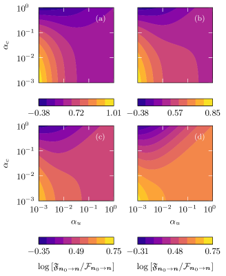
Figure 15: The ratio of the MFPT ($\mathfrak{F}_{{\bm{n}_{0}}\to{\bm{n}}}$) of the coalescing system compared to the MFPT ($\mathcal{F}_{{\bm{n}_{0}}\to{\bm{n}}}$) of a homogeneous 2D next-nearest neighbour walker as a function of the heterogeneity strength parameters (see Fig. 14 for detailed a description of the parameters involved). The reactive site is located at $\bm{n}=(100,100)$ and the two particles are initially maximal distance away from each other, i.e. $\bm{n}_{0}=(1,100)$ and a target location $\bm{n}=(100,100)$, on combined 2D domain of size $\bm{N}=(100,100)$ with diffusion parameter $q=2/3$. From panel (a) to (d) we have, respectively, the parameters $\alpha_{e}=0,0.5,0.75$ and $0.875$.

When there is no exclusion interaction, i.e. panel (a), the dynamics of a similar model was explored in Ref. [57]. In their analysis using asymptotics and simulations, equivalent features were observed. The most prominent feature of those and our observations is the minimisation of the MFPT for a slow moving $\bm{C}$. In this regime, it is more favourable to have an intermediate unbinding probability, allowing the two particles to travel independently towards the target before recombining and hitting the target.

The ability to explore easily the parameter space of the model allows us to analyse the MFPT for different values of $\alpha_{e}$. By comparing the four panels we observe that as $\alpha_{e}$ increases, the overall magnitude of the MFPT ratio decreases. This is explained by the fact that for small and intermediate values of $\alpha_{e}$ the 2D walker is partially restricted to the upper or lower triangular regions of the domain, thereby reducing the overall exploratory space resulting in shorter search times. However, if $\alpha_{e}$ is increased further, i.e. when $0\ll\alpha_{e}<1$, the particles will rarely coalesce, and the MFPT increases. In other words, shorter MFPTs can be achieved by having particles that mutually exclude one another with some probability.

VIII Conclusion

We have introduced an analytical framework to model explicitly any inert particle-environment interactions. We have constructed the discrete Master equation that describes the spatiotemporal dynamics of diffusing particles in disordered environments by representing the interactions as perturbed transition dynamics between lattice sites. To solve this Master equation we have extended the defect technique to yield the generating function of the propagator in closed form. Using the propagator, we have derived useful quantities in the context of transport processes, namely, first-passage, return and exit probabilities and their respective means. We have also uncovered the existence of a disorder indifference phenomenon of the mean first-passage time in quasi 1D systems.

In light of the relevance of our framework to empirical scenarios, we have chosen three examples to demonstrate its applicability of our theory. In the first example we consider transdermal drug delivery, an intercelluar transport process, where we represent the ‘brick-and-mortar’ structure of the stratum corneum with the placement of reflecting and partially reflecting barriers. This representation allows us to study the effect that piercing has on the traversal time of a drug molecule. In the second example, we have examined the effect that an animal’s thigomotactic response has on the mean squared displacement at log times. Lastly, in our third example, we have highlighted the ability of our formalism to study inert interactions between particles. We transformed these interactions and the ensuing dynamics into a single particle moving and interacting with quenched disorder in a higher dimensional space. The setup allows us to model analytically the search statistics in a two particle coalescing process, akin to the search of binding sites on the DNA by multiple transcription factors.

The strength of our result is in deriving the propagator in the presence of spatial heterogeneities, $\widetilde{\Phi}_{{\bm{n}_{0}}}{({\bm{n}},z)}$, as a function of the homogeneous propagator, i.e. the propagator in the absence of heterogeneities, $\widetilde{\varphi}_{{\bm{n}_{0}}}{({\bm{n}},z)}$. This modularity allows one to change the movement dynamics by selecting different forms of $\widetilde{\varphi}_{{\bm{n}_{0}}}{({\bm{n}},z)}$. In place of the diffusive propagator one may employ a biased lattice random walk [71], or a walk in different topologies such as triangular lattices [72, 73], Bethe lattices [74, 75] or more generally a network [76].

The modularity carries through to the heterogeneous propagator. This means that in situations where homogeneous space is assumed, one can relax this assumption and replace the homogeneous propagator, $\widetilde{\varphi}_{{\bm{n}_{0}}}{({\bm{n}},z)}$ with the heterogeneous counterpart $\widetilde{\Phi}_{{\bm{n}_{0}}}{({\bm{n}},z)}$. We have demonstrated this aspect by studying the first-passage probability to either of two targets using results previously derived considering a homogeneous lattice. Further theoretical exploration could include the analysis of cover time statistics [77, 78], transmission dynamics [79, 80], resetting walks [81, 82, 83], mortal walks [84], or random walks with internal degrees of freedom [85].

Directions for future applications span across spatial and temporal scales: the role of a building geometry or floor plan on infection dynamics in hospital wards and supermarkets [86, 87, 88]; the prediction of search pattern behaviour of animals in different types of vegetation cover [89, 90]; the heat transfer through layers of skin with differing thermal properties [91]; and the influence of topological defects on the diffusive properties in crystals [92, 93] and territorial systems [94, 95, 96].

We conclude by drawing the reader’s attention to the following. As experimental technologies continue to evolve, observations of the dynamics of particle-environment interactions are increasing in number and resolution. The detailed description of the environment that these technologies bring presents a unique opportunity to rethink modelling techniques, moving away from macroscopic paradigms to a more microscopic prescription. We believe that the mathematical framework we have introduced to quantify the particle-environment interactions will play a crucial role in connecting the microscopic dynamics to the macroscopic patterns observed across a vast array of systems.

Appendix A Mean First-Passage Statistics

Using the renewal equation the first-passage probability to a target is given by the well-known relation

$$\widetilde{\mathbb{F}}_{\bm{n}_{0}}(\bm{n},z) =\frac{\widetilde{\Phi}_{\bm{n}_{0}}(\bm{n},z)}{\widetilde{\Phi}_{\bm{n}}(\bm{n},z)}$$ (14)

$$=\frac{\left(\widetilde{\varphi}_{\bm{n}_{0}}(\bm{n},z)-1\right)\left|\underline{\bm{H}}\right|+\left|\underline{\bm{H}}{\left({\bm{n}},{\bm{n}_{{0}}}\right)}\right|}{\left(\widetilde{\varphi}_{\bm{n}}(\bm{n},z)-1\right)\left|\underline{\bm{H}}\right|+\left|\underline{\bm{H}}{\left({\bm{n}},{\bm{n}}\right)}\right|},$$

where $\underline{\bm{H}}$ and $\underline{\bm{H}}{\left({\bm{n}},{\bm{n}_{{0}}}\right)}$ are given by, respectively, Eqs. (III), (III) and (III) with the initial condition being $\bm{n}$. The mean of the distribution, $\mathfrak{F}_{{\bm{n}_{0}}\to{\bm{n}}}=\left.\frac{\mathrm{d}}{\mathrm{d}z}\widetilde{\mathbb{F}}_{{\bm{n}_{0}}}{({\bm{n}},z)}\right|_{z=1}$, (see LABEL:sup-sec:mret_deriv of the Supplementary Materials) is given by

$$\begin{split}\mathfrak{F}_{\bm{n}_{0}\to\bm{n}}=\frac{\mathcal{F}_{{\bm{n}_{0}}\to{\bm{n}}}\left|\underline{\bm{\mathcal{H}}}-1/\mathcal{F}_{{\bm{n}_{0}}\to{\bm{n}}}\underline{\bm{\mathcal{H}}}^{{({1})}}\right|}{\left|\underline{\bm{\mathcal{H}}}-\underline{\bm{\mathcal{H}}}^{{({2})}}\right|}.\end{split}$$ (15)

where

$$\underline{\bm{\mathcal{H}}}_{i,j} =\frac{\lambda_{{{\bm{\varvb}}}_{{i}},{{\bm{u}}}_{{i}}}}{\mathcal{R}_{\bm{u}_{i}}}\mathcal{F}_{\left\langle\bm{u}_{j}-\bm{\varvb}_{j}\right\rangle\to\bm{u}_{i}}-\frac{\lambda_{{{\bm{u}}}_{{i}},{{\bm{\varvb}}}_{{i}}}}{\mathcal{R}_{\bm{\varvb}_{i}}}\mathcal{F}_{\left\langle\bm{u}_{j}-\bm{\varvb}_{j}\right\rangle\to\bm{\varvb}_{i}}+\delta_{i,j},$$ (16)

$$\underline{\bm{\mathcal{H}}}^{{({1})}}_{i,j} =\left(\frac{\lambda_{{{\bm{\varvb}}}_{{i}},{{\bm{u}}}_{{i}}}}{\mathcal{R}_{\bm{u}_{i}}}\mathcal{F}_{\left\langle\bm{n}_{0}-\bm{n}\right\rangle\to\bm{u}_{i}}-\frac{\lambda_{{{\bm{u}}}_{{i}},{{\bm{\varvb}}}_{{i}}}}{\mathcal{R}_{\bm{\varvb}_{i}}}\mathcal{F}_{\left\langle\bm{n}_{0}-\bm{n}\right\rangle\to\bm{\varvb}_{i}}\right)$$ (17)

$$\times\mathcal{F}_{\left\langle\bm{u}_{j}-\bm{\varvb}_{j}\right\rangle\to\bm{n}},$$

$$\underline{\bm{\mathcal{H}}}^{{({2})}}_{i,j} =\left(\frac{\lambda_{{{\bm{\varvb}}}_{{i}},{{\bm{u}}}_{{i}}}}{\mathcal{R}_{\bm{u}_{i}}}-\frac{\lambda_{{{\bm{u}}}_{{i}},{{\bm{\varvb}}}_{{i}}}}{\mathcal{R}_{\bm{\varvb}_{i}}}\right)\mathcal{F}_{\left\langle\bm{u}_{j}-\bm{\varvb}_{j}\right\rangle\to\bm{n}}.$$ (18)

If the homogeneous propagator is diffusive with no bias and if the heterogeneity parameters are symmetric, i.e. $\lambda_{{{\bm{\varvb}}},{{\bm{u}}}}=\lambda_{{{\bm{u}}},{{\bm{\varvb}}}}$, $\underline{\bm{\mathcal{H}}}^{{({2})}}=0$ and Eq. 8 can be simplified further

$$\mathfrak{F}_{{\bm{n}_{0}}\to{\bm{n}}}=\mathcal{F}_{{\bm{n}_{0}}\to{\bm{n}}}-1+\frac{\left|\underline{\bm{\mathcal{H}}}-\underline{\bm{\mathcal{H}}}^{{({1})}}\right|}{\left|\underline{\bm{\mathcal{H}}}\right|}.$$ (19)

A.1 Mean Return Time

Through the renewal equation we also have the return probability relation

$$\widetilde{\mathbb{R}}{({\bm{n}},z)} =1-\frac{1}{\widetilde{\Phi}_{\bm{n}}(\bm{n},z)}$$ (20)

$$=\frac{\left(\widetilde{\varphi}_{{\bm{n}}}{({\bm{n}},z)}-2\right)\left|\underline{\bm{H}}\right|+\left|\underline{\bm{H}}{\left({\bm{n}},{\bm{n}}\right)}\right|}{\left(\widetilde{\varphi}_{{\bm{n}}}{({\bm{n}},z)}-1\right)\left|\underline{\bm{H}}\right|+\left|\underline{\bm{H}}{\left({\bm{n}},{\bm{n}}\right)}\right|}.$$

By noticing the identical structures of Eqs. 14 and 20, one can use a similar procedure to the one used to derive the MFPT (see LABEL:sup-sec:mret_deriv of the Supplementary Materials) to show the mean return time (MRT) to be

$$\mathfrak{R}_{\bm{n}}=\frac{\mathcal{R}_{\bm{n}}\left|\underline{\bm{\mathcal{H}}}\right|}{\left|\underline{\bm{\mathcal{H}}}-\underline{\bm{\mathcal{H}}}^{{({2})}}\right|}.$$ (21)

A.2 Mean Exit Times

The first-exit probability is given by $\widetilde{\mathbb{E}}_{{\bm{n}_{0}}}{(z)}=1-(1-z)\widetilde{\mathbb{S}}_{{\bm{n}_{0}}}{(z)}$, where $\widetilde{\mathbb{S}}_{{\bm{n}_{0}}}{(z)}$ is the survival probability given by

$$\widetilde{\mathbb{S}}_{{\bm{n}_{0}}}{(z)}=\sum_{\bm{n}}\widetilde{\Phi}_{{\bm{n}_{0}}}{({\bm{n}},z)}.$$ (22)

Substituting Eq. 5 into Eq. 22 and evaluating the sum in $\bm{n}$ and simplifying the summation over $k$ one finds

$$\widetilde{\mathbb{S}}_{{\bm{n}_{0}}}{(z)}=\widetilde{S}_{{\bm{n}_{0}}}{(z)}-1+\frac{\left|\underline{\bm{H}}-\underline{\bm{S}}{\left({\bm{n}_{{0}}}\right)}\right|}{\left|\underline{\bm{H}}\right|}$$ (23)

where $\widetilde{S}_{{\bm{n}_{0}}}{(z)}=\sum_{\bm{n}}\widetilde{\varphi}_{{\bm{n}_{0}}}{({\bm{n}},z)}$ is the homogeneous survival probability, and where the elements of $\underline{\bm{H}}$ are given in Section III and

$$\underline{\bm{S}}{\left({\bm{n}_{{0}}}\right)}_{i,j} =\widetilde{S}_{{\left\langle\bm{u}_{j}-\bm{\varvb}_{j}\right\rangle}}{(z)}\left[\lambda_{{{\bm{\varvb}}}_{{i}},{{\bm{u}}}_{{i}}}\widetilde{\varphi}_{{\bm{n}_{0}}}{({\bm{u}_{i}},z)}\right.$$ (24)

$$\left.\phantom{\widetilde{S}_{{\left\langle\bm{u}_{j}-\bm{\varvb}_{j}\right\rangle}}{(z)}}-\lambda_{{{\bm{u}}}_{{i}},{{\bm{\varvb}}}_{{i}}}\widetilde{\varphi}_{{\bm{n}_{0}}}{({\bm{\varvb}_{i}},z)}\right].$$

By taking the mean of the first-exit distribution, i.e. $\left.\frac{\mathrm{d}}{\mathrm{d}z}\widetilde{\mathbb{E}}_{{\bm{n}_{0}}}{(z)}\right|_{z=1}$ gives Eq. 10. The mathematical details to derive Eq. 10 are given in Section A.2 while simple expressions of the 1D problem are given in LABEL:sup-sec:expression_1d_suppl of the Supplementary materials.

Appendix B First-passage quantities in 1D systems

B.1 The MFPT disorder indifference phenomenon

We start with a heterogeneous lattice reflecting boundary between $n=0$ and $n=1$, and a partially reflecting barrier between $u$ and $u+1$, with $u<n_{0}<n$ as depicted in Fig. B1. The trajectories that contribute to the first-passage probability can be split into mutually exclusive sets based on the number of return visits, $m$, to the initial site $n_{0}$.

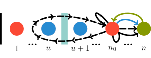
Figure B1: A schematic representation of a one dimensional heterogeneous lattice with a reflecting boundary to the left (vertical line) and with a permeable barrier between the sites $u$ and $u+1$ represented by the shaded rectangle. The first-passage event can be split into mutually exclusive events represented by arrows of different colours. The blue arrows represent trajectories that never return to the initial site, while the black ones represent trajectories that return $m$ times before reaching $n$. The green arrow represents first-passage trajectories that reach $n_{0}$ having starting at $n$. The solid arrows represent trajectories that are unaffected by the presence of the partially reflecting barrier between $u$ and $u+1$, while the trajectories that are affected are represented by dashed arrows. Note that this schematic depicts the case when $1\leq u\leq n_{0}-1$

We now formally represent the first-passage probability in terms of a set of mutually exclusive independent events. Let us define $F_{n_{0}}(n,t;m=0)$ as the first-passage probability to reach $n$ for the first time at $t$ having started at $n_{0}$ and having never returned to the initial site. Clearly, the trajectories that make up $F_{n_{0}}(n,t;m=0)$ (coloured blue in Fig. B1), can never be affected by the presence of the barrier as they never move towards the barrier. The trajectories that could be affected by the presence of the barrier are those that return at-least once to the initial site before reaching $n$. The first-passage probability to visit $n$ and having visited the initial site $m$ times is constructed through the convolution (dashed trajectories in Fig. B1)

$$\mathbb{F}_{n_{0}}(n,t;m)= \sum_{t_{{1}}=0}^{t}\cdots\sum_{t_{{m}}=0}^{t_{{m-1}}}F_{n_{0}}(n,t-t_{{1}};m=0)$$ (25)

$$\times h_{n_{0}}(n,t_{{m-1}}-t_{{m}})\cdots h_{n_{0}}(n,t_{{m}}),$$

with $t_{m}\leq t_{m-1}\leq\cdots\leq t_{1}\leq t$, and where

$$h_{n_{0}}(n,t) =\mathbb{R}(n_{0},{t})$$ (26)

$$-\sum_{{t^{\prime}}=0}^{t}F_{n_{0}}(n,{t^{\prime}};m=0)F_{n}(n_{0},{t}-{t^{\prime}})$$

The function $h_{n_{0}}(n,t)$ represents the probability of returning without visiting the target and is constructed by considering the probability of returning to $n_{0}$ and subtracting those that reach $n$ without returning to $n_{0}$ at some prior time and subsequently reaching $n_{0}$ from $n$. In $z$ domain the relation can be written more conveniently as

$$\widetilde{\mathbb{F}}_{n_{0}}(n,z;m) =\widetilde{F}_{n_{0}}(n,z;m=0)\left[\widetilde{\mathbb{R}}{({n_{0}},z)}\right.$$ (27)

$$\left.-\widetilde{F}_{n_{0}}(n,z;m=0)\widetilde{F}_{{n}}{({n_{0}},z)}\right]^{m}.$$

Notice that the only term with the dependence on the barrier on the RHS of Eq. 27 is $\widetilde{\mathbb{R}}{({n_{0}},z)}$, and in the absence of the barrier $\widetilde{\mathbb{R}}{({n_{0}},z)}$ reduces to $\widetilde{R}{({n_{0}},z)}$. The full first-passage probability for the system with the barrier, which can be written as the sum of the mutually exclusive probabilities giving

$$\widetilde{\mathbb{F}}_{{n_{0}}}{({n},z)} =\widetilde{F}_{n_{0}}(n,z;m=0)\sum^{\infty}_{m=0}\left[\widetilde{\mathbb{R}}{({n_{0}},z)}\right.$$ (28)

$$-\left.\widetilde{F}_{n_{0}}(n,z;m=0)\widetilde{F}_{{n}}{({n_{0}},z)}\right]^{m}.$$

The relation given by Eq. 28 is an alternative method of constructing the first-passage probability i.e. its not one of the standard approaches which are through the survival probability or the ratio of propagators in $z$-domain.

To confirm the normalisation of the RHS of Eq. 28 consider the following. By definition $F_{n_{0}}(n,t;m=0)$ is not normalised over $t$, hence, $\widetilde{F}_{n_{0}}(n,z=1;m=0)=p$ where $0<p<1$. Since all other terms in the RHS of Eq. 28, namely, $\widetilde{F}_{{n}}{({n_{0}},z)}$ and $\widetilde{\mathbb{R}}{({n_{0}},z)}$ are normalised over time, we find that at $z=1$ the RHS becomes $\sum_{m=0}^{\infty}p(1-p)^{m}=1$. Differentiating Eq. 28 with respect to $z$ and taking the limit $z\to 1$, we obtain the mean first-passage time

$$\mathfrak{F}_{{n_{0}}\to{n}}=\frac{\mathfrak{R}_{n}-p\mathcal{F}_{{n}\to{n_{0}}}}{p}.$$ (29)

When the barrier is such that $\lambda_{u,u+1}=\lambda_{u+1,u}=\lambda$ , the mean return time is equal to the reciprocal of the steady state value, and $\mathfrak{R}_{n_{0}}$ becomes $\mathcal{R}_{n_{0}}$, i.e. the mean return time in the absence of the barrier.

To find $p$ in Eq. 29 explicitly, we first construct $\widetilde{F}_{n_{0}}(n,z;m=0)$ in terms of known quantities using the approach presented in Ref. [58] to construct time-dependent splitting probabilities. We write the two relations by considering the two splitting separately: the first-passage probability of reaching the target $n$ and never returning to the initial condition $F_{n_{0}}(n,t;m=0)$; and the first-return probability to $n_{0}$ and having never reached the target site $n$. In time domain they are written via a convolution and are, respectively,

$$F_{n_{0}}(n,t;m=0)=F_{n_{0}}(n,t)-\sum_{t^{\prime}=0}^{t}\mathbb{R}(n_{0},t;n)F_{n_{0}}(n,t-t^{\prime})$$ (30)

and

$$\mathbb{R}(n_{0},t;n)=\mathbb{R}(n_{0},t)-\sum_{t^{\prime}=0}^{t}F_{n_{0}}(n,t;m=0)F_{n_{0}}(n,t-t^{\prime}),$$ (31)

where $\mathbb{R}(n_{0},t;n)$ is the probability of returning to the site $n_{0}$ at $t$ and having never visited the target $n$. One can take the $z$-transform and solve for $F_{n_{0}}(n,z;m=0)$ and $\mathbb{R}(n_{0},t;n)$ giving, respectively,

$$\widetilde{F}_{n_{0}}(n,z;m=0)=\frac{\widetilde{F}_{{n_{0}}}{({n},z)}-\widetilde{\mathbb{R}}(n_{0},z)\widetilde{F}_{{n_{0}}}{({n},z)}}{1-\widetilde{F}_{{n_{0}}}{({n},z)}\widetilde{F}_{{n}}{({n_{0}},z)}}$$ (32)

and

$$\widetilde{\mathbb{R}}(n_{0},z;n)=\frac{\widetilde{\mathbb{R}}(n_{0},z)-\widetilde{F}_{{n_{0}}}{({n},z)}\widetilde{F}_{{n}}{({n_{0}},z)}}{1-\widetilde{F}_{{n_{0}}}{({n},z)}\widetilde{F}_{{n}}{({n_{0}},z)}}.$$ (33)

Evaluating Eqs. 32 and 33 at $z=1$ gives, respectively, the fraction of all the first-passage trajectories that reach the target without returning to $n_{0}$ and the fraction of all trajectories that return to $n_{0}$ without ever reaching $n$. Using de L’Hôpital’s rule once in Eq. 32 we find

$$p =\frac{\mathfrak{R}_{n_{0}}}{\mathcal{F}_{{n_{0}}\to{n}}+\mathcal{F}_{{n}\to{n_{0}}}}.$$ (34)

Inserting Eq. 34 in Eq. 29 one finds that $\mathfrak{F}_{{n_{0}}\to{n}}=\mathcal{F}_{{n_{0}}\to{n}}$.

B.2 MFPT linear dependence on disorder location

To understand the linear dependence in $u$, with $n_{0}\leq u<n$, present in Eq. 12, we consider building up first passage probability by convolution in time to go from $n_{0}$ to $u$ first, then from $u$ to $u+1$ and then from $u+1$ to $n$. In $z$ domain one has

$$\widetilde{\mathbb{F}}_{{n_{0}}}{({n},z)}=\widetilde{F}_{{n_{0}}}{({u},z)}\widetilde{\mathbb{F}}_{{u}}{({u+1},z)}\widetilde{\mathbb{F}}_{{u+1}}{({n},z)},$$ (35)

where the first term on the RHS has no dependence on the barrier as it is after the absorbing site $u$, while the other two terms are dependent on the barrier. Computing the mean of Eq. 35, we obtain

$$\mathfrak{F}_{{n_{0}}\to{n}}=\mathcal{F}_{{n_{0}}\to{u}}+\mathfrak{F}_{{u}\to{u+1}}+\mathcal{F}_{{u+1}\to{n}},$$ (36)

where we have substituted $\mathfrak{F}_{{u+1}\to{n}}=\mathcal{F}_{{u+1}\to{n}}$ using the justification presented in the previous section. By using the relation $\mathcal{F}_{{n_{0}}\to{n}}=\mathcal{F}_{{n_{0}}\to{s}}+\mathcal{F}_{{s}\to{n}}$ with $n_{0}<s<n$, one can rewrite Eq. 36 to give

$$\mathfrak{F}_{{n_{0}}\to{n}}=\mathcal{F}_{{n_{0}}\to{n}}+\mathfrak{F}_{{u}\to{u+1}}-\mathcal{F}_{{u}\to{u+1}}.$$ (37)

In the diffusive case, the MFPT to a neighbouring site, $\mathcal{F}_{{u}\to{u+1}}$, is always proportional to twice the distance between $u$ and the reflecting boundary to the left, i.e.

$$\mathcal{F}_{{u}\to{u+1}}=\frac{2}{q}(u-s+1),$$ (38)

with $s\leq u$ being the position of the reflecting boundary. By simplifying the general MFPT given in Eq. 8, we find

$$\mathfrak{F}_{{u}\to{u+1}}=\frac{2}{q-2\lambda}\left(u-s+1\right),$$ (39)

which is analogous to Eq. 38 but with the multiplicative (time rescale) factor increased to $2(q-2\lambda)^{-1}$. Letting $s=1$ we obtain Eq. 12.

Appendix C Placement of Defects and Parameter Choice of the Modelling Applications

C.1 Thigmotaxis

Two sets of defects must be placed, one set along a circle radius $R$ to create a (circular) reflecting domain, while the second is used to divide this domain into two different regions (see Section VI) and is placed along a circle of radius $r$. To place defects on either circle one must first know which sites are within which circle. To determine this we use the Euclidean distance as a heuristic, with the site $\bm{n}=(n_{1},n_{2})$ being part of the circular domain if and only if $h(n_{1},n_{2})\leq R$, where $h(n_{1},n_{2})=\left[{(n_{1}-R-1)}^{2}+{(n_{2}-R-1)}\right]^{1/2}$ with the size of the bounding square domain given by $\bm{N}=(2R+1,2R+1)$. Similarly, a site is part of the inner region if and only if $h(n_{1},n_{2})\leq r$, while the outer region is given by $r<h(n_{1},n_{2})\leq R$. Given these site partitions, one can define two sets of defects, $S_{{d}}$, and $S_{{i}}$ describing, respectively, the impenetrable barriers to restrict the walker to a circular domain, and partially-reflecting inner barriers. In both cases $\bm{u}$ represents sites inside the circle of defects while $\bm{\varvb}$ represents sites outside. For all $\left\{\bm{u},\bm{\varvb}\right\}\in S_{{i}}$ we have $\lambda_{{{\bm{\varvb}}},{{\bm{u}}}}=\underline{\bm{A}}_{{\bm{\varvb}},{\bm{u}}}$ and $\lambda_{{{\bm{u}}},{{\bm{\varvb}}}}$ is irrelevant as the walker initially starts inside the circular domain. For all $\left\{\bm{u},\bm{\varvb}\right\}\in S_{{d}}$, we let $\lambda_{{{\bm{\varvb}}},{{\bm{u}}}}=0$ providing no resistance for the walker to enter the outer-region and $\lambda_{{{\bm{u}}},{{\bm{\varvb}}}}=\alpha_{{i}}\underline{\bm{A}}_{{\bm{u}},{\bm{\varvb}}}$ with $\alpha_{{i}}\in[0,1]$.

C.2 Two particle coalescing process

The interactions that need to modelled are binding and unbinding. Binding can occur via two distinct events. The first is when two particles are located on neighbouring sites with $\bm{n}=(m+1,m)$ and at the following time step, one of the particles remains at the same site while the second particle jumps onto the site occupied by the first resulting in $\bm{n}=(m+1,m+1)$ or $\bm{n}=(m,m)$. The second possible event occurs when the two particles are located two sites apart i.e. $\bm{n}=(m-1,m+1)$ and at the following time step they both jump towards each other landing on $\bm{n}=(m,m)$. The reverse of these two events gives rise to unbinding of the complex $\bm{C}$. These transitions can be modified by placing paired defects of the forms: $\bm{u}=(m,m)$, $\bm{\varvb}=(m+1,m)$, and $\bm{u}=(m,m)$, $\bm{\varvb}=(m,m+1)$ for $1\leq m\leq N-1$ with $\lambda_{{{\bm{\varvb}}},{{\bm{u}}}}=\frac{q}{2}(1-q)(1-\alpha_{u})$, $\lambda_{{{\bm{u}}},{{\bm{\varvb}}}}=\frac{q}{2}(1-q)\alpha_{e}$; $\bm{u}=(m,m)$ , $\bm{\varvb}=(m,m-1)$ and $\bm{u}=(m,m)$ , $\bm{\varvb}=(m-1,m)$ for $2\leq m\leq N$ with $\lambda_{{{\bm{\varvb}}},{{\bm{u}}}}=\frac{q}{2}(1-q)(1-\alpha_{u})$, $\lambda_{{{\bm{u}}},{{\bm{\varvb}}}}=\frac{q}{2}(1-q)\alpha_{e}$; $\bm{u}=(m,m)$, $\bm{\varvb}=(m\mp 1,m\pm 1)$ for $2\leq m\leq N-1$ with $\lambda_{{{\bm{\varvb}}},{{\bm{u}}}}=\frac{q^{2}}{4}(1-\alpha_{u})$, $\lambda_{{{\bm{u}}},{{\bm{\varvb}}}}=\frac{q^{2}}{4}\alpha_{e}$.

Intuitively, the movement of the coalesced is slowed as it more massive. To encode this detail we interpret jumps along the leading diagonal $\bm{n}=(m,m)$ for all $1\leq m\leq N$ as the jumps made by the coalesced particle $\bm{C}$, and we slow its movement by placing paired defects of the form $\bm{u}=(m,m)$, $\bm{\varvb}=(m+1,m+1)$ for all $1\leq m\leq N-1$ with $\lambda_{{{\bm{\varvb}}},{{\bm{u}}}}=\lambda_{{{\bm{u}}},{{\bm{\varvb}}}}=\frac{q^{2}}{4}(1-\alpha_{c})$.

References

- Fischer and Hertz [1991] K. H. Fischer and J. A. Hertz, Spin Glasses, Cambridge Studies in Magnetism (Cambridge University Press, Cambridge, 1991).
- Amro et al. [2000] N. A. Amro, L. P. Kotra, K. Wadu-Mesthrige, A. Bulychev, S. Mobashery, and G.-y. Liu, High-resolution atomic force microscopy studies of the escherichia coli outer membrane: Structural basis for permeability, Langmuir 16, 2789 (2000).
- Buxton and Clarke [2006] G. A. Buxton and N. Clarke, Computer simulation of polymer solar cells, Model. Simul. Mater. Sc. 15, 13 (2006).
- Beyer et al. [2016] H. L. Beyer, E. Gurarie, L. Börger, M. Panzacchi, M. Basille, I. Herfindal, B. Van Moorter, S. R. Lele, and J. Matthiopoulos, ‘you shall not pass!’: Quantifying barrier permeability and proximity avoidance by animals, J. Anim. Ecol. 85, 43 (2016).
- Assis et al. [2019] J. C. Assis, H. C. Giacomini, and M. C. Ribeiro, Road permeability index: Evaluating the heterogeneous permeability of roads for wildlife crossing, Ecol. Indic. 99, 365 (2019).
- Seebauer and Noh [2010] E. G. Seebauer and K. W. Noh, Trends in semiconductor defect engineering at the nanoscale, Materials Science and Engineering: R: Reports 3rd IEEE International NanoElectronics Conference (INEC), 70, 151 (2010).
- Bai et al. [2018] S. Bai, N. Zhang, C. Gao, and Y. Xiong, Defect engineering in photocatalytic materials, Nano Energy 53, 296 (2018).
- Jeltsch et al. [2013] F. Jeltsch, D. Bonte, G. Pe’er, B. Reineking, P. Leimgruber, N. Balkenhol, B. Schröder, C. M. Buchmann, T. Mueller, N. Blaum, D. Zurell, K. Böhning-Gaese, T. Wiegand, J. A. Eccard, H. Hofer, J. Reeg, U. Eggers, and S. Bauer, Integrating movement ecology with biodiversity research - exploring new avenues to address spatiotemporal biodiversity dynamics, Mov. Ecol. 1, 6 (2013).
- Silveira et al. [2016] N. S. D. Silveira, B. B. S. Niebuhr, R. d. L. Muylaert, M. C. Ribeiro, and M. A. Pizo, Effects of land cover on the movement of frugivorous birds in a heterogeneous landscape, PLOS One 11, e0156688 (2016).
- Fujiwara et al. [2002] T. Fujiwara, K. Ritchie, H. Murakoshi, K. Jacobson, and A. Kusumi, Phospholipids undergo hop diffusion in compartmentalized cell membrane, J. Cell Biol. 157, 1071 (2002).
- Fujiwara et al. [2016] T. K. Fujiwara, K. Iwasawa, Z. Kalay, T. A. Tsunoyama, Y. Watanabe, Y. M. Umemura, H. Murakoshi, K. G. N. Suzuki, Y. L. Nemoto, N. Morone, and A. Kusumi, Confined diffusion of transmembrane proteins and lipids induced by the same actin meshwork lining the plasma membrane, Mol. Biol. Cell 27, 1101 (2016).
- McGuffee and Elcock [2010] S. R. McGuffee and A. H. Elcock, Diffusion, crowding & protein stability in a dynamic molecular model of the bacterial cytoplasm, PLOS Comput. Biol. 6, e1000694 (2010).
- Dyson [1953] F. J. Dyson, The dynamics of a disordered linear chain, Phys. Rev. 92, 1331 (1953).
- Schmidt [1957] H. Schmidt, Disordered one-dimensional crystals, Phys. Rev. 105, 425 (1957).
- Halperin [1965] B. I. Halperin, Green’s functions for a particle in a one-dimensional random potential, Phys. Rev. 139, A104 (1965).
- Lieb [1981] E. H. Lieb, Mathematical Physics in One Dimension: Exactly Soluble Models of Interacting Particles a Collection of Reprints with Introductory Text, 3rd ed., Perspectives in Physics (Acad. Pr, New York, 1981).
- Hori [1968] J. Hori, Spectral Properties of Disordered Chains and Lattices, 1st ed. (Pergamon Press, 1968).
- Havlin and Ben-Avraham [1987] S. Havlin and D. Ben-Avraham, Diffusion in disordered media, Adv. Phys. 36, 695 (1987).
- Zwanzig [1982] R. Zwanzig, Non-markoffian diffusion in a one-dimensional disordered lattice, J. Stat. Phys. 28, 127 (1982).
- Alexander et al. [1981] S. Alexander, J. Bernasconi, W. R. Schneider, and R. Orbach, Excitation dynamics in random one-dimensional systems, Rev. Mod. Phys. 53, 175 (1981).
- Sinai [1983] Y. G. Sinai, The limiting behavior of a one-dimensional random walk in a random medium, Theory Probab. Appl. 27, 256 (1983).
- Durrett [1986] R. Durrett, Multidimensional random walks in random environments with subclassical limiting behavior, Commun. Math. Phys. 104, 87 (1986).
- Blumberg Selinger et al. [1989] R. L. Blumberg Selinger, S. Havlin, F. Leyvraz, M. Schwartz, and H. E. Stanley, Diffusion in the presence of quenched random bias fields: A two-dimensional generalization of the sinai model, Phys. Rev. A 40, 6755 (1989).
- Murthy and Kehr [1989] K. P. N. Murthy and K. W. Kehr, Mean first-passage time of random walks on a random lattice, Phys. Rev. A 40, 2082 (1989).
- Hughes [1996] B. D. Hughes, Random Walks and Random Environments: Volume 2: Random Environments (OUP Oxford, Oxford, 1996).
- Haus and Kehr [1987] J. W. Haus and K. W. Kehr, Diffusion in regular and disordered lattices, Phys. Rep. 150, 263 (1987).
- Bressloff and Newby [2013] P. C. Bressloff and J. M. Newby, Stochastic models of intracellular transport, Rev. Mod. Phys. 85, 135 (2013).
- Metzler et al. [2014] R. Metzler, J.-H. Jeon, A. G. Cherstvy, and E. Barkai, Anomalous diffusion models and their properties: Non-stationarity, non-ergodicity, and ageing at the centenary of single particle tracking, Phys. Chem. Chem. Phys. 16, 24128 (2014).
- Meroz and Sokolov [2015] Y. Meroz and I. M. Sokolov, A toolbox for determining subdiffusive mechanisms, Phys. Rep. 573, 1 (2015).
- Höfling and Franosch [2013] F. Höfling and T. Franosch, Anomalous transport in the crowded world of biological cells, Rep. Prog. Phys. 76, 046602 (2013).
- Meyer et al. [2012] B. Meyer, O. Bénichou, Y. Kafri, and R. Voituriez, Geometry-induced bursting dynamics in gene expression, Biophys. J. 102, 2186 (2012).
- Chubynsky and Slater [2014] M. V. Chubynsky and G. W. Slater, Diffusing diffusivity: A model for anomalous, yet brownian, diffusion, Phys. Rev. Lett. 113, 098302 (2014).
- Lanoiselée and Grebenkov [2018] Y. Lanoiselée and D. S. Grebenkov, A model of non-gaussian diffusion in heterogeneous media, J. Phys. A: Math. Theor. 51, 145602 (2018).
- Sposini et al. [2018] V. Sposini, A. Chechkin, and R. Metzler, First passage statistics for diffusing diffusivity, J. Phys. A: Math. Theor. 52, 04LT01 (2018).
- Lanoiselée et al. [2018] Y. Lanoiselée, N. Moutal, and D. S. Grebenkov, Diffusion-limited reactions in dynamic heterogeneous media, Nat. Commun. 9, 4398 (2018).
- Wang et al. [2012] B. Wang, J. Kuo, S. C. Bae, and S. Granick, When brownian diffusion is not gaussian, Nat. Mater. 11, 481 (2012).
- Metzler [2017] R. Metzler, Gaussianity fair: The riddle of anomalous yet non-gaussian diffusion, Biophys. J. 112, 413 (2017).
- Lampo et al. [2017] T. J. Lampo, S. Stylianidou, M. P. Backlund, P. A. Wiggins, and A. J. Spakowitz, Cytoplasmic rna-protein particles exhibit non-gaussian subdiffusive behavior, Biophys. J. 112, 532 (2017).
- Korabel and Barkai [2011] N. Korabel and E. Barkai, Boundary conditions of normal and anomalous diffusion from thermal equilibrium, Phys. Rev. E 83, 051113 (2011).
- Godec and Metzler [2015] A. Godec and R. Metzler, Optimization and universality of brownian search in a basic model of quenched heterogeneous media, Phys. Rev. E 91, 052134 (2015).
- Vaccario et al. [2015] G. Vaccario, C. Antoine, and J. Talbot, First-passage times in d -dimensional heterogeneous media, Phys. Rev. Lett. 115, 240601 (2015).
- Godec and Metzler [2016] A. Godec and R. Metzler, Universal proximity effect in target search kinetics in the few-encounter limit, Phys. Rev. X 6, 041037 (2016).
- Powles et al. [1992] J. G. Powles, M. Mallett, G. Rickayzen, and W. Evans, Exact analytic solutions for diffusion impeded by an infinite array of partially permeable barriers, Proc. R. Soc. A: Math. Phys. Eng. Sci. 436, 391 (1992).
- Kenkre et al. [2008] V. M. Kenkre, L. Giuggioli, and Z. Kalay, Molecular motion in cell membranes: Analytic study of fence-hindered random walks, Phys. Rev. E 77, 051907 (2008).
- Kalay et al. [2008] Z. Kalay, P. E. Parris, and V. M. Kenkre, Effects of disorder in location and size of fence barriers on molecular motion in cell membranes, J. Phys. Condens. Matter 20, 245105 (2008).
- Grebenkov [2014] D. S. Grebenkov, Exploring diffusion across permeable barriers at high gradients. ii. localization regime, J. Magn. Reson. 248, 164 (2014).
- Moutal and Grebenkov [2019] N. Moutal and D. Grebenkov, Diffusion across semi-permeable barriers: Spectral properties, efficient computation, and applications, J. Sci. Comput. 81, 1630 (2019).
- Montroll and Potts [1955] E. W. Montroll and R. B. Potts, Effect of defects on lattice vibrations, Phys. Rev. 100, 525 (1955).
- Montroll and West [1979] E. W. Montroll and B. J. West, On an enriched collection of stochastic processes, in Studies in Statistical Mechanics: Vol VII. Fluctuation Phenomena, edited by E. Montroll and J. Lebowitz (North Holland Publishing, Amsterdam, 1979) pp. 61–175.
- Kenkre [2021] V. M. Kenkre, Memory Functions, Projection Operators, and the Defect Technique: Some Tools of the Trade for the Condensed Matter Physicist, Lecture Notes in Physics No. volume 982 (Springer, Cham, 2021).
- Bénichou and Voituriez [2014] O. Bénichou and R. Voituriez, From first-passage times of random walks in confinement to geometry-controlled kinetics, Phys. Rep. 539, 225 (2014).
- Prausnitz et al. [2004] M. R. Prausnitz, S. Mitragotri, and R. Langer, Current status and future potential of transdermal drug delivery, Nat. Rev. Drug Discov. 3, 115 (2004).
- Prausnitz and Langer [2008] M. R. Prausnitz and R. Langer, Transdermal drug delivery, Nat. Biotechnol. 26, 1261 (2008).
- Jeanson et al. [2003] R. Jeanson, S. Blanco, R. Fournier, J.-L. Deneubourg, V. Fourcassié, and G. Theraulaz, A model of animal movements in a bounded space, J. Theor. Biol. 225, 443 (2003).
- Miramontes et al. [2014] O. Miramontes, O. DeSouza, L. R. Paiva, A. Marins, and S. Orozco, Lévy flights and self-similar exploratory behaviour of termite workers: Beyond model fitting, PLOS One 9, e111183 (2014).
- Mirny et al. [2009] L. Mirny, M. Slutsky, Z. Wunderlich, A. Tafvizi, J. Leith, and A. Kosmrlj, How a protein searches for its site on dna: The mechanism of facilitated diffusion, J. Phys. A: Math. Theor. 42, 434013 (2009).
- Shin and Kolomeisky [2019] J. Shin and A. B. Kolomeisky, Target search on dna by interacting molecules: First-passage approach, J. Chem. Phys. 151, 125101 (2019).
- Giuggioli [2020] L. Giuggioli, Exact spatiotemporal dynamics of confined lattice random walks in arbitrary dimensions: A century after Smoluchowski and Pólya, Phys. Rev. X 10, 021045 (2020).
- Abate and Whitt [1992] J. Abate and W. Whitt, Numerical inversion of probability generating functions, Oper. Res. Lett. 12, 245 (1992).
- Abate et al. [2000] J. Abate, G. L. Choudhury, and W. Whitt, An introduction to numerical transform inversion and its application to probability models, in Computational Probability (Springer, 2000) pp. 257–323.
- Nathan and Giuggioli [2013] R. M. Nathan and L. Giuggioli, A milestone for movement ecology research, Move. Ecol. 1 (2013).
- Giuggioli et al. [2018] L. Giuggioli, I. Arye, A. Heiblum Robles, and G. A. Kaminka, From ants to birds: A novel bio-inspired approach to online area coverage (2018) pp. 31–43.
- Redner et al. [2014] S. Redner, R. Metzler, and G. Oshanin, First-Passage Phenomena and Their Applications (World Scientific, Singapore, 2014).
- Kac [1947] M. Kac, On the notion of recurrence in discrete stochastic processes, Bull. Amer. Math. Soc. 53, 1002 (1947).
- Elias [2007] P. M. Elias, The skin barrier as an innate immune element, Semin. Immunopathol. 29, 3 (2007).
- Nemes and Steinert [1999] Z. Nemes and P. M. Steinert, Bricks and mortar of the epidermal barrier, Exp. Mol. Med. 31, 5 (1999).
- Ramadon et al. [2021] D. Ramadon, M. T. C. McCrudden, A. J. Courtenay, and R. F. Donnelly, Enhancement strategies for transdermal drug delivery systems: Current trends and applications, Drug Delivery and Translational Research (2021).
- Higaki et al. [2018] A. Higaki, M. Mogi, J. Iwanami, L.-J. Min, H.-Y. Bai, B.-S. Shan, H. Kan-No, S. Ikeda, J. Higaki, and M. Horiuchi, Recognition of early stage thigmotaxis in morris water maze test with convolutional neural network, PloS one 13, e0197003 (2018).
- Doria et al. [2019] M. D. Doria, J. Morand-Ferron, and S. M. Bertram, Spatial cognitive performance is linked to thigmotaxis in field crickets, Anim. Behav. 150, 15 (2019).
- Iwahara and Kolomeisky [2021] J. Iwahara and A. B. Kolomeisky, Discrete-state stochastic kinetic models for target dna search by proteins: Theory and experimental applications, Biophys. Chem. 269, 106521 (2021).
- Sarvaharman and Giuggioli [2020] S. Sarvaharman and L. Giuggioli, Closed-form solutions to the dynamics of confined biased lattice random walks in arbitrary dimensions, Phys. Rev. E 102, 062124 (2020).
- Hughes [1995] B. D. Hughes, Random Walks and Random Environments: Volume 1: Random Walks, illustrated edition ed. (OUP Oxford, Oxford, 1995).
- Batchelor and Henry [2002] M. T. Batchelor and B. I. Henry, Exact solution for random walks on the triangular lattice with absorbing boundaries, J. Phys. A: Math. Gen. 35, 5951 (2002).
- Hughes and Sahimi [1982] B. D. Hughes and M. Sahimi, Random walks on the Bethe lattice, J. Stat. Phys. 29, 781 (1982).
- Hughes et al. [1983] B. D. Hughes, M. Sahimi, and H. Ted Davis, Random walks on pseudo-lattices, Physica A 120, 515 (1983).
- Masuda et al. [2017] N. Masuda, M. A. Porter, and R. Lambiotte, Random walks and diffusion on networks, Phys. Rep. 716, 1 (2017).
- Nemirovsky and Coutinho-Filho [1991] A. M. Nemirovsky and M. D. Coutinho-Filho, Lattice covering time in d dimensions: Theory and mean field approximation, Physica A 177, 233 (1991).
- Chupeau et al. [2015] M. Chupeau, O. Bénichou, and R. Voituriez, Cover times of random searches, Nat. Phys. 11, 844 (2015).
- Giuggioli et al. [2013] L. Giuggioli, S. Pérez-Becker, and D. P. Sanders, Encounter times in overlapping domains: Application to epidemic spread in a population of territorial animals, Phys. Rev. Lett. 110, 058103 (2013).
- Kenkre and Giuggioli [2021] V. M. Kenkre and L. Giuggioli, Theory of the Spread of Epidemics and Movement Ecology of Animals: An Interdisciplinary Approach Using Methodologies of Physics and Mathematics (Cambridge University Press, Cambridge, UK, 2021).
- Evans and Majumdar [2011] M. R. Evans and S. N. Majumdar, Diffusion with optimal resetting, J. Phys. A: Math. Theor. 44, 435001 (2011).
- Pal and Reuveni [2017] A. Pal and S. Reuveni, First passage under restart, Phys. Rev. Lett 118, 030603 (2017).
- Giuggioli et al. [2019] L. Giuggioli, S. Gupta, and M. Chase, Comparison of two models of tethered motion, J. Phys. A: Math. Theor. 52, 075001 (2019).
- Yuste et al. [2013] S. B. Yuste, E. Abad, and K. Lindenberg, Exploration and trapping of mortal random walkers, Phys. Rev. Lett. 110, 220603 (2013).
- Montroll [1969] E. W. Montroll, Random walks on lattices. iii. calculation of first-passage times with application to exciton trapping on photosynthetic units, J. Math. Phys. 10, 753 (1969).
- Qian et al. [2009] H. Qian, Y. Li, P. V. Nielsen, and X. Huang, Spatial distribution of infection risk of sars transmission in a hospital ward, Build. Environ. 44, 1651 (2009).
- Ying and O’Clery [2021] F. Ying and N. O’Clery, Modelling covid-19 transmission in supermarkets using an agent-based model, PLOS One 16, e0249821 (2021).
- Giuggioli and Sarvaharman [2022] L. Giuggioli and S. Sarvaharman, Spatio-temporal dynamics of random transmission events: from information sharing to epidemic spread, Journal of Physics A: Mathematical and Theoretical Under Review (2022).
- Crist et al. [1992] T. O. Crist, D. S. Guertin, J. A. Wiens, and B. T. Milne, Animal movement in heterogeneous landscapes: An experiment with eleodes beetles in shortgrass prairie, Funct. Ecol. 6, 536 (1992).
- Voigt et al. [2020] C. C. Voigt, J. M. Scholl, J. Bauer, T. Teige, Y. Yovel, S. Kramer-Schadt, and P. Gras, Movement responses of common noctule bats to the illuminated urban landscape, Landscape Ecol. 35, 189 (2020).
- Simpson et al. [2021] M. J. Simpson, A. P. Browning, C. Drovandi, E. J. Carr, O. J. Maclaren, and R. E. Baker, Profile likelihood analysis for a stochastic model of diffusion in heterogeneous media, Proc. R. Soc. A: Math. Phys. Eng. Sci. 477, 20210214 (2021).
- Bausch et al. [1994] R. Bausch, R. Schmitz, and L. A. Turski, Diffusion in the presence of topological disorder, Phys. Rev. Lett. 73, 2382 (1994).
- Chen and Deem [2003] L. Chen and M. W. Deem, Two-dimensional diffusion in the presence of topological disorder, Phys. Rev. E 68, 021107 (2003).
- Giuggioli and Kenkre [2014] L. Giuggioli and V. M. Kenkre, Consequences of animal interactions on their dynamics: Emergence of home ranges and territoriality, Mov. Ecol. 2 (2014).
- Heiblum Robles and Giuggioli [2018] A. Heiblum Robles and L. Giuggioli, Phase transitions in stigmergic territorial systems, Phys. Rev. E 98, 042115 (2018).
- Sarvaharman et al. [2019] S. Sarvaharman, A. Heiblum Robles, and L. Giuggioli, From micro-to-macro: How the movement statistics of individual walkers affect the formation of segregated territories in the territorial random walk model, Aip. Conf. Proc. 7, 129 (2019).