Data-Driven Output Prediction and Control of Stochastic Systems: An Innovation-Based Approach

Abstract

Recent years have witnessed a booming interest in data-driven control of dynamical systems. However, the implicit data-driven output predictors are vulnerable to uncertainty such as process disturbance and measurement noise, causing unreliable predictions and unexpected control actions. In this brief, we put forward a new data-driven approach to output prediction of stochastic LTI systems. By utilizing the innovation form, the uncertainty in stochastic LTI systems is recast as innovations that can be readily estimated from input-output data without knowing system matrices. In this way, by applying the fundamental lemma to the innovation form, we propose a new innovation-based data-driven output predictor (OP) of stochastic LTI systems, which bypasses the need for identifying state-space matrices explicitly and building a state estimator. The boundedness of the second moment of prediction errors in closed-loop is established under certain conditions. The proposed data-driven OP can be integrated into optimal control design for better performance. Numerical simulations are carried out to demonstrate the outperformance of the proposed innovation-based methods in output prediction and control design over existing formulations.

, , , ,

1 Introduction

The ever-growing availability of data has been an enabling factor of contemporary developments in versatile engineering realms. In control engineering, the idea of learning from data is not only of current interest but also rich in history, where system identification has played a central role [2]. Notably, a common practice is to fit a parametric model based on empirical data and then perform a control design with the identified nominal model [19, 17]. In modern control applications, the explosive complexities pose a challenge to the traditional identification-for-control scheme, since accurate modeling is costly and heavily relies on engineering expertise [17, 3]. It is thus attractive to design controllers directly from raw data with the intermediate identification step bypassed. From this new perspective, a paradigm shift has been driven towards data-driven end-to-end solutions to output prediction and control design [20]. A mainstream of research builds upon a notable result rooted in the behavioral theory [37], which became known later as Willems’ fundamental lemma [38]. It dictates that in the deterministic case, all admissible trajectories from a linear system are precisely expressible as linear combinations of known trajectories provided the inputs are persistently exciting of a sufficiently high order. Thanks to this, it suffices to use raw data-based constraints in lieu of parametric models for the description of system dynamics and output prediction.

This trait becomes more appealing when it comes to optimal trajectory-tracking tasks. In this regard, the Data-enabled Predictive Control (DeePC) [12], an important control algorithm inspired by the fundamental lemma, establishes itself as a data-driven counterpart of the conventional model-based paradigm. Thanks to the instinctive merits of DeePC, the method has found miscellaneous applications in power systems [23, 24, 5], motion control [14, 9, 16], and smart buildings [10]. On the theoretical side, a rigorous analysis of the closed-loop stability of DeePC was given by [4, 6]. We refer to the recent survey paper [30] for a comprehensive review.

Admittedly, the accuracy of forward output prediction is pivotal for the success of predictive control design. However, the philosophy of substituting state-space models with data-based trajectory representations, in the spirit of the fundamental lemma, is only valid in an ideal deterministic context. In real-life applications, data-driven trajectory prediction becomes highly vulnerable to noise corruption and thus the fidelity of DeePC is greatly challenged. To mitigate this, a series of remedies have been put forward, making heavy use of regularization. The use of norm-based regularization was first suggested in [12], which also admits a robust optimization interpretation [24, 25]. Similarly, an approximation scheme based on $l_{1}$-norm regularization was proposed for output prediction with inexact data [31]. To tackle the inconsistency of norm-based regularizers, a new regularizer based on least-squares was elaborated in [13].

Recently, a new route towards data-driven control of stochastic systems has emerged, by regarding additive uncertainties as exogenous inputs and invoking the fundamental lemma. In [23], a data-driven approach to power system oscillation damping was developed under a measurable external disturbance process. Assuming full state measurements, a data-driven tube-based stochastic predictive control scheme was presented in [27]. In [33, 34], polynomial chaos expansions were utilized to achieve data-driven control design under additive disturbance.

In this brief, we consider data-driven output prediction and control of stochastic LTI systems, where state variables are assumed to be unmeasurable and there exist additive process disturbance and measurement noise that are Gaussian distributed and also unmeasurable. In this case, the conventional model-based control paradigm relies on the design of a Kalman filter (KF), which requires knowing state-space matrices and noise statistics. In a data-driven setting, we recapture all additive uncertainties in terms of innovations, i.e., one-step prediction errors in the steady-state KF (SSKF), by converting the stochastic system to its innovation form. As opposed to additive process disturbance and measurement noise, the innovations can be readily estimated from input-output data without knowing state-space matrices, by simply fitting a non-parametric vector auto-regressive with exogenous input (VARX) model. This enables us to apply the fundamental lemma to the innovation form and then develop a new data-driven output predictor (OP) of the stochastic LTI system, which “implicitly” identifies state-space matrices and performs state estimation. Thanks to the fundamental lemma, we establish the condition when the proposed data-driven and a model-based SSKF perform equally, which then inspires an easy closed-loop implementation of the data-driven OP. More importantly, the boundedness of the second moment of prediction errors is established under certain conditions, which offers a practical guideline to verify the “validity” of innovation estimates as well as the induced data-driven OP. Finally, the usage of the data-driven OP in control design yields a new innovation-based DeePC (Inno-DeePC) scheme. Numerical examples are provided to showcase the performance improvement of the proposed data-driven OP and control method over existing formulations.

The rest of this brief unfolds as follows. In Section 2, a new data-driven output predictor is proposed, and its closed-loop properties are analyzed based on innovation estimates, followed by its usage in predictive control problems. Numerical studies are provided in Section 3 and Section 4 concludes the brief.

Notation: We denote by $\mathbb{Z}$ ($\mathbb{Z}^{+}$) the set of (positive) integers. The identity matrix of size $s\in\mathbb{Z}^{+}$ is $I_{s}\in\mathbb{R}^{s\times s}$. The zero vector of size $s$ and matrix of size $s_{1}\times s_{2}$ are denoted by $0_{s}\in\mathbb{R}^{s}$ and $0_{s_{1}\times s_{2}}\in\mathbb{R}^{s_{1}\times s_{2}}$, respectively. For a matrix $X\in\mathbb{R}^{s_{1}\times s_{2}}$, $X^{\dagger}$ denotes the Moore-Penrose inverse, $\|X\|_{F}$ is the Frobenius norm, and let $i,~{}j\in\mathbb{N}^{*},1\leq i\leq j\leq s_{1}$, $X_{[i:j]}$ denotes the submatrix constructed with the elements from the $i$-th to the $j$-th row of $X$. Given a sequence $\{x(i)\}_{i=1}^{N}\in\mathbb{R}^{n}$, $x_{[i:j]}$ denotes the restriction of $x$ to the interval $[i,j]$ as $\mathbf{col}(x(i),x(i+1),\cdots,x(j))=\begin{bmatrix}x(i)^{\top}&x(i+1)^{\top}&\cdots&x(j)^{\top}\end{bmatrix}^{\top}$, and it reduces to $x_{i}$ when $i=j$. Similarly, we use $\mathbf{col}(X_{1},X_{2},\cdots,X_{n})=\begin{bmatrix}X_{1}^{\top}&X_{2}^{\top}&\cdots&X_{n}^{\top}\end{bmatrix}^{\top}$. A block Hankel matrix of depth $s\in\mathbb{Z}^{+}$ can be constructed from ${x}_{[i:j]}$ via the following defined block Hankel matrix operator $\mathcal{H}_{s}(x_{[i:j]})$. A sequence $x_{[i:j]}$ is said to be persistently exciting of order $s$ if the Hankel matrix $\mathcal{H}_{s}(x_{[i:j]})$ has full row rank [38, 36]. Given an order-$n$ state-space model $(A,B,C,D)$, its lag is denoted as $\ell(A,B,C,D)$, i.e., the smallest integer $l\in\mathbb{Z}^{+}$ such that the observability matrix $\mathbf{col}(C,CA,...,CA^{l-1})$ has rank $n$.

2 A New Data-Driven Output Predictor and its Application to Predictive Control

Consider a discrete-time linear time-invariant (LTI) system subject to additive uncertainty:

$$\left\{\begin{aligned} x(t+1)&=Ax(t)+Bu(t)+w(t)\\ y(t)&=Cx(t)+Du(t)+v(t)\end{aligned}\right.,$$ (1)

where ${u}(t)\in\mathbb{R}^{n_{u}}$, ${y}(t)\in\mathbb{R}^{n_{y}}$ and ${x}(t)\in\mathbb{R}^{n_{x}}$ stand for input, output, and unmeasurable state, respectively. $w(t)\in\mathbb{R}^{n_{u}}$ and $v(t)\in\mathbb{R}^{n_{y}}$, both of which are zero-mean white Gaussian noise with covariance matrices $\Sigma_{w}$ and $\Sigma_{v}$, denote unmeasurable process and measurement noise that is uncorrelated with $u(t)$ but possibly correlated with $u(t+k),~{}k>0$, e.g. in the closed-loop situation. Meanwhile, (1) is assumed to be minimal, i.e., $(A,C)$ is observable, $(A,B)$ is controllable and $(A,\Sigma_{w}^{1/2})$ is also controllable. When state measurements are not available, an SSKF can be implemented for state estimation [26]:

$$\left\{\begin{aligned} \hat{x}(t+1)&=A\hat{x}(t)+Bu(t)+K[y(t)-\hat{y}(t)]\\ \hat{y}(t)&=C\hat{x}(t)+Du(t),\end{aligned}\right.$$ (2)

where $K$ is the steady-state Kalman gain rendering all eigenvalues of $\bar{A}\triangleq A-KC$ strictly inside the unit circle. The output predictor is at the heart of predictive control techniques. Note that $\hat{x}(t)=\hat{x}(t|t-1)$ is the state estimate based on available information till time $t-1$. Given $\hat{x}(t)$ from (2) and future inputs, multi-step forward prediction of state and output trajectories can be performed in a deterministic sense for $k\geq 0$:

$$\left\{\begin{aligned} &\hat{x}(t+k+1|t-1)=A\hat{x}(t+k|t-1)+Bu(t+k)\\ &\hat{y}(t+k|t-1)=C\hat{x}(t+k|t-1)+Du(t+k),\end{aligned}\right.$$ (3)

where $\hat{x}(t+k|t-1)$ and $\hat{y}(t+k|t-1)$ denote $(k+1)$-step ahead predictions of state and output. More formally, we may refer to (3) as the SSKF-based OP of stochastic systems, which hinges on the knowledge of $(A,B,C,D)$ and noise statistics to derive the steady-state Kalman gain $K$. By utilizing the steady-state Kalman gain $K$ in SSKF (2), the stochastic LTI system (1) can be recast into the so-called innovation form [22]:

$$\left\{\begin{aligned} \hat{x}(t+1)&=A\hat{x}(t)+Bu(t)+Ke(t)\\ y(t)&=C\hat{x}(t)+Du(t)+e(t),\end{aligned}\right.$$ (4)

where the innovation, i.e., $e(t)=y(t)-\hat{y}(t)$, defined as the one-step prediction error of SSKF (2), is a zero-mean white noise process.

2.1 Data-driven output predictor of stochastic systems

In this brief, we are interested in predicting the output of (1) in a data-driven fashion, without knowing $(A,B,C,D)$ and noise statistics. Before proceeding, we recall established results for deterministic systems. For system (1) with $w(t)=0$ and $v(t)=0$, a data-driven non-parametric system description can be obtained by invoking the fundamental lemma [38]. More precisely, any input-output trajectory generated from a deterministic system is expressible as a linear combination of columns of the Hankel matrix, which can be constructed from a sufficiently informative input-output trajectory.

Theorem 1 (Fundamental Lemma, [38]).

Consider the system (1) with $w(t)=0$ and $v(t)=0$, from which an input-output trajectory $\{u^{\rm d}(i),y^{\rm d}(i)\}_{i=1}^{N}$ is generated offline. If $N\geq(n_{u}+1)L+n_{x}-1$ and $u^{\rm d}_{[1:N]}$ is persistently exciting of order $(L+n_{x})$, the following statements hold.

1. $\{u(i),y(i)\}_{i=1}^{L}$ is a valid input-output data trajectory of system (1) with $w(t)=0$ and $v(t)=0$ if and only if there exists a vector ${g}\in\mathbb{R}^{N-L+1}$ satisfying:

   $$\mathbf{col}(U_{\rm d},Y_{\rm d})g=\mathbf{col}(u_{[1:L]},y_{[1:L]}),$$ (5)

   where ${U}_{\rm d}=\mathcal{H}_{L}(u^{\rm d}_{[1:N]})$ and ${Y}_{\rm d}=\mathcal{H}_{L}(y^{\rm d}_{[1:N]})$ are block Hankel matrices of inputs and outputs.

2. Consider the past input-output data $u_{\rm p}(t)=u_{[t-L_{\rm p}:t-1]}$ and $y_{\rm p}(t)=y_{[t-L_{\rm p}:t-1]}$ and the future input $u_{\rm f}(t)=u_{[t:t+L_{\rm f}-1]}$, under the conditions of $L_{\rm p}\geq\ell(A,B,C,D)$ and $L=L_{\rm p}+L_{\rm f}$ where $L_{\rm f}\geq 1$ is the future horizon, the future output $y_{\rm f}(t)=y_{[t:t+L_{\rm f}-1]}$ can be uniquely decided by $Y_{\rm f}g(t)=y_{\rm f}(t)$, where $g(t)\in\mathbb{R}^{N-L+1}$ is an additional variable solving the following equations:

   $$\mathbf{col}(U_{\rm p},U_{\rm f},Y_{\rm p})g(t)=\mathbf{col}(u_{\rm p}(t),u_{\rm f}(t),y_{\rm p}(t))$$ (6)

   with

   $$U_{\rm p} =U_{{\rm d},[1:n_{u}L_{\rm p}]}\in\mathbb{R}^{n_{u}L_{\rm p}\times(N-L+1)},$$ (7)

   $$U_{\rm f} =U_{{\rm d},[n_{u}L_{\rm p}+1:n_{u}L]}\in\mathbb{R}^{n_{u}L_{\rm f}\times(N-L+1)}$$

   and $Y_{\rm p},Y_{\rm f}$ are constructed in a similar way.

In virtue of the fundamental lemma, a data-driven characterization of innovation form (4) can obtained by regarding innovations as exogenous inputs. Furthermore, by recasting system (1) into its innovation form (4), a data-driven multi-step output predictor of the stochastic system (1) becomes possible, and its equivalence with SSKF-based OP can be established under certain conditions.

Theorem 2.

Consider the finite-dimensional LTI system of innovation form (4), where an input-output-innovation sequence $\{u^{\rm d}(i),y^{\rm d}(i),e^{\rm d}(i)\}_{i=1}^{N}$ is generated offline. If $N\geq(n_{u}+n_{y}+1)L+n_{x}-1$ and the extended input signal $\tilde{u}^{\rm d}_{[1:N]}$ defined by $\tilde{u}^{\rm d}(t)=\mathbf{col}(u^{\rm d}(t),e^{\rm d}(t))$ is persistently exciting of order $(L+n_{x})$, the following statements hold.

1. $\{u(i),y(i),e(i)\}_{i=1}^{L}$ is a valid trajectory of system (4) if and only if there exists a vector $g\in\mathbb{R}^{N-L+1}$ such that:

   $$\mathbf{col}(U_{\rm d},Y_{\rm d},E_{\rm d})g=\mathbf{col}(u_{[1:L]},y_{[1:L]},e_{[1:L]}),$$ (8)

   where $E_{\rm d}=\mathcal{H}_{L}(e^{\rm d}_{[1:N]})$ is a block Hankel matrix of innovation.

2. Consider past data $\{u_{\rm p}(t),y_{\rm p}(t),e_{\rm p}(t)\}$ with $e_{\rm p}(t)=e_{[t-L_{\rm p}:t-1]}$ and the future input sequence $u_{\rm f}(t)$, under the condition of $L_{\rm p}\geq\ell(A,B,C,D)$, a data-driven output predictor of (1) is given by:

   $$\hat{y}_{\rm f}(t)=Y_{\rm f}g(t)$$ (9)

   with $g(t)$ solving

   $$\mathbf{col}(U_{\rm p},U_{\rm f},Y_{\rm p},E_{\rm p},E_{\rm f})g(t)$$ (10)

   $$=\mathbf{col}(u_{\rm p}(t),u_{\rm f}(t),y_{\rm p}(t),e_{\rm p}(t),0_{n_{y}L_{\rm f}}),$$

   where $E_{\rm p}$ and $E_{\rm f}$ are defined by partitioning $E_{\rm d}$, akin to (7). The data-driven OP (9) and (10) is equivalent to the SSKF-based OP (3), where $e_{\rm p}(t)$ in (10) is constituted by past realizations of innovation $\{e(t-L_{\rm p}),\cdots,e(t-1)\}$ from the SSKF (2).

Proof.

The proof can be made by trivially applying Theorem 1 to the system (4) in an innovation form as well as the SSKF-based predictor (3), which is in a similar spirit to some known extensions of the fundamental lemma to the case with additive disturbance [23, 33, 34]. Thus, only a sketch is provided here. Due to assumptions behind the system (1), $(A,[B~{}K])$ is controllable. Thus, by viewing $\mathbf{col}(u(t),e(t))$ as extended inputs and invoking Theorem 1(a), Theorem 2(a) immediately follows. As for Theorem 2(b), the initial state estimate $\hat{x}(t)$ from SSKF (2) is uniquely determined by the past sequence $\{u(i),y(i),e(i)\}_{i=t-L_{\rm p}}^{t-1}$, given $L_{\rm p}\geq\ell(A,B,C,D)$. Thus, the data-driven OP implicitly decides the same initial condition as the SSKF-based OP (3). Moreover, the multi-step prediction in (3) can be viewed as the output of (4) by setting future innovations $e_{\rm f}(t)$ to zero. As a result, the dynamics of both past and future sections in (3) can be described using the innovation form (4). Then the desired result can be attained by invoking Theorem 2(a). ∎

Remark 1.

When $u^{\rm d}_{[1:N]}$ is persistently exciting of order $L+n_{x}$ as required by Theorem 1, it is not difficult to satisfy the requirement for persistent excitation of $\tilde{u}^{\rm d}_{[1:N]}$ in Theorem 2, considering the white noise property of innovation $e^{\rm d}_{[1:N]}$. Because $e^{\rm d}_{[1:N]}$ is a white noise uncorrelated with $u^{\rm d}_{[1:N]}$, the stacked matrix $\mathbf{col}(\mathcal{H}_{L+n_{x}}(u^{\rm d}_{[1:N]}),\mathcal{H}_{L+n_{x}}(e^{\rm d}_{[1:N]}))$ has full row rank almost surely.

Theorem 2(b) describes the condition where such a data-driven predictor is equivalent to a model-based SSKF. However, the proposed data-driven OP hinges on the true values of $e^{\rm d}_{[1:N]}$ coming from a model-based SSKF (2), so the realization of (9) and (10) is as hard as exactly knowing matrices $(A,B,C,D,K)$. To enable data-driven implementation of output predictor (9) and (10), we propose to use data-based innovation estimates $\hat{e}^{\rm d}_{[1:N]}$ in place of $e^{\rm d}_{[1:N]}$, since estimates $\hat{e}^{\rm d}_{[1:N]}$ are readily attainable from input-output data by fitting a non-parametric VARX model without knowing $(A,B,C,D,K)$ [11]. To not disturb the flow of the presentation, the details of data-driven innovation estimation are deferred to the Appendix.

When Hankel matrices $\{E_{\rm p},E_{\rm f}\}$ in (10) are replaced by their estimates $\{\hat{E}_{\rm p},\hat{E}_{\rm f}\}$, the equality constraints (10) becomes:

$$\mathbf{col}(U_{\rm p},U_{\rm f},Y_{\rm p},\hat{E}_{\rm p},\hat{E}_{\rm f})g(t)$$ (11)

$$=\mathbf{col}(u_{\rm p}(t),u_{\rm f}(t),y_{\rm p}(t),\hat{e}_{\rm p}(t),0_{n_{y}L_{\rm f}}).$$

However, in such conditions, Theorem 2 does not hold exactly and it is no longer suitable to use arbitrary solution $g(t)$ to (11) in the proposed data-driven OP, due to inevitable estimation errors in $\hat{E}_{\rm p}$ and $\hat{E}_{\rm f}$. In such case, the pseudo-inverse solution

$$g_{\rm pinv}(t)= ~{}\mathbf{col}(U_{\rm p},U_{\rm f},Y_{\rm p},\hat{E}_{\rm p},\hat{E}_{\rm f})^{\dagger}$$ (12)

$$\quad\cdot\mathbf{col}(u_{\rm p}(t),u_{\rm f}(t),y_{\rm p}(t),\hat{e}_{\rm p}(t),0_{n_{y}L_{\rm f}})$$

can be used to alleviate the effect of estimation error. We stress that in contrast to (10), $\hat{e}_{\rm p}(t)=[\hat{e}(t-L_{\rm p})^{\top}~{}\cdots~{}\hat{e}(t-1)^{\top}]^{\top}$ is used in (11) and (12) rather than $e_{\rm p}(t)=[e(t-L_{\rm p})^{\top}~{}\cdots~{}e(t-1)^{\top}]^{\top}$, because the data-driven OP does not perform equally with SSKF and thus a different innovation sequence $\{\hat{e}(t)\}$ is generated. This will be further clarified in the next subsection. As such, we arrive at a new data-driven OP $\hat{y}_{\rm f}(t)=Y_{\rm f}g_{\rm pinv}(t)$ with $g_{\rm pinv}(t)$ given by (12), which bypasses the need for both identification of $(A,B,C,D,K)$ and online implementation of state estimator.

Remark 2.

One may wonder whether the data-driven approach to innovation estimation, as elaborated in the Appendix, implicitly identifies parameters $(A,B,C,D,K)$, since VARX modeling appears as a primary step in closed-loop subspace identification (SID) [35]. Indeed, this is not the case because Markov parameters (MPs) estimated from VARX modeling, i.e., $\hat{\Phi}_{u}$ and $\hat{\Phi}_{y}$ solving (43), do not exactly correspond to model parameterization $(A,B,C,D,K)$. Specifically, in closed-loop SID, one has to perform order selection and then estimate $(A,B,C,D,K)$ from $\hat{\Phi}_{u}$ and $\hat{\Phi}_{y}$ through least-squares fitting [35], which is inevitably subject to errors. By contrast, the proposed data-driven OP $\hat{y}_{\rm f}(t)=Y_{\rm f}g_{\rm pinv}(t)$ with $g_{\rm pinv}(t)$ given by (12) based on innovation estimates bypasses the subsequent model order selection and retrieval of $(A,B,C,D,K)$, thus circumventing error accumulation.

Remark 3.

In [23, 33, 34], various forms of data-driven control have been developed by extending the fundamental lemma to the case with additive disturbances. Different from these previous works, the focus of this brief is placed on the usage of innovation form as a vehicle for devising a practical data-driven OP of the system (1), where it is challenging to directly estimate $w(t)$ and $v(t)$ from input-output data and then invoke the fundamental lemma. As to be discussed in the sequel, Theorem 2 bears further implications including the closed-loop implementation of data-driven OP and the boundedness of the second moment of prediction errors, which were not addressed by previous works.

Remark 4.

Our new data-driven OP based on pseudo-inverse solution (12) is reminiscent of the classical subspace predictive control (SPC) model [15], where $g(t)$ in (9) is given by:

$$g_{\rm SPC}(t)=\mathbf{col}(U_{\rm p},U_{\rm f},Y_{\rm p})^{\dagger}\cdot\mathbf{col}(u_{\rm p}(t),u_{\rm f}(t),y_{\rm p}(t)).$$ (13)

Comparing (13) with (12), it is clear that the proposed data-driven OP yields an extension of the SPC model by making use of innovations. Note that the SPC model is known to feature asymptotic unbiasedness in the face of stochastic noise [22]. However, this critically relies on a sufficiently large $L_{\rm p}$ such that $\bar{A}^{L_{\rm p}}\approx 0$, which inevitably inflates the variance; see [8, 7] for more discussions. Conversely, choosing $L_{\rm p}$ small leads to a large bias, especially in a finite-sample regime. Nevertheless, this is not an issue for the proposed data-driven OP because it only requires $L_{\rm p}\geq\ell(A,B,C,D)$ in theory, which could be a key factor to its outperformance as to be shown in case studies.

For further simplification of the proposed data-driven OP, we may eliminate the equality constraint $\hat{E}_{\rm f}g(t)=0$ in (11) by introducing $\hat{E}_{\rm f}^{\bot}$, i.e., the orthogonal projection matrix onto the null space of $\hat{E}_{\rm f}$. We assume that $\hat{E}_{\rm f}$ has full row rank, so the dimension of null space of $\hat{E}_{\rm f}$ is $N-L+1-L_{\rm f}n_{y}$. Thus, for each vector $g(t)\in\mathbb{R}^{N-L+1}$ in (11), there always exists a reduced-dimensional vector $h(t)\in\mathbb{R}^{N-L+1-L_{\rm f}n_{y}}$ satisfying

$$g(t)=\hat{E}_{\rm f}^{\bot}h(t),~{}\hat{E}_{\rm f}\hat{E}_{\rm f}^{\bot}h(t)=0.$$ (14)

Then the predictor (9) becomes

$$\hat{y}_{\rm f}(t)=Y_{\rm f}\hat{E}_{\rm f}^{\bot}h(t),$$ (15)

where $h(t)$ satisfies the linear equations

$$\mathbf{col}(U_{\rm p}\hat{E}_{\rm f}^{\bot},U_{\rm f}\hat{E}_{\rm f}^{\bot},Y_{\rm p}\hat{E}_{\rm f}^{\bot},\hat{E}_{\rm p}\hat{E}_{\rm f}^{\bot})h(t)$$ (16)

$$=\mathbf{col}(u_{\rm p}(t),u_{\rm f}(t),y_{\rm p}(t),\hat{e}_{\rm p}(t)).$$

In a similar spirit to (12), a minimum-norm solution to (16) is given by the Moore-Penrose inverse, i.e.,

$$\begin{split}h_{\rm pinv}(t)=&~{}\mathbf{col}(U_{\rm p}\hat{E}_{\rm f}^{\bot},U_{\rm f}\hat{E}_{\rm f}^{\bot},Y_{\rm p}\hat{E}_{\rm f}^{\bot},\hat{E}_{\rm p}\hat{E}_{\rm f}^{\bot})^{\dagger}\\ &\quad\cdot\mathbf{col}(u_{\rm p}(t),u_{\rm f}(t),y_{\rm p}(t),\hat{e}_{\rm p}(t)).\end{split}$$ (17)

2.2 Closed-loop properties of data-driven output predictor

We then delve into the closed-loop implementation of the proposed data-driven OP. It is noted that different from $u(t)$ and $y(t)$, the innovation $e(t)$ cannot be directly measured online. Thus, in order to implement the predictor in (9) and (10) online, a key problem is how to derive $e(t)$ and update the vector of past innovations $e_{\rm p}(t)$. Interestingly, under the assumptions of Theorem 2, the innovation at time $t$ can be readily derived from the data-driven OP as

$$e(t)=y(t)-\hat{y}(t)=y(t)-\hat{y}_{{\rm f},1}(t),$$ (18)

thanks to its equivalence with the SSKF-based OP. Hence, while moving on to the next instance $t+1$, the required vector $e_{\rm p}(t+1)$ can be updated in a moving window fashion:

$$\begin{split}e_{\rm p}(t+1)&=\mathbf{col}(e(t-L_{\rm p}+1),\cdots,e(t-1),e(t))\\ &=\mathbf{col}(e_{{\rm p},[2:L_{\rm p}]}(t),y(t)-\hat{y}_{{\rm f},1}(t)).\end{split}$$ (19)

In this sense, under the assumptions of Theorem 2, the equivalence between the proposed data-driven OP and the SSKF-based OP remains valid in closed-loop. This inspires and lays the groundwork for using (18) in the proposed data-driven OP based on innovation estimates $\hat{E}_{\rm p}$ and $\hat{E}_{\rm f}$.

Another issue is how to initialize $e_{\rm p}(0)$ appropriately at the beginning, given $u_{\rm p}(0)$ and $y_{\rm p}(0)$. An intuitive idea is to leverage the data relation (8) to attain $e_{\rm p}(0)$, whose rationale can be justified as follows.

Corollary 1.

Under the assumptions behind Theorem 2, $\{u_{\rm p}(t),y_{\rm p}(t),e_{\rm p}(t)\}$ is a valid trajectory of (4) if and only if there exists a vector $g\in\mathbb{R}^{N-L+1}$ such that:

$$\mathbf{col}(U_{\rm p},Y_{\rm p},E_{\rm p})g=\mathbf{col}(u_{\rm p}(t),y_{\rm p}(t),e_{\rm p}(t)).$$ (20)

Proof.

Because the sequence $\tilde{u}^{\rm d}_{[1:N]}$ is persistently exciting of order $L+n_{x}$, the Hankel matrix $\mathcal{H}_{L+n_{x}}(\tilde{u}^{\rm d}_{[1:N]})$ has full row rank, so does the matrix $\mathcal{H}_{L_{\rm p}+n_{x}}(\tilde{u}^{\rm d}_{[1:N-L_{\rm f}]})$ that is constituted by rows of $\mathcal{H}_{L+n_{x}}(\tilde{u}^{\rm d}_{[1:N]})$. Thus, the truncated sequence $\tilde{u}^{\rm d}_{[1:N-L_{\rm f}]}$ is persistently exciting of order $L_{\rm p}+n_{x}$. Applying Theorem 2(a) then completes the proof. ∎

Inspired by Corollary 1, we propose to initialize $e_{\rm p}(0)$ through solving the following optimization problem:

$$\min_{e_{\rm p}(0),g} \|e_{\rm p}(0)\|_{2}^{2}$$ (21)

$$\rm{s.t.}{} \mathbf{col}(U_{\rm p},Y_{\rm p},E_{\rm p})g=\mathbf{col}(u_{\rm p}(0),y_{\rm p}(0),e_{\rm p}(0)).$$

which can be interpreted as the following model-based moving horizon estimation (MHE) problem with known system matrices $(A,B,C,D,K)$:

$$\min_{\hat{x},e} \|e\|_{2}^{2}$$ (22)

$$\rm{s.t.} \mbox{Eq.}~{}\eqref{equation: innovation-form LTI system},~{}t=-L_{\rm p},...,-1,$$

$$\hat{x}=\hat{x}_{[-L_{\rm p}:0]},e=e_{[-L_{\rm p}:-1]},$$

where the sum of one-step prediction errors is minimized.

Remark 5.

In [39, 28], the data-driven MHE scheme was proposed for state estimation, where full state measurements are needed to construct Hankel data matrices. Differently, the data-driven counterpart (21) of the model-based MHE (22) does not require offline state measurements.

Next, we present a formal analysis of closed-loop properties of data-driven OP $\hat{y}_{\rm f}(t)=Y_{\rm f}\hat{E}^{\bot}_{\rm f}h_{\rm pinv}(t)$ with $h_{\rm pinv}(t)$ given by (17) that is built upon innovation estimates $\hat{e}^{\rm d}_{[1:N]}$ and a moving window update of its past innovations $\hat{e}_{\rm p}(t)$ in (19). Our interest is concentrated on the boundedness of the second moment of its one-step ahead prediction error in closed-loop. To this end, we introduce an alternative “implicit” data-driven OP, which is built upon “true” values of innovation $e^{\rm d}_{[1:N]}$ and is known to coincide with the SSKF-based OP according to Theorem 2(b). Thus, this “implicit” OP always exists theoretically, which does not have to be physically implemented but is useful for our further analysis. For clarity, we use the superscript $\cdot^{\rm KF}$ to indicate data matrices and variables pertaining to it. To describe the dynamics of $\hat{e}(t)$, we first delve into the gap between $\hat{y}(t)$ and $\hat{y}^{\rm KF}(t)\triangleq\hat{y}_{{\rm f},1}^{\rm KF}(t)$. Let us define $\alpha(t)=\hat{E}_{\rm f}^{\bot}h_{\mathrm{pinv}}(t)$ and $\alpha^{\rm KF}(t)=E_{\rm f}^{\bot}h^{\rm KF}_{\mathrm{pinv}}(t)$, where $h_{\rm pinv}^{\rm KF}(t)$ is the pseudo-inverse solution in the form of (17) with $\{\hat{E}_{\rm p},\hat{E}_{\rm f}\}$ replaced by $\{E_{\rm p},E_{\rm f}\}$. It then follows that:

$$\hat{y}^{\rm KF}(t)-\hat{y}(t) =Y_{{\rm f},[1:n_{y}]}[\underbrace{\alpha^{\rm KF}(t)-\alpha(t)}_{\triangleq\beta(t)}].$$ (23)

The dynamics of $\beta(t)$ can be characterized as follows.

Theorem 3.

Under the assumptions in Theorem 2 and a given innovation estimate sequence $\hat{e}^{\rm d}_{[1:N]}$, the dynamics of $\beta(t)$ in closed-loop is governed by:

$$\beta(t+1)= ~{}MP\beta(t)+(M^{\rm KF}P^{\rm KF}-MP+\tilde{M}Z_{1})\alpha^{\rm KF}(t)$$ (24)

$$+\tilde{M}Z_{2}u_{\rm f}(t+1)+\tilde{M}Z_{3}e(t)$$

where

$$M^{\rm KF}=E_{\rm f}^{\bot}\mathbf{col}(U_{\rm p}E_{\rm f}^{\bot},U_{\rm f}E_{\rm f}^{\bot},Y_{\rm p}E_{\rm f}^{\bot},E_{\rm p}E_{\rm f}^{\bot})^{\dagger},$$ (25)

$$P^{\rm KF}=\mathbf{col}(U_{{\rm p},[n_{u}+1:n_{u}L_{\rm p}]},U_{{\rm f},[1:n_{u}]},0_{n_{u}L_{\rm f}\times(N-L+1)},$$

$$\quad Y_{{\rm p},[n_{y}+1:n_{y}L_{\rm p}]},0_{n_{y}\times(N-L+1)},E_{{\rm p},[n_{y}+1:n_{y}L_{\rm p}]},-Y_{{\rm f},[1:n_{y}]}),$$

$$Z_{1}=\mathbf{col}(0_{[n_{u}L+n_{y}(L_{\rm p}-1)]\times(N-L+1)},Y_{{\rm f},[1:n_{y}]},$$

$$\quad\quad\quad\quad\quad\quad\quad 0_{n_{y}(L_{\rm p}-1)\times(N-L+1)},Y_{{\rm f},[1:n_{y}]}),$$

$$Z_{2}=\mathbf{col}(0_{n_{u}L_{\rm p}\times n_{u}L_{\rm f}},I_{n_{u}L_{\rm f}},0_{2n_{y}L_{\rm p}\times n_{u}L_{\rm f}}),$$

$$Z_{3}=\mathbf{col}(0_{[n_{u}L+n_{y}(L_{\rm p}-1)]\times n_{y}},I_{n_{y}},0_{[n_{y}(L_{\rm p}-1)]\times p},I_{n_{y}}),$$

matrices $M$ and $P$ are defined akin to $M^{\rm KF}$ and $P^{\rm KF}$ by replacing $\{E_{\rm p},E_{\rm f}\}$ with $\{\hat{E}_{\rm p},\hat{E}_{\rm f}\}$, and $\tilde{M}=M^{\rm KF}-M$.

Proof.

We rewrite $\alpha^{\rm KF}(t+1)$ as:

$$\alpha^{\rm KF}(t+1)$$ (26)

$$= M^{\rm KF}\mathbf{col}(u_{\rm p}(t+1),u_{\rm f}(t+1),y_{\rm p}(t+1),e_{\rm p}(t+1)).$$

For the “implicit” data-driven OP equal to the SSKF-based predictor, it holds that:

$$\mathbf{col}(U_{\rm p}E_{\rm f}^{\bot},U_{\rm f}E_{\rm f}^{\bot},Y_{\rm p}E_{\rm f}^{\bot},E_{\rm p}E_{\rm f}^{\bot})h(t)$$ (27)

$$=\mathbf{col}(u_{\rm p}(t),u_{\rm f}(t),y_{\rm p}(t),e_{\rm p}(t)),$$

which is in a similar spirit to (16). Based on (27), $\{u_{\rm p}(t+1),y_{\rm p}(t+1),e_{\rm p}(t+1)\}$ can be expressed as:

$$u_{\rm p}(t+1)=\begin{bmatrix}u_{{\rm p},[2:L_{\rm p}]}(t)\\ u(t)\end{bmatrix}=\begin{bmatrix}U_{{\rm p},[n_{u}+1:n_{u}L_{\rm p}]}\\ U_{{\rm f},[1:n_{u}]}\end{bmatrix}\alpha^{\rm KF}(t),$$ (28)

$$y_{\rm p}(t+1)=\begin{bmatrix}y_{{\rm p},[2:L_{\rm p}]}(t)\\ \hat{y}^{\rm KF}(t)+e(t)\end{bmatrix}=\begin{bmatrix}Y_{{\rm p},[n_{y}+1:n_{y}L_{\rm p}]}\alpha^{\rm KF}(t)\\ Y_{{\rm f},[1:n_{y}]}\alpha^{\rm KF}(t)+e(t)\end{bmatrix},$$

$$e_{\rm p}(t+1)=\begin{bmatrix}e_{{\rm p},[2:L_{\rm p}]}(t)\\ e(t)\end{bmatrix}=\begin{bmatrix}E_{{\rm p},[n_{y}+1:n_{y}L_{\rm p}]}\alpha^{\rm KF}(t)\\ e(t)\end{bmatrix},$$

where we utilize the fact that $y(t)=\hat{y}^{\rm KF}(t)+e(t)$ and $\hat{y}^{\rm KF}(t)=Y_{{\rm f},[1:n_{y}]}\alpha^{\rm KF}(t)$. Plugging them into (26) yields:

$$\alpha^{\rm KF}(t+1)$$ (29)

$$= ~{}M^{\rm KF}[(P^{\rm KF}+Z_{1})\alpha^{\rm KF}(t)+Z_{2}u_{\rm f}(t+1)+Z_{3}e(t)].$$

Meanwhile, $\alpha(t+1)$ can be rewritten as:

$$\alpha(t+1)$$ (30)

$$= M\mathbf{col}(u_{\rm p}(t+1),u_{\rm f}(t+1),y_{\rm p}(t+1),\hat{e}_{\rm p}(t+1)).$$

Using (16), $\{u_{\rm p}(t+1),y_{\rm p}(t+1),\hat{e}_{\rm p}(t+1)\}$ can be expressed as:

$$u_{\rm p}(t+1)=\begin{bmatrix}u_{{\rm p},[2:L_{\rm p}]}(t)\\ u(t)\end{bmatrix}=\begin{bmatrix}U_{{\rm p},[n_{u}+1:n_{u}L_{\rm p}]}\\ U_{{\rm f},[1:n_{u}]}\end{bmatrix}\alpha(t),$$ (31)

$$y_{\rm p}(t+1)=\begin{bmatrix}y_{{\rm p},[2:L_{\rm p}]}(t)\\ \hat{y}^{\rm KF}(t)+e(t)\end{bmatrix}=\begin{bmatrix}Y_{{\rm p},[n_{y}+1:n_{y}L_{\rm p}]}\alpha(t)\\ Y_{{\rm f},[1:n_{y}]}\alpha^{\rm KF}(t)+e(t)\end{bmatrix},$$

$$\hat{e}_{\rm p}(t+1)=\begin{bmatrix}\hat{e}_{{\rm p},[2:L_{\rm p}]}(t)\\ y(t)-\hat{y}(t)\end{bmatrix}=\begin{bmatrix}\hat{E}_{{\rm p},[n_{y}+1:n_{y}L_{\rm p}]}\alpha(t)\\ Y_{{\rm f},[1:n_{y}]}\beta(t)+e(t)\end{bmatrix},$$

where it is noted that the last element of $\hat{e}_{\rm p}(t+1)$, namely $\hat{e}(t)$, is expressed as:

$$\hat{e}(t) =y(t)-\hat{y}(t)$$ (32)

$$=y(t)-\hat{y}^{\rm KF}(t)+\hat{y}^{\rm KF}(t)-\hat{y}(t)$$

$$=e(t)+Y_{{\rm f},[1:n_{y}]}\beta(t).$$

By plugging $\{u_{\rm p}(t+1),y_{\rm p}(t+1),\hat{e}_{\rm p}(t+1)\}$ in (31) into (30), one obtains:

$$\begin{split}&\alpha(t+1)\\ =&M[P\alpha(t)+Z_{1}\alpha^{\rm KF}(t)+Z_{2}u_{\rm f}(t+1)+Z_{3}e(t)].\end{split}$$ (33)

Combining (29) and (33) yields (24). ∎

Based on the dynamics of $\beta(t)$, we arrive at the following result on the second moment boundedness of prediction errors.

Theorem 4.

Let the assumptions in Theorem 2 hold and an innovation estimate sequence $\hat{e}^{\rm d}_{[1:N]}$ be given. If the control input $u(t)$ is bounded and ensures the boundedness of $\mathbb{E}[\|y(t)\|^{2}]$, then the following statements hold.

1. The second moment of $\alpha^{\rm KF}(t)$ is bounded.

2. If $\Theta=MP$ is Schur stable, then $\beta(t)$ has a bounded second moment, and so is the one-step prediction error $\hat{e}(t)$ of the proposed data-driven OP based on innovation estimates $\hat{e}^{\rm d}_{[1:N]}$.

Proof.

Since $e(t)$ is the one-step prediction error from SSKF (2), $\mathbb{E}[\|e_{\rm p}(t)\|^{2}]$ is bounded [22]. Because $u(t)$ and $\mathbb{E}[\|y(t)\|^{2}]$ are also bounded, the boundedness of $\mathbb{E}[\|h^{\rm KF}_{\rm{pinv}}(t)\|^{2}]$ then follows from (17), and thus the boundedness of $\mathbb{E}[\|\alpha^{\rm KF}(t)\|^{2}]$ can be proven by definition.

Next, we cope with (b). Note that $\beta(t)$ is the system state of (24), where the inputs consist of $\alpha^{\rm KF}(t)$, $u_{\rm f}(t+1)$ and $e(t)$, all of which have bounded second moments. Thus, $\mathbb{E}[\|\beta(t)\|^{2}]$ is bounded due to the Schur stability of $\Theta$. Then, according to (32), the one-step prediction error $\hat{e}(t)$ induced by the proposed OP has a bounded second moment due to the boundedness of $\mathbb{E}[\|e(t)\|^{2}]$ and $\mathbb{E}[\|\beta(t)\|^{2}]$. ∎

Remark 6.

In Theorem 4, the expectation at time $t$ is taken with respect to the joint distribution of $x(0)$, $w_{[0:t-1]}$ and $v_{[0:t]}$ in (1), which are also the source of uncertainty for the innovation form (4). To ensure the boundedness of $\mathbb{E}[\|y(t)\|^{2}]$, the control input $u(t)$ can be either stochastic, e.g. from a feedback control law, or deterministic. In the former case, the randomness of $u(t)$ stems from $x(0)$, $w_{[0:t-1]}$ and $v_{[0:t-1]}$, so the proof of Theorem 4 still holds. In the latter case, Theorem 4 implicitly requires (1) to be open-loop stable. In other words, Theorem 4 does not apply to the unstable open-loop system with deterministic inputs.

Remark 7.

Indeed, the conditions in Theorem 4 are also sufficient for establishing the boundedness of the second moment of multi-step prediction error $\tilde{y}_{\rm f}(t)=y_{\rm f}(t)-\hat{y}_{\rm f}(t)$, where $y_{\rm f}(t)=y_{[t:t+L_{\rm f}-1]}$. Similar to (32), $\tilde{y}_{\rm f}(t)$ can be decomposed as:

$$\tilde{y}_{\rm f}(t) =y_{\rm f}(t)-\hat{y}_{\rm f}(t)$$ (34)

$$=y_{\rm f}(t)-\hat{y}^{\rm KF}_{\rm f}(t)+\hat{y}^{\rm KF}_{\rm f}(t)-\hat{y}_{\rm f}(t)$$

$$=y_{\rm f}(t)-\hat{y}^{\rm KF}_{\rm f}(t)+Y_{\rm f}\beta(t).$$

Then the boundedness of $\mathbb{E}[\|\tilde{y}_{\rm f}(t)\|^{2}]$ can be established akin to Theorem 4.

Note that the construction of $\Theta$ only relies on the pre-collected trajectory $\{u^{\rm d}(t),y^{\rm d}(t)\}_{i=1}^{N}$ and the innovation estimates $\hat{e}^{\rm d}_{[1:N]}$. The proof of Theorem 4 indicates that when $\Theta$ bears no Schur stability, the prediction error $\hat{e}(t)$ can diverge, which invalidates the data-driven OP. Thus, the stability of $\Theta$ yields a practical indicator for the “validity” of innovation estimates $\hat{e}^{\rm d}_{[1:N]}$ and their impact on the data-driven OP. As such, the stability of $\Theta$ shall be examined as a key preliminary step prior to the online adoption of the data-driven OP. The entire implementation procedure is detailed in Algorithm 1. Specifically, whenever instability of $\Theta$ is encountered after deriving innovation estimates $\hat{e}^{\rm d}_{[1:N]}$, one may adjust the choice of $\rho$ in VARX modeling, or collect another trajectory $\{u^{\rm d}(t),y^{\rm d}(t)\}_{i=1}^{N}$ and estimate innovations to attain a stable $\Theta$.

Algorithm 1 Implementation of Data-Driven OP

Offline data collection and pre-processing:

1:Collect data $\{u^{\rm d}(i),y^{\rm d}(i)\}_{i=-N_{\rho}}^{N}$;

2:Choose $\rho$ such that $1\leq\rho\leq N_{\rho}$;

3:Estimate $\hat{e}^{\rm d}_{[1:N]}$ from $\{u^{\rm d}(i),y^{\rm d}(i)\}_{i=-\rho}^{N}$ via the method in the Appendix;

4:If $\Theta$ is Schur stable, go to Step 5, else choose another $1\leq\rho\leq N_{\rho}$ and go to Step 3, or directly go to Step 1;

5:Construct $\{U_{\rm d},Y_{\rm d},\hat{E}_{\rm d}\}$ from $\{u^{\rm d}(i),y^{\rm d}(i),\hat{e}^{\rm d}(i)\}_{i=1}^{N}$;

6:Collect an initial past trajectory $\{u(i),y(i)\}_{i=-L_{\rm p}}^{-1}$ and initialize $\hat{e}_{\rm p}(0)$ based on (21);

Online output prediction:

1:Given a future input trajectory $u_{\rm f}(t)=u_{[t:t+L_{\rm f}-1]}$, where $u_{\rm f}(t)$ is supposed to be implemented into (1) at time $t$, derive future output prediction $\hat{y}_{\rm f}(t)=Y_{\rm f}\hat{E}_{\rm f}h_{\rm pinv}(t)$ with $h_{\rm pinv}(t)$ given by (17);

2:Collect $y(t)$;

3:Update $\hat{e}_{\rm p}(t+1)$ based on (19) and update $\{u_{\rm p}(t+1),y_{\rm p}(t+1)\}$;

4:$t\leftarrow t+1$, go to Step 1.

Remark 8.

When $\Theta$ is Schur stable, the second moment of prediction error $\hat{e}(t)$ is known to be bounded. As such, we can run the data-driven OP on a new validation dataset to collect empirical samples of prediction errors, based on which statistics of $\hat{e}(t)$ such as the covariance matrix can be computed to characterize the uncertainty.

2.3 Application to data-driven predictive control

In the following, we discuss the application of the proposed data-driven OP to predictive control tasks. In noise-free case, the inclusion of data-driven OP $Y_{\rm f}g(t)=y_{\rm f}(t)$ and (6) gives rise to the well-known original formulation of DeePC [12]:

$$\min_{u_{\rm f}(t),\hat{y}_{\rm f}(t),g(t)}{}{} \mathcal{J}(u_{\rm f}(t),\hat{y}_{\rm f}(t))$$ (35)

$$\mathrm{s.t.}{}{} \hat{y}_{\rm f}(t)=Y_{\rm f}g(t),~{}\mbox{Eq.}~{}\eqref{equation: DeePC division},$$

$$u_{\rm f}(t)\in\mathbb{U},~{}\hat{y}_{\rm f}(t)\in\mathbb{Y},$$

where $\mathbb{U}=\mathbb{U}_{1}\times\cdots\times\mathbb{U}_{L_{\rm f}}$, $\mathbb{Y}=\mathbb{Y}_{1}\times\cdots\times\mathbb{Y}_{L_{\rm f}}$ are Cartesian products of sets with stage-wise constraints $\mathbb{U}_{k}$ and $\mathbb{Y}_{k}$. Note that there is a collection of data-based constraints in lieu of state-space equations, where $g(t)$ appears as a decision variable that shall be optimized together with $u_{\rm f}(t)$ and $\hat{y}_{\rm f}(t)$. The objective function of (35) can be chosen as the standard quadratic cost [23]:

$$\begin{split}&~{}\mathcal{J}(u_{\rm f}(t),\hat{y}_{\rm f}(t))\\ =&\sum_{k=0}^{L_{\rm f}-1}||\hat{y}(t+k)-r(t+k)||_{Q}^{2}+||{u}(t+k)||_{R}^{2},\end{split}$$ (36)

where $Q,R\succ 0$ are cost weighting matrices and $r(t)$ is a reference signal. In addition to (36), the objective can also be designed to track a desired equilibrium [4, Eq. (2a)] or a reference input-output sequence [13, Eq. (2)]. To hedge against inflated variance of output predictions under uncertainty, a common option is to use the pseudo-inverse solution (13) in (35), yielding the generic formulation of SPC [15]:

$$\min_{u_{\rm f}(t),\hat{y}_{\rm f}(t)} \mathcal{J}(u_{\rm f}(t),\hat{y}_{\rm f}(t))$$ (37)

$$\mathrm{s.t.}{}{}{} \hat{y}_{\rm f}(t)=Y_{\rm f}g_{\rm SPC}(t),~{}\mbox{Eq.}~{}\eqref{equation: SPC predictor},$$

$$u_{\rm f}(t)\in\mathbb{U},~{}\hat{y}_{\rm f}(t)\in\mathbb{Y}.$$

By the same token, one can also insert the proposed data-driven OP $\hat{y}_{\rm f}(t)=Y_{\rm f}\hat{E}_{\rm f}h_{\rm pinv}(t)$ with $h_{\rm pinv}(t)$ given by (17) into predictive control problems. In this way, we arrive at Inno-DeePC, a new innovation-based data-driven predictive control formulation:

$$\min_{u_{\rm f}(t),\hat{y}_{\rm f}(t)} \mathcal{J}(u_{\rm f}(t),\hat{y}_{\rm f}(t))$$ (38)

$$\rm{s.t.}{}{}{} \hat{y}_{\rm f}(t)=Y_{\rm f}\hat{E}_{\rm f}h_{\rm pinv}(t),~{}\mbox{Eq.}~{}\eqref{equation: minimum-norm solution alpha with precise innovation},$$

$$u_{\rm f}(t)\in\mathbb{U},~{}\hat{y}_{\rm f}(t)\in\mathbb{Y}.$$

In practical situations, the data-driven OP used in (38) builds upon innovation estimates $\hat{e}^{\rm d}_{[1:N]}$ and thus bypasses the usage of a parametric model. Recall that under the assumptions in Theorem 2, e.g. when the true trajectory of innovations is available, the data-driven OP in (38) becomes equal to the SSKF-based OP. In this sense, the enabled control design (38) can be interpreted as a data-driven realization of the model-based predictive control scheme where an SSKF-based OP (3) is adopted for multi-step prediction.

Remark 9.

The proposed Inno-DeePC is reminiscent of the known DeePC with Extended Kalman Filter (EKF) in [1], where an EKF is adopted to hedge against noise in past outputs $y_{\rm p}(t)$. Notably, in [1] the state variables of EKF are chosen as $y_{p}(t)$ rather than state estimates of the LTI system (1). Differently, the proposed Inno-DeePC in (38) can be viewed as implicitly estimating states of (1) for output prediction, owing to a data-driven (albeit approximated) implementation of a model-based SSKF.

3 Numerical Examples

In this section, numerical simulations are carried out to empirically investigate output prediction and control performance of the proposed methods based on innovation estimates. Consider the LTI system (1) parameterized as:

$$A =\begin{bmatrix}0.7326&-0.0861\\ 0.1722&0.9909\end{bmatrix},\quad B=\begin{bmatrix}0.0609\\ 0.0064\end{bmatrix},$$ (39)

$$C =\begin{bmatrix}0&1.4142\end{bmatrix},\quad D=0,$$

where $n_{x}=2$, $n_{u}=n_{y}=1$ and $\{w(t),v(t)\}$ are set to be zero-mean Gaussian distributed with $\Sigma_{w}=\sigma_{w}^{2}I_{2}$ and $\Sigma_{v}=\sigma_{v}^{2}$. Here, we set $\sigma_{w}=q\times 10^{-4}$ and $\sigma_{v}=4.5q\times 10^{-4}$ such that the noise level can be adjusted via a single parameter $q>0$.

3.1 Results of data-driven output predictor

We first investigate the prediction performance of the proposed data-driven OP based on innovation estimates. The following three predictors are considered.

1. Inno-OP: The proposed data-driven OP $\hat{y}_{\rm f}(t)=Y_{\rm f}\hat{E}_{\rm f}h_{\rm pinv}(t)$ with $h_{\rm pinv}(t)$ given by (17) implemented in Algorithm 1.

2. PBSID: The model-based OP (2) using system matrices $(A,B,C,D,K)$ identified by predictor-based subspace identification (PBSID) [21], which is a well-known SID algorithm.

3. SPC: The SPC model [15] $\hat{y}_{\rm f}(t)=Y_{\rm f}g_{\rm SPC}(t)$ with $g_{\rm SPC}(t)$ given by (13).

We set $L_{p}=30$ in Inno-DeePC and SPC. A square wave with a period of $50$ time-steps and amplitude of $2$, contaminated by a zero-mean Gaussian distributed sequence with variance $0.01$, is used as the offline input $u^{\rm d}_{[1:N]}$. Based on this, an input-output trajectory of length $N=500$ is pre-collected to build various OPs. To evaluate their prediction performance, we generate a test trajectory of length $N_{c}=100$, where the inputs are sampled from a zero-mean Gaussian distribution with variance $4$. For a comprehensive assessment of output prediction performance, 100 Monte Carlo runs are carried out at different signal-to-noise ratios (SNRs), i.e., SNR = $20$, $30$, $40$dB, by setting $q=11.49,~{}1.13,~{}0.11$, respectively. In each Monte Carlo simulation, both offline input-output trajectory and test trajectory are randomly generated at the same SNR. Fig. 1 shows the results of one-step prediction errors of different predictors. It can be seen that the proposed Inno-OP obtains the highest prediction accuracy at all SNRs. We also notice that PBSID outperforms SPC, mainly because explicit identification helps to denoise the data; see more discussions in [13]. In this case, the proposed data-driven OP attains improved performance by utilizing innovation information, thereby showing promise in the face of data uncertainty.

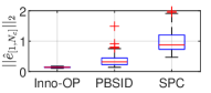
(a) SNR=$20$dB

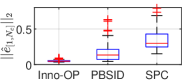
(b) SNR=$30$dB

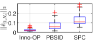
(c) SNR=$40$dB

Figure 1: Boxplots of one-step prediction errors at different SNRs in $100$ simulations.

Then we investigate the correctness of Theorem 4 based on a single Monte Carlo run with ${\rm SNR}=$30\text{\,}\mathrm{d}\mathrm{B}$$. We create two trajectories of innovation estimates by varying $\rho$ and implement the resultant data-driven OP in Algorithm 1. Specifically, using $\rho=23$ yields a stable matrix $\Theta_{1}$, whereas using $\rho=90$ yields an unstable matrix $\Theta_{2}$. In this way, there are two data-driven OPs developed and their one-step prediction errors are profiled in Fig. 2. Clearly, prediction errors induced by $\Theta_{1}$ show a bounded variance, while those induced by $\Theta_{2}$ diverge, thereby clearly verifying the statement in Theorem 4.

Figure 2: One-step prediction errors of data-driven OPs with $\Theta_{1}$ and $\Theta_{2}$ in a single Monte Carlo run.

3.2 Results of data-driven predictive control

In this subsection, we investigate the empirical closed-loop control performance of Inno-DeePC based on innovation estimates. For a comprehensive comparison, four different control strategies are implemented.

1. SSKF-MPC: The model-based control scheme with the SSKF-based OP (3), where $(A,B,C,D,K)$ is assumed to be known and the SSKF (2) is used for forward prediction. This can be viewed as the “oracle” control design based on perfectly known model dynamics and noise statistics.

2. Inno-DeePC: The proposed Inno-DeePC scheme (38) based on the data-driven OP in Algorithm 1, where $\hat{e}_{\rm p}(0)$ is initialized by solving (21) with $\hat{E}_{\rm p}$. Because of innovation estimation errors, it does not perform equally to SSKF-MPC.

3. SPC: The classical SPC scheme (37) [15].

4. Reg-DeePC: The regularized DeePC [13, Eq. (16)], where the regularization parameter $\lambda$ is optimally selected from a grid of values within $[10^{-2},10^{4}]$.

The system settings are identical to those in the previous subsection. In three data-driven control strategies, $L_{p}$ is selected as $30$. For predictive control design, we choose $Q=1$, $R=0.01$, $L_{f}=30$, the reference $r(k)=\mathrm{sin}(2\pi k/N_{c}),~{}k=1,2,...,N_{c}$ and the stage-wise constraints as $\mathbb{U}_{k}=\{u|-2\leq u\leq 2\}$ and $\mathbb{Y}_{k}=\{\hat{y}|-2\leq\hat{y}\leq 2\}$. All optimization problems are solved using the Gurobi package [18] via the YALMIP interface [29]. To evaluate the control performance, the indices $\{\mathcal{J}_{\rm total},\mathcal{J}_{y},\mathcal{J}_{u}\}$ are introduced:

$$\mathcal{J}_{\rm total}=\underbrace{\sum_{k=1}^{N_{c}}||y(k)-r(k)||_{Q}^{2}}_{\triangleq\mathcal{J}_{y}}+\underbrace{\sum_{k=1}^{N_{c}}||u(k)||_{R}^{2}}_{\triangleq\mathcal{J}_{u}},$$ (40)

where $u(k)$ is the control action decided by each control strategy and $y(k)$ denotes the realized system output.

The boxplots of $\mathcal{J}_{\rm total}$ in $100$ Monte Carlo simulations are shown in Fig. 3, and more detailed results of $\mathcal{J}_{u}$ and $\mathcal{J}_{y}$ are presented in Table 1. It can be seen that the Reg-DeePC strategy achieves better control performance than the generic SPC. Meanwhile, the proposed Inno-DeePC outperforms both SPC and Reg-DeePC under all settings, featuring a narrower gap with SSKF-MPC. In particular, the advantage of the Inno-DeePC scheme becomes more pronounced at lower SNR. This demonstrates that the proposed Inno-DeePC scheme draws strength from using innovations in improving the control performance of stochastic systems.

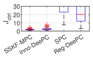
(a) SNR=$20$dB

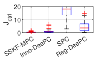
(b) SNR=$30$dB

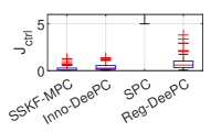
(c) SNR=$40$dB

Figure 3: Boxplots of $\mathcal{J}_{\rm total}$ at different SNRs in $100$ simulations.

Table 1: Statistics of $\mathcal{J}_{u}$ and $\mathcal{J}_{y}$ (Mean $\pm$ Standard Deviation) at Different SNRs in $100$ Monte Carlo Simulations

	SNR = 20dB		SNR = 30dB		SNR = 40dB
	$\mathcal{J}_{u}$	$\mathcal{J}_{y}$	$\mathcal{J}_{u}$	$\mathcal{J}_{y}$	$\mathcal{J}_{u}$	$\mathcal{J}_{y}$
SSKF-MPC	$1.09\pm 0.11$	$1.92\pm 0.58$	$0.81\pm 0.05$	$0.35\pm 0.25$	$0.78\pm 0.05$	$0.21\pm 0.24$
Inno-DeePC	$0.99\pm 0.17$	$2.61\pm 1.09$	$0.81\pm 0.13$	$0.87\pm 0.91$	$0.79\pm 0.09$	$0.39\pm 0.32$
SPC	$1.02\pm 0.83$	$63.70\pm 18.68$	$0.99\pm 0.44$	$24.83\pm 34.69$	$1.02\pm 0.17$	$16.35\pm 5.38$
Reg-DeePC	$0.44\pm 0.46$	$27.03\pm 9.75$	$0.69\pm 0.23$	$6.19\pm 8.67$	$0.78\pm 0.10$	$5.53\pm 2.30$

4 Concluding Remarks

In this paper, we proposed a new data-driven approach to output prediction and control problems of stochastic LTI systems. By utilizing the innovation form of stochastic systems, all additive uncertainty is recaptured in terms of innovations that can be readily estimated from input-output data without knowing system matrices. By applying the generic fundamental lemma to the innovation form, we derived an innovation-based data-driven OP that bypasses the model identification and state estimation. The equivalence between the data-driven OP and the SSKF-based OP was established under certain conditions, which inspires an easy closed-loop implementation of the data-driven OP. We established the sufficient condition for the boundedness of the second moment of prediction errors, which yields a practical guideline to verify the “validity” of innovation estimates and the induced data-driven OP. The usage of the proposed data-driven OP in control design gives rise to a new DeePC formulation called Inno-DeePC. Numerical case studies showed the performance improvement of the proposed methods based on innovation estimates over existing formulations. In future work, a meaningful direction is to extend Inno-DeePC to the stochastic predictive control scheme, e.g. chance-constrained control, to handle the uncertainty of output prediction.

Appendix: Data-Driven Innovation Estimation

Due to the Schur stability of $\bar{A}=A-KC$, $\bar{A}^{\rho}\approx 0$ holds approximately for a sufficiently large $\rho\geq 0$. Thus, the VARX model can be expressed in matrix form as [11]:

$$\mathcal{H}_{1}(y_{[1:N]})\approx ~{}\Phi_{y}\mathcal{H}_{\rho}(y_{[1-\rho:N-1]})+\Phi_{u}\mathcal{H}_{\rho}(u_{[1-\rho:N-1]})$$ (41)

$$~{}+D\mathcal{H}_{1}(u_{[1:N]})+\mathcal{H}_{1}(e_{[1:N]}),$$

where $\Phi_{y}\triangleq C\Delta_{\rho}^{y}$ and $\Phi_{u}\triangleq C\Delta_{\rho}^{u}$ are matrices encompassing MPs of the innovation form (4) with $\bar{B}\triangleq B-KD$ and

$$\Delta_{\rho}^{y}=\begin{bmatrix}\bar{A}^{\rho-1}K&\cdots&\bar{A}K&K\end{bmatrix},~{}\Delta_{\rho}^{u}=\begin{bmatrix}\bar{A}^{\rho-1}\bar{B}&\cdots&\bar{A}\bar{B}&\bar{B}\end{bmatrix}.$$ (42)

To estimate MPs $\{\Phi_{y},\Phi_{u}\}$ and $D$, one can resolve the following least-squares regression (LSR) problem [35]:

$$\min_{\Phi_{y},\Phi_{u},D}\left\|\mathcal{H}_{1}(y_{[1:N]})-\begin{bmatrix}\Phi_{y}~{}\Phi_{u}~{}D\end{bmatrix}\begin{bmatrix}\mathcal{H}_{\rho}(y_{[1-\rho:N-1]})\\ \mathcal{H}_{\rho}(u_{[1-\rho:N-1]})\\ \mathcal{H}_{1}(u_{[1:N]})\end{bmatrix}\right\|_{F}^{2},$$ (43)

where additional input-output data $\{u(i),y(i)\}_{i=1-\rho}^{0}$ preceding $\{u(i),y(i)\}_{i=1}^{N}$ is required. It is noted that the residuals of (43) provide an explicit approximation of $\mathcal{H}_{1}(e_{[1:N]})$, based on which $\hat{E}_{d}$ can be constructed [32]. We also mention that $\rho$ shall be suitably chosen to achieve a desirable trade-off. Specifically, a large $\rho>n$ is typically needed in LSR to reduce approximation errors caused by $\bar{A}^{\rho}$, but choosing $\rho$ larger than necessary leads to a large variance of estimation, which is essentially an overfitting phenomenon [11].

References

- [1] Daniele Alpago, Florian Dörfler, and John Lygeros. An extended kalman filter for data-enabled predictive control. IEEE Control Systems Letters, 4(4):994–999, 2020.
- [2] Karl Johan Åström and Peter Eykhoff. System identification—a survey. Automatica, 7(2):123–162, 1971.
- [3] Giacomo Baggio, Danielle S Bassett, and Fabio Pasqualetti. Data-driven control of complex networks. Nature Communications, 12(1):1–13, 2021.
- [4] Julian Berberich, Johannes Köhler, Matthias A Müller, and Frank Allgöwer. Data-driven model predictive control with stability and robustness guarantees. IEEE Transactions on Automatic Control, 66(4):1702–1717, 2021.
- [5] Deborah Bilgic, Alexander Koch, Guanru Pan, and Timm Faulwasser. Toward data-driven predictive control of multi-energy distribution systems. Electric Power Systems Research, 212:108311, 2022.
- [6] Joscha Bongard, Julian Berberich, Johannes Köhler, and Frank Allgower. Robust stability analysis of a simple data-driven model predictive control approach. IEEE Transactions on Automatic Control, 2022.
- [7] V Breschi, T Bou Hamdan, Guillaume Mercère, and S Formentin. Tuning of subspace predictive controls. IFAC-PapersOnLine, 56(3):103–108, 2023.
- [8] Valentina Breschi, Alessandro Chiuso, and Simone Formentin. Data-driven predictive control in a stochastic setting: a unified framework. Automatica, 152:110961, 2023.
- [9] Paolo Gherardo Carlet, Andrea Favato, Saverio Bolognani, and Florian Dörfler. Data-driven continuous-set predictive current control for synchronous motor drives. IEEE Transactions on Power Electronics, 37(6):6637–6646, 2022.
- [10] Venkatesh Chinde, Yashen Lin, and Matthew J Ellis. Data-enabled predictive control for building HVAC systems. Journal of Dynamic Systems, Measurement, and Control, 144(8):081001, 2022.
- [11] Alessandro Chiuso. The role of vector autoregressive modeling in predictor-based subspace identification. Automatica, 43(6):1034–1048, 2007.
- [12] Jeremy Coulson, John Lygeros, and Florian Dörfler. Data-enabled predictive control: In the shallows of the DeePC. In 2019 18th European Control Conference (ECC), pages 307–312. IEEE, 2019.
- [13] Florian Dörfler, Jeremy Coulson, and Ivan Markovsky. Bridging direct & indirect data-driven control formulations via regularizations and relaxations. IEEE Transactions on Automatic Control, 2022.
- [14] Ezzat Elokda, Jeremy Coulson, Paul N Beuchat, John Lygeros, and Florian Dörfler. Data-enabled predictive control for quadcopters. International Journal of Robust and Nonlinear Control, 31(18):8916–8936, 2021.
- [15] Wouter Favoreel, Bart De Moor, and Michel Gevers. SPC: Subspace predictive control. IFAC Proceedings Volumes, 32(2):4004–4009, 1999.
- [16] Randall T Fawcett, Kereshmeh Afsari, Aaron D Ames, and Kaveh Akbari Hamed. Toward a data-driven template model for quadrupedal locomotion. IEEE Robotics and Automation Letters, 7(3):7636–7643, 2022.
- [17] Michel Gevers. Identification for control: From the early achievements to the revival of experiment design. European Journal of Control, 11(4-5):335–352, 2005.
- [18] Gurobi Optimization, LLC. Gurobi Optimizer Reference Manual, 2023.
- [19] Håkan Hjalmarsson. From experiment design to closed-loop control. Automatica, 41(3):393–438, 2005.
- [20] Zhong-Sheng Hou and Zhuo Wang. From model-based control to data-driven control: Survey, classification and perspective. Information Sciences, 235:3–35, 2013.
- [21] Ivo Houtzager, Jan-Willem van Wingerden, and Michel Verhaegen. Varmax-based closed-loop subspace model identification. In Proceedings of the 48h IEEE Conference on Decision and Control (CDC) held jointly with 2009 28th Chinese Control Conference, pages 3370–3375. IEEE, 2009.
- [22] Biao Huang and Ramesh Kadali. Dynamic Modeling, Predictive Control and Performance Monitoring: A Data-Driven Subspace Approach. Springer, 2008.
- [23] Linbin Huang, Jeremy Coulson, John Lygeros, and Florian Dörfler. Decentralized data-enabled predictive control for power system oscillation damping. IEEE Transactions on Control Systems Technology, 30(3):1065–1077, 2021.
- [24] Linbin Huang, Jianzhe Zhen, John Lygeros, and Florian Dörfler. Quadratic regularization of data-enabled predictive control: Theory and application to power converter experiments. IFAC-PapersOnLine, 54(7):192–197, 2021.
- [25] Linbin Huang, Jianzhe Zhen, John Lygeros, and Florian Dörfler. Robust data-enabled predictive control: Tractable formulations and performance guarantees. IEEE Transactions on Automatic Control, 2023.
- [26] Edward W Kamen and Jonathan K Su. Introduction to optimal estimation. Springer Science & Business Media, 1999.
- [27] S Kerz, J Teutsch, T Brüdigam, D Wollherr, and M Leibold. Data-driven tube-based stochastic predictive control. arXiv preprint arXiv:2112.04439, 2023.
- [28] Xiyao Liu, Haitao Chang, Zhenyu Lu, and Panfeng Huang. Data-driven moving horizon estimation for angular velocity of space noncooperative target in eddy current de-tumbling mission. arXiv preprint arXiv:2301.05351, 2023.
- [29] J. Löfberg. YALMIP: A toolbox for modeling and optimization in MATLAB. In 2004 IEEE International Conference on Robotics and Automation, pages 284–289, 2004.
- [30] Ivan Markovsky and Florian Dörfler. Behavioral systems theory in data-driven analysis, signal processing, and control. Annual Reviews in Control, 52:42–64, 2021.
- [31] Ivan Markovsky and Florian Dörfler. Data-driven dynamic interpolation and approximation. Automatica, 135:110008, 2022.
- [32] Guillaume Mercère, Ivan Markovsky, and José A Ramos. Innovation-based subspace identification in open-and closed-loop. In 2016 IEEE 55th Conference on Decision and Control (CDC), pages 2951–2956. IEEE, 2016.
- [33] Guanru Pan, Ruchuan Ou, and Timm Faulwasser. On a stochastic fundamental lemma and its use for data-driven optimal control. IEEE Transactions on Automatic Control, 68(10):5922–5937, 2022.
- [34] Guanru Pan, Ruchuan Ou, and Timm Faulwasser. On data-driven stochastic output-feedback predictive control. arXiv preprint arXiv:2211.17074, 2022.
- [35] Gijs Van der Veen, Jan-Willem van Wingerden, Marco Bergamasco, Marco Lovera, and Michel Verhaegen. Closed-loop subspace identification methods: An overview. IET Control Theory & Applications, 7(10):1339–1358, 2013.
- [36] Henk J van Waarde, Claudio De Persis, M Kanat Camlibel, and Pietro Tesi. Willems’ fundamental lemma for state-space systems and its extension to multiple datasets. IEEE Control Systems Letters, 4(3):602–607, 2020.
- [37] Jan C Willems and Jan W Polderman. Introduction to Mathematical Systems Theory: A Behavioral Approach, volume 26. Springer Science & Business Media, 1997.
- [38] Jan C Willems, Paolo Rapisarda, Ivan Markovsky, and Bart LM De Moor. A note on persistency of excitation. Systems & Control Letters, 54(4):325–329, 2005.
- [39] Tobias M Wolff, Victor G Lopez, and Matthias A Müller. Robust data-driven moving horizon estimation for linear discrete-time systems. arXiv preprint arXiv:2210.09017, 2022.