Interface dynamics in the two-dimensional quantum Ising model
Abstract
In a recent letter [Phys. Rev. Lett. 129, 120601 (2022)] we have shown that the dynamics of interfaces, in the symmetry-broken phase of the two-dimensional ferromagnetic quantum Ising model, displays a robust form of ergodicity breaking. In this paper, we elaborate more on the issue. First, we discuss two classes of initial states on the square lattice, the dynamics of which is driven by complementary terms in the effective Hamiltonian and may be solved exactly: (a) strips of consecutive neighbouring spins aligned in the opposite direction of the surrounding spins, and (b) a large class of initial states, characterized by the presence of a well-defined “smooth” interface separating two infinitely extended regions with oppositely aligned spins. The evolution of the latter states can be mapped onto that of an effective one-dimensional fermionic chain, which is integrable in the infinite-coupling limit. In this case, deep connections with noteworthy results in mathematics emerge, as well as with similar problems in classical statistical physics. We present a detailed analysis of the evolution of these interfaces both on the lattice and in a suitable continuum limit, including the interface fluctuations and the dynamics of entanglement entropy. Second, we provide analytical and numerical evidence supporting the conclusion that the observed non-ergodicity—arising from Stark localization of the effective fermionic excitations—persists away from the infinite-Ising-coupling limit, and we highlight the presence of a timescale for the decay of a region of large linear size . The implications of our work for the classic problem of the decay of a false vacuum are also discussed.
I Introduction
The dynamical nucleation of a region of true vacuum in a sea of false vacuum is a classic problem in statistical mechanics [1, 2, 3]. Most of the progress, however, has been achieved in the context of stochastic dynamics so far, since the unitary quantum dynamics constitutes a significant challenge. Stochastic dynamics often provides an adequate description of equilibrium condensed matter systems, such as magnets or crystal-liquid mixtures, due to the continuous influence of noisy environmental degrees of freedom, which act like a bath at a well-defined temperature. Nevertheless, there are situations in which one cannot neglect the unitary nature of the quantum dynamical evolution from a pure initial state. This is the case, for instance, in a cosmological setting: the problem was studied long ago by Kobzarev, Okun and Voloshin [4], and then by Coleman and Callan [5, 6, 7], finding also applications in inflationary models of the universe [8]. In addition, unitary evolution plays a crucial role in recent experiments with ultracold matter, which make it possible to investigate analoguous false-vacuum-decay phenomena in coherent quantum many-body systems, where the nucleation is driven by quantum rather than thermal fluctuations (see, e.g. Ref. [9] for a recent experiment in this direction). Finally, there are quantum optimization algorithms [10, 11, 12], which are designed to find the ground state of a classical Ising model (a computationally NP-hard task), but can incur in several dynamical drawbacks associated to classical or quantum effects [13, 14, 15]. One can only expect that, in the near future, quantum simulators will allow finely controlled explorations of this physics using table-top experiments, allowing the observation of more counter-intuitive effects of coherent quantum dynamics.
With these motivations in mind, and following Ref. [16], here we set to study the unitary evolution of nucleated vacuum bubbles in the two-dimensional () ferromagnetic quantum Ising model with longitudinal and transverse fields of strengths and , respectively. These vacuum bubbles correspond, to a first approximation, to regions on the lattice with a certain spin orientation, surrounded by a sea of spins with opposite orientation. We find that the limit of large Ising coupling , is amenable to several simplifications: this is due to the emergence of a constraint on the length of the interface, which separates the regions of opposite spin alignment in the initial state.
In this context, we address the issue of Hilbert space fragmentation, recently investigated in Refs. [17, 18], and elaborate on the effective Hamiltonian governing the dynamics. Such effective Hamiltonian further simplifies, and becomes amenable of analytical treatment, when restricted to two classes of initial states. The first is defined by the presence of a strip of aligned consecutive spins, running along one of the principal axes of the square lattice; the second, by an infinitely long “smooth” interface separating regions with oppositely aligned spins. The dynamics of the latter can be mapped onto a one-dimensional chain of fermions, which becomes integrable for . The integrability of this effective model is responsible for ergodicity breaking: we will show, for example, that the corner of a large bubble melts and reconstructs itself periodically in time, with period . The same periodic dynamics generically characterizes an initially smooth profile, the evolution of which turns out to take a particularly simple form in a suitable continuum limit, which we discuss in detail. The proposed mapping on the fermionic chain allows us to study also interface fluctuations and the evolution of the entanglement entropy for an infinitely extended right-angled corner. In addition, we will also unveil surprising connections with classic mathematical results, concerning the limiting shape of random Young diagrams, as well as with similar problems in classical statistical physics.
Based on the mapping, we can trace back the observed ergodicity breaking in the dynamics of the interface in to the Wannier-Stark localization of the single-particle eigenstates of the dual fermionic theory. Surprisingly, we find that, even moving away from the limit in a perturbation theory in , the emerging many-particle eigenstates of the resulting perturbative Hamiltonian are Stark many-body localized (MBL) [19, 20]: thus, they display the typical MBL phenomenology [21, 22, 23, 24, 25], which carries over to the quantum Ising model. As several works have questioned the existence of MBL in more than one spatial dimension [26, 27] (even in the disordered version of the model studied here [28]), the present case provides a valuable example of a mechanism by which the non-ergodic dynamics of a one-dimensional model renders the dynamics of the dual two-dimensional model non-ergodic. Moreover, the phenomenology observed here reminds of the confinement that takes place in [29, 30].
It is interesting to remark also that the quantum Ising model displays strong stability of magnetic domains even when, in the absence of external fields, a Floquet dynamics is considered, characterized by imperfect stroboscopic single-spin kicks [31]. Therefore, the interest in this model is renewed also by the possibility of probing different mechanisms for the breakdown of ergodicity, even if disorder-induced MBL is not present.
The discussion of the dynamics of an infinitely extended smooth interface (separating two semi-infinite domains) can be used as a starting point to investigate the case of finite but large “bubbles” of one phase, surrounded by the other. In truth, this was the original motivation of the work, being it related to the problem of the decay of a false vacuum. In particular, we discuss and estimate the relevant timescales which are involved in the possible “melting” of the bubble, the complete description of which is however beyond the scope of the present work.
The rest of the presentation is organized as follows. In Sec. II we briefly introduce the Ising model, discussing how it reduces to a so-called “PXP” model in the limit of strong coupling (Sec. II.1), for which Hilbert space fragmentation is expected to occur (Sec. II.2). In Sec. III we focus on the dynamics of the model in the infinite-coupling limit. In particular, in Sec. III.1 we study strip-like initial configurations, while in Sec. III.2 we consider more generic initial states, characterized by the presence of a smooth and infinite interface separating spins with opposite orientation. In Sec. III.3 we describe the continuum limit of the latter, and the connections with a semiclassical limit for the single-particle dynamics. In Sec. IV we focus on a subset of initial configurations belonging to the general class discussed in Sec. III.2, i.e. a corner-shaped interface: in Sec. IV.1 we determine the average shape of such interface during the dynamics, while in Sec. IV.2 we study its fluctuations. In Sec. IV.3 we focus on the time evolution of the entanglement, discussing the computation of the entanglement entropy. In Sec. IV.4 we show the connection between the unitary dynamics of the interface of a corner and some known results concerning the phenomenon of Plancherel measure concentration in random Young diagrams. Moving to Sec. V, we discuss how the emergent integrability can be broken, either in a domain of finite size (Sec. V.1) or when the ferromagnetic coupling is no longer assumed to be infinitely large (Sec. V.2 and V.3), giving also a comparison between the lattice and the field theoretic dynamics of false vacuum bubbles (Sec. V.4). Finally, in Sec. VI we present our conclusions and outlook.
Part of the work presented here was briefly reported in Ref. [16].
II The Model
As anticipated in the Introduction, we are interested in the dynamics of the quantum Ising model on a two-dimensional square lattice. The Hamiltonian reads
| (1) |
where are Pauli matrices acting on a lattice site , indicates the restriction of the sum to nearest neighbors, and are the strength of the transverse and longitudinal magnetic fields, respectively, and is the ferromagnetic coupling. We set , while we let take both positive and negative values: the sign of , indeed, will be relevant in Sec. V.2.
In thermal equilibrium at temperature , this model displays a quantum phase transition at and , belonging to the universality class of the classical 3 Ising model: upon decreasing below a critical value , it passes from a quantum paramagnet to a quantum ferromagnet, characterized by two degenerate, magnetized ground states spontaneously breaking the symmetry. Upon increasing , the ferromagnetic phase survives up to a finite critical temperature (depending on and ), since the energetic cost of creating domains with reversed magnetization increases upon increasing their perimeter (as entailed by Peierls’ argument). At , the model becomes the classical Ising model, therefore displaying the corresponding critical properties. These critical properties also characterize the transition occurring on the line of thermal critical points, which joins the classical model at to the quantum critical point at . The longitudinal field breaks explicitly the symmetry of the two possible ground states, lifting their degeneracy. Accordingly, the model at and undergoes a first-order quantum phase transition as crosses . As discussed in the Introduction, one expects that highly non-equilibrium false vacuum states exhibit a slow decay, through the nucleation of bubbles of characteristic size related to the inverse decay rate. With this background motivation in mind, below we will be interested in the fate of such bubbles, and more generally of interfaces, under the subsequent, coherent unitary evolution.
Studying the dynamics of interacting models constitutes a priori a formidable task: numerical methods are limited to very small system sizes or very short times. In addition, analytical tools are restricted to near-equilibrium conditions, or generally involve uncontrolled approximations, as dynamical mean-field theory [32] or kinetic equations [33]. Despite these shortcomings, insight can be obtained from suitable limits. While the extreme paramagnetic regime reduces to a set of weakly interacting “magnonic” excitations, the strongly-coupled ferromagnetic regime retains great part of the interacting nature of the problem. It is the purpose of this work to show that, in such strong-coupling limit, there exists a relevant class of highly excited, non-thermal initial states, the dynamics of which is amenable of analytical treatment. In particular, in the next Sections we show that the formal limit of infinitely strong ferromagnetic coupling actually renders a highly non-trivial constrained dynamical problem, characterized by a fragmented Hilbert space.
II.1 Constrained dynamics in the strong-coupling limit
Starting from this Section, and throughout this work, we will consider the strong-coupling limit . In practice, we start by formally taking , while later on in Sec. V.2 we will relax this assumption. In this limit it is particularly convenient to study the problem in the basis of the eigenstates of at each lattice site , with and . At the leading order in , the model is actually diagonal (i.e., classical) in this basis and, up to a constant, the energy of each of these eigenstates is given by , where is the number of distinct pairs of neighbouring spins with opposite orientation. Accordingly, the Hilbert space at infinite coupling is fragmented into dynamically independent sectors with , each sector being identified by [17, 16]. Being , in fact, no transitions are actually allowed from a state in to one in , unless , since the energy difference between them would be infinite. Note that, equivalently, measures the total length of the domain walls which are present on the lattice, separating the regions with spins from those with . Accordingly, in the limit , dynamical constraints emerge, in the form of a perimeter constraint on the bubbles of spins aligned along the same direction. Stated more formally, the domain-wall length operator
| (2) |
is exactly conserved by in the limit.
As a consequence of the perimeter constraint, the dynamics of the model can be effectively studied by focusing on each sector separately, thereby reducing significantly the complexity of the problem. Let us start by determining the reduced Hamiltonian in by elementary reasoning. Since the total domain-wall length must be conserved, the only spins that can be flipped by the term in Eq. (1) are those that just displace an existing domain wall. In practice, these spins are characterized by having two neighbours up () and two neighbours down (), such that their flipping does not change the number of distinct pairs of neighbouring spins with opposite orientation, i.e., the length of the domain wall in the associated plaquettes. Considering the possible configurations of the four spins which satisfy this constraint and are, respectively, left/right/above/below a site with a certain spin orientation, one easily gets convinced that the only allowed transitions are those generated by the following reduced Hamiltonian:
| (3) |
where we introduced the projectors
| (4) |
The term in Eq. (1), being diagonal in , is instead unaffected. One can recognize that Eq. (3) has the structure of a so-called PXP Hamiltonian [34].
The elementary procedure outlined above can be viewed as the first step of a systematic elimination, from a Hamiltonian with large energy gaps, of highly non-resonant transitions. This is formally implemented by an order-by-order unitary transformation known as Schrieffer-Wolff transformation [35]. In Sec. V.2 we will be concerned with the possible additional contributions to Eq. (3) due to higher-order corrections .
We stress here that the constrained Hamiltonian in Eq. (3) is actually similar to the one describing strongly interacting Rydberg atom arrays [36, 37]. In this case, each spin- describes a trapped neutral atom, which can be in either its ground state () or in a highly excited Rydberg state (). The basic model Hamiltonian that describes a lattice of such strongly interacting atoms reads [36]
| (5) |
where counts the local number of atoms excited to the Rydberg state while the interaction is very strong for neighboring sites and it decays rapidly as the distance increases. Upon rearranging the various terms, Eq. (5) may be viewed as a quantum Ising model; the strong coupling , however, couples here to the operator rather than to . When this nearest-neighbor interaction becomes larger than all the other energy scales— as it happens in the so-called regime of Rydberg blockade—its dynamics is described by an effective constrained Hamiltonian,
| (6) |
which is obtained from Eq. (5) by setting for neighboring atoms and otherwise. In this case, pairs of neighboring excited atoms are completely frozen, and an atom can flip only if all its four neighbors are in the ground state, which is expressed by the last term in Eq. (6). The Hamiltonian in Eq. (3), instead, imposes a different form of the constraint, which implements the local perimeter-conserving motion of domain walls. It is interesting to note, however, that the two constraints differ only by a strong longitudinal field term, which can be adjusted to transform one into the other. Specifically, by identifying , it is sufficient to take a single-atom energy level detuning to obtain the Ising model (1) and hence, in the regime of Rydberg-blockade, the effective Hamiltonian in Eq. (3) 111We note, however, that this might be problematic at experimental level, as the Rydberg interactions are very sensitive to the precise position of the trapped atoms, resulting in unwanted noisy fluctuations of the longitudinal field. We thank Hannes Pichler for this clarification (private communication)..
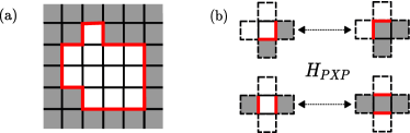
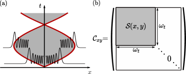
The Hamiltonian in Eq. (3) can be alternatively written via a shorthand notation, which describes graphically the transitions induced on the part of domain wall (in red) existing in the square plaquette surrounding a spin (i.e. the dual lattice), due to its allowed flipping (see also Fig. 1):
| (7) |
Here, the transitions due to the coupling are apparent: either a domain wall corner is moved across the diagonal of a plaquette ( or ), or two parallel segments of the domain wall are recombined across opposite sides of the plaquette (). These moves guarantee the conservation of the domain wall length.
II.2 Hilbert space fragmentation
The convenient notation of Eq. (7) makes it possible to analyze the fate of the dynamics of large portions of the lattice in various cases. For instance, consider multiple, distant spins oriented up, i.e. with , embedded in a sea of oppositely aligned spins, with . This configuration is fully frozen, as no allowed transition can shift any of the domain walls. Thus, all of these states are eigenstates of the constrained Hamiltonian (7). This simple example—easily generalizable to many others [17]—shows that individual sectors are, in general, further heavily fragmented. More formally, one can introduce the notion of Krylov subspace of a state : by definition, it is the subspace of spanned by the set of vectors , where is the Hamiltonian of the system. With this definition, one recognizes that the Krylov sector of a state may not coincide with the full , but instead represent a finer shattering. A detailed study of the Krylov sectors of the model under consideration was presented in Ref. [18]; in this work, instead, we will be concerned mainly with the dynamical effects of the fragmentation on some physically relevant states. This is what we set out to study in the next Section.
III Infinite-coupling dynamics for strips and smooth domain walls
In the previous Section we have argued that, in the limit of large , the dynamics of the quantum Ising model simplifies significantly, because of the presence of emergent constraints. Here, we show that this simplification is really substantial in some particular cases, as it leads to simple one-dimensional effective models.
From Eq. (7), one can see that the first two terms ( and ) correspond to the translation of a domain wall, while the last one () cuts two nearby portions of domain wall into two halves and recombines those belonging to different portions. If the initial condition has a geometry that allows only one of the two types of transitions, then it is possible to gain further analytical control on the dynamics. In particular, we show in Sec. III.1 that initial conditions consisting of a thin, pseudo-1 domain are only affected by interface-recombining moves. This allows us to make a connection with 1 PXP and confining Ising models. In Sec. III.2, instead, we show that if the lattice is cut by a single, Lipschitz-continuous interface (this notion will be clarified further below), then its dynamics can be studied via an effective 1 model of non-interacting fermions in a linear potential. Its emergent integrability allows us to predict the evolution exactly, and to describe precisely how ergodicity is broken.
III.1 Strip-like configurations
In this Section, we consider a class of initial configurations that are essentially one-dimensional. As it was also pointed out in Ref. [17], for this type of states it is possible to establish an explicit connection with PXP models. We show here that, when the initial configuration has no overlap with scarred states 222Quantum many body scars denote special eigenstates of the spectrum that does not satisfy the eigenstate thermalization hypothesis. This means that the expectation values of observables evaluated on such states does not attain the thermal value, even if their energy density corresponds to infinite temperature states., it is possible to calculate the asymptotic magnetization of the bubble.
We focus on an initial condition consisting of a linear strip of consecutive down spins (), along one of the principal lattice axes, surrounded by up spins (). In the Krylov sector of this configuration (see Sec. II.2 above), and in the absence of longitudinal magnetic field (i.e. for ), the PXP Hamiltonian (3) reduces to the one-dimensional PXP Hamiltonian familiar from tilted bosonic traps [40], one-dimensional Rydberg-blockaded arrays [41], or dimer models [42]. Indeed, due to the perimeter constraint, neither the spins outside the initial strip nor those at its two ends can be flipped by ; accordingly, the only dynamical degrees of freedom are the internal spins initially set to be down. This reduces the full, dynamics to an effectively 1 dynamics.
For convenience, we label the accessible basis states by the corresponding 1 configuration of the spins in the strip; the initial state is therefore denoted by . Assuming for the moment , the Hamiltonian (3) reduces to
| (8) |
as the spins above and below the strip are fixed to be up. Above, we are also taking into account that the first and last spin of the strip cannot be flipped.
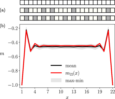
Because of the constraints, not all 1 configurations are dynamically accessible: for example, those containing two or more consecutive spins up are not. This implies that the spins adjacent to a spin up are down, and that completely fragmented configurations consist of singlets or pairs of spins down, separated by single spins up, see Fig. 2a. Denoting by the number of spins which are reversed compared to the initial configuration, the number of accessible basis states in the strip of length satisfies the recursion relation (see also App. A)
| (9) |
which has solution
| (10) |
once the initial condition for all is enforced. The maximum number of spins that can be flipped satisfying the perimeter constraint is
| (11) |
and the total number of accessible configurations is therefore given by
| (12) |
i.e. by the -th Fibonacci number [43].
It is worth recalling that PXP Hamiltonians exhibit quantum many-body scars [34], i.e. particular eigenstates that violate the eigenstate thermalization hypothesis [44, 45]. The number of such eigenstates increases only algebraically upon increasing the system size, making them very rare in the many-body spectrum. However, they profoundly affect the dynamical properties of particular initial configurations: for instance, the Néel state exhibits remarkable long-lived revivals, as discovered in early experimental explorations [46]. While it has become clear that these non-thermal eigenstates slowly disappear in the large-size limit of the PXP model, their ultimate origin is presently unclear, despite significant research efforts, and is the subject of an active ongoing debate [47]. On the other hand, the initial state we consider here is not significantly affected by quantum many-body scars [34, 47]. Accordingly, it is expected that the magnetization profile along the chain at long times is compatible with an assumption of ergodicity, i.e. that all allowed configurations (having the same expectation value of the energy) will be occupied with uniform probability. Under this assumption, the long-time average magnetization at position along the strip of length is expected to be given by
| (13) |
as detailed in App. A. The explicit expression of the Fibonacci numbers [43],
| (14) |
in terms of the golden ratio , allows us to determine the resulting magnetization profile . We compare it with numerical simulations for short strips in Fig. 2, showing fairly good agreement with the assumption of ergodicity. The magnetization, as expected, is fixed at the boundaries of the strip, due to the fact that fluctuations cannot occur there, while its absolute values decreases upon moving away from the boundaries. In particular, the value of the magnetization in the middle of an infinitely long strip can be easily obtained by taking first the limit and then in Eq. (13), finding (see App. A)
| (15) |
where we used Eq. (14). The (alternating-sign) approach of to upon increasing turns out to be exponential, with a rather short characteristic length . The derivation of this fact is provided again in App. A, see Eq. (88).
The solution presented above applies to the case of a single strip of reversed spins running along one of the principle lattice axes. In the presence of more than one strip (possibly having different orientations), the same results apply to each strip separately as long as the spins belonging to two different strips do not have a common nearest-neighbour. In fact, in case they have one, a change of its orientation might cause the interfaces of the two strips to merge and, due to the resulting shape, the term in the effective Hamiltonian (7) would contribute to the dynamics as well. In particular, it is easy to realize that the initial condition discussed above is dynamically connected with the configuration consisting of the largest rectangular “envelope”, which contains all initial strips with at least one common nearest-neighbour. While the dynamics in this case turns out to be highly non-trivial, in Sec. IV we will focus on what happens to one of the corners of this rectangular envelope when it is sufficiently extended.
We conclude this Section by noting that what we have done, essentially, was to compute local observables in the infinite-temperature ensemble within the Krylov sector of the initial configuration , instead of computing the expectation values on . The two procedures are equivalent, since the initial state lies in the middle of the spectrum (and thus is an infinite-temperature state) 333That lies in the middle of the spectrum follows from the fact that, first, it holds ; and second, that the spectrum is symmetric around zero ( commutes with the space reflection operator , and anti-commutes with the spectral reflection operator [127])., and the 1 PXP model is ergodic [34, 47].
III.2 Smooth domain walls on the lattice
In the previous Section we considered strip-like initial configurations, the dynamics of which involved only the operators of Eq. (7), i.e. only domain-wall-breaking transitions. We now turn to a different family of initial states for which, instead, the only involved operators are or : thus, solely domain-wall-moving transitions are generated.
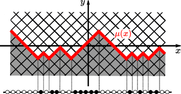
For later convenience, let us rotate by a angle with respect to the vertical and horizontal directions the square lattice on which the model is defined, such that the lattice axes are oriented along the diagonals of the quadrants of the standard coordinate system, as shown in Fig. 3. Then, let us consider an interface separating a domain of spins up () from one of spins down (), highlighted in red in Fig. 3. We require that such an interface varies only slowly, so that it can be thought of as the graph of a function in the rotated frame, see Fig. 3. More precisely, the interface profile should be described by a quantum superposition of functions which are Lipschitz-continuous on the lattice, i.e.
| (16) |
Let us remark that, since only the operators or of the Hamiltonian in Eq. (7) act on these configurations, the Krylov sector of a Lipschitz state contains only Lipschitz states. Accordingly, the unitary dynamics starting from such configurations involves only Lipschitz states and their superpositions, and cannot generate kinks or overhangs of the interface. Two-dimensional initial states of this type, other than being rather generic in the context of interface dynamics, are interesting because they can be alternatively described as states of a corresponding one-dimensional system. The mapping simply consists in associating to each downward segment of the interface an empty site on the chain, and to each upward segment a site occupied by a particle (see Fig. 3), following the interface line from left to right. In practice, this mapping amounts at a differentiation: in fact, one associates an empty (resp. occupied) site if the domain-wall derivative is negative (resp. positive). As a consequence, the interface profile can be reconstructed by “integrating” the density profile on the chain [49, 50, 51, 52]:
| (17) |
The mapping described above works also in a classical setting, where a fluctuating interface induces on the 1 particles an effective dynamics, as the simple exclusion processes [53, 54, 55] (more on this at the beginning of Sec. IV). In the quantum setting, the statistics of the particles plays a fundamental role. For the case under consideration—i.e. the quantum Ising model—these particles have to be hard-core bosons, because at most one particle can be present at a lattice site, and those at different sites commute. Applying a Jordan-Wigner transformation, these hard-core bosons can be equivalently represented as fermions. From now on we will adopt this more convenient representation.
Having set up the mapping between the accessible basis states of the two systems, we can proceed to determine the 1 Hamiltonian on the chain, corresponding to the PXP Hamiltonian (7). With a bit of reasoning, one notices that each allowed spin flip in (which induces one of the transitions in the interface of Fig. 3) corresponds to a fermion hop along the chain. At the same time, in the presence of the longitudinal magnetic field , each spin flip in contributes with a energy difference depending on the corresponding upward/downward direction of the domain-wall transition , and therefore every fermion hop must be accompanied by the same energy change. This is achieved by introducing a linear potential in the Hamiltonian such that a particle jumping to the right (resp. left) gains (resp. loses) an energy . The same procedure applied to off-diagonal elements fixes the hopping term of the chain, leading to the fermionic Hamiltonian
| (18) |
defined up to a constant related to the choice of the origin of .
Equation (18) is the well-known Wannier-Stark Hamiltonian [56]. It is diagonalized by the unitary transformation
| (19) |
where and is the Bessel function of the first kind, yielding
| (20) |
The energy spectrum is thus given by a set of equally spaced levels , insensitive to . We anticipate that this feature will be important in the discussion about non-ergodicity, further below in Secs. V.2–V.3.
In terms of the functions introduced above we are now able to predict the dynamics of any Lipschitz initial state . In fact, such a state can be expressed as
| (21) |
on the chain, where the sequence contains the sites occupied at and is the vacuum of the chain. The time evolution of the operators is simply given by , and thus
| (22) | ||||
where we introduced
| (23) |
and used the completeness relation of the Bessel functions, Eq. (96). Similarly, by using the previous expression and by calculating some Wick contractions, one can determine the evolution of the average of the density , i.e.
| (24) | |||||
where we used the property in Eq. (92), and defined the averages over the initial state
| (25) |
As discussed above, corresponds to the average slope of the quantum-fluctuating interface in the original system, and therefore describes its evolution 444It is interesting to note that, by time-reversal symmetry, Eq. (24) can also be interpreted as the total probability of finding a single particle starting at at time , in the subset of positions at time .. Moreover, the expression for in Eq. (24) clearly shows that the dynamics in the cases and are simply connected by the minimal substitution (and that the latter, in particular, is independent of the sign of ).
Equation (24), and its dependence on time via (Eq. (23)), imply that the dynamics on the chain—and therefore the full dynamics—is periodic with period : this is due to the Bloch oscillations [56], which localize each fermion near its initial position . In fact, in Eq. (24) decays exponentially fast upon increasing beyond , and therefore each fermion, during the evolution, explores a region of space of amplitude (in units of the lattice spacing)
| (26) |
This perfect localization is a feature of the limit, and of the presence of a nonzero longitudinal field which makes a periodic function of time. If, instead, , one finds that . Accordingly, the dynamics of the system becomes ballistic, as the underlying fermionic excitations are free to move. Note that the presence of induces periodicity in the time evolution already at the level of Eq. (22), which is the solution of the Heisenberg equation for . We emphasize again that such periodicity is both due to the external field and the presence of the lattice. In Secs. V.2 and V.3 we will investigate the extent to which the localization is preserved at finite but large , and nonzero .
In general, cannot be calculated in closed form from Eq. (24) for an arbitrary initial condition . However, in some special cases this can be done. As an example, consider an initial state consisting of a sequence of fermions alternated by empty lattice sites, with for some with . This corresponds to a domain wall in the lattice which is almost flat, with an approximate slope . With this initial state, the average profile can be determined from the average number density on the chain (see Eq. (24)):
| (27) | ||||
where the last equality follows from the integral representation of the Bessel functions, Eq. (100). At spatial scales much larger than the (unit) lattice spacing, i.e. for , the expression above implies
| (28) |
because only the term with contributes to the sum for large , due to the oscillating exponentials of the remaining terms. This result is expected, as the value actually corresponds to the average occupation along the chain in the initial condition which, up to lattice effects, does not evolve in time. After summing Eq. (27) over space, as prescribed by Eq. (17), one obtains the average shape of the interface. In the limit this corresponds to , i.e. to a time-independent flat interface, with the slope fixed by the initial condition. Accordingly, up to lattice effects, flat interfaces in the system do not evolve, independently of the underlying lattice: this actually suggests that a proper continuum limit of this lattice dynamics might emerge, as we discuss in more detail in the next Section.
III.3 Smooth domain walls on the continuum and the semi-classical limit
We now explore how to modify the parameters of the fermionic model discussed above in a way such that, after reinstating the lattice spacing , a non-trivial continuum limit of the dynamics of the particle density, or of the corresponding (Lipschitz) interface, is obtained as . In particular, in Sec. III.3.1 we derive the dynamics of the fermion density and of the Lipschitz interfaces on the continuum, while in Sec. III.3.2 we provide a physical interpretation of this dynamics in terms of a semiclassical picture.
III.3.1 Dynamics on the continuum
We begin by noting that Eq. (24) can also be rewritten in an integral form as
| (29) |
where we introduced the initial density
| (30) |
To discuss the continuum limit of the these expressions, it is convenient to introduce an absolute value in the index of the Bessel function in Eq. (29), owing the symmetry in Eq. (91): . The above expressions are valid in full generality, for any Lipschitz initial state on the lattice, completely specified by . In taking the continuum limit as we will describe below, this comb-like function eventually turns into a smooth function, which is obtained by properly rescaling the coordinates with the lattice spacing.
The continuum limit is expected to provide accurate predictions at large distances and long times if, correspondingly, the typical amplitude of the Bloch oscillations given by Eq. (26) (in units of the lattice spacing ) becomes large on the lattice scale, but attains a finite value when measured in actual units, i.e. if is finite as the formal continuum limit is taken. According to Eq. (26), this is obtained by assuming and therefore , see the definition of after Eq. (19). Equivalently, the same goal can be achieved by requiring that . Moreover, as the dependence of the relevant quantities such as and on time is only via (Eq. (23)), which involves the product , a non-trivial limit is obtained by considering long times, with as , but such that remains constant. In turn, this implies that in Eq. (29), see also Eq. (23). The scaling actually corresponds to effectively diminishing the strength of with respect to , making it easier for fermions to move. In practice, it can be obtained by introducing a factor in front of the linear potential in the Hamiltonian (18). This can be understood, in an equivalent manner, as the requirement that the external potential generated by a (finite) constant field must be proportional to the physical position in the continuum: if , where labels the lattice site, then one readily recognizes that .
Quite generically, it is possible to infer the continuum limit of the density of fermions starting from Eqs. (29) and (30). In fact, after reinstating the lattice spacing and introducing the actual coordinate as above (and analogously ), one can write
| (31) |
Above, with a slight abuse of notation we use the same notation for the density on the continuum and on the lattice . Moreover, we introduced
| (32) |
it is the initial density of fermions in the actual coordinates. As , the comb-like function attains a more regular dependence on —with due to the fermionic nature of the particles on the chain—, and we can use Eq. (105) to determine the continuum limit of the kernel . Then, Eq. (31) in the limit can be written as
| (33) | ||||
where is the Heaviside step function: and . In Sec. III.3.2 below we provide an interpretation of this expression in terms of the semiclassical limit of the fermion dynamics.
It is worth noticing that the kernel , which appears in the previous equation, is normalized to in the interval in such a way that, for , one recovers . From this expression it is also apparent that any initial condition of the fermions on the lattice, which translates into a space-independent on the continuum, does not actually evolve in the continuum limit. This is the case, for example, of the initial condition considered at the end of Sec. III.2, with and , for which (see Eq. (32))
| (34) |
In the continuum limit, the sum above turns into an integral, i.e. and therefore
| (35) |
By inserting this density on the continuum in Eq. (33), one readily finds Eq. (28). Note that, while on the lattice we considered integer values of , in the continuum limit can take any value , which corresponds to having an initial average density of fermions on the lattice.
The linear and translationally-invariant structure of the relationship between the initial fermion density and its value at a later time carries over to the corresponding average positions of the interface, given that . This can be seen with an integration by parts after having expressed as the derivative of on both sides of Eq. (33). Accordingly, in the continuum
| (36) |
where stands for the initial condition. Note that the fermionic constraint on the possible values of translates into the request that , as it is for a Lipschitz function on the continuum. On the lattice, on the other hand, even if there is a clear relation between the initial configuration of the chain and of the interface (given by the mapping), the linearity is not present because of the fermionic nature of the particles. Indeed, while in the continuum one can multiply the particle density by a constant as long as , the same cannot be done locally on the lattice.
Due to the positivity of the kernel it is also rather straightforward to show that if the initial condition is a Lipschitz function with a certain constant, then the same applies to the evolved function . As anticipated above, Eq. (36) clearly shows that any flat initial profile does not evolve in time (with a possible dynamics occurring solely at the lattice scale).
More generally, if the variation of the intial interface occurs on a length scale much larger than , the function on the r. h. s. of Eq. (36), can be expanded around (recall that ) and one finds that
| (37) |
This implies, inter alia, that a locally quadratic portion of the profile is simply shifted upward or downward depending on the sign of its curvature.
As an explicit application of Eq. (36), consider the case in which the initial interface is described on the continuum by , with for the Lipschitz condition to hold. From Eq. (36), one readily infers that , i.e. the shape of the boundary is not affected by the dynamics but its amplitude is periodically modulated. Generalizing this result, the linearity of the relationship between and allows us to conclude that if the initial profile has a spatial Fourier transform on the continuum, then has as its Fourier transform in . This means that if the spatial average of the interface height is initially finite, i.e. is finite, then this average is not affected by the dynamics because .
III.3.2 Semiclassical limit
Equation (33) allows one to predict on the continuum the average fermion density in terms of its initial value for . Interestingly enough, the same expression can be derived starting directly from a semiclassical model for the evolution of the effective excitations at the interface.
To see this more explicitly, consider the case of a single fermion evolving with Eq. (18) and take the classical limit of its Hamiltonian, which is given by (see e.g. Ref. [58])
| (38) |
in the phase space , with the coordinate of the particle and the conjugated momentum. Consequently, the equations of motion are
| (39) | ||||
| (40) |
that lead to
| (41) | ||||
| (42) |
where and indicate the initial values of and , respectively.
Since we are dealing with non-interacting fermions, in the classical analog we can consider a single particle located at a certain position at time . As a consequence of the uncertainty principle, the momentum of the particle will be distributed uniformly over the interval , with a uniform probability density: . Accordingly, at a certain time the position of the particle will have a distribution centered around , with an amplitude . The resulting distribution is obtained by inverting Eq. (42), yielding
| (43) |
This is exactly the same kernel of Eq. (33), with the identification and . The procedure just outlined is very reminiscent of the hydrodynamics approach to free fermions [59] which, however, uses the Wigner function to extract the quantities of interest.
IV Infinite-coupling dynamics for an infinite corner
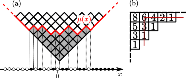
In the previous Section we have studied two particular cases—the strip-like configuration and a Lipschitz interface—for which the dynamical constraints emerging at infinite significantly simplify the evolution of the interface, which then can be described in terms of an equivalent 1 model. In this Section, we specialize the generic case discussed in Sec. III.2, by considering an interface shaped as in Fig. 4a, which is composed of two straight lines (parallel to the lattice directions) and a single, right-angled corner. This interface is Lipschitz-continuous in the sense of Eq. (16), and therefore the approach outlined in Sec. III.2 can be applied.
The case of a corner-shaped interface is particularly instructive, because of several connections to other fields of physics and mathematics:
-
1.
Its evolution can be thought of as the quantum counterpart of corner growth models studied in classical, non-equilibrium statistical mechanics [60, 53, 61, 62, 63]. These models describe the process of erosion of crystals; the case considered here extends the investigation of the melting phenomenon to quantum crystals [64, 65]. In fact, while a flat interface (of the type considered in Sec. III.2) can only fluctuate around its initial position, the corner configuration can be eroded indefinitely—if no other localization mechanism is present, as we will discuss below (see also Ref. [28]). However, in comparing the quantum to the classical case one should bear in mind that, for the quantum model under consideration, the addition/removal of a block from the corner (i.e. a spin flip) is always a coherent process, while in the classical problems the removed blocks “dephase” in the liquid state before being possibly reattached to the solid.
It is also interesting to notice the following feature. According to the stochastic dynamics, which is usually implemented for the classical Ising model (corresponding to Eq. (1) with ), the possible transitions between different spin configurations occur with a rate which is biased by (in a specific way that depends on the algorithm), where is the energy difference between the final and the initial configuration and the temperature of the bath. This implies, as expected on physical ground, that at zero temperature the possible transitions are those with . Assuming that the stochastic dynamics proceeds via randomly flipping single spins (as the coupling does in the quantum case), this implies that the allowed classical spin moves can be represented analogously to Eq. (7) as
-
(a)
, and for the fully reversible transitions with (or, more generally, for ). These are the moves contained in Eq. (7).
-
(b)
, its spatial rotations, and . These moves, occurring as indicated by the arrows, are not reversible and correspond to , with .
Moves of type (b) are not present in Eq. (7). However, it is easy to realize that, when considering an initial state with an interface in the form of a corner or, more generally of a Lipschitz function, these moves as well as the third type of moves in (a) are inconsequential, making the classical and the quantum dynamics actually explore the same set of configurations. In a heuristics sense, they share the same Krylov space of configurations in the -basis. As a consequence, the mapping discussed in Sec. III.2 and in Fig. 3 for the quantum interface can be applied also to the classical interface. This was done, e.g., in Refs. [63, 66, 67, 68]. The corresponding classical model is characterized by the classical equivalent of the fermionic statistics, i.e. by the constraint of exclusion in the occupation number of each lattice site which can be at most one, making it belonging to the general class of simple exclusion processes (SEPs) [53, 54, 62]. In the absence of the external field , the only allowed transitions starting from a corner (see Fig. 4a for the conventions) are and its reversed , corresponding to flipping a spin inside a corner from its two possible initial states. Such moves have the same rate, and therefore each classical particle in attempts jumps to the left or to the right empty neighbouring sites with the same rate, resulting in the so-called symmetric simple exclusion process (SSEP). Due to the intrinsic (unbiased) diffusive nature of ther dynamics, the growth of the interface turns out to be diffusive, while it is ballistic in the quantum case, as discussed further below. For , on the other hand, the transition and its reversed occur with different rates, depending on the sign and magnitude of . In particular, for it turns out that the only allowed moves are for and for . This corresponds to the classical particle jumping only towards the empty neighbouring site to the left or to the right depending on having or , i.e. to the so-called totally asymmetric simple exclusion process (TASEP). This model turns out to displays generically a ballistic growth (see, e.g. Ref. [63]), while the quantum dynamics is actually localized for . In addition, also the resulting limit shape is different: we discuss this aspect in more detail further below in this Section.
-
(a)
-
2.
Each configuration which is dynamically connected to the corner corresponds to a Young diagram, as detailed in Sec. IV.4. In particular, we will show an interesting connection between two seemingly unrelated measures on Young diagrams: the probability density of the quantum-fluctuating interface, which naturally emerges in the context of the Ising model, and the Plancherel measure, commonly studied in representation theory [69, 70, 71, 72, 73, 74, 75].
-
3.
Lastly, it is worth mentioning that the case of a Lipschitz interface, and in particular of a corner, the mapping to free fermions points to an explicit form of holography: a two-dimensional quantum problem in strong-coupling limit is mapped to a free, simpler problem in one less spatial dimension. This is reminiscent of the AdS/CFT duality [76, 77, 78]: the interface in the Ising model is the string in two spatial dimensions (plus time as an additional coordinate), while the non-interacting fermions on the chain are the dual field theory. When the string tension is large, the corresponding field theory is free. When the string tension decreases, the field theory becomes interacting and, in our case, no longer integrable.
However, in order to discuss the melting of a bubble and not of a simple corner, one has necessarily to introduce a more complicated theory of fermions, possibly with many species. It worth noticing that going back further in time, one finds other connections between the Ising model and string theory, for instance the conjecture that the Ising model should be dual to a weakly-coupled string theory [79, 80] (for a recent discussion see Ref. [81]), although that is supposed to hold only at the critical point.
Before passing on, we finally notice that the initial condition for the Ising model discussed in this Section actually corresponds to a single domain wall on the fermionic chain, which separates the filled part of the chain from the empty one. Let us emphasize that, for , this initial configuration is close to the boundary of the spectrum of the Hamiltonian within the Krylov sector it belongs to. Indeed, such configuration maximizes (or minimizes, depending on the sign of ) the expectation value of the Hamiltonian, being the state of maximal area of its Krylov sector. While in the limit this observation in marginal, as the system is integrable (thus any initial configuration leads to a non-ergodic behavior), it becomes relevant at finite , where the behavior of states at the middle of the spectrum can be also qualitatively different from the ones at the edges. This observation will be relevant in Secs. V.2–V.3 when discussing the finite- corrections.
IV.1 Average of the interface and its continuum limit
In the language of Sec. III.2, the corner-shaped initial state corresponds on the fermionic chain to
| (44) |
with a domain wall separating the empty half-chain for from the completely filled one at . In the language of electronics, this would be called a “maximum voltage bias” Fermi sea. By applying the approach previously illustrated (in particular Eq. (24)), one easily finds that the average density profile on the chain is given by
| (45) |
Summing over space (see Eq. (17)), one obtains the average interface profile
| (46) |
which, as anticipated, displays periodic oscillations with period at each position .
As discussed in Sec. III.3, in order to determine the continuum limit of Eqs. (45) and (46) it is then sufficient to replace by and therefore by in Eqs. (45)–(46), after reinstating the lattice spacing . Then the limit can be determined as explained in Sec. III.3. Alternatively, one can specialize the general prediction in Eq. (33) to the corner considered above, which corresponds to having, in the continuum,
| (47) |
i.e. a homogeneous spatial density of fermions equal to for and an empty lattice for . A straightforward integration leads to
| (48) |
which, for , agrees with the prediction of Ref. [82] for free fermions. Integrating over , one finds
| (49) |
with
| (50) |
Alternatively, this expression can be derived directly from Eq. (36), by using as the initial condition.
Equations (49) and (50) can be easily generalized to the case of a Lipschitz corner in which, however, the slopes of the interface in its two sides are not the same. On the lattice, this corresponds to having a certain average density of fermions on the left of the origin and a different one on its right. In fact, consider an initial profile which is linear for both and , but with two different slopes and , respectively, and that fulfils . Such a profile must take the form
| (51) |
The right-angled corner considered above corresponds to . With this , Eq. (36) implies that
| (52) |
where is given by Eq. (50). In fact, this expression simply follows from the linearity of the equation and from the result reported above for the right-angled corner.
Remarkably, the function in Eq. (50) first appeared in the context of random Young diagrams [69, 70, 71]; we will elaborate more on this point in Sec. IV.4. Here, instead, we comment on the connection between the dynamics studied above and the classical melting processes which were mentioned at point 1. of the introduction to this Section. In fact, in the cases of the SSEP or the TASEP, the stochastic dynamics starting from a completely filled half-line—corresponding to the dynamics at zero temperature of a corner in the Ising model—can be solved, obtaining the large-time behaviour of the density of particles (briefly reported in App. D). As anticipated at the beginning of this Section, the SSEP is, in a sense, the classical analogue of the quantum dynamics with , while the TASEP of the dynamics with . It turns out, however, that the scaling functions describing the erosion of the corner (which occurs diffusively for SSEP and ballistically for TASEP), via the same mapping described in Sec. III.2, have a different functional form compared to of Eq. (50) (see App. D). This fact highlights how the quantum and classical dynamics turn out to be quantitatively and qualitatively different in spite of their many similarities. In Sec. IV.4 we will discuss how this difference emerges also in terms of concentration of probability measures, showing that a simple entropic argument concerning the accessible configurations is not sufficient for explaining the limiting shapes of the interfaces, but that, as expected, also the classical or quantum nature of the underlying microscopic dynamics matters.
IV.2 Fluctuations of the interface
The approach described in the previous Section allows one to determine not only the average position of the quantum-fluctuating interface, but also its fluctuations. While presenting the complete calculation in App. C, we report here the final result for the connected two-point function of the density:
| (53) |
where we introduced the Bessel kernel
| (54) |
Note that, for , Eq. (53) straightforwardly reduces to
| (55) |
which is actually expected for fermionic particles. Summing over and in Eq. (53)—thus applying the prescription of Eq. (17)—leads to the connected 2-point function of the interface profile (Eq. (118)). In Fig. 5 we show the fluctuations of the interface profile: in panel (a) we present the value of as a function of position for different times, while in panel (b) we plot, for two values of along the chain, the average position of the interface with the corresponding fluctuations, over two periods of oscillation.

It is instructive to discuss the continuum limit also for the fluctuations of the shape . As they involve the Bessel kernel in Eq. (54), they are related to the universal fluctuations found e.g. in Laguerre and Jacobi ensembles of random matrices [83] (see also Ref. [84]), and of random representations of the symmetric group [73]. In particular, the presence of the Bessel functions implies a light-cone structure for the correlations, see Fig. 6a: if either or , the correlations are exponentially suppressed (as follows from the large-index asymptotic behavior of the Bessel function discussed in Eq. (101)). If, instead, both , then by virtue of the large-argument asymptotics of the Bessel functions presented in Eq. (102), the kernel reduces to the sine kernel
| (56) |
The sine kernel is found in numerous contexts in physics and mathematics, among which gaussian ensembles of random matrices [85], and free fermionic chains without a linear potential [86]. Notice that, in passing from the Bessel kernel to the sine kernel, the explicit dependence on has been lost in the expression for the correlations, while it remains implicit in the maximum value attained by or (i.e. the border of the light cone), see Fig. 6b. Finally, let us mention that a less trivial limit emerges in a region of order around the light cone, where by means of a uniform expansion (Eqs. (103)–(104)) the Bessel kernel reduces to the celebrated Airy kernel [87, 88].
Despite all the connections mentioned above, we need to emphasize that in this quantum setting the fluctuations are given by the square of the Bessel kernel, see Eq. (53): accordingly, they are quantitatively different from the cases mentioned above, which involve the kernels at their linear order.
IV.3 Entanglement dynamics
The “holographic” description of the interface in terms of an integrable 1 model (i.e. non-interacting fermions in a linear potential) allows one to extract much more information beyond averages and correlations, using the vast amount of analytical techniques developed in recent years [89, 90, 91, 92]. For instance, one can compute the so-called full counting statistics, i.e. the probability distribution of the fermions, with the techniques of Ref. [93]. In fact, it turns out that the predictions of Ref. [93] for the case carry over to our case just by replacing ; this “minimal” substitution is motivated by the fact that in the analytical expressions discussed in Sec. III.2 the time dependence occurred only via defined in Eq. (23), which encompasses both cases. Similarly, the growth of the entanglement across a bipartition of the lattice can be studied by using the results available for the problem [94]. In particular, one has to partition the lattice in two halves by means of a “vertical” line (e.g. through the corner, corresponding to the time axis in Fig. 6a), so that, on the chain, one has well defined subsystems. At this point, the entanglement of the and the problems are equal, as there is a one-to-one mapping linking all possible states in the two settings. The entanglement between the two subsystems can be computed as detailed in Ref. [94]: from the eigenvalues of the correlation matrix , the entanglement entropy is obtained as
| (57) |
The correlation matrix can be calculated explicitly, by using the properties of the Bessel functions which were used for calculating the average magnetization, with the result that
| (58) |
being the Bessel kernel of Eq. (54). If one computes the entanglement entropy between two subsystems and , separated by a vertical line in the problem, the indices of the correlation matrix are such that (or equivalently). For a bipartition located in , one has . Let us notice that the phase factor in the last equation does not affect the entanglement entropy; in fact, it can be removed via a unitary transformation. Accordingly, it is clear that the correlation matrix (and thus ) is a periodic function of time with period , as its time dependence is only through . Even if, to our knowledge, the eigenvalues of the correlation matrix of Eq. (58) cannot be obtained analytically, some analytical progress can be made in the continuum limit [95, 96]. Let us introduce the entanglement Hamiltonian such that
| (59) |
being the reduced density matrix of a subsystem , and a normalization constant. With this definition, one finds [97, 95, 98]
| (60) |
where is here the correlation matrix restricted to positions belonging to the considered subsystem . This means that and are diagonal in the same basis, and the corresponding eigenvalues satisfy the relation in Eq. (60).
As discussed also in Sec. IV.2, the Bessel kernel reduces to the sine kernel in the continuum limit inside the light cone. In this regime one can thus approximate the correlation matrix by setting to zero the entries with , and therefore one is left with an effective matrix of size , as depicted in Fig. 6b. Thanks to this approximation, one can obtain the eigenvalues of as [95, 86]
| (61) |
with . Denoting by the eigenvalues of , one has from Eq. (60)
| (62) |
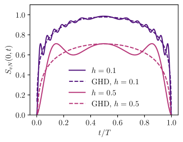
Note, however, that the asymptotic value Eq. (61) needs a very large to be accurate. For smaller values of , the eigenvalues vary as rather than , where are constants depending on the specific eigenvalue [95]. The evolution of the entanglement entropy can now be determined by using Eqs. (62) and (61) in Eq. (57). In Fig. 7 we show the numerical evaluation of the time evolution of the entanglement entropy, according to Eq. (57), for various values of . The presence of a non-vanishing external field implies that also the entanglement entropy is periodic in time.
We have shown how the mapping of the original problem onto a chain can be used in order to calculate the half-system entanglement entropy. However, the computation was possible only because of a convenient choice of the bipartition of the lattice (i.e. a vertical one in the rotated frame): more general bipartitions of the lattice would instead map non-locally on the chain. It seems that computing the entanglement of the system using the mapping into is viable as long as the cut along which the entanglement is computed is parallel to the projection performed in the mapping itself.
As a final point of this Section, it is worth noticing that the above results, valid in general on the lattice for arbitrary values of the couplings and , reduce, in the continuum limit , to the predictions of conformal field theory in curved space [99, 100] or quantum generalized hydrodynamics (GHD) [59]. The entanglement entropy is in fact given by
| (63) |
where and is the position of the bipartition. Equation (63) is clearly valid for ; otherwise, the entanglement entropy is zero because of the light-cone structure. In Fig. 7 we also compare the prediction given by Eq. (63) with the results of the exact diagonalization on the lattice, showing that a good agreement is attained for small values of , as expected. This relation was derived in Ref. [59] for ; the general case is obtained by means of the minimal substitution , coming from Eq. (23). In passing we mention that the GHD formalism allows one to predict the dynamics of one-dimensional integrable quantum systems directly in the continuum limit, even when the system is interacting; this is the reason why one needs the limit to match the GHD prediction.
IV.4 Connection with the asymptotics of the Plancherel measure
As pointed out at the beginning of Sec. IV, the states in the Krylov sector connected with the infinite corner are in one-to-one correspondence with Young diagrams (also known as Ferrers diagrams). By definition, a Young diagram is a collection of boxes, arranged in a sequence of left-justified rows of non-increasing length [101]. Young diagrams are a graphical tool commonly used to represent integer partitions, to compute dimensions of group representations, and for many other mathematical purposes [101].
In order to discuss the connection with the present work, let us recall here some basic facts concerning Young diagrams. A partition of an integer indicates a possible decomposition of as a sum of positive integers, i.e.
| (64) |
Representing each integer as a string of adjacent boxes , one can easily see that a partition corresponds to a Young diagram, obtained by stacking all the strings, starting from the first. A theorem [101] states that the irreducible representations of the symmetric group of degree are labelled by the possible partitions of size . Moreover, the dimension of the representation corresponding to a certain can be obtained via the hook length formula
| (65) |
where is the so-called hook of the square [101], an integer number determined as explained in Fig. 4b.
For our purposes, the most interesting interpretation of resides in the fact that it gives the number of ways in which the diagram can be constructed, starting from the empty diagram, by adding one square at a time in such a way that at each step one still has a partition [102]. In the mathematical literature, it is common to define the Plancherel measure on the set of partitions as [69, 70, 71, 72, 73]
| (66) |
which is proved to be a normalized measure, i.e. a probability [103].
An important result of combinatorics is that the Plancherel measure concentrates at large , i.e. it becomes a delta function on a particular set of diagrams [69, 70, 71, 72, 73]. The diagrams belonging to this set have approximately the same shape; more precisely, after a counterclockwise rotation of the diagrams (such that they are finally arranged as in Fig. 4a) their shape is actually described by the function with given in Eq. (50). It is thus quite surprising to find another, completely different growth process that leads to the same limiting shape as the one induced by the quantum dynamics of the Ising model.
While we could not devise a mathematically rigorous proof, we heuristically understand the above correspondence as follows. Recalling that gives the number of paths that reach the diagram from the empty one, always remaining within the set of Young diagrams, we notice that the Plancherel measure weights each diagram with the square of the number of paths. On the other hand, one can consider the Green’s function
| (67) |
where we denoted with the Hamiltonian in Eq. (7), making explicit the dependence on , and and are two Young diagrams. Performing the locator expansion of the resolvent [104, 105, 106, 28]
| (68) |
where denotes the set of paths in configuration space from to , is the length of the path and we introduced the notation , i.e. denotes the energy of in the absence of hopping (). In the spirit of the forward approximation [105, 106, 28], one can approximate the sum in Eq. (68) by reducing to , i.e. the set of shortest paths from to . This corresponds to work at the lowest order in the hopping . Under this assumption, the argument of the sum does no longer depend on the specific path, but only on its length , because all the diagrams with a fixed number of blocks, viz. at the same distance form the empty diagram, have the same energy , see Eq. (7). This means that the sum gives the number of shortest paths from to (with , otherwise it gives zero). Specializing Eq. (68) to the case of the path from the empty diagram (with ) to (), one finds
| (69) |
where, in the second line, we used the fact that . Taking the residue of this propagator at , one finds the expression of the corresponding eigenfunction
| (70) |
Accordingly, the probability of being in the state turns out to be proportional to —i.e. to the square of the number of paths leading to it, according to the interpretation of —and therefore to the Plancharel measure in Eq. (66). This motivates the connection between the quantum dynamics and the Plancherel measure concentration.
Before passing to the next Section, it is interesting to note that the forward approximation also gives the correct result for the decay of the eigenfunctions upon increasing . To see this, one must plug in Eq. (70) the value of , which clearly depends on the specific form of the diagram associated with the state . Referring for details to Ref. [71], we just say here that it is possible to provide an upper (resp. lower) bound to the maximal (resp. typical) value of : in both cases, the leading term scales as . Using Eq. (70), one gets that the eigenfunctions approach zero faster than exponentially upon increasing , because of the overall factor . This estimate is in agreement with the exact result of Eq. (19), since the Bessel functions decay as the inverse factorial of the (large) index, see Eq. (101).
V Mechanisms of integrability breaking
In the previous Sections we showed that the Hilbert space of the Ising model in the infinite-coupling limit shatters in many disconnected Krylov sectors. Among these sectors, those corresponding to the wide class of interfaces discussed in Sec. III.2 can be mapped onto a model which turns out to be integrable. In this Section we discuss the dynamics of the interface beyond integrability and the robustness of the qualitative features of the exact solution, presenting in detail what was briefly anticipated in Ref. [16] by us.
In Sec. V.1 we argue that the interfaces which do not satisfy the Lipschitz condition of Eq. (16) may have a very different dynamical behaviour compared to the one described so far, because they can break into disconnected pieces. This is done by considering the case of an interface which is locally Lipschitz, but which it is not the graph of a function at a larger scale. In Sec. V.2 we consider, instead, another possible source of integrability breaking: the presence of a finite, albeit still large, coupling . Specifically, we will discuss the corrections to the infinite-coupling Hamiltonian (3) and address the ergodicity of the resulting model. In Sec. V.3 we discuss, using both analytical and numerical techniques, why the corrections to the infinite-coupling Hamiltonian lead to a localization phenomenon, named Stark MBL, induced by the presence of the longitudinal field . Finally, in Sec. V.4 we compare our results for the time evolution of a domain on the lattice with the equivalent problem in the continuum, studied in the context of the false vacuum decay scenario, highlighting qualitative differences.
V.1 Finite bubbles
Throughout Secs. III.2 to IV.4 we assumed the presence of a single interface, separating the lattice in two infinitely extended domains. It is then natural to investigate the extent to which the predictions derived therein carry over to finite domains. The easiest and natural case to be considered is that of a single, large bubble of “down” spins, surrounded by “up” spins (or vice-versa). Let us also introduce the notion of convexity on the lattice: we will say that a domain is convex if any line parallel to the lattice axes joining two points in the domain lies entirely within the domain itself. As already noted in Refs. [18, 16], all convex bubbles are dynamically connected with the minimal rectangle (with sides parallel to the lattice axes) that contains them, i.e. they belong to the Krylov sector generated by this rectangle. Moreover, because of the perimeter constraint, the domain-wall dynamics is always confined within such a rectangle. Accordingly, we can directly assume that the shape of the bubble at the initial time is a rectangle, as all the other cases will follow from this one.
The early-stage dynamics of such a rectangular bubble can be predicted on the basis of the previous analysis. In fact, the sides of the bubble are immobile, since no spin can be flipped without modifying the perimeter, while the corners start to be eroded, as discussed in Sec. IV. However, the evolution will deviate from that of an infinite and isolated corner as soon as two adjacent corners will start “feeling” the presence of the other. The timescale at which this happens can be be bounded from below by computing, in the fermionic language, the probability of finding two fermions, each coming from a different isolated corner, halfway along the flat portion of the interface which connects these two corners.
Let us denote by the length of the shortest side of the rectangular, finite bubble. There are now two possible cases. If the longitudinal field or, more generally, is small enough for the Bloch oscillations to have an amplitude (Eq. (26)) larger than the distance , then the excitations propagate ballistically on the chain with speed (Eq. (49)), and they meet at after a time
| (71) |
If, instead, is nonzero and large enough to confine the dynamics in a region smaller than , one can estimate the probability of having a fermion at a distance from the corner (equivalently, a hole at distance ) with . On the maxima of the oscillations of the corresponding interface 555A very similar result is obtained if taking the average over a period, rather than the maximum of the oscillations., attained at times such that (Eqs. (23) and (49)), one finds , cf. Eq. (45), and consequently
| (72) |
Recalling that the Bessel functions of large order decay exponentially fast to zero, one can approximate (see also Eq. (101))
| (73) |
With this result, the typical time after which two fermions, coming from different corners, interact can be estimated as or, more explicitly 666This result can be obtained using Fermi Golden Rule. In particular, the interaction rate for two fermions coming from different corners is proportional to the probability of having both fermions at half chain. Being fermions of different species, they interact only at the scattering point and therefore such probability is the product of the single fermion probability of being at distance from the corner. Consequently, taking the inverse of the rate, one obtains .,
| (74) |
One can see that, in the case , a time which is more than exponentially large in the bubble size must pass, before integrability breaking starts to be manifest.
It is natural to wonder what happens to the bubble after this timescale. Based on elementary reasoning, one can argue that two kinds of processes may take place: (a) the excitations coming from one corner may start to affect the dynamics of adjacent corners, transferring energy between corners and deteriorating the perfect coherence of the single-corner oscillations; (b) the interface may break because of the detachment of isolated bubbles of flipped spins caused by the interface-splitting transitions of Eq. (7). We note, however, that these detached parts can move away from the parent interface only via processes. A detailed study of this challenging problem is left for future investigations.
We conclude by emphasising that the case of two adjacent corners we have considered here actually applies to any very large bubble, provided that its boundaries are “smooth” enough—i.e., that the Lipschitz condition is locally satisfied while the points responsible for its global violation are very dilute. If, instead, the initial interface is rather corrugated, i.e. it is not the graph of a function even locally, then we expect a really complicate time evolution, during which all accessible configurations may be explored, and the single-interface description is no longer possible.
V.2 Finite coupling
We now relax the assumption that be strictly infinite, considering the effects of the corrections , but still under the assumption that .
A large but finite still imposes an effective dynamical constraint, valid up to a timescale which become exponentially long upon increasing : this follows from the rigorous prethermalization bounds of Ref. [109]. Specifically, the perturbatively “dressed” version of the domain-wall length operator (defined in Eq. (2)), arising from the Schrieffer-Wolff transformation, is accurately conserved for a long time that scales (at least) exponentially:
| (75) |
(here and are numerical constants independent of , , and ). This is because the Schrieffer-Wolff effective Hamiltonian , computed up to a suitable optimal perturbative order, commutes with in Eq. (2) up to an exponentially small error [109]. In addition, the evolution of all local observables is well approximated by for [109].
As anticipated above, the zeroth order of the Schrieffer-Wolff effective Hamiltonian was already determined in Sec. II.2 and is given by Eq. (3). Computing higher-order corrections to becomes rapidly very complex, as the number of terms increases more than exponentially. In App. E.1 we sketch the computation of the first-order corrections in , while in App. E.2 we specialize it to the dynamical sector of a smooth interface, of the type defined in Sec. III.2. In this sector, the perturbative corrections takes a simpler form. The construction above can be translated in the fermionic representation. The Schrieffer-Wolff effective Hamiltonian
| (76) |
has the zeroth-order contribution given by Eq. (18), while the first-order corrections turn out to be
| (77) |
One may recognize that they entail next-nearest-neighbour hoppings and density-density interactions. One can notice also that the density-density interactions, which are diagonal in the occupation number basis, do not depend on . Consequently, the addition of the first-order corrections breaks the symmetry: changing the sign of modifies the expectation value of the energy. The terms in are rather generic, and therefore one naturally expects them to break the integrability of the model, and make it thermalize rather quickly. However, as we anticipated in Ref. [16], if is sufficiently large the perturbation is not able to restore ergodicity. In the next Section we describe this phenomenon in detail.
Let us briefly mention that, upon including the corrections, an isolated flipped spin can spread in the lattice with a hopping amplitude . This means that it is no longer possible to provide an effective description even for initial configurations of the strip-like form, discussed in Sec. III.1 for .
Before continuing, it is important to emphasize a fundamental issue with the Schrieffer-Wolff transformation. For large but finite , the dynamics of the initial product states considered so far in the form of the classical configurations will exhibit vacuum fluctuations even away from the existing domain walls. This is due to the perturbative dressing of the bare ferromagnetic state by virtual spin excitations. In practice, this arises from the application of the Schrieffer-Wolff unitary transformation , c.f. Eq. (138), to the fully polarized initial product state. Accordingly, for such initial states one should think of the ferromagnetic vacua (i.e. those on the two sides of an infinite interface or the inner and outer regions of a bubble) as superpositions of dilute spin flip excitations, of spatial density . Such excitations can be described as magnons, hopping on the lattice with amplitude . In principle this dilute magnon gas contributes to the dynamics of the interface, but in the following we will ignore this fact, leaving its discussion to future investigations. This choice actually corresponds to taking as the initial state an interface in the the Schrieffer-Wolff transformed basis, rather than in the classical one discussed so far.
V.3 Arguments in favour of Stark many-body localization
The goal of this Section is to study the evolution induced by the Hamiltonian (76). The first term in Eq. (76) is the Hamiltonian considered already in Secs. III.2 and IV: it represents a chain of Stark-Wannier-localized, non-interacting fermions. The second term, i.e. of Eq. (V.2), is a small perturbation containing both next-nearest-neighbour hoppings and two-body interactions. Accordingly, there is a competition between the localized nature of the dynamics induced by and the interactions in , which are generally expected to drive the system towards a thermal phase. Previous works [19, 20, 110] have shown that, for interacting Hamiltonians very similar to Eq. (76), an extended non-thermal phase is present for sufficiently strong field , partly in analogy to what happens in the disorder-induced many-body localization (MBL). Indeed, the phenomenon has been dubbed Stark MBL.
In order to quantify the competition between interactions and the linear potential responsible for the localization, we developed an analytical argument à la Basko-Aleiner-Altshuler (BAA) [21] which goes as follows. Start from the integrable limit : the eigenfunctions are expressed in terms of the single-particle orbitals of Eq. (19) and are all spatially localized. Their localization length can be quantified by the participation ratio: using Eq. (19) and Neumann’s addition theorem (see App. B),
| (78) |
where is given after Eq. (19). An approximate form of this relation is derived in App. F, where we perform the asymptotic expansion of the above integral for large values of through the method of the Mellin transform, determining
| (79) |
where and is the Euler-Mascheroni constant. Such approximation is clearly accurate for , i.e. for small .
We now assume that one can partition the system into boxes (“quantum dots”) of size , as sketched in Fig. 8. Within each of them, the number of states is clearly (there are sites that can be either empty or occupied), whereas the maximum energy difference between two many-particle states is . To understand this latter estimate, assume : then, the minimum energy is attained when no particle is present (), while the maximum when all sites are occupied (and thus ). With the same reasoning, with one gets , thus confirming the estimate.
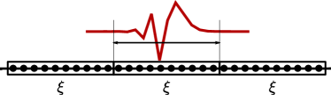
Following BAA (and thus also building on Ref. [111]), we say that interactions should not be able to restore ergodicity (at least perturbatively) if their strength is smaller than the average local level spacing:
| (80) |
i.e. when . This is equivalent to requiring
| (81) |
which is always satisfied for , i.e. for sufficiently large . It is interesting to note that the regime of validity of the heuristic criterion (81) depends only weakly on . In Fig. 9 we show, upon varying and , the regions of validity of the inequality (81), where is given by Eq. (78). One can observe how, for fixed , the criterion is satisfied for sufficiently large ; moreover, for , the condition in Eq. (81) holds for .

As a check for the above estimate, we performed numerical simulations, focusing in particular on the “generalized imbalance”, a witness of ergodicity breaking. Given a generic initial state , the time-evolved generalized imbalance for a system of length is
| (82) |
where we defined . If the initial state is a Néel state, then the generalized imbalance reduces to the standard imbalance between the occupation number of odd and even sites, used both in numerical simulations and cold-atom experiments. Taking the infinite-size limit and averaging over time, one obtains
| (83) |
which is zero in generic thermalizing systems. Accordingly, is a sufficient condition for the system to be non-ergodic (even if it is not necessary). The infinite-time limit in the definition of can be obtained also by using the diagonal ensemble: assuming to be given as in Eq. (21), one finds
| (84) |
with the average defined in Eq. (25), and the eigenbasis of the Hamiltonian Eq. (18).
The ergodicity test based on the valuer of should in principle be done for every initial configuration. However, there are states that will trivially give a non-ergodic result . For example, states near the ground state will remain non-ergodic also in the presence of the corrections, just because they lie at the edges of the spectrum: we checked numerically that this is the case, for instance, for the domain-wall state of Eq. (44) (data not shown). A non-trivial test, instead, is provided by generic states which lie in the middle of the spectrum: for our purposes, the Néel state , for which , will suffice.
In Fig. 10 we compare the numerical values of at finite , with the analytical prediction at : using the definition in Eq. (82) and Eq. (92) one finds
| (85) |
In the long-time limit, the temporal average of is given by
| (86) |
where the last step is a known property of the Bessel functions [112], see Eq. (110).
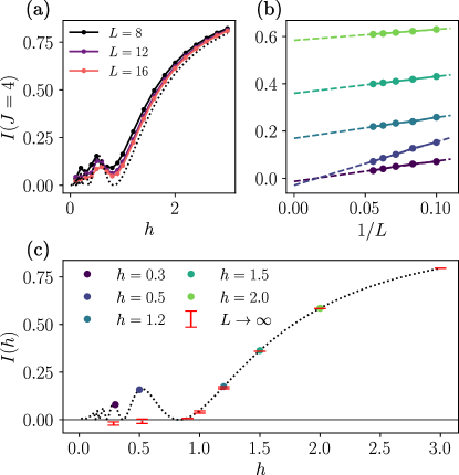
The curve is represented, for , by the dashed lines in Figs. 10a and 10c. For finite values of , instead, one is able to compute the generalized imbalance only numerically and for finite . Accordingly, the estimate for has to be obtained via extrapolation, which we perform in Fig. 10b. The numerical values of the generalized imbalance show a linear dependence on , allowing for a reliable extrapolation to (see the caption of Fig. 10 for more details). The final results are reported in Fig. 10c: while for the generalized imbalance is compatible with , for the results at finite are perfectly compatible with the analytic prediction at . These data provide numerical support to the argument à la BAA that we discussed above. In addition, we performed also numerical simulations for the time evolution of the generalized imbalance (which we do not report here), and we noticed that the relaxation time to the diagonal ensemble value depends on (the larger , the longer the time needed), whereas the asymptotic value does not, again in agreement with the argument á la BAA.
V.4 Implication for the dynamics of finite bubbles and the decay of false vacuum
As mentioned in the Introduction, the problem addressed in the previous Sections is reminiscent of the false vacuum decay process, that received much attention in the field theory context, in particular starting from the works by Coleman [5, 6, 7]. In our work, we started directly from the situation in which a true vacuum bubble is already present in the false vacuum (or false vacuum in the true vacuum, which is equivalent in our setting). Therefore, we will not discuss here the timescale needed to create a bubble out of a uniform configuration (for the quantum Ising model this issue has been addressed in Refs. [113, 114]). Here we will limit ourselves to compare the evolution of such domains on the lattice and in the continuum, the latter problem being solved in Ref. [5].
Let us start by reminding the reader that a false vacuum, i.e. the state in which the spins are uniformly aligned in opposite direction to the longitudinal field, is a highly-excited state with finite energy density, which is expected to decay to configurations with equal total energy but larger entropy. Coleman identified and described this kind of decay process occurring in a field theory as the generation of a resonant true-vacuum bubble(s), the critical linear size of which is determined by the balance between the energetic cost for creating its interface ( in our setup), and the bulk energy gain in having a bubble of true vacuum (in our setup, this comes from the the spin alignment, with gain ). The value of the critical linear size of the bubble is easily found: .
In continuous space-time, the timescale associated with the formation of the bubble above can be calculated in the framework of relativistic quantum field theory using instantons. The total potential energy change , which vanishes at the moment of the formation of the bubble, starts decreasing to large negative values when the bubble increases its dimension and accelerates quickly to swallow the remaining false vacuum, transforming the gained potential energy in kinetic energy so that the total energy does not change, i.e., . However, there are considerable differences between our lattice setting and what happens in a field theory on the continuum. First of all, in the limit it is easily seen that and therefore the bubble is not formed at all. But, for finite , if one waits a time exponentially large in (using the result from Coleman’s continuum calculations), the bubble will eventually form. The walls are now expected to accelerate, expanding the bubble indefinitely, accumulating excess potential energy in a way which conserves the total energy. This expansion and acceleration, however, cannot occur on the lattice: as it can be seen from the dual fermionic description, the kinetic energy of the domain wall is actually bounded on the lattice by the value of , and this prevents an expansion to sizes larger than . This is the reason why the bubble starts oscillating. We have proven in this paper that these oscillations survive the perturbative introduction of a finite , because the mechanism of Stark MBL confines the holographic fermions. With finite , , and , instead, Coleman’s results for the expansion and the acceleration must proceed on timescales which are exponentially large (non-perturbative) in . Our best attempt at calculating this rate is in Sec. V. In the simpler case of spin chains, in fact, it was found that Bloch oscillations also inhibit the expansion of the true vacuum bubble [29, 30, 115]. Accordingly, the post-vacuum-decay scenario ought to be profoundly different from that described by Coleman.
VI Conclusions
In this work we have shown, expanding on the results of Ref. [16], how to describe the dynamics of interfaces in the two-dimensional quantum Ising model with strong ferromagnetic coupling . As a first step, we discussed the infinite-coupling limit , focusing both on the equilibrium properties of linear spin domains embedded in the lattice, and on the dynamics of infinite interfaces described by Lipschitz-continuous functions. In the first case, we have shown that the model reduces to a PXP Hamiltonian, for which one can calculate exactly the equilibrium magnetization, assuming that the initial state has negligible overlap with quantum many-body scars. The interest in the second case, instead, has a twofold motivation: first, the corresponding configurations effectively describe smooth interfaces and, second, given the impossibility of breaking the domain wall (ensured by the Lipschitz condition which is conserved by the dynamics), an effective description can be provided in terms of fermionic particles subject to a linear potential, which is amenable to an exact solution. We also discussed how to take the continuum limit of the dynamics, in order to predict the behaviour of the quantum-fluctuating interface at scales much larger than the lattice spacing. A semiclassical interpretation of the resulting formula naturally emerged.
Then, we moved to the case of an interface shaped like an infinite corner. In particular, we discussed the properties of the average limiting shape, both on the lattice and in the continuum, and its relationship with classical corner growth models. We predicted the dynamics of the entanglement entropy between the two halves of the corner, and unveiled a deep connection between the quantum problem and the asymptotics of the Plancherel measure on random Young diagrams.
We finally relaxed the assumption of infinite strength of the Ising coupling , making use of a Schrieffer-Wolff transformation to calculate the corrections. The first-order corrections break the integrability of the model with but, remarkably, ergodicity is not restored. In fact, the presence of the longitudinal magnetic field in , which translates into a linear potential in , causes the emergence of Stark MBL, that we characterized both numerically, computing the generalized imbalance, and analytically, providing an argument for its validity. Even if a recent work provided analytical evidence against Stark MBL [116], their results apply only to the infinite-time limit, where our perturbation theory in is no longer reliable. We expect therefore that, on the timescales considered in this work, the phenomenology of localization is quite robust.
In order to understand the temporal range of validity of our predictions, we investigated the relevant timescales controlling the dynamics of the system in generic conditions. In particular, we identified in the prethermal timescale, after which the description in terms of Schrieffer-Wolff expansion is no longer valid: it turned out that becomes (at least) exponentially long upon increasing . Moreover, the possibility of utilizing a chain to describe interfaces in is justified as long as the effects of possibly having a finite bubble size are negligible. Accordingly, we estimated the timescale below which this is a reliable assumption, and turned out to increase more than exponentially upon increasing the linear size of the domain. Both these timescales ensure that the results presented here, which were derived in the infinite-coupling or infinite-size limits, actually carry over to the case with finite but “large” coupling and sizes, up to very long times.
An intriguing question is about the dynamical effects arising at times longer than and . While we leave this problem to future work, we can argue that the description given here is no longer valid, as the interface-splitting moves start playing a major role, and even the conservation of the interface length is no longer strictly guaranteed. As a consequence, the possibility of employing a chain to describe the dynamics of a generic domain will likely be lost. However, for some initial configurations or at least in some regimes, we expect that it will still be possible to give a description in terms of a effective problem, as we hope to address in a future work.
Let us conclude by noting that, in the general case, the full nature of the problem will emerge in the long-time limit, or for generic couplings. In these regimes no description will be reliable and new techniques will be needed. Ultimately, it is natural to expect that a complete solution of the quantum Ising model is at least as hard as the solution of the classical Ising model.
Acknowledgements.
F.B. and C.V. would like to thank P. Calabrese, L. Capizzi, G. Di Giulio, G. Giachetti, A. Santini and S. Scopa for useful discussions.Appendix A Magnetization in the linear strip
We provide here a more detailed analysis of the dynamics of a linear strip of spins, treated in Sec. III.1.
Let us start from the computation of the number of dynamically accessible configurations for a strip of spins of length , in which spins are flipped compared to the initial configuration: due to the perimeter constraint, satisfies Eq. (9). This recursion relation is actually obtained by summing the number of configurations in which the -th spin along the chain is not flipped (we recall that the -th spin cannot flip) and the number of configurations in which it is flipped. As there is only one configuration with no spin flip, the initial condition for Eq. (9) is and its solution is thus given by Eq. (10): this is a direct consequence of Pascal’s property of the binomial coefficient [117]. In order to determine the total number of accessible configurations starting from the strip, one needs also to know the maximum number of spins that can be flipped without violating the perimeter constraint. As anticipated above, the first and last spin cannot flip, and therefore one is left with potentially “active” spins. If is even, one can flip at most alternating spins, whereas if is odd, one can flip alternating spins. Accordingly, is given by Eq. (11) in the main text.
Under the assumption of an ergodic dynamics (see the main text), the magnetization profile can be determined by using the following argument. Consider the -th spin of a chain of length . The number of configurations having the -th spin “up” are given by the total number of allowed configurations for the two sub-chains (consisting of and spins, respectively) split by the -th spin, that is . In the remaining allowed configurations of the strip the -th spin is down, and therefore the magnetization at site is simply given by
| (87) |
as reported in Eq. (13), with the reflection symmetry and the boundary condition . Using the explicit expression of the Fibonacci numbers in Eq. (14), one gets, for
| (88) |
being the golden ratio. In the limit , one finds the magnetization at center of the strip to be given by Eq. (15), after using the expression of the golden ratio provided before Eq. (14). The dependence on of Eq. (88) also implies that the approach to this asymptotic value is exponential with the typical length indicated after Eq. (15).
Appendix B Useful properties of the Bessel functions
In this Appendix we collect a number of properties of Bessel functions which are useful and widely used to derive the results presented in the main text, and we provide also a sketch of their proofs. Many of these properties can actually be found in Refs. [112, 118, 119].
One of the equivalent definitions of the Bessel function of the first kind is in terms of the integral:
| (89) |
From this definition it follows immediately that
| (90) |
, and, for ,
| (91) |
Using again the definition, one can compute the following relation, useful in the calculation of the average of the number operator in Eq. (24), Sec. III.2
| (92) | ||||
| (93) | ||||
| (94) | ||||
| (95) |
where we used . Setting we obtain the completeness relation
| (96) |
that also leads immediately to
| (97) |
If the sums of the previous equation is restricted to positive integer values, using telescopic sums one obtains
| (98) |
that reduces to
| (99) |
when the limit is taken. This relations allows us to compute explicitly the fluctuations of the number operator in Eq. (115), App. C. Using the same procedure as in Eq. (92) we can compute also
| (100) |
Another very useful tool is the asymptotic expansion of the Bessel functions for large order and argument (see Ref. [112]), which are useful for discussing the continuum limit of the dynamics in Sec. III.3. For fixed and one finds
| (101) |
i.e. the Bessel functions vanish faster than exponentially upon increasing . In the limit with fixed , instead, we have, at the leading order
| (102) |
If both the order and the argument of the Bessel function diverge, the asymptotic expansion is different if the argument is larger than the order or vice versa: at the leading order for , one has
| (103) | |||
| (104) |
from which we notice the strong similarity between Eqs. (101)–(103) and Eqs. (102)–(104). This means that the asymptotic expansions of the Bessel function remain unaltered even when both the argument and the order scale linearly, but with different powers. Indeed, to see the transition between the regimes described by Eqs. (103) and (104) one has to consider for and fixed , which is not important for our discussions. For the purpose of taking the continuum limit as explained in Sec. III.3 and Sec. IV.1 we note that Eqs. (103) and (104) imply that, in the limit with fixed , one has
| (105) |
where is the unit step function which equals 1 for and vanishes otherwise. This equality is valid after integration with a smooth function, i.e. in the sense of distributions. In fact, the rapidly oscillating term deriving from Eq. (104) has been replaced with its average value , while the rapidly decaying exponential in Eq. (103) has been set to zero, as indicated by which appears in the expression above.
Another useful formula is
| (106) |
which is used in Eq. (78). In order to prove it, one can use a modified version of Neumann’s addition theorem, i.e. the Graf’s and Gegenbauer’s addition theorem [112]
| (107) |
By setting , taking the square of both sides, and taking the angular average for , one gets
| (108) |
thus proving the identity.
Appendix C Two-point functions
In order to obtain the fluctuations of the limiting shape of the Young’s diagrams, one needs the 2-point function of the number operator , see also Eq. (17). For simplicity, we report here the computation done at equal times, but the same procedure can be extended also for different times. Let us start by computing
| (111) |
Also in this case, one can expand the initial state and use the time evolution of the fermionic operators. The expectation value one gets, using Wick contractions, is
| (112) |
being, by definition,
| (113) |
After some straightforward steps one arrives at
| (114) |
being , as in the main text. Therefore, the connected 2-point function is
| (115) |
Using Eq. (98), one arrives at (see also Ref. [120])
| (116) |
The fluctuations of the number operator of the fermions along the chain is readily obtained from Eq. (114) by setting :
| (117) |
At this point, summing over space as it was done before, one arrives at the correlation function for the shape operator
| (118) | ||||
| (119) |
With the same procedure one can compute the expectation value of the current operator, defined as:
| (120) |
Using this definition, one obtains
| (121) |
At it reduces to
| (122) |
Also the current-current correlator can be computed with the same tools: we report here the result for , which is given by
| (123) |
Appendix D Comparison with classical simple exclusion processes
In this Appendix we compare the predictions presented in Sec. IV.1 for the dynamics of the corner-shaped interface in the quantum Ising model, with those obtained for the classical simple exclusion processes (SEP) which, as discussed in the main text, represents the classical counterpart of the quantum Hamiltonian (18). In particular, we focus on the totally asymmetric simple exclusion process (TASEP) and the symmetric exclusion process (SSEP), discussing them in the appropriate continuum limits, which makes the comparison with Eqs. (48) and (49) immediate. For a discussion of these processes on the lattice, instead, we refer to the vast literature on the topic, e.g. Refs. [121, 122, 55, 123, 124, 68].
First, we note that, while the time evolution of the TASEP is ballistic [125], the one of SSEP is characterized by a diffusive scaling [126, 124]. Denoting respectively by and the density of particles and the interface height (as in Eq. (17)), it turns out [125] that the dynamics of the rescaled density
| (124) |
of the TASEP (the subscript stands for TASEP) obeys the Burgers equation
| (125) |
We have denoted with the average number of particles on the lattice, while denotes the average number in the continuum, which is obtained by taking the limit in Eq. (124), where is the inverse of the lattice spacing. With the step initial condition —corresponding to the corner—one obtains the solution , with the scaling function
| (126) |
The corresponding interface height , determined according to Eq. (17) on the continuum, turns out to be given by , with the scaling function
| (127) |
In the case of the SSEP, instead, the dynamics is diffusive and a different scaling of space and time has to be taken in order to obtain a non-trivial continuum limit. Specifically, the rescaled density , (the subscript stands for SSEP) satisfies the heat equation [126]
| (128) |
The same initial condition as before, i.e. , leads to the solution with the scaling function
| (129) |
where we introduced the error function . According to the continuum version of Eq. (17), the interface profile is given by , with the scaling function
| (130) |
In Fig. 11 we compare the scaling forms obtained above for TASEP and SSEP with the one of the quantum model. In doing this comparison one should remember that the very scaling variables differ in the various cases with the sole exception of TASEP and the quantum Ising model with : in spite of the fact that they both show a ballistic scaling, the corresponding scaling functions are still different.
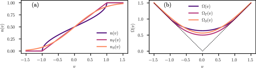
Appendix E Second order Schrieffer-Wolff and integrability breaking
In this Section, we perform a Schrieffer-Wolff transformation [35] to get a renormalized Hamiltonian, describing the effective degrees of freedom in each sector when . We remind that the Schrieffer-Wolff transformation consists in a renormalization procedure that progressively eliminates, order by order in perturbation theory, all the block-off-diagonal Hamiltonian matrix elements, i.e. the ones coupling different sectors and with . Mathematically, it is a unitary rotation , with , that gives
| (131) |
where and are of order in the perturbative coupling. Moreover, performing the expansion up to a finite yields a rotated Hamiltonian in which the block-off-diagonal terms are of order or higher.
We will follow a recent derivation of the transformation, given in Refs. [109, 30], that gives directly the correct result at any desired order.
E.1 First-order corrections: PXP Hamiltonian
Let us start by separating the original Ising Hamiltonian in Eq. (1) as follows:
| (132) |
Setting, for the time being, , the Schrieffer-Wolff transformation amounts to the following iterative algorithm (starting from ):
-
1.
Split , where contains only the block-diagonal terms and only the block-off-diagonal ones.
-
2.
Determine from the equation
(133) -
3.
Set
(134) where the summations run over the set of the ordered partitions of an integer , and excludes the partition with .
Let us apply the algorithm described above to our case, up to order . First of all, we identify in the block-diagonal terms:
| (135) | ||||
and the block-off-diagonal terms:
| (136) |
In the previous equations, the projectors are those given in Eq. (4), while stands for the left/right/above/below neighbour of the site , as in the main text. One easily gets convinced that the terms in couple states within each , since they conserve the number of domain walls; contrarily, each term in changes their number.
Then, we need to solve Eq. (133), specified for :
| (137) |
A bit of reasoning leads to the conclusion that one can compensate each term in , of the form , with a term in of the form . Fixing the correct signs, one finds
| (138) |
Finally, applying Eq. (134) for yields
| (139) |
The expression above generates a plethora of terms; however, we are interested only in the block-diagonal part of , namely : indeed, the block-off-diagonal part can be removed by going to the next order in the perturbative construction. For now, we will compute only the terms in Eq. (139) that are diagonal in (thus leaving out terms involving and that are still block-diagonal). It is easy to identify them, since they come from commuting in and with in , while leaving the projectors untouched (and therefore the 4 projectors around have to be the same both in , and ). With a bit of patience, one may work out all the details, finding
| (140) |
E.2 First-order corrections: corner Hamiltonian
Now we specify the expression derived in the previous Section to the sector within which is dynamically connected to the corner considered in the main text, i.e. we restrict our attention to the Young diagrams subspace . In the previous Section we have already determined the diagonal part of the second-order correction , see Eq. (140). We just need to determine the off-diagonal (but block-diagonal) part. With a bit of reasoning, one may get convinced that the only allowed moves at the second-order perturbation theory, which bring a state out of and then back in, are those represented in Fig. 12. Correspondingly, the Schrieffer-Wolff Hamiltonian reads
| (141) |
The factor in front of the sum is fixed by a careful use of Eq. (139). Now that we have the Hamiltonian in , we can express it in the language of fermions. Before, however, it is convenient to expand all the projectors in terms of : one finds
| (142) |
The term with only two Pauli matrices gives a constant contribution on the Young diagram states, since it counts the number of horizontal and vertical frustrated bonds (it is a constant energy shift in the whole sector ). The term with four spins, instead, can be represented, up to a constant term in the subspace , by an operator which counts the number of corners in each diagram. Accordingly, in the fermion language, one finds the Hamiltonian
| (143) | ||||
| (144) |
where the first term is a correction to the kinetic energy and the second a four-fermions interaction.
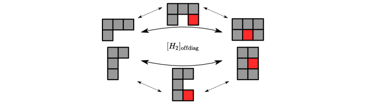
Appendix F Participation ratio and localization length
In this Section we compute the (inverse) participation ratio, from which one can easily derive the localization length of the eigenfunctions. By definition
| (145) |
where we used both Neumann’s addition theorem to write the sum as an integral and the explicit form of the eigenfunctions. With a change of variables, the integral can be cast in the form
| (146) |
where is the generalized hypergeometric function. For large , one can take the asymptotic expansion of the latter and the (non-oscillating part of the) turns out to be given by
| (147) |
being the Euler constant. Since the localization length of the eigenfunctions is roughly , one finds
| (148) |
which gives Eq. (79).
Alternatively, one can also determine the asymptotic expansion for the IPR directly from the integral, using the Mellin transform. In particular, for two functions and their Mellin transforms , it holds
| (149) |
being, in our case, and . One gets then
| (150) |
Accordingly, the first equality in Eq. (146) can be alternatively be written as
| (151) |
The poles structure of the -function sets . To compute the integral, one can move the Bromwich path towards increasing values of ; this way one has to go around the poles of the integrand, which are double poles located on the odd integer numbers, and use the residue theorem to compute their contribution to the integral. As an example, we report the residue at , for other values of the computation is analogous. By definition one has
| (152) |
Expanding around one has , from which it follows
| (153) |
Applying the residue theorem, one obtains a factor that cancels the one in front of Eq. (151) and a minus sign given by the index of the contour, which is clockwise, obtaining the first term of Eq. (147). The other terms are obtained with the residues of the other poles. In general, from the dependence on in the integral, one can see that the residue of the pole at gives the order of the asymptotic expansion. In this way, one obtains the same result as in Eq. (147) from the asymptotic expansion of the hypergeometric function. Notice that the residues of the poles give only the power series contribution to the whole integral. There is a bounded oscillating term missing, that comes from the remaining part of integral on the Bromwich path.
References
- Bray [1994] A. Bray, Adv. Phys. 43, 357 (1994).
- Onuki [2002] A. Onuki, Phase Transition Dynamics (Cambridge University Press, 2002).
- Karthika et al. [2016] S. Karthika, T. K. Radhakrishnan, and P. Kalaichelvi, Crystal Growth & Design 16, 6663 (2016).
- Kobzarev et al. [1974] I. Y. Kobzarev, L. B. Okun, and M. B. Voloshin, Yad. Fiz. 20, 1229 (1974).
- Coleman [1977] S. Coleman, Phys. Rev. D 15, 2929 (1977).
- Callan and Coleman [1977] C. G. Callan and S. Coleman, Phys. Rev. D 16, 1762 (1977).
- Coleman [1985] S. Coleman, Aspects of Symmetry: Selected Erice Lectures (Cambridge University Press, 1985).
- Guth [2000] A. H. Guth, Phys. Rep. 333, 555 (2000).
- Song et al. [2022] B. Song, S. Dutta, S. Bhave, J.-C. Yu, E. Carter, N. Cooper, and U. Schneider, Nature Phys. 18, 259 (2022).
- Farhi et al. [2001] E. Farhi, J. Goldstone, S. Gutmann, J. Lapan, A. Lundgren, and D. Preda, Science 292, 472 (2001).
- Crosson et al. [2014] E. Crosson, E. Farhi, C. Y.-Y. Lin, H.-H. Lin, and P. Shor, arXiv:1401.7320 (2014).
- Laumann et al. [2015] C. R. Laumann, R. Moessner, A. Scardicchio, and S. L. Sondhi, Eur. Phys. J. Spec. Top. 224, 75 (2015).
- Altshuler et al. [2010] B. Altshuler, H. Krovi, and J. Roland, Proc. Natl. Acad. Sci. USA 107, 12446 (2010).
- Bapst et al. [2013] V. Bapst, L. Foini, F. Krzakala, G. Semerjian, and F. Zamponi, Phys. Rep. 523, 127 (2013).
- Bellitti et al. [2021] M. Bellitti, F. Ricci-Tersenghi, and A. Scardicchio, Phys. Rev. Research 3, 043015 (2021).
- Balducci et al. [2022] F. Balducci, A. Gambassi, A. Lerose, A. Scardicchio, and C. Vanoni, Phys. Rev. Lett. 129, 120601 (2022).
- Yoshinaga et al. [2022] A. Yoshinaga, H. Hakoshima, T. Imoto, Y. Matsuzaki, and R. Hamazaki, Phys. Rev. Lett. 129, 090602 (2022).
- Hart and Nandkishore [2022] O. Hart and R. Nandkishore, Phys. Rev. B 106, 214426 (2022).
- Schulz et al. [2019] M. Schulz, C. A. Hooley, R. Moessner, and F. Pollmann, Phys. Rev. Lett. 122, 040606 (2019).
- van Nieuwenburg et al. [2019] E. van Nieuwenburg, Y. Baum, and G. Refael, Proc. Natl. Acad. Sci. USA 116, 9269 (2019).
- Basko et al. [2006] D. M. Basko, I. L. Aleiner, and B. L. Altshuler, Ann. Phys. 321, 1126 (2006).
- Luca and Scardicchio [2013] A. D. Luca and A. Scardicchio, Europhys. Lett. 101, 37003 (2013).
- Huse et al. [2014] D. A. Huse, R. Nandkishore, and V. Oganesyan, Phys. Rev. B 90, 174202 (2014).
- Ros et al. [2015] V. Ros, M. Müller, and A. Scardicchio, Nucl. Phys. B 891, 420 (2015).
- Luitz et al. [2015] D. J. Luitz, N. Laflorencie, and F. Alet, Phys. Rev. B 91, 081103(R) (2015).
- De Roeck and Imbrie [2017] W. De Roeck and J. Z. Imbrie, Phil. Trans. R. Soc. A 375, 20160422 (2017).
- De Roeck and Huveneers [2017] W. De Roeck and F. Huveneers, Phys. Rev. B 95, 155129 (2017).
- Balducci et al. [2023] F. Balducci, A. Scardicchio, and C. Vanoni, Phys. Rev. B 107, 024201 (2023).
- Mazza et al. [2019] P. P. Mazza, G. Perfetto, A. Lerose, M. Collura, and A. Gambassi, Phys. Rev. B 99, 180302(R) (2019).
- Lerose et al. [2020] A. Lerose, F. M. Surace, P. P. Mazza, G. Perfetto, M. Collura, and A. Gambassi, Phys. Rev. B 102, 041118(R) (2020).
- Santini et al. [2022] A. Santini, G. E. Santoro, and M. Collura, Phys. Rev. B 106, 134301 (2022).
- Aoki et al. [2014] H. Aoki, N. Tsuji, M. Eckstein, M. Kollar, T. Oka, and P. Werner, Rev. Mod. Phys. 86, 779 (2014).
- Spohn [2007] H. Spohn, arXiv:0706.0807 (2007).
- Turner et al. [2018a] C. J. Turner, A. A. Michailidis, D. A. Abanin, M. Serbyn, and Z. Papić, Phys. Rev. B 98, 155134 (2018a).
- Schrieffer and Wolff [1966] J. R. Schrieffer and P. A. Wolff, Phys. Rev. 149, 491 (1966).
- Schauß et al. [2012] P. Schauß, M. Cheneau, M. Endres, T. Fukuhara, S. Hild, A. Omran, T. Pohl, C. Gross, S. Kuhr, and I. Bloch, Nature 491, 87 (2012).
- Ebadi et al. [2021] S. Ebadi, T. T. Wang, H. Levine, A. Keesling, G. Semeghini, A. Omran, D. Bluvstein, R. Samajdar, H. Pichler, W. W. Ho, S. Choi, S. Sachdev, M. Greiner, V. Vuletić, and M. D. Lukin, Nature 595, 227 (2021).
- Note [1] We note, however, that this might be problematic at experimental level, as the Rydberg interactions are very sensitive to the precise position of the trapped atoms, resulting in unwanted noisy fluctuations of the longitudinal field. We thank Hannes Pichler for this clarification (private communication).
- Note [2] Quantum many body scars denote special eigenstates of the spectrum that does not satisfy the eigenstate thermalization hypothesis. This means that the expectation values of observables evaluated on such states does not attain the thermal value, even if their energy density corresponds to infinite temperature states.
- Fendley et al. [2004] P. Fendley, K. Sengupta, and S. Sachdev, Phys. Rev. B 69, 075106 (2004).
- Bernien et al. [2017] H. Bernien, S. Schwartz, A. Keesling, H. Levine, A. Omran, H. Pichler, S. Choi, A. S. Zibrov, M. Endres, M. Greiner, et al., Nature 551, 579 (2017).
- Chepiga and Mila [2021] N. Chepiga and F. Mila, Nature Comm. 12, 414 (2021).
- Chandra and Weisstein [2022] P. Chandra and E. W. Weisstein, Fibonacci numbers (2022), From MathWorld – A Wolfram Web Resource.
- Deutsch [1991] J. M. Deutsch, Phys. Rev. A 43, 2046 (1991).
- Srednicki [1994] M. Srednicki, Phys. Rev. E 50, 888 (1994).
- Turner et al. [2018b] C. J. Turner, A. A. Michailidis, D. A. Abanin, M. Serbyn, and Z. Papić, Nature Phys. 14, 745 (2018b).
- Serbyn et al. [2021] M. Serbyn, D. A. Abanin, and Z. Papić, Nature Phys. 17, 675 (2021).
- Note [3] That lies in the middle of the spectrum follows from the fact that, first, it holds ; and second, that the spectrum is symmetric around zero ( commutes with the space reflection operator , and anti-commutes with the spectral reflection operator [127]).
- Fujimoto et al. [2020] K. Fujimoto, R. Hamazaki, and Y. Kawaguchi, Phys. Rev. Lett. 124, 210604 (2020).
- Fujimoto et al. [2021] K. Fujimoto, R. Hamazaki, and Y. Kawaguchi, Phys. Rev. Lett. 127, 090601 (2021).
- Fujimoto et al. [2022] K. Fujimoto, R. Hamazaki, and Y. Kawaguchi, Phys. Rev. Lett. 129, 110403 (2022).
- Jin et al. [2020] T. Jin, A. Krajenbrink, and D. Bernard, Phys. Rev. Lett. 125, 040603 (2020).
- Rost [1981] H. Rost, Zeit. Wahrscheinlichkeitstheorie und Verwandte Gebiete 58, 41 (1981).
- Liggett [1999] T. M. Liggett, Stochastic Interacting Systems: Contact, Voter and Exclusion Processes (Springer, Berlin, Heidelberg, 1999) pp. 209–316.
- Schütz [2001] G. Schütz, in Phase Transitions and Critical Phenomena, Vol. 19, edited by C. Domb and J. Lebowitz (Academic Press, 2001) pp. 1–251.
- Grosso and Parravicini [2000] G. Grosso and G. Parravicini, Solid State Physics (Academic Press, London, 2000).
- Note [4] It is interesting to note that, by time-reversal symmetry, Eq. (24\@@italiccorr) can also be interpreted as the total probability of finding a single particle starting at at time , in the subset of positions at time .
- Lerose et al. [2019] A. Lerose, B. Žunkovič, A. Silva, and A. Gambassi, Phys. Rev. B 99, 121112(R) (2019).
- Scopa et al. [2022] S. Scopa, P. Calabrese, and J. Dubail, SciPost Phys. 12, 207 (2022).
- Richardson [1973] D. Richardson, Math. Proc. Cambridge Phil. Soc. 74, 515 (1973).
- Krug and Spohn [1991] J. Krug and H. Spohn, in Solids Far from Equilibrium, edited by C. Godrèche (Cambridge University Press, 1991) pp. 479–572.
- Spohn [2006] H. Spohn, Physica A 369, 71 (2006).
- Krapivsky et al. [2004] P. L. Krapivsky, S. Redner, and J. Tailleur, Phys. Rev. E 69, 026125 (2004).
- Dijkgraaf et al. [2009] R. Dijkgraaf, D. Orlando, and S. Reffert, Nucl. Phys. B 811, 463 (2009).
- Araujo et al. [2021] T. Araujo, D. Orlando, and S. Reffert, Phys. Rev. D 103, 026020 (2021).
- Krapivsky and Olejarz [2013] P. L. Krapivsky and J. Olejarz, Phys. Rev. E 87, 062111 (2013).
- Krapivsky [2012] P. L. Krapivsky, Phys. Rev. E 85, 011152 (2012).
- Krapivsky [2021] P. L. Krapivsky, J. Stat. Mech.Theory and Exp. 2021, 013206 (2021).
- Logan and Shepp [1977] B. F. Logan and L. A. Shepp, Adv. Math. 26, 206 (1977).
- Vershik and Kerov [1977] A. Vershik and S. Kerov, Soviet Math. Doklady 18, 527 (1977).
- Vershik and Kerov [1985] A. Vershik and S. Kerov, Funct. Anal. Appl. 19 (1985).
- Okounkov [2000] A. Okounkov, Intl. Math. Res. Not. 2000, 1043 (2000).
- Borodin et al. [2000] A. Borodin, A. Okounkov, and G. Olshanski, J. Amer. Math. Soc. 13, 481 (2000).
- Okounkov [2001] A. Okounkov, Selecta Math. 7, 57 (2001).
- Okounkov et al. [2006] A. Okounkov, N. Reshetikhin, and C. Vafa, in The unity of mathematics (Springer, 2006) pp. 597–618.
- Maldacena [1999] J. Maldacena, Intl. J. Theor. Phys. 38, 1113 (1999).
- Witten [1998] E. Witten, arXiv:hep-th/9802150 (1998).
- Gubser et al. [1998] S. Gubser, I. Klebanov, and A. Polyakov, Phys. Lett. B 428, 105 (1998).
- Fradkin et al. [1980] E. Fradkin, M. Srednicki, and L. Susskind, Phys. Rev. D 21, 2885 (1980).
- Polyakov [1981] A. Polyakov, Phys. Lett. B 103, 211 (1981).
- Iqbal and McGreevy [2020] N. Iqbal and J. McGreevy, SciPost Phys. 9, 19 (2020).
- Antal et al. [1999] T. Antal, Z. Rácz, A. Rákos, and G. M. Schütz, Phys. Rev. E 59, 4912 (1999).
- Tracy and Widom [1994a] C. A. Tracy and H. Widom, Commun. Math. Phys. 161, 289 (1994a).
- Kuijlaars [2011] A. Kuijlaars, in The Oxford Handbook on Random Matrix Theory, edited by G. Akemann, J. Baik, and P. D. Francesco (Oxford University Press, Oxford, 2011) Chap. 6, pp. 103–134.
- Mehta [2004] M. L. Mehta, Random Matrices (Elsevier, 2004).
- Peschel and Eisler [2009] I. Peschel and V. Eisler, J. Phys. A 42, 504003 (2009).
- Tracy and Widom [1993] C. A. Tracy and H. Widom, Phys. Lett. B 305, 115 (1993).
- Tracy and Widom [1994b] C. A. Tracy and H. Widom, Commun. Math. Phys. 159, 151 (1994b).
- Korepin et al. [1993] V. E. Korepin, N. M. Bogoliubov, and A. G. Izergin, Quantum Inverse Scattering Method and Correlation Functions (Cambridge University Press, 1993).
- Giamarchi [2003] T. Giamarchi, Quantum Physics in One Dimension (Oxford University Press, 2003).
- Doyon [2020] B. Doyon, SciPost Phys. Lect. Notes , 18 (2020).
- Eisler et al. [2020] V. Eisler, G. D. Giulio, E. Tonni, and I. Peschel, J. Stat. Mech. Theory Exp. 2020, 103102 (2020).
- Eisler and Rácz [2013] V. Eisler and Z. Rácz, Phys. Rev. Lett. 110, 060602 (2013).
- Eisler et al. [2009] V. Eisler, F. Iglói, and I. Peschel, J. Stat. Mech. 2009, P02011 (2009).
- Peschel [2004] I. Peschel, J. Stat. Mech. Theory Exp. 2004, P06004 (2004).
- Rottoli et al. [2022] F. Rottoli, S. Scopa, and P. Calabrese, J. Stat. Mech. Theor. Exp. 2022, 063103 (2022).
- Peschel [2003] I. Peschel, J. Phys. A 36, L205 (2003).
- Cheong and Henley [2004] S.-A. Cheong and C. L. Henley, Phys. Rev. B 69, 075111 (2004).
- Dubail et al. [2017] J. Dubail, J.-M. Stéphan, J. Viti, and P. Calabrese, SciPost Phys. 2, 002 (2017).
- Tonni et al. [2018] E. Tonni, J. Rodríguez-Laguna, and G. Sierra, J. Stat. Mech. Theory Exp. 2018, 043105 (2018).
- Fulton [1996] W. Fulton, Young Tableaux (Cambridge University Press, 1996).
- Okounkov [2003] A. Okounkov, arXiv:math-ph/0309015 (2003).
- Vershik [2003] A. Vershik, Two lectures on the asymptotic representation theory and statistics of young diagrams, in Asymptotic Combinatorics with Applications to Mathematical Physics (Springer Berlin Heidelberg, 2003) pp. 161–182.
- Aizenman and Warzel [2015] M. Aizenman and S. Warzel, Random operators: Disorder Effects on Quantum Spectra and Dynamics (AMS, 2015).
- Pietracaprina et al. [2016] F. Pietracaprina, V. Ros, and A. Scardicchio, Phys. Rev. B 93, 054201 (2016).
- Scardicchio and Thiery [2017] A. Scardicchio and T. Thiery, arXiv:1710.01234 (2017).
- Note [5] A very similar result is obtained if taking the average over a period, rather than the maximum of the oscillations.
- Note [6] This result can be obtained using Fermi Golden Rule. In particular, the interaction rate for two fermions coming from different corners is proportional to the probability of having both fermions at half chain. Being fermions of different species, they interact only at the scattering point and therefore such probability is the product of the single fermion probability of being at distance from the corner. Consequently, taking the inverse of the rate, one obtains .
- Abanin et al. [2017] D. Abanin, W. De Roeck, W. W. Ho, and F. Huveneers, Commun. Math. Phys. 354, 809 (2017).
- Morong et al. [2021] W. Morong, F. Liu, P. Becker, K. S. Collins, L. Feng, A. Kyprianidis, G. Pagano, T. You, A. V. Gorshkov, and C. Monroe, Nature 599, 393 (2021).
- Altshuler et al. [1997] B. L. Altshuler, Y. Gefen, A. Kamenev, and L. S. Levitov, Phys. Rev. Lett. 78, 2803 (1997).
- NIS [2022] NIST Digital Library of Mathematical Functions (2022), release 1.1.6 of 2022-06-30.
- Rutkevich [1999] S. B. Rutkevich, Phys. Rev. B 60, 14525 (1999).
- Lagnese et al. [2021] G. Lagnese, F. M. Surace, M. Kormos, and P. Calabrese, Phys. Rev. B 104, L201106 (2021).
- Pomponio et al. [2022] O. Pomponio, M. A. Werner, G. Zarand, and G. Takacs, SciPost Phys. 12, 61 (2022).
- Kloss et al. [2022] B. Kloss, J. C. Halimeh, A. Lazarides, and Y. B. Lev, arXiv:2208.13793 (2022).
- Weisstein [2022a] E. W. Weisstein, Binomial coefficient (2022a), From MathWorld – A Wolfram Web Resource.
- Weisstein [2022b] E. W. Weisstein, Bessel Function of the First Kind (2022b), From MathWorld – A Wolfram Web Resource.
- Abramowitz and Stegun [1964] M. Abramowitz and I. A. Stegun, Handbook of Mathematical Functions, 9th ed. (Dover, New York, 1964).
- Antal et al. [2008] T. Antal, P. L. Krapivsky, and A. Rákos, Phys. Rev. E 78, 061115 (2008).
- Derrida et al. [1993] B. Derrida, M. R. Evans, V. Hakim, and V. Pasquier, J. Phys. A 26, 1493 (1993).
- Derrida [1998] B. Derrida, Phys. Rep. 301, 65 (1998).
- Derrida and Gerschenfeld [2009] B. Derrida and A. Gerschenfeld, J. Stat. Phys. 136, 1 (2009).
- Derrida et al. [2002] B. Derrida, J. L. Lebowitz, and E. R. Speer, J. Stat. Phys. 107, 599 (2002).
- Corwin et al. [2010] I. Corwin, P. L. Ferrari, and S. Péché, J. Stat. Phys. 140, 232 (2010).
- De Masi et al. [2015] A. De Masi, P. A. Ferrari, and E. Presutti, Probability Theory and Related Fields 161, 155 (2015).
- Schecter and Iadecola [2018] M. Schecter and T. Iadecola, Phys. Rev. B 98, 035139 (2018).