An Overview on the Generation and Detection of Synthetic and Manipulated Satellite Images

Abstract

Due to the reduction of technological costs and the increase of satellites launches, satellite images are becoming more popular and easier to obtain. Besides serving benevolent purposes, satellite data can also be used for malicious reasons such as misinformation. As a matter of fact, satellite images can be easily manipulated relying on general image editing tools. Moreover, with the surge of Deep Neural Networks (DNNs) that can generate realistic synthetic imagery belonging to various domains, additional threats related to the diffusion of synthetically generated satellite images are emerging. In this paper, we review the State of the Art (SOTA) on the generation and manipulation of satellite images. In particular, we focus on both the generation of synthetic satellite imagery from scratch, and the semantic manipulation of satellite images by means of image-transfer technologies, including the transformation of images obtained from one type of sensor to another one. We also describe forensic detection techniques that have been researched so far to classify and detect synthetic image forgeries. While we focus mostly on forensic techniques explicitly tailored to the detection of AI-generated synthetic contents, we also review some methods designed for general splicing detection, which can in principle also be used to spot AI manipulate images.

1 Introduction

As technology develops and deployment costs reduce, satellites are getting more and more appealing for accomplishing various tasks kostopoulos2020 . According to the United Nations - Office for Outer Space Affairs (UNOOSA), the number of launched satellites increased from few hundreds in 2019 to more than a thousand in 2020. These figures continued to grow throughout 2021, and the trend will likely continue in the next year.

Some classical usages of satellite images include crops monitoring, urban expansion monitoring, meteorological forecasting, land cover mapping, just to mention a few purnamasayangsukasih2016 . Other less known applications include intelligence or military missions. For instance, satellite images have been used to fend off misinformation campaigns or investigate the truth of events in areas that are too menacing or difficult to reach. More often, among other things, they were used to record military forces deployment ukraine2022 and damages occurred to infrastructures in conflicts ukraine2022mariupol .

Due to their strategic role, satellite images have often been the objective of malicious manipulations russia australia_wildfire bbc_ukraine . As a matter of fact, simple manipulation of satellite data can be obtained with standard image editing tools such as Photoshop and GIMP. More sophisticated kinds of manipulation can be applied exploiting some of the latest deep learning findings.

In the last years, DNNs have witnessed rapid improvements in their ability to forge digital contents isola_2016  zhu_2017 . The performance reached by these tools is such that nowadays the trustworthiness of any type of media we come across can genuinely be questioned. Satellite images are no exception. However, the direct application of common processing tools to the satellite imagery domain is often not viable, due to the different nature of these images with respect to standard images, e.g., their multi-spectral nature and their content, and the different needs stemming from remote sensing applications. This has lead to the development of dedicated techniques for the generation and manipulation of satellite imagery. As a consequence, dedicated detection techniques to reveal synthetic and manipulated images are also being developed.

In this paper, we overview the most relevant methods developed so far for the generation and manipulation of remote sensing imagery, with particular attention, but not exclusively, to techniques based on DNNs. We consider both the works focused on the generation of synthetic satellite images from scratch using Generative Adversarial Networks (GANs), as well as those aiming at modifying existing satellite images. Data type translations of satellite images and techniques applied to improve the image quality such as colorization and cloud removal, are other examples where image processing techniques and DNN’s are used to create synthetic data that do not stem directly from the sensors. Even though these methodologies are usually applied for benevolent purposes, as a matter of fact, their application results in non-genuine products, whose origin should be exposed to users. In the rest of the paper, we will generally refer to images whose content is not the direct result of the observation of the earth surface by an image sensor, as synthetic or manipulated images. We will also loosely use terms like tampered, fake or forged images, even if the goal of the manipulation is not a malevolent one.

In the second part of the paper, we also overview SOTA forensic techniques, that can be used to assess whether a satellite image is a pristine one or contains synthetically generated parts. The multimedia forensics community has a long and rich experience in the analysis of digital pictures Piva2013overview . In recent years, a wide variety of techniques has been proposed to detect editing operations executed either on the whole image Popescu2005exposing ; Kirchner2008fast ; Bianchi2011detection ; mandelli2018multiple or locally Cozzolino2015splicebuster ; Bayar2016deep ; Bondi2017tampering ; cozzolino2020noiseprint . Moreover, the recent literature has also shown promising results in the detection of synthetically generated content bonettini2020use ; mandelli2020training ; alamayreh2021detection ; Gragnaniello2022 . Unfortunately, when it comes to the analysis of satellite images, many of the methods developed for natural images perform poorly due to the different nature of the to-be-analyzed data. For this reason, the multimedia forensics community has started to develop techniques specifically tailored to the analysis of imagery. In this context, we first dig into methods strictly tailored to detect satellite contents generated by Artificial Intelligence (AI) techniques. Then, as these areas are still underdeveloped, we also dig into forgery detection and localization techniques that have not been specifically proposed to spot AI-generated satellite contents, but that can, in principle, be used for such a goal.

The paper is organized as follows: in Section  2, we provide a description of the satellite images data types that we will consider throughout the paper, and the most popular datasets of satellite images. We also introduce the main DNN architectures that were used for image generation and manipulation in Section 3. Then, in Section  4, we overview the methods that have been proposed in the literature to generate and modify the content of satellite images. In Section  5 we go beyond forgeries and focus on techniques that are meant to edit satellite images without necessarily altering their semantic content. We follow with the detection techniques in Section  6. In Section VII, we critically review the state of the art and highlight the open challenges researchers are still being faced with. Lastly, we conclude our work with some final remarks in Section  8.

2 Remote Sensing Imagery

In this section, we introduce the satellite imagery data types considered in the various works overviewed in this paper, along with the data sources from which the datasets were collected.

2.1 Data Types

The term remote sensing indicates a broad variety of measurements of electromagnetic radiations interacting with the Earth’s atmosphere and surface, in order to collect information about an object or phenomenon without being in direct contact with it. On one hand, this kind of measurements can provide information on the distance between the sensors measuring the radiation and the object interacting with it. On the other hand, by analyzing different quantities related to the measured radiation (e.g., intensity, wavelength, polarization, etc.) they can provide clues about the properties and characteristics of the interacting object.

Remote sensing data can be acquired by using sensors belonging to two main families: passive sensors (i.e., sensors relying on solar radiations to detect the reflections from the Earth’s surface), and active sensors (i.e., sensors providing their own source of energy to execute the measurement) Toth2016remote . Examples of data generated by passive sensors are Electro-Optical (EO) imagery, while examples of actively generated satellite images are Synthetic Aperture Radar (SAR) signals. Other characteristics differentiate these sensors, the main one being the spatial resolution of the imaged data which is related to the sensor’s spectral sensitivity.

In the following, we describe the main satellite modalities analyzed in the literature when it comes to the forensic analysis and synthetic generation of remote sensing imagery, i.e., EO and SAR. Fig. 1 provides some examples of the image modalities considered in this work.

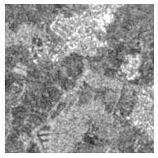
(a) SAR image example, vertical-vertical polarization.

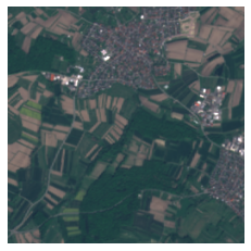
(b) EO image example, RGB.

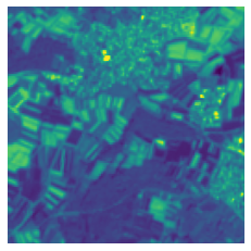
(c) Multi-spectral image example, SWIR band.

Figure 1: Examples of different overhead image modalities from the same scene. From left to right, SAR, EO and multi-spectral.

2.1.1 Electro-Optical Imagery

with this term we refer to satellite images obtained through passive sensors capturing the solar radiations reflected by the Earth’s surface. The first images of this kind were not too dissimilar from natural photographs: they captured light in the visible spectrum thanks to a rigid body camera holding the optics, and a sensor placed directly on the focal plane Toth2016remote . Today’s EO sensors are still optical-based systems, but the technology has progressed to accommodate greater object ground coverage and spatial resolution as required by modern remote sensing systems Toth2016remote .

EO imagery relies mainly on solid-state chip sensors such as Charge-Coupled Devices (CCD) and Complementary Metal-Oxide Semiconductor (CMOS), but in different configuration with respect to those usually employed in consumer photography. Indeed, since the size of such sensors cannot achieve large ground-coverage with a high spatial resolution, they are arranged in linear arrays or area sensors optic on satellites and airborne platforms.

Linear arrays acquire samples with a push-broom modality, i.e., as the platforms moves along its trajectory, long “strips” of pixels, called pixel carpets, are acquired and then “stiched” together to form a single image covering the area of interest. This is the modality adopted, for instance, by Maxar satellites like WorldView2 wv2technical . The second modality, which is employed, for example, by the PlanetLab’s Skysat constellation skysattechnical , relies on one or two-dimensional sensors that do not acquire images as pixel carpets, but as normal frames, i.e., the scene is imaged at the same moment in time with its pixels having the same rigid relationship with respect to each other. Coverage of areas of interest is then obtained by shooting blocks of overlapping photos. In both cases, strong processing follows to provide final users with more manageable data known as products. Examples of processing are radiometric and sensor correction Teillet86image , or orthorectification ortho .

Usually, passive sensors are able to capture wavelengths in the visible spectrum (i.e., Blue light with wavelength around $04\text{\,}\mu\mathrm{m}$) up to Long-Wave Infra-Red (LWIR) (i.e., wavelength up to $20\text{\,}\mu\mathrm{m}$). These wavelengths can be captured either together, or as different channels or bands in the acquired image through the use of high-quality filters, leading to the formation of different kinds of EO products. Panchromatic imagery, for instance, is a monochromatic format of remote sensing data with no spectral information but with high spatial resolution. RGB data collects information in the red, green and blue bands, that are often used, in combination with bands outside the visible spectrum, for discriminating the land-cover content. Finally, Multi-Spectral Imagery (MSI) can be used to collect spectral information up to the LWIR bands divided in 8-15 channels, while Hyper-Spectral Imagery (HSI) can cover the same spectral range but with a higher spectral resolution. HSI can reach up to 100 spectral bands and it is usally employed in more demanding tasks where materials signatures must be accurately identified Harsanyi1994hyperspectral .

2.1.2 Synthetic Aperture Radar (SAR) Imagery

with this term we indicate a remote sensing modality obtained through active sensors, (i.e., imaging radars mounted on moving platforms). As the system travels, it emits sequential high power electromagnetic pulses. These pulses, called chirps, are characterized by constant amplitude and linearly modulated instantaneous frequency. Chirps interact with the Earth’s surface, being reflected as back scattered echoes with amplitude and phase changed according to the characteristics of the objects they hit (e.g., permittivity, geometry, roughness, etc.). The platform receives and collects these echoes, and after a series of processing operations required to make the image interpretable (i.e., focusing Moreira2013 ), a 2D matrix of complex values is returned Moreira2013 . Since the ground coverage of a single echo is often insufficient, SAR images are typically acquired by collecting and concatenating different measurements together in order to cover the whole area of interest. Other processing steps can then follow in order to project the images on the Earth’s surface (e.g., ground-range projection groundrange , orthorectification ortho , etc.).

SAR data has gained a lot of popularity due to the fact that, with respect to EO, is not affected by daylight, weather and cloud coverage conditions Tomiyasu1978 ; Oliver2004 . This makes it suitable for a variety of applications in substitution and/or integrated with EO imagery, such as Earth monitoring, change detection, or Earth surface mapping Moreira2013 .

As with EO imagery, also SAR data is distributed in different formats with different characteristics. Each format is know as a product, and may be useful for different applications. For instance, different frequency bands for modulating the chirps can be used, with the most popular being L (i.e., from 1 GHz to 2 GHz), C (i.e., from 3:75 GHz to 7:5 GHz) and X (i.e., from 7:5 GHz to 12 GHz). Each of them is more suited for different applications, e.g., X for military surveillance, S for medium range meteorological applications, etc Moreira2013 . Other products can also be obtained by further processing the complex 2D matrix. Sentinel-1 Ground Range Detected (GRD) images, whose pixel values approximate the reflectivity of the ground Oliver2004 , is an example of an amplitude-based product.

2.2 Data Sources

The huge increase in the amount and variety of multimedia content shared among people is a phenomenon that also affects remote sensing data. Nowadays, there are many online platforms offering satellite data for free in the form of easy-to-manage products freesat . The purpose of this section is to present some of the most commonly used data collections acquired through popular data acquisition missions and available through different online portals.

2.2.1 Airborne Visible/Infrared Imaging Spectrometer (AVIRIS) Data Portal

AVIRIS refers to an optical sensor realized and operated by NASA that gathers spectral radiance of 224 contiguous visible and Near Infrared (NIR) spectral bands with wavelengths ranging from 400 to $2500\text{\,}\mu\mathrm{m}$ aviris_2022 . The data is gathered using four aircrafts platforms. Until now, the area of coverage is North America, Europe, portion of South America, and Argentina. The AVIRIS project is focused on studies related to climate change and global environment.

2.2.2 Copernicus Open Access Hub

The Copernicus Open Access Hub copernicus is the online portal provided by the European Space Agency (ESA) to download products generated by one of the Sentinel missions. In particular, Sentinel-1 and Sentinel-2 have gained a lot of popularity.

Sentinel-1 mission provides C-band SAR imaging sentinel1_2022 with two satellites, Sentinel-1A and Sentinel-1B, with a revisit frequency of 6 days for both and 12 days for a single satellite. Sentinel-1 images are available through the Copernicus Open Access Hub copernicus in different products. For instance, different acquisition modes (i.e., patterns of movements through which the antenna emits electromagnetic pulses) are available. The simplest one is the Stripmap, where pixel carpets are sensed with a fixed antenna pattern, while a more complex variations is the Interferometric Wide swath (IW), where the system emits three chirps steering the antenna in the platform moving direction. Other differences between products are related to the level of processing they undergo. The Open Access Hub offers them in 3 different levels: level 0 consists of unfocused SAR echo signals; level 1 consists of focused SAR images, provided either as complex signals as Simple Look Complex (SLC) or as amplitude only signals as GRD products; additional levels offer even more processing.

Sentinel-2 mission provides MSI in 13 bands for land monitoring usage sentinelmsi_2022 . As for Sentinel-1, the images ase provided by a pair of twin satellites that has a revisit frequency of 5 days for regular coverage areas. Table 1 shows the spatial resolution of all the multi-spectral bands: 4 bands have a resolution of 10m Ground Sampling Distance (GSD), 6 of 20m GSD, and 3 of 60m GSD. Sentinel-2 MSI is offered in 5 different products, 3 of which are not publicly available (i.e., level-0, level-1A and level-1B). The orthorectified products level-1C (i.e., Top-of-Atmosphere (TOA)) and level-2A (i.e., Bottom-of-Atmosphere (BOA)) are freely available to all users.

Spatial Resolution (m)	Band Number
	2 - Blue
	3 - Green
	4 - Red
10	8 - NIR
	5 - Vegetation Red Edge 1
	6 - Vegetation Red Edge 2
	7 - Vegetation Red Edge 3
	8a - Narrow NIR
	11 - SWIR 1
20	12 - SWIR 2
	1 - Coastal Aerosol
	9 - Water vapour
60	10 - SWIR Cirrus

Table 1: Spatial Resolution of Sentinel-2 MSI bands.

2.2.3 Maxar DigitalGlobe Portal

The DigitalGlobe Discover portal digitalglobe is an online platform for downloading satellite imagery produced by Maxar technologies. Maxar counts 7 satellites in its constellation providing EO imagery, 4 on orbit (i.e., WorldView1-2-3 and GeoEye1) and 3 decommissioned (i.e., QuickBird, Ikonos and WorldView4), whose images, however, are still available in the portal archive. According to the technical guide digitalglobeuserguide , the GSD resolution can vary according to the type of imagery produced: for panchromatic products, the ground resolution varies from $50\text{\,}\mathrm{c}\mathrm{m}$ to $2\text{\,}\mathrm{m}$, while for MSI it ranges from $2\text{\,}$ to $24\text{\,}\mathrm{m}$.

2.2.4 U.S. Geological Survey Landsat Data Access

The United States Geological Survey (USGS) offers a portal usgeologicalysurvey to download all the imagery produced by the Landsat program. The Landsat program landsat is a joint mission by NASA and USGS aiming at monitoring the Earth surface for any remote sensing application, which has been active now for more than 50 years. It comprehends two twin satellites (i.e., Landsat8 and Landsat9) providing MSI in the visible, near and short-wave infrared spectra, as well as thermal infrared wavelengths, with a ground sampling distance of $30\text{\,}\mathrm{m}$.

2.2.5 SEN12MS

The SEN12MS dataset schmitt_2019 is a large scale satellite dataset aimed at training deep learning architectures for land-cover related applications (e.g., land-cover classification, segmentation, etc.). It is made up of 180,662 $256\times 256$ triplets of Sentinel-1 SAR image patches, multispectral Sentinel-2 image patches, and MODIS modis land cover maps. The images span various locations and seasons and have been processed to provide the information related to the same exact location, i.e., to have similar GSD and georeference information. In particular, since Sentinel-2 MSI is orthorectified, Sentinel-1 data has been orthorectified too, while the MODIS land cover maps have been upsampled to reach a resolution of $10\text{\,}\mathrm{m}$ GSD from the original resolution of $500\text{\,}\mathrm{m}$. schmitt_2019
 

3 Generative Models

A GAN goodfellow2014gans architecture provides a game theoretic framework where two networks, namely a generator and a discriminator, are trained in an adversarial manner. Starting from an input noise sample $z$, the generator synthesizes new samples with a distribution $p_{g}$ that is similar to the distribution of some source data $p_{x}$ on which the discriminator is trained. The discriminator analyzes these samples trying to judge whether they are real or synthesized samples produced by the generator. The goal of the generator is to produce samples that can not be distinguished from the real ones by the discriminator. Formally, the generator aims at minimizing the following loss function, i.e., the adversarial loss,

$$\emph{L}_{G}(\Phi_{\text{D}},\Phi_{\text{G}})=\mathbb{E}_{z\sim{p_{z}(z)}}[\log(1-\Phi_{\text{D}}(\Phi_{\text{G}}(z)))],$$ (1)

where $\Phi_{\text{G}}$ is the generator network function and $\Phi_{\text{D}}$ is the discriminator network function. The discriminator’s goal, instead, is to distinguish between generated samples and real ones. Hence, it tries to minimize the following loss function, where $x$ is the input sample, drawn from $p_{x}$:

$$\begin{split}\emph{L}_{D}(\Phi_{\text{D}},\Phi_{\text{G}})={-}&\mathbb{E}_{z\sim{p_{z}(z)}}[\log(1-\Phi_{\text{D}}(\Phi_{\text{G}}(z)))]-\\ &\mathbb{E}_{x\sim{p_{x(x)}}}[\log(\Phi_{\text{D}}(x))],\end{split}$$ (2)

where the first term makes sure that the discriminator recognizes generated samples $\Phi_{\text{G}}(z)$ as such, and the second term makes sure that it recognizes samples $x$ as original ones belonging to $p_{x}$. GANs have been applied successfully to a variety of different domains, from text Yu2017seqgan , to biomedical images Kazeminia2020gans and of course natural images. In particular, a great effort have been paid to continuously improve the quality and realism of synthetic natural images  karras_2017  karras_2018  karras_2019 . Due to the impressive results they got and the high realism of the generated images, many variants of the basic GANs framework were developed, going beyond image generation from scratch, that are widely used in various computer vision tasks, and also for satellite imagery applications. In the following, we describe the most relevant architectures used in the literature.

One of the most relevant GANs-based frameworks is image-to-image translation isola_2016 zhu_2017 , wherein the input image is translated from a semantic domain to another. Image-to-image translation is based on Conditional Generative Adversarial Network (cGAN) Mirza_2014_cgan , an evolution of the basic GAN architecture where the training procedure is modified with the addition of a condition on the inputs of either the generator or the discriminator or both. This condition can derive from any kind of additional information. In isola_2016 , a popular cGAN, named pix2pix is proposed to improve the quality of the generated images. To train the pix2pix architecture, a paired dataset is used where each input image has its corresponding representation in the target domain, namely a reference image $r$ following a distribution $p_{xr}$. For example, if we want to transfer images from summer to winter, we would need images of the same place belonging to both the summer and winter domains where one will act as the input (summer) to be transferred by the generator and the second is the reference that the network will try to simulate from the input. The authors add a term corresponding to the $L1$ distance between the reference images and the generated images, to the loss of the generator, which is now expressed as:

$$\begin{split}\emph{L}_{G}(\Phi_{\text{D}},\Phi_{\text{G}})={}&\mathbb{E}_{x\sim{p_{xr}(x,r)}}[\log(1-\Phi_{\text{D}}(x,\Phi_{\text{G}}(x)))]+\\ &\lambda\mathbb{E}_{xr\sim{p_{xr}(x,r)},}[\left\lVert(r-\Phi_{\text{G}}(x)))\right\rVert_{1}],\end{split}$$ (3)

where $\lambda$ is a weight parameter balancing the importance of the two loss terms $\emph{L}_{D}$ is the same as in (2).

Another very popular cGAN is the Cycle Generative Adversarial Network (CycleGAN) zhu_2017 , whose general architecture is shown in Fig. 2. It replaces the $L1$ distance loss term of pix2pix with a so called cycle consistency loss term, computed by resorting to two generators and two discriminators. The cycle consistency loss is defined as

$$\begin{split}\emph{L}_{cyc}(\Phi_{\text{G}},\Phi_{\text{G2}})={}&\mathbb{E}_{x\sim{p_{x}(x)}}[\left\lVert(\Phi_{\text{G2}}(\Phi_{\text{G}}(x)))-x)\right\rVert_{1}]+\\ &\mathbb{E}_{y\sim{p_{y}(y)}}[\left\lVert(\Phi_{\text{G}}(\Phi_{\text{G2}}(y)))-y))\right\rVert_{1}],\end{split}$$ (4)

where $x$ (drawn from $p_{x}$) denotes a sample from the first domain, given as input to the first generator $\Phi_{\text{G}}$ and the first discriminator ($\Phi_{\text{D}}$), and $y$ (drawn from $p_{y}$) is a sample from the second domain, given as input to the second generator $\Phi_{\text{G2}}$ and the second discriminator ($\Phi_{\text{D2}}$).

An advantage with respect to pix2pix is that with CycleGAN there is no need for a paired dataset for training (that can be difficult, if not impossible, to collect in many applications).

An additional constraint, known as identity loss, can also be added to the loss of the generator. The goal of the identity loss is to ensure that the output of the generator is equal to its input, when a sample $x$ of the first domain is fed at the input of the second generator $\Phi_{\text{G2}}$. The same applies when a sample of the second domain is fed to the first generator $\Phi_{\text{G}}$. Formally, the identity loss has the following expression:

$$\begin{split}\emph{L}_{identity}(\Phi_{\text{G}},\Phi_{\text{G2}})={}&\mathbb{E}_{x\sim{p_{x}(x)}}[\left\lVert(\Phi_{\text{G2}}(x))-x)\right\rVert_{1}]+\\ &\mathbb{E}_{y\sim{p_{y}(y)}}[\left\lVert(\Phi_{\text{G}}(y))-y))\right\rVert_{1}].\end{split}$$ (5)

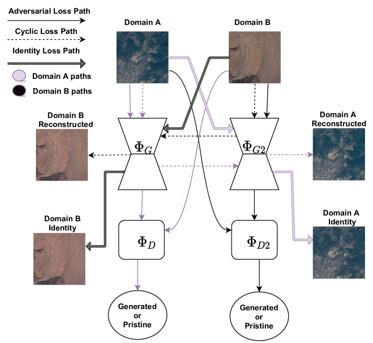
Figure 2: cycleGAN Architecture

Fig. 2 shows the cycleGAN architecture.

A variant of CycleGAN is the No Independent Component for Encoding GAN (NICE-GAN) chen2020 , where, instead of designing a dedicated encoder for the generator, the first layers of the discriminators are used as the generator encoding layers. Hence, the generator and the discriminator share some common layers.

Another line of research aims at improving not only the generated sample quality, but also the training process, to mitigate the problems of convergence instability that often affects GANs. One of the methods proposed to achieve this goal is the Wasserstein GAN with Gradient Penalty loss (WGAN-GP) Gulrajani2017 , where the Wasserstein loss formulation, in which the discriminator acts as a critic and increase the distance between the real and fake samples instead of classifying the images as real or fake, is considered (WGAN arjovsky2017_cwgan ) and a gradient penalty is added to the discriminator’s loss to fulfill a Lipschitz constraint. The loss for the generator and the discriminator are defined as

$$\emph{L}_{G}(\Phi_{\text{D}},\Phi_{\text{G}})=-\mathbb{E}_{z\sim{p_{z}(z)}}[\Phi_{\text{D}}(\Phi_{\text{G}}(z))],$$ (6)

and

$$\begin{split}\emph{L}_{D}(\Phi_{\text{D}},\Phi_{\text{G}})={}&\mathbb{E}_{z\sim{p_{z}(z)}}[\Phi_{\text{D}}(\Phi_{\text{G}}(z))]-\\ &\mathbb{E}_{x\sim{p_{x(x)}}}[\Phi_{\text{D}}(x)]+\\ &\lambda\mathbb{E}_{w\sim{p_{w}(w)}}[(||\nabla_{w}\Phi_{\text{D}}(w)||_{2}-1)^{2}],\end{split}$$ (7)

where $\lambda$ is the gradient penalty tradeoff and $w$ is a random sample either produced by the generator or taken from the distribution of real samples.

Another approach that allows to mitigate the instability of GANs training, to enhance the quality of the generated images, and also to speed up the training, is the progressive training methodology. The main feature of the Progressive Generative Adversarial Network (ProGAN) karras_2017 is the incremental approach, with the size of the model increasing incrementally during training. The training starts on small resolution data, typically $4\times 4$ pixel images, then, during training, additional convolutional layers are added to both the generator model and the discriminator models to increase the resolution.

In addition to GANs, another widely used generation framework builds upon Variational Autoencoders (VAEs) Kingma2014 . An autoencoder Hinton1993_autoencoders A is a neural network trained to reconstruct at the output the same data given as input, after processing it with a series of operations that avoid learning the identity function by respecting some constraints (e.g., reducing the dimensionality of the data at some point in the network). The autoencoder is composed by two blocks:

• the encoder $\emph{A}_{\text{e}}$ that maps the input $x$, to a hidden representation $h$ (i.e., $h=\Phi_{\text{Enc}}(x$)).

• the decoder $\emph{A}_{\text{d}}$ that has a specular architecture compared to the encoder, and that maps the hidden representation to an approximate version of the input $\tilde{x}$ (i.e., $\tilde{x}=\Phi_{\text{Dec}}(h)$).

In case of tensor data, the input can be a RGB image $\mathbf{X}_{\text{RGB}}$ and the hidden representation a vector $\mathbf{h}$, with the encoder and decoder trained together to minimize a reconstruction loss, typically, an L2 loss term, between the input samples and the output (decoded) sample.

In VAEs, the input is not only being encoded into a vectorial representation, but the hidden variable is forced to follow a Gaussian distribution $\mathcal{N}(f(x);g(x))$, with mean $f(\cdot)$ and variance $g(\cdot)$ being functions of the input implemented by the encoder network. At the decoding stage, a sample from the hidden representation variable distribution is drawn and used as input to the decoder which in turn outputs a reconstruction of the initial input data. The main intuition behind this approach is to allow the decoder to generate new data by sampling from the hidden variable distribution. From this perspective, the hidden variable distribution can be assumed to have some desirable properties, e.g., being a Gaussian normal distribution. In this scenario, the total loss iused during training is equal to:

$$\begin{split}\emph{L}(x,\tilde{x})={}&\left\lVert x-\tilde{x}\right\rVert^{2}_{2}+\\ &\beta L_{kl}(\mathcal{N}(f(x),g(x)),\mathcal{N}(0,I_{d})),\end{split}$$ (8)

where the first term represents a “data fidelity term", i.e., a L2 loss between the input sample $x$ and the estimated sample $\tilde{x}$. The second term, applies a kind of “regularization", by forcing the network to minimize the Kullback–Leibler divergence $L_{kl}$ between the learned hidden variable distribution and a desired normal $\mathcal{N}(0;I_{d})$ distribution, with $I_{d}$ being the identity matrix of $d$ dimensionality, and $\beta$ a hyper parameter weight.

After training the VAE, the decoder is used to generate new images by picking random samples from the learned distribution.

4 Satellite Forgeries via Deep Neural Networks

In this section, we overview the most relevant methods for the generation and manipulation of satellite imagery, with particular attention to those based on GANs and VAEs. As mentioned in the introduction, due to the different characteristics of satellite images and to the different needs of remote sensing applications, a number of dedicated methods have been developed, which are suitedfor this kind of images.

In the following, we classify the various methods based on the type of forgery they aim at. In particular, we are considering the following types of forgeries: i) generation from scratch of synthetic satellite images (addressed in Section 4.1) and ii) modification of the semantic content of pre-existing satellite images (Section 4.2).

Table 2 summarizes all the generation methods considered in Section 4 of this overview, categorized according to the proposed classification. Additionally, Figure 3 reports a visual representation of the timeline of the seminal works related to satellite image generation for each datatype.

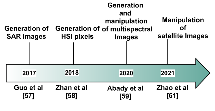
Figure 3: Timeline showing the first satellite generation methods for each datatype

Reference	Year	Task	Data type	Description
Guo2017	2017	Generation from scratch	SAR	Generate simulated SAR images
zhan2018_ganforalignment	2018	Generation from scratch	HSI	Generate HSI to aid later on in classification
abady2020	2020	Generation from scratch	Multispectral	Generate multi-spectral images
abady2020	2020	Semantic Modification	Multispectral	Convert the land cover of multi-spectral images
Ren2021deepfaking	2021	Semantic Modification	Multispectral	Convert the land cover of multi-spectral images
zhao2021_cycleganrgb	2021	Semantic Modification	RGB	Convert the landscape of a source city to that of a target city

Table 2: List of techniques discussed in Section 4 and their characteristics.

4.1 Generation of Synthetic Images from Scratch

In Guo2017 , the authors use a conventional GAN architecture to generate synthetic SAR images. The generator is implemented by a deconvolutional network that takes as input observation parameters, that are directly measured from the images, e.g., platform azimuth and target depression angle, and a latent vector characterizing other observation conditions, that is, the target position and environmental factors such as clouds and rain. The discriminator is fed with real samples and generated ones having the same observation parameters. A cluster normalization procedure is implemented to reduce the influence of the clutter, causing convergence instability. Specifically, segmentation is applied to the images in the training set to separate target and clutter. Then, the images are normalized so that the clutter levels are all the same. Thanks to normalization, the discriminator learns to ignore the clutter and focuses on the target. The generated images are evaluated by applying to them a Convolutional Neural Network (CNN) classifier considering 10 selected target categories from the Moving and Stationary Target Acquisition and Recognition (MSTAR) dataset. The classification accuracy on the synthetic images is similar to that achieved on pristine images, thus proving the plausibility of the synthetic images. The visual quality of the generated SAR images is also assessed and compared with that of images simulated by means of ray tracing raytracing_2010 , and that of real samples, for specific observation parameters. The authors show that both simulators (GAN and ray-tracing) are able to predict images close to real ones.

In zhan2018_ganforalignment , the authors propose a semisupervised algorithm for HSI classification exploiting images produced by GAN s, to overcome the difficulty of gathering a large labeled HSI training dataset. The authors propose a 1D-GAN, called hyper spectral GAN (HSGAN), inspired by the architecture described in radford_2016 (with a difference in the input dimension, set to 1 instead of 2). The proposed framework enables automatic extraction of spectral features needed for HSI classification. The HSGAN is trained by using unlabeled hyperspectral data, so that it learns to generate hyperspectral samples similar to the pristine samples. Once the GAN is trained, the discriminator is modified by replacing the last sigmoid layer with a 16 class sigmoid layer and then is fine-tuned on a small labeled dataset for hyperspectral classification. Both HSGAN training and fine-tuning of the discriminator is performed on the Indian Pines dataset, gathered by AVIRIS sensor in June 1992 over the Indian Pines region in northwestern Indiana. The size of the original images is 145 $\times$ 145 pixels with 220 spectral bands. The noisy and water-absorption bands are filtered out, getting 200 bands, that correspond to the output size of the 1D-GAN.

Fig. 4 shows 128 examples of real and synthetic spectral bands, where each line corresponds to the values assumed by one pixel on the 200 bands. The figure also shows a real and a synthetic waveform. The authors have shown experimentally the superior performance of the HSI classifier trained on synthetic images with respect to state-of-the-art methods. They also assessed the impact of the GAN training dataset size on the classification performance, proving that the size of the HSGAN has a noticeable impact on the classification accuracy; the more data the HSGAN is trained on, the more accurate the classifier is.

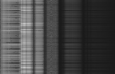
(a) Real Spectral Samples.

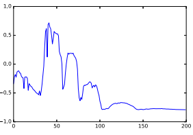
(b) Real Spectral Waveform.

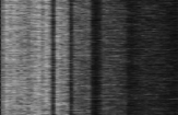
(c) Generated Spectral Samples.

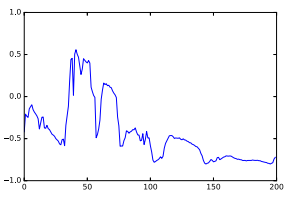
(d) Generated Spectral Waveform.

Figure 4: Examples of real and generated HSI bands from zhan2018_ganforalignment . 4a and 4c show 128 samples of real and generated spectral lines . 4b and 4d show a sample of real and generated spectral waveforms respectively, with 200 values each.

In abady2020 , the authors use a ProGAN architecture karras_2017 to generate 13 bands Sentinel-2 level-1C images of $256\times 256$ resolution. For training, they have used all 180k samples of the SEN12MS dataset. Similar to karras_2017 , a WGAN-GP loss function is used.

4.2 Semantic Modifications

In abady2020 mentioned before, the authors propose an image-to-image translation solution tailored to the remote sensing scenario. They trained a network for land cover transfer, i.e., a network able to change the content of images to move them from one land-cover class to another. In particular, the paper focuses on transferring a sample from the vegetation class into the barren class and vice versa. They rely on the NICE-GAN chen2020 architecture to perform unpaired style transfer. The model was trained on 4 bands, i.e., RGB and NIR (10 meters bands) images of size $480\times 480$ cropped from Sentinel-2 level-1C products, with no cloud coverage. For the vegetation domain, 20k images were gathered from Congo, El Salvador, Montenegro, Gabon and Guyana, while for the barren domain 20k images were gathered from Western Sahara. Samples were split into training and testing. Specifically, 18K images from each domain are used for training, while the remaining 2K are left for testing. Fig. 5 shows an example of real and GAN-transferred images for each transfer direction. The authors also verify that the expected correlation between the bands is preserved in the generated images, by looking at the spectral view of pixels belonging to different land cover classes for both real and generated images.

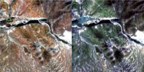
(a) Image translation from barren to vegetation domain.

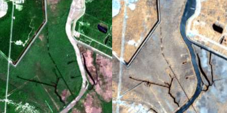
(b) Image translation from vegetation to barren domain.

Figure 5: Land-cover image translation examples taken from abady2020 .

A similar task is pursued by Ren et al in Ren2021deepfaking . In this work, the authors exploit a CycleGAN architecture to translate 10 bands of Sentinel-2 level-1C image, namely the 10m and 20m bands, from drought to vegetation and vice versa.
 

In zhao2021_cycleganrgb , the CycleGAN architecture is used for a different semantic modification: the creation of synthetic images having the urban structure of a given city (i.e., Tacoma in Washington, U.S.) but with the landscape features of another city (i.e., Seattle in Washington, U.S. and Beijing, China). To achieve this task, they train a CycleGAN model on a given city to generate an image with the landscape features of this specific city, starting from an input base-map with the desired city structure. For the map domain, the authors use the cartoDB basemaps, which provides basic urban structural information. As for the satellite imagery domain, they rely on Google Earth’s satellite imagery. They use the QTile plugin in QGIS open source software qgis to collect their datasets for both domains. All datasets have a resolution of $256\times 256$. 1196 pairs of images are collected, that is satellite images and their corresponding basemaps, for Seattle, 1122 pairs for Beijing and 758 pairs for Tacoma. Fig. 6 shows an example of a satellite image generated from a basemap from Tacoma, showing the landscape features of Seattle and Beijing.

Figure 6: An example of generated satellite images using the basemap image in (a) from Tacoma, with the landscape features of Seattle (c) and Beijing (d). (b) shows the ground truth satellite image that belongs to the basemap in (a) zhao2021_cycleganrgb .

5 Beyond Forgeries

In this section, we overview additional methods for the generation and manipulation of satellite imagery, considering techniques proposed to edit an image content without a necessarily malevolent goal. This is the case, for example, of image enhancement techniques. Despite the fact that these methods are not meant to be harmful or used in a deceptive way, they still undermine image integrity to some extent. For instance, a colorized image obtained synthetically from a gray scale one could be considered as altered from the data integrity point of view.

In the following, we consider two types of generation and manipulation: i) generation of satellite images of a given type from a different type of data, e.g., the generation of an EO image starting from a SAR image and vice versa (addressed in Section 5.1); and ii) modifications aiming at quality enhancement, such as colorization and cloud removal (see Section 5.2). Table 3 summarizes all the generation methods considered in this section, categorized according to the proposed classification. Figure 7 shows the timeline of the works described in this section.

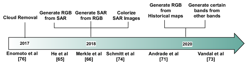
Figure 7: Timeline highlighting the main works related to synthetic image generation that can not be categorized as malevolent forgeries.

Reference	Year	Task	Data type	Description
he2018_rgb	2018	Datatype transfer / Inter-modality	RGB-SAR	Generate optical images from SAR input or fused optical-SAR input
Merkle2018	2018	Datatype transfer / Inter-modality	SAR-RGB	Simulate SAR from optical images
enomoto2018gan	2018	Datatype transfer / Inter-modality	RGB-SAR	Simulate optical images from SAR images
liu2018	2018	Datatype transfer / Inter-modality	RGB-SAR	Simulate optical images from SAR images and vice versa
reyes2019	2019	Datatype transfer / Inter-modality	RGB-SAR	Simulate optical images from SAR images
bermudez2019synthesis	2019	Datatype transfer / Inter-modality	RGB-SAR	Simulate optical images from SAR images
andrade2020	2020	Datatype transfer / Inter-modality	RGB	Generate optical images from historical maps
yuan2020	2020	Datatype transfer / Intra-modality	Multispectral	Generate NIR images from RGB images
vandal2020	2020	Datatype transfer / Intra-modality	Multispectral	Generate certain bands using other bands as input
schmitt2018colorizing	2018	Quality Improvement / Colorization	RGB-SAR	Generate colorized SAR images from SAR-optical fused image
tasar2019	2019	Quality Improvement / Colorization	RGB	Adapt color distribution of a testing dataset to match that of a classifier training dataset
enomoto2017filmy	2017	Qaulity Improvement / Cloud Removal	Multispectral	Remove clouds from RGB images using NIR band as auxiliary information
singh2018	2018	Quality Improvement / Cloud Removal	RGB	Remove clouds from RGB images
grohnfeldt2018_conditional	2018	Quality Improvement / Cloud Removal	Multispectral-SAR	Remove thick clouds from multispectral images
zotov2019	2019	Quality Improvement / Cloud Removal	RGB	Remove clouds from RGB images
ebel2020	2020	Quality Improvement / Cloud Removal	RGB-SAR	Remove clouds from RGB images
gao2020cloud	2020	Quality Improvement / Cloud Removal	RGB-SAR	Remove clouds from RGB images
sarukkai2020cloud	2020	Quality Improvement / Cloud Removal	Multispectral	Remove clouds using temporal data of RGB and NIR bands
wen2021	2021	Quality Improvement / Cloud Removal	RGB	Remove clouds from RGB images

Table 3: List of methods discussed in Section 5 and their characteristics.

5.1 Datatype Transfer

One of the main applications of remote sensing data is Earth monitoring and change analysis. For these tasks, both EO (optical) imagery and SAR are usually exploited, considering data captured at different times. Being able to generate one type of data or modality from the other facilitates these tasks since only a type of data would need to be acquired. We refer to this kind of image translation with the term inter-modality datatype transfer. As described in Section 5.1.1, several methods have been proposed in this category.

Another remote sensing application for datatype transfer comes from land cover classification and object detection. Typically, different spectral bands are used for these tasks. Instead of incurring in the costs of acquiring all the bands, only some of them are acquired while the others are synthetized automatically. Similarly, we can generate missing spectral bands relying on existing spectral bands. We refer to this kind of transfer as intra-modality datatype transfer (Section 5.1.2).

5.1.1 Inter-modality Transfer

the prediction of optical images using SAR images is first considered in he2018_rgb ,

Specifically, he2018_rgb addresses the problem of generating optical images that represent a prediction of the foreseen land-cover changes using different combinations of remote sensing data as input. Two different architectures are proposed. The best performing method resorts to a pix2pix architecture, that adopts a ResNet-like architecture He2016resnet for the generator, and a patchGAN isola_2016 with 5 layers for the discriminator. The patchGAN classifies the patches of an input image, providing a score matrix at the output; the final score on the whole image is taken by the discriminator by averaging all the outputs.

Let T1 be a given acquisition time or period, and T2 the target period (corresponding to a later time - the images are considered of the same period if the collection dates’ difference is less than 5 days). Two combinations of the input samples are considered in he2018_rgb and their impact on the networks’ ability to predict the optical samples assessed. Specifically, the authors consider providing as input: i) only SAR images, from both T1 and T2; ii) both SAR and optical images from T1 and SAR images from T2. In the following, the two networks trained with the two input combinations will be denoted as cGAN and MTcGAN, respectively.

The data for training and testing are gathered from the Copernicus hub copernicus . Three different regions are considered for the experiments: Iraq, Jianghan, and Xiangyang. For each area, 4 images are downloaded from the Copernicus hub, that is two Sentinel-1 images (i.e., SAR) and two Sentinel-2 images (i.e., EO), from T1 and T2. SAR images were pre-processed using Sentinel Application Platform (SNAP). For Sentinel-2 products, only 4 bands are considered, i.e., RGB and NIR, with a GSD of $10\text{\,}\mathrm{m}$. The SAR and optical images are co-registered by reprojection in order to provide information on the same geographical area. Then the images were divided into $256\times 256$ patches and split into training and test sets.

With the assessment made in he2018_rgb , it is argued that using the optical data as additional input is beneficial, leading to an improvement of the networks’ capability of predicting the optical samples corresponding to T2.

Inspired by he2018_rgb , considerable research has been dedicated to the generation of optical images from SAR images and vice versa, for a different or also the same acquisition time. The most relevant approaches are described in the following.

The opposite transfer with respect to that considered in he2018_rgb , that is, the generation of SAR images from optical images, is addressed in Merkle2018 , with the goal of improving the matching between optical and SAR images, to improve the geolocation accuracy of optical satellite images. The authors use a pix2pix architecture to generate SAR patches from the corresponding optical image using three different losses: the original GAN loss, a variation of the adversarial loss adopting the mean square error in place of the log likelihood mao2017_lsgan , and finally the conditional Wasserstein loss arjovsky2017_cwgan . Training is performed on 201 $\times$ 201 paired patches from TerraSAR-X (SAR) and PRISM (optical), gathered all over Europe.

Finally, they assess the matching between the SAR images and the generated SAR images using three SOTA image-matching techniques: Normalized cross-correlation (NCC), Scale Invariant Feature Transform (SIFT) and Binary Robust Invariant Scalable Key (BRISK). All metrics prove that the generated SAR images were beneficial to improve the matching.

Other methods have been proposed addressing similar tasks. In enomoto2018gan , the pix2pix architecture is used to address the transfer from SAR images to optical images. A CycleGAN architecture, instead of a pix2pix, is used in reyes2019 for the same task of translating SAR into optical images. In liu2018 , a CycleGAN architecture is proposed to perform both translation, from optical to SAR images, and vice versa. Finally, in bermudez2019synthesis , the authors address the generation of optical images from SAR images at different times, to mitigate the impact of heavy clouds on optical images (i.e., generating optical images that do not contain clouds). The same approach introduced in he2018_rgb is used, with the difference that a pix2pix archiutecture is considered instead of the cGAN architecture that is adopted in he2018_rgb .

A last application of inter-modality transfer is the generation of optical images starting from maps or auxiliary raster data. In andrade2020 , the authors generate satellite-like imagery from historical maps using a pix2pix network. They train the pix2pix architecture on satellite images extracted from Google and the corresponding segmented images, providing the optical image and the segmented image as input images from the two domains. During testing, segmentation is applied to the historical maps, then the generator is fed with the segmented image to get the optical image representing the area (what the area might have looked like). They train two models, one on urban areas and the second on rural and natural areas. They argue that merging the output of the two models based on the label (that is, taking the urban labeled pixels from the model trained on urban area, and the rural labels from the model trained on rural areas) yields a better representation of the area.

In baier2022synthesis , the authors generate optical RGB and SAR imagery from land cover segmentation maps and auxiliary raster data, To this purpose, they use a variation of the pix2pix architecture where all the normalization layers are replaced by spatially adaptive normalization (SPADE) layers spade_2019 . The auxiliary data is used as an input to the generator while the land cover is passed as an input to all SPADE layers. For training and testing, two datasets are used: i) GeoNRW geonrw_2020 , containing aerial photographs, terraSAR-X, DEMs and land cover with 10 classes; ii) DFC2020 DFC_2020 , containing Sentinel-1, Sentinel-2 and land cover data with 10 classes. For the GeoNRW, SAR images or optical images is generated from land cover maps and Digital Elevation Models (DEM) dem_2021 used as auxiliary data, while for the DFC2020 (that lacks DEM data), SAR and optical imagery are generated using either solely land cover maps or a combination of land cover with optical (for SAR generation) or SAR imagery (for optical generation) as auxiliary input. To judge the effectiveness of the generation in terms of land cover coverage, the authors analyze the land cover segmentation maps obtained by a U-Net trained on real data and compare the land cover map obtained from the generated images with the ground truth map, that is used for the generation. The results show that the generated images are comparable to the real images in term of land cover maps. Moreover, the authors show that this type of image-to-image translation can also be used to modify the semantic content of an image. For instance, by applying a threshold to a certain height in the DEM image, and modifying the pixels of the land cover map with a value in the DEM image below that height and labeling them as water, we can get a modified image with a larger area covered by water. An example of this semantic modification obtained with the transfer network in baier2022synthesis is shown in Fig. 8.

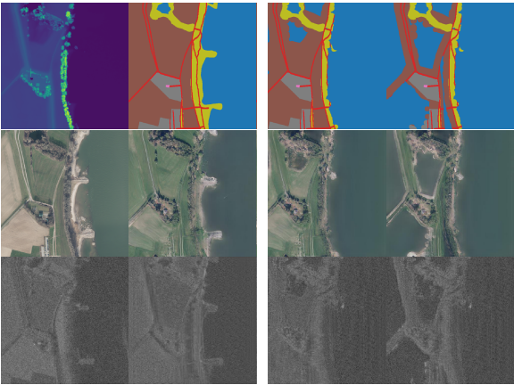
Figure 8: An example of generated datatype with semantic modification baier2022synthesis . The first column shows a real DEM, optical and SAR image. The second column shows the original land cover map with the corresponding generated optical and SAR image. The third and fourth column show the modified land cover with threshold set to height 32m and 33m respectively with the corresponding generated optical and SAR images.

5.1.2 Intra-modality Transfer

A different kind of datatype transfer regards the generation of a subset of EO bands starting from a different subset of bands. In yuan2020 , the authors resort to a pix2pix network for generating the NIR band of Sentinel-2 samples using the RGB bands as input. The model is trained using a subset of SEN12MS dataset.

In vandal2020 , the authors synthesize multiple spectral bands from other bands, using unsupervised image-to-image transfer liu2017_unsupvaegan . More specifically, they rely on a VAE-GAN, that is a combination between a VAE and a GAN, proposed in Larsen_2016 , where a discriminator is used to learn to differentiate between VAE output and real samples, and is used in an adversarial fashion to improve the reconstruction error of the VAE. To improve the reconstruction, the authors introduce skip connections in the network and a shared spectral reconstruction loss, encouraging the decoder to reconstruct identical spectral wavelengths with similar distributions while still synthesizing dissimilar bands. The shared reconstruction loss exploits the availability of shared spectral bands from different satellites. Data for training and testing are gathered from 3 geostationary satellites: GOES-16, GOES-17, and Himawari-8, with 16 spectral bands, 15 of which overlap, with similar information content (GOES-16 and GOES-17 include two visible -blue, red-, four near-infrared -including cirrus-, and ten thermal infrared bands. H8 captures three visible -blue, green, red-, three near-infrared -missing cirrus band -, and the same ten thermal infrared bands as GOES-16 and GOES-17). The authors first evaluate the ability of the network to generate an individual band from the other 15 bands acquired by the same satellite and the full set of bands from the other two satellites. This approach is applied to GOES-16, hence each model takes 15 bands of GOES-16 and 16 of GOES-17 and Himawari-8. The improvement in the reconstruction error brought by the modifications introduced by the authors, with respect to the use of a standard VAE, is proven experimentally. The reconstruction mean absolute error (MAE) obtained with the proposed solution is then compared against the use of cross sensor and UNIT unit_2017 as a baseline proving the superior performance of the proposed method in terms of MAE and precision. They also assess the capability of the network to generate multiple missing bands from satellites with a limited number of spectral bands (older generation satellites often have fewer channels hence being able to generate additional frequency bands can be very useful). Models are trained on GOES-16, removing bands one by one until just one band was left, and reconstructing the missing bands. All 16 GOES-17 and Himawari-8 bands were kept. They observe that the reconstruction MAE decreases monotonically (approximately) as more bands are given as inputs. These results show that few bands (3-4) are needed to synthesize images with an acceptable MAE.

5.2 Quality Improvement

Editing remote sensing images using deep learning is not confined to changes in the semantic content or in the datatype. Methods have also been developed to change the properties of the image itself, e.g., performing colorization or reduction of cloud coverage.

5.2.1 Colorization

Being unaffected by weather and daylight conditions, SAR images are a valuable asset in many applications. However, with respect to EO imagery, SAR images are more difficult to interpret visually, as the frequency range they capture does not cover the visible part of the spectrum. For this reason, an explored research topic in the remote sensing community is the colorization of SAR images, i.e., the fusion of information from SAR and EO imagery, through the use of matching image pairs.

Recently, the use of DNN for colorizing SAR images has been investigated. In schmitt2018colorizing , the authors propose to colorize SAR images by means of an architecture derived from deshpande2017_imgclr , which encompasses a VAE along with a mixture density network (MDN) bishop94_mixturedensity . They first train the VAE to learn low dimensional embeddings of images obtained by fusing SAR and optical images through color space transform pauli_77 . Then, they train MDN to learn the relationship between the original grey-scale SAR image and the low dimensional latent variable embedding of the corresponding SAR-optical fused image generated by the VAE. During testing, given a SAR image as input, the low dimensional latent variable embedding of the SAR-optical fused image is obtained from the MDN, and is then forwarded to the decoder of the VAE to get the final colorized SAR image. Fig. 9 shows a couple of examples of the SAR input image, the desired optical-SAR fused image, the optical image and the synthetic colorized SAR image.

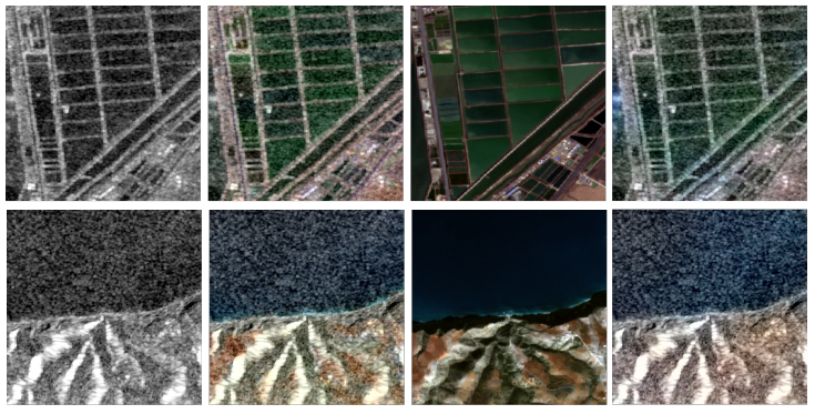
Figure 9: Examples of SAR image (left column), target fused optical-sar image (second column), corresponding optical image (third column), and generated colored example (right column) schmitt2018colorizing

Another application of image colorization considers the correction of EO images to mitigate the effect of acquisition conditions (e.g., atmospheric effects). This problem affects the generalization capability of deep learning tools based on the semantic content, given that training and testing datasets might present different distributions of the spectral bands values because of different acquisition conditions. For instance, very often there exists a large difference between spectral bands of satellite images collected from different geographic locations. To overcome the impact of spectral distribution diversity due to acquisition conditions, in tasar2019 , the authors propose a new GAN, named ColorMapGAN, able to generate images semantically identical to the images in the training dataset, but with spectral distribution similar to the test dataset. To preserve the exact semantics, the authors avoided the use of convolutional and pooling layers, that are part of traditional CNN-based GAN architectures. Instead, ColorMapGAN simply transforms the colors of the training images into the colors of the test images without introducing any structural changes on the objects of the training images. The colorMapGAN is then used to finetune semantic classifiers by generating samples whose spectral distribution targets that of a desired testing dataset.

5.2.2 Cloud Removal

Another common quality improvement to reduce the impact of atmospheric conditions in the acquired images is the removal of clouds from EO images. This problem has been addressed in many works.

In enomoto2017filmy , the authors propose to use a pix2pix architecture to remove thin clouds from images. They consider the RGB bands and the NIR band as input, where the NIR band is regarded to as additional (auxiliary) information provided to the network. The cloud-free RGB image and a binary mask, indicating the cloudy pixels in the original input image, are returned as output. Due to the difficulty of gathering paired images of the same location with and without clouds, the cloud coverage is simulated using Perlin noise perlin2002_noise and then merged into the RGB image by alpha blending to get the synthetized cloudy image. Finally, color correction is applied to both classes of images (i.e., images free of clouds and not) to improve the quality of the images. The network is trained on images gathered from WorldView2, where the RGB bands and the NIR band are used as a multi-spectral input, and the $L1$ loss is computed between the 4-dim output (consisting of the generated cloud-free RGB images and the cloud mask), and the corresponding ground truth (the real RGB image with no clouds and the ground truth mask of cloudy pixels). Fig. 10 shows some examples of generated cloud-free RGB image and the generated cloud mask.

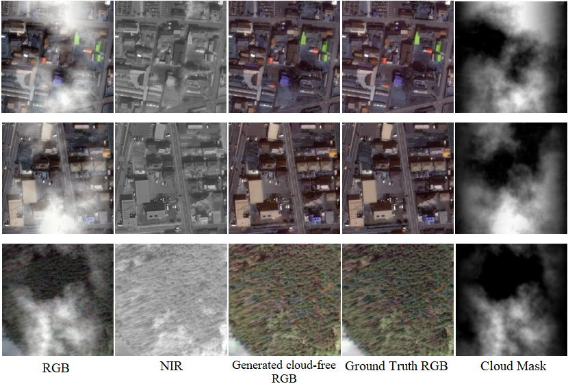
Figure 10: Some examples obtained by the cloud removal method in enomoto2017filmy . From left to right: input cloudy RGB images, the corresponding NIR band, the generated cloud-free RGB images, the ground truth RGB images with no clouds, and finally the generated cloud mask.

Several methods have been proposed to extend enomoto2017filmy . In wang2019 the authors propose to use a novel objective function to train the pix2pix network, to the purpose of improving the quality of the generated cloud-free images. In singh2018 , the authors propose to substitute the pix2pix architecture with a CycleGAN to avoid the need for a paired dataset. In this way it is possible to use real cloudy images instead of synthesized cloudy images for training the GAN. Moreover, only RGB bands are considered, without the need of auxiliary information. A similar approach is followed in zotov2019 .

Later works performing cloud removals with GANs focus on the generation of different spectral bands, using different data types as auxiliary input data. In grohnfeldt2018_conditional , the authors resort to the same pix2pix architecture and the clouds synthesis procedure described in enomoto2017filmy , to train a GAN on 10 bands of Sentinel-2 level-1C images, i.e., the bands with $10\text{\,}\mathrm{m}$ and $20\text{\,}\mathrm{m}$ GSD, and are used the SAR images as additional input. Relying on SAR instead of just NIR as auxiliary information, they are able to remove also thick clouds and dehaze the image.

Another work where SAR images are used as auxiliary information for the generation of cloud-free optical images is ebel2020 . The only difference between this work and grohnfeldt2018_conditional is that a cycleGAN is adopted, instead of pix2pix, to avoid the need of a paired dataset. In gao2020cloud , the authors propose to further improve declouding of optical images by exploiting datatype transfer Specifically, they first transfer from SAR to optical images. Then, a GAN is used to fuse the simulated optical image, the SAR image and the optical image corrupted by clouds. The simulated optical image provides the reference for the cloudy pixels. Fusion allows to inject accurate spectral information and high-frequency texture in the cloudy area.

Other works focused on the use of more complicated network architectures and training procedures. For instance, in sarukkai2020cloud , the authors propose a GAN that exploits temporal sequences of cloudy images, namely Spatio-Temporal Generative Adversarial Network (STGAN). Training is performed on a dataset of RGB and NIR bands extracted from Sentinel-2 examples. A temporal sequence of three cloudy images is considered as an input, with a cloud-free image used as reference. The three cloudy images and the cloud-free image are captured from the same location at different times. The proposed STGAN rely on a PatchGAN discriminator. For the generator, two architectures have been considered, a branched ResNet-based and branched U-Net based architecture. The branched ResNet processes each of the three cloudy image through a separate encoder-decoder. Then, the output features from the three branches are concatenated in pairs, and each pair is fed into another encoder-decoder; the outputs of the second block of encoders-decoders are concatenated into one vector that is fed as input to a last encoder-decoder block. The architecture of the branched ResNet generator is illustrated in Fig. 11.

Figure 11: Branched Resnet Architecture in sarukkai2020cloud .

The U-Net, instead, processes each image in the input sequence through a separate encoder, and then all the outputs of the encoders are concatenated and fed to a single decoder.

The proposed solution is compared against the baseline method in enomoto2017filmy . The results shown in sarukkai2020cloud prove that, when using either branched Resnet or branched U-Net, STGAN provides better quality for the final generated cloud-free images (slightly better results are obtained when using the branched ResNet). In addition, it is shown that the cloud-free images generated using STGAN can also help for land cover classification, as classification works better with STGAN generated cloud-free images with respect to the use of original cloudy images, or cloud-free images generated with the baseline method.

Finally, in wen2021 , the authors improve the results of enomoto2017filmy in terms of quality of the generated images considering the YUV color space for the input, instead of the RGB, treating luminance and chroma components independently. As a further difference with respect to enomoto2017filmy , they resort to a WGAN arjovsky2017_cwgan architecture which is trained in two-steps. A first training is performed on cloud-free and synthetic cloudy images. Then, the model is fine tuned on pairs of cloud-free and real cloudy images, thus avoiding training from scratch on a limited dataset. This two-steps training process allows to get better performance in data scarcity conditions, when a limited set of acquired cloud-free and cloudy images for the same locations are available.

6 Forgery Detection and Localization

In this section, we consider satellite image forensic methods for the detection of synthetic media and the localization of manipulations. We are interested in both the recognition of DNN-generated contents (referred to as synthetic forgeries), being them an entire overhead image or just some regions of it, as well as in the identification of satellite images that have been manipulated with the help of common editing tools (i.e., Photoshop, GIMP, etc.) starting from genuine images. In fact, while the emergence of applications of AI-tools for editing overhead imagery is worrying the community maliciousOverheadAI , malicious modifications created with general purpose softwares like Photoshop are still a non-negligible threat. As a matter of fact, many satellite products are provided in formats easy to use and manipulate (e.g., GeoTIFF, JPEG, etc.). This element, together with the facility of use of editing software suites, allows even non-expert users to create credible forgeries, that can be used for instance to create misinformation campaigns australia_wildfire .

To tackle with these menaces, the main idea behind most forensic methods is to exploit the concept of data life-cycle: during the existence of a multimedia object, various non-invertible operations are executed, each of them leaving a peculiar footprint that can be exploited to reconstruct the chain of operations the object has undergone. Forensic methods use this knowledge to expose malicious editing operations or to understand whether an image is authentic or it has been artificially synthentized.

The life-cycle of satellite imagery is characterized by a processing chain completely different from that of natural photographs, including the type of sensors and modalities used for their acquisition optic , as well as the compression schemes used to encode them. Also the editing needed for making them manageable by final users (e.g., orthorectification ortho , radiometric correction, etc.) includes operations that are very specific to the satellite context. All these reasons have pushed the multimedia forensic community to develop techniques specifically tailored to satellite data analysis.

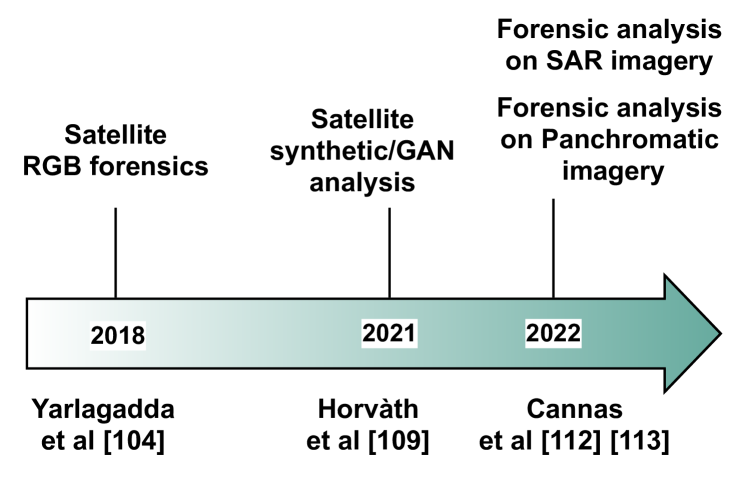
Figure 14: Timeline reporting the first forensic techniques for each datatype

In the following, we first provide some formal definition common to forensic detection and localization methods. Then, we overview the forensic techniques reported in Table 4, grouping them into two categories: i) methods explicitly developed for synthetic image detection and localization; ii) methods for forgery detection and localization that, despite they can in principle be used also to spot synthetic content, are targeted to more general overhead imagery manipulations. Figure 14 highlights the timeline of the initial works related to each datatype.

Table 5 provides some information about the datasets used by the various forensic detectors and their performance. Note that papers tend to use ad-hoc datasets, thus making it difficult to directly compare the reported results. The metrics used for detection are those typically used to evaluate binary classifiers: ROC-AUC fawcett_2006 (i.e., the area under the receiver operating characteristic curve) ; F1-score taha_2015 (i.e., the harmonic mean between precision and recall); Accuracy (i.e., the degree of closeness of the obtained answers to their actual value). In addition to these metrics, localization performance are evaluated also in terms of: PR-AUC he_2013 (i.e., the area under the precision-recall curve); Jaccard Index (JI) manning_2001 (i.e., the ratio between the number of correctly detected forged pixels and the number of pixels in the union set between actual and detected forged pixels).

Reference	Year	Kind of data	Goal	Description
yarlagadda2018satellite	2018	Color optical images	Detect and localize splicings	One-class GAN autoencoder as feature extractor followede by one-class SVM
bartusiak2019splicing	2019	Color optical images	Detect and localize splicings	Conditional GAN is trained on two classes. Generator is used to estimate masks
horvath2019anomaly	2019	Color optical images	Detect and localize splicings	Jointly trained autoencoder and one-class SVM
masmontserrat2020generative	2020	Color optical images	Localize splicings	Use ensemble of PixelCNNs to estimate heatmaps from images
horvath2020manipulation	2020	Color optical images	Detect and localize splicings	One-class DBN for detection and localization
horvath2021_visiontransformer4detection	2021	Color optical images	Localize splicings	Visual Transformer used to reconstruct image. Binary mask obtained through input-output difference
horvath2021_attentionunet	2021	Color optical images	Detect and localize GAN-based inpainting	Nested U-net trained to estimate heatmaps
chen2021_geodefakehop	2021	Color optical images	Detect synthetic images	Subspace learning for fake image detection
zhao2021_cycleganrgb	2021	Color optical images	Detect synthetic images	Hand-crafted features and Support Vector Machine (SVM) to detect GAN-generated images
Ren2021deepfaking	2021	Multispectral images	Detect synthetic images	Binary CNN
cannas2022amplitude	2022	SAR amplitude images	Localize splicings	Extracted noise pattern fed to supervised or unsupervised segmentation methods
cannas2022panchromatic	2022	Panchromatic images	Copy-paste localization	Ensemble of attribution CNNs

Table 4: List of forensics detectors and their characteristics.

Reference	Dataset	Performance - Detection	Performance - Localization
yarlagadda2018satellite	Ad-hoc spliced samples created on purpose using Landsat RGB images	$\text{ROC-AUC}=89.6\%$	$\text{PR-AUC}=11.7\%$
bartusiak2019splicing	Ad-hoc spliced samples created on purpose using Landsat RGB images	$\text{ROC-AUC}=100\%$	$\text{PR-AUC}=95.3\%$
horvath2019anomaly	Ad-hoc spliced samples created on purpose using Sentinel-2 RGB images	$\text{ROC-AUC}=96.6\%$	$\text{PR-AUC}=21.9\%$
masmontserrat2020generative	Ad-hoc spliced samples created on purpose using Sentinel-2 RGB images	n/a	$\text{PR-AUC}=59.9\%$
horvath2020manipulation	Ad-hoc spliced samples created on purpose using Sentinel-2 RGB images	$\text{ROC-AUC}=77.4\%$	$\text{PR-AUC}=28.4\%$
horvath2021_visiontransformer4detection	Ad-hoc spliced samples created on purpose using DigitalGlobe and PlanetScope RGB images	n/a	$\text{F1-score}=0.36$, $\text{JI}=0.275$
horvath2021_attentionunet	Ad-hoc spliced samples created on purpose using generated content by several GANs trained on Sentinel-2 RGB images	$\text{ROC-AUC in SD scenario}=91.8\%$ $\text{ROC-AUC in CD scenario}=66.7\%$	$\text{JI in SD scenario}=73.5\%$ $\text{JI in CD scenario}=0.21\%$
chen2021_geodefakehop	Synthetic samples created using different GANs trained on Google’s Earth and CartoDB RGB images	$\text{F1-score}=100\%$	n/a
zhao2021_cycleganrgb	Synthetic samples created using different GANs trained on Google’s Earth and CartoDB RGB images	$\text{F1-score}=95.3\%$	n/a
Ren2021deepfaking	Synthetic samples created using Sentinel-2 MSI	$\text{Accuracy}=100\%$	n/a
cannas2022amplitude	Ad-hoc spliced samples created on purpose using Sentinel-1 SAR images	n/a	$\text{Mean JI}=0.674$
cannas2022panchromatic	Ad-hoc spliced samples created on purpose using DigitalGlobe panchromatic images	n/a	$\text{ROC-AUC}=85.7\%$

Table 5: List of datasets used and average performances of the forensic detectors. Results not available in the original papers are denoted with ‘n/a’. For horvath2021_attentionunet , ROC-AUC values are averaged, and SD and CD indicate respectively the same dataset and cross dataset scenarios. JI represents the Jaccard Index.

6.1 Forensic detectors definitions

The forensic analysis of overhead images can be carried out with two different goals in mind: i) detection, and ii) localization. Under the detection assumption, the analyst is interested in estimating the likelihood that the image under analysis has been tampered with (partly or completely). With localization, the analyst is interested in estimating which region of an image has been manipulated.

Formally, let us define a generic satellite image with $U\times V$ pixel resolution as $\mathbf{X}$. The coordinates of its pixels can be represented as $(u,v)$, where $u\in[1,\dots,U]$ and $v\in[1,\dots,V]$. $U$ and $V$ are the number of rows and columns, respectively. The pixel-by-pixel integrity of the image can be defined by a tampering mask $\mathbf{M}$, with the same resolution of $\mathbf{X}$, whose pixels take a binary value 1 or 0 depending on whether the corresponding pixel has been manipulated or not. More formally

$$\mathbf{M}(u,v)=\begin{cases}1,\quad\text{if $(u,v)\in\mathcal{S}$}\\ 0,\quad\mathrm{otherwise}\end{cases},$$ (9)

where $\mathcal{S}$ denotes the manipulated region. Given an image $\mathbf{X}$, we can attribute to it a binary label $y$ of value $0$ if $\mathbf{X}$ is pristine, and $1$ if it contains manipulated content. Figure 12 provides an example of manipulations executed on different modalities of satellite data.

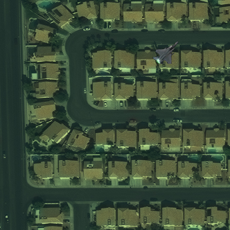
(a) Manipulated $\mathbf{X}_{\text{RGB}}$.

(b) Tampering mask $\mathbf{M}_{\text{RGB}}$.

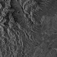
(c) Manipulated $\mathbf{X}_{\text{SAR}}$.

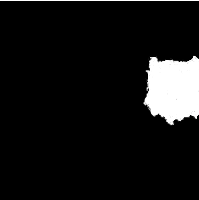
(d) Tampering mask $\mathbf{M}_{\text{SAR}}$.

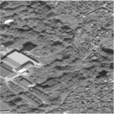
(e) Manipulated $\mathbf{X}_{\text{Pan}}$.

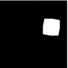
(f) Tampering mask $\mathbf{M}_{\text{Pan}}$.

Figure 12: Examples of manipulated satellite images from different modalities, together with their tampering mask indicating the attacked area. On top row, RGB data from yarlagadda2018satellite ; in the middle, SAR from cannas2022amplitude ; at the bottom, panchromatic from cannas2022panchromatic .

In this framework, detecting if an image has been manipulated consists in designing a detector that implements a function $d(\mathbf{X})$ returning a soft forgery score $\tilde{y}$ (i.e., the likelihood that $y=1$) or a hard forgery score $\hat{y}$ (i.e., an estimate of $y$). Localizing a forgery consists in either estimating a soft tampering mask $\tilde{\mathbf{M}}$ (i.e., the pixel-by-pixel likelihood that each pixel has been forged) or a hard tampering mask $\hat{\mathbf{M}}$ (i.e., an estimate of $\mathbf{M}$). An example of a soft and hard mask is reported in Figure 13.

(a) Spliced $\mathbf{X}_{\text{Pan}}$.

(b) Ground truth tampering mask $\mathbf{M}_{\text{Pan}}$.

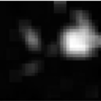
(c) Soft tampering mask $\tilde{\mathbf{M}}_{\text{Pan}}$.

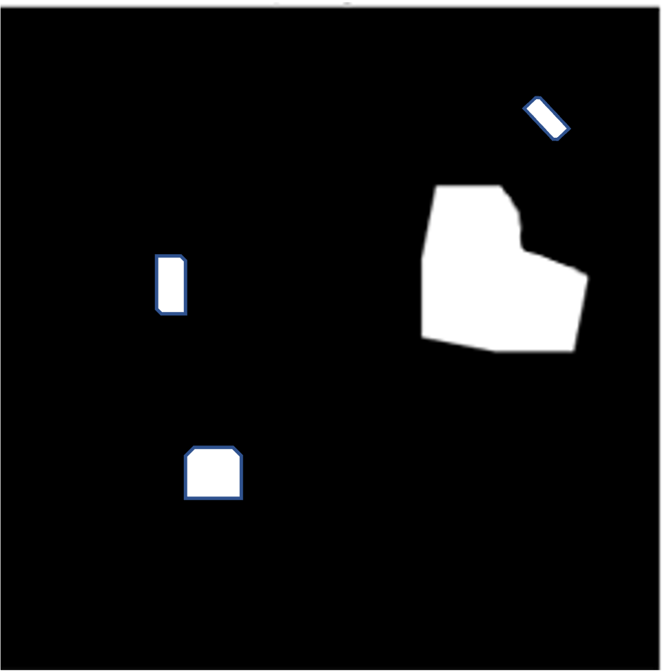
(d) Hard tampering mask $\hat{\mathbf{M}}_{\text{Pan}}$.

Figure 13: Examples of soft $\tilde{\mathbf{M}}$ and hard $\hat{\mathbf{M}}$ tampering masks obtained from a spliced panchromatic sample presented in cannas2022panchromatic .

6.2 Synthetic image detection and localization

Section 4 has shown that it is possible to generate high-quality synthetic satellite images. As it happened with other types of artificial data (e.g., synthetic images of faces, animals, etc.), concerns regarding the possible malicious usage of these generators are raising.

This section deals with the detection and localization of forgeries generated through synthetic satellite image generation tools. For this kind of forgeries, the majority of forensics tools rely on data-driven techniques. This is partly motivated not only by the complex processing pipeline characterizing satellite imagery, but also by the fact that the forensic traces contained in forgeries generated through neural networks are not easy to model. A common approach consists therefore in training specialized CNNs for detecting and localizing synthetic forgeries.

In horvath2021_attentionunet , the authors localize RGB forgeries generated by 3 different families of GANs: StyleGAN2; ProGAN; CycleGAN. More specifically, the authors have generated a dataset of Sentinel-2 RGB images splicing them with each one of the analyzed GANs. Their approach is based on a modified version of a CNN used for image segmentation called Nested Attention U-Net (NAU-N). This network takes as input a $\mathbf{X}_{\text{RGB}}$ image and outputs directly a soft mask $\tilde{\mathbf{M}}$ with each pixel value indicating the likelihood that the pixel has been generated by one of the analyzed GANs.

Being a data-driven method, the NAU-N needs to be trained directly on synthetically spliced samples. Nevertheless, the authors demonstrate the feasibility of their solution in a cross-dataset scenario, i.e., training the NAU-N on images spliced with a specific type of GAN and testing it on images generated by a GAN which was not included in the training set.

In zhao2021_cycleganrgb , the authors not only present a GAN-based approach for semantic satellite image translation, but also provide a data-driven approach for detecting the synthetically generated images. As a matter of fact, they rely on SVMs trained with a number of features (i.e., spatial, histogram-based and spectral features plus a combinations of the three) to detect CycleGAN generated images.

Using the same dataset presented by Zhao et al. zhao2021_cycleganrgb , in chen2021_geodefakehop Chen et al. provide another data-driven method to detect semantically translated RGB satellite images. The core concept is based on the assumption that GANs have difficulties in creating high-frequency details in generated samples. They therefore analyze an input $\mathbf{X}_{\text{RGB}}$ image dividing it into several patches, and perform a frequency analysis using a filter-bank named Subspace Approximation with Adjusted Bias (SAAB) transform. Coefficients from each filter are first used to train a XGBoost chen2016xgboost classifier learning patch by patch the most discriminant frequency coefficients. Then, coefficients from all patches are considered as features for taking a global decision regarding the authenticity of the analyzed sample.

Finally, in Ren2021deepfaking Ren et al. rely on a simple CNN to detect season transferred multi-spectral images generated through CycleGANs. In their study they reach very good detection performances, even though one of their major findings consists in the fact that relying on a simple CNN exposes the detection process to adversarial attacks. However, they have showed that adversarial training can make such a simple approach effective in distinguishing synthetically generated images. They also provide some insights about the features that a CNN-based classifier finds more useful in the classification of GAN-generated multispectral images, thanks to the use of gradient-interpretability techniques such as Integrated Gradients Sundararajan2017axiomatic .

6.3 Forgery detection and localization

The literature on methods explicitly focusing on the detection of synthetic forgeries is rather limited. However, synthetically generated content can in principle be treated as a specific kind of local or global forgery. It is therefore possible to exploit general purpose satellite image forgery detectors to also expose synthetic forgeries. Indeed, image forgery detection consists in understanding if the image under analysis has been edited (in part or in its totality according to some specific editing definition) or not. Image forgery localization consists in understanding which pixels of the image under analysis have been edited (if any). Editing may be a splicing operation, as well as the insertion of synthetically generated content.

Current image forensics SOTA solutions for forgery detection and localization rely on the use of data-driven solutions Verdoliva2018deep . Not surprisingly, this trend also applies to satellite images. As a matter of fact, data-driven techniques enable automatic extraction of meaningful forensics features from corpora of data. In this way, it is possible to devise a good solution also in situations in which data models may be complex or uncertain (e.g., due to the wide variety of possible satellite products).

In this section, we analyze the SOTA data-driven forensics solutions developed for the tasks of forgery detection and localization in satellite imagery. In the following, we organize the discussion about forgery detection and localization methods based on the modality of satellite imagery analyzed by the considered techniques: i) RGB images; ii) panchromatic images; iii) SAR images.

6.3.1 RGB images

In yarlagadda2018satellite Yarlagadda et al. tackle the problem of detecting and localizing general image manipulations on RGB satellite images as an anomaly detection task. More specifically, their approach consists in the training of a CNN as an autoencoder.

As introduced in Section 3, autoencoders are a particular kind of Neural Networks (NNs) whose goal is to reconstruct at the output the data provided as input. While this procedure may seem trivial, training of the autoencoder A in yarlagadda2018satellite is performed in such a way that the hidden representation vector $\mathbf{h}$ possesses some desirable properties. Indeed, the dimension of $\mathbf{h}$ is forced to be considerably smaller than that of the input $\mathbf{X}_{\text{RGB}}$. Therefore, the autoencoder is forced to learn only the most salient features of the input in order to reconstruct it properly at the output.

For forensics purposes, Yarlagadda et al. train an autoencoder only on pristine satellite RGB images. The expected outcome is that during training the function $\Phi_{\text{Enc}}(\cdot)$ is optimized to extract information regarding original RGB data. The hidden representation vector $\mathbf{h}$ becomes a low-dimensional representation fitted to pristine images only. Spliced samples can be recognized as their hidden representation constitutes an anomaly with respect to the distribution of vectors extracted from original data.

To this end, the authors propose to train an autoencoder to reconstruct $64\times 64$ patches extracted from RGB satellite data using a L2 loss. They compare two different training strategies: an autoencoder trained as a standalone network, called by Yarlagadda et al. “without GAN” scenario; an autoencoder trained as a GAN generator starting from a pre-trained autoencoder for initialization, i.e., “with GAN” scenario as named by the authors. In both cases, after training, only the encoding function $\Phi_{\text{Enc}}(\cdot)$ is retained to provide the hidden representation vectors $\mathbf{h}$.

The extracted hidden vectors are then used to train a 1-class SVM. The SVM is trained on vectors $\mathbf{h}$ extracted from pristine images only. The algorithm learns the boundary in the feature space of the $\mathbf{h}$ vectors enclosing the distribution of pristine samples. After convergence, the SVM implements a detection function $\emph{d}_{\text{SVM}}(\mathbf{h})$ which outputs a soft value $\tilde{y}$ representing the likelihood that a vector $\mathbf{h}$ belong to the pristine data distribution.

The proposed framework is flexible enough to handle also localization of manipulations. As a matter of fact, for samples of resolution greater than $64\times 64$ pixels, by dividing the input $\mathbf{X}_{\text{RGB}}$ into patches of the resolution expected by the network and producing a detection score $\tilde{y}_{i}$ for each patch $\mathbf{P}^{i}$, a soft tampering mask $\tilde{\mathbf{M}}$ can be created by assigning the score $\tilde{y}_{i}$ to all the pixels belonging to the patch $\mathbf{P}^{i}$ from which it has been computed. The authors have tested the performance of the algorithm on spliced RGB data generated starting from images of the Landsat mission. Spliced samples have been realized pasting objects of various shapes (i.e., clouds, airplanes, etc.) and dimensions (i.e, $70\times 70$ pixels, $128\times 128$ pixels, etc.).

Even in bartusiak2019splicing , Bartusiak et al. work on both manipulation detection and localization. The authors rely on the same dataset used in yarlagadda2018satellite , but propose a different approach to analyze RGB data. In particular, they exploit a two-class cGAN: starting from a set of spliced $\mathbf{X}_{\text{RGB}}$ images, the cGAN generator is trained to estimate tampering masks $\tilde{\mathbf{M}}$ as close as possible to the original $\mathbf{M}$, with the discriminator judging their quality. At convergence, only the generator is kept as a splicing localization tool. To accomplish this task, they rely on a combination of the cGAN loss together with Binary Cross Entropy (BCE) for evaluating the discriminator performances.

Given an estimated tampering mask $\tilde{\mathbf{M}}$, the authors are also able to produce a single tampering score for the analyzed sample by proceeding as follows: if the input image $\mathbf{X}_{\text{RGB}}$ is pristine, then $\tilde{\mathbf{M}}$ should correspond to a dark image with no bright pixels (i.e., it contains low values close to $0$); conversely, if a splicing attack is localized, $\tilde{\mathbf{M}}$ should highlight the $\mathcal{S}$ region as a bright area (i.e., pixel values close to $1$). Such behavior can be captured by a detection function defined as

$$\emph{d}(\tilde{\mathbf{M}})=\frac{\sum_{u=1}^{U}\sum_{v=1}^{V}\tilde{\mathbf{M}}(u,v)}{U\times V}\quad,$$ (10)

with $U$ and $V$ indicating the input resolution as in Equation 9. This detection score is proportional to the average pixel values of the forgery mask: the higher the value, the higher the likelihood that the image has been edited.

In horvath2019anomaly Horváth et al. rely on an anomaly detection approach for detecting and localizing splicing attacks similarly to Yarlagadda et al. yarlagadda2018satellite . In particular, they extend the idea proposed in yarlagadda2018satellite adapting the concept of deep one-class classifier presented by Ruff et al. in Ruff2018deep . They also rely on the same dataset used in yarlagadda2018satellite . The solution, named Satellite Support Vector Data Descriptor (SatSVDD), consists in using an autoencoder A to learn a hidden representation vector $\mathbf{h}$ capturing the most salient features of pristine RGB data, and a SVM working as an anomaly detector with respect to the distribution of these vectors extracted from pristine data. However, instead of training separately a 1-class SVM on hidden representation vectors extracted from a training set (as in yarlagadda2018satellite ), SatSVDD trains jointly the autoencoder with the SVM obtaining better latent representations. Moreover, the authors exploit the so-called kernel trick to learn a non-liner boundary of the pristine class hidden representation distribution.

With respect to Ruff2018deep , Horváth et al. also experiment with different optimizers and activation functions. The authors extract patches of different resolutions (i.e., $32\times 32$, $64\times 64$, etc.) from RGB satellite data, and generate estimate tampering masks $\tilde{\mathbf{M}}$ using the same approach of Yarlagadda et al. yarlagadda2018satellite . With respect to the original solution, they are also able to perform detection on samples bigger than the patch resolution on which SatSVDD has been trained. In particular, given an estimate mask $\tilde{\mathbf{M}}$, they compute the detection score as

$$\emph{d}(\tilde{\mathbf{M}})=\frac{\max(\tilde{\mathbf{M}})-\mu(\tilde{\mathbf{M}})}{\sqrt{\frac{\sigma^{2}(\tilde{\mathbf{M}})}{\max(\tilde{\mathbf{M}})}}}\quad,$$ (11)

where $\mu$ and $\sigma^{2}$ denote, respectively, the mean and standard deviation computed on $\tilde{\mathbf{M}}$ pixels, and $\max(\cdot)$ the maximum value operator. Such measure accounts for the fact that spliced samples should present an high anomaly detection value in $\tilde{\mathbf{M}}$, which is high when compared to the average pixel value of $\tilde{\mathbf{M}}$, and also high compared to the standard deviation normalized by its maximum value.

In horvath2020manipulation , Horváth et al. exploit Deep Belief Networks (DBNs) Hinton2006reducing in a similar manner to the way autoencoders are used in yarlagadda2018satellite ; horvath2019anomaly . DBNs are a particular type of neural networks composed by the stacking of several Restricted Boltzmann Machines (RBMs) Ackley1985learning , a particular type of perceptron where the relation between the input (i.e., visible units) and the output (i.e., hidden units) is expressed in terms of conditional probability distributions.

The authors construct a DBN by stacking two RBMs, with the goal of training the network to reconstruct RGB patches similarly to an autoencoder. The first RBM takes an input patch and outputs an hidden representation vector with reduced dimensionality with respect to the input patch. The second RBM takes this hidden representation vector as input and outputs a hidden representation of the same resolution of the input image.

For forensics purposes, Horváth et al. exploit this characteristic and train the DBN only on pristine satellite data, spotting spliced RGB images as anomalies in the reconstruction process executed by the second RBM. The expected outcome is that the network learns to retain in the hidden units only the most relevant statistical properties of original RGB data. When tested on forged data, the reconstruction is not perfect, and therefore by measuring the reconstruction error it is possible to discriminate spliced images.

With respect to the methods proposed in yarlagadda2018satellite and horvath2019anomaly , the authors still analyze an input $\mathbf{X}_{\text{RGB}}$ dividing it into different patches $\mathbf{P}^{i}$ and reconstruct them one by one, but the estimate mask $\tilde{\mathbf{M}}$ is created by simply assigning the L2 loss computed between original and reconstructed patches. A detection score for the entire sample is instead computed by using Equation 11.

In masmontserrat2020generative Mas Montserrat et al. rely again on a sort of anomaly detection approach to perform splicing localization. Instead of exploiting autoencoders, they build their solution on generative autoregressive models, in particular on PixelCNNs Oord2016pixel and Gated PixelCNNs Oord2016conditional .

These neural networks are designed as generative models, i.e., they model the conditional distribution of pixel values given the values of their neighbors. More specifically, they provide the conditional likelihood for the value of a pixel in an image, using as conditional variables the values of the surrounding pixels, and as distribution the one learned during training. Considering all pixels as i.i.d. variables, the probability of an entire image $\mathbf{X}_{\text{RGB}}$ can be computed. As a matter of fact, given a pixel $x_{i}$ in a single channel image $\mathbf{X}$, with $i,\dots,N$ being the total number of pixel in it, these models compute the conditional probability of the image pixel values as:

$$p(\mathbf{X})=\prod_{i=1}^{N}p(x_{i}|x_{1},\dots,x_{i-1}).$$ (12)

The idea behind this pipeline is that training the generative autoregressive models only on pristine data, they are able to learn the conditional distribution of pixels of pristine RGB data. When presented with a spliced sample, the trained models will output a very low likelihood when processing spliced pixels, thus allowing the creation of an estimate tampering mask $\tilde{\mathbf{M}}$. Therefore, in order to localize splicing manipulations the authors train PixelCNNs and Gated PixelCNNs only on pristine images. At the deployment stage, they then test the solution on spliced samples from the dataset presented in yarlagadda2018satellite . To have a more accurate and robust prediction, the authors run some experiments with model ensembling, i.e., averaging the predictions from multiple networks with different parameters and trained on different pixel scan ordering.

In horvath2021_visiontransformer4detection another anomaly detection approach based on autoencoders is proposed, relying on VisionTransformers Kolesnikov2021transformers instead of CNNs. VisionTransformers avoid to process RGB image patches $\mathbf{P}^{i}$ independently. Rather, the whole architecture is designed to jointly compare all pixels among different patches, denoted as tokens.

The authors train the VisionTransformer to reconstruct pristine RGB data similarly to an autoencoder, using as loss function a smoothed version of the L1 loss. At deployment time, the authors do not simply consider the loss between the reconstructed and input sample, but proceeded in the following way. Defining as $\mathbf{X}_{\text{RGB}}$ the original input, and as $\hat{\mathbf{X}}_{\text{RGB}}$ the VisionTransformer reconstructed output:

1. apply a $3\times 3$ convolution with a Laplacian filter $\emph{l}(\cdot)$ to both $\mathbf{X}_{\text{RGB}}$ and $\hat{\mathbf{X}}_{\text{RGB}}$. The reason behind this is to use the Laplacian filter as an edge detector, enhancing the high-frequency components of the reconstructing samples, as autoencoders notoriously suffer in the generation of such artifacts;

2. compute an estimate tampering mask as

   $$\tilde{\mathbf{M}}=\frac{\bigl{(}\mathbf{X}_{\text{RGB}}-\hat{\mathbf{X}}_{\text{RGB}}\bigr{)}+\bigl{(}\emph{l}(\mathbf{X}_{\text{RGB}})-\emph{l}(\hat{\mathbf{X}}_{\text{RGB}})\bigr{)}}{2};$$

3. impose a threshold on $\tilde{\mathbf{M}}$ to generate a binary splicing localization mask $\hat{\mathbf{M}}$;

4. apply a series of morphological operators to clean $\hat{\mathbf{M}}$ removing false positives.

Figure 15 provides a visual representation of the complete pipeline. The authors test their solution on a dataset of spliced samples generated starting from Sentinel-2 images and Maxar’s WorldView-3 satellite images, considering spliced objects of different sizes extracted from images captured by PlanetScope satellites.

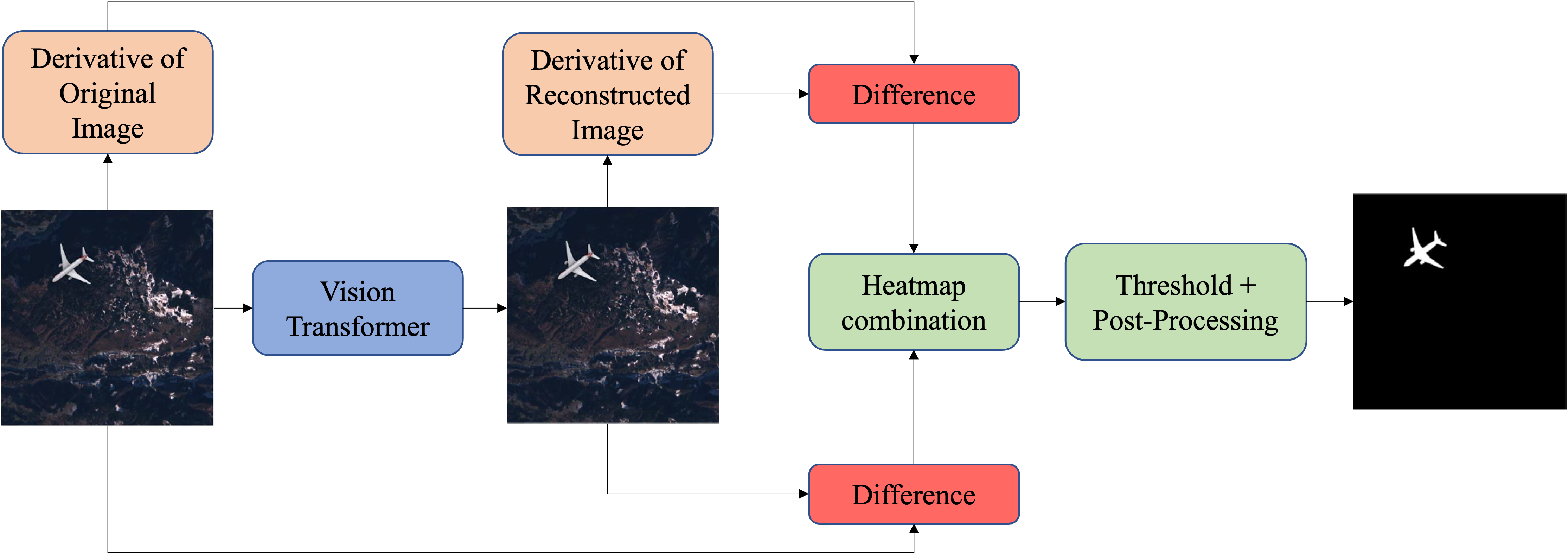
Figure 15: Vision Transformer pipeline proposed in horvath2021_visiontransformer4detection .

6.3.2 Panchromatic

Panchromatic imagery is a valuable asset for a variety of remote sensing applications. It combines the spectral information of the RGB bands, and as such it appears as a grayscale format of images. Its main feature consists in the broader wavelength range it represents. This translates in a greater spatial resolutions. For this reason, a common use for this modality of data is pan-sharpening, i.e., the combination with RGB and multi-spectral data to increase the resolution of the latter.

Due to their importance, in cannas2022panchromatic Cannas et al. investigate the problem of splicing localization for panchromatic data. This work builds upon the concept of image source attribution, which is a task widely studied in the forensic literature for natural images Kirchner2015forensic . More specifically, cannas2021open shows that it is possible to understand which satellite has been used to generate a panchromatic image by means of a carefully trained ensemble of CNNs.

Building upon cannas2021open , cannas2022panchromatic exploits CNNs to spot copy-paste attacks, i.e., splicing attacks where the the spliced region $\mathcal{S}$ comes from a sample captured by a different sensor. The main idea is that it is possible to extract local traces that link an image region to the satellite used for its acquisition. If traces of multiple satellites are found, then the image contains a spliced region.

To implement this idea, the authors first train an ensemble of N different CNNs to perform sensor attribution on pristine images, i.e., assign an input $\mathbf{X}_{\text{Pan}}$ to one of $M$ available satellites in a patch-by-patch fashion. They exploit the same data collection procedure followed in cannas2021open , training each network in the ensemble on a different subset of satellites in order to make the ensemble more robust to changes in data distributions.

At test time, the $n$-th CNN of the ensemble extracts from each patch $\mathbf{P}^{i}$ a feature vector

$$\mathbf{f}^{i}_{n}=[f_{n}^{1},\;f_{n}^{2},\;\dots,\;f_{n}^{M}],$$ (13)

where the $m$-th element is the likelihood for that patch to belong to the $m$-th satellite.

To spot copy-paste attacks, the authors propose to capture the deviation of sensor feature vectors extracted from each image patch with respect to the average sensor feature vector characterizing the image. Deviations from this global descriptor likely indicate that one of the vectors (i.e., one of the patches) comes from a satellite that is different from the one that captured the rest of the image, indicating a copy-paste attack.

Formally, this is done for each CNN by computing the average sensor feature of the image under analysis as the arithmetic mean of all $\mathbf{f}^{i}_{n}$ vectors over $i$ (i.e., over all patches). The deviation is computed as the L2 distance between the average feature and each vector $\mathbf{f}^{i}_{n},\,\forall i$. By assigning to each patch the deviation from the average feature, the authors build a tampering mask $\tilde{\mathbf{M}}_{n}$. Repeating the procedure for all networks in the ensemble, Cannas et al. generate different estimate tampering masks, which are aggregated into an estimate tampering mask $\tilde{\mathbf{M}}$ through a weighted averaging procedure. Figure 16 presents a graphical representation summarizing the whole pipeline.

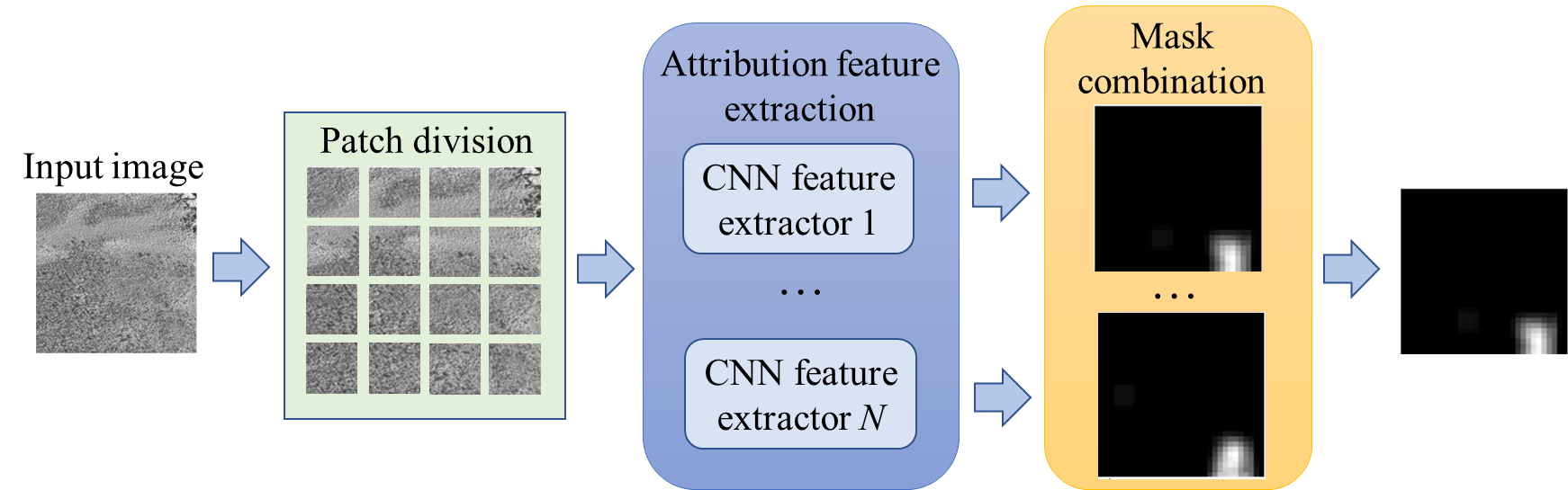
Figure 16: Panchromatic copy-paste localization pipeline proposed in cannas2022panchromatic .

6.3.3 SAR images

Even if SAR images are complex radar signals, amplitude-based products gained a lot of popularity recently. This is also thanks to the many platforms, such as the Copernicus Open Acces Hub, which offer them in easy to manage formats. Unfortunately, such products (e.g., those of the Sentinel-1 mission) are also easy to manipulate as they can be edited by relying on any common image processing suite (e.g., Photoshop).

For this reason, in cannas2022amplitude the authors analyze the problem of splicing localization in amplitude SAR imagery. The basic idea behind their approach is that each SAR product is characterized by peculiar processing traces due to the complex pipeline needed to generate it. Hence, the authors rely on a CNN purposely trained to extract processing traces relative to the overall generation pipeline of amplitude SAR products. These traces are expressed as a fingerprint of the same resolution of the analyzed image, the fingerprint image, which highlights, with different patterns, regions that underwent different processing operations. In this way, spliced regions $\mathcal{S}$ are highlighted as spots with a different texture. Fig.  17 provides an example of a fingerprint computed as in cannas2022amplitude .

After extraction, the fingerprint is analyzed to produce a binary tampering mask $\hat{\mathbf{M}}$ localizing precisely the spliced pixels. The authors experiment with both unsupervised and supervised techniques that turn the fingerprint into a binary mask, testing their solutions on a dataset of spliced samples created starting from GRD images downloaded from the Copernicus Open Access Hub and using different kinds of editing to conceal the spliced area $\mathcal{S}$.

(a) Spliced $\mathbf{X}_{\text{SAR}}$.

(b) Tampering mask $\mathbf{M}_{\text{SAR}}$.

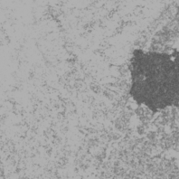
(c) Extracted fingerprint.

Figure 17: Examples of SAR forged image LABEL:sub@fig:sar_spliced, ground truth tampering mask LABEL:sub@fig:sar_gt, and fingerprint LABEL:sub@fig:sar_finger extracted by the method proposed in cannas2022amplitude .

7 Discussion and future challenges

In this section, we recap the possibilities available today to generate and manipulate satellite images, and the techniques investigators and users can adopt to detect non-genuine satellite images, highlighting their main limitations in order to pave the way to future work.

7.1 Synthetic overhead imagery generation

In Section 4, we have overviewed different approaches to create satellite images from scratch or to manipulate their semantic content using generative models. Additionally, in Section 5 we have shown how it is possible to further edit satellite images through techniques that allow to enhance their quality and change their image type. In light of this, it is easy to understand how these techniques could be used by malicious users, allowing them to create high-quality synthetic forgeries of various types. At the same time, generation techniques are far from perfect. All methods developed so far have some limitations that offer new opportunities for future research.

One of the limitation common to all the techniques developed so far is that they do not work on full resolution remote sensing data. They rather consider small image patches up to a resolution of 512$\times$512 pixels. This is due to the inability of the current generative models to store into the memory of GPUs full satellite images, which are usually characterized by resolutions that can reach the gigapixel. This means that a high-resolution synthetic image can only be obtained by stitching together multiple smaller patches. This is sub-optimal from a visual point of view, and leaves traces that can in principle be exploited by forensics detectors.

Another aspect that is often overlooked is related to the fact that some kinds of satellite images have peculiar characteristics that make them very different from natural photographs. These characteristics are not always properly taken into account. For instance, multi-spectral and hyper-spectral data are characterized by correlated multiple bands, whereas most generation techniques usually generate single bands independently. SAR images are complex in nature (i.e., a phase term is also present in addition to the amplitude image) but generation techniques developed so far, focused mainly on the image amplitude. Many kinds of satellite images come with 10 to 16 bit of depths, but generation techniques typically return 8 bit data. All of these aspects should be taken into account by future generators in order to produce realistic satellite images.

Another important characteristic of satellite images is that they are accompanied by abundant metadata. For instance, metadata can provide information related to the kind and position of the satellite used for acquisition, the kind of processing images have undergone to facilitate visual inspection, positional data allowing to geo-locate the image on the planet’s surface, as well as other custom data spanning from land-cover information to digital elevation models providing altitude details. These pieces of information are often completely stripped out by synthetic image generators that only work considering raster images in the pixel domain. On the contrary, it would be advisable to take metadata into account during the generation process in order to further increase the quality and plausibility of the synthetic images. Moreover, it would be interesting to allow generators to be driven by metadata themselves (e.g., to generate an image that is coherent with a set of imposed metadata in terms of geo-location, pixel elevation, land-cover, etc.).

If some of these limitations will be naturally solved in the (near) future thanks to technological improvements (e.g., GPU memory cost will decrease allowing to generate higher resolution data), others pose research challenges that require the development of new ad-hoc methods.

7.2 Forensic analysis of satellite images

Section  6 illustrated how the multimedia forensics community has started paying attention to overhead imagery. Despite the few works published so far, researchers have recognized the strategic role of this kind of data. Therefore a significant growth in the number of contributions is expected in the near future.

One aspect that is stressed in several works is that the nature of satellite images may strongly differ from that of natural photographs. This is evident for SAR data and MSI, but it also holds for EO products, whose complex processing pipelines have little in common with the life cycle of standard digital pictures. This drives the need for specific forensic tools tailored to overhead data.

These tools nowadays often rely on deep learning techniques. This is possible thanks to the increasing availability of EO products on the Web. As a consequence, many of the proposed forensic tools ended up relying on data-driven technology, causing two possible issues. On one hand, common CNN techniques developed for image analysis are tailored to work with 8 bit images with standard photograph resolutions. These tools have to be adapted to work with 16 bit data at higher resolution, which may cause both numerical instability and memory issues. On the other hand GAN-based methods often look like black boxes that offer little to no interpretation to analysts. This is a major concern as forensic results must be supported by strong evidence in courts of trials. Therefore, we foresee as a future research line the development and implementation of explainable forensic tools, which allow a forensic analyst to better understand why a certain decision has been taken.

Another relevant aspect that current detectors have not exploited yet is the presence of multiple image modalities. Satellite images often come bundled with additional images. For instance, it is customary to work with multiple bands if we think at MSIs. Moreover, it is common to have pairs of SAR and EO observations of the same region. This could be exploited by forensic detectors to further verify image integrity by means of a joint analysis of different modalities.

Similarly, we expect that metadata could become an additional asset in the hands of forensic analysts. Indeed, as satellite images often come with a great amount of additional side information, this could be exploited to verify if an image is authentic or it has been modified. This aspect could be of paramount importance not only for methods linking images to devices, but also for local forgery analysis (e.g., verify the compatibility of shadows with the sun position and acquisition time).

Finally, we believe that model-based solutions could still be viable techniques in the detection of satellite image forgeries. As this kind of images undergo a set of very specific operations at acquisition time (e.g., multiple acquisition stitching, image projection from the earth surface to a planar bi-dimensional image, multiple band fusion, etc.) an informed analyst could spot interesting forensic traces that may be not visible upon visual inspection. Detectors based on such traces may only come from a close collaboration between the multimedia forensic community and the remote sensing one.

8 Conclusion

We have reviewed the different facets characterizing the generation of synthetic satellite images. In our analysis, we have divided SOTA works depending on the envisaged application. In doing so, we have seen that several techniques enable image generation from scratch, while others aim at satellite modality translation and image quality improvement. The vast majority of these techniques has been developed to support a wide range of remote sensing applications. Indeed, due to the diffusion of deep learning tools also in the satellite field, the need for precise and annotated data has become more pressing than before. Despite the numerous sources of remote sensing data available on the Web freesat , the use of synthetically generated images can be of great help.

On the negative side, the malicious use of synthetically generated satellite images can lead to severe consequences. As a matter of fact, the increased availability of remote sensing data, while paving the way to numerous research and application opportunities, also exposes this kind of information to manipulations and attacks russia . For this reason, we have also overviewed the forensic tools available to contrast the inappropriate usage of synthetic satellite images. From this analysis, it is evident that satellite imagery represents a complete new challenge to forensic analysts. In particular, detection and localization of synthetic forgeries have been seldom studied in the literature so far. Luckily, different general-purpose forgery detection and localization methods tailored to both EO and SAR imagery have been proposed in the recent literature. We envision that these techniques can be adapted to the problem of exposing synthetic manipulations too.

We are confident that our work will help shedding light on the opportunities that are opening in the near future, as well as on the challenges practitioners must face with regarding the generation and the analysis of synthetic satellite images. In particular, while data generation techniques seem to have reached quite an advanced status, forensic analysis of this kind of imagery still falls behind. As the forensic research community is still making its first steps in the remote sensing field area, the increasing role that satellite images are acquiring in an ever growing number of applications shows the urgent need for the development of appropriate forensic tools.

In this context, future work could be dedicated to the extraction of forensics footprints characterizing the life-cycle of satellite imagery, or to the development of methods that take into account the physical properties of the depicted scene (i.e., physical interpretable methods). Moreover, since many forensics methods are currently based on deep learning tools, other research lines may touch the field of artificial intelligence interpretability and the fusion of traces extracted from different forensics methods.

References

- (1) V. Lappas and V. Kostopoulos, “A survey on small satellite technologies and space missions for geodetic applications,” in Satellites Missions and Technologies for Geosciences, V. Demyanov and J. Becedas, Eds. Rijeka: IntechOpen, 2020, ch. 8. [Online]. Available: https://doi.org/10.5772/intechopen.92625
- (2) P. R. Purnamasayangsukasih, K. Norizah, A. A. M. Ismail, and I. Shamsudin, “A review of uses of satellite imagery in monitoring mangrove forests,” IOP Conference Series: Earth and Environmental Science, vol. 37, p. 012034, jun 2016. [Online]. Available: https://doi.org/10.1088/1755-1315/37/1/012034
- (3) CNN, New satellite images show buildup of Russian military around Ukraine, March 2022 (accessed March 11, 2022), https://edition.cnn.com/2022/02/02/europe/russia-troops-ukraine-buildup-satellite-images-intl/index.html.
- (4) T. Guardian, Mariupol bombing: before and after satellite images show destruction in Ukraine city, March 2022 (accessed March 11, 2022), https://www.theguardian.com/world/2022/mar/10/mariupol-bombing-ukraine-before-and-after-satellite-images-map-russian-attack-residential-maternity-childrens-hospital.
- (5) Mashable, Satellite images show clearly that Russia faked its MH17 report, May 2015 (accessed March 11, 2022), http://mashable.com/2015/05/31/russia-fake-mh17-report.
- (6) G. Rannard, Australia fires: Misleading maps and pictures go viral, January 2020 (accessed June, 2022), https://www.bbc.com/news/blogs-trending-51020564.
- (7) J. Wakefield, Ukraine crisis: Satellite data firm asks for war images, January 2020 (accessed June, 2022).
- (8) P. Isola, J. Zhu, T. Zhou, and A. A. Efros, “Image-to-image translation with conditional adversarial networks,” in 2017 IEEE Conference on Computer Vision and Pattern Recognition, CVPR 2017, Honolulu, HI, USA, July 21-26, 2017. IEEE Computer Society, 2017, pp. 5967–5976.
- (9) J. Zhu, T. Park, P. Isola, and A. Efross, “Unpaired image-to-image translation using cycle-consistent adversarial networks,” IEEE International Conference on Computer Vision (ICCV), 2017.
- (10) A. Piva, “An overview on image forensics,” ISRN Signal Processing, vol. 2013, p. 22, November 2013.
- (11) A. C. Popescu and H. Farid, “Exposing digital forgeries by detecting traces of resampling,” IEEE Transactions on signal processing, vol. 53, no. 2, pp. 758–767, 2005.
- (12) M. Kirchner, “Fast and reliable resampling detection by spectral analysis of fixed linear predictor residue,” in ACM workshop on Multimedia and Security (MM&Sec), 2008.
- (13) T. Bianchi and A. Piva, “Detection of nonaligned double jpeg compression based on integer periodicity maps,” IEEE transactions on Information Forensics and Security, vol. 7, no. 2, pp. 842–848, 2011.
- (14) S. Mandelli, N. Bonettini, P. Bestagini, V. Lipari, and S. Tubaro, “Multiple jpeg compression detection through task-driven non-negative matrix factorization,” in 2018 IEEE International Conference on Acoustics, Speech and Signal Processing (ICASSP). IEEE, 2018, pp. 2106–2110.
- (15) D. Cozzolino, G. Poggi, and L. Verdoliva, “Splicebuster: A new blind image splicing detector,” in IEEE International Workshop on Information Forensics and Security (WIFS), 2015.
- (16) B. Bayar and M. C. Stamm, “A deep learning approach to universal image manipulation detection using a new convolutional layer,” Proceedings of the ACM Workshop on Information Hiding and Multimedia Security, pp. 5–10, June 2016, Vigo, Spain.
- (17) L. Bondi, S. Lameri, D. Güera, P. Bestagini, E. J. Delp, and S. Tubaro, “Tampering detection and localization through clustering of camera-based CNN features,” Proceedings of the IEEE Conference on Computer Vision and Pattern Recognition Workshops, pp. 1855–1864, July 2017, Honolulu, HI. [Online]. Available: dx.doi.org/10.1109/CVPRW.2017.232
- (18) D. Cozzolino and L. Verdoliva, “Noiseprint: a CNN-based camera model fingerprint,” IEEE Transactions on Information Forensics and Security (TIFS), vol. 15, pp. 144–159, 2020.
- (19) N. Bonettini, P. Bestagini, S. Milani, and S. Tubaro, “On the use of Benford’s law to detect GAN-generated images,” in International Conference on Pattern Recognition (ICPR), 2021.
- (20) S. Mandelli, N. Bonettini, P. Bestagini, and S. Tubaro, “Training cnns in presence of jpeg compression: Multimedia forensics vs computer vision,” in IEEE International Workshop on Information Forensics and Security (WIFS), 2020, pp. 1–6.
- (21) O. Alamayreh and M. Barni, “Detection of gan-synthesized street videos,” in European Signal Processing Conference (EUSIPCO), 2021, pp. 811–815.
- (22) D. Gragnaniello, F. Marra, and L. Verdoliva, Detection of AI-Generated Synthetic Faces. Springer International Publishing, 2022, pp. 191–212.
- (23) C. Toth and G. Jóźków, “Remote sensing platforms and sensors: A survey,” ISPRS Journal of Photogrammetry and Remote Sensing, 2016.
- (24) P. University, Optical Sensors overview, November 2020 (accessed November 20, 2020), https://www.e-education.psu.edu/geog480/node/444.
- (25) M. Technologies, Radiometric Use of WorldView-2 Imagery - Technical Note, November 2010 (accessed March 11, 2022).
- (26) P. L. PBC, Planet Imagery Products Specifications, March 2022 (accessed March 13, 2022).
- (27) P. M. Teillet, “Image correction for radiometric effects in remote sensing,” International Journal of Remote Sensing, 1986. [Online]. Available: https://doi.org/10.1080/01431168608948958
- (28) W. Foundation, Orthorectification explanation, November 2020 (accessed November 20, 2020), https://en.wikipedia.org/wiki/Orthophoto.
- (29) J. Harsanyi and C.-I. Chang, “Hyperspectral image classification and dimensionality reduction: an orthogonal subspace projection approach,” IEEE Transactions on Geoscience and Remote Sensing, 1994.
- (30) A. Moreira, P. Prats-Iraola, M. Younis, G. Krieger, I. Hajnsek, and K. P. Papathanassiou, “A tutorial on synthetic aperture radar,” IEEE Geoscience and Remote Sensing Magazine, 2013.
- (31) E. S. Agency, Radar Course 2, June 2021 (accessed June 26, 2021).
- (32) K. Tomiyasu, “Tutorial review of synthetic-aperture radar (sar) with applications to imaging of the ocean surface,” Proceedings of the IEEE, 1978.
- (33) C. Oliver and S. Quegan, Understanding Synthetic Aperture Radar Images, 2004.
- (34) G. Geography, 15 Free Satellite Imagery Data Sources, August 2017 (accessed January 1st, 2022), http://gisgeography.com/free-satellite-imagery-data-list.
- (35) “Aviris,” https://aviris.jpl.nasa.gov/, accessed: February 2022.
- (36) “Copernicus hub,” https://sentinels.copernicus.eu/web/sentinel/user-guides/sentinel-2-msi.
- (37) “Sentinel 1,” https://sentinels.copernicus.eu/web/sentinel/missions/sentinel-1, note = Accessed: February 2022.
- (38) “Sentinel msi,” https://sentinels.copernicus.eu/web/sentinel/user-guides/sentinel-2-msi, accessed: February 2022.
- (39) M. Technologies, Maxar DigitalGlobe Discover Portal, accessed March 14, 2022, https://discover.digitalglobe.com.
- (40) DigitalGlobe, DigitalGlobe Core Imagery Products Guide, November 2010 (accessed March 14, 2022).
- (41) L. mission, U.S. Geological Survey - Landsat Data Access, March 2022 (accessed March 14, 2022), https://www.usgs.gov/landsat-missions/landsat-data-access.
- (42) NASA, Landsat Science, March 2022 (accessed March 14, 2022), https://landsat.gsfc.nasa.gov/.
- (43) M. Schmitt, L. H. Hughes, C. Qiu, and X. X. Zhu, “Sen12ms – a curated dataset of georeferenced multi-spectral sentinel-1/2 imagery for deep learning and data fusion,” in ISPRS Annals of the Photogrammetry, Remote Sensing and Spatial Information Sciences, vol. IV-2/W7, 2019, pp. 153–160.
- (44) NASA, Moderate Resolution Imagery Spectroradiometer (MODIS), June 2022 (accessed June 22, 2022), https://modis.gsfc.nasa.gov/about/.
- (45) I. Goodfellow, J. Pouget-Abadie, M. Mirza, B. Xu, D. Warde-Farley, S. Ozair, A. Courville, and Y. Bengio, “Generative adversarial nets,” in Advances in Neural Information Processing Systems, Z. Ghahramani, M. Welling, C. Cortes, N. Lawrence, and K. Q. Weinberger, Eds., vol. 27. Curran Associates, Inc., 2014.
- (46) L. Yu, W. Zhang, J. Wang, and Y. Yu, “Seqgan: Sequence generative adversarial nets with policy gradient,” in Proceedings of the Thirty-First AAAI Conference on Artificial Intelligence, 2017.
- (47) S. Kazeminia, C. Baur, A. Kuijper, B. van Ginneken, N. Navab, S. Albarqouni, and A. Mukhopadhyay, “Gans for medical image analysis,” Artificial Intelligence in Medicine, 2020.
- (48) T. Karras, T. Aila, S. Laine, and J. Lehtinen, “Progressive growing of gans for improved quality, stability, and variation,” in 6th International Conference on Learning Representations, ICLR 2018, Vancouver, BC, Canada, April 30 - May 3, 2018, Conference Track Proceedings. OpenReview.net, 2018.
- (49) T. Karras, S. Laine, and T. Aila, “A style-based generator architecture for generative adversarial networks,” in IEEE Conference on Computer Vision and Pattern Recognition, CVPR 2019, Long Beach, CA, USA, June 16-20, 2019. Computer Vision Foundation / IEEE, 2019, pp. 4401–4410.
- (50) T. Karras, S. Laine, M. Aittala, J. Hellsten, J. Lehtinen, and T. Aila, “Analyzing and improving the image quality of stylegan,” in 2020 IEEE/CVF Conference on Computer Vision and Pattern Recognition, CVPR 2020, Seattle, WA, USA, June 13-19, 2020. Computer Vision Foundation / IEEE, 2020, pp. 8107–8116.
- (51) M. Mirza and S. Osindero, “Conditional generative adversarial nets,” CoRR, vol. abs/1411.1784, 2014. [Online]. Available: http://arxiv.org/abs/1411.1784
- (52) R. Chen, W. Huang, B. Huang, F. Sun, and B. Fang, “Reusing discriminators for encoding: Towards unsupervised image-to-image translation,” in 2020 IEEE/CVF Conference on Computer Vision and Pattern Recognition, CVPR 2020, Seattle, WA, USA, June 13-19, 2020. Computer Vision Foundation / IEEE, 2020, pp. 8165–8174.
- (53) I. Gulrajani, F. Ahmed, M. Arjovsky, V. Dumoulin, and A. C. Courville, “Improved training of wasserstein gans,” in Advances in Neural Information Processing Systems 30: Annual Conference on Neural Information Processing Systems 2017, December 4-9, 2017, Long Beach, CA, USA, I. Guyon, U. von Luxburg, S. Bengio, H. M. Wallach, R. Fergus, S. V. N. Vishwanathan, and R. Garnett, Eds., 2017, pp. 5767–5777.
- (54) M. Arjovsky, S. Chintala, and L. Bottou, “Wasserstein generative adversarial networks,” in Proceedings of the 34th International Conference on Machine Learning, ICML 2017, Sydney, NSW, Australia, 6-11 August 2017, ser. Proceedings of Machine Learning Research, D. Precup and Y. W. Teh, Eds., vol. 70. PMLR, 2017, pp. 214–223.
- (55) D. P. Kingma and M. Welling, “Auto-encoding variational bayes,” in 2nd International Conference on Learning Representations, ICLR 2014, Banff, AB, Canada, April 14-16, 2014, Conference Track Proceedings, Y. Bengio and Y. LeCun, Eds., 2014. [Online]. Available: http://arxiv.org/abs/1312.6114
- (56) G. E. Hinton and R. Zemel, “Autoencoders, minimum description length and helmholtz free energy,” in Advances in Neural Information Processing Systems (NIPS), 1993.
- (57) J. Guo, B. Lei, C. Ding, and Y. Zhang, “Synthetic aperture radar image synthesis by using generative adversarial nets,” IEEE Geosci. Remote. Sens. Lett., vol. 14, no. 7, pp. 1111–1115, 2017.
- (58) Y. Zhan, D. Hu, Y. Wang, and X. Yu, “Semisupervised hyperspectral image classification based on generative adversarial networks,” IEEE Geoscience and Remote Sensing Letters, vol. 15, no. 2, pp. 212–216, 2018.
- (59) L. Abady, M. Barni, A. Garzelli, and B. Tondi, “GAN generation of synthetic multispectral satellite images,” in Image and Signal Processing for Remote Sensing XXVI, L. Bruzzone, F. Bovolo, and E. Santi, Eds., vol. 11533, International Society for Optics and Photonics. SPIE, 2020, pp. 122 – 133. [Online]. Available: https://doi.org/10.1117/12.2575765
- (60) C. X. Ren, A. Ziemann, J. Theiler, and J. Moore, “Deepfaking it: experiments in generative, adversarial multispectral remote sensing,” in Algorithms, Technologies, and Applications for Multispectral and Hyperspectral Imaging XXVII, 2021.
- (61) B. Zhao, S. Zhang, C. Xu, Y. Sun, and C. Deng, “Deep fake geography? when geospatial data encounter artificial intelligence,” Cartography and Geographic Information Science, vol. 48, no. 4, pp. 338–352, 2021. [Online]. Available: https://doi.org/10.1080/15230406.2021.1910075
- (62) S. Auer, S. Hinz, and R. Bamler, “Ray-tracing simulation techniques for understanding high-resolution sar images,” IEEE Transactions on Geoscience and Remote Sensing, vol. 48, no. 3, pp. 1445–1456, 2010.
- (63) A. Radford, L. Metz, and S. Chintala, “Unsupervised representation learning with deep convolutional generative adversarial networks,” in 4th International Conference on Learning Representations, ICLR 2016, San Juan, Puerto Rico, May 2-4, 2016, Conference Track Proceedings, Y. Bengio and Y. LeCun, Eds., 2016.
- (64) “Qgis,” https://www.qgis.org/, accessed: May 2022.
- (65) W. He and N. Yokoya, “Multi-temporal sentinel-1 and -2 data fusion for optical image simulation,” ISPRS Int. J. Geo Inf., vol. 7, no. 10, p. 389, 2018. [Online]. Available: https://doi.org/10.3390/ijgi7100389
- (66) N. Merkle, S. Auer, R. Müller, and P. Reinartz, “Exploring the potential of conditional adversarial networks for optical and SAR image matching,” IEEE J. Sel. Top. Appl. Earth Obs. Remote. Sens., vol. 11, no. 6, pp. 1811–1820, 2018.
- (67) K. Enomoto, K. Sakurada, W. Wang, N. Kawaguchi, M. Matsuoka, and R. Nakamura, “Image translation between sar and optical imagery with generative adversarial nets,” in IGARSS 2018 - 2018 IEEE International Geoscience and Remote Sensing Symposium, 2018, pp. 1752–1755.
- (68) L. Liu and B. Lei, “Can sar images and optical images transfer with each other?” in IGARSS 2018 - 2018 IEEE International Geoscience and Remote Sensing Symposium, 2018, pp. 7019–7022.
- (69) M. Fuentes Reyes, S. Auer, N. Merkle, C. Henry, and M. Schmitt, “Sar-to-optical image translation based on conditional generative adversarial networks-optimization, opportunities and limits,” Remote Sensing, vol. 11, no. 17, 2019. [Online]. Available: https://www.mdpi.com/2072-4292/11/17/2067
- (70) J. D. Bermudez, P. N. Happ, R. Q. Feitosa, and D. A. Oliveira, “Synthesis of multispectral optical images from sar/optical multitemporal data using conditional generative adversarial networks,” IEEE Geoscience and Remote Sensing Letters, vol. 16, no. 8, pp. 1220–1224, 2019.
- (71) H. J. A. Andrade and B. J. T. Fernandes, “Synthesis of satellite-like urban images from historical maps using conditional gan,” IEEE Geoscience and Remote Sensing Letters, pp. 1–4, 2020.
- (72) X. Yuan, J. Tian, and P. Reinartz, “Generating artificial near infrared spectral band from rgb image using conditional generative adversarial network,” ISPRS Annals of the Photogrammetry, Remote Sensing and Spatial Information Sciences, vol. V-3-2020, pp. 279–285, 2020. [Online]. Available: https://www.isprs-ann-photogramm-remote-sens-spatial-inf-sci.net/V-3-2020/279/2020/
- (73) T. Vandal, D. McDuff, W. Wang, K. Duffy, A. R. Michaelis, and R. R. Nemani, “Spectral synthesis for geostationary satellite-to-satellite translation,” IEEE Trans. Geosci. Remote. Sens., vol. 60, pp. 1–11, 2022.
- (74) M. Schmitt, L. Hughes, M. Körner, and X. X. Zhu, “Colorizing sentinel-1 SAR images using a variational autoencoder conditioned on sentinel-2 imagery,” The International Archives of the Photogrammetry, Remote Sensing and Spatial Information Sciences (ISSN: 1682-1750), vol. 42, pp. 1045–1051, 2018.
- (75) O. Tasar, S. L. Happy, Y. Tarabalka, and P. Alliez, “Colormapgan: Unsupervised domain adaptation for semantic segmentation using color mapping generative adversarial networks,” IEEE Trans. Geosci. Remote. Sens., vol. 58, no. 10, pp. 7178–7193, 2020.
- (76) K. Enomoto, K. Sakurada, W. Wang, H. Fukui, M. Matsuoka, R. Nakamura, and N. Kawaguchi, “Filmy cloud removal on satellite imagery with multispectral conditional generative adversarial nets,” in Proceedings of the IEEE Conference on Computer Vision and Pattern Recognition Workshops, 2017, pp. 48–56.
- (77) P. Singh and N. Komodakis, “Cloud-gan: Cloud removal for sentinel-2 imagery using a cyclic consistent generative adversarial networks,” in IGARSS 2018 - 2018 IEEE International Geoscience and Remote Sensing Symposium, 2018, pp. 1772–1775.
- (78) C. Grohnfeldt, M. Schmitt, and X. Zhu, “A conditional generative adversarial network to fuse sar and multispectral optical data for cloud removal from sentinel-2 images,” in IGARSS 2018-2018 IEEE International Geoscience and Remote Sensing Symposium. IEEE, 2018, pp. 1726–1729.
- (79) M. Zotov and J. Gamper, “Conditional denoising of remote sensing imagery using cycle-consistent deep generative models,” CoRR, vol. abs/1910.14567, 2019.
- (80) P. Ebel, M. Schmitt, and X. X. Zhu, “Cloud removal in unpaired sentinel-2 imagery using cycle-consistent gan and sar-optical data fusion,” in IGARSS 2020 - 2020 IEEE International Geoscience and Remote Sensing Symposium, 2020, pp. 2065–2068.
- (81) J. Gao, Q. Yuan, J. Li, H. Zhang, and X. Su, “Cloud removal with fusion of high resolution optical and sar images using generative adversarial networks,” Remote Sensing, vol. 12, no. 1, p. 191, 2020.
- (82) V. Sarukkai, A. Jain, B. Uzkent, and S. Ermon, “Cloud removal from satellite images using spatiotemporal generator networks,” in Proceedings of the IEEE/CVF Winter Conference on Applications of Computer Vision, 2020, pp. 1796–1805.
- (83) X. Wen, Z. Pan, Y. Hu, and J. Liu, “Generative adversarial learning in yuv color space for thin cloud removal on satellite imagery,” Remote Sensing, vol. 13, no. 6, 2021. [Online]. Available: https://www.mdpi.com/2072-4292/13/6/1079
- (84) K. He, X. Zhang, S. Ren, and J. Sun, “Deep residual learning for image recognition,” in IEEE Conference on Computer Vision and Pattern Recognition (CVPR), 2016.
- (85) X. Mao, Q. Li, H. Xie, R. Y. K. Lau, Z. Wang, and S. P. Smolley, “Least squares generative adversarial networks,” in IEEE International Conference on Computer Vision, ICCV 2017, Venice, Italy, October 22-29, 2017. IEEE Computer Society, 2017, pp. 2813–2821.
- (86) G. Baier, A. Deschemps, M. Schmitt, and N. Yokoya, “Synthesizing optical and sar imagery from land cover maps and auxiliary raster data,” IEEE Transactions on Geoscience and Remote Sensing, vol. 60, pp. 1–12, 2022.
- (87) T. Park, M. Liu, T. Wang, and J. Zhu, “Semantic image synthesis with spatially-adaptive normalization,” in IEEE Conference on Computer Vision and Pattern Recognition, CVPR 2019, Long Beach, CA, USA, June 16-20, 2019. Computer Vision Foundation / IEEE, 2019, pp. 2337–2346.
- (88) G. Baier, A. Deschemps, M. Schmitt, and N. Yokoya, “Geonrw,” 2020. [Online]. Available: https://dx.doi.org/10.21227/s5xq-b822
- (89) M. S. L. H. P. G. N. Y. R. Hansch, “2020 ieee grss data fusion contest,” 2019. [Online]. Available: https://dx.doi.org/10.21227/rha7-m332
- (90) P. L. Guth, A. V. Niekerk, C. H. Grohmann, J. Muller, L. Hawker, I. V. Florinsky, D. Gesch, H. I. Reuter, V. Herrera-Cruz, S. Riazanoff, C. López-Vázquez, C. C. Carabajal, C. Albinet, and P. Strobl, “Digital elevation models: Terminology and definitions,” Remote. Sens., vol. 13, no. 18, p. 3581, 2021.
- (91) M. Liu, T. M. Breuel, and J. Kautz, “Unsupervised image-to-image translation networks,” in Advances in Neural Information Processing Systems 30: Annual Conference on Neural Information Processing Systems 2017, December 4-9, 2017,Long Beach, CA, USA, I. Guyon, U. von Luxburg, S. Bengio, H. M. Wallach, R. Fergus, S. V. N. Vishwanathan, and R. Garnett, Eds., 2017, pp. 700–708.
- (92) A. B. L. Larsen, S. K. Sønderby, H. Larochelle, and O. Winther, “Autoencoding beyond pixels using a learned similarity metric,” in Proceedings of the 33nd International Conference on Machine Learning, ICML 2016, New York City, NY, USA, June 19-24, 2016, ser. JMLR Workshop and Conference Proceedings, M. Balcan and K. Q. Weinberger, Eds., vol. 48. JMLR.org, 2016, pp. 1558–1566.
- (93) M. Liu, T. M. Breuel, and J. Kautz, “Unsupervised image-to-image translation networks,” in Advances in Neural Information Processing Systems 30: Annual Conference on Neural Information Processing Systems 2017, December 4-9, 2017, Long Beach, CA, USA, I. Guyon, U. von Luxburg, S. Bengio, H. M. Wallach, R. Fergus, S. V. N. Vishwanathan, and R. Garnett, Eds., 2017, pp. 700–708.
- (94) A. Deshpande, J. Lu, M. Yeh, M. J. Chong, and D. A. Forsyth, “Learning diverse image colorization,” in 2017 IEEE Conference on Computer Vision and Pattern Recognition, CVPR 2017, Honolulu, HI, USA, July 21-26, 2017. IEEE Computer Society, 2017, pp. 2877–2885.
- (95) C. M. Bishop, “Mixture density networks,” Tech. Rep., 1994.
- (96) H. Pauli, “Cie recommendations on uniform color spaces, color-difference equations, and metric color terms,” Color Research & Application, vol. 2, no. 1, pp. 5–6, 1977.
- (97) K. Perlin, “Improving noise,” ACM Trans. Graph., vol. 21, no. 3, p. 681–682, jul 2002.
- (98) X. Wang, G. Xu, Y. Wang, D. Lin, P. Li, and X. Lin, “Thin and thick cloud removal on remote sensing image by conditional generative adversarial network,” in IGARSS 2019 - 2019 IEEE International Geoscience and Remote Sensing Symposium, 2019, pp. 1426–1429.
- (99) P. Tucker, The Newest AI-Enabled Weapon: ‘Deep-Faking’ Photos of the Earth, 31 March 2019 (accessed August 8, 2022), https://www.defenseone.com/technology/2019/03/next-phase-ai-deep-faking-whole-world-and-china-ahead/155944/.
- (100) T. Fawcett, “An introduction to ROC analysis,” Pattern Recognit. Lett., vol. 27, no. 8, pp. 861–874, 2006.
- (101) A. A. Taha and A. Hanbury, “Metrics for evaluating 3d medical image segmentation: analysis, selection, and tool,” BMC Medical Imaging, vol. 15, p. 29, 2015.
- (102) H. He and Y. Ma, Imbalanced Learning: Foundations, Algorithms, and Applications, 1st ed. Wiley-IEEE Press, 2013.
- (103) C. D. Manning and H. Schütze, Foundations of statistical natural language processing. MIT Press, 2001.
- (104) S. Yarlagadda, D. Güera, P. Bestagini, F. Zhu, S. Tubaro, and E. Delp, “Satellite image forgery detection and localization using GAN and one-class classifier,” in Electronic Imaging (EI), 2018.
- (105) E. R. Bartusiak, S. K. Yarlagadda, D. Güera, P. Bestagini, S. Tubaro, F. M. Zhu, and E. J. Delp, “Splicing detection and localization in satellite imagery using conditional GANs,” in IEEE Conference on Multimedia Information Processing and Retrieval (MIPR), 2019.
- (106) J. Horvàth, D. Güera, S. K. Yarlagadda, P. Bestagini, F. M. Zhu, S. Tubaro, and E. J. Delp, “Anomaly-based manipulation detection in satellite images,” in IEEE Conference on Computer Vision and Pattern Recognition Workshop (CVPRW), 2019.
- (107) D. Mas Montserrat, J. Horvàth, S. K. Yarlagadda, F. M. Zhu, and E. J. Delp, “Generative autoregressive ensembles for satellite imagery manipulation detection,” in IEEE International Workshop on Information Forensics and Security (WIFS), 2020.
- (108) J. Horvàth, D. Mas Montserrat, H. Hao, and E. J. Delp, “Manipulation detection in satellite images using deep belief networks,” in IEEE Conference on Computer Vision and Pattern Recognition Workshop (CVPRW), 2020.
- (109) J. Horváth, S. Baireddy, H. Hao, D. M. Montserrat, and E. J. Delp, “Manipulation detection in satellite images using vision transformer,” in 2021 IEEE/CVF Conference on Computer Vision and Pattern Recognition Workshops (CVPRW), 2021, pp. 1032–1041.
- (110) J. Horváth, D. M. Montserrat, E. J. Delp, and J. Horváth, “Nested attention u-net: A splicing detection method for satellite images,” in Pattern Recognition. ICPR International Workshops and Challenges, A. Del Bimbo, R. Cucchiara, S. Sclaroff, G. M. Farinella, T. Mei, M. Bertini, H. J. Escalante, and R. Vezzani, Eds. Cham: Springer International Publishing, 2021, pp. 516–529.
- (111) H. Chen, K. Zhang, S. Hu, S. You, and C. J. Kuo, “Geo-defakehop: High-performance geographic fake image detection,” CoRR, vol. abs/2110.09795, 2021. [Online]. Available: https://arxiv.org/abs/2110.09795
- (112) E. D. Cannas, N. Bonettini, S. Mandelli, P. Bestagini, and S. Tubaro, “Amplitude SAR imagery splicing localization,” IEEE Access, 2022.
- (113) E. D. Cannas, J. Horváth, S. Baireddy, P. Bestagini, E. J. Delp, and S. Tubaro, “Panchromatic imagery copy-paste localization through data-driven sensor attribution,” in IEEE International Conference on Acoustics, Speech and Signal Processing (ICASSP), 2022.
- (114) T. Chen and C. Guestrin, “Xgboost: A scalable tree boosting system,” in Proceedings of the 22nd ACM SIGKDD International Conference on Knowledge Discovery and Data Mining, 2016.
- (115) M. Sundararajan, A. Taly, and Q. Yan, “Axiomatic attribution for deep networks,” in Proceedings of the International Conference on Machine Learning, 2017.
- (116) L. Verdoliva, “Deep learning in multimedia forensics,” in Proceedings of the 6th ACM Workshop on Information Hiding and Multimedia Security, 2018.
- (117) L. Ruff, R. A. Vandermeulen, N. Görnitz, L. Deecke, S. A. Siddiqui, A. Binder, E. Müller, and M. Kloft, “Deep one-class classification,” in Proceedings of the 35th International Conference on Machine Learning, vol. 80, 2018, pp. 4393–4402.
- (118) G. E. Hinton and R. R. Salakhutdinov, “Reducing the dimensionality of data with neural networks,” Science, 2006.
- (119) D. H. Ackley, G. E. Hinton, and T. J. Sejnowski, “A learning algorithm for boltzmann machines,” Cognitive Science, 1985.
- (120) A. V. Oord, N. Kalchbrenner, and K. Kavukcuoglu, “Pixel recurrent neural networks,” in Proceedings of The 33rd International Conference on Machine Learning, 2016.
- (121) A. van den Oord, N. Kalchbrenner, L. Espeholt, k. kavukcuoglu, O. Vinyals, and A. Graves, “Conditional image generation with pixelcnn decoders,” in Advances in Neural Information Processing Systems, 2016.
- (122) A. Kolesnikov, A. Dosovitskiy, D. Weissenborn, G. Heigold, J. Uszkoreit, L. Beyer, M. Minderer, M. Dehghani, N. Houlsby, S. Gelly, T. Unterthiner, and X. Zhai, “An image is worth 16x16 words: Transformers for image recognition at scale,” 2021.
- (123) M. Kirchner and T. Gloe, “Forensic Camera Model Identification,” in Handbook of Digital Forensics of Multimedia Data and Devices. Chichester, UK: John Wiley & Sons, Ltd, 2015, pp. 329–374.
- (124) E. D. Cannas, S. Baireddy, E. R. Bartusiak, S. K. Yarlagadda, D. Mas Montserrat, P. Bestagini, S. Tubaro, and E. J. Delp, “Open-set source attribution for panchromatic satellite imagery,” in IEEE International Conference on Image Processing (ICIP), 2021.