Asymptotic Normality for the Fourier spot volatility estimator
in the presence of microstructure noise

Abstract

The main contribution of the paper is proving that the Fourier spot volatility estimator introduced in [Malliavin and Mancino, 2002] is consistent and asymptotically efficient if the price process is contaminated by microstructure noise. Specifically, in the presence of additive microstructure noise we prove a Central Limit Theorem with the optimal rate of convergence $n^{1/8}$. The result is obtained without the need for any manipulation of the original data or bias correction. Moreover, we complete the asymptotic theory for the Fourier spot volatility estimator in the absence of noise, originally presented in [Mancino and Recchioni, 2015], by deriving a Central Limit Theorem with the optimal convergence rate $n^{1/4}$. Finally, we propose a novel feasible adaptive method for the optimal selection of the parameters involved in the implementation of the Fourier spot volatility estimator with noisy high-frequency data and provide support to its accuracy both numerically and empirically.

JEL Codes: C02, C13, C14, C58.

Keywords: non-parametric spot volatility estimator, central limit theorem, Fourier analysis, microstructure noise.

1 Introduction

Even though the estimation of the time-varying volatility of financial assets has long been recognized as a relevant topic in financial econometrics (see, e.g., [Andersen et al., 2005] and references therein), in the last couple of decades the increasing availability of high-frequency market data has given an enormous impulse to the investigation of novel estimation methodologies and the exploration of their applications. We refer to [Aït-Sahalia and Jacod, 2014] for an extensive review of the relevant literature. However, unlike the case of the integrated volatility, the non-parametric estimation of the instantaneous (or spot) volatility represents a relatively recent topic. In this paper we study the asymptotic normality of the non-parametric high-frequency estimator of the instantaneous volatility proposed by [Malliavin and Mancino, 2002].

The benchmark for computing the volatility of an asset on a fixed time interval with high-frequency data is provided by the sum of the squared intraday returns (i.e., the realized volatility). In the limit as the time between two consecutive observations converges to zero, the realized volatility converges to the quadratic variation of the asset price process, and its derivative provides the instantaneous volatility thereof. However, the approximation of the derivative of the quadratic variation required to obtain the spot volatility may generate appreciable numerical instabilities. Moreover, high-frequency data are affected by the presence of microstructure effects, which cause a discrepancy between asset pricing theory based on semi-martingales and the actual data sampled at very fine intervals.

Kernel smoothing procedures have been extensively adopted to address numerical instabilities and obtain efficient estimators of the spot volatility. Moreover, modifications of the estimators have been proposed to correct for the bias introduced by the presence of microstructure noise. Such modifications, which rely on the pre-processing of price observations, include the Two-Scale Sub-Sampling method by [Zu and Boswijk, 2014] and the Pre-Averaging method for kernel-based estimators by [Aït-Sahalia and Jacod, 2014] and [Figueroa and Wu, 2022].

This paper deals with an alternative estimation approach, introduced in [Malliavin and Mancino, 2002], which is based on the Fourier series decomposition of the volatility process. The Fourier method reconstructs the instantaneous volatility as a series expansion, with coefficients gathered from the Fourier coefficients of the price variation. Even though the Fourier estimator was originally designed as a global estimator (see also [Malliavin and Mancino, 2009]), it also works well as a point-wise estimator inside the estimation interval. The main contribution of this paper is to provide a complete study of the point-wise asymptotic normality of the Fourier spot volatility estimator, proving that the latter reaches the optimal rate of convergence and variance in the absence and in the presence of additive microstructure noise. This result is achieved without any manipulation of the original data or any bias correction, thus supporting the results obtained in a finite-sample setting by [Mancino and Recchioni, 2015].

Several papers have studied the efficiency of the Fourier method in reconstructing integrated volatility and co-volatilities values, even in the presence of microstructure noise, with a focus on the finite-sample performance, see, e.g., [Barucci and Renò, 2002, Hansen and Lunde, 2006, Nielsen and Frederiksen, 2006, Mancino and Sanfelici, 2008, Mancino and Sanfelici, 2011]. The Central Limit Theorem for the Fourier estimator of the integrated covariance was obtained in [Malliavin and Mancino, 2009], with a sub-optimal rate of convergence, while [Clement and Gloter, 2011] proved the asymptotic normality with the optimal rate and variance under the assumption of irregular and non-synchronous observations.

The point-wise Central Limit Theorem for the Fourier spot volatility estimator in the absence of noise is proved in [Mancino and Recchioni, 2015], with a slightly sub-optimal rate of convergence. Moreover, the authors provide an extensive simulation study showing the accuracy of the resulting spot volatility estimates and their robustness in the presence of different microstructure noise specifications. A modification of the classical Fourier method is proposed in [Cuchiero and Teichmann, 2015] to obtain a jump-robust estimator of the instantaneous covariance, which is not consistent in the presence of microstructure noise. The contribution of various order autocovariances has early been considered by [Zhou, 1996] and then by [Barndorff-Nielsen et al., 2008]. In this spirit, the Fourier spot volatility estimator can be related to a local version of the infinite-lag realized kernels, see [Barndorff-Nielsen et al., 2008]. A different but related study is present in [Park et al., 2016]. In this study, the authors prove the consistency and asymptotic normality for a class of Fourier-type estimators of the Fourier coefficients of the covariance (thus integrated quantities), named Fourier Realized Kernels. The Central Limit theorem for any Fourier coefficient holds under some general conditions that allow for microstructure noise effects and asynchronicity between different assets. The rate of convergence depends on the relative liquidity between assets and reaches the value $n^{1/5}$ if the assets are synchronous. However, the rate of convergence of the spot Fourier Realized Kernel estimator is not investigated. Finally, a Fourier-type spot volatility estimator is considered also in [Mancini et al., 2015]. Nonetheless, the estimator studied in [Mancini et al., 2015], Proposition 4.2, substantially differs from the Fourier spot volatility estimator, precisely being a Féjèr kernel-based realized estimator. In fact, the authors get rid of the cross products, which are the main by-product of the original convolution formula (see [Malliavin and Mancino, 2009]), thus loosing the robustness of the Fourier estimator with respect to microstructure noise.

In this paper, we first fine-tune the result of [Mancino and Recchioni, 2015], that is, under the assumption that the variance process is also a continuous Itô semimartingale, we prove that the Fourier spot volatility estimator attains the optimal rate of convergence, $n^{1/4}$. Secondly, we prove that, in the presence of additive microstructure noise, the rate of convergence attained by the Fourier estimator is optimal, that is, $n^{1/8}$. This is the convergence rate of the spot volatility estimators in [Aït-Sahalia and Jacod, 2014, Section 8.7] and [Figueroa and Wu, 2022, Theorem 2.2], while the Two-Scale realized spot variance in [Zu and Boswijk, 2014, Theorem 2] attains the convergence rate $n^{1/12}$. However, while all these estimators require a preliminary manipulation of price observations and a bias-correction, the Fourier estimator does not need any modification to be robust to microstructure noise. In fact, the efficient implementation of the Fourier spot volatility estimator requires the balancing of three frequencies: the number of log-return observations $n$; the cutting frequency in the convolution formula that yields the Fourier coefficients of the volatility; the number of Fourier coefficients of the volatility to be used in the Fourier inversion formula (respectively, $N$ and $M$ throughout the paper). In the presence of noise, the effect of the latter is ignored by cutting out the highest frequencies in the construction of the Fourier coefficients of the volatility, thereby leading to a noise-robust estimator of the instantaneous volatility. Specifically, while in the absence of noise (see Theorem 3.1) the rate-variance optimal choice of the cutting frequency $N$ is the Nyquist frequency $n/2$, in the presence of noise (see Theorem 4.1) it is optimal to select a smaller $N$, compared to the no-noise case, namely $N=O(n^{1/2})$. The frequency $M$ is optimized as $M=O(N^{1/2})$ in both the absence and the presence of noise.

In this paper, we also conduct a simulation study on the finite-sample performance of the Fourier instantaneous volatility estimator with high-frequency noisy data and provide a refinement of the numerical results presented in [Mancino and Recchioni, 2015] by using as guidance the newly derived asymptotic theory. Specifically, the aim of the simulation study is three-fold.

First, we investigate the relationship between the efficient selection of the parameters $N$ and $M$ and the intensity of the noise. The rate-optimal Central Limit Theorem (see Theorem 4.1) assumes that $N\sim cn^{1/2},\,c>0,$ and $M\sim aN^{1/2},\,a>0,$ as $n,N,M\to\infty$. Thus, the selection of $N$ and $M$ may reduce to choosing the values of the constants $c$ and $a$. For what concerns $c$, simulations suggest that it should be carefully decreased in correspondence of the increase of the noise intensity to preserve the accuracy of the estimator. As for $a$, numerical evidence instead suggests that its optimal value is rather insensitive to the noise level. These findings provide a more robust insight into the sensitivity of the efficiency of the Fourier estimator compared to the numerical study in [Mancino and Recchioni, 2015], where the authors assumed $N\sim(1/2)n^{\alpha}$ and $M\sim(1/16\pi)n^{\beta}$ and attempted to optimize the rates $(\alpha,\beta)$ numerically, in correspondence of different noise intensities and specifications.

Secondly, we introduce a novel feasible adaptive method to select the parameters $N$ and $M$ from market data and evaluate its efficiency numerically. The method is based on the gradient-descent algorithm and optimizes the mean integrated squared error. Under the assumptions that ensure asymptotic normality of the estimation error, the mean integrated squared error can be approximated by the integrated asymptotic error variance at high-frequencies (see [Zu and Boswijk, 2014, Section 3.4]). So far, to the best of our knowledge, the only feasible method available in the literature for selecting $N$ and $M$ was the indirect inference procedure described in [Mancino and Recchioni, 2015, Section 4.2], based on the testing of the empirical distribution of the log-returns standardized by volatility estimates. The integrated asymptotic error variance of the Fourier estimator in the rate-efficient case depends on the integrals of the variance, quarticity and volatility of volatility processes, along with the variance of the noise (see Theorem 4.1). The aforementioned integrated quantities can be estimated by means of non-parametric Fourier estimators (see, resp., [Mancino and Sanfelici, 2008], [Mancino and Sanfelici, 2012] and [Sanfelici et al., 2015]), while the noise variance can be estimated using the estimator proposed by [Bandi and Russell, 2006]. Simulations show that the adaptive method introduced in this paper yields a very satisfactory performance. Moreover, its accuracy is supported also by an empirical exercise, conducted with high-frequency prices of the S&P500 index sampled over the period March, 2018 - April, 2018.

Finally, we compare the performance of the Fourier estimator with that of alternative noise-robust spot volatility estimators. In particular, the comparison conducted in this paper extends the one presented in [Mancino and Recchioni, 2015] by taking into account the recently proposed Pre-averaging kernel estimator by [Figueroa and Wu, 2022]. Numerical results suggest that the Fourier estimator may have a competitive edge w.r.t. the alternative noise-robust estimators, in line with [Mancino and Recchioni, 2015]. However, it is worth underlining that the performance gap w.r.t. the Pre-averaging kernel estimator is smaller in scenarios characterized by higher noise. The findings of the comparative study conducted in this paper are coherent with those of the simulation study by [Mariotti et al., 2022], where the data-generating process is the limit order book simulator by [Huang et al., 2015], which is able to reproduce several microstructural characteristics of financial markets.

The paper is organized as follows. Section 2 contains definitions and assumptions. Asymptotic results in the absence and the presence of microstructure noise are detailed, resp., in Sections 3 and 4. Sections 5 illustrates the simulation study and Section 6 contains the empirical exercise. Section 7 concludes. Appendix A contains the proofs, while Appendix B resumes some auxiliary results on the Féjèr and Dirichlet kernels.

2 Fourier estimator of spot volatility

In this section we introduce the setting and recall the definition of the Fourier estimator of the spot volatility originally proposed in [Malliavin and Mancino, 2002]. The Fourier estimation method consists in a two-step procedure: first the Fourier coefficients of the volatility process are estimated and secondly the volatility path is reconstructed using the Fourier-Féjèr inversion formula.

The following assumptions are made.

(A.I) The price process $p$ is a continuous Itô semimartingale satisfying the stochastic differential equation

$$dp(t)=\sigma(t)\,dW_{t}+b(t)\,dt,$$

where $W$ is a standard Brownian motion on a filtered probability space $(\Omega,({\cal F}_{t})_{t\in[0,T]},P)$ satisfying the usual conditions.

(A.II) The spot volatility process $\sigma^{2}$ is an Itô semimartingale

$$d\sigma^{2}(t)=\gamma(t)dZ_{t}+b_{v}(t)dt,$$

where $Z$ is a standard Brownian motion adapted to the filtration ${\cal F}$ and such that $d\langle W,Z\rangle_{t}=\rho\,dt$, with constant $\rho$.

(A.III) The processes $\sigma$, $b$, $\gamma$ and $b_{v}$ are continuous and adapted stochastic processes defined on the same probability space $(\Omega,({\cal F}_{t})_{t\in[0,T]},P)$ and such that, for any $p\geq 1$,

$$E\left[\int_{0}^{T}\sigma^{p}(t)dt\right]<\infty\ ,\ E\left[\int_{0}^{T}b^{p}(t)dt\right]<\infty\ ,\ E\left[\int_{0}^{T}\gamma^{p}(t)dt\right]<\infty\ ,\ E\left[\int_{0}^{T}b_{v}^{p}(t)dt\right]<\infty.$$

The processes are specified in such a way that $\sigma$ and $\gamma$ are a.s. positive.

By changing the origin of time and scaling the unit of time, we can always reduce ourselves to the case where the time window $[0,T]$ becomes $[0,2\pi]$. Suppose that the asset log-price $p$ is observed at discrete, irregularly-spaced points in time: $\{0=t_{0,n}\leq\ldots t_{i,n}\ldots\leq t_{n,n}=2\pi\}$. For simplicity, we will omit the second index $n$. Let $\rho(n):=~{}\max_{0\leq h\leq n-1}|t_{h+1}-t_{h}|$ and suppose that $\rho(n)\to 0$ as $n\to\infty$.

Consider the following interpolation formula

$$p_{n}(t):=~{}\sum_{i=0}^{n-1}p(t_{i})I_{[t_{i},t_{i+1}[}(t)$$

and the discrete Fourier coefficients of $dp$

$$c_{k}(dp_{n}):=\frac{1}{2\pi}\sum_{j=0}^{n-1}e^{-{\rm i}t_{j}k}\delta_{j}(p),$$

with $\delta_{i}(p):=p(t_{i+1})-p(t_{i})$. According to [Malliavin and Mancino, 2009], for any $t\in(0,2\pi)$, the spot volatility estimator is defined as follows

$$\widehat{\sigma}^{2}_{nNM}(t):=\sum_{|k|\leq M}\left(1-\frac{|k|}{{M+1}}\right)e^{{\rm i}tk}c_{k}(\sigma^{2}_{nN}),$$ (1)

where $c_{k}(\sigma^{2}_{nN})$ is an unbiased estimator of the $k$-th Fourier coefficient of the volatility process, obtained through the convolution formula:

$$c_{k}(\sigma^{2}_{nN}):=\frac{2\pi}{2N+1}\sum_{|h|\leq N}c_{h}(dp_{n})c_{k-h}(dp_{n}).$$ (2)

The estimator (1) is a consistent estimator of $\sigma^{2}(t)$ for $t\in(0,2\pi)$, as proved in Theorem 3.1. On the contrary, for $t=0$ or $t=2\pi$, which represent fixed times of discontinuity, the estimator converges to $(\sigma^{2}(t^{-})+\sigma^{2}(t))/2$.

It is possible to express (2) by means of the rescaled Dirichlet kernel $D_{N}$, defined in (19), as follows:

$$c_{k}(\sigma^{2}_{nN})=\frac{1}{2\pi}\sum_{i=0}^{n-1}\sum_{j=0}^{n-1}D_{N}(t_{j}-t_{i})e^{-{\rm i}kt_{j}}\delta_{i}(p)\delta_{j}(p).$$

Therefore, the Fourier spot volatility estimator (1) can be written with two kernels as follows:

$$\widehat{\sigma}^{2}_{nNM}(t)=\frac{1}{2\pi}\sum_{i=0}^{n-1}\sum_{j=0}^{n-1}F_{M}(t-t_{j})D_{N}(t_{j}-t_{i})\delta_{i}(p)\delta_{j}(p),$$ (3)

where $F_{M}$ is the Féjèr kernel defined in (20).

Remark 2.1

If the auto-covariances in the convolution formula (2) are ignored, the Fourier estimator (3) becomes a kernel-type spot volatility estimator (the kernel being the Féjèr one), namely it reduces to

$$\widehat{\sigma}^{2}_{nM}(t)=\frac{1}{2\pi}\sum_{j=0}^{n-1}F_{M}(t-t_{j})(\delta_{j}(p))^{2}.$$ (4)

As the inversion formula in the definition (1) can be obtained with different kernels, the Fourier spot volatility estimator generalizes kernel-type estimators for the joint presence of two kernels. Kernel-type spot volatility estimators in the absence of noise are studied in [Kristensen, 2010, Mancini et al., 2015, Figueroa and Li, 2020]. However, kernel-type estimators are not robust in the presence of noise, as shown in [Mancino and Recchioni, 2015]. Therefore, the authors need to employ the pre-averaging technique and introduce a bias correction in the noise-contaminated case, see [Zu and Boswijk, 2014, Figueroa and Wu, 2022].

On the contrary, in Section 4 we will prove that the presence of the cross-products, arising from the convolution formula in the original definition of the Fourier estimator (1), is crucial to ensure the robustness of the estimator in the presence of microstructure noise, without the need of any manipulation of data, like sparse sampling or preaveraging, and without resorting to any bias correction. In the context of integrated volatility estimators, the contribution of various order auto-covariances has early been considered by [Zhou, 1996] and [Barndorff-Nielsen et al., 2008] to correct for the bias of the realized-variance-type estimators in the presence of noise. The Fourier estimator remains unbiased and efficient with an appropriate choice of the cutting frequency $N$, which controls the convolution.

Remark 2.2

The definition of the Fourier spot volatility estimator does not require to consider equidistant observations. However, for simplicity, in the next sections we will refer to the latter sampling scheme. The general case can be obtained as in [Malliavin and Mancino, 2009].

3 Asymptotic Normality in the absence of microstructure noise

In this section we study the asymptotic normality of the Fourier spot volatility estimator defined in (1). We prove that the estimator reaches the optimal convergence rate, $n^{1/4}$, as well as the efficient variance. This result completes the Central Limit Theorem with slightly sub-optimal rate proved for the Fourier spot volatility estimator (1) in [Mancino and Recchioni, 2015] under the hypothesis that the volatility process is a random function with Hölder continuous paths.

Theorem 3.1

Under the assumptions $(A.I)-(A.II)-(A.III)$ and the condition $\lim_{n,N\to\infty}{N/n}=c>0$, for any fixed $t\in(0,2\pi)$, as $n,N,M\to\infty$, the following stable convergence in law holds:

- if $\lim_{n,M\to\infty}{Mn^{-1/\tau}}=a>0$, for $1<\tau<2$,

$$n^{1/2}M^{-1/2}\left(\widehat{\sigma}^{2}_{nNM}(t)-\sigma^{2}(t)\right)\to{\cal N}\left(0,\frac{4}{3}(1+2K(2c))\,\sigma^{4}(t)\right),$$ (5)

- if $\lim_{n,M\to\infty}{Mn^{-1/2}}=a>0$,

$$n^{1/2}M^{-1/2}\left(\widehat{\sigma}^{2}_{nNM}(t)-\sigma^{2}(t)\right)\to{\cal N}\left(0,{4\over 3}(1+2K(2c))\sigma^{4}(t)+{2\pi\over{3a^{2}}}\,\gamma^{2}(t)\right),$$ (6)

where the constant $K(c)$ is defined by

$$K(c):=\frac{1}{2c^{2}}r(c)(1-r(c)),$$ (7)

with $r(x)=x-[x]$, with $[x]$ denoting the integer part of $x$.

Remark 3.2

(Convergence Rate)

The asymptotic result (5) is in line with the one obtained in [Mancino and Recchioni, 2015], where the rate is optimal up to a logarithmic correction, that is, is equal to $n^{1/4}(\log n)^{-1/2}$. In [Mancino and Recchioni, 2015] it is assumed that ${N/n}\sim c>0$ and ${Mn^{-1/\tau}}\sim a>0$, for $1<\tau<2$. Note that in this case $Mn^{-1/2}\to\infty$. It is worth noting that the Central Limit Theorem in [Mancino and Recchioni, 2015] has been proved for a volatility process $\sigma^{2}$ belonging to a more general class, that is, under the assumption that $\sigma^{2}$ is a.s. Hölder continuous in $[0,2\pi]$ with parameter $\alpha\in(0,1/2)$.

In comparison with Theorem 8.6 [Aït-Sahalia and Jacod, 2014], letting $\beta=\sqrt{2\pi}/a$, then the asymptotic result (5) corresponds to the case $\beta=0$, where the rate is sub-optimal. The asymptotic result (6) corresponds to the case $\beta\in(0,\infty)$, which instead attains the optimal rate equal to $n^{1/4}$. An analogous result is obtained in Theorem 2.1 [Figueroa and Wu, 2022], where alternative localization kernels are considered.

Remark 3.3

(Asymptotic Variance)

For what concerns the asymptotic error variance, we observe that the choice $c=1/2$ in (7) gives $K(2c)=0$. The computation of $K(2c)$ is obtained in [Clement and Gloter, 2011] and takes into account the behaviour of the discretized Dirichlet kernel if $N$ has the same order of the observation grid points $n$. Note that $K(2c)$ is nonnegative for any positive $c$ and equal to zero when $c=(1/2)k$, $k=1,2,\ldots$. The choice $k=1$ (i.e., $c=1/2$) corresponds to the natural choice of the Nyquist frequency $n/2$ for $N$ and provides the optimal asymptotic variance with regards to the component $(4/3)\sigma^{4}(t)$, which results smaller than its counterpart $2\sigma^{4}(t)$ in Theorem 8.6 by [Aït-Sahalia and Jacod, 2014]. Further, letting $\beta=\sqrt{2\pi}/a$, even the second addend of the asymptotic variance in the efficient-rate case (6), that is, $2\pi/(3a^{2})\gamma^{2}(t)$, is smaller than the corresponding term $2\pi/a^{2}\gamma^{2}(t)$ in Theorem 8.6 by [Aït-Sahalia and Jacod, 2014]. This is due to the presence of the Féjèr kernel in the Fourier inversion formula, see also [Cuchiero and Teichmann, 2015].

We stress that with the choice of $c=1/2$ (in other words, of $N$ equal to the Nyquist frequency) the Fourier estimator has the same rate of convergence and asymptotic variance of the Féjèr kernel-based realized spot volatility (4) considered in [Kristensen, 2010, Mancini et al., 2015]. However, their estimator is not robust to market microstructure and the application of a pre-averaging procedure with a bias-correction is needed. In summary, with an appropriate choice of $N/n$, the effect of adding the cross terms in (3), which is essential in order to get an noise-robust estimator, is also non-detrimental in view of the asymptotic efficiency.

Based on the previous remarks, the following result easily follows.

Corollary 3.4

Under the assumptions $(A.I)-(A.II)-(A.III)$ and the conditions $\lim_{n,N\to\infty}{N/n}={1/2}$ and $\lim_{n,M\to\infty}{Mn^{-1/\tau}}=a>0$, for $1<\tau<2$, for any fixed $t\in(0,2\pi)$, the following stable convergence in law holds:

$$n^{1/2}M^{-1/2}\left(\widehat{\sigma}^{2}_{nNM}(t)-\sigma^{2}(t)\right)\to{\cal N}\left(0,{4\over 3}\,\sigma^{4}(t)\right).$$

4 Asymptotic Normality in the presence of microstructure noise

In this section we study the asymptotic normality for the estimator (1) when the price process is contaminated by microstructure noise. The main result of this section shows that the spot volatility estimator (1) reaches the optimal rate of convergence and asymptotic variance.

The following assumption for the noise process is considered:

(N) The noise process $\eta$ is such that $(\eta_{t_{i}})_{i\geq 0}$ is a family of i.i.d. random variables, independent from price process $p$, and for any $t_{i}$ it holds:

$$\begin{cases}E[\eta_{t_{i}}]=0,\\ \xi:=E[\eta_{t_{i}}^{2}]<\infty,\\ \omega:=E[\eta_{t_{i}}^{4}]<\infty.\\ \end{cases}$$

Let $\varepsilon_{i}:=\eta_{i+1}-\eta_{i}$, where for simplicity $\eta_{i}:=\eta_{t_{i}}$.

Denote by $\widetilde{\sigma}_{nNM}^{2}(t)$ the Fourier estimator (1) obtained by using noise contaminated returns, that is,

$$\widetilde{\sigma}^{2}_{nNM}(t)=\sum_{|k|\leq M}\left(1-{|k|\over{M+1}}\right)e^{{\rm i}tk}c_{k}(\widetilde{\sigma}^{2}_{nN}),$$ (8)

where $c_{k}(\widetilde{\sigma}^{2}_{nN})$ is the estimator of the $k$-th Fourier coefficient of the volatility obtained via (2) using the contaminated prices $\widetilde{p}_{t_{i}}:=p_{t_{i}}+\eta_{t_{i}}$.

Theorem 4.1

Under the assumptions $(A.I)-(A.II)-(A.III)-(N)$ and the condition $\lim_{N,n\to\infty}{N{n^{-1/2}}}=c>0$, as $n,N,M\to\infty$, for any fixed $t\in(0,2\pi)$, the following stable convergence in law holds:

- if $\lim_{N,M\to\infty}{M\,N^{-1/\tau}}=a>0$, for $1<\tau<2$,

$$n^{1/4}M^{-1/2}\left(\widetilde{\sigma}^{2}_{nNM}(t)-\sigma^{2}(t)\right)\to{\cal N}\left(0,{1\over c}{2\over 3}\sigma^{4}(t)+c{2\pi\over 9}\sigma^{2}(t)\xi+c^{3}{4\pi^{2}\over{15}}\xi^{2}\right),$$ (9)

- if $\lim_{N,M\to\infty}{M\,N^{-1/2}}=a>0$,

$$n^{1/4}M^{-1/2}\left(\widetilde{\sigma}^{2}_{nNM}(t)-\sigma^{2}(t)\right)\to{\cal N}\left(0,{1\over c}{2\over 3}\sigma^{4}(t)+{1\over{a^{2}c}}\,{2\pi\over 3}\,\gamma^{2}(t)+c{2\pi\over 9}\sigma^{2}(t)\xi+c^{3}{4\pi^{2}\over{15}}\xi^{2}\right).$$ (10)

Remark 4.2

(Convergence rate)

In the presence of microstructure noise, the convergence rate attained by the Fourier estimator is optimal in (10), that is $n^{1/8}$, as long as $Nn^{-1/2}\sim c>0$ and $MN^{-1/2}\sim a>0$. This is the rate found for the spot volatility estimators in [Aït-Sahalia and Jacod, 2014, Section 8.7] and in [Figueroa and Wu, 2022, Theorem 2.2]. However, while in these cases pre-averaging and a bias-correction are needed, the Fourier estimator (1) does not need any modification. The case (9) reaches a slightly sub-optimal rate, if $MN^{-1/\tau}\sim a>0$, for $1<\tau<2$; however, the asymptotic variance is smaller and does not depend on the volatility of volatility.

Remark 4.3

(Asymptotic Variance)

The asymptotic variance in (10) depends on the spot quarticity, the spot volatility of volatility, and the variance of the noise. All these factors can be estimated, thus in principle a feasible Central Limit Theorem is achievable. The same addends appear in the asymptotic variance of the pre-averaging and bias-corrected kernel-type estimators by [Aït-Sahalia and Jacod, 2014, Figueroa and Wu, 2022]. Notice that, as here the condition $N/n\to 0$ is in force, the quantity $K(2c)$ in (7), which is due to the Dirichlet kernel discretization, disappears (see also Lemma 9.5).

It is worth noticing the role of the cutting frequency $N$, which is evident by comparing Theorems 4.1 and 3.1. In Theorem 4.1 the frequency $N$ is chosen smaller with respect to the no-noise case, in line with the findings of [Mancino and Sanfelici, 2008]. In fact, the role of the cutting frequency $N$ is that of filtering the microstructure noise: the high-frequency noise or short-run noise is ignored by cutting the highest frequencies in the construction of the Fourier coefficients of the volatility $c_{k}(\sigma^{2}_{nN})$.

5 Simulation study

In this section we illustrate a simulation study on the finite-sample performance of the Fourier estimator of the spot volatility (8). The aim of the simulation study is three-fold. First, we investigate how the optimal values of the parameters $N$ and $M$ vary in correspondence of different noise intensities. Secondly, we introduce a feasible adaptive procedure for the optimal selection of $N$ and $M$, and numerically evaluate its efficacy. Finally, we compare the finite-sample efficiency of the Fourier estimator with that of alternative noise-robust spot volatility estimators.

5.1 Simulation design

For the simulation study, we generated discrete 1-second observations from two models satisfying Assumptions (A.I), (A.II) and (A.III): the One Factor Stochastic Volatility model (commonly referred to as SV1F, see, e.g., [Huang and Tauchen, 2005]) and the model by [Heston, 1993]. Note that the former model is adopted in the simulation exercises by [Zu and Boswijk, 2014], [Mancino and Recchioni, 2015] and [Figueroa and Wu, 2022], while the latter is used in the numerical studies by [Mancino and Recchioni, 2015].

The SF1V model reads as

$$\begin{cases}dp(t)&=\sigma(t)dW_{t}+\mu dt\\ \sigma(t)&=\textrm{e}^{\beta_{0}+\beta_{1}\tau(t)}\\ d\tau(t)&=dZ_{t}+\alpha\tau(t)\end{cases}$$ (11)

where $W$ and $Z$ are two Brownian motions with correlations $\rho$. The parameter vector used for the simulations is $(\mu,\beta_{1},\alpha,\beta_{0},\rho)=(0.03,0.125,-0.025,{\beta_{1}}/({2\alpha}),-0.3).$ Moreover, we set $p(0)=\textrm{ln}(100)$, while $\tau(0)$ is drawn from the stationary distribution of $\tau$, that is, from $\mathcal{N}(0,-{1}/({2\alpha}))$.

The dynamics of the Heston model instead follow

$$\begin{cases}dp(t)&=\sigma(t)dW_{t}+\left(\mu-\frac{1}{2}\sigma^{2}(t)\right)dt\\ d\sigma^{2}(t)&=\gamma\sigma(t)dZ_{t}+\theta(\alpha-\sigma^{2}(t))dt,\end{cases}$$ (12)

where, again, $W$ and $Z$ are two Brownian motions with correlations $\rho$. For the simulations, we set $(\mu,\theta,\alpha,\gamma,\rho)=(0.001,0.3,0.002,0.03,-0.5).$ Further, we set $p(0)=\textrm{ln}(100)$, while $\sigma^{2}(0)$ is drawn from the stationary distribution of $\sigma^{2}$, i.e., from $\Gamma\left(u_{1}=\frac{2\theta\alpha}{\gamma^{2}},u_{2}=\frac{\gamma^{2}}{2\theta}\right)$, where $u_{1}$ and $u_{2}$ denoted, resp., the shape and scale parameters.

The additive noise process $\eta$ was simulated as a sequence of i.i.d. zero-mean Gaussian random variables with variance equal to $\xi$ and satisfying

$$\sqrt{\xi}=\zeta\,std(r),$$

where $std(r)$ is the standard deviation of the noise-free 1-second log-returns and $\zeta$ denotes the noise-to-signal ratio. Specifically, we used three increasing values of $\zeta$, namely $\zeta=1,2,3$. For each data-generating process and each level of the noise-to-signal ratio, we simulated 1000 trajectories with horizon $T$ equal to one day, corresponding to 6.5 hours.

5.2 Sensitivity of the optimal $N$ and $M$ to different noise intensities

In this subsection we investigate how the optimal values of the parameters $N$ and $M$ change in correspondence of changes in the intensity of the noise. For the implementation of the Fourier spot volatility estimator, we used the highest available sampling frequency, that is, $\rho(n)$ equal to one second, corresponding to the sample size $n=23400$. Further, based on the conditions of the rate-optimal Central Limit Theorem in (10), we set $N=\lfloor c\,\sqrt{n}\rfloor$ and $M=\lfloor a\,\sqrt{N}\rfloor$, and evaluated the sensitivity of the finite-sample performance to changes in the constants $c$ and $a$. Specifically, we allowed ${c}$ and ${a}$ to vary, resp., in the range $[1,10]$ and $[0.1,0.5]$, with a step size equal to, resp., $1$ and $0.1$. Following [Mancino and Recchioni, 2015, Section 4.2], the spot volatility was reconstructed every minute.

The finite-sample performance over each simulated trajectory was assessed based on the mean integrated squared error (MISE) and mean integrated absolute error (MIAE), which are defined as

$$MISE:=E\left[\int_{0}^{T}\Big{(}\widetilde{\sigma}^{2}_{nNM}(t)-\sigma^{2}(t)\Big{)}^{2}dt\right]$$

and

$$MIAE:=E\left[\int_{0}^{T}\Big{|}\widetilde{\sigma}^{2}_{nNM}(t)-\sigma^{2}(t)\Big{|}dt\right].$$

Note that we measured time in days, so all the results appearing hereinafter were obtained for $T=1$.

Figures 1 - 4 show the values of the MISE and MIAE as a function of the pair $({c},{a})$ and for the three different intensities of the noise-to-signal ratio considered. Moreover, Tables 1 and 2 contain the optimal combinations of the two constants, that is, the combinations that minimize, resp., the MISE and the MIAE. It is worth noticing that the optimal choice of $c$ gets smaller in correspondence of a larger noise-to-signal ratio. This is line with the fact that, when the amount of noise present in the data is larger, a smaller value of the cutting frequency $N$ is needed in the convolution in order to efficiently filter out the noise and reconstruct the volatility coefficients. Instead, the optimal selection of $a$ appears to be rather insensitive to changes of the noise-to-signal ratio and, moreover, MISE and MIAE values seem to be rather stable w.r.t. changes of $a$ in the region considered, for each value of the noise-to-signal ratio considered.

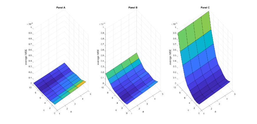
Figure 1: MISE values over 1000 simulated trajectories of the SV1F model with $\zeta=1$ (Panel A), $\zeta=2$ (Panel B) and $\zeta=3$ (Panel C).

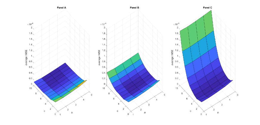
Figure 2: MISE values over 1000 simulated trajectories of the Heston model with $\zeta=1$ (Panel A), $\zeta=2$ (Panel B) and $\zeta=3$ (Panel C).

Figure 3: MIAE values over 1000 simulated trajectories of the SV1F model with $\zeta=1$ (Panel A), $\zeta=2$ (Panel B) and $\zeta=3$ (Panel C).

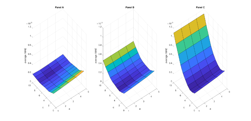
Figure 4: MIAE values over 1000 simulated trajectories of the Heston model with $\zeta=1$ (Panel A), $\zeta=2$ (Panel B) and $\zeta=3$ (Panel C).

	SV1F model		Heston model
noise-to-signal $\zeta$	optimal $(c,a)$	MISE	optimal $(c,a)$	MISE
$1$	$(7,0.2)$	$2.490\cdot 10^{-7}$	$(9,0.2)$	$9.082\cdot 10^{-8}$
$2$	$(3,0.1)$	$2.595\cdot 10^{-7}$	$(4,0.2)$	$1.376\cdot 10^{-7}$
$3$	$(2,0.1)$	$2.944\cdot 10^{-7}$	$(3,0.2)$	$1.513\cdot 10^{-7}$

Table 1: MISE-optimal selection of the pair $(c,a)$ for different values of the noise-to-signal ratio and resulting MISE values.

	SV1F model		Heston model
noise-to-signal $\zeta$	optimal $(c,a)$	MIAE	optimal $(c,a)$	MIAE
$1$	$(7,0.2)$	$1.638\cdot 10^{-4}$	$(7,0.3)$	$1.955\cdot 10^{-4}$
$2$	$(3,0.1)$	$2.036\cdot 10^{-4}$	$(4,0.3)$	$2.322\cdot 10^{-4}$
$3$	$(3,0.1)$	$2.267\cdot 10^{-4}$	$(3,0.3)$	$2.552\cdot 10^{-4}$

Table 2: MIAE-optimal selection of the pair $(c,a)$ for different values of the noise-to-signal ratio and resulting MIAE values.

5.3 Feasible selection of $N$ and $M$

In this subsection we introduce an adaptive method for the feasible selection of the pair $(N,M)$ in finite-sample applications. The method aims at optimizing the conditional MISE (c-MISE) of the Fourier spot volatility estimator under the constraint $M<N<n$, for the given available sample size $n$.

Define the c-MISE as

$$c\textit{-}MISE:=E^{\sigma}\left[\int_{0}^{T}\Big{(}\widetilde{\sigma}^{2}_{nNM}(t)-\sigma^{2}(t)\Big{)}^{2}dt\right],$$

where $E^{\sigma}$ denotes the conditional expectation w.r.t. the filtration generated by $(\sigma_{t})_{t\in[0,T]}$. As pointed out in [Zu and Boswijk, 2014, Section 3.4], the following decomposition holds:

$$c\textit{-}MISE=\int_{0}^{T}E^{\sigma}\left[\widetilde{\sigma}^{2}_{nNM}(t)-\sigma^{2}(t)\right]^{2}dt+\int_{0}^{T}Var^{\sigma}\left[\widetilde{\sigma}^{2}_{nNM}(t)-\sigma^{2}(t)\right]dt,$$

where $Var^{\sigma}$ denotes the conditional variance w.r.t. the filtration generated by $(\sigma_{t})_{t\in[0,T]}$. Under the assumptions of the rate-efficient Central Limit Theorem in (10), and after scaling the unit of time, for a sufficiently large $n$ the c-MISE is approximated by the conditional asymptotic integrated mean squared error (c-AMISE), which reads

$$c\textit{-}AMISE=\frac{M}{N}\,{2\over 3}\,\int_{0}^{T}\sigma^{4}(t)\,dt+\frac{1}{M}\,{T\over 3}\,\int_{0}^{T}\gamma^{2}(t)\,dt+\frac{M\,N}{n}\,{T\over 9}\,\xi\,\int_{0}^{T}\sigma^{2}(t)\,dt+\frac{N^{3}M}{n^{2}}\,{T^{3}\over{15}}\,\xi^{2}.$$ (13)

The c-AMISE in (13) depends on the integrated volatility $IV_{T}:=\int_{0}^{T}\sigma^{2}(t)dt$, the integrated quarticity $IQ_{T}:=\int_{0}^{T}\sigma^{4}(t)dt$, the integrated volatility-of-volatility $IVV_{T}:=\int_{0}^{T}\gamma^{2}(t)dt$ and the noise variance $\xi$. All these quantities can be estimated with high-frequency prices and thus the c-AMISE can be treated as observable. Specifically, for estimating $IV_{T}$, $IQ_{T}$ and $IVV_{T}$ we propose to use Fourier-transform based estimators. We refer the reader to, resp., [Mancino and Sanfelici, 2008], [Mancino and Sanfelici, 2012] and [Sanfelici et al., 2015] for the study of the finite-sample efficiency of the Fourier estimators of $IV_{T}$, $IQ_{T}$ and $IVV_{T}$ in the presence of noise and guidance on the practical implementation thereof with high-frequency prices. Moreover, for estimating $\xi$, we suggest to use the estimator studied in [Bandi and Russell, 2006, Section 3].

Let $n$ be fixed and, for brevity, denote the c-AMISE in (13) as a function of $(N,M)$ by $\Psi(N,M)$. Moreover, let $\widehat{\Psi}(N,M)$ indicate the estimator obtained by plugging the Fourier estimators of $IV_{T}$, $IQ_{T}$ and $IVV_{T}$, along with the estimator of $\xi$ by [Bandi and Russell, 2006], into (13), in place of the respective true latent quantities. Then, the feasible selection of $(N,M)$ for a given $n$ amounts to solving the constrained optimization problem

$$\min_{(N,M)\in S}\,\widehat{\Psi}(N,M),$$

where $S=\left[\underline{N},\overline{N}\right]\times\left[\underline{M},\overline{M}\right]\subset\mathbb{R}^{+}\times\mathbb{R}^{+}$ is such that $M<N<n$. To do so, we propose to use the following adaptive method, based on the gradient-descent algorithm (see, e.g., [Ruder, 2017]).

The implementation of the adaptive method for optimizing the pair $(N,M)$ requires the selection of the constraint region $S$ and the vector of optimization parameters $(\lambda,\vartheta,K)$. In this regard, given the sample size $n=23400$, corresponding to the sampling frequency $\rho(n)=1$ second, we set

$$S=\left[\lfloor{2}^{-1}n^{1/2}\rfloor,\lfloor 10\,n^{1/2}\rfloor\right]\times\left[\lfloor{10}^{-1}\,n^{1/4}\rfloor,\lfloor 2\,n^{1/4}\rfloor\right]$$ (14)

and

$$(\lambda,\vartheta,K)=(500\,\hat{\xi}^{-1},10^{-3},10^{5}).$$ (15)

Note that the choice of $S$ was performed rather conservatively, by allowing a fairly large range of variation for $N$ and $M$. Analogously, $\vartheta$ and $K$ were chosen conservatively to ensure that, trajectory-wise, the stopping rule $\delta_{k}<\vartheta$ was satisfied for some $k\leq K$. Moreover, particular attention was devoted to the choice of the learning rate $\lambda$, as the latter plays a crucial role in determining the accuracy of the gradient-descent algorithm, see [Ruder, 2017] and the references therein. In this regard, simulations suggest that a value inversely proportional to the (estimated) variance of the noise yields satisfactory results. In particular, after setting

$$\lambda=c_{\lambda}\,\hat{\xi}^{-1},$$

we numerically evaluated the efficiency of the adaptive method for different values of $c_{\lambda}$ in the region $[1,1000]$ and found that the MISE and MIAE values were optimized for $c_{\lambda}$ in a neighborhood of $500$, both in the case of the SV1F model and the Heston model, hence the selection of $\lambda$ in (15). As for robustness, MISE and MIAE values appeared to be rather stable for $c_{\lambda}\in[300,700]$, based on numerical evidence.

The performance of the feasible adaptive method in terms of MISE and MIAE is summarized in Table 3. Note that the latter is quite satisfactory, compared to the results of the unfeasible optimization exercise conducted in Subsection 5.2 (see Tables 1 and 2). In fact, MISE and MIAE values are smaller in Table 3. The better performance of the feasible adaptive method is explained by the fact that it optimizes the pair $(N,M)$ trajectory-wise.

	SV1F model		Heston model
noise-to-signal $\zeta$	MISE	MIAE	MISE	MIAE
$1$	$9.547\cdot 10^{-8}$	$1.216\cdot 10^{-4}$	$8.882\cdot 10^{-8}$	$1.913\cdot 10^{-4}$
$2$	$1.053\cdot 10^{-7}$	$1.335\cdot 10^{-4}$	$1.312\cdot 10^{-7}$	$2.300\cdot 10^{-4}$
$3$	$1.439\cdot 10^{-7}$	$1.480\cdot 10^{-4}$	$1.447\cdot 10^{-7}$	$2.507\cdot 10^{-4}$

Table 3: MISE and MIAE values produced by the feasible adaptive method for different values of the noise-to-signal ratio.

Remark 5.1

As pointed out in [Zu and Boswijk, 2014, Section 3.4], the c-MISE is a global measure of path-wise efficiency over the entire estimation interval. Accordingly, the adaptive method introduced in this section to minimize the c-MISE yields as an output a path-wise optimal value of the pair $(N,M)$ which is independent of the time instant $t\in[0,T]$. The results of the simulation study conducted in this section thus offer support to the efficiency of the Fourier estimator as a global estimator of the spot volatility path. This is line with the intrinsic global character of the Fourier spot volatility estimator, see [Malliavin and Mancino, 2009]. As already remarked in [Mancino and Recchioni, 2015], the global efficiency of the Fourier estimator may be relevant for financial applications (e.g., for the calibration of stochastic volatility models).

5.4 Performance comparison with alternative noise-robust estimators

This subsection illustrates a comparison of the finite-sample performance of the Fourier spot volatility estimator with that of alternative noise-robust spot volatility estimators, namely the Two-scale estimator by [Zu and Boswijk, 2014] and the Pre-averaging kernel estimator by [Figueroa and Wu, 2022]. We briefly recall the definitions of the two estimators.

The Two-scale estimator by [Zu and Boswijk, 2014] is defined as

$$\widetilde{\sigma}_{kh}^{2}(t):=\frac{1}{h}\sum_{t\leq t_{i}\leq t+h}\frac{(\widetilde{p}_{t_{i+k}}-\widetilde{p}_{t_{i}})^{2}}{k}-\frac{\bar{n}}{n}\frac{1}{h}\sum_{t\leq t_{i}\leq t+h}\delta_{i}(\widetilde{p})^{2},$$ (16)

where $\bar{n}=\frac{nh-k+1}{kh}$, $k=\lfloor c_{k}n^{2/3}\rfloor$ and $h=c_{h}n^{-1/6}$. The implementation of (16) then requires the selection of the constants $c_{k}$ and $c_{h}$. For this task, we followed [Zu and Boswijk, 2014, Section 3.4].

The pre-averaging kernel estimator by [Figueroa and Wu, 2022] reads

$$\widetilde{\sigma}_{km}^{2}(t):=\frac{1}{\phi_{k}(g)}\sum_{i=1}^{n-k+1}\frac{1}{m\Delta_{n}}K\left(\frac{t_{i}-t}{m\Delta_{n}}\right)\left(\bar{P}_{i}^{2}-\frac{1}{2}\widehat{P}_{i}\right),$$ (17)

where: $\Delta_{n}=T/n$, $k=\lfloor 1/\left(c_{k}\sqrt{\Delta_{n}}\right)\rfloor$ and $m=c_{m}\Delta_{n}^{-3/4}$; $K$ is a kernel function satisfying Assumption 2 of [Figueroa and Wu, 2022]; $g$ is a real-valued weight function on $[0,1]$ continuous and piece-wise $C^{1}$ with a piece-wise Lipschitz derivative $g^{\prime}$; moreover $g(0)=g(1)=0$, $\int_{0}^{1}g^{2}(s)ds=1$; finally,

$$\bar{P}_{i}=-\sum_{j=1}^{k}\left(g\left(\frac{j}{k}\right)-g\left(\frac{j-1}{k}\right)\right)\widetilde{p}_{i+j-2},\quad\widehat{P}_{i}=\sum_{j=1}^{k}\left(g\left(\frac{j}{k}\right)-g\left(\frac{j-1}{k}\right)\right)^{2}\delta_{i+j-2}(\widetilde{p})^{2},\quad\phi_{k}(g)=\sum_{j=1}^{k}g\left(\frac{j}{k}\right)^{2}.$$

To apply the estimator in (17), one then needs to select a kernel function $K$ and a pre-averaging function $g$, along with the constants $c_{k}$ and $c_{m}$. Based on the discussion in [Figueroa and Wu, 2022, Section 3], we selected $K(x)=\frac{1}{2}\textrm{e}^{-|x|}$. Further, we chose $c_{k}$ and $c_{m}$ in accordance with the formulas derived by the authors to optimize the integrated asymptotic variance (see also Remark 4.1 in [Figueroa and Wu, 2022]). As for the function $g$, we selected $g(x)=x\wedge(1-x)$, as in [Jacod et al., 2009].

Tables 4 and 5 summarize the results of the comparative performance study.

	SV1F model		Heston model
noise-to-signal $\zeta$	MISE	MIAE	MISE	MIAE
$1$	$4.986\cdot 10^{-7}$	$3.297\cdot 10^{-4}$	$3.951\cdot 10^{-7}$	$5.247\cdot 10^{-4}$
$2$	$7.016\cdot 10^{-7}$	$3.304\cdot 10^{-4}$	$9.326\cdot 10^{-7}$	$7.071\cdot 10^{-4}$
$3$	$8.045\cdot 10^{-7}$	$2.864\cdot 10^{-4}$	$1.179\cdot 10^{-6}$	$7.777\cdot 10^{-4}$

Table 4: Two-scale estimator (16): MISE and MIAE values for different values of the noise-to-signal ratio.

	SV1F model		Heston model
noise-to-signal $\zeta$	MISE	MIAE	MISE	MIAE
$1$	$2.146\cdot 10^{-7}$	$1.898\cdot 10^{-4}$	$1.928\cdot 10^{-7}$	$3.105\cdot 10^{-4}$
$2$	$2.379\cdot 10^{-7}$	$1.916\cdot 10^{-4}$	$1.944\cdot 10^{-7}$	$3.176\cdot 10^{-4}$
$3$	$2.382\cdot 10^{-7}$	$1.939\cdot 10^{-4}$	$2.191\cdot 10^{-7}$	$3.366\cdot 10^{-4}$

Table 5: Pre-averaging kernel estimator (17): MISE and MIAE values for different values of the noise-to-signal ratio.

The comparison of Tables 4 and 5 with Table 3 suggests that the Fourier estimator yields the lowest MISE and MIAE values under both parametric settings adopted and for each of the three noise-to-signal ratios employed. Moreover, the Pre-averaging estimator appears to produce lower MISE and MIAE values compared to the Two-scale estimator in each scenario considered. This is coherent with the numerical results illustrated in [Figueroa and Wu, 2022, Section 4.6]. However, it is worth noticing that the performance gap observed in the simulation study between the Fourier and the Pre-averaging estimators appears to decrease as the noise-to-signal ratio is increased, in terms of both MISE and MIAE.

Overall, we observe that the numerical findings of this subsection robustify the numerical evidence produced in [Mancino and Recchioni, 2015] by taking into account also the estimator by [Figueroa and Wu, 2022] for the performance comparison. Furthermore, it is worth noticing that the performance ranking of spot volatility estimators obtained here is coherent with the ranking obtained in the simulation study by [Mariotti et al., 2022], where the data-generating process is the limit order book simulator by [Huang et al., 2015].

6 Empirical study

In this section we illustrate a study on the accuracy of the Fourier spot volatility estimator with S&P500 high-frequency trade prices, sampled over the period March, 2018 - April, 2018.

The accuracy of spot volatility estimates can be investigated empirically by testing the distribution of the reconstructed standardized log-return, see [Mancino and Recchioni, 2015, Section 4]. Define the standardized log-return on $[t,t+h]$, $h>0$, as

$$z_{h}(t):=\frac{r_{h}(t)}{\sqrt{\sigma^{2}(t)\,h}},$$ (18)

where $r_{h}(t):=p(t+h)-p(t)$. Moreover, denote by $z_{h}^{F}(t)$ the reconstructed standardized log-return, obtained by replacing $\sigma^{2}(t)$ in (18) with the Fourier estimate thereof. Under Assumption (A.I), if the interval $h$ is sufficiently small, the sequence $\{z_{h}(t)\}_{t\in\tau}$, $\tau=\{0,h,2h,...,(\lfloor T/h\rfloor-1)h\}$, approximates a sequence of i.i.d. standard Normal random variables. By testing the empirical distribution of the reconstructed standardized log-returns $\{z^{F}_{h}(t)\}_{t\in\tau}$ for Normality, one can then obtain insight on the accuracy of Fourier spot volatility estimates.

The estimation of the spot volatility was conducted on the daily horizon, that is, on the time interval between 9:30 a.m. and 4:00 p.m. As we measured time in days, the corresponding value of $T$ was set equal to $1$. For the implementation of the Fourier estimator, we used the sampling frequency $\rho(n)=1$ second, corresponding to $n=23400$. As for the selection of $N$ and $M$, we employed the adaptive method described in Subsection 5.3 and, based on the recommendation from the simulation study, we made the choice of the rectangle $S$ and the optimization parameters $\lambda,\vartheta,K$ as in, respectively, (14) and (15). Note that, on average, the adaptive method lead to the selection of $N=305.48$ and $M=6.94$.

Days with price jumps were not considered. In this regard, after applying the jump test by [Lee and Mykland, 2008] at the 95% confidence level, we detected the presence of intraday jumps only on March 14th and thus the corresponding daily sub-sample was discarded. Overnight returns, that is, the difference between the opening log-price and the closing log-price of the previous day, were not employed in the estimation, as they typically contain jumps due to the fact that news releases usually take place when the market is closed. In fact, the test by [Lee and Mykland, 2008] at the 95% confidence level detected jumps in correspondence of overnight returns for approximately 40% of the days of the 2-month sample object of study. Overall, we obtained $41$ spot volatility daily paths.

In order to test the distribution of the reconstructed standardized log returns, one needs to select a value for the interval $h$ which is, at the same time, small enough to satisfactorily approximate the standard Gaussian distribution and large enough to make the impact of micro-structure noise negligible. Based on the application of the noise-detection test by [Aït-Sahalia and Xiu, 2019], we selected $h$ equal to $5$ minutes. Accordingly, Fourier estimates of the spot volatility were obtained on the equally-spaced grid with mesh size equal to 5 minutes. However, it is worth stressing that the Fourier method allows selecting an arbitrary grid for the estimation of the volatility path and that the selection of the 5-minute grid is only convenient for the purpose of the testing of the reconstructed standardized log-return distribution. The sequence of the reconstructed daily volatility paths is displayed in Figure 5.

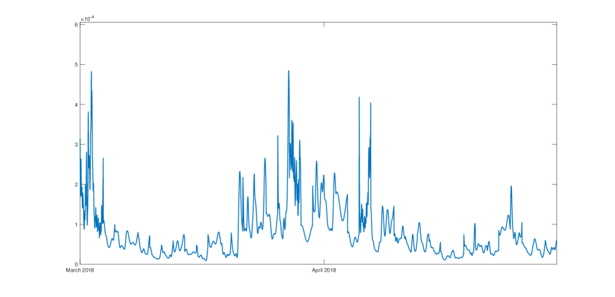
Figure 5: S&P500 (March, 2018 - April, 2018): sequence of the reconstructed daily volatility paths on the 5-minute grid.

We applied the Jarque-Bera test (see [Jarque and Bera, 1987]) to the $41$ daily samples of reconstructed standardized log-returns. At the 95% confidence level, the null hypothesis of Gaussianity was never rejected. The average p-value was equal to $0.374$. Moreover, Table 6 reports the averages and standard deviations, over the 41 daily samples analyzed, of the sample mean, variance, skewness and kurtosis of the reconstructed standardized log-returns. The averages are very close to the theoretical moments of a standard Normal, while the standard deviations are relatively small. Overall, the results of the Jarque-Bera test, along with the empirical evidence on the sample moments, suggest that the daily empirical distributions of the reconstructed standardized log-returns approximate a standard normal quite well, thereby supporting the accuracy of the Fourier spot volatility estimates obtained.

	average	std. dev.
mean	-0.005	0.132
variance	1.008	0.182
skewness	0.006	0.222
kurtosis	2.940	0.268

Table 6: S&P500 (March, 2018 - April, 2018): averages and standard deviations, over the 41 daily samples analyzed, of the sample statistics of the reconstructed standardized log-returns.

7 Conclusions

We have proved two rate-optimal central limit theorems for the Fourier estimator of the spot volatility both in the absence and in the presence of additive microstructure noise. In the absence of noise, our result completes the asymptotic theory presented in [Mancino and Recchioni, 2015], where the rate is slightly sub-optimal under more general hypotheses on the volatility process. Additionally, we have derived a feasible adaptive method for the optimal selection of the parameters involved in the implementation and provided numerical results which support its accuracy. Finally, we offered support to the reliability of the adaptive method for practical applications via an empirical study, conducted with a short sample of S&P500 high-frequency prices.

8 Appendix A

Please contact the authors for the proofs.

9 Appendix B

This Appendix resumes some results about the rescaled Dirichlet kernel, defined as

$$D_{N}(x):={1\over{2N+1}}\sum_{|k|\leq N}e^{{\rm i}kx}={1\over{2N+1}}{\sin((2N+1)x/2)\over{\sin(x/2)}}$$ (19)

and the Fejér kernel, defined as

$$F_{M}(x):=\sum_{|k|\leq M}\left(1-{|k|\over{M+1}}\right)\,e^{{\rm i}kx}={1\over{M+1}}\left({\sin((M+1)x/2)\over{\sin(x/2)}}\right)^{2}.$$ (20)

Lemma 9.1

i) For any $M$,

$$\int_{-\pi}^{\pi}F_{M}(x)dx=2\pi.$$

Moreover, under the assumption $\lim_{n,M\to\infty}{M^{\tau}\over n}=a$, for a constant $a>0$ and for some $\tau>1$, it holds:

$$\lim_{n,M\to\infty}\int_{-\pi}^{\pi}F_{M}(\varphi_{n}(x))dx=2\pi$$

and, in particular,

$$\left|\int_{-\pi}^{\pi}F_{M}(\varphi_{n}(x))dx-\int_{-\pi}^{\pi}F_{M}(x)dx\right|\leq C{M\over n}.$$

ii) For any $M\geq 1$,

$$\int_{2\pi\over{M+1}}^{\pi}F_{M}(x)dx\leq{C\over M}.$$

iii) Under the assumption $\lim_{n,M\to\infty}{M^{\tau}\over n}=a$, for a constant $a>0$ and for some $\tau>1$, it holds:

$$\lim_{M\to\infty}\int_{-\pi}^{\pi}{1\over M}F^{2}_{M}(x)dx=\lim_{M,n\to\infty}\int_{-\pi}^{\pi}{1\over M}F^{2}_{M}(\varphi_{n}(x))dx={4\pi\over 3}.$$ (21)

iv) If $\lim_{n,M\to\infty}{M^{\tau}\over n}=a$, for a constant $a>0$ and for some $\tau>1$, and $f$ is Hölder continuous with parameter $\alpha\in(0,1]$, then

$$\lim_{n,M\to\infty}{{1\over M}}\int_{-\pi}^{\pi}F_{M}^{2}(x-\varphi_{n}(y))f(y)dy=\lim_{M\to\infty}\int_{-\pi}^{\pi}{1\over M}F_{M}^{2}(x-y)f(y)dy={4\pi\over 3}f(x).$$ (22)

Proof. See [Cuchiero and Teichmann, 2015, Lemma 5.1].

Remark 9.2

As observed in [Cuchiero and Teichmann, 2015] Remark 5.2, all above results similarly hold true on $[0,T]$.

Lemma 9.3

Suppose that $\lim_{n,M\to\infty}{M^{\tau}\over n}=a$, for some constant $a>0$ and $\tau>1$. Then, it holds that:

$$\lim_{n,M\to\infty}\int_{-\pi}^{\pi}\frac{1}{M^{3}}|F^{\prime}_{M}(\varphi_{n}(x))|^{2}\,dx=\lim_{M\to\infty}\int_{-\pi}^{\pi}\frac{1}{M^{3}}|F^{\prime}_{M}(x)|^{2}\,dx=\frac{2}{15}\pi,$$ (23)

$$\lim_{n,M\to\infty}\int_{-\pi}^{\pi}\frac{1}{M^{5}}|F^{\prime\prime}_{M}(\varphi_{n}(x))|^{2}\,dx=\lim_{M\to\infty}\int_{-\pi}^{\pi}\frac{1}{M^{5}}|F^{\prime\prime}_{M}(x)|^{2}\,dx=\frac{4}{105}\pi.$$ (24)

Proof. See [Toscano et al., 2022, Lemma 8.1].

Lemma 9.4

i) If $\lim_{n,N\to\infty}{N\over n}=c>0$, then for any $p>1$ there exists a constant $C_{p}$ such that

$$\lim_{n,N\to\infty}\,n\sup_{x\in[0,2\pi]}\int_{0}^{2\pi}D^{p}_{N}(\varphi_{n}(x)-\varphi_{n}(y))dy\leq C_{p}.$$

ii) If $\lim_{n,N\to\infty}{N\over n}=c>0$, it holds that

$$\lim_{n,N\to\infty}n\,\int_{0}^{x}D^{2}_{N}(\varphi_{n}(x)-\varphi_{n}(y))dy=\pi(1+2K(2c))$$

and, for any $\alpha$-Hölder continuous function $f$ with $\alpha\in(0,1]$,

$$\lim_{N,n\to\infty}n\int_{0}^{x}D^{2}_{N}(\varphi_{n}(x)-\varphi_{n}(y))f(y)dy=\pi(1+2K(2c))\,f(x),$$

where

$$K(c):=\frac{1}{2c^{2}}r(c)(1-r(c)),$$

being $r(c)=c-[c]$, with $[c]$ denoting the integer part of $c$.

iii) If $\lim_{n,N\to\infty}{N\over n}=c>0$, then for any $s\in[0,2\pi)$ and for any $\varepsilon>0$,

$$\lim_{n,N\to\infty}\ n\int_{0}^{x-\varepsilon}D^{2}_{N}(\varphi_{n}(x)-\varphi_{n}(y))dy=0.$$

Proof. See [Clement and Gloter, 2011, Lemma 3].

Lemma 9.5

If $\lim_{N,n\to\infty}{N^{\tau}\over n}=c$, for a constant $c>0$ and some $\tau>1$, then

$$\lim_{n,N\to\infty}N\,\int_{0}^{x}D^{2}_{N}(\varphi_{n}(x)-\varphi_{n}(y))dy=\lim_{N\to\infty}{N}\,\int_{0}^{x}D^{2}_{N}(x-y)dy={\pi\over 2}.$$

Proof. See [Cuchiero and Teichmann, 2015, Lemma 5.1], using the fact that $D_{N}^{2}(x)=(2N+1)^{-1}F_{2N}(x)$.

Lemma 9.6

Under the condition $\lim_{N,n\to\infty}{N^{\tau}\over n}=c$, for a constant $c>0$ and some $\tau>1$, it holds:

$$i)\,\,\,\lim_{n,N\to\infty}{1\over N}\int_{0}^{2\pi}|D^{\prime}_{N}(\varphi_{n}(x))|^{2}dx=\lim_{N\to\infty}{1\over N}\int_{0}^{2\pi}|D^{\prime}_{N}(x)|^{2}dx={\pi\over 3}.$$

$$ii)\,\,\,\lim_{n,N\to\infty}{1\over{N^{3}}}\int_{0}^{2\pi}|D^{\prime\prime}_{N}(\varphi_{n}(x))|^{2}dx=\lim_{N\to\infty}{1\over{N^{3}}}\int_{0}^{2\pi}|D^{\prime\prime}_{N}(x)|^{2}dx={\pi\over 5}.$$

Proof. For i) see [Mancino and Toscano, 2022]. As for ii), it holds that:

$$\frac{1}{N^{3}}\int_{0}^{2\pi}\left|D^{\prime\prime}_{N}(x)\right|^{2}dx=\frac{1}{N^{3}}\frac{2\pi}{\left(2N+1\right)^{2}}\sum_{|k|\leq N}k^{4}=\frac{2\pi}{15}\frac{N(N+1)(3N^{2}+3N-1)}{N^{3}(2N+1)}\rightarrow\frac{\pi}{5}.$$

References

- [Aït-Sahalia and Jacod, 2014] Aït-Sahalia, Y. and Jacod, J. (2014). High-frequency financial econometrics. Princeton University Press.
- [Aït-Sahalia and Xiu, 2019] Aït-Sahalia, Y. and Xiu, D. (2019). A Hausman test for the presence of noise in high frequency data. Journal of Econometrics, 211(1), 176–205.
- [Andersen et al., 2005] Andersen, T.G., Bollerslev, T., Diebold, F.X. and Labys, P. (2001). Modeling and forecasting realized volatility. Econometrica, 71(2), 529–626.
- [Bandi and Russell, 2006] Bandi, F.M. and Russell, J.R. (2006). Separating microstructure noise from volatility. Journal of Financial Economics, 79(3), 655–692.
- [Barndorff-Nielsen et al., 2008] Barndorff-Nielsen, O.E., Hansen, P.R., Lunde, A. and Shephard, N. (2008). Designing realised kernels to measure the ex-post variation of equity prices in the presence of noise. Econometrica, 76(6), 1481–1536.
- [Barucci and Renò, 2002] Barucci, E. and Renò, R. (2002). On measuring volatility and the GARCH forecasting performance. Journal of International Financial Markets, Institutions and Money, 12(3), 183–200.
- [Clement and Gloter, 2011] Clement, E. and Gloter, A. (2011). Limit theorems in the Fourier transform method for the estimation of multivariate volatility. Stochastic Processes and their Applications, 121(5), 1097–1124.
- [Cuchiero and Teichmann, 2015] Cuchiero, C. and Teichmann, J. (2015). Fourier transform methods for pathwise covariance estimation in the presence of jumps. Stochastic Processes and Their Applications, 125(1), 116–160.
- [Figueroa and Li, 2020] Figueroa-López, J.E. and Li, C. (2020). Optimal kernel estimation of spot volatility of stochastic differential equations. Stochastic Processes and their Applications, 130(8), 4693–4720.
- [Figueroa and Wu, 2022] Figueroa-López, J.E. and Wu, B. (2022). Kernel estimation of spot volatility with microstructure noise using pre-averaging. https://arxiv.org/pdf/2004.01865.pdf.
- [Hansen and Lunde, 2006] Hansen, P.R. and Lunde A. (2006). Realized variance and market microstructure noise. Journal of Business and Economic Statistics, 24(2), 127–218.
- [Heston, 1993] Heston, S. L. (1993). A closed-form solution for options with stochastic volatility with applications to bond and currency options. Review of Financial Studies, 6(2), 327-343.
- [Huang and Tauchen, 2005] Huang, X. and Tauchen, G. (2005). The relative contribution of jumps to total price variance. Journal of Financial Econometrics, 3(4), 456–499.
- [Huang et al., 2015] Huang, W., Lehalle, C.A. and Rosenbaum, M. (2015). Simulating and analyzing order book data: the queue-reactive model. Journal of the American Statistical Association, 110(509), 107–122.
- [Jacod, 1997] Jacod, J. (1997). On continuous conditional Gaussian martingales and stable convergence in law. Séminarire de Probabilités XXXI in Lecture Notes in Mathematics, Springer, 1655, 232–246.
- [Jacod et al., 2009] Jacod, J., Li, Y., Mykland, P., Podolskij, M. and Vetter, M. (2009). Microstructure noise in the continuous case: The pre-averaging approach. Stochastic Processes and their Applications, 119(7), 2249–2276.
- [Jacod and Protter, 1998] Jacod, J. and Protter, P. (1998). Asymptotic error distributions for the Euler method for stochastic differential equations. Annals of Probability, 26(1), 267–307.
- [Jarque and Bera, 1987] Jarque, C.M. and Bera, A.K. (1987). A test for normality of observations and regression residuals. International Statistical Review, 55(2), 163–172 .
- [Kristensen, 2010] Kristensen, D. (2010). Non-parametric filtering of the realized spot volatility: a kernel-based approach. Econometric Theory, 26(1), 60–93.
- [Lee and Mykland, 2008] Lee, S. and Mykland, P.A. (2008). Jumps in financial markets: a new nonparametric test and jump dynamics. The Review of Financial Studies, 21(6), 2535–2563.
- [Malliavin and Mancino, 2002] Malliavin, P. and Mancino, M.E. (2002). Fourier series method for measurement of multivariate volatilities. Finance and Stochastics, 6(1), 49–61.
- [Malliavin and Mancino, 2009] Malliavin, P. and Mancino, M.E. (2009). A Fourier transform method for non-parametric estimation of volatility. The Annals of Statistics, 37(4), 1983–2010.
- [Mancini et al., 2015] Mancini, C., Mattiussi, V. and Renó, R. (2015). Spot volatility estimation using delta sequences. Finance and Stochastics, 19(2), 261–293.
- [Mancino et al., 2017] Mancino, M.E., Recchioni, M.C. and Sanfelici, S. (2017). Fourier-Malliavin volatility estimation. Theory and practice. Spinger.
- [Mancino and Recchioni, 2015] Mancino, M.E. and Recchioni, M.C. (2015). Fourier spot volatility estimator: asymptotic normality and efficiency with liquid and illiquid high-frequency data. PLOS ONE, 10(9).
- [Mancino and Sanfelici, 2008] Mancino, M.E. and Sanfelici, S. (2008). Robustness of Fourier estimator of integrated volatility in the presence of microstructure noise. Computational Statistics and Data Analysis, 56(2), 2966–2989.
- [Mancino and Sanfelici, 2011] Mancino, M.E. and Sanfelici, S. (2011). Estimating covariance via Fourier method in the presence of asynchronous trading and microstructure noise. Journal of Financial Econometrics, 9(2), 367–408.
- [Mancino and Sanfelici, 2012] Mancino, M.E. and Sanfelici, S. (2012). Estimation of quarticity with high-frequency data (2012). Quantitative Finance, 12(4), 607–622.
- [Mancino and Toscano, 2022] Mancino, M.E. and Toscano, G. (2022). Rate-efficient asymptotic normality for the Fourier estimator of the leverage process. Statistics and Its Interface, 15(1), 73–89.
- [Mariotti et al., 2022] Mariotti, T., Lillo, F. and Toscano, G. (2022). From zero-intelligence to queue-reactive: limit order book modeling for high-frequency volatility estimation and optimal execution. https://arxiv.org/pdf/2202.12137.pdf.
- [Nielsen and Frederiksen, 2006] Nielsen, M.O. and Frederiksen, P.H. (2006). Finite-sample accuracy and choice of sampling frequency in integrated volatility estimation. Journal of Empirical Finance, 15(2), 265–286.
- [Park et al., 2016] Park, S., Hong, S.Y. and Linton, O. (2016). Estimating the quadratic covariation matrix for asynchronously observed high-frequency stock returns corrupted by additive measurement error. Journal of Econometrics, 191(2), 325–347.
- [Ruder, 2017] Ruder, S. (2017). An overview of gradient descent optimization algorithms. https://arxiv.org/pdf/1609.04747.pdf.
- [Sanfelici et al., 2015] Sanfelici, S., Curato, I.V. and Mancino, M.E. (2015). High-frequency volatility of volatility estimation free from spot volatility estimates. Quantitative Finance, 15(8), 1331–1345.
- [Toscano et al., 2022] Toscano, G., Livieri, G., Mancino, M.E. and Marmi, S. (2022). Volatility of volatility estimation: central limit theorems for the Fourier transform estimator and empirical study of the daily time series stylized facts. https://arxiv.org/pdf/2112.14529.pdf.
- [Zhou, 1996] Zhou, B. (1996). High-frequency data and volatility in foreign-exchange rates. Journal of Business and Economic Statistics, 14(1), 45–52.
- [Zu and Boswijk, 2014] Zu, Y. and Boswijk, H.P. (2014). Estimating spot volatility with high-frequency financial data. Journal of Econometrics, 181(2), 117–135.