Learning Symbolic Model-Agnostic Loss Functions via Meta-Learning

Abstract

In this paper, we develop upon the emerging topic of loss function learning, which aims to learn loss functions that significantly improve the performance of the models trained under them. Specifically, we propose a new meta-learning framework for learning model-agnostic loss functions via a hybrid neuro-symbolic search approach. The framework first uses evolution-based methods to search the space of primitive mathematical operations to find a set of symbolic loss functions. Second, the set of learned loss functions are subsequently parameterized and optimized via an end-to-end gradient-based training procedure. The versatility of the proposed framework is empirically validated on a diverse set of supervised learning tasks. Results show that the meta-learned loss functions discovered by the newly proposed method outperform both the cross-entropy loss and state-of-the-art loss function learning methods on a diverse range of neural network architectures and datasets. We make our code available at *retracted*.

1 Introduction

The field of learning-to-learn or meta-learning has been an area of increasing interest to the machine learning community in recent years [1, 2]. In contrast to conventional learning approaches, which learn from scratch using a static learning algorithm, meta-learning aims to provide an alternative paradigm whereby intelligent systems leverage their past experiences on related tasks to improve future learning performances [3]. This paradigm has provided an opportunity to utilize the shared structure between problems to tackle several traditionally very challenging deep learning problems in domains where both data and computational resources are limited [4, 5].

Many meta-learning approaches have been proposed for optimizing various components of deep neural networks. For example, early research on the topic explored using meta learning for generating learning rules [6, 7, 8, 9]. More recent research has extended itself to learning everything from activation functions [10], shared parameter/weight initializations [11, 12, 13, 14], and neural network architectures [15, 16, 17, 18] to whole learning algorithms from scratch [19, 20] and many more.

However, one component that has been overlooked until very recently is the loss function [21]. Typically in deep learning, neural networks are trained through the backpropagation of gradients originating from a handcrafted and manually selected loss function [22]. One significant drawback of this approach is that traditionally loss functions have been designed with task-generality in mind, i.e. large classes of tasks in mind, but the system itself is only concerned with a single instantiation or small subset of that class. However, as shown by the No Free Lunch Theorems [23] no algorithm is able to do better than a random strategy in expectation — this suggests that specialization to a subclass of tasks is in fact the only way that performance can be improved in general.

Given this importance, the prototypical approach of selecting a loss function heuristically from a modest set of handcrafted loss functions should be reconsidered in favor of a more principled data-informed approach. The new and emerging subfield of loss function learning offers an alternative to this, which instead aims to leverage task-specific information and past experiences to infer and discover highly performant loss functions directly from the data. Initial approaches to loss function learning have shown promise in improving various aspects of deep neural networks training. However, they have several key issues and limitations which must be addressed for meta-learned loss functions to become a more desirable alternative than handcrafted loss functions.

In particular, many loss function learning approaches use a parametric loss representation such as a neural network [24] or Taylor polynomial [25, 26, 27], which is limited as it imposes unnecessary assumptions and constraints on the structure of the learned loss function. However, the current non-parametric alternative to this is to use a two-stage discovery and optimization process, which infers both the loss function structure and parameters simultaneously using genetic programming and covariance matrix adaptation [28], and quickly become intractable for large-scale optimization problems. Subsequent work [29, 30] has attempted to address this issue; however, they crucially omit the optimization stage, which is known to produce sub-optimal performance.

This paper aims to resolve these issues through a newly proposed framework called Evolved Model-Agnostic Loss (EvoMAL), which meta-learns non-parametric symbolic loss functions via a hybrid neuro-symbolic search approach. The newly proposed framework aims to resolve the limitations of past approaches to loss function learning by combining genetic programming [31] with an efficient gradient-based local-search procedure [32, 33]. This unifies two previously divergent lines of research on loss function learning, which prior to this method, exclusively used either a gradient-based or an evolution-based approach.

This work innovates on the prior loss function learning approaches by introducing the first computationally tractable approach to optimizing symbolic loss functions. Consequently, improving the scalability and performance of symbolic loss function learning algorithm. Furthermore, unlike prior approaches, the proposed framework is both task and model-agnostic, as it can be applied to learning algorithm trained with a gradient descent style procedure and is compatible with different model architectures. This branch of general-purpose loss function learning algorithms provides a new powerful avenue for improving a neural network’s performance, which has until recently not been explored.

The performance of EvoMAL is assessed on a diverse range of datasets and neural network architectures in the direct learning and transfer learning settings, where the empirical performance is compared with the ubiquitous cross-entropy loss and other state-of-the-art loss function learning methods. Finally, an analysis of the meta-learned loss functions produced by EvoMAL is presented, where several reoccurring trends are identified in both the shape and structure. Further analysis is also given to show why meta-learned loss functions are so performant through 1) examining the loss landscapes of the meta-learned loss functions and 2) investigating the relationship between the base learning rate and the meta-learned loss functions.

1.1 Contributions:

The key contributions of this work are as follows:

• We propose a new task and model-agnostic search space and a corresponding search algorithm for meta-learning interpretable symbolic loss functions.

• We demonstrate a simple transition procedure for converting expression tree-based symbolic loss functions into gradient trainable loss networks.

• We utilize the new loss function representation to integrate the first computationally tractable approach to optimizing symbolic loss functions into the framework.

• We evaluate the proposed framework by performing the first-ever comparison of existing loss function learning techniques in both direct learning and transfer learning settings.

• We analyze the meta-learned loss functions to highlight key trends and explore why meta-learned loss functions are so performant.

2 Background and Related Work

The goal of loss function learning in the meta-learning context is to learn a loss function $\mathcal{M}_{\phi}$ with parameters $\phi$, at meta-training time over a distribution of tasks $p(\mathcal{T})$. A task is defined as a set of input-output pairs $\mathcal{T}=\{(x_{1},y_{1}),\dots,(x_{N},y_{N})\}$, and multiple tasks compose a meta-dataset $\mathcal{D}=\{\mathcal{T}_{1},\dots,\mathcal{T}_{M}\}$. Then, at meta-testing time the learned loss function $\mathcal{M}_{\phi}$ is used in place of a traditional loss function to train a base learner, e.g. a classifier or regressor, denoted by $f_{\theta}(x)$ with parameters $\theta$ on a new unseen task from $p(\mathcal{T})$. In this paper, we constrain the selection of base learners to models trainable via a gradient descent style procedures such that we can optimize weights $\theta$ as follows:

$$\theta_{new}=\theta-\alpha\nabla_{\theta}\mathcal{M}_{\phi}(y,f_{\theta}(x))$$ (1)

Several approaches have recently been proposed to accomplish this task, and an observable trend is that most of these methods fall into one of the following two key categories.

2.1 Gradient-Based Approaches

Gradient-based approaches predominantly aim to learn a loss function $\mathcal{M}$ through the use of a meta-level neural network to improve on various aspects of the training. For example, in [34, 35], differentiable surrogates of non-differentiable performance metrics are learned to reduce the misalignment problem between the performance metric and the loss function. Alternatively, in [36, 37, 38, 39, 24, 40, 41, 42], loss functions are learned to improve sample efficiency and asymptotic performance in supervised and reinforcement learning, while in [43, 44, 45, 27], they improved on the robustness of a model.

While the aforementioned approaches have achieved some success, they have notable limitations. The most salient limitation is that they a priori assume a parametric form for the loss functions. For example, in [24] and [46], it is assumed that the loss functions take on the parametric form of a two hidden layer feed-forward neural network with 50 nodes in each layer and ReLU activations. However, such an assumption imposes a bias on the search, often leading to an over parameterized and sub-optimal loss function. Another limitation is that these approaches often learn black-box (sub-symbolic) loss functions, which is not ideal, especially in the meta-learning context where post hoc analysis of the learned component is crucial, before transferring the learned loss function to new unseen problems at meta-testing time.

2.2 Evolution-Based Approaches

A promising alternative paradigm is to use evolution-based methods to learn $\mathcal{M}_{\phi}$, favoring their inherent ability to avoid local optima via maintaining a population of solutions, their ease of parallelization of computation across multiple processors, and their ability to optimize for non-differentiable functions directly. Examples of such work include [25] and [26], which both represent $\mathcal{M}_{\phi}$ as parameterized Taylor polynomials optimized with covariance matrix adaptation evolutionary strategies (CMA-ES). These approaches successfully derive interpretable loss functions, but similar to previously, they also assume the parametric form via the degree of the polynomial.

To resolve the issue of having to assume the parametric form of $\mathcal{M}_{\phi}$, another avenue of research first presented in [28] investigated the use of genetic programming (GP) to learn the structure of $\mathcal{M}_{\phi}$ in a symbolic form before applying CMA-ES to optimize the parameterized loss. The proposed method was effective at learning performant loss functions and clearly demonstrated the importance of local-search. However, the method had intractable computational costs as using a population-based method (GP) with another population-based method (CMA-ES) resulted in a significant expansion in the number of evaluations at meta-training time, hence it needing to be run on a supercomputer in addition to using a truncated number of training steps.

Subsequent work in [29] and [30] reduced the computational cost of GP-based loss function learning approaches by proposing time saving mechanisms such as: rejection protocols, gradient-equivalence-checking, convergence property verification and model optimization simulation. These methods successfully reduced the wall-time of GP-based approaches; however, both papers omit the use of local-search strategies, which is known to cause sub-optimal performance when using GP [47, 48, 49]. Furthermore, neither method is task and model-agnostic, limiting their utility to a narrow set of domains and applications.

3 Evolved Model-Agnostic Loss

In this work, a novel hybrid neuro-symbolic search approach named Evolved Model-Agnostic Loss (EvoMAL) is proposed, which consolidates and extends past research on the topic of loss function learning. The proposed method learns performant and interpretable symbolic loss functions by inferring both the structure and the weights/coefficients directly from the data. The evolution-based technique GP [31] is used to solve the discrete problem of deriving the symbolic structure of the learned loss functions, while unrolled differentiation [50, 51, 52, 32], a gradient-based technique previously used in Meta-Learning via Learned Loss (ML³) [24], and sometimes referred to as Generalized Inner Loop Meta-Learning [33], is used to solve the continuous problem of optimizing their weights/coefficients.

3.1 Offline Loss Function Learning Setup

EvoMAL is a new approach to offline loss function learning, a meta-learning paradigm concerned with learning new and performant loss functions that can be used as a drop-in replacement for a prototypical handcrafted loss function such as the squared loss for regression or cross-entropy loss for classification [53, 54]. Offline loss function learning follows a conventional offline meta-learning setup, which partitions the learning into two sequential phases: meta-training and meta-testing.

3.1.1 Meta-Training Phase

The meta-training phase in EvoMAL is formulated as a bilevel optimization problem, where the goal of the outer optimization is to meta-learn a performant loss function $\mathcal{M}_{\phi}$ minimizing the average task loss $\mathcal{L}_{\mathcal{T}}$ (the meta-objective) across $m$ related tasks, where $\mathcal{L}_{\mathcal{T}}$ is selected based on the desired task. The inner optimization uses $\mathcal{M}_{\phi}$ as the base loss function to train the base model parameters $\theta$. Formally, the meta-training phase of EvoMAL is defined as follows:

$$\begin{split}\mathcal{M}_{\phi}^{*}&=\operatorname*{arg\,min}_{\mathcal{M}_{\phi}}\frac{1}{m}\sum_{i=1}^{m}\mathcal{L}_{\mathcal{T}}(y_{i},f_{\theta^{*}_{i}}(x_{i}))\\ s.t.\;\;\;\;\;\theta^{*}_{i}(\phi)&=\operatorname*{arg\,min}_{\theta_{i}}\big{[}\mathcal{M}_{\phi}(y,f_{\theta_{i}}(x))\big{]}\end{split}$$ (2)

3.1.2 Meta-Testing Phase

In the meta-testing phase, the best-performing loss function learned at meta-training time $\mathcal{M}_{\phi}^{*}$ is used directly to train and optimize the base model parameters $\theta$.

$$\theta^{*}=\operatorname*{arg\,min}_{\theta}\big{[}\mathcal{M}_{\phi}^{*}(y,f_{\theta}(x))\big{]}$$ (3)

In contrast to online loss function learning [42], offline loss function learning does not require any alterations to the existing training pipelines to accommodate the meta-learned loss function, this makes the loss functions easily transferable and straightforward to use in existing code bases.

3.2 Learning Symbolic Loss Functions

To learn the symbolic structure of the loss functions in EvoMAL, we propose using GP, a powerful population-based technique that employs an evolutionary search to directly search the set of primitive mathematical operations [31]. In GP, solutions are composed of terminal and function nodes in a variable-length hierarchical expression tree-based structure. This symbolic structure is a natural and convenient way to represent loss functions, due to its high interpretability and trivial portability to new problems. Transferring a learned loss function from one problem to another requires very little effort, typically only a line or two of additional code. The task and model-agnostic loss functions produced by EvoMAL can be used directly as a drop-in replacement for handcrafted loss functions without requiring any new sophisticated meta-learning pipelines to train the loss on a per-task basis.

3.2.1 Search Space Design

TABLE I: Set of searchable primitive mathematical operations.

Operator	Expression	Arity
Addition	$x_{1}+x_{2}$	2
Subtraction	$x_{1}-x_{2}$	2
Multiplication	$x_{1}*x_{2}$	2
Division ($AQ$)	$x_{1}/\sqrt{1+\smash{x_{2}^{2}}}$	2
Minimum	$\min(x_{1},x_{2})$	2
Maximum	$\max(x_{1},x_{2})$	2
Sign	sign$(x)$	1
Square	$x^{2}$	1
Absolute	$|x|$	1
Logarithm	$\log(|x|+\epsilon)$	1
Square Root	$\sqrt{\smash[b]{|x|+\epsilon}}$	1
Hyperbolic Tangent	$\tanh(x)$	1

In order to utilize GP, a search space containing promising loss functions must first be designed. When designing the desired search space, four key considerations are made — first, the search space should superset existing loss functions such as the squared error in regression and the cross entropy loss in classification. Second, the search space should be dense with promising new loss functions while also containing sufficiently simple loss functions such that cross task generalization can occur successfully at meta-testing time. Third, ensuring that the search space satisfies the key property of GP closure, i.e. loss functions will not cause NaN, Inf, undefined, or complex output. Finally, ensuring that the search space is both task and model-agnostic. With these considerations in mind, we present the function set in Table I. Regarding the terminal set, the loss function arguments $f_{\theta}(x)$ and $y$ are used, as well as (ephemeral random) constants $+1$ and $-1$. Unlike previously proposed search spaces for loss function learning, we have made several necessary amendments to ensure proper GP closure, and sufficient task and model-generality. The salient differences are as follows:

• Previous work in [28] uses unprotected operations: natural log ($\log(x)$), square root ($\sqrt{x}$), and division $(x_{1}/x_{2})$. Using these unprotected operations can result in imaginary or undefined output violating the GP closure property. To satisfy the closure property, we replace both the natural log and square root with protected alternatives, as well as replace the division operator with the analytical quotient ($AQ$) operator, a smooth and differentiable approximation to the division operator [55].

• The proposed search space for loss functions is both task and model-agnostic in contrast to [29] and [30], which use multiple aggregation-based and element-wise operations in the function set. These operations are suitable for object detection (the respective paper’s target domain) but are not compatible when applied to other tasks such as tabulated and natural language processing problems.

3.2.2 Search Algorithm Design

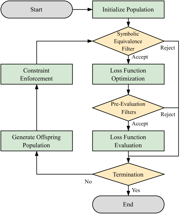
Figure 1: An overview of the EvoMAL framework, showing the pipeline for learning loss functions at meta-training time.

The symbolic search algorithm used in EvoMAL follows a prototypical implementation of GP; as shown in Fig. 1. First, initialization is performed via randomly generating a population of 25 expression trees, where the inner nodes are selected from the function set and the leaf nodes from the terminal set. Subsequently, the main loop begins by performing the loss function optimization and evaluation stages to determine each loss function’s respective fitness, discussed in Sections 3.3 and 3.4, respectively. Following this, a new offspring population of equivalent size is constructed via crossover, mutation, and elitism. For crossover, two loss functions are selected via tournament selection and combined using a one-point crossover with a crossover rate of $70\%$. For mutation, a loss function is selected, and a uniform mutation is applied with a mutation rate of $25\%$. Finally, to ensure performance does not degrade, elitism is used to retain top-performing loss functions with an elitism rate of $5\%$. The main loop is iteratively repeated 50 times, and the loss function with the best fitness is selected as the final learned loss function. Note, to reduce the computational overhead of the meta-learning process, a number of time-saving measures, which we further refer to as filters, have been incorporated into the EvoMAL algorithm. This is discussed in detail in Section 3.5.

3.2.3 Constraint Enforcement

When using GP, the evolved expressions often violate the constraint that a loss function must have as arguments $f_{\theta}(x)$ and $y$. Our preliminary investigation found that often over 50% of the loss functions in the first few generations violated this constraint. Thus far, existing methods for handling this issue have been inadequate; for example, in [28], violating loss functions were assigned the worst-case fitness, such that selection pressure would phase out those loss functions from the population. Unfortunately, this approach degrades search efficiency, as a subset of the population is persistently searching infeasible regions of the search space. To resolve this, we propose a simple but effective corrections strategy to violating loss functions, which randomly selects a terminal node and replaces it with a random binary node, with arguments $f_{\theta}(x)$ and $y$ in no predetermined order.

An additional optional constraint enforceable in the EvoMAL algorithm is that the learned loss function can always return a non-negative output $\mathcal{M}:\mathbb{R}^{2}\rightarrow\mathbb{R}_{0}^{+}$. This is achieved via the loss function’s output being passed through an output activation function $\varphi$, such as the smooth $Softplus(x)=ln(1+e^{x})$ activation. Note that this can be omitted by using an $Identity(x)=x$ activation if we choose not to enforce this constraint.

3.3 Loss Function Optimization

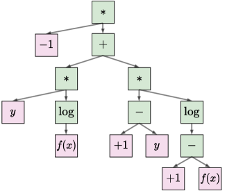
(a)

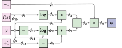
(b)

Figure 2: Overview of the transitional procedure used to covert $\mathcal{M}$ into a trainable meta-loss network $\mathcal{M}_{\phi}^{\mathsf{T}}$.

Numerous empirical results have shown that local-search is imperative when using GP to get state-of-the-art results [56, 28]. Therefore, unrolled differentiation [57, 58, 59, 60], an efficient gradient-based local search approach is integrated into the proposed method. To utilize unrolled differentiation in the EvoMAL framework, we must first transform the expression tree-based representation of $\mathcal{M}$ into a compatible representation. In preparation for this, a transitional procedure takes each loss function $\mathcal{M}$, represented as a GP expression and converts it into a trainable network, as shown in Fig. 2. First, a graph transpose operation $\mathcal{M}^{\mathsf{T}}$ is applied to reverse the edges such that they now go from the terminal (leaf) nodes to the root node. Following this, the edges of $\mathcal{M}^{\mathsf{T}}$ are parameterized by $\phi$, giving $\mathcal{M}_{\phi}^{\mathsf{T}}$, which we further refer to as a meta-loss network to delineate it clearly from its prior state. Finally, to initialize $\mathcal{M}_{\phi}^{\mathsf{T}}$, the weights are sampled from $\phi\sim\mathcal{N}(1,1\mathrm{e}{-3})$, such that $\mathcal{M}_{\phi}^{\mathsf{T}}$ is initialized from its (near) original unit form, where the small amount of variance is to break any network symmetry.

3.3.1 Unrolled Differentiation

In: $\mathcal{M}\leftarrow$ Loss function learned by GP
$\mathcal{S}_{meta}\leftarrow$ Number of meta gradient steps
$\mathcal{S}_{base}\leftarrow$ Number of base gradient steps

$\mathcal{M}_{\phi}^{\mathsf{T}}\leftarrow$ Transpose and parameterize edges of $\mathcal{M}$

$\phi_{0}\leftarrow$ Initialize meta-loss network weights $\mathcal{M}_{\phi}^{\mathsf{T}}$

for $i\in\{0,...,\mathcal{S}_{meta}\}$ do

       for $j\in\{0,...,|\mathcal{D}_{Train}|\}$ do

             $\theta_{0}\leftarrow$ Initialize parameters of base learner

             for $k\in\{0,...,\mathcal{S}_{base}\}$ do

                   $X$, $y$ $\leftarrow$ Sample task $\mathcal{T}_{j}\sim p(\mathcal{T})$

                   $\mathcal{M}_{learned}\leftarrow\mathcal{M}_{\phi}^{\mathsf{T}}(y,f_{\theta}(X))$

                   $\theta_{k+1}\leftarrow\theta_{k}-\alpha\nabla_{\theta}\mathcal{M}_{learned}$

                  

            $\mathcal{L}_{task_{j}}\leftarrow\mathcal{L}_{\mathcal{T}}(y,f_{\theta_{new}}(X))$

            

      $\phi_{i+1}\leftarrow\phi_{i}-\eta\nabla_{\phi}\sum_{j}\mathcal{L}_{task_{j}}$

      

Algorithm 1 Loss Function Optimization

For simplicity, we constrain the description of loss function optimization to the vanilla backpropagation case where the meta-training set $\mathcal{D}_{Train}$ contains one task, i.e. $|\mathcal{D}_{Train}|=1$; however, the full process where $|\mathcal{D}_{Train}|>1$ is given in Algorithm 1.

To learn the weights $\phi$ of the meta-loss network $\mathcal{M}_{\phi}^{\mathsf{T}}$ at meta-training time with respect to base learner $f_{\theta}(x)$, we first use the initial values of $\phi$ to produce a base loss value $\mathcal{M}_{learned}$ based on the forward pass of $f_{\theta}(x)$.

$$\mathcal{M}_{learned}=\mathcal{M}_{\phi}^{\mathsf{T}}(y,f_{\theta}(x))$$ (4)

Using $\mathcal{M}_{learned}$, the weights $\theta$ are optimized by taking a predetermined number of inner base gradient steps $\mathcal{S}_{base}$, where at each step a new batch is sampled and a new base loss value is computed. Similar to the findings in [24], we find $\mathcal{S}_{base}=1$ is usually sufficient to obtain good results. Each step is computed by taking the gradient of the loss value with respect to $\theta$, where $\alpha$ is the base learning rate.

$$\begin{split}\theta_{new}&=\theta-\alpha\nabla_{\theta}\mathcal{M}_{\phi}^{\mathsf{T}}(y,f_{\theta}(x))\\ &=\theta-\alpha\nabla_{\theta}\mathbb{E}_{{X},y}\big{[}\mathcal{M}_{\phi}^{\mathsf{T}}(y,f_{\theta}(x))\big{]}\end{split}$$ (5)

where the gradient computation can be decomposed via the chain rule into the gradient of $\mathcal{M}_{\phi}^{\mathsf{T}}$ with respect to the product of the base learner predictions $f_{\theta}(x)$ and the gradient of $f$ with parameters $\theta$.

$$\theta_{new}=\theta-\alpha\nabla_{f}\mathcal{M}_{\phi}^{\mathsf{T}}(y,f_{\theta}(x))\nabla_{\theta}f_{\theta}(x)$$ (6)

Following this, $\theta$ has been updated to $\theta_{new}$ based on the current meta-loss network weights; $\phi$ now needs to be updated to $\phi_{new}$ based on how much learning progress has been made. Using the new base learner weights $\theta_{new}$ as a function of $\phi$, we utilize the concept of a task loss $\mathcal{L}_{\mathcal{T}}$ to produce a meta loss value $\mathcal{L}_{task}$ to optimize $\phi$ through $\theta_{new}$.

$$\mathcal{L}_{task}=\mathcal{L}_{\mathcal{T}}(y,f_{\theta_{new}}(x))$$ (7)

where $\mathcal{L}_{\mathcal{T}}$ is selected based on the respective application — for example, the mean squared error loss for the task of regression or the categorical cross-entropy loss for multi-class classification. Optimization of the meta-loss network loss weights $\phi$ now occurs by taking the gradient of $\mathcal{L}_{\mathcal{T}}$ with respect to $\phi$, where $\eta$ is the meta learning rate.

$$\begin{split}\phi_{new}&=\phi-\eta\nabla_{\phi}\mathcal{L}_{\mathcal{T}}(y,f_{\theta_{new}}(x))\\ &=\phi-\eta\nabla_{\phi}\mathbb{E}_{{X},y}\big{[}\mathcal{L}_{\mathcal{T}}(y,f_{\theta_{new}}(x))\big{]}\end{split}$$ (8)

where the gradient computation can be decomposed by applying the chain rule as shown in Equation (9) where the gradient with respect to the meta-loss network weights $\phi$ requires the new model parameters $\theta_{new}$.

$$\phi_{new}=\phi-\eta\nabla_{f}\mathcal{L}_{\mathcal{T}}\nabla_{\theta_{new}}f_{\theta_{new}}\nabla_{\phi}\theta_{new}$$ (9)

This process is repeated for a predetermined number of meta gradient steps $S_{meta}=250$, which was selected via cross-validation. Following each meta gradient step, the base learner weights $\theta$ is reset. Note that Equations (5)–(6) and (8)–(9) can alternatively be performed via automatic differentiation.

3.4 Loss Function Evaluation

Figure 3: Overview of the EvoMAL algorithm at meta-testing time, where the base network $f_{\theta}(x)$, shown (left) as the popular LeNet-5 architecture, is trained using the meta-loss network $\mathcal{M}_{\phi}^{\mathsf{T}}$ (right) found at meta-training time as the loss function.

To derive the fitness $\mathcal{F}$ of $\mathcal{M}_{\phi}^{\mathsf{T}}$, a conventional training procedure is used as summarized in Algorithm 2, where $\mathcal{M}_{\phi}^{\mathsf{T}}$ is used in place of a traditional loss function to train $f_{\theta}(x)$ over a predetermined number of base gradient steps $S_{testing}$. This training process is identical to training at meta-testing time as shown in Fig. 3. The final inference performance of $\mathcal{M}_{\phi}^{\mathsf{T}}$ is assigned to $\mathcal{F}$, where any differentiable or non-differentiable performance metric $\mathcal{L}_{\mathcal{P}}$ can be used. For our experiments we use the error rate to compute $\mathcal{F}$.

In: $\mathcal{M}_{\phi}^{\mathsf{T}}\leftarrow$ Loss function learned by EvoMAL
$S_{testing}\leftarrow$ Number of base testing gradient steps

for $i\in\{0,...,|\mathcal{D}|\}$ do

       $\theta_{i}\leftarrow$ Initialize parameters of base learner $f_{\theta_{i}}$

       $X_{i}$, $y_{i}$ $\leftarrow$ Sample task $\mathcal{T}_{i}\sim p(\mathcal{T})$

       for $j\in\{0,...,S_{testing}\}$ do

             $\mathcal{L}_{learned}\leftarrow\mathcal{M}_{\phi}^{\mathsf{T}}(y_{i},f_{\theta_{i}}(X_{i}))$

             $\theta_{i}\leftarrow\theta_{i}-\alpha\nabla_{\theta_{i}}\mathcal{L}_{learned}$

            

$\mathcal{F}\leftarrow\frac{1}{|\mathcal{D}|}\sum_{i}\mathcal{L}_{\mathcal{P}}(y_{i},f_{\theta_{i}}(X_{i}))$

Algorithm 2 Loss Function Evaluation

3.5 Time Saving Measures (Filters)

Optimizing and evaluating a large number of candidate loss functions can become prohibitively expensive. Fortunately, in the case of loss function learning, a number of techniques can be employed to reduce significantly the computational overhead of the otherwise very costly meta-learning process.

3.5.1 Symbolic Equivalence Filter

For the GP-based symbolic search, a loss archival strategy based on a key-value pair structure with $\Theta(1)$ lookup is used to ensure that symbolically equivalent loss functions are not reevaluated. Two expression trees are said to be symbolically equivalent when they contain identical operations (nodes) in an identical configuration [61, 62, 63]. Loss functions that are identified by the symbolic equivalence filter skip both the loss function optimization and evaluation stage and are placed directly in the offspring population with their fitness cached.

3.5.2 Pre-Evaluation Filter - Poor Training Dynamics

Following loss function optimization, the candidate solution’s fitnesses are evaluated. This costly fitness evaluation can be obviated in many cases since many of the loss functions found, especially in the early generations, are non-convergent and produce poor training dynamics. We use the loss rejection protocol employed in [30] as a filter to identify candidate loss functions that should skip evaluation and be assigned the worst-case fitness automatically.

The loss rejection protocol takes a batch of $B$ randomly sampled instances from $\mathcal{D}_{Train}$ and using an untrained network $f_{\theta_{0}}(x)$ produces a set of predictions and their corresponding true target values $\{(\hat{y_{b}},y_{b})\}_{b=1}^{B}$. As minimizing the proper loss function $\mathcal{M}_{\phi}^{\mathsf{T}}$ should correspond closely with optimizing the performance metric $\mathcal{L}_{\mathcal{P}}$, a correlation $g$ between $\mathcal{M}_{\phi}^{\mathsf{T}}$ and $\mathcal{L}_{\mathcal{P}}$ can be calculated.

$$g(\mathcal{M}_{\phi}^{\mathsf{T}})=\sum_{b=1}^{B}\Big{[}\mathcal{L}_{\mathcal{P}}(\hat{y_{b}},y_{b})-\mathcal{L}_{\mathcal{P}}(\hat{y_{b}^{*}}(\mathcal{M}_{\phi}^{\mathsf{T}}),y_{b})\Big{]},$$ (10)

where $\hat{y_{b}^{*}}$ is the network predictions optimized with the candidate loss function $\mathcal{M}_{\phi}^{\mathsf{T}}$. Importantly, optimization is performed directly to $\hat{y_{b}^{*}}$, as opposed to the network parameters $\theta$, thus omitting any base network computation (i.e. no training of the base network).

$$\hat{y_{b}^{*}}(\mathcal{M}_{\phi}^{\mathsf{T}})=\arg\min_{\hat{y_{b}^{*}}}\mathcal{M}_{\phi}^{\mathsf{T}}(\hat{y_{b}^{*}},y_{b})$$ (11)

A large positive correlation indicates that minimizing $\mathcal{M}_{\phi}^{\mathsf{T}}$ corresponds to minimizing the given performance metric $\mathcal{L}_{\mathcal{P}}$ (assuming both $\mathcal{M}_{\phi}^{\mathsf{T}}$ and $\mathcal{L}_{\mathcal{P}}$ are for minimization). In contrast to this, if $g\leq 0$, then $\mathcal{M}_{\phi}^{\mathsf{T}}$ is regarded as being unpromising and should be assigned the worst-case fitness and not evaluated. The underlying assumption here is that if a loss function cannot directly optimize the labels, it is unlikely to be able to optimize the labels through the model weights $\theta$ successfully.

3.5.3 Pre-Evaluation Filter - Gradient Equivalence

Many of the candidate loss functions found in the later generations, as convergence is approached, have near-identical gradient behavior (i.e. functionally equivalence). To address this, the gradient equivalence checking strategy from [30] is employed as another filter to identify loss functions that have near-identical behavior to those seen previously. Using the prediction from previously, the gradient norms are computed.

$$\{\parallel\nabla_{\hat{y}_{b}}\mathcal{M}_{\phi}^{\mathsf{T}}\parallel_{2}\}_{b=1}^{B}$$ (12)

If, for all of the $B$ samples, two-loss functions have the same gradient norms within two significant digits, they are considered functionally equivalent, and their fitness is cached.

3.5.4 Partial Training Sessions

For the remaining loss functions whose fitness evaluation cannot be fully obviated, we compute the fitness $\mathcal{F}$ using a truncated number of gradient steps $\mathcal{S}_{testing}=500$. As noted in [64, 65], performance at the beginning of training is correlated with the performance at the end of training; consequently, we can obtain an estimate of what $\mathcal{F}$ would be by performing a partial training session of the base model. Preliminary experiments with EvoMAL showed minimal short-horizon bias [66], and the ablation study found in [25] indicated that $500$ gradient steps during loss function evaluation is a good trade-off between final base-inference performance and meta-training time. In addition to significantly reducing the run-time of EvoMAL, reducing the value of $\mathcal{S}_{testing}$ has the effect of implicitly optimizing for the base-training convergence and sample-efficiency, as mentioned in [3].

4 Experimental Setup

In this section, the performance of EvoMAL is evaluated. A wide range of experiments are conducted across four datasets and numerous popular network architectures, with the performance contrasted against a representative set of benchmark methods implemented in DEAP [67], PyTorch [68] and Higher [33].

4.1 Benchmark Methods

TABLE II: Classification results reporting the mean $\pm$ standard deviation final inference error rate across 5 independent executions of each algorithm on each task + model pair. Loss functions are directly meta-learned and applied to the same respective task.

Task and Model	Baseline	ML3	TaylorGLO	GP-LFL	EvoMAL (Ours)
MNIST
Logistic 1	0.0787$\pm$0.0009	0.0768$\pm$0.0061	0.0725$\pm$0.0013	0.0781$\pm$0.0052	0.0721$\pm$0.0017
MLP 2	0.0247$\pm$0.0005	0.0201$\pm$0.0081	0.0151$\pm$0.0013	0.0156$\pm$0.0012	0.0152$\pm$0.0012
LeNet-5 3	0.0203$\pm$0.0025	0.0135$\pm$0.0039	0.0137$\pm$0.0038	0.0115$\pm$0.0015	0.0100$\pm$0.0010
CIFAR-10
AlexNet 4	0.1544$\pm$0.0012	0.1450$\pm$0.0028	0.1499$\pm$0.0075	0.1506$\pm$0.0047	0.1437$\pm$0.0033
VGG-16 5	0.0771$\pm$0.0023	0.0700$\pm$0.0006	0.0700$\pm$0.0022	0.0686$\pm$0.0014	0.0687$\pm$0.0016
AllCNN-C 6	0.0761$\pm$0.0015	0.0712$\pm$0.0043	0.0735$\pm$0.0030	0.0701$\pm$0.0022	0.0697$\pm$0.0010
ResNet-18 7	0.0658$\pm$0.0019	0.0584$\pm$0.0022	0.0546$\pm$0.0033	0.0818$\pm$0.0391	0.0528$\pm$0.0015
PreResNet 8	0.0661$\pm$0.0015	0.0660$\pm$0.0016	0.0660$\pm$0.0027	0.0658$\pm$0.0023	0.0655$\pm$0.0018
WideResNet 9	0.0548$\pm$0.0016	0.0549$\pm$0.0040	0.0493$\pm$0.0023	0.0489$\pm$0.0014	0.0484$\pm$0.0018
SqueezeNet 10	0.0838$\pm$0.0013	0.0800$\pm$0.0012	0.0800$\pm$0.0025	0.0810$\pm$0.0016	0.0796$\pm$0.0017
CIFAR-100
WideResNet 9	0.2293$\pm$0.0017	0.2299$\pm$0.0027	0.2347$\pm$0.0077	0.3382$\pm$0.1406	0.2276$\pm$0.0033
PyramidNet 11	0.2527$\pm$0.0028	0.2792$\pm$0.0226	0.3064$\pm$0.0549	0.2747$\pm$0.0087	0.2664$\pm$0.0063
SVHN
WideResNet 9	0.0340$\pm$0.0005	0.0335$\pm$0.0003	0.0343$\pm$0.0016	0.0340$\pm$0.0015	0.0329$\pm$0.0013

• Network architecture references:

• McCullagh et al. (2019)

• Baydin et al. (2018)

• LeCun et al. (1998)

• Krizhevsky et al. (2012)

• Simonyan and Zisserman (2015)

• Springenberg et al. (2015)

• He et al. (2015)

• He et al. (2016)

• Zagoruyko and Komodakis (2016)

• N. Iandola et al. (2016)

• Han et al. (2017)

The selection of benchmark methods is intended to showcase the performance of the newly proposed algorithm against the current state-of-the-art. Additionally, the selected methods enable direct comparison between EvoMAL and its derivative methods, which aids in validating the effectiveness of hybridizing the approaches into one unified framework.

• Baseline – Directly using $\mathcal{L}_{\mathcal{T}}$ as the loss function, i.e. using the squared error loss (regression) or cross-entropy loss (classification) and a prototypical training loop (i.e. no meta-learning).

• ML³ Supervised – Gradient-based method proposed in [24], which uses a parametric loss function defined by a two hidden layer feed-forward network trained with generalized inner loop meta-learning, i.e. the method shown in Section 3.3.

• TaylorGLO — Evolution-based method proposed by [25], which uses a third-order Taylor-polynomial representation for the meta-learned loss functions, optimized via covariance matrix adaptation evolution strategy.

• GP-LFL – A proxy method used to aggregate previous GP-based approaches for loss function learning without any local-search mechanisms, using an identical setup to EvoMAL excluding Section 3.3.

Where possible, hyper-parameter selection has been standardized across the benchmark methods to allow for a fair comparison. For example, in TaylorGLO, GP-LFL, and EvoMAL we use an identical population size $=25$ and number of generations = $50$. For unique hyper-parameters, the suggested values from the respective publications are utilized.

4.2 Benchmark Problems

Regarding the problem domains, seven datasets have been selected. Three tabulated regression tasks are initially used: Diabetes, Boston Housing, and California Housing, all taken from the UCI’s dataset repository [69]. Following this, analogous to the prior literature [28, 25, 24], both MNIST [70] and CIFAR-10 [71] are employed to evaluate the benchmark methods. Finally, experiments are conducted on the more challenging but related domains of SVHN [72] and CIFAR-100 [71], respectively.

For the three tabulated regression tasks, the datasets are partitioned 60:20:20 for training, validation, and testing. Furthermore, to improve the training dynamics, both the features and labels are normalized. For the remaining datasets, the original training-testing partitioning is used, with 10% of the training instances allocated for validation. In addition, data augmentation techniques consisting of normalization, random horizontal flips, and cropping are applied to the training data during meta and base training.

Regarding the base models, a diverse set of neural network architectures are utilized to evaluate the selected benchmark methods. For Diabetes, Boston Housing, and California Housing, a simple Multi-Layer Perceptron (MLP) taken from [73] with 1000 hidden nodes and ReLU activations are employed. For MNIST, Logistic Regression [74], MLP, and the well-known LeNet-5 architecture [70] are used. While on CIFAR-10 AlexNet [75], VGG-16 [76], AllCNN-C [77], ResNet-18 [78], Preactivation ResNet-101 [79], WideResNet 28-10 [80] and SqueezeNet [81] are used. For the remaining datasets, WideResNet 28-10 is again used, as well as PyramidNet [82] on CIFAR-100. All models are trained using stochastic gradient descent (SGD) with momentum. The model hyper-parameters are selected using their respective values from the literature in an identical setup to [25, 24].

Finally, due to the stochastic nature of the benchmark methods, we perform five independent executions of each method on each dataset + model pair. Furthermore, we control for the base initializations such that each method gets identical initial conditions across the same random seed; thus, any difference in variance between the methods can be attributed to the respective algorithms.

TABLE III: Regression results reporting the mean $\pm$ standard deviation final inference testing mean squared error across 5 executions of each algorithm on each task + model pair. Loss functions are directly meta-learned and applied to the same respective task.

Task and Model	Baseline	ML3	TaylorGLO	GP-LFL	EvoMAL (Ours)
Diabetes
MLP 1	0.3829$\pm$0.0065	0.4278$\pm$0.1080	0.3620$\pm$0.0096	0.3746$\pm$0.0577	0.3573$\pm$0.0198
Boston
MLP 1	0.1304$\pm$0.0057	0.2474$\pm$0.0526	0.1349$\pm$0.0074	0.1341$\pm$0.0082	0.1314$\pm$0.0131
California
MLP 1	0.2326$\pm$0.0019	0.2438$\pm$0.0189	0.1794$\pm$0.0156	0.2071$\pm$0.0609	0.1723$\pm$0.0048

• Network architecture references:

• Baydin et al. (2018)

TABLE IV: Loss function transfer results reporting the mean $\pm$ standard deviation final inference testing mean squared error
(regression) or error rate (classification) across 5 independent executions of each algorithm on each task + model pair. Loss
functions are meta-learned on CIFAR-10 with the respective model, and then transferred to CIFAR-100 using that same model.

Task and Model	Baseline	ML3	TaylorGLO	GP-LFL	EvoMAL (Ours)
CIFAR-100
AlexNet 1	0.5262$\pm$0.0094	0.7735$\pm$0.0295	0.5543$\pm$0.0138	0.5329$\pm$0.0037	0.5324$\pm$0.0031
VGG-16 2	0.3025$\pm$0.0022	0.3171$\pm$0.0019	0.3155$\pm$0.0021	0.3171$\pm$0.0041	0.3115$\pm$0.0038
AllCNN-C 3	0.2830$\pm$0.0021	0.2817$\pm$0.0032	0.4191$\pm$0.0058	0.2849$\pm$0.0012	0.2807$\pm$0.0028
ResNet-18 4	0.2474$\pm$0.0018	0.6000$\pm$0.0173	0.2436$\pm$0.0032	0.2373$\pm$0.0013	0.2326$\pm$0.0014
PreResNet 5	0.2908$\pm$0.0065	0.2838$\pm$0.0019	0.2993$\pm$0.0030	0.2839$\pm$0.0025	0.2899$\pm$0.0024
WideResNet 6	0.2293$\pm$0.0017	0.2448$\pm$0.0063	0.2285$\pm$0.0031	0.2276$\pm$0.0028	0.2238$\pm$0.0017
SqueezeNet 7	0.3178$\pm$0.0015	0.3402$\pm$0.0057	0.3178$\pm$0.0012	0.3343$\pm$0.0054	0.3166$\pm$0.0026

• Network architecture references:

• Krizhevsky et al. (2012)

• Simonyan and Zisserman (2015)

• Springenberg et al. (2015)

• He et al. (2015)

• He et al. (2016)

• Zagoruyko and Komodakis (2016)

• N. Iandola et al. (2016)

5 Results and Analysis

The results and analysis are approached from three distinct angles. First, the experimental results reporting the final inference meta-testing performance when using meta-learned loss functions for base-training are presented in Section 5.1. Following this, the performance of the loss function learning algorithms themselves at meta-training time is compared in Section 5.2. The focus is turned towards an analysis of the meta-learned loss functions themselves to highlight some of the loss functions developed by EvoMAL on both classification and regression tasks in Section 5.3. Finally, an analysis is given in Sections 5.4 and 5.5, which explore two of the central hypotheses for why meta-learned loss functions are so performant compared to their handcrafted counterparts.

5.1 Meta-Testing Performance

A summary of the final inference testing results reporting the average error rate (classification) or mean squared error (regression) across the seven tested datasets is shown in Tables II and III respectively, where the same dataset and model pair are used for both meta-training and meta-testing. The results show that meta-learned loss functions consistently produce superior performance compared to the baseline handcrafted squared error loss and cross-entropy loss. Large performance gains are made on the California Housing, MNIST, and CIFAR-10 datasets, while more modest gains are observed on Diabetes, WideResNet CIFAR-100 and SVHN, and worse performance on Boston Housing MLP and CIFAR-100 PyramidNet, a similar finding to that found in [25].

Contrasting the performance of EvoMAL to the benchmark loss function learning methods, it is shown that EvoMAL consistently meta-learns more performant loss functions, with better performance on all task + model pairs except for on CIFAR-10 VGG-16, where performance is comparable to the next best method. Furthermore, compared to its derivative methods ML³ and GP-LFL, EvoMAL successfully meta-learns loss functions on more complex tasks, i.e. CIFAR-100 and SVHN, whereas the other techniques often struggle to improve upon the baseline. These results empirically confirm the benefits of unifying existing approaches to loss function learning into one unified framework. Furthermore, the results clearly show the necessity for integrating local-search techniques in GP-based loss function learning.

In general, it is observed that smaller performance gains across all methods are made when using meta-learned loss functions relative to prior research into loss function learning. For example, prior research has reported increasing the accuracy of a classification model by up to 5% in some cases when using meta-learned loss functions compared to the baseline cross-entropy loss. However, with heavily tuned baselines, optimizing for both the learning rate and the number of gradient steps, such performance gains were not obtainable. This suggests that a proportion of the performance gains reported previously by loss function learning methods likely comes from an implicit tuning effect on the training dynamics as opposed to a direct effect from using a different loss function. Implicit tuning is not a drawback of loss function learning as a paradigm; however, it is essential to disentangle the effects. In Section 5.3, further experiments are given to isolate the effects.

5.1.1 Loss Function Transfer

(a) Diabetes
MLP

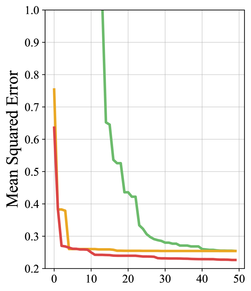
(b) Boston
MLP

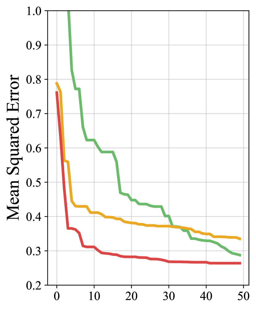
(c) California
MLP

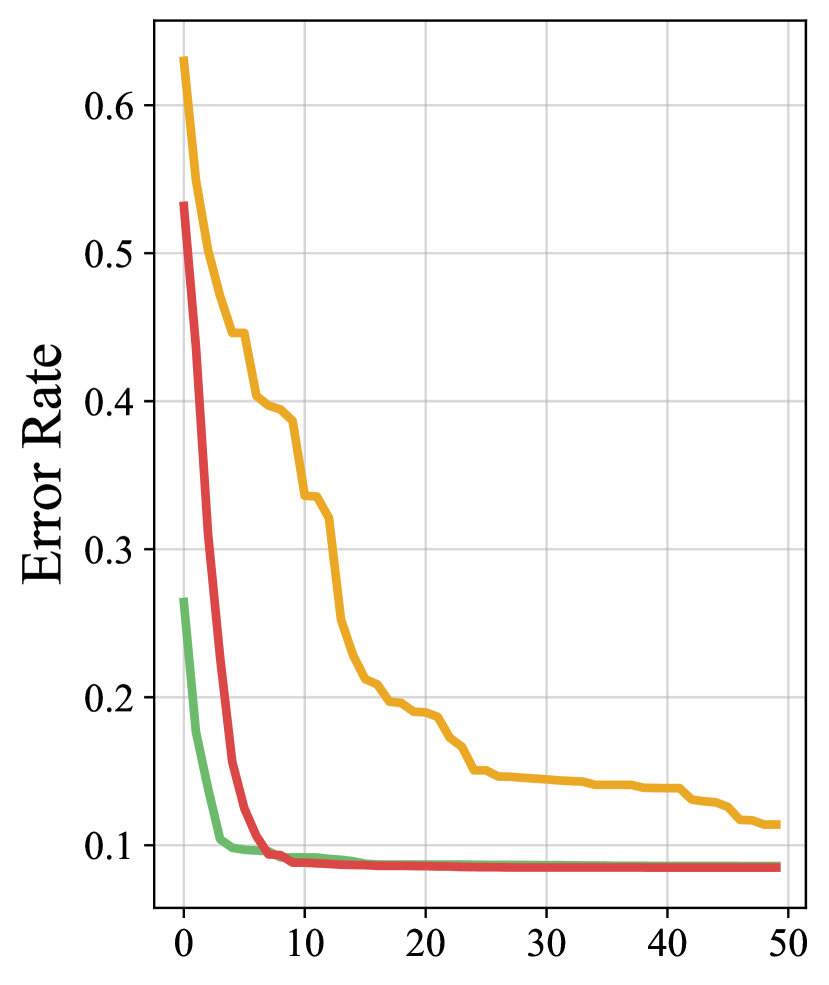
(d) MNIST
Logistic

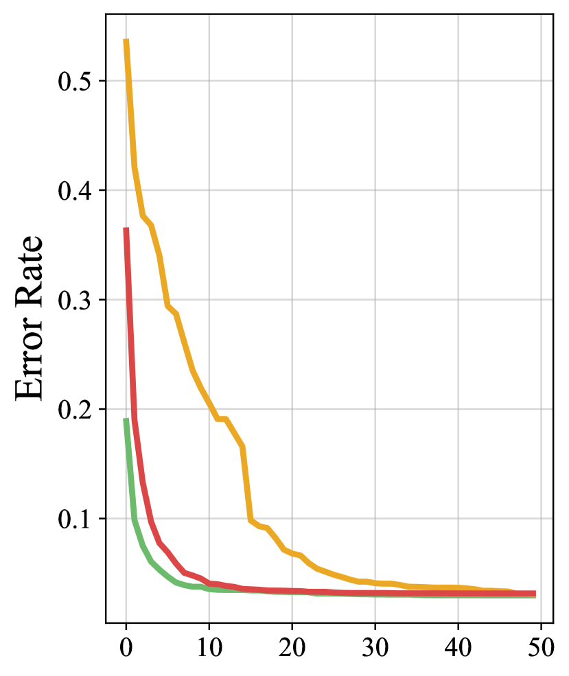
(e) MNIST
MLP

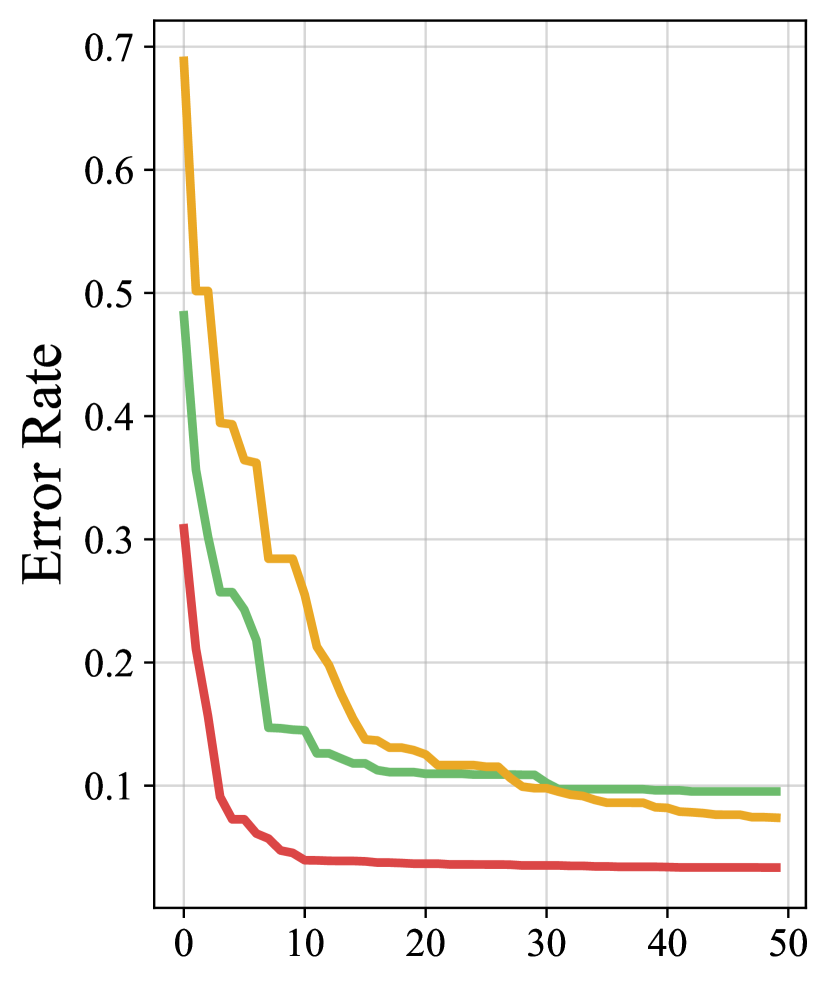
(f) MNIST
LeNet-5

(g) CIFAR-10
AlexNet

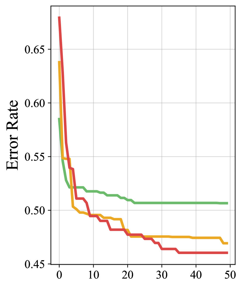
(h) CIFAR-10
VGG-16

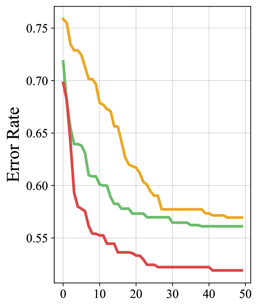
(i) CIFAR-10
AllCNN-C

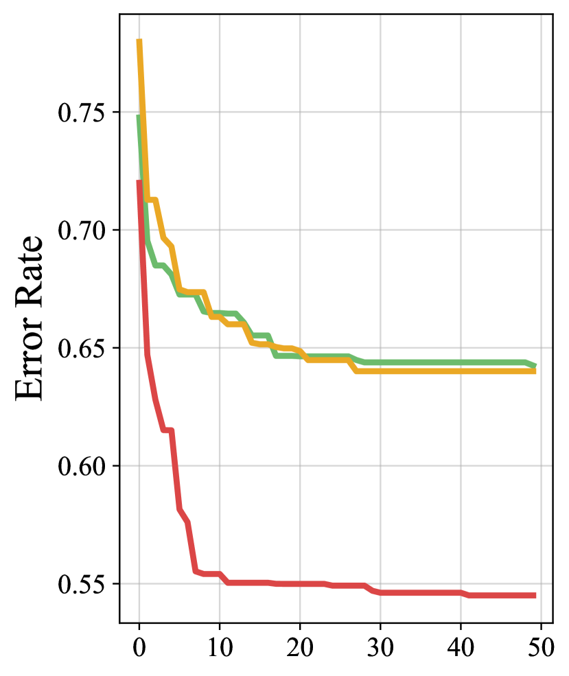
(j) CIFAR-10
ResNet-18

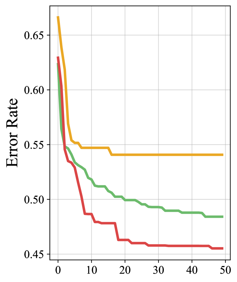
(k) CIFAR-10
WideResNet 28-10

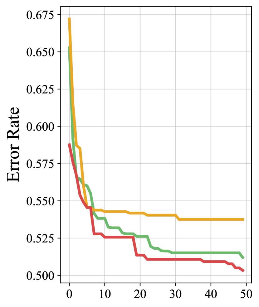
(l) CIFAR-10
SqueezeNet

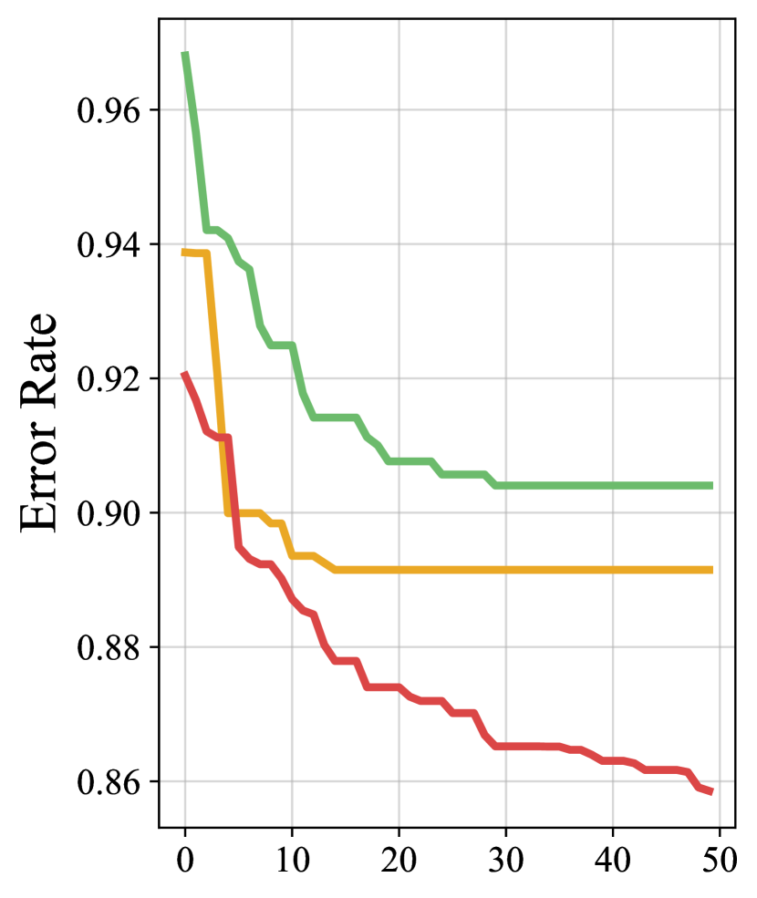
(m) CIFAR-100
WideResNet 28-10

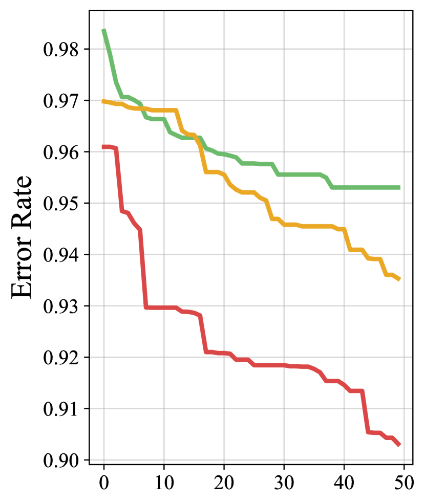
(n) CIFAR-100
PyramidNet

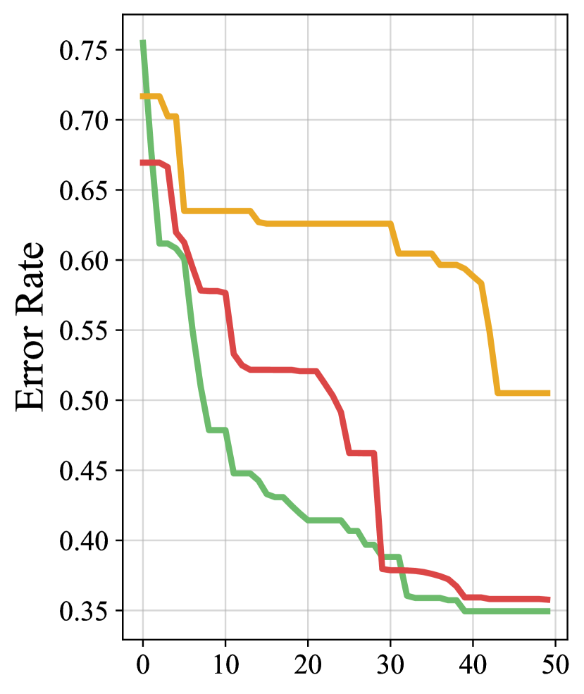
(o) SVHN
WideResNet 28-10

Figure 4: Mean meta-training learning curves across 5 independent executions of each algorithm, showing the fitness score (y-axis) against generations (x-axis), where a generation is equivalent to 25 evaluations. Best viewed in color.

To further validate the performance of EvoMAL, the much more challenging task of loss function transfer is assessed, where the meta-learned loss functions learned in one source domain are transferred to a new but related target domain. In our experiments, the meta-learned loss functions are taken directly from CIFAR-10 (in the previous section) and then transferred to CIFAR-100 with no further computational overhead, using the same model as the source. To ensure a fair comparison is made to the baseline, only the best-performing loss function found across the 5 random seeds from each method on each task + model pair are used. A summary of the final inference testing error rates when performing loss function transfer is given in Table IV.

The results show that even when using a single-task meta-learning setup where cross-task generalization is not explicitly optimized for, meta-learned loss functions can still be transferred with some success. In regards to meta-generalization, it is observed that EvoMAL and GP-LFL transfer their relative performance the most consistently to new tasks. In contrast, ML³, which uses a neural network-based representation, often fails to generalize to the new tasks, a finding similar to [3] which found that symbolic representations often generalize better than sub-symbolic representations. Another notable result is that on both AlexNet and VGG-16 in the direct meta-learning setup, large gains in performance compared to the baseline are observed, as shown in Table II. Conversely, when the learned loss functions are transferred to CIFAR-100, all the loss function learning methods perform worse than the baseline as shown in Table IV. These results suggest that the learned loss functions have likely been meta-overfitted to the source task and that meta-regularization is an important aspect to consider for loss function transfer.

5.2 Meta-Training Performance

The meta-training learning curves are given in Fig. 4, where the search performance of EvoMAL is compared to TaylorGLO and GP-LFL at each iteration and the performance is quantified by the fitness function using partial training sessions. Based on the results, it is very evident that adding local-search mechanisms into the EvoMAL framework dramatically increases the search effectiveness of GP-based loss function learning techniques. EvoMAL is observed to consistently attain much better performance than GP-LFL in a significantly shorter number of iterations. In almost all tasks, EvoMAL is shown to find better performing loss functions in the first 5 to 10 generations compared to those found by GP-LFL after 50.

Contrasting EvoMAL to TaylorGLO, it is generally shown again that for most tasks, EvoMAL produces better solutions in a smaller number of iterations. Furthermore, performance does not appear to prematurely converge on the more challenging tasks of CIFAR-100 and SVHN compared to TaylorGLO and GP-LFL. Interestingly, on both CIFAR-10 AlexNet and SVHN WideResNet, TaylorGLO is able to achieve slightly better final solutions compared to EvoMAL on average; however, as shown by the final inference testing error rates in Tables II and III, these don’t necessarily correspond to better final inference performance. This discrepancy between meta-training curves and final inference is also observed in the inverse case, where EvoMAL is shown to have much better learning curves than both TaylorGLO and GP-LFL, e.g. in CIFAR-10 AllCNN-C and ResNet-18. However, the final inference error rates of EvoMAL in Table II are only marginally better than those of TaylorGLO and GP-LFL.

This phenomenon is likely due to some of the meta-learned loss functions implicitly tuning the learning rate (discussed further in 5.3). Implicit learning rate tuning can result in increased convergence capabilities, i.e., faster learning which results in better fitness when using partial training sessions, but does not necessarily imply a strongly generalizing and robustly trained model at meta-testing time when using full training sessions.

5.2.1 Meta-Training Run-Time

TABLE V: Average run-time of the meta-training process for each of the benchmark methods. Each algorithm is run on a single Nvidia RTX A5000, and the results are reported in hours.

Task and Model	ML3	TaylorGLO	GP-LFL	EvoMAL
Diabetes
MLP	0.01	0.83	0.53	1.93
Boston
MLP	0.01	0.85	0.46	1.59
California
MLP	0.01	0.94	0.84	2.06
MNIST
Logistic	0.02	1.44	0.61	2.45
MLP	0.03	2.06	0.77	5.31
LeNet-5	0.03	2.30	0.82	3.29
CIFAR-10
AlexNet	0.03	3.75	1.04	5.90
VGG-16	0.12	4.67	0.89	9.12
AllCNN-C	0.12	4.55	0.90	8.77
ResNet-18	0.60	9.14	1.02	54.22
PreResNet	0.41	8.40	0.96	41.73
WideResNet	0.63	12.85	0.98	66.72
SqueezeNet	0.12	4.95	0.41	11.18
CIFAR-100
WideResNet	0.20	20.34	1.34	57.61
PyramidNet	0.20	24.83	1.32	49.89
SVHN
WideResNet	0.20	41.57	1.09	67.28

The use of a two-stage discovery process by EvoMAL enables the development of highly effective loss functions, as shown by the meta-training and meta-testing results. Producing on average models with superior inference performance compared to TaylorGLO and ML³ which only optimize the coefficients/weights of fixed parametric structures, and GP-LFL which uses no local-search techniques. However, this bi-level optimization procedure where both the model structure and parameters are inferred adversely affects the computational efficiency of the meta-learning process, as shown in Table V, which reports the average run-time (in hours) of meta-training for each loss function learning method.

The results show that EvoMAL is more computationally expensive than ML³ and GP-LFL and approximately twice as expensive as TaylorGLO on average. Although EvoMAL is computationally expensive, it should be emphasized that this is still dramatically more efficient than GLO [28], the bi-level predecessor to TaylorGLO, whose costly meta-learning procedure required a supercomputer for even very simple datasets such as MNIST.

The bi-level optimization process of EvoMAL is made computationally tractable by replacing the costly CMA-ES loss optimization stage from GLO with a significantly more efficient gradient-based procedure. On CIFAR-10, using the relatively small network, PreResNet-20 GLO required 11,120 partial training sessions and approximately 171 GPU days of computation [28, 25] compared to EvoMAL, which only needed on average 1.7 GPU days. In addition, the reduced run times of EvoMAL can also be partially attributed to the application of time-saving filters, which enables a subset of the loss optimizations and fitness evaluations to be either cached or obviated entirely.

To summarize the effects of the time-saving filters, a set of histograms are presented in Fig. 5 showing the frequency of occurrence throughout the evolutionary process. Examining the symbolic equivalence filter results, it is observed that, on average, $\sim$10% of the loss functions are identified as being symbolically equivalent at each generation; consequently, these loss functions have their fitness cached, and $\sim$90% of the loss functions progress to the next stage and are optimized. Regarding the pre-evaluation filters, the rejection protocol initially rejects the majority of the optimized loss functions early in the search for being unpromising, automatically assigning them the worst-case fitness. In contrast, in the late stages of the symbolic search, this filter occurs incrementally less frequently, suggesting that convergence is being approached, further supported by the frequency of occurrence of the gradient equivalence filter, which caches few loss functions at the start of the search, but many near the end. Due to this aggressive filtering, only $\sim$25% of the population at each generation have their fitness evaluated, which helps to reduce the run-time further.

Note that the run-time of EvoMAL can be further reduced for large-scale optimization problems through parallelization to distribute loss function optimization and evaluation across multiple GPUs or clusters.

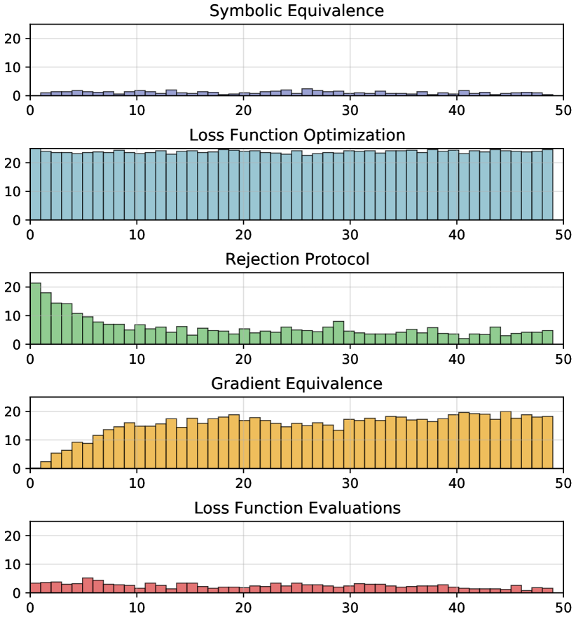
Figure 5: Frequencies of occurrence of the time saving filters, and the corresponding frequencies of loss optimization and evaluation throughout the symbolic search process. Reporting the average frequencies across all task + model pairs and independent executions of EvoMAL.

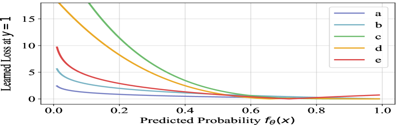
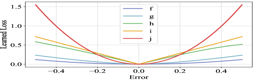
Figure 6: Example loss functions meta-learned by EvoMAL. The left plot shows classification loss functions, and right shows regression loss functions. Best viewed in color.

5.3 Meta-Learned Loss Functions

TABLE VI: Example loss functions meta-learned by EvoMAL, where solutions have been numerically and algebraically simplified. Furthermore, the parameters $\phi$ have also been omitted for improved clarity and parsimony.

a.	$|\log(\sqrt{y\cdot f_{\theta}(x)}+\epsilon)|$
b.	$\log(y\cdot f_{\theta}(x))+\sqrt{\log(y\cdot f_{\theta}(x))}^{2}$
c.	$((y-f_{\theta}(x))/f_{\theta}(x))^{4}$
d.	$y^{3}+f_{\theta}(x)^{3}+f_{\theta}(x)\cdot y^{2}+f_{\theta}(x)^{2}\cdot y$
e.	$|\log((y\cdot f_{\theta}(x))^{2}+\epsilon)|$
f.	$(f_{\theta}(x)-\min(\max(y,-1),1))^{2}$
g.	$|y\cdot(\sqrt{|y/\sqrt{1+f_{\theta}(x)^{2}}|})|$
h.	$|(y/(1+\log(|y-1|)^{2}))-f_{\theta}(x)|$
i.	$\sqrt{|y\cdot(y-f_{\theta}(x))|}$
j.	$\sqrt{|y-f_{\theta}(x)|}$

To better understand why the meta-learned loss functions produced by EvoMAL are so performant, an analysis is conducted on a subset of the interesting loss functions found throughout the experiments. In Fig. 6, examples of the meta-learned loss functions produced by EvoMAL are presented. The corresponding loss functions are also given symbolically in Table VI.

5.3.1 Learned Loss Functions for Classification Tasks

The classification loss functions meta-learned by EvoMAL appear to converge upon three classes of loss functions. First are cross-entropy loss variants such as loss functions a) and b), which closely resemble the cross-entropy loss functionally and symbolically. Second, are loss functions that have similar characteristics to the parametric focal loss [83], such as loss functions c) and d). These loss functions recalibrate how easy and hard samples are prioritized; in most cases, very little or no loss is attributed to high-confidence correct predictions, while significant loss is attributed to high-confidence wrong predictions. Finally, loss functions such as e) which demonstrate unintuitive behavior, such as assigning more loss to confident and correct solutions relative to unconfident and correct solutions, a characteristic which induces implicit label smoothing regularization [84, 85], see analysis in Appendix A.

5.3.2 Learned Loss Functions for Regression Tasks

Analyzing the regression loss functions it is observed that there are several unique behaviors particularly around incorporating strategies for improving robustness to outliers. For example in f) the loss function takes on the form of the squared loss; however, it incorporates a thresholding operation via the $\max$ operator for directly limiting the size of the ground truth label. Alternatively in loss functions g), i), and j), there is frequent use of the square root operator, which decreases the loss attributed to increasingly large errors. Finally, we observe that many of the learned loss functions, take on shapes similar to well-known handcrafted loss functions; for example, h) appears to be a cross between the absolute loss and the Cauchy (Lorentzian) loss [86].

5.3.3 General Observations

In addition to the trends identified for classification and regression, respectively, there are several more noteworthy trends:

• Structurally complex loss functions typically perform worse relative to simpler loss functions, potentially due to the increased meta or base optimization difficulties. This is a similar finding to what was found when meta-learning activation functions [10].

• Many of the learned loss functions in classification are asymmetric, producing different loss values for false positive and false negative predictions, often caused by exploiting $f_{\theta}(x)$ softmax output activation, where the sum of the class-wise outputs is required to equal to 1.

5.4 Loss Landscapes Analysis

Loss function learning as a paradigm has consistently shown to be an effective way of improving performance; however, it is not yet fully understood what exactly meta-learned loss functions are learning and why they are so performant compared to their handcrafted counterparts. In [25] and [27], it was found that the loss landscapes of models trained with learned loss functions produce flatter landscapes relative to those trained with the cross-entropy loss. The flatness of a loss landscape has been hypothesized to correspond closely to a model’s generalization capabilities [87, 88, 89, 90]; thus, they conclude that meta-learned loss functions improve generalization. These findings are independently reproduced and are shown in Fig. 7. The loss landscapes are generated using the filter-wise normalization method [89], which plots a normalized random direction of the weight space $\theta$.

The loss landscapes visualizations show that the loss functions developed by EvoMAL can produce flatter loss landscapes on average in contrast to those produced by the cross-entropy, ML³, TaylorGLO, and GP-LFL, as shown in the top figure which shows the landscapes generated using AllCNN-C. In contrast to prior findings, we also find that in some cases the meta-learned loss functions produced in our experiments show relatively sharper loss landscapes compared to those produced using the cross-entropy loss, as shown in the bottom figure which shows loss landscapes generated using the base model AlexNet. These findings suggest that the relative flatness of the loss landscape does not fully explain why meta-learned loss functions can produce improved performance, especially since there is evidence that sharp minma can generalize well i.e. “flat vs sharp” debate [91].

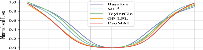
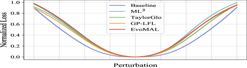
Figure 7: The average 1D loss landscapes generated on the CIFAR-10 dataset, the top figure shows the loss landscapes generated on AllCNN-C, and the bottom figure shows the loss landscapes generated on AlexNet. The landscapes show the average (mean) loss taken across the 5 independent executions of each algorithm on each task+model pair. Best viewed in color.

5.5 Implicit Learning Rate Tuning

Another explanation for why meta-learned loss functions improve performance over handcrafted loss functions is that they can implicitly tune the (base) learning rate since for some suitably expressive representation of $\mathcal{M}$, since

$$\exists\alpha\exists\phi:\theta-\alpha\nabla_{\theta}\mathcal{L}_{\mathcal{T}}\approx\theta-\nabla_{\theta}\mathcal{M}_{\phi}^{\mathsf{T}}.$$ (13)

Thus, performance improvement when using meta-learned loss functions may be the indirect result of a change in the learning rate, scaling the resulting gradient of the loss function. To validate the implicit learning rate hypothesis, a grid search is performed over the base-learning rate using the cross-entropy loss and EvoMAL on CIFAR-10 AllCNN-C. The results are shown in Fig. 8.

The results show that the base learning rate $\alpha$ is a crucial hyper-parameter that influences the performance of both the baseline and EvoMAL. However, in the case of EvoMAL, it is found that when using a relatively small $\alpha$ value, the base learning rate is implicitly tuned, and the loss function learning algorithm achieves an artificially large performance margin compared to the baseline. Implicit learning rate tuning of a similar magnitude is also observed when using relatively large $\alpha$ values; however, the algorithm’s stability is inconsistent, with some runs failing to converge. Finally, when a near-optimal $\alpha$ value is used, performance improvement is consistently better than the baseline. These results indicate two key findings: (1) meta-learned loss functions improve upon handcrafted loss functions and that the performance improvement when using meta-learned loss functions is not primarily a result of implicit learning rate tuning when $\alpha$ is tuned. (2) The base learning rate $\alpha$ can be considered as part of the initialization of the meta-learned loss function, as it determines the initial scale of the loss function.

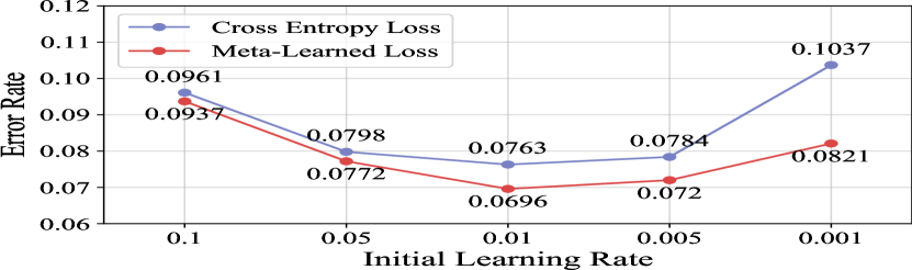
Figure 8: Grid search comparing the average error rate of the baseline cross-entropy loss and EvoMAL on CIFAR-10 AllCNN-C across a set of base learning rate values, where 5 executions of each algorithm are performed on each learning rate value.

6 Conclusions and Future Work

This work presents a new framework for meta-learning symbolic loss function via a hybrid neuro-symbolic search approach called Evolved Model-Agnostic Loss (EvoMAL). The proposed technique uses genetic programming to learn a set of expression tree-based loss functions, which are subsequently transformed into a new network-style representation using a newly proposed transitional procedure. This new representation enables the integration of a computationally tractable gradient-based local-search approach to enhance the search capabilities significantly. Unlike previous approaches, which stack evolution-based techniques, EvoMAL’s efficient local-search enables loss function learning on commodity hardware.

The experimental results confirm that EvoMAL consistently meta-learns loss functions which can produce more performant models compared to those trained with conventional handcrafted loss functions, as well as other state-of-the-art loss function learning techniques. Furthermore, analysis of some of the meta-learned loss functions reveals several key findings regarding common loss function structures and how they interact with the models trained by them. Finally, automating the task of loss function selection has shown to enable a diverse and creative set of loss functions to be generated, which would not be replicable through a simple grid search over handcrafted loss functions.

There are many promising future research directions as a consequence of this work. Regarding algorithmic extensions, the EvoMAL framework is general in its design. It would be interesting to extend it to different meta-learning applications such as gradient-based optimizers or activation functions. In terms of loss function learning, a natural extension of the work would be to meta-learn the loss function and other deep neural network components simultaneously, similar to the methods presented in [92, 93, 17, 94]. For example, the meta-learned loss functions could consider additional arguments such as the timestep or model weights, which would implicitly induce learning rate scheduling or weight regularization, respectively. Another example would be to combine neural architecture search with loss function learning, as the experiments in this work use handcrafted neural network architectures which are biased towards the squared error loss or cross-entropy loss since they were designed to optimize for that specific loss function. Larger performance gains may be achieved using custom neural network architectures explicitly designed for the meta-learned loss functions.

Christian Raymond received a B.Sc. and B.Sc. (Hons) degrees from the School of Engineering and Computer Science, Victoria University of Wellington, New Zealand, in 2020 and 2021 respectively. He is currently pursuing a Ph.D. in Artificial Intelligence with the Evolutionary Computation Research Group (ECRG) at Victoria University of Wellington. His research interests include meta-learning, hyper-parameter optimization, and few-shot learning.

Qi Chen (M’14) received a B.E. degree in Automation from the University of South China, Hunan, China in 2005 and an M.E. degree in Software Engineering from Beijing Institute of Technology, Beijing, China in 2007, and a PhD degree in computer science in 2018 at Victoria University of Wellington, New Zealand. Since 2014, she has joined the Evolutionary Computation Research Group at Victoria University of Wellington (VUW). Currently, she is a Lecturer in the School of Engineering and Computer Science at VUW. Qi’s current research mainly focuses on genetic programming for symbolic regression. Her research interests include machine learning, evolutionary computation, feature selection, feature construction, transfer learning, domain adaptation, and statistical learning theory. She serves as a reviewer of international conferences, including IEEE Congress on Evolutionary Computation, and international journals, including IEEE Transactions on Cybernetics and IEEE Transactions on Evolutionary Computation.

Bing Xue (M’10-SM’21) received the B.Sc. degree from the Henan University of Economics and Law, Zhengzhou, China, in 2007, the M.Sc. degree in management from Shenzhen University, Shenzhen, China, in 2010, and the Ph.D. degree in computer science in 2014 at Victoria University of Wellington (VUW), New Zealand. She is currently a Professor in Computer Science, and Program Director of Science in the School of Engineering and Computer Science at VUW. She has over 300 papers published in fully refereed international journals and conferences and her research focuses mainly on evolutionary computation, machine learning, classification, symbolic regression, feature selection, evolving deep neural networks, image analysis, transfer learning, and multi-objective machine learning. Dr. Xue is currently the Chair of IEEE Computational Intelligence Society (CIS) Task Force on Transfer Learning and Transfer Optimization, Vice-Chair of IEEE CIS Evolutionary Computation Technical Committee, Editor of IEEE CIS Newsletter, Vice-Chair of IEEE Task Force on Evolutionary Feature Selection and Construction, and Vice-Chair IEEE CIS Task Force on Evolutionary Deep Learning and Applications. She has also served asassociate editor of several international journals, such as IEEE Computational Intelligence Magazine and IEEE Transactions on Evolutionary Computation.

Mengjie Zhang (M’04-SM’10-F’19) received the B.E. and M.E. degrees from the Artificial Intelligence Research Center, Agricultural University of Hebei, Hebei, China, and the Ph.D. degree in computer science from RMIT University, Melbourne, VIC, Australia, in 1989, 1992, and 2000, respectively. He is currently a Professor of Computer Science, Head of the Evolutionary Computation Research Group, and the Associate Dean (Research and Innovation) in the Faculty of Engineering. His current research interests include evolutionary computation, particularly genetic programming, particle swarm optimization, and learning classifier systems with application areas of image analysis, multiobjective optimization, feature selection and reduction, job shop scheduling, and transfer learning. He has published over 600 research papers in refereed international journals and conferences. Prof. Zhang is a Fellow of the Royal Society of New Zealand and has been a Panel Member of the Marsden Fund (New Zealand Government Funding), a Fellow of IEEE, and a member of ACM. He was the chair of the IEEE CIS Intelligent Systems and Applications Technical Committee, and chair for the IEEE CIS Emergent Technologies Technical Committee, the Evolutionary Computation Technical Committee, and a member of the IEEE CIS Award Committee. He is a vice-chair of the IEEE CIS Task Force on Evolutionary Feature Selection and Construction, a vice-chair of the Task Force on Evolutionary Computer Vision and Image Processing, and the founding chair of the IEEE Computational Intelligence Chapter in New Zealand. He is also a committee member of the IEEE NZ Central Section.

Appendix A Theoretical Analysis

Inspired by the seminal analysis performed in [95], we analyze the learned loss function from two different perspectives: (1) initial learning behaviors at the null epoch when learning begins under a random initialization, and (2) in the zero training error regime where a loss functions regularization behaviors can be observed when there is nothing new to learn from the training data. The analysis reveals important connections to the cross-entropy loss and label smoothing.

A.1 Learning Rule Decomposition

To begin, we first decompose our learning rule to isolate the contribution of the loss function. For simplicity, we will consider the simple case of using vanilla stochastic gradient descent (SGD). Repeating the update rule shown in Equation (1) of the main manuscript:

$$\theta\leftarrow\theta-\alpha\nabla_{\theta}\Big{[}\mathcal{L}(y,f_{\theta}(x))\Big{]}$$ (14)

where $\alpha$ is the (base) learning rate and $\mathcal{L}$ is the loss function, which takes as arguments the true label $y$ and the base model predictions $f_{\theta}(x)$. Consequently, the update rule for a singular weight $\theta_{j}$ based on the $k^{th}$ model output $f_{\theta}(x)_{k}$ and target $y_{k}$ can be described as follows:

$$\begin{split}\theta_{j}&\leftarrow\theta_{j}-\alpha\frac{\partial}{\partial\theta_{j}}\Big{[}\mathcal{L}(y_{k},f_{\theta}(x)_{k})\Big{]}\\ &=\theta_{j}-\alpha\bigg{[}\frac{\partial}{\partial f}\mathcal{L}(y_{k},f_{\theta}(x)_{k})\cdot\frac{\partial}{\partial\theta_{j}}f_{\theta}(x)_{k}\bigg{]}\\ &=\theta_{j}+\alpha\bigg{[}\underbrace{-\bigg{(}\frac{\partial}{\partial f}\mathcal{L}(y_{k},f_{\theta}(x)_{k})\bigg{)}}_{\gamma}\cdot\frac{\partial}{\partial\theta_{j}}f_{\theta}(x)_{k}\bigg{]}\end{split}$$ (15)

Given this general form, we can now substitute any loss function into Equation (15) to give a unique expression $\gamma$ which describes the behavior of the loss function.

A.2 Learned Loss Functions

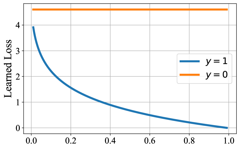
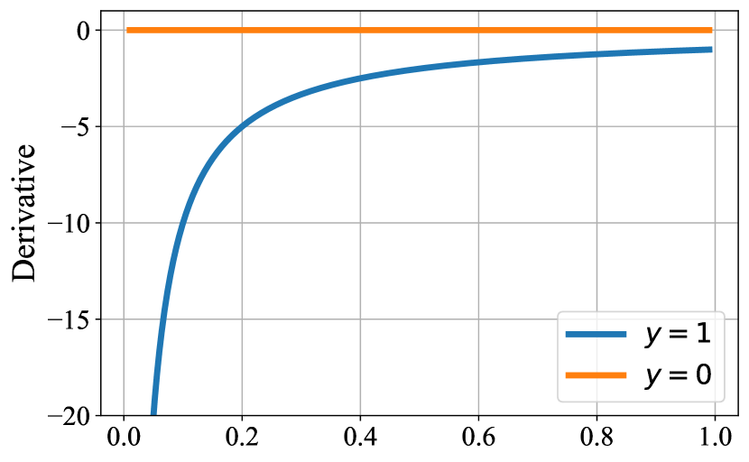
Figure 9: Visualizing the learned loss function $\mathcal{M}_{\phi}$ (left) and its corresponding derivative (right).
The x-axis represents the model’s predictions $f_{\theta}(x)$.

In this section, we analyze the behavior of the handcrafted cross-entropy loss $\mathcal{L}_{CE}=y\cdot\log(f_{\theta}(x))$ and contrast it to a loss function meta-learned by EvoMAL. In particular, we analyze the general form of loss functions a) and e) from Table 6 of the main manuscript (where $\epsilon=1e-7$ is a small constant):

$$\mathcal{M}_{a}=|\log(\sqrt{y\cdot f_{\theta}(x)+\epsilon})|$$ (16)

$$\mathcal{M}_{e}=|\log((y\cdot f_{\theta}(x)+\epsilon)^{2})|$$ (17)

Where $\mathcal{M}_{a}$ and $\mathcal{M}_{e}$ are equivalent upto a scaling factor $\phi_{0}$, since

$$|\log((y\cdot f_{\theta}(x)+\epsilon)^{\phi_{0}})|=\phi_{0}\cdot|\log(y\cdot f_{\theta}(x)+\epsilon)|.$$ (18)

Therefore, the general form of the loss function shown in Fig. 9 can be given as follows where the meta parameters $\phi_{0}$ and $\phi_{1}$ have been made explicit as they are crucial to understanding the behavior of the loss function.

$$\mathcal{M}_{\phi}=\phi_{0}|\log(\phi_{1}(y\cdot f_{\theta}(x)+\epsilon))|$$ (19)

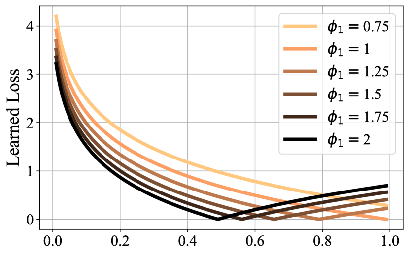
Figure 10: Visualizing the learned loss function $\mathcal{M}_{\phi}$, where the effect of varying $\phi_{0}$ (left) and $\phi_{1}$ (right) are shown.
The x-axis represents the model’s predictions $f_{\theta}(x)$.

A.2.1 Rule Decomposition’s

Substituting the Cross-Entropy ($\mathcal{L}_{CE}$) loss into Equation 2:

$$\theta_{j}\leftarrow\theta_{j}+\alpha\bigg{[}\underbrace{\bigg{(}\frac{\partial}{\partial f}(y_{k}\cdot\log(f_{\theta}(x)_{k})\bigg{)}}_{\gamma_{\mathcal{L}_{CE}}}\frac{\partial}{\partial\theta_{j}}f_{\theta}(x)_{k}\bigg{]}$$ (20)

where the behavior is defined as follows:

$$\gamma_{\mathcal{L}_{CE}}=\frac{y_{k}}{f_{\theta}(x)_{k}}$$ (21)

Substituting the the learned loss function $\mathcal{M}_{\phi}$ into Equation 2:

where the behavior is defined as follows:

A.3 Behavior at the Null Epoch

First, consider the case where the base model weights $\theta$ are randomly initialized (i.e. the null epoch before any training has happened) such that the expected value of the $k^{th}$ output of the model (post softmax/sigmoid) is

$$\forall k\in[1,\mathcal{C}],\text{where }\mathcal{C}\geq 2:\mathbb{E}[f_{\theta}(x)_{k}]=\mathcal{C}^{-1}$$ (24)

where $\mathcal{C}$ is the number of classes/output nodes. Behavior at the null epoch can then be defined piecewise for target vs non-target outputs for each loss function.

In the case of the Cross-Entropy Loss ($\mathcal{L}_{CE}$),

$$\gamma_{\mathcal{L}_{CE}}=\begin{cases}0,&y_{k}=0\\ \mathcal{C},&y_{k}=1\end{cases}$$ (25)

When $y_{k}=1$ the target output value is maximized, while the non-target output values remain the same; however, due to the base model’s softmax output activation function, the target output value being maximized will in turn minimize the non-target outputs.

In the case of the Learned Loss ($\mathcal{M}_{\phi}$),

$$\gamma_{\mathcal{M}_{\phi}}=\begin{cases}-\phi_{0}\frac{0}{\epsilon\cdot\log(\phi_{1}\cdot\epsilon)},&y_{k}=0\\ -\phi_{0}\frac{\log(\phi_{1}(\mathcal{C}^{-1}+\epsilon))}{(\mathcal{C}^{-1}+\epsilon)\cdot|\log(\phi_{1}(\mathcal{C}^{-1}+\epsilon))|},&y_{k}=1\end{cases}$$ (26)

For simplicity, consider the case where the meta-parameters $\phi$ are not optimized and instead left as their default values (i.e. $\phi_{0},\phi_{1}=1$) and let $\epsilon\rightarrow 0$, then for $\mathcal{C}\geq 2$ we get the following expression:

$$\begin{split}\gamma_{\mathcal{M}_{\phi}}&=\begin{cases}-\frac{0}{\epsilon\cdot\log(\epsilon)},&y_{k}=0\\ -\frac{\log(\mathcal{C}^{-1}+\epsilon)}{(\mathcal{C}^{-1}+\epsilon)\cdot|\log(\mathcal{C}^{-1}+\epsilon)|},&y_{k}=1\end{cases}\\ &\xrightarrow[\epsilon\rightarrow 0]{}\begin{cases}0,&y_{k}=0\\ \mathcal{C},&y_{k}=1\end{cases}\end{split}$$ (27)

As shown the learned loss function with a default parameterization is approximately equivalent in learning behavior to that of the cross-entropy loss shown in Equation 25. When $y_{k}=1$ the target output value is maximized, see Fig. 11, while the non-target value is minimized due to the base models softmax. This result shows that at the null epoch, the learned loss function performs approximately equivalently to the cross-entropy loss.

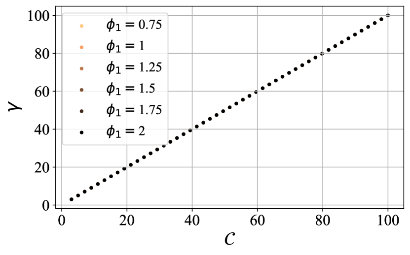
(a) Behavior at the null epoch.

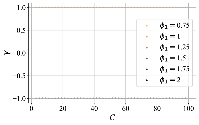
(b) Behavior at zero training error.

Figure 11: Visualizing the behavior $\gamma_{\mathcal{M}_{\phi}}$ of the learned loss function $\mathcal{M}_{\phi}$ where $y_{k}=1$. Plot (a) shows behavior at
the null epoch and (b) shows the behavior when approaching zero training error.

A.4 Behavior at Zero Training Error

Next, the zero training error regime is considered, which explores what happens when there is nothing left to learn from the training data. This regime is of interest as the regularization behavior (or lack thereof) can be observed and contrasted. To analyze the zero training error case $f_{\theta}(x)_{k}$ can be substituted $y_{k}$. However, this results in an indeterminate form (i.e. $0/0$) for the cross-entropy loss when $f_{\theta}(x)=0$ for the non-target output. Therefore, we instead consider the case where $f_{\theta}(x)=\epsilon$ where $\epsilon\rightarrow 0$. Since all the outputs sum to $1$, $f_{\theta}(x)=1-\epsilon(\mathcal{C}-1)$ for the target output and $f_{\theta}(x)=\epsilon$ for the non-target output.

In the case of the Cross Entropy Loss ($\mathcal{L}_{CE}$):

$$\begin{split}\gamma_{\mathcal{L}_{CE}}&=\begin{cases}y_{k}/\epsilon,&y_{k}=0\\ y_{k}/(1-\epsilon(\mathcal{C}-1)),&y_{k}=1\end{cases}\\ &\xrightarrow[\epsilon\rightarrow 0]{}\begin{cases}0,&y_{k}=0\\ 1,&y_{k}=1\end{cases}\end{split}$$ (28)

The target output value is again maximized, while the non-target output values are minimized due to the softmax.

In the case of the Learned Loss ($\mathcal{M}_{\phi}$):

For simplicity, again setting the meta-parameters $\phi_{0},\phi_{1}=1$, and $\epsilon\rightarrow 0$, then for $\mathcal{C}\geq 2$ we get the following expression:

$$\begin{split}\gamma_{\mathcal{M}_{\phi}}&=\begin{cases}-\frac{0}{\epsilon|\log(\epsilon)|},&y_{k}=0\\ -\frac{\log(1-\epsilon(\mathcal{C}-1)+\epsilon)}{(1-\epsilon(\mathcal{C}-1)+\epsilon)|\log(1-\epsilon(\mathcal{C}-1)+\epsilon)|},&y_{k}=1\end{cases}\\ &\xrightarrow[\epsilon\rightarrow 0]{}\begin{cases}0,&y_{k}=0\\ 1,&y_{k}=1\end{cases}\end{split}$$ (30)

When the default parameters (i.e., $\phi_{0},\phi_{1}=1$) are used in the learned loss function, the target output value will be maximized, and the non-target outputs will be minimized similar to the cross-entropy loss, due to the softmax. This indicates that the learned loss function has nearly identical training behavior to the handcrafted cross-entropy loss when using the default parameterization. However, in the following section, we examine the case where the default parameterization is not employed.

A.5 Implicit Label Smoothing

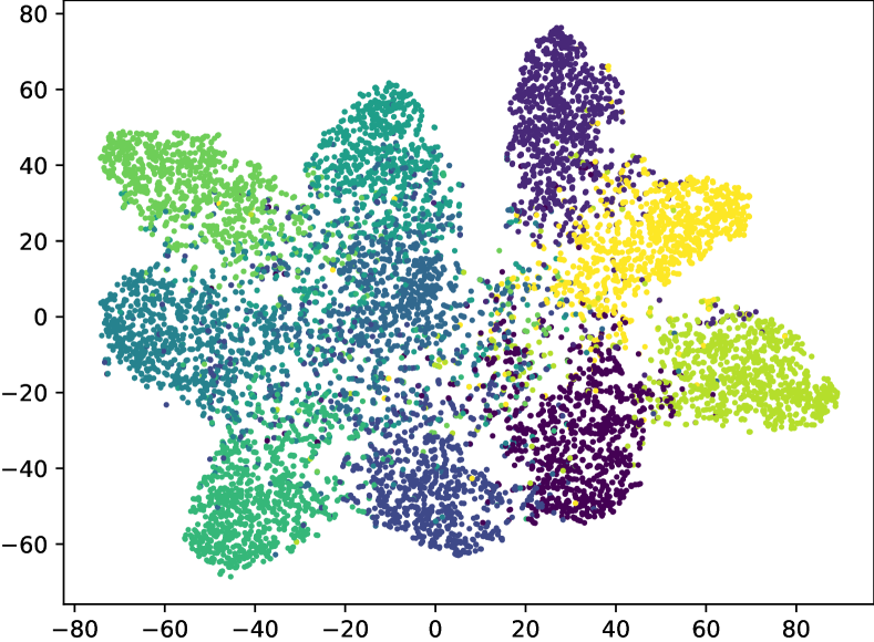
(a) Cross-Entropy (CE) Loss – 15.66%.

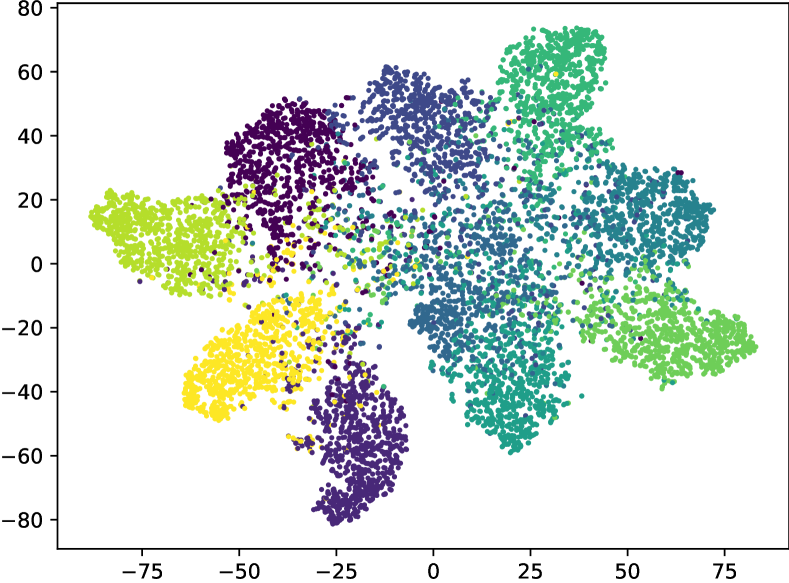
(b) Learned Loss ($\phi_{1}=1$) – 15.43%.

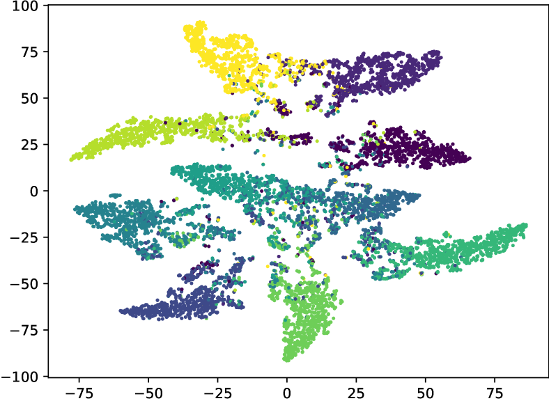
(c) CE + Label Smoothing – 14.99%

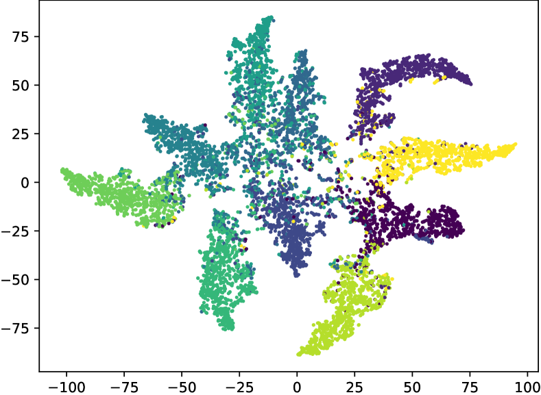
(d) Learned Loss ($\phi_{1}=1.1$) – 14.92%

Figure 12: Visualization of the penultimate layer’s representation on AlexNet CIFAR-10 (testing set), using t-SNE for dimensionality reduction. Color represents the class of an instance.

As shown in Fig. 10, when $\phi_{1}>0$ the behavior of the loss function as the zero training error case is approached changes significantly. Specifically, when $\phi_{1}>0$ the behavior $\gamma_{\mathcal{M}_{\phi}}$ can be characterized as follows:

This shows that when $\phi_{1}>0$ the learned loss function switches from maximizing the target output value to instead minimizing it. Consequently, due to the softmax, this results in the non-target outputs being maximized. This unintuitive learned behavior has appeared previously in other loss functions meta-learned by GLO [28] and TaylorGLO [25] and is a type of regularization strategy. In particular, it has similar behavior to the cross-entropy loss with label smoothing ($\mathcal{L}_{LS}$) [84, 85], which is a method for converting hard targets into soft targets, i.e., $y_{k}\leftarrow y_{k}(1-\psi)+\psi/\mathcal{C}$, where $1\geq\psi>0$ and $\mathcal{C}\geq 2$, preventing the network from becoming over-confident. To demonstrate this parity in behavior the learning rule for the cross-entropy loss with label smoothing is decomposed by substitution into Equation (15):

where the behavior is defined as follows:

$$\gamma_{\mathcal{L}_{LS}}=\frac{y_{k}(1-\psi)+\psi/\mathcal{C}}{f_{\theta}(x)_{k}}$$ (33)

Consequently, we can then analyze the regularization behavior $\gamma_{LS}$ as the zero training error case is approached, where $f_{\theta}(x)=1-\epsilon(\mathcal{C}-1)$ for the target output and $f_{\theta}(x)=\epsilon$ for the non-target output:

Where the $y_{k}=0$ case is shown to dominate $y_{k}=1$ since

$$\frac{\psi}{\epsilon\cdot\mathcal{C}}>(1-\psi)+\frac{\psi}{\mathcal{C}}.$$ (35)

Hence the non-target output is maximized, while the target output is minimized which is identical behavior to $\gamma_{\mathcal{M}_{\phi}}$ when the zero training error case is approached. This key finding suggests that the learned loss function $\mathcal{M}_{\phi}$ where $\phi_{1}>1$ has similar regularization behavior to the cross entropy loss with label smoothing.

Although similar in behavior, it is interesting to note that the learned loss function only needs to be computed on the target output (i.e. 1 loss evaluation per instance), as it is 0 for all non-target outputs, as shown in Equations (27) and (30). In contrast, the cross-entropy loss with label smoothing must be applied to both the target output and all non-target outputs (i.e. $\mathcal{C}$ loss evaluation per instance) as shown in Equation (34). Hence, the learned loss function can be computed significantly faster than the cross-entropy with label smoothing.

A.6 Further Analysis

To further validate these theoretical findings, we analyze the penultimate layer representation of AlexNet on CIFAR-10 when trained with the cross entropy loss with and without label smoothing, and the learned loss function with $\phi_{1}$ set to $1$ and $1.1$. The results are shown in Fig. 12.

Analyzing the results it is shown that the representations learned by (a) the cross-entropy loss and (b) the learned loss function when $\phi=1$ are visually very similar, supporting the findings in Sections A.3 and A.4. Furthermore, analyzing the learned representations by (c) the cross-entropy loss with label smoothing and (d) the learned loss function when $\phi_{1}=1.1$ it can be observed that both the learned representations have better discriminative inter-class representations and tighter intra-class representations. These findings support the finding in the prior section which show similar regularization behavior between the cross-entropy loss with label smoothing and the learned loss function when $\phi_{1}>1$.

A.7 Summary of Findings

Summarizing the findings of this analysis we can conclude:

• With a default parameterization $\phi_{0},\phi_{1}=1$ the behavior of the learned loss function $\gamma_{\mathcal{M}_{\phi}}$ at the null epoch and as the zero error case is approached is identical to the behavior of the cross entropy loss $\gamma_{CE}$.

• When $\phi_{1}>1$ the learned loss function behavior $\gamma_{\mathcal{M}_{\phi}}$ when approaching the zero training error case is identical to the cross-entropy loss with label smoothing $\gamma_{LS}$.

• Further analysis is performed by visualizing the learned representations on AlexNet CIFAR-10, which shows that the theoretical findings are consistent with the empirical findings, as similar behavior is observed in the learned representations.

Appendix B Hyperparameter Sensitivity Analysis

B.1 Meta-Gradient Steps

The number of meta-gradient steps $\mathcal{S}_{meta}$ in EvoMAL was determined via a grid search early into the development. We have found that EvoMAL is not particularly sensitive to the choice of $\mathcal{S}_{meta}$, as shown by the results in Fig. 13, which contrasts the error rate when increasing and decreasing the number of meta-gradient steps on MNIST+LeNet-5. The results show that there are many feasible values of $\mathcal{S}_{meta}$ and values greater than $\mathcal{S}_{meta}\geq 250$ produce strong performance compared to the benchmark methods.

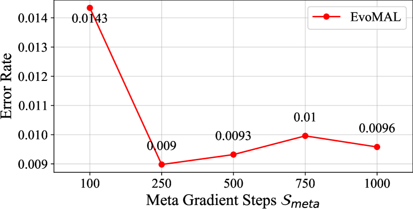
Figure 13: Grid search comparing the average error rate of EvoMAL on MNIST LeNet-5 across a set of meta-gradient step values $\mathcal{S}_{meta}=\{100,250,500,750,1000\}$, where 5 executions are performed on each meta-gradient step value.

B.2 Short-Horizon Bias and Partial Training Sessions

TABLE VII: Results reporting the mean $\pm$ standard deviation final inference testing error rate across 5 independent executions of EvoMAL on each of the testing-gradient step values.

Task and Model	EvoMAL
MNIST
LeNet-5 ($\mathcal{S}_{testing}=500$)	0.0090 $\pm$ 0.0003
LeNet-5 ($\mathcal{S}_{testing}=10,000$)	0.0098 $\pm$ 0.0010

In EvoMAL the learned loss functions fitnesses are evaluated using a partial training session (i.e. using a truncated number of gradient steps $\mathcal{S}_{testing}$). Partial training sessions can be used in this context as performance at the beginning of training is highly correlated with the performance at the end of training, as noted in the ICLR2021 OpenReview version of [25], in Appendix D entitled ”MNIST Evaluation Length Sensitivity”, which showed empirically that in the context of loss function learning you could reduce the evaluation length (i.e. $\mathcal{S}_{testing}$) to 1% of the full training session and the final results would be near identical (99.46% vs 99.45% accuracy using their custom CNN architecture).

We independently reproduce these results on MNIST + LeNet-5 using EvoMAL with $\mathcal{S}_{testing}=10,000$, extending the loss function fitness evaluation to the full duration of the training session taken at meta-testing time. The results reported in Table VII show no significant degradation in performance when reducing the evaluation length in EvoMAL to a partial training session of $\mathcal{S}_{testing}=500$.

Evaluating the fitness $\mathcal{F}$ after a partial training session will always result in some short-horizon bias [66]; however, it should be noted that evolution-based loss function learning methods such as EvoMAL do not suffer nearly as much short-horizon bias as methods that exclusively rely on unrolled differentiation for optimization (e.g., ML³) [24]. In unrolled differentiation, the intermediate iterates (i.e., optimization path) need to be stored in memory; thus, the number of base gradient steps is limited to very few, typically in the low double digits [13]. In contrast, evolution-based methods do not need to store the intermediate iterates, thus, can take many more steps, typically in the hundreds or low thousands, which is an order-of-magnitude longer horizon.

Appendix C Supplementary Content and Analysis

C.1 Constraint Enforcement

For clarity, both the required arguments constraint and non-negative output constraint enforcement procedures presented in Section 3.2.3 are summarized in Fig. 14.

C.2 Analysis of Search Space Design

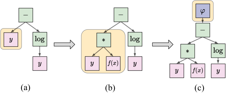
Figure 14: Overview of the constraint enforcement procedure, where (a) is a constraint violating expression, (b) demonstrates enforcing the required arguments constraint, and (c) shows enforcing the non-negative output constraint.

To better understand the effects of the search space design on the learned loss functions developed by EvoMAL, we analyze the best-performing loss functions developed by EvoMAL. In particular, the frequencies of occurrence of the function nodes of the best-performing loss functions from all EvoMAL experiments are presented in Fig. 15. Analyzing the results it is observed that the most frequently recurring loss function sub-structure is the use of the subtraction or multiplication operator, with arguments $y$ and $f_{\theta}(x)$. This result is expected as these are commonly used building blocks in loss functions for computing the error in regression and classification, respectively. There is also high usage of the square root and square operators, which are commonly used for scaling the effects of large and small errors to either penalize or discount different groups of predictions (i.e. inliers and outliers). Finally, there is minimal usage of the $sign$, $min$, and $tanh$ operators, which empirically suggests that these function nodes are seldom important to the design of learned loss functions, and that future studies may wish to consider removing them from the function set to increase the search efficiency.

Figure 15: Frequencies of the primitive mathematical operations in the symbolic loss functions discovered by EvoMAL across all datasets and random seeds.

References

- [1] J. Vanschoren, “Meta-learning: A survey,” arXiv preprint arXiv:1810.03548, 2018.
- [2] H. Peng, “A comprehensive overview and survey of recent advances in meta-learning,” arXiv preprint arXiv:2004.11149, 2020.
- [3] T. Hospedales, A. Antoniou, P. Micaelli, and A. Storkey, “Meta-learning in neural networks: A survey,” IEEE Transactions on Pattern Analysis and Machine Intelligence, vol. 44, no. 9, pp. 5149–5169, 2022.
- [4] H. Altae-Tran, B. Ramsundar, A. S. Pappu, and V. Pande, “Low data drug discovery with one-shot learning,” ACS central science, vol. 3, no. 4, pp. 283–293, 2017.
- [5] A. Ignatov, R. Timofte, A. Kulik, S. Yang, K. Wang, F. Baum, M. Wu, L. Xu, and L. Van Gool, “Ai benchmark: All about deep learning on smartphones in 2019,” in 2019 IEEE/CVF International Conference on Computer Vision Workshop (ICCVW). IEEE, 2019, pp. 3617–3635.
- [6] J. Schmidhuber, “Evolutionary principles in self-referential learning,” Ph.D. dissertation, Technische Universität München, 1987.
- [7] ——, “Learning to control fast-weight memories: An alternative to dynamic recurrent networks,” Neural Computation, vol. 4, no. 1, pp. 131–139, 1992.
- [8] S. Bengio, Y. Bengio, and J. Cloutier, “Use of genetic programming for the search of a new learning rule for neural networks,” in Proceedings of the First IEEE Conference on Evolutionary Computation. IEEE World Congress on Computational Intelligence. IEEE, 1994, pp. 324–327.
- [9] M. Andrychowicz, M. Denil, S. Gomez, M. W. Hoffman, D. Pfau, T. Schaul, B. Shillingford, and N. De Freitas, “Learning to learn by gradient descent by gradient descent,” in Advances in neural information processing systems, 2016, pp. 3981–3989.
- [10] P. Ramachandran, B. Zoph, and Q. V. Le, “Searching for activation functions,” arXiv preprint arXiv:1710.05941, 2017.
- [11] C. Finn, P. Abbeel, and S. Levine, “Model-agnostic meta-learning for fast adaptation of deep networks,” in International Conference on Machine Learning. PMLR, 2017, pp. 1126–1135.
- [12] A. Nichol, J. Achiam, and J. Schulman, “On first-order meta-learning algorithms,” arXiv preprint arXiv:1803.02999, 2018.
- [13] A. Rajeswaran, C. Finn, S. M. Kakade, and S. Levine, “Meta-learning with implicit gradients,” Advances in neural information processing systems, vol. 32, 2019.
- [14] X. Song, W. Gao, Y. Yang, K. Choromanski, A. Pacchiano, and Y. Tang, “Es-maml: Simple hessian-free meta learning,” arXiv preprint arXiv:1910.01215, 2019.
- [15] J. Kim, S. Lee, S. Kim, M. Cha, J. K. Lee, Y. Choi, Y. Choi, D.-Y. Cho, and J. Kim, “Auto-meta: Automated gradient based meta learner search,” arXiv preprint arXiv:1806.06927, 2018.
- [16] K. O. Stanley, J. Clune, J. Lehman, and R. Miikkulainen, “Designing neural networks through neuroevolution,” Nature Machine Intelligence, vol. 1, no. 1, pp. 24–35, 2019.
- [17] T. Elsken, B. Staffler, J. H. Metzen, and F. Hutter, “Meta-learning of neural architectures for few-shot learning,” in Proceedings of the IEEE/CVF conference on computer vision and pattern recognition, 2020, pp. 12 365–12 375.
- [18] Y. Ding, Y. Wu, C. Huang, S. Tang, Y. Yang, L. Wei, Y. Zhuang, and Q. Tian, “Learning to learn by jointly optimizing neural architecture and weights,” in Proceedings of the IEEE/CVF Conference on Computer Vision and Pattern Recognition, 2022, pp. 129–138.
- [19] E. Real, C. Liang, D. So, and Q. Le, “Automl-zero: Evolving machine learning algorithms from scratch,” in International Conference on Machine Learning. PMLR, 2020, pp. 8007–8019.
- [20] J. D. Co-Reyes, Y. Miao, D. Peng, E. Real, S. Levine, Q. V. Le, H. Lee, and A. Faust, “Evolving reinforcement learning algorithms,” arXiv preprint arXiv:2101.03958, 2021.
- [21] Q. Wang, Y. Ma, K. Zhao, and Y. Tian, “A comprehensive survey of loss functions in machine learning,” Annals of Data Science, vol. 9, no. 2, pp. 187–212, 2022.
- [22] D. E. Rumelhart, G. E. Hinton, and R. J. Williams, “Learning representations by back-propagating errors,” nature, vol. 323, no. 6088, pp. 533–536, 1986.
- [23] D. H. Wolpert and W. G. Macready, “No free lunch theorems for optimization,” IEEE transactions on evolutionary computation, vol. 1, no. 1, pp. 67–82, 1997.
- [24] S. Bechtle, A. Molchanov, Y. Chebotar, E. Grefenstette, L. Righetti, G. Sukhatme, and F. Meier, “Meta-learning via learned loss,” in 2020 25th International Conference on Pattern Recognition (ICPR). IEEE, 2021, pp. 4161–4168.
- [25] S. Gonzalez and R. Miikkulainen, “Optimizing loss functions through multi-variate taylor polynomial parameterization,” in Proceedings of the Genetic and Evolutionary Computation Conference, 2021, pp. 305–313.
- [26] B. Gao, H. Gouk, and T. M. Hospedales, “Searching for robustness: Loss learning for noisy classification tasks,” in Proceedings of the IEEE/CVF International Conference on Computer Vision, 2021, pp. 6670–6679.
- [27] B. Gao, H. Gouk, Y. Yang, and T. Hospedales, “Loss function learning for domain generalization by implicit gradient,” in International Conference on Machine Learning. PMLR, 2022, pp. 7002–7016.
- [28] S. Gonzalez and R. Miikkulainen, “Improved training speed, accuracy, and data utilization through loss function optimization,” in 2020 IEEE Congress on Evolutionary Computation (CEC). IEEE, 2020, pp. 1–8.
- [29] P. Liu, G. Zhang, B. Wang, H. Xu, X. Liang, Y. Jiang, and Z. Li, “Loss function discovery for object detection via convergence-simulation driven search,” in ICLR, 2020.
- [30] H. Li, T. Fu, J. Dai, H. Li, G. Huang, and X. Zhu, “Autoloss-zero: Searching loss functions from scratch for generic tasks,” in Proceedings of the IEEE/CVF Conference on Computer Vision and Pattern Recognition, 2022, pp. 1009–1018.
- [31] J. R. Koza, Genetic programming: on the programming of computers by means of natural selection. MIT press, 1992, vol. 1.
- [32] D. Maclaurin, D. Duvenaud, and R. Adams, “Gradient-based hyperparameter optimization through reversible learning,” in International conference on machine learning. PMLR, 2015, pp. 2113–2122.
- [33] E. Grefenstette, B. Amos, D. Yarats, P. M. Htut, A. Molchanov, F. Meier, D. Kiela, K. Cho, and S. Chintala, “Generalized inner loop meta-learning,” arXiv preprint arXiv:1910.01727, 2019.
- [34] J. Grabocka, R. Scholz, and L. Schmidt-Thieme, “Learning surrogate losses,” arXiv preprint arXiv:1905.10108, 2019.
- [35] C. Huang, S. Zhai, W. Talbott, M. B. Martin, S.-Y. Sun, C. Guestrin, and J. Susskind, “Addressing the loss-metric mismatch with adaptive loss alignment,” in International Conference on Machine Learning. PMLR, 2019, pp. 2891–2900.
- [36] R. Houthooft, Y. Chen, P. Isola, B. Stadie, F. Wolski, O. Jonathan Ho, and P. Abbeel, “Evolved policy gradients,” in Advances in Neural Information Processing Systems, vol. 31, 2018, pp. 5405–5414.
- [37] L. Wu, F. Tian, Y. Xia, Y. Fan, T. Qin, L. Jian-Huang, and T.-Y. Liu, “Learning to teach with dynamic loss functions,” Advances in Neural Information Processing Systems, vol. 31, 2018.
- [38] A. Antoniou and A. J. Storkey, “Learning to learn by self-critique,” Advances in Neural Information Processing Systems, vol. 32, 2019.
- [39] L. Kirsch, S. van Steenkiste, and J. Schmidhuber, “Improving generalization in meta reinforcement learning using learned objectives,” arXiv preprint arXiv:1910.04098, 2019.
- [40] A. Collet, A. Bazco-Nogueras, A. Banchs, and M. Fiore, “Loss meta-learning for forecasting,” 2022. [Online]. Available: https://openreview.net/forum?id=rczz7TUKIIB
- [41] Z. Leng, M. Tan, C. Liu, E. D. Cubuk, X. Shi, S. Cheng, and D. Anguelov, “Polyloss: A polynomial expansion perspective of classification loss functions,” Tenth International Conference on Learning Representations, 2022.
- [42] C. Raymond, Q. Chen, B. Xue, and M. Zhang, “Online Loss Function Learning,” arXiv e-prints, p. arXiv:2301.13247, Jan. 2023.
- [43] Y. Balaji, S. Sankaranarayanan, and R. Chellappa, “Metareg: Towards domain generalization using meta-regularization,” Advances in Neural Information Processing Systems, vol. 31, pp. 998–1008, 2018.
- [44] J. T. Barron, “A general and adaptive robust loss function,” in Proceedings of the IEEE/CVF Conference on Computer Vision and Pattern Recognition, 2019, pp. 4331–4339.
- [45] Y. Li, Y. Yang, W. Zhou, and T. Hospedales, “Feature-critic networks for heterogeneous domain generalisation,” in International Conference on Machine Learning. PMLR, 2019, pp. 3915–3924.
- [46] A. F. Psaros, K. Kawaguchi, and G. E. Karniadakis, “Meta-learning pinn loss functions,” Journal of Computational Physics, vol. 458, p. 111121, 2022.
- [47] A. Topchy and W. F. Punch, “Faster genetic programming based on local gradient search of numeric leaf values,” in Proceedings of the genetic and evolutionary computation conference (GECCO-2001), vol. 155162. Morgan Kaufmann, 2001.
- [48] W. Smart and M. Zhang, “Applying online gradient descent search to genetic programming for object recognition,” in Proceedings of the second workshop on Australasian information security, Data Mining and Web Intelligence, and Software Internationalisation-Volume 32, 2004, pp. 133–138.
- [49] M. Zhang and W. Smart, “Learning weights in genetic programs using gradient descent for object recognition,” in Workshops on Applications of Evolutionary Computation. Springer, 2005, pp. 417–427.
- [50] R. E. Wengert, “A simple automatic derivative evaluation program,” Communications of the ACM, vol. 7, no. 8, pp. 463–464, 1964.
- [51] J. Domke, “Generic methods for optimization-based modeling,” in Artificial Intelligence and Statistics. PMLR, 2012, pp. 318–326.
- [52] C.-A. Deledalle, S. Vaiter, J. Fadili, and G. Peyré, “Stein unbiased gradient estimator of the risk (sugar) for multiple parameter selection,” SIAM Journal on Imaging Sciences, vol. 7, no. 4, pp. 2448–2487, 2014.
- [53] S. Gonzalez et al., “Improving deep learning through loss-function evolution,” Ph.D. dissertation, 2020.
- [54] B. Gao, “Meta-learning to optimise: loss functions and update rules,” 2023.
- [55] J. Ni, R. H. Drieberg, and P. I. Rockett, “The use of an analytic quotient operator in genetic programming,” IEEE Transactions on Evolutionary Computation, vol. 17, no. 1, pp. 146–152, 2012.
- [56] Q. Chen, B. Xue, and M. Zhang, “Generalisation and domain adaptation in gp with gradient descent for symbolic regression,” in 2015 IEEE congress on evolutionary computation (CEC). IEEE, 2015, pp. 1137–1144.
- [57] L. Franceschi, M. Donini, P. Frasconi, and M. Pontil, “Forward and reverse gradient-based hyperparameter optimization,” in International Conference on Machine Learning. PMLR, 2017, pp. 1165–1173.
- [58] L. Franceschi, P. Frasconi, S. Salzo, R. Grazzi, and M. Pontil, “Bilevel programming for hyperparameter optimization and meta-learning,” in International Conference on Machine Learning. PMLR, 2018, pp. 1568–1577.
- [59] A. Shaban, C.-A. Cheng, N. Hatch, and B. Boots, “Truncated back-propagation for bilevel optimization,” in The 22nd International Conference on Artificial Intelligence and Statistics. PMLR, 2019, pp. 1723–1732.
- [60] D. Scieur, Q. Bertrand, G. Gidel, and F. Pedregosa, “The curse of unrolling: Rate of differentiating through optimization,” arXiv preprint arXiv:2209.13271, 2022.
- [61] P. Wong and M. Zhang, “Algebraic simplification of gp programs during evolution,” in Proceedings of the 8th annual conference on Genetic and evolutionary computation, 2006, pp. 927–934.
- [62] D. Kinzett, M. Johnston, and M. Zhang, “Numerical simplification for bloat control and analysis of building blocks in genetic programming,” Evolutionary Intelligence, vol. 2, pp. 151–168, 2009.
- [63] N. Javed, F. Gobet, and P. Lane, “Simplification of genetic programs: a literature survey,” Data Mining and Knowledge Discovery, vol. 36, no. 4, pp. 1279–1300, 2022.
- [64] J. J. Grefenstette and J. M. Fitzpatrick, “Genetic search with approximate function evaluations,” in Proceedings of an International Conference on Genetic Algorithms and Their Applications, 1985, pp. 112–120.
- [65] Y. Jin, “Surrogate-assisted evolutionary computation: Recent advances and future challenges,” Swarm and Evolutionary Computation, vol. 1, no. 2, pp. 61–70, 2011.
- [66] Y. Wu, M. Ren, R. Liao, and R. Grosse, “Understanding short-horizon bias in stochastic meta-optimization,” arXiv preprint arXiv:1803.02021, 2018.
- [67] F.-A. Fortin, F.-M. De Rainville, M.-A. G. Gardner, M. Parizeau, and C. Gagné, “Deap: Evolutionary algorithms made easy,” The Journal of Machine Learning Research, vol. 13, no. 1, pp. 2171–2175, 2012.
- [68] A. Paszke, S. Gross, F. Massa, A. Lerer, J. Bradbury, G. Chanan, T. Killeen, Z. Lin, N. Gimelshein, L. Antiga et al., “Pytorch: An imperative style, high-performance deep learning library,” Advances in neural information processing systems, vol. 32, pp. 8026–8037, 2019.
- [69] A. Asuncion and D. Newman, “Uci machine learning repository,” 2007.
- [70] Y. LeCun, L. Bottou, Y. Bengio, and P. Haffner, “Gradient-based learning applied to document recognition,” Proceedings of the IEEE, vol. 86, no. 11, pp. 2278–2324, 1998.
- [71] A. Krizhevsky and G. Hinton, “Learning multiple layers of features from tiny images,” 2009.
- [72] Y. Netzer, T. Wang, A. Coates, A. Bissacco, B. Wu, and A. Y. Ng, “Reading digits in natural images with unsupervised feature learning,” NIPS, 2011.
- [73] A. G. Baydin, R. Cornish, D. M. Rubio, M. Schmidt, and F. Wood, “Online learning rate adaptation with hypergradient descent,” in Sixth International Conference on Learning Representations, 2018.
- [74] P. McCullagh, J. A. Nelder et al., Generalized linear models. Routledge, 1989.
- [75] A. Krizhevsky, I. Sutskever, and G. E. Hinton, “Imagenet classification with deep convolutional neural networks,” Advances in neural information processing systems, vol. 25, 2012.
- [76] K. Simonyan and A. Zisserman, “Very deep convolutional networks for large-scale image recognition,” arXiv preprint arXiv:1409.1556, 2014.
- [77] J. T. Springenberg, A. Dosovitskiy, T. Brox, and M. Riedmiller, “Striving for simplicity: The all convolutional net,” arXiv preprint arXiv:1412.6806, 2014.
- [78] K. He, X. Zhang, S. Ren, and J. Sun, “Deep residual learning for image recognition,” in Proceedings of the IEEE conference on computer vision and pattern recognition, 2016, pp. 770–778.
- [79] ——, “Identity mappings in deep residual networks,” in European conference on computer vision. Springer, 2016, pp. 630–645.
- [80] S. Zagoruyko and N. Komodakis, “Wide residual networks,” arXiv preprint arXiv:1605.07146, 2016.
- [81] F. N. Iandola, S. Han, M. W. Moskewicz, K. Ashraf, W. J. Dally, and K. Keutzer, “Squeezenet: Alexnet-level accuracy with 50x fewer parameters and¡ 0.5 mb model size,” arXiv preprint arXiv:1602.07360, 2016.
- [82] D. Han, J. Kim, and J. Kim, “Deep pyramidal residual networks,” in Proceedings of the IEEE conference on computer vision and pattern recognition, 2017, pp. 5927–5935.
- [83] T.-Y. Lin, P. Goyal, R. Girshick, K. He, and P. Dollár, “Focal loss for dense object detection,” in Proceedings of the IEEE international conference on computer vision, 2017, pp. 2980–2988.
- [84] C. Szegedy, V. Vanhoucke, S. Ioffe, J. Shlens, and Z. Wojna, “Rethinking the inception architecture for computer vision,” in Proceedings of the IEEE conference on computer vision and pattern recognition, 2016, pp. 2818–2826.
- [85] R. Müller, S. Kornblith, and G. E. Hinton, “When does label smoothing help?” Advances in neural information processing systems, vol. 32, 2019.
- [86] M. J. Black and A. Rangarajan, “On the unification of line processes, outlier rejection, and robust statistics with applications in early vision,” International journal of computer vision, vol. 19, no. 1, pp. 57–91, 1996.
- [87] S. Hochreiter and J. Schmidhuber, “Flat minima,” Neural computation, vol. 9, no. 1, pp. 1–42, 1997.
- [88] N. S. Keskar, D. Mudigere, J. Nocedal, M. Smelyanskiy, and P. T. P. Tang, “On large-batch training for deep learning: Generalization gap and sharp minima,” arXiv preprint arXiv:1609.04836, 2016.
- [89] H. Li, Z. Xu, G. Taylor, C. Studer, and T. Goldstein, “Visualizing the loss landscape of neural nets,” Advances in neural information processing systems, vol. 31, 2018.
- [90] P. Chaudhari, A. Choromanska, S. Soatto, Y. LeCun, C. Baldassi, C. Borgs, J. Chayes, L. Sagun, and R. Zecchina, “Entropy-sgd: Biasing gradient descent into wide valleys,” Journal of Statistical Mechanics: Theory and Experiment, vol. 2019, no. 12, p. 124018, 2019.
- [91] L. Dinh, R. Pascanu, S. Bengio, and Y. Bengio, “Sharp minima can generalize for deep nets,” in International Conference on Machine Learning. PMLR, 2017, pp. 1019–1028.
- [92] S. Ravi and H. Larochelle, “Optimization as a model for few-shot learning,” in International conference on learning representations, 2017.
- [93] Z. Li, F. Zhou, F. Chen, and H. Li, “Meta-sgd: Learning to learn quickly for few-shot learning,” arXiv preprint arXiv:1707.09835, 2017.
- [94] S. Baik, J. Choi, H. Kim, D. Cho, J. Min, and K. M. Lee, “Meta-learning with task-adaptive loss function for few-shot learning,” in Proceedings of the IEEE/CVF International Conference on Computer Vision, 2021, pp. 9465–9474.
- [95] S. Gonzalez and R. Miikkulainen, “Effective regularization through loss-function metalearning,” arXiv preprint arXiv:2010.00788, 2020.