Gap-ETH-Tight Approximation Schemes for Red-Green-Blue Separation and Bicolored Noncrossing Euclidean Travelling Salesman Tours

In this paper, we study problems of connecting classes of points via noncrossing structures. Given a set of colored terminal points, we want to find a graph for each color that connects all terminals of its color with the restriction that no two graphs cross each other. We consider these problems both on the Euclidean plane and in planar graphs.

On the algorithmic side, we give a Gap-ETH-tight EPTAS for the two-colored traveling salesman problem as well as for the red-blue-green separation problem (in which we want to separate terminals of three colors with two noncrossing polygons of minimum length), both on the Euclidean plane. This improves the work of Arora and Chang (ICALP 2003) who gave a slower PTAS for the simpler red-blue separation problem. For the case of unweighted plane graphs, we also show a PTAS for the two-colored traveling salesman problem. All these results are based on our new patching procedure that might be of independent interest.

On the negative side, we show that the problem of connecting terminal pairs with noncrossing paths is NP-hard on the Euclidean plane, and that the problem of finding two noncrossing spanning trees is NP-hard in plane graphs.

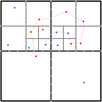
Figure 5: inline]KF: missing reference to this figure?inline]KF: polish the caption. inline]KF: portals of deepest level too small. inline]KF: red tour barely visible. An illustration of the construction of the quadtree for Red-Blue Separation problem. Input points are represented with red/blue circles. The white circles are representation of portals. Note that each boundary boundary of quadtree has exactly the same number of portals. The pink polygon is a portal-respectinginline]KF: we haven’t defined portal-respecting! polygon based on the technique by Arora and Chang [5].

linecolor=blue,backgroundcolor=blue!50,bordercolor=blue,inline](Reviewer’s Comment!)
variables S and R are sometimes slanted and sometimes not linecolor=blue,backgroundcolor=blue!50,bordercolor=blue,inline](Reviewer’s Comment!)
paragraph headings sometimes use title case and sometimes not linecolor=blue,backgroundcolor=blue!50,bordercolor=blue,inline](Reviewer’s Comment!)
X and Y as the axes of the plane are inconsistently capitalized linecolor=blue,backgroundcolor=blue!50,bordercolor=blue,inline](Reviewer’s Comment!)
add figures regarding allowed/disallowed solutions in plane and especially the graph setting. linecolor=blue,backgroundcolor=blue!50,bordercolor=blue,inline](Reviewer’s Comment!)
if quadtree cells can have no points, than update fig 5 accordingly; otherwise make it clear that they always have points. linecolor=blue,backgroundcolor=blue!50,bordercolor=blue,inline](Reviewer’s Comment!)
Make notation consistent! ("That description is hard to verify, due to changing notation.") linecolor=blue,backgroundcolor=blue!50,bordercolor=blue,inline](Reviewer’s Comment!)
define first(!) variables before using them. Bad/good example(?): "if a graph of n vertices has at most two terminals per color, and terminals are adjacent to h faces in total, then the problem can be solved in $2^{O(h^{2})}n\log k$ time. [13]"
309: "context first" is a generalization of “define before using": “For a simple curve $\pi\in\mathbb{R}^{2}$ that contains two points $y$,$z$, we define… (Otherwise the reader thinks of two points, then afterward learns they were supposed to be “on $\pi$”.) linecolor=blue,backgroundcolor=blue!50,bordercolor=blue,inline](Reviewer’s Comment!)
Our "technical tool" really only for 1 of 4 problems needed?? (… keeping the technical description of one tool … that is needed for one of the four problems.) linecolor=blue,backgroundcolor=blue!50,bordercolor=blue,inline](Reviewer’s Comment!)
Using $\mathcal{S}$, $\ell$, and $S$ in close proximity makes this a little hard for your readers as well, by the way.

1 Introduction

linecolor=red,backgroundcolor=red!25,bordercolor=red,inline](Important Todo!)
KF: I would emphasize very much that our results are Gap-ETH-tight! Even in abstract. Imagine that you are given a set of cities on a map belonging to different communities. Your goal is to separate the communities from each other with fences such that each community remains connected. The total length of the fences should be minimized.

linecolor=yellow,backgroundcolor=yellow!8,bordercolor=yellow,inline](Just a note for us)
KF: (For the future) One could study a variant of the problem where we do not want to minimize the fence length but where we want that the areas of the communities have the same size (where e.g. we always have a fixed third cycle that is the convex hull).

Figure 1: Points on the plane are labeled into three groups (red, blue and green) and the task is to find two polygons of total minimum length that separate the three classes. The solution on the left is not feasible because two polygons are crossing. The solution on the right is feasible because polygons are noncrossing and points in different classes are separated.

In this paper, we study the computational complexity of a very general class of problems that can model such and similar questions and we provide efficient algorithms to solve them. Given $n$ colored terminal points (on the Euclidean plane or in a plane graph), the goal is to find a set of pairwise noncrossing geometric graphs of minimum total length that satisfy some requirement for each color. For instance, in the problem mentioned above, we look for noncrossing cycles that separate terminals of different colors.

The study of such noncrossing problems is not only motivated by the fact that these problems are natural generalizations of well-examined fundamental problems (e.g. the spanning tree problem and the traveling salesman problem) that lead to the development of new techniques. Such problems are also motivated by their rich application in different fields, e.g., to VLSI design [37, 38, 24, 14] and set visualization of spatial data [2, 20, 13, 20, 8, 35]. For instance, in a method for visualizing embedded and clustered graphs [13], clusters are visualized by non-overlapping regions that are constructed on top of noncrossing trees connecting the vertices of each cluster. In the following, we introduce the problems and discuss our contribution and related work. At the end, we give an overview of our paper.

Red-Blue-Green Separation

In the Red-Blue-Green Separation problem, we are given a set of $n$ terminal points on the (Euclidean) plane. Each point is assigned to one of three colors (red, blue, or green). The goal is to find two noncrossing Jordan curves that separate terminals of different classes (i.e., every possible path connecting two terminals of different color must cross at least one of the curves) of minimum total length; see Fig. 1 for an illustration.

linecolor=red,backgroundcolor=red!25,bordercolor=red,](Important Todo!)
Add a remark that we look at polygons and not lines

Various forms of this problems have been studied in connection to computer vision and collision avoidance [12, 39, 11, 36], geographic information retrieval [35] or even finding pandemic mitigation strategies [10]. To the best of our knowledge, the problem has been studied only for two colors which is already NP-hard [12]. Mata and Mitchel [27] obtained an $\mathcal{O}(\log n)$-approximation scheme which was subsequently strengthened by an $\mathcal{O}(\log m)$ approximation algorithm by Gudmundsson and Levcopoulos [19] where $m$ is an output-sensitive parameter bounded by $n$. Finally, Arora and Chang [5] proposed an $n(\log n)^{\mathcal{O}(1/\varepsilon)}$-time algorithm that returns a $(1+\varepsilon)$-approximation for any $\varepsilon>0$. The aforementioned approximation schemes crucially rely on patching schemes and other techniques that seem to work only for two colors, where we look only for a single curve. Due to the many new technical challenges arising from the noncrossing constraint, it is not obvious how to generalize these results to more colors, where we want to find pairwise noncrossing curves.

Our contribution is twofold. First, we succeed in generalizing the result of Arora and Chang [5] to three colors by designing, among others, a new patching procedure of independent interest for noncrossing curves. Second, we improve the running time of Arora and Chang [5] tolinecolor=red,backgroundcolor=red!25,bordercolor=red,](Important Todo!)
KF: near-optimal? $2^{\mathcal{O}(1/\varepsilon)}n\,\textup{polylog}(n)$ and thus obtain an EPTAS for three colors.

Theorem 1.1 (Red-Blue-Green Separation).

Euclidean Noncrossing Red-Blue-Green Separation admits a randomized $(1+\varepsilon)$-approximation scheme with $2^{\mathcal{O}(1/\varepsilon)}n\,\textup{polylog}(n)$ running time. linecolor=red,backgroundcolor=red!25,bordercolor=red,inline](Important Todo!)
KF: near-optimal?

We note that our algorithm is near-optimal. Namely, Eades and Rappaport [12] show a reduction of the red-blue separation problem to Euclidean TSP with an arbitrary small gap. This fact combined with a recent lower bound on Euclidean TSP [22] means that an $2^{o(1/\varepsilon)}\mathrm{poly}(n)$-time approximation for Euclidean Noncrossing Red-Blue-Green Separation would contradict Gap-ETH.

Noncrossing Tours

In the Bicolored Noncrossing Traveling Salesman Tours problem, we are given $n$ terminal points on the plane. Each point is colored either red or blue. The task is to find two noncrossing round-trip tours of minimum total length such that all red points are visited by one tour and all blue points are visited by the other one. The problem is a generalization of the classical Euclidean traveling salesman problem [29] and is therefore NP-hard. To the best of our knowledge, this problem has not been considered before in the literature, although it nicely fits into the recent trend of finding noncrossing geometric structures (see, e.g., the works of Polishchuk and Mitchell [32], Bereg et al. [7] and Kostitsyna et al. [23]). By using the same patching procedure as for Theorem 1.1, we obtain an EPTAS for this problem.

Theorem 1.2.

Euclidean Bicolored Noncrossing Traveling Salesman Tours admits a randomized $(1+\varepsilon)$-approximation scheme with $2^{\mathcal{O}(1/\varepsilon)}n\,\textup{polylog}(n)$ running time. linecolor=red,backgroundcolor=red!25,bordercolor=red,inline](Important Todo!)
KF: near-optimal?

Note that the aforementioned recent lower bound on Euclidean TSP [22] implies that our result for Bicolored Noncrossing Traveling Salesman Tours is Gap-ETH-tight: there is no $2^{o(1/\varepsilon)}\mathrm{poly}(n)$-time $(1+\varepsilon)$-approximation scheme unless Gap-ETH fails.

We also consider the Bicolored Noncrossing Traveling Salesman Tours problem in plane graphs (that is, in planar graphs with a given planar embedding). There, the task is to draw the tours within a “thick” drawing of the given embedding without any crossings; see Section 3 for a formal definition. We show that arguments for this problem in the geometric setting seamlessly transfer to the combinatorial setting of planar graphs. This fact allows us to obtain a PTAS also in plane graphs.

Theorem 1.3.

Bicolored Noncrossing Traveling Salesman Tours in plane unweighted graphs admits an $(1+\varepsilon)$-approximation scheme with $f(\varepsilon)n^{\mathcal{O}(1/\varepsilon)}$ running time for some function $f$.

At this point, we want to remark on the similarities and differences to the most related paper to our work: Bereg et al. [7] consider the problem of connecting same-colored terminals with noncrossing Steiner trees of total minimum length. Apart from a $\min(k(1+\varepsilon),\sqrt{n}\log k)$-approximation algorithm for $k$ colors (based on ideas of previous papers [25, 9, 13]) and a $(5/3+\varepsilon)$-approximation algorithm for three colors, they obtain also a PTAS for the case of two colors. Similarly, as we do in our approximation schemes for Red-Blue-Green Separation and Bicolored Noncrossing Traveling Salesman Tours, they use a plane dissection technique of Arora [3] to give their algorithmic result. Moreover, they also design a patching procedure that allows them to limit the number of times that the trees cross a boundary cell. Given the nature of Steiner tree problems, their patching procedure can place additional Steiner points in portals, which is not possible in our case of tours. As a consequence, their patching procedure is substantially simpler and less surprising.

Noncrossing Spanning Trees

We initiate the study of Bicolored Noncrossing Spanning Trees in plane graphs. The problem of finding a minimum spanning tree of a graph is well known to be solvable in polynomial time. Here, we study a natural generalization into two colors. In the Bicolored Noncrossing Spanning Trees problem, every vertex is colored either red or blue (and called terminal). The task is to find two noncrossing trees, that we call spanning trees, of minimum total length such that the first tree visits all red vertices and the second one visits all blue vertices. Two trees are noncrossing if they can be drawn in a “thick” drawing of the given embedding without crossing (see Section 3 for a formal definition).

linecolor=red,backgroundcolor=red!25,bordercolor=red,inline](Important Todo!)
KF: Define $n$ somewhere!

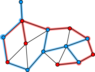
Figure 2: Illustration of Bicolored Noncrossing Spanning Trees problem. Note that we can use vertices of inline]KF: We have to reference this figure! inline]KF: We can think of whether drawing really a thick graph and within the thick graph our trees. opposite colors as a connector. Moreover, an edge may be used by both trees multiple times. We require, however, that the drawings of the spanning trees do not intersect.

Contrasting the result for one color, we show that our two-colored version of the spanning tree problem is NP-hard in plane graphs.

Theorem 1.4.

Bicolored Noncrossing Spanning Trees in plane linecolor=red,backgroundcolor=red!25,bordercolor=red,inline](Important Todo!)
KF: unweighted? graphs is NP-hard.

We complement our hardness result with a PTAS.

Theorem 1.5.

Bicolored Noncrossing Spanning Trees in plane unweighted graphs admits an $(1+\varepsilon)$-approximation scheme with $f(\varepsilon)n^{\mathcal{O}(1/\varepsilon)}$ running time for some function $f$.

We note that the trees are allowed to visit vertices of the other color. Thus, they can be also viewed as Steiner trees with the constraint that every Steiner point is a colored vertex. However, because of this constraint, Bicolored Noncrossing Spanning Trees is not a generalization of the Steiner tree problem in planar graphs and therefore its hardness status is not directly determined by that problem.

In the literature, only restricted variants of Bicolored Noncrossing Spanning Trees have been considered (without a bound on the number $k$ of colors, though): if there are at most two terminals per color, the problem can be solved in ${2^{\mathcal{O}(h^{2})}n\log k}$ time where $h$ is the number of face boundaries containing all terminals, and $n$ is the number of vertices [14]. If there are only constantly many terminals per color and all terminals lie on $h=2$ face boundaries, the problem is solvable even in ${\mathcal{O}(n\log n)}$ time [24]. On the plane, only a slightly different variant of the problem has been studied [21] where the spanning trees are not allowed to visit terminals of other colors. The authors obtained NP-hardness proofs and polynomial-time algorithms for various special cases but their results have not yet been formally published. There is also an approximation result for a noncrossing problem called colored spanning trees [13]. However, despite its name, this problem is a generalization of the Steiner tree problem allowing arbitrary Steiner points.

Noncrossing Paths

We also revisit the rather classic problem that we call Multicolored Noncrossing Paths. Given a set of linecolor=red,backgroundcolor=red!25,bordercolor=red,](Important Todo!)
KF: use the word terminal? We have to be consistent throughout the whole paper! terminal point pairs in the plane, the task is to connect each pair by a path such that the paths are pairwise noncrossing and their total length is minimized. One can think about this problem as an extension of our results to a large number of colors.

The best-known result is a randomized ${\mathcal{O}(\sqrt{n}\log n)}$-approximation algorithm by Chan et al. [9]. It is based on the heuristic by Liebling et al. [25] to connect the terminal pairs along a single tour through all the points. As a special case of the colored noncrossing Steiner forest problem, the problem also admits a (deterministic) $(1+\varepsilon)n/2$-approximation scheme [7].

The problem has been also studied in the presence of obstacle polygons whose boundaries contain all the terminal pairs. For the case of a single obstacle, Papadopoulou [31] gave a linear-time algorithm, whereas for the general case, Erickson and Nayyeri [14] obtained an algorithm exponential in the number of obstacles. A practical extension to thick paths has been considered by Polishchuk and Mitchell [33].

In this paper, we complement these algorithmic results and demonstrate that the problem is NP-hard.

Theorem 1.6.

Euclidean Multicolored Noncrossing Paths is NP-hard.

Thus, similar as Bicolored Noncrossing Spanning Trees in plane graphs, Multicolored Noncrossing Paths is a nice example of a problem whose hardness comes from the noncrossing constraint.

More Related Work

Very recently, Abrahamsen et al. [1] showed that the red-blue separation problem for geometric objects is polynomially time solvable (for two colors) if we allow any number of separating polygons and relax the connectivity requirement by allowing objects of the same color to lie in different regions. Interestingly, they showed that the red-blue-green separation problem for arbitrary objects remains NP-hard (for three colors) even if objects within each polygon do not need to stay connected.

We remark that the red-blue-green separation problem is related to the painter’s problem [17], where a rectangular grid and a set of colors $\chi=\{\text{red},\text{blue}\}$ is given. Each cell $s$ in the grid is assigned a subset of colors $\chi_{S}\subseteq\chi$ and should be partitioned such that, for each color $c\in\chi_{s}$, at least one piece in the cell is identified with $c$. The question is to decide if there is a partition of each cell in the grid such that the unions of the resulting red and blue pieces form two connected polygons. Van Goethem et al. [17] introduce a patching procedure that is similar to ours and used it to show that if the partition exists, then there exists one with a bounded complexity per cell. In a sense the problems are incomparable: in the red-blue-green separation problem a feasible solution always exists and the hard part is to find a minimum length solution. Additionally, our patching needs to be significantly more robust: we have to execute the patching procedure in portals (not in the whole cell) and our polygons can contain each other. Because of these technical issues, the number of crossings in our patching procedure is slightly higher (but it is still a constant).

Overview of the Paper

We start with a condensed overview of our techniques (Section 2) followed by a formal definition of our problems and a short preliminaries (Section 3). Then, in Section 4, we present our patching procedure which is a key ingredient to all our positive results: an EPTAS for Euclidean Bicolored Noncrossing Traveling Salesman Tours (Section 5) and for Euclidean Red-Blue-Green Separation (Section 6), and a PTAS for Bicolored Noncrossing Traveling Salesman Tours and Bicolored Noncrossing Spanning Trees, both in planar graphs (Section 7). At the end, we show NP-hardness of Bicolored Noncrossing Spanning Trees (Section 8) as well of Multicolored Noncrossing Paths (Section 9).

linecolor=red,backgroundcolor=red!50,bordercolor=red,inline](Important Question!)
KF: Maybe we should write about natural results that we didn’t obtain. (Plane versus graph results.). And about more colors (see SDOA rebuttal).

2 Our Techniques

Our algorithmic results are based on the plane dissection technique proposed by Arora [3]. In this framework, the space is recursively dissected into squares in order to determine a quadtree of $\mathcal{O}(\log(n/\varepsilon))$ levels. The idea is to look for the solution that traverses neighboring cells via preselected portals on the boundary of the cells of the quadtree. Arora [3] defines portals as a set of $\mathcal{O}(\log(n)/\varepsilon)$ equidistant points and uses dynamic programming to efficiently find a portal-respecting solution. He also shows that the expected cost of the portal respecting-solution is only $\varepsilon$ times longer than the optimum one. See Section 3 for a detailed introduction to this framework [3].

This technique will not allow us to get a near-linear running time. One approach to reduce the running time of Arora’s algorithm [3] is to use Euclidean spanners [34]. However, it is not clear how to ensure that our solution is noncrossing when we restrict ourselves to solutions that respect only the edges of the spanner. To overcome this obstacle, we use a recently developed sparsity-sensitive patching procedure [22]. Roughly speaking, this allows us to reduce the number of portals from $\mathcal{O}(\log(n)/\varepsilon)$ to $\mathcal{O}(1/\varepsilon^{2})$ many portals without a need for spanners.

The sparsity-sensitive patching procedure was designed explicitly to solve the Euclidean traveling salesman problem. We modify the procedure and show it can also be used for the red-blue-green separation problem. In Section 5, we show that the analysis behind sparsity-sensitive patching can be adapted to also work for the noncrossing (traveling salesman) tours problem. This is quite subtle and we need to resolve multiple technical issues. For example, even the initial perturbation step used in previous work [3, 22] needs to be modified as we cannot simply place the points of the same color in the same point. We need to snap to the grid in such a way, that after looking at the original positions of points, the solution is still noncrossing. We overcome all of these technical issues in Section 5.

Patching for noncrossing polygons

The main contribution of our work lies in the analysis. For example, in order to bound the number of states in our dynamic programming of our framework, we need to bound the number of times the portal respecting solution is intersecting the quadtree cells. Our insight is a novel patching technique that works for noncrossing polygons. Our Insight: Two noncrossing polygons can be modified (with low cost) in such a way that they cross the boundaries of a random quadtree only a constant number of times. Similarly to the patching scheme of Arora, our patching technique allows us to limit the number of times that two noncrossing polygons cross a boundary of the quadtree. However, our situation is significantly more complicated. We need to guarantee that, after the patching is done, the tours remain noncrossing and contain the same set of points as the original ones.

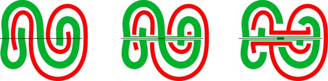
Figure 3: An example of our patching procedure for a case of disjoint objects that cross a horizontal line segment. The left figure presents the original objects (marked red and green). In the intermediate step, we patch the green object by possibly disconnecting the red object. Then we carefully cut the green object without disconnecting it to make “room” to reconnect the red object and guarantee connectivity. Note that the boundaries of the objects cross the horizontal segment only four times in the final picture. The whole construction is presented in Section 4

Now we briefly sketch the idea behind our patching scheme (see Section 4 for a rigorous proof and Figure 3 for a schematic overview). First, we apply several simplification rules to our polygons. We want to ensure that two colors are repeating consecutively in pairs. For example, in Figure 3, the borders of the green and the red polygon are pairwise intertwined in left-to-right order. Next, we introduce a split operation. After this operation is completed, the number of crossings is bounded, but it is not necessarily true that the polygons of the same color are connected (see the center of the Figure 3). At this point, the polygons form a laminar family. As the next step, we merge the polygons from the laminar families at so-called precise interfaces and combine them based on how the original polygons were connected. We refer the reader to Section 4 for a formal argument. In the end, we can bound the number of crossings by $10$.

Insight behind the lower bounds

Next, we describe our techniques behind the lower bounds. For brevity, we focus on the lower bound for Multicolored Noncrossing Paths. We reduce from Max-2SAT. Recall that the input to the problem is just a set of terminal points. We need these points to have some “rough structure” on top of which the paths from higher levels will bend. This inspires the idea to partition the terminals into four levels. These levels are needed to devise appropriate gadgets. We want to place the terminals in such a way that gadgets from higher levels do not interfere with gadgets from lower levels. The idea is to place terminal pairs from lower levels more densely than from the higher ones. This allows us to enforce the optimum solution to be exact on the pairs from level one. See Section 9 for a formal proof.

The NP-hardness proof of Bicolored Noncrossing Spanning Trees is more standard. We reduce from the Steiner tree problem and show that the vertices of the second tree can be used as Steiner vertices in the first tree. We include the proof for completeness in Section 8.

3 Preliminaries

linecolor=blue,backgroundcolor=blue!50,bordercolor=blue,inline](Reviewer’s Comment!)
"make it clear that a tour does not have to consist of straight line segments and not necessarily between sites. But we can assume that in some sense." linecolor=blue,backgroundcolor=blue!50,bordercolor=blue,inline](Reviewer’s Comment!)
define "open" in "open curves" (the endpoints belong to the curves but they are different) linecolor=blue,backgroundcolor=blue!50,bordercolor=blue,inline](Reviewer’s Comment!)
TODO? add info for planar graphs "(most easily described by rotation-system-based data structures like the quad-edge or DCEL that would allow to split the cycle of vertices and faces around a vertex where the color changes.)"? linecolor=blue,backgroundcolor=blue!50,bordercolor=blue,inline](Reviewer’s Comment!)
Shorten formal problem definition as intuition already given (but extend it for journal version)

linecolor=red,backgroundcolor=red!25,bordercolor=red,](Important Todo!)
KF: We should define “noncrossing” and to cross (also/only in Arora’s sense) We start by formally defining the setting of our problems and discussing technical subtleties and differences to related work; see Section 3. Then we review some known tools that we later use to prove our approximation schemes; see Section 3.1.

In the geometric setting, the input to our problem consists of $n$ points in $\mathbb{R}^{2}$, called terminals. Each terminal is colored with one of $k$ available colors. In the combinatorial setting, the input consists of an edge-weighted planar graph together with a planar embedding. Some of the vertices (called terminals) are colored with one of the $k$ colors.

Intuitively speaking, the goal in both settings is to draw pairwise-disjoint geometric graphs of minimum total length. Depending on the problem, either the graphs separate any two terminals of different colors (but not of the same color), or each graph connects all the terminals of one color. In the first case, we thus have $k-1$ graphs, in the second one, $k$ many. For the geometric setting, we consider the Euclidean length, whereas for the combinatorial setting, the length depends on the edge weights. Additionally, for the combinatorial setting, we require that the solution lies within the point set of a “thick” planar drawing of the input graph (realizing the embedding given in the input) with all Steiner points residing on the vertices.

Geometric Setting.

Before we define the goal for the geometric setting, we first precise what we mean by a feasible and an optimal solution. linecolor=blue,backgroundcolor=blue!50,bordercolor=blue,inline](Reviewer’s Comment!)
187-190: You don’t have conditions that require TSP to be tours. (e.g., 3 open curves could share an endpoint). You insist that TSP be connected; you also want that (and tour conditions) for each colored curve in RGB Separation. A solution consists of several drawings where each drawing is the point set of finitely many simple open curves in the plane where two curves may intersect only at their endpoints and where all the curves are connected together (that is, any two curves either share an endpoint or there is a third curve such that both are connected with it). Thus, a drawing can also contain closed curves built up by two or more open curves. The length of a drawing is the total Euclidean length of the curves it consists of. The length of a solution is the total length of its drawings. The (Euclidean) length of an object $\pi$ is denoted by $\mathrm{wt}(\pi)$. Instead of length, we also use the term cost.

For the $k$-Colored Points Polygonal Separation problem, a feasible solution consists of $k-1$ pairwise disjoint drawings where each drawing is a closed curve and where any two terminals of different colors are separated by at least one of the drawings, that is, any path connecting these two terminals contains (intersects) at least one point from the solution. In other words, the solution consists of $k-1$ closed curves that subdivide the plane into $k$ regions each one containing all the terminals of one of the $k$ colors. We examined the case for $k=3$ called the Red-Blue-Green Separation problem.

For all the other problems studied in this paper, a feasible solution consists of $k$ pairwise disjoint feasible drawings, one for each color. A drawing is feasible if it visits (intersects) all terminals of its color. For the Bicolored Noncrossing Traveling Salesman Tours problem, we additionally require that the feasible drawings are closed curves that we also call tours .

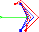
(a) A feasible solution.

(b) A cheaper feasible solution.

(c) An infeasible but noncrossing solution in the limit.

Figure 4: Three pairs of terminals (red disks, green crosses and blue squares) are connected via noncrossing paths. linecolor=blue,backgroundcolor=blue!50,bordercolor=blue,inline](Reviewer’s Comment!)
Fig 4 caption: identify the problem that this is illustrating (it is neither of the two just mentioned: Bicolored noncrossing TSP nor Red-Blue-Green Separation). The cycles->circles typo had me confused. In general, I like the biochemist convention that the caption should contain all the context needed to understand a figure. (See, e.g., https://journals.plos.org/ploscompbiol/article?id=10.1371/journal.pcbi.1003833 Rule 4.)

Informally, the goal is to find a solution of minimum length. However, note that for some input instances there does not exist a feasible solution of minimum length as there might be always a cheaper one obtained by drawing the curves closer to each other; see Fig. 4 for an example. In the limit, we obtain curves that may intersect, but that do not cross in the sense introduced by Arora [3]. In this sense, we define optimum solutions to be minimum-length solutions infinitesimally close to the limit (but still disjoint). However, for simplicity, we assume that the length of an optimum solution equals the length $\mathrm{OPT}$ in the limit. This assumption is also motivated by the known open problem whether it is possible to efficiently compute the Euclidean length of two sets of line segments up to a precision sufficient to distinguish their lengths.

Let us now formally define the goal of our $(1+\varepsilon)$-approximation schemes ( for constant $\varepsilon>0$) for the geometric setting in this paper. The goal is not to find a feasible almost-optimal solution but a so-called $(1+\varepsilon)$-cost-approximation.

Definition 3.1.

Let $X$ be a problem in our geometric setting and let $\mathcal{F}$ be the (possibly infinite) set of all feasible solutions to the problem. A number $x$ is a $(1+\varepsilon)$-cost-approximation of $X$ if

1. for every solution $S\in\mathcal{F}$, it holds that $x\leqslant(1+\varepsilon)\mathrm{wt}(S)$, and

2. there exists a solution $S^{\prime}\in\mathcal{F}$ such that $(1-\varepsilon)\mathrm{wt}(S^{\prime})\leqslant x$.

The two conditions guarantee that we return a number that is sufficiently close to the lengths of the cheapest feasible solutions (and thus to $\mathrm{OPT}$). The factor $(1-\varepsilon)$ in the second condition is only introduced to simplify our analysis: if there are two points in our solution that are infinitesimally close, we will count their distance to be $0$ (and therefore, in principle we may return a number $x$ that is smaller than $\mathrm{wt}(S)$ for every $S\in\mathcal{F}$). However, the second condition can be easily lifted to the more natural condition $\mathrm{wt}(S^{\prime})\leqslant X$ by multiplying $x$ by $1/(1-\varepsilon)$ and using a different constant in the first condition (on which $\varepsilon$ will depend).

Combinatorial Setting.

Next, we consider our problems in plane edge-weighted graphs. Formally, we fix any planar straight-line drawing of the given graph that realizes the given embedding. Without loss of generality, all vertices are drawn as closed discs with positive radius such that no two vertices intersect, and all edges have some positive width (in the sense of taking the Minkowski sum of the line segment corresponding to the edge and a disc of a sufficiently small radius). We require that an edge intersects only the vertices corresponding to its endpoints and no other edge. Terminals are drawn as points in the interior of their corresponding vertices.

A feasible solution is defined in the same way as in the geometric setting with one additional constraint. Namely, every curve is a straight-line segment drawn either within (i) the disc of a single vertex, or (ii) within a single edge and the discs of the edge’s endpoints such that the endpoints of the curve lie in opposite endpoints of the edge. If the curve lies within a vertex, we define its length to be $0$, otherwise its length is defined to be the weight of the corresponding edge.

In contrast to the geometric setting, there exist feasible solutions of minimum length $\mathrm{OPT}$ that we will call optimal solutions. Our goal is to compute the value $\mathrm{OPT}$. linecolor=red,backgroundcolor=red!50,bordercolor=red,](Important Question!)
KF: Right? Or do we compute an actual optimal solution?

Difference to Previous Definitions.

Note that our definition of a feasible solution slightly differs from the one in most previous works [14]. There the drawings of different colors are allowed to touch each other but must not cross in an intuitive sense. (Hence, such drawings are the limit case of our drawings when the length is locally minimal). The advantage of the previous definition is the existence of a minimum solution. The disadvantage is that crossings are formally defined via an untangling argument [14] which is hard to formally define and which essentially reduces to the statement that a solution is noncrossing if it can be made disjoint by an arbitrary small increase in the costs. Furthermore, the classical definition allows solutions with possibly undesirable properties; for example, a feasible solution can contain arbitrarily complicated networks of zero total length residing on a single point in the plane.

3.1 Useful Tools from Arora’s Approach

In this section, we describe the tools that Arora [3, 4] introduced to design his approximation scheme for geometric problems and that we further use in this paper. As defined above, the input of our geometric problems consists of a set $P$ of terminal points in $\mathbb{R}^{2}$ colored with some number of colors. It is fairly standard to preprocess the input points so that $P\subseteq\{0,\ldots,L\}^{2}$ for some integer $L=\Theta(n/\varepsilon)$ that is a power of $2$, even with the guarantee that points of different colors do not end up with the same coordinates. linecolor=red,backgroundcolor=red!25,bordercolor=red,inline](Important Todo!)
KF: $\varepsilon$ undefined. Define it in the beginning of the whole section?(We us it also in subsection 1.) For noncolored problems, such a peturbation costs only a $(1+\varepsilon)$ factor in the approximation ratio, but it is not obvious whether the bound holds also for multicolored problems due to the noncrossing constraint. Our contribution is to show the same cost bound for mutlicolored problems considered in this paper.linecolor=red,backgroundcolor=red!25,bordercolor=red,](Important Todo!)
KF: Mention this in our contribution in the introduction? Since the perturbation differs from problem to problem, we separately describe this preprocessing in detail in the respective sections.

A salesman path linecolor=red,backgroundcolor=red!25,bordercolor=red,](Important Todo!)
KF: But a path is not closed!? or a tour for a terminal set $P$ is a closed path that visits all points from $P$. Let us point out that in a tour the terminals are not necessarily connected with straight line segments. For a line segment $\mathrm{S}$ and a tour $\pi$, we let $\mathrm{I}(\pi,\mathrm{S})$ denote the (finite) set of points where $\pi$ crosses $\mathrm{S}$ (following Arora’s intuitive definition of crossing [3])linecolor=red,backgroundcolor=red!25,bordercolor=red,inline](Important Todo!)
KF: We should repeat Arora’s definition of noncrossing here (or even better: somewhere above) if we use it!. The set $\mathrm{I}(\pi,\mathrm{S})$ can also be interpreted as the set of intersection points of $\pi$ with $\mathrm{S}$linecolor=red,backgroundcolor=red!50,bordercolor=red,](Important Question!)
KF: But then we might have infinite many intersection points?, noting that infinitesimally close curves do not intersect. The following folklore lemma is typically used to reduce the number of times a tour crosses a given segment.

Lemma 3.2 (Patching Lemma [3, 4]).

Let $\mathrm{S}$ be a line segment and let $\pi$ be a simple closed curve. There exists a simple closed curve $\pi^{\prime}$ such that $|\mathrm{I}(\pi^{\prime},\mathrm{S})|\leqslant 2$ and $\mathrm{wt}(\pi^{\prime})\leqslant\mathrm{wt}(\pi)+3\cdot\mathrm{wt}(\mathrm{S})$. Moreover, $\pi$ and $\pi^{\prime}$ differ only within an infinitesimal neighborhood of $\mathrm{S}$.

Dissection and Quadtree.

Now we introduce a commonly used hierarchy to decompose (subspaces of) $\mathbb{R}^{2}$ that will be instrumental to guide our algorithm. Pick $a_{1},a_{2}\in\{1,\ldots,L\}$ independently and uniformly at random and define the random shift vector as $\mathbf{a}:=(a_{1},a_{2})$. Consider the square

$$C(\mathbf{a}):=[-a_{1}+1/2,\,2L-a_{1}+1/2]\times[-a_{2}+1/2,\,2L-a_{2}+1/2]$$

Note that $C(\mathbf{a})$ has side length $2L$ and each point from $P$ is contained in $C(\mathbf{a})$ by the assumption $P\subseteq\{0,\ldots,L\}^{2}$.

Let the dissection $D(\mathbf{a})$ of $C(\mathbf{a})$ be the tree $T$ that is recursively defined as follows. With each vertex of $T$, we associate an axis-aligned square in $\mathbb{R}^{2}$ that we call a cell of the dissection. For the root of $T$, this is $C(\mathbf{a})$. If a vertex $v$ of $T$ is associated with a square of unit length, we make it a leaf of $T$. Otherwise, $v$ has four children whose cells partition the cell of $v$. Formally, if $[l_{1},u_{1}]\times[l_{2},u_{2}]$ is the square associated with $v$, then each of its four children is associated with a different square $I_{1}\times I_{2}$ where $I_{i}$ is either $[l_{i},(l_{i}+u_{i})/2]$ or $[(l_{i}+u_{i})/2,u_{i}]$ for $i\in\{1,2\}$.

The quadtree $QT(P,\mathbf{a})$ is obtained from $D(\mathbf{a})$ by stopping the subdivision whenever a cell has at most one point from the input terminal set $P$. This way, every vertex is either a leaf whose cell (not necessarily a unit square) contains at most one terminal, or it is an internal vertex of the tree with four children whose cell contains at least two terminals.

Let $V(x)$ be the vertical line crossing the point $(x,0)$ and $H(y)$ be the horizontal line crossing the point $(0,y)$. A grid line is either a horizontal line $H(y)$ for $y=\frac{1}{2}+i$ where $i$ is integer, or a vertical line $V(x)$ for $x=\frac{1}{2}+i$ where $i$ is integer. For a line $\ell$ and a set $\mathcal{S}$ of line segments, we define $\mathrm{I}(\mathcal{S},\ell)$ as the set of all points through which the segments of $\mathcal{S}$ cross $\ell$. linecolor=red,backgroundcolor=red!25,bordercolor=red,](Important Todo!)
KF: We should either add that the segments are not parallel to $\ell$ (and then also update all lemmas using this notation, eg., Lemma 3.3) or that we use the definition of crossing of Arora and emphasize that in the case of infinite many intersections points, Arora’s definition allows to select a finite number of crossings points. Note that for every border edge $F$ of every cell in $D(\mathbf{a})$, there is a unique grid line that contains $F$. The following simple lemma relates the number of crossings between a set of line segments and the grid lines with the total length of the line segments; note that we assume that all endpoints are integer.

Lemma 3.3 ([28, Lemma 19.4.1]).

If $\mathcal{S}$ is a set of line segments in the a infinitesimal neighborhood of $\mathbb{Z}^{2}$, then

$$\sum_{\ell\text{ is a grid line}}|\mathrm{I}(\mathcal{S},\ell)|\leqslant\sqrt{2}\cdot\mathrm{wt}(\mathcal{S})~{}.$$

A portal is an infinitesimal short subsegment; in later sections, we define restricted type of solutions that cross the grid lines only through well-defined portals. For a segment $S$, we define $\mathrm{grid}(S,m)$ as the set of $m$ equispaced portals lying on $S$ (subsets of $S$) with the first and last portal lying infinitesimally close the endpoints of $S$ (thus, the distance between consecutive portals is bounded by $|S|/(m-1)$). linecolor=black,backgroundcolor=gray,bordercolor=black,]KF: In our proofs, $m$ is not necessarily integer.
Answer:We should say that we round it up. But recheck if $m$ is really not an integer. Maybe by our changes in the oter section, $m$ is always an integer now. linecolor=black,backgroundcolor=gray,bordercolor=black,]KF: 1) Neighboring boundaries share portals which causes extra care. 2) Patching a boundary might cause new crossings at another boundary.
Answer:Shift the first and last points such that they lie in the interior of the segment. See comment in other section why this helps. A border edge of a cell from $D(\mathbf{a})$ is called a boundary if there is no longer border edge on the grid line containing it. linecolor=red,backgroundcolor=red!25,bordercolor=red,](Important Todo!)
KF: Instead, make the border edges disjoint in the same flavor. We need the disjointness of the border edges for the DP. Due to a technical subtelty, we treat most boundaries as intervals that are open at one of their endpoints: if a point is contained in two boundaries, then we remove that point from the point set of the shorter of the two boundaries, or from an arbitrary one of the two if both have equal length; note that the removed point was always an endpoint of the affected boundary. If $F$ is a boundary, then its length is $2L/2^{i}$ for some integer $i$, and we define the level of the gridline containing $F$ as $i$. ( Gridlines not containing any boundaries, that is, not intersecting $C(\mathbf{a})$, have level $\infty$.) Intuitively, there are more grid lines with higher level than lower level; this fact is mirrored in the following lemma.

Lemma 3.4 ([28, Lemma 19.4.3]).

Let $\ell$ be a grid line and let $i$ be an integer satisfying ${0\leqslant i\leqslant 1+\log L}$. The probability that the level of $\ell$ is equal to $i$ is at most $2^{i}/L$.

4 Patching Procedure

linecolor=red,backgroundcolor=red!25,bordercolor=red,inline](Important Todo!)
KF: We need to extend the lemma in the sense, that (by the same costs), we can place the ten crossings points (in the given order) arbitrarily along the segment, or at least, that we can place all the ten crossing points on any given point of the segment (using Arora’s definition of noncrossingness). Alternatively, we could say that we place it infinitesimally close to any given point. Then we probably don’t need to use Arora’s definition. We just say, crossing at portals means, crossing in an infinitesimal neighborhood close to the portals. We could define infinitesimal by some arbitrary small function on the input size. AZP: I do not think there is time for drastic change of definitions.

linecolor=red,backgroundcolor=red!25,bordercolor=red,inline](Important Todo!)
KF: We should make it clear whether in this section we look at noncrossing solutions in Arora’s sense or in our disjoint sense. The order relation $<$ suggest that we mean our disjoint sense. Arora’s sense seems to appear only in context of portals. AZP: the idea was that if the curves touch, we just say that they are infinitesimal close to each other, but we consider them disjoint. The same with the curve and the segment - as long as they touch but do not cross we consider them disjoint but infinitesimally close. This implies that the crossing points are really the points and not the segments. I agree that this is sloppy but we inherit this sloppyness from Arora. In this section, we prove the following important generalization of Arora’s patching lemma [3, 4] (see Lemma 3.2 in Section 3) to noncrossing tours. The generalized patching lemma is a key ingredient for proving our approximation schemes for the Euclidean Bicolored Noncrossing Traveling Salesman Tours problem (Section 5) and the Euclidean Red-Blue-Green Separation problem (Section 6). It allows us to reduce the number of times that a tour crosses a cell of the quadtree.

Lemma 4.1 (Patching of noncrossing tours).

Let $\mathrm{S}$ be a line segment, and let $\pi_{\mathtt{R}}$ and $\pi_{\mathtt{B}}$ be two simple noncrossing closed curves. There exist two simple noncrossing curves $\pi^{\prime}_{\mathtt{R}}$ and $\pi^{\prime}_{\mathtt{B}}$ such that $|\mathrm{I}(\pi^{\prime}_{\mathtt{R}},\mathrm{S})\cup\mathrm{I}(\pi^{\prime}_{\mathtt{B}},\mathrm{S})|\leqslant 10$, and $\mathrm{wt}(\pi^{\prime}_{\mathtt{R}})+\mathrm{wt}(\pi^{\prime}_{\mathtt{B}})\leqslant\mathrm{wt}(\pi_{\mathtt{R}})+\mathrm{wt}(\pi_{\mathtt{B}})+20\cdot\mathrm{wt}(\mathrm{S})$ . Moreover, for $c\in\{\mathtt{R},\mathtt{B}\}$, $\pi_{c}$ and $\pi^{\prime}_{c}$ differ only within an infinitesimal neighborhood of $\mathrm{S}$. Furthermore, we can move all crossing points $\mathrm{I}(\pi^{\prime}_{\mathtt{R}},\mathrm{S})\cup\mathrm{I}(\pi^{\prime}_{\mathtt{B}},\mathrm{S})$ to any given portal through $\mathrm{S}$ by increasing the cost of $\pi^{\prime}_{\mathtt{R}}$ and $\pi^{\prime}_{\mathtt{B}}$ by only $\mathcal{O}(\mathrm{wt}(\mathrm{S}))$. linecolor=red,backgroundcolor=red!50,bordercolor=red,inline](Important Question!)
KF: Can we assume this without cost increase? AZP: probably some already resolved TODO.

linecolor=red,backgroundcolor=red!25,bordercolor=red,inline](Important Todo!)
KF: Say somewhere that if the input tour contains a subsegment of $\mathrm{S}$, then we can locally modify that segment without notable cost increase such that it crosses $\mathrm{S}$ only in one point. In sensitive patching, we might run in such situations, therefore we can’t just assume that this will not happen and thus this is important to write. AZP: we are actually assuming this does not happen by assuming infinitesimally close neighborhooods. If we want to explain it in more detail, we should do it when introducing the set I(S,tour). Right now we kind of just blame the confusion on Arora :)

For a simple curve $\pi$ that contains two points $y,z$, we define ${\pi}[{y},{z}]$ as the part of $\pi$ that goes from $y$ to $z$ and whose direction is counterclockwise in the case that $\pi$ is closed. For the purpose of this proof, we assume without loss of generality that $\mathrm{S}$ is aligned with the $x$-axis of the coordinate system. Let $\mathrm{I}(\pi_{\mathtt{R}},\mathrm{S})\cup\mathrm{I}(\pi_{\mathtt{B}},\mathrm{S})=\{x_{1},\ldots,x_{m}\}$ be the set of points in $\mathbb{R}^{2}$ through which $\pi_{\mathtt{R}}$ and $\pi_{\mathtt{B}}$ intersect $\mathrm{S}$ linecolor=red,backgroundcolor=red!25,bordercolor=red,inline](Important Todo!)
KF: What if they intersect with an segment, hence, have infinite many intersection points? We don’t disallow such cases. Before, we said that we look at crossings points, hence, in such cases such an intersection segment corresponds to a single crossing point. AZP: that is true, the intersection segment gives only one crossing point (if the curves really cross there). Again, it this is not clear, it should be explained when defining I(segment,tour). where $x_{1}<\dots<x_{m}$ is their order by the $x$-coordinate. Let $c(x_{i})=\mathtt{R}$ if $x_{i}$ is the intersection of $\mathrm{S}$ with $\pi_{\mathtt{R}}$ and $c(x_{i})=\mathtt{B}$ otherwise. We sometimes refer to $c(x_{i})$ as the color of $x_{i}$.

Claim 4.2.

For $1<i<m$, it holds that $x_{i}$ has a neighbor of the same color, that is, $c(x_{i+1})=c(x_{i})$ or $c(x_{i-1})=c(x_{i})$.

Proof.

Let us assume for the sake of contradiction that $c(x_{i})=\mathtt{R}$ and $c(x_{i+1})=c(x_{i-1})=\mathtt{B}$ (the case when $c(x_{i})=\mathtt{B}$ is symmetrical). The segment ${\mathrm{S}}[{x_{i-1}},{x_{i+1}}]$ and the curve ${\pi_{\mathtt{B}}}[{x_{i-1}},{x_{i+1}}]$ together form a closed curve that is crossed by $\pi_{\mathtt{R}}$ linecolor=red,backgroundcolor=red!25,bordercolor=red,](Important Todo!)
KF: by $\pi_{\mathtt{R}}$!?? exactly once. This is not possible because $\pi_{\mathtt{R}}$ linecolor=red,backgroundcolor=red!25,bordercolor=red,](Important Todo!)
KF: by $\pi_{\mathtt{R}}$!?? is also a closed curve. linecolor=blue,backgroundcolor=blue!50,bordercolor=blue,inline](Reviewer’s Comment!)
I though this was part of the proof of Lemma 4.1; since you refer to adjusting a single curve, I suspect you mean to refer to Aurora’s patching in Lemma (4?). AZP: Skipping this comment. linecolor=blue,backgroundcolor=blue!50,bordercolor=blue,inline](Reviewer’s Comment!)
"In many places there is too much detail (In an abstract, you don’t need to formally prove Claim 4.2, for example, just note that every other segment is inside one of the curves.)". AZP: skipping this comment. ∎

Simplification

We now group the intersection points $\{x_{1},\ldots x_{m}\}$ into maximal groups of consecutive monochromatic points. To be more precise, if $c(x_{i+1})=c(x_{i})$, then $x_{i+1}$ and $x_{i}$ are greedily selected to the same group. Let $H_{1},\ldots,H_{\ell}$ be the resulting (nonempty) groups and let $\mathrm{S}_{j}$, for $1\leqslant j\leqslant\ell$, be the segment spanning $H_{j}$. Without loss of generality, assume that the points of $H_{j}$ are colored $\mathtt{R}$ inline]KF: In this section we use $\mathtt{R}$ to refer to "red". Maybe we should (if not already) do the same consistently in other sections? for odd $j$ and colored $\mathtt{B}$ for even $j$. Observe that the segments in $\{\mathrm{S}_{j}\mid 1\leqslant j\leqslant\ell\}$ are pairwise disjoint. We now use the patching procedure of Arora (Lemma 3.2) inline,linecolor=lime,bordercolor=lime,backgroundcolor=lime!30]SODA Reviewer:
It would be helpful to state Lemma 5.1 of Arora. to modify the tours $\pi_{\mathtt{R}}$ and $\pi_{\mathtt{B}}$ into $\overline{\pi_{\mathtt{R}}}$ and $\overline{\pi_{\mathtt{B}}}$. To be more precise, we first modify the tour $\pi_{\mathtt{R}}$ by applying Lemma 3.2 independently to each segment $\mathrm{S}_{j}$ where $j$ is odd and $|H_{j}|>2$. Analogously, we modify the tour $\pi_{\mathtt{B}}$ on segments with even index. By Lemma 3.2, the tour $\overline{\pi_{\mathtt{R}}}$ intersects each segment $\mathrm{S}_{j}$ of odd $j$ at most twice (and at least once because the groups $H_{1},\dots,H_{\ell}$ are nonempty). Similarly, the tour $\overline{\pi_{\mathtt{B}}}$ intersects each even segment $\mathrm{S}_{j}$ at most twice. Moreover, $\mathrm{wt}(\overline{\pi_{c}})\leqslant\mathrm{wt}(\pi_{c})+3\cdot\mathrm{wt}(\mathrm{S})$ for $c\in\{\mathtt{R},\mathtt{B}\}$.

To summarize, we simplified our problem as follows. Let $\mathrm{I}(\overline{\pi_{\mathtt{R}}},\mathrm{S})\cup\mathrm{I}(\overline{\pi_{\mathtt{B}}},\mathrm{S})=\{y_{1},\ldots,y_{m^{\prime}}\}$ be the set of points in $\mathbb{R}^{2}$ through which $\overline{\pi_{\mathtt{R}}}$ and $\overline{\pi_{\mathtt{B}}}$ intersect $\mathrm{S}$ where $y_{1}<\ldots<y_{m^{\prime}}$ is their order by the $x$-coordinate. By the discussion above and by Claim 4.2, inline,linecolor=lime,bordercolor=lime,backgroundcolor=lime!30]SODA Reviewer:
Also, using this lemma [Lemma 5.1 of Arora.] the crossing is at most twice. In the next paragraph, how did it change to exactly two? It is correct but needs an explanation. the color sequence $c(y_{1}),\ldots,c(y_{m^{\prime}})$ does not contain any monochromatic triplets, and, with a possible exception of the first and last element, it consists of alternating pairs $\mathtt{R}\mathtt{R}$ and $\mathtt{B}\mathtt{B}$. In other words, $c(y_{1}),\ldots,c(y_{m^{\prime}})$ is an infix of a sufficiently long sequence $\mathtt{R},\!\mathtt{R},\,\mathtt{B},\!\mathtt{B},\ldots$ of alternating pairs. We continue the proof on this simplified instance.

Laminar and Parallel Tours

linecolor=red,backgroundcolor=red!50,bordercolor=red,inline](Important Question!)
KF: We never seem to directly use the properties of being laminar/parallel in the following proof.s (We only prove that something is laminar/parallel. But why are we proving it?) Observe that, essentially, there are only two different topologies that a pair of noncrossing tours can admit. We say that a tour $\sigma$ is parallel to linecolor=red,backgroundcolor=red!50,bordercolor=red,inline](Important Question!)
KF: Definition of laminar/parallel tours seems buggy: a pair of laminar tours is always also a pair of parallel tours: one tour lies always outside of the other one!! I think, we mean that two tours are parallel if each lies outside of the other one, and laminar, if one lies inside the other one!
If we define tours (not pairs) to be laminar/parallel with respect to some other tour, then the definition might work, but then we have also to define what we mean by a laminar/parallel pair of tours; see Fig. 6 a tour $\mu$ if $\mu$ lies outside of $\sigma$, otherwise $\sigma$ is laminar to $\mu$. linecolor=red,backgroundcolor=red!25,bordercolor=red,](Important Todo!)
KF: The segment $\mathrm{R}$ hasn’t been defined yet. It’s name is also confusing with the color $\mathtt{R}$! Do we mean $S$? AZP: I am removing the mention of R here. linecolor=blue,backgroundcolor=blue!50,bordercolor=blue,inline](Reviewer’s Comment!)
341: The segment R used here is not defined. You’ve used colors R,B for points above, and fig 6 uses S. (see below: 354: only now do we get the definition of R. ) For an illustration, see Fig. 6. linecolor=red,backgroundcolor=red!25,bordercolor=red,inline](Important Todo!)
KF: Instead of defining the property of laminar/parallel tours, we could make the following observations: AZP: if i understand correctly, we are leaving parallel laminar.
1) Each tour separates the plane into two parts, a finite inner part and an unbounded outer part.
2) When walking around the tour in counterclockwise direction, the inner part is thus always on the left-hand side.
3) We orient both tours in counterclockwise direction.
4) Any two neighboring passes of the same color (independently of whether there is another color in between(!)) must be oriented in opposite direction given 2) and 3) (either the inner or the outer part lies in between them).
5) Thus, the $i$-th and $j$-th pass (of the same color) are oriented in opposite direction if and only if $i$ and $j$ have different parity.
6) Thus, by connecting passes of different parity, we again obtain cycles.
7) Consequently, the splitting step is fully safe!
8) The merging step also as there we greedily connect passes of different parity, ensure that we have degree 2 everywhere, and that every color is connected. We must only argue that if and only if we can connect one color, we can also connect the other one. I think we can show this iff as follows: each split increases the number of red and blue components by one (above and below). Hence, after the split step, we have the same number of red and blue cycles. If we merge two blue cycles, then we also merge the two red cycles in between as they were disjoint before given the disjointness of the blue cycles. Thus, if we merge, then we decrease the number of blue and red components by one (above or below, respectively). Consequently, when we merged all blue cycles, we necessarily also merged all red cycles. Hence, we end up with exactly one blue and one red tour.

Split Operation

Next, we define the operation of splitting a pair of non-intersecting tours by a segment (for an intuitive illustration see Fig. 6). This operation is defined only for a segment that starts and ends in two distinct points of the first tour, intersects the second tour twice and has no other intersections with the two tours. To be more precise, let $\sigma$ and $\mu$ be two non-intersecting tours. Let $\mathrm{R}$ be a segment that connects two different points on $\sigma$ and intersects both $\mu$ and $\sigma$ exactly twice (so the intersections with $\sigma$ are precisely the endpoints of $\mathrm{R}$). For the purpose of this proof, the split operation will only be used for $\mathrm{R}$ being a subsegment of $\mathrm{S}$, but we define the split operation independently of $\mathrm{S}$.

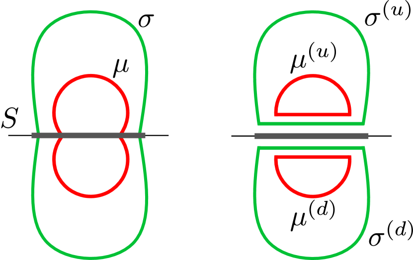
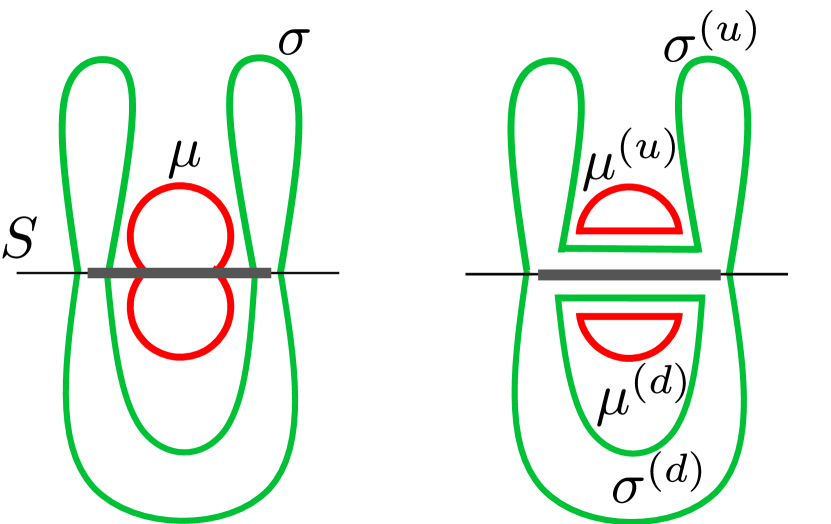
Figure 6: A schematic view of the splitting procedure for laminar (left figure) and parallel (right figure) tours. inline]KF: Inconsistency: in all figures we use green color whereas in the main text we write $B$ for blue. Since red-green blindness is the most common one (followed by blue-yellow), I suggest to use red and blue. inline]KF: Inconsistency2: In the figure we use $S$, in the text we use $R$. linecolor=red,backgroundcolor=red!25,bordercolor=red,inline](Important Todo!)
KF: Missing case (see main text): same crossing as in the first case, but red contains green. linecolor=blue,backgroundcolor=blue!50,bordercolor=blue,inline](Reviewer’s Comment!)
Ditto for fig 6 caption: define S and explain the lighter line. Define what distinguishes parallel and laminar.

linecolor=blue,backgroundcolor=blue!50,bordercolor=blue,inline](Reviewer’s Comment!)
Please use the notation of 356ff in Fig 6.

Let $p_{1},p_{2}$ be the intersection points of $\sigma$ with $\mathrm{R}$ (hence, the endpoints of $\mathrm{R}$) and let $q_{1},q_{2}$ be the intersection points of $\mu$ with $\mathrm{R}$. Without loss of generality, we assume that $\mathrm{R}$ is aligned with the $x$-axis and $p_{1}<q_{1}<q_{2}<p_{2}$ is the order of the points by the $x$-coordinate. Note that (excluding the endpoints) the segment $\mathrm{R}$ lies entirely inside of $\sigma$ if $\sigma$ is laminar to $\mu$, and entirely outside otherwise (see Fig. 6). We split $\sigma$ and $\mu$ as follows. We create two copies of $\mathrm{R}$, let us call them $\mathrm{R}^{(u)}$ and $\mathrm{R}^{(d)}$, inline,linecolor=lime,bordercolor=lime,backgroundcolor=lime!30]SODA Reviewer:
The notation $\sigma^{(u)}$ and $\sigma^{(d)}$ are a bit confusing, as they do not entirely lie in the up or down of S. and place them slightly above and slightly below $\mathrm{R}$ respectively. Next, we split $\sigma$ into two tours, $\sigma^{(u)}$ and $\sigma^{(d)}$, by first adding to $\sigma$ the two segments $\mathrm{R}^{(u)}$ and $\mathrm{R}^{(d)}$ and then removing the parts of $\sigma$ that connect the endpoints of linecolor=red,backgroundcolor=red!50,bordercolor=red,inline](Important Question!)
KF: But then we remove the tour completely as a cycle always has two parts connecting the same pair of points! (In our case the situation is even more complicated as we have several cycles after adding the two segments.) Formally, we could write that we first remove from $\sigma$ its four (or two if $\mathrm{R}$ is a point?) intersection points with $\mathrm{R}^{(u)}$ and $\mathrm{R}^{(d)}$, thus $\sigma$ consists of four open curves. Remove the two (?) curves that cross/intersect $\mathrm{R}$. Then close one of the remaining paths with $\mathrm{R}^{(u)}$, the other one with $\mathrm{R}^{(d)}$ to obtain $\sigma^{(u)}$ and $\sigma^{(d)}$. $\mathrm{R}^{(d)}$ with the endpoints of $\mathrm{R}^{(u)}$. Then, we create two copies of the segment $\mathrm{R}^{\prime}={\mathrm{R}}[{q_{1}},{q_{2}}]$, let us call them $\mathrm{R}^{\prime(u)}$ and $\mathrm{R}^{\prime(d)}$, and we place $\mathrm{R}^{\prime(u)}$ slightly above $\mathrm{R}^{(u)}$, and we place $\mathrm{R}^{\prime(d)}$ slightly below $\mathrm{R}^{(d)}$. We split $\mu$ with the segments $\mathrm{R}^{\prime(u)}$ and $\mathrm{R}^{\prime(d)}$ in an analogous way as we split $\sigma$. The split operation is presented in Fig. 6 for a laminar pair (left side) and for a parallel pair (right side).

As a result of a split operation we obtain two pairs of closed curves: above linecolor=red,backgroundcolor=red!25,bordercolor=red,](Important Todo!)
KF: But on the figure, $\sigma^{(u)}$ is everywhere (above and below) at the same time! We should state more precisely what we mean by above/below: that their endpoints are above/below. $\mathrm{R}$ we have a pair $\sigma^{(u)},\mu^{(u)}$, and below $\mathrm{R}$ we have a pair $\sigma^{(d)},\mu^{(d)}$. Observe that if the original tours were laminar, then both of these pairs are laminar and $\sigma^{(u)}$ is parallel to $\sigma^{(d)}$linecolor=red,backgroundcolor=red!25,bordercolor=red,](Important Todo!)
KF: Not true! we can redraw Fig. 6a) such that the red tour goes around the green one (but intersect $S$ as in the figure. After the split, $\sigma^{(u)}$ is NOT parallel to $\sigma^{(d)}$.. On the other hand, if the original tours were parallel, then one pair is parallel, the other is laminar and $\sigma^{(u)}$ is laminar to $\sigma^{(d)}$ (as in Fig. 6 ) or vice versa.

For both resulting pairs $(\sigma^{(a)},\mu^{(a)})$, $a\in\{u,d\}$, we refer to the pair of segments $(\mathrm{R}^{(a)},\mathrm{R}^{\prime(a)})$ as a precise interface of the pair $(\sigma^{(a)},\mu^{(a)})$, while the segment $\mathrm{R}$ is a rough interface of $(\sigma^{(a)},\mu^{(a)})$. Note that the precise interface is in a negligible distance to the corresponding rough interface. Also observe that $\mathrm{wt}(\sigma^{(u)})+\mathrm{wt}(\sigma^{(d)})+\mathrm{wt}(\mu^{(u)})+\mathrm{wt}(\mu^{(d)})\leqslant\mathrm{wt}(\sigma)+\mathrm{wt}(\mu)+4\mathrm{wt}(\mathrm{R})$.

Splitting $\overline{\pi_{\mathtt{R}}}$ and $\overline{\pi_{\mathtt{B}}}$

Our goal is to transform $\overline{\pi_{\mathtt{R}}}$ and $\overline{\pi_{\mathtt{B}}}$ as to make them intersect $\mathrm{S}$ at most ten times in total. Without loss of generality we assume that $\overline{\pi_{\mathtt{R}}}$ is either laminar to $\overline{\pi_{\mathtt{B}}}$ or it is parallel to $\overline{\pi_{\mathtt{B}}}$ (if neither is the caselinecolor=red,backgroundcolor=red!50,bordercolor=red,](Important Question!)
KF: Can it be neither case??, we swap the names of the two tours).

Let $\mathrm{R}_{1},\ldots,\mathrm{R}_{k}$ be segments that span all quadruples $y_{i},y_{i+1},y_{i+2},y_{i+3}\in\mathrm{S}$ such that $c(y_{i})=c(y_{i+3})=\mathtt{R}$ and $c(y_{i+1})=c(y_{i+2})=\mathtt{B}$ (see Fig. 7). We assume that $\mathrm{R}_{1}<\ldots<\mathrm{R}_{k}$ are ordered by the $x$-coordinates of their left endpoints. Observe that there are at most six intersections among $y_{1},\ldots,y_{m^{\prime}}$ which do not belong to the segments $\mathrm{R}_{1},\dots,\mathrm{R}_{k}$. As the first step of our transformation, we split the pair of tours $(\overline{\pi_{\mathtt{R}}},\overline{\pi_{\mathtt{B}}})$ with the segments $\mathrm{R}_{1},\ldots,\mathrm{R}_{k}$ one by one linecolor=red,backgroundcolor=red!25,bordercolor=red,inline](Important Todo!)
KF: It is not obvious that such a splitting will work. After each single split, we need to guarantee that we don’t come up with the situation that, for some unprocessed segment, two crossing points of the same color suddenly belong to different cycles. (Fig. 7 shows an example of $\overline{\pi_{\mathtt{R}}}$ and $\overline{\pi_{\mathtt{B}}}$ before and after the split). Let $\{(\sigma_{i},\mu_{i})\}_{i\in\{1,\ldots,k+1\}}$ be the set of pairs obtained after all splits are completed. linecolor=red,backgroundcolor=red!25,bordercolor=red,inline](Important Todo!)
KF: Given our mistakes above, I don’t have confidence that the following claims (until end of this paragraph) are correct. Maybe they are, but in any case we should prove them and not just write “Note that it holds.” Note that if $\overline{\pi_{\mathtt{R}}}$ is laminar to $\overline{\pi_{\mathtt{B}}}$, then, for every pair $(\sigma_{i},\mu_{i})$, the tour $\sigma_{i}$ is laminar to $\mu_{i}$ and, for $j\neq i$, parallel to $\sigma_{j}$. If, on the other hand, $\overline{\pi_{\mathtt{R}}}$ is parallel to $\overline{\pi_{\mathtt{B}}}$, then among the obtained pairs, there is precisely one pair $(\sigma_{j},\mu_{j})$ where $\sigma_{j}$ is parallel to $\mu_{j}$; hence, for $i\neq j$, the tour $\sigma_{i}$ is laminar to $\mu_{i}$. Moreover, for $i\neq j$, the tour $\sigma_{j}$ is laminar to $\sigma_{i}$ and, hence, also laminar to $\mu_{i}$.

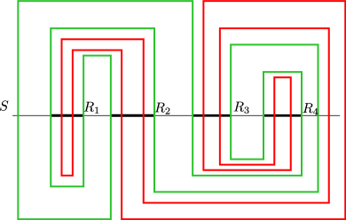
Figure 7: Before and after splittinginline]KF: Colors in figure inconsistent with definition: a quadruple should start/end in red and not in green (blue).inline]KF: Some labels too small, whereas some labels in some other figures are too big. In the ideal case, all labels should have over all figures have the same size as the main text.

Let $\overline{\mathrm{R}}$ be the minimum segment that contains all segments $\mathrm{R}_{i}$ for $i\in\{1,\ldots,k\}$. It is important to observe that, after the splitting, $\overline{\mathrm{R}}$ is not crossed by any of the tours. inline]KF: We should also argue about the total splitting cost somewhere as we refer to it at the final cost analysis.

Merging Precise Interfaces

From now on, the goal of the transformation is to merge the pairs resulting from the splitting in order to obtain again two tours in total.

To formally describe the process of merging, let us first define the operation of merging consecutive precise interfaces that both lie on the same side of the segment $\mathrm{S}$ (both above or both below). This operation is the reverse of splitting and it is illustrated in Fig. 8.

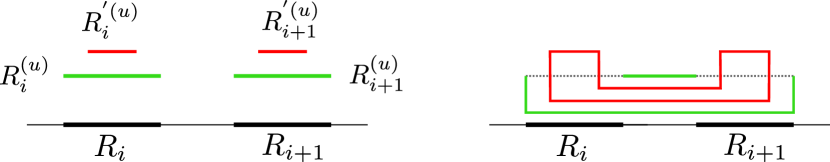
Figure 8: inline]KF: Labels way too big! inline]KF: We should make visually more clear where the precise interfaces are on the right side (e.g., by increasing the thickness of the dashed part and also replace the $R^{\prime}$s by the dashed part. The current variant of the figure wrongly suggests that the $R^{\prime}$s are still present and have not been remove; which is wrong. The thin red horizontal segments symbolize the red tour above the $R^{\prime}$s, but this is not clear). Merging two consecutive interfaces when the interfaces are above $\overline{\mathrm{R}}$. The left figure presents the interfaces before merging. The right procedure depicts the result after merging. The segments are removed and connected through the corridor inline]KF: depict the corridor as a gray shaded area? between them and inline]KF: not so clear what we mean. In the main text, there are two different types of corridors. $\overline{\mathrm{R}}$ in the noncrossing manner.

Let $(\mathrm{R}_{i}^{(a)},{\mathrm{R}^{\prime}}_{i}^{(a)})$, where $a\in\{u,d\}$, and $(\mathrm{R}_{i+1}^{(a)},\mathrm{R}_{i+1}^{\prime(a)})$ be two consecutive precise interfaces lying on the same side of $\mathrm{S}$. Let $(\sigma_{i}^{(a)},\mu_{i}^{(a)})$ and $(\sigma_{i+1}^{(a)},\mu_{i+1}^{(a)})$ be two distinct linecolor=red,backgroundcolor=red!50,bordercolor=red,](Important Question!)
KF: Can it happen that they are the same tours? Yes, it can! The word distinct wants to emphasize it, but this is not strong enough. It even wrongly suggests that the two pairs are always distinct. We should rephrase/add here something. And also, what do we do if the pairs are not distinct. We just keep and do not merge those precise interfaces? pairs of tours whose interfaces are $(\mathrm{R}_{i}^{(a)},\mathrm{R}_{i}^{\prime(a)})$ and $(\mathrm{R}_{i+1}^{(a)},\mathrm{R}_{i+1}^{\prime(a)})$, respectively. To merge the interfaces $(\mathrm{R}_{i}^{(a)},\mathrm{R}_{i}^{\prime(a)})$ and $(\mathrm{R}_{i+1}^{(a)},\mathrm{R}_{i+1}^{\prime(a)})$, we remove the segments $\mathrm{R}_{i}^{(a)}$, $\mathrm{R}_{i}^{\prime(a)}$, $\mathrm{R}_{i+1}^{(a)}$ and $\mathrm{R}_{i+1}^{\prime(a)}$ from the tours containing them. As a result, all four tours $\sigma_{i}^{(a)}$, $\mu_{i}^{(a)}$, $\sigma_{i+1}^{(a)}$ and $\mu_{i+1}^{(a)}$ become paths. We connect the endpoints of $\sigma_{i}^{(a)}$ with the endpoints of $\sigma_{i+1}^{(a)}$ linecolor=red,backgroundcolor=red!50,bordercolor=red,](Important Question!)
KF: Very unclear: which endpoints are connected together? $\sigma_{i}^{(a)}$ has two endpoints and $\sigma_{i+1}^{(a)}$ has two endpoints. in a noncrossing manner, and this creates a corridor very close to $\overline{\mathrm{R}}$. We then connect the endpoints of $\mu_{i}^{(a)}$ with the endpoints of $\mu_{i+1}^{(a)}$linecolor=red,backgroundcolor=red!50,bordercolor=red,](Important Question!)
KF: Again, which endpoints are precisely connected together?, in a noncrossing manner, via the corridor that was just created. This operation is depicted in Fig. 8. Thus, by merging precise interfaces, the associated pairs of tours are also merged into one pair $(\sigma^{(a)},\mu^{(a)})$. If both pairs that are merged are laminar, then observe that $\sigma^{(a)}$ is also laminar to $\mu^{(a)}$. If, on the other hand, one of the pairs is parallel, then the resulting pair is also parallel. linecolor=red,backgroundcolor=red!25,bordercolor=red,](Important Todo!)
KF: Check correctness of the claims concerning laminar/parallel!

Merging All Pairs

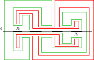
Figure 9: Our example after the transformation

We now describe the process of merging all pairs of the tours that were created during the splitting procedure. The idea is it to start, by merging pairs of tours whose precise interfaces lie above $\mathrm{S}$. Subsequently, we want to merge pairs of tours whose precise interfaces lie below $\mathrm{S}$. After this procedure, we may still obtain a constant number of distinct pairs of tours, one above and one below $\mathrm{S}$. In that case we merge them by crossing $\mathrm{S}$.

In more detail, we first iterate through the rough interfaces $\mathrm{R}_{2},\dots,\mathrm{R}_{k}$ (skipping $\mathrm{R}_{1}$). For each $\mathrm{R}_{i}$, we look at the pair $(\sigma^{(u)}_{i},\mu^{(u)}_{i})$ whose precise interface is $(\mathrm{R}_{i}^{(u)},\mathrm{R}_{i}^{\prime(u)})$. If $\sigma^{(u)}_{i}$ is not the same tour as $\sigma^{(u)}_{i-1}$linecolor=red,backgroundcolor=red!50,bordercolor=red,](Important Question!)
KF: But what if $\mu^{(u)}_{i}$ equals $\mu^{(u)}_{i+1}$, and what about the case that $\mu^{(u)}_{i}$ and $\mu^{(u)}_{i+1}$ differ but $\sigma^{(u)}_{i}$ and $\sigma^{(u)}_{i-1}$ not?, we merge the two precise interfaces $(\mathrm{R}_{i-1}^{(u)},\mathrm{R}_{i-1}^{\prime(u)})$ and $(\mathrm{R}_{i}^{(u)},\mathrm{R}_{i}^{\prime(u)})$linecolor=red,backgroundcolor=red!50,bordercolor=red,](Important Question!)
KF: What happens to their precise interfaces after the merge? They get destroyed, right? But then what happens to the sequence of the precise interfaces? Do we update it? Can it now happen that two precise interfaces become neighbors (consecutive) that weren’t consecutive before?. Thus, at the end, all the precise interfaces above $\mathrm{S}$ belong to the same pair of tours. In an analogous way, we proceed with the interfaces below $\mathrm{S}$ and obtain a single pair of tours below $\mathrm{S}$. If both pairs of tours, above and below $\mathrm{S}$, are the same, we are done. Otherwise, if the pairs are distinctlinecolor=red,backgroundcolor=red!50,bordercolor=red,](Important Question!)
KF: do we include the case that two tours from the pairs are the same while two others are distinct?, we merge the interface $(\mathrm{R}_{1}^{(u)},\mathrm{R}_{1}^{\prime(u)})$ with $(\mathrm{R}_{1}^{(d)},\mathrm{R}_{1}^{\prime(d)})$ which results in a single pair of tours crossing $\overline{\mathrm{R}}$ four times. For an example, see Fig. 8 that depicts the situation after merging the interfaces of Fig. 7. Note that merging all interfaces costs at most $8\mathrm{wt}(\mathrm{S})$linecolor=red,backgroundcolor=red!50,bordercolor=red,](Important Question!)
KF: Why factor $8$? Why a constant? Can’t it happen during the merging that repeatedly pairs of large distance that before were not consecutive, become consecutive (after pairs in between have been merged together and their precise interfaces got removed)?.

Summarized, the resulting tours $\pi^{\prime}_{\mathtt{R}}$ and $\pi^{\prime}_{\mathtt{B}}$ cross $\mathrm{S}$ at most ten times in total: at most six times linecolor=red,backgroundcolor=red!50,bordercolor=red,](Important Question!)
KF: Can we decrease it to four? (See comment in the beginning.) along $\mathrm{S}\setminus\overline{\mathrm{R}}$ as noted above, and at most four times along $\overline{\mathrm{R}}$ after the merging. Splitting the tours incurs an additional cost of at most $8\mathrm{wt}(\mathrm{S})$, while merging the tours also incurs an additional cost of at most $8\mathrm{wt}{\mathrm{S}}$. The initial transformation of Arora costs at most $3\mathrm{wt}(S)$. Thus, $\mathrm{wt}(\pi_{\mathtt{R}})+\mathrm{wt}(\pi_{\mathtt{B}})\leqslant\mathrm{wt}(\pi^{\prime}_{\mathtt{R}})+\mathrm{wt}(\pi^{\prime}_{\mathtt{B}})+20\mathrm{wt}(\mathrm{S})$ as promised.

5 Euclidean Bicolored Noncrossing Traveling Salesman Tours

In the following, we show that the problem of finding two noncrossing Euclidean traveling salesman tours, one for each color, admits an EPTAS.

See 1.3

In Section 5.1, we prove a helpful theorem that allows us to focus on restricted tours, which is a key ingredient for our PTAS in Section 5.2.

5.1 Our Structure Theorem

The structure theorem shows that tours obeying certain restrictions are not much more expensive than unrestricted ones. Kisfaludi-Bak et al. [22] called such restricted tours $r$-simple. Below, we extend this notion to our setting and introduce $r$-simple pairs of tours. We say that a pair of tours $(\pi_{1},\pi_{2})$ crosses a line segment $\mathrm{S}$ if $\pi_{1}$ crosses $\mathrm{S}$ or $\pi_{2}$ crosses $\mathrm{S}$. In this sense, we define $\mathrm{I}((\pi_{1},\pi_{2}),\mathrm{S})=\mathrm{I}(\pi_{1},\mathrm{S})\cup\mathrm{I}(\pi_{2},\mathrm{S})$ as the set of points at which the pair $(\pi_{1},\pi_{2})$ crosses $\mathrm{S}$.

Definition 5.1 ($r$-simple pair of tours).

Let $\mathbf{a}$ be a random shift vector. A pair of tours $(\pi_{1},\pi_{2})$ is $r$-simple if it is noncrossinginline]KF: defined to be noncrossing. remove noncrossing where we write r-simple. and, for any boundary $F$ of the dissection $D(\mathbf{a})$ crossed by the pair,

1. it crosses $F$ entirely through one or two portals belonging to $\mathrm{grid}(F,\lfloor r\log L\rfloor)$, or

2. it crosses $F$ entirely through portals belonging to $\mathrm{grid}(F,g)$, for $g\leqslant r^{2}/m$ where $m$ is the number of times $F$ is crossed.

Moreover, for any portal $p$ on a grid line $\ell$, the pair $(\pi_{1},\pi_{2})$ crosses $\ell$ at most ten times through $p$.

Our structure theorem is an extension of the structure theorem of Kisfaludi-Bak et al. [22] to noncrossing pairs of tours.

Theorem 5.2 (Structure Theorem).

Let $\mathbf{a}$ be a random shift vector, and let $(\pi_{1},\pi_{2})$ be a pair of noncrossing tours consisting only of line segments whose endpoints lie in an infinitesimal neighborhood of $\mathbb{Z}^{2}$. For any large enough integer $r$, there is an $r$-simple pair $(\pi^{\prime}_{1},\pi^{\prime}_{2})$ of noncrossing tours that differs from $(\pi_{1},\pi_{2})$ only in an infinitesimal neighborhood around the grid lines and that satisfies

$$\mathbb{E}_{\mathbf{a}}[\mathrm{wt}(\pi^{\prime}_{1}\cup\pi^{\prime}_{2})-\mathrm{wt}(\pi_{1}\cup\pi_{2})]=\mathcal{O}((\mathrm{wt}(\pi_{1})+\mathrm{wt}(\pi_{2}))/r)~{}.$$

In the remainder of this section, we prove Theorem 5.2. The proof is based on the sparsity-sensitive patching technique of Kisfaludi-Bak et al. [22] that we discuss here for completeness. The sparsity-sensitive patching transforms two noncrossing tours $\pi_{1},\pi_{2}$ into an $r$-simple pair $(\pi^{\prime}_{1},\pi_{2}^{\prime})$ of noncrossing tours by patching the tours along each boundary $F$ that does not satisfy the conditions of Definition 5.1. As shown later, by considering the boundaries one by one in non-increasing order of their length, the patching of one boundary will never affect the crossings of boundaries already considered; thus, in the end, all boundaries will satisfy the desired conditions.

Let $F$ be the boundary whose turn is now to be patched. Let $(\hat{\pi_{1}},\hat{\pi_{2}})$ be the pair of tours obtained from $(\pi_{1},\pi_{2})$ by the previous patching steps (initially, $(\hat{\pi_{1}},\hat{\pi_{2}})=(\pi_{1},\pi_{2})$). By choosing the $x$-axis parallel to $F$ and orienting it appropriately, we can assume that $F$ is horizontal with its open endpoint (if any) on the right side (in the direction of increasing $x$-coordinate). Inductively, we assume that $\mathrm{I}(({\pi_{1}},{\pi_{2}}),F)\subseteq\mathrm{I}((\hat{\pi_{1}},\hat{\pi_{2}}),F)$ and that the remaining crossing points, $H:=\mathrm{I}((\hat{\pi_{1}},\hat{\pi_{2}}),F)/\mathrm{I}(({\pi_{1}},{\pi_{2}}),F)$, lie together infinitesimally close to the right endpoint of $F$ and to the right of all the other crossing points. Let $i$ be the level of the grid line containing $F$.

First, we partition the crossings in $\mathrm{I}(({\pi_{1}},{\pi_{2}}),F)$ (thus, without $H$) into two sets $G$ and $N$. If their number, $k=|\mathrm{I}(({\pi_{1}},\pi_{{2}}),F)|$, is $0$, we set $G=\emptyset$ and $N=\emptyset$. Otherwise, let $c_{1}<\ldots<c_{k}$ denote their $x$-coordinates. The proximity of the $j$-th crossing $x$ in this set is defined as $\mathrm{pro}(x)=c_{j}-c_{j-1}$ (for $j=1$, use $c_{0}=-\infty$). We set $N$ as the set of all crossings in $\mathrm{I}(({\pi_{1}},{\pi_{2}}),F)$ with proximity at most $L/(2^{i}r)$, and $G$ as the set of the remaining crossings. If $|G|\leqslant 1$, we set $g=\lfloor r\log L\rfloor$, otherwise $g=\lfloor r^{2}/(10(|G|+1))\rfloor$.

Next, based on $N$, $G$ and $H$, we create a set $\mathcal{S}$ of disjoint line segments as follows: we connect each point in $N$ to its left neighbor, and each point in $G$ and all points in $H$ to their closest portals in $\mathrm{grid}(F,g)$. The union of all these connections yields a set, $\mathcal{S}$, of at most $|G|+1$ maximal segments (if not empty, the set $H$ is connected via an infinitesimally short segment, possibly belonging to a longer segment with points from $N$ and $G$).

Instead of using the standard patching procedure of Arora [3, 4] (Lemma 3.2), we apply Lemma 4.1 to each line segment of $\mathcal{S}$ to obtain a new pair of tours $(\hat{\pi}^{\prime}_{1},\hat{\pi}^{\prime}_{2})$ crossing $F$ at no more than $|G|+1$ portals and each portal at most ten times.

If $|G|\leqslant 1$, then we use at most two portals and they belong to $\mathrm{grid}(F,\lfloor r\log L\rfloor)$, which satisfies Case (a) of Definition 5.1. Otherwise, if $|G|>1$, observe that, $F$ is crossed $m\leqslant 10(|G|+1)$ times in total, which implies that $g=\lfloor r^{2}/(10(|G|+1))\rfloor$ satisfies the bound in Case (b) of Definition 5.1. Thus, we conclude with Lemma 4.1 that the resulting pair $(\hat{\pi}^{\prime}_{1},\hat{\pi}^{\prime}_{2})$ is noncrossing and satisfies the conditions of Definition 5.1 for the boundary $F$. Note that the new line segments that we introduced for patching may cross other boundaries (perpendicular to $F$) and thus introduce new crossing points on each of them infinitesimally close to $F$, that is, infinitesimally close to their respective open endpoints. Moreover, by our construction of the dissection, any affected boundaries are shorter and thus haven’t been considered yet by our patching procedure. Conversely, we can conclude that $(\hat{\pi}^{\prime}_{1},\hat{\pi}^{\prime}_{2})$ satisfies the conditions of Definition 5.1 also for any boundaries considered so far (whose length is equal or larger than $|F|$).

By Lemma 4.1, the total expected patching cost for $F$ (that is, $\mathrm{wt}(\hat{\pi}^{\prime}_{1}\cup\hat{\pi}^{\prime}_{2})-\mathrm{wt}(\hat{\pi_{1}}\cup\hat{\pi_{2}})$) is proportional to $\mathrm{wt}(\mathcal{S})$. Note that the attribution of $H$ is only infinitesimal to the total cost as all crossing points in $H$ are infinitesimally close to each other and readily lie on the last portal of $\mathrm{grid}(F,g)$ (furthermore, the cost can be charged to the patching cost of the boundary that caused the crossing points of $H$). Since $H$ has also no influence on the proximity of the other crossing points, we will bound the expected patching cost assuming that $H$ is empty; that is, in the following cost analysis, we assume $\mathrm{I}(\hat{\pi_{1}}\cup\hat{\pi_{2}})=\mathrm{I}({\pi_{1}}\cup{\pi_{2}})$. Following the analysis of Kisfaludi-Bak et al. [22], we first bound this cost for $F$ in terms of proximity. Subsequently, we show that each crossing point contributes in expectation $\mathcal{O}(1/r)$ to the total cost. This fact allows us to bound the total cost in terms of the number of crossing points and, finally, in terms of $\mathrm{wt}(\pi_{1})+\mathrm{wt}(\pi_{2})$.

To simplify the discussion, we overestimate the costs and charge every crossing point in $\mathrm{I}(({\pi_{1}},{\pi_{2}}),F)$ with the cost of being connected to the closest portal in $\mathrm{grid}(F,\lfloor r\log L\rfloor)$ (independently of wherwhere the point really is). Note that this grid corresponds to the portal placement of Arora [3, 4]. Thus, following Arora’s arguments [3, 4], this expected (amortized) charging cost amounts to $\mathcal{O}(1/r)$ for every crossing point and is thus within the desired bound (see above). For the case $|G|=1$, we are therefore left with bounding the total cost $\sum_{x\in N}\mathrm{pro}(x)$ of connecting the points in $N$ to their left neighbors. Since this sum is encompassed in a bound that we establish below for the case $|G|>1$, it will immediately follow that we can charge this sum with the expected value $\mathcal{O}(1/r)$ to each crossing point. Thus, from now on, we assume that $|G|>1$.

For each point in $G$, we pay no more than $|F|/(2(g-1))$ to connect it to its closest portal in $\mathrm{grid}(F,g)$. Since the definition of $G$ implies $|G|=\mathcal{O}(r)$, the total connection cost of the points in $G$ is bounded by

$$\sum_{x\in G}\frac{\mathrm{wt}(F)}{2(g-1)}=\mathcal{O}\left(\sum_{x\in G}\frac{L|G|}{2^{i}r^{2}}\right)=\mathcal{O}\left(\frac{L|G|^{2}}{2^{i}r^{2}}\right)~{}.$$ (1)

To further bound $|G|^{2}$ in terms of proximity, let $\rho$ denote the point in $G$ with the minimum $x$-coordinate. We apply Cauchy-Schwartz to the vectors $\big{(}\sqrt{\mathrm{pro}(x)}\big{)}_{x\in G\setminus\{\rho\}}$ and $\big{(}\sqrt{1/\mathrm{pro}(x)}\big{)}_{x\in G\setminus\{\rho\}}$, noting that $1/\mathrm{pro}(\rho)=0$ and $\sum_{x\in G\setminus\{\rho\}}\mathrm{pro}(x)\leqslant\mathrm{wt}(F)=2L/2^{i}$. Therefore, we have

$$|G\setminus\{\rho\}|^{2}\leqslant\left(\sum_{x\in G\setminus\{\rho\}}\mathrm{pro}(x)\right)\left(\sum_{x\in G}\frac{1}{\mathrm{pro}(x)}\right)\leqslant\frac{2L}{2^{i}}\sum_{x\in G}\frac{1}{\mathrm{pro}(x)}~{}.$$ (2)

Since $|G|^{2}\leqslant 4|G\setminus\{\rho\}|^{2}$ (as $|G|>1$), we can combine (2) with (1) and, altogether, obtain the bound

$$\mathrm{wt}(\mathcal{S})=\mathcal{O}\left(\sum_{x\in N}\mathrm{pro}(x)+\left(\frac{L}{2^{i}r}\right)^{2}\sum_{x\in G}\frac{1}{\mathrm{pro}(x)}\right)~{}.$$

(The right side also bounds the connection cost for $N$ of the case $|G|=1$.) Thus, each crossing point contributes a specific amount to the total bound depending on its proximity and the level $i$ of the grid line containing $F$. Recall that the proximity also depends on $i$ as the level determines whether a crossing point is the left-most one of its boundary and therefore whether its proximity is fixed to $\infty$. To remove this dependence on the level, we define, for each grid line $\ell$, the relaxed proximity of each crossing point $x\in\mathrm{I}((\pi_{1},\pi_{2}),\ell)$ as the distance to the left neighbor of $x$ in $\mathrm{I}((\pi_{1},\pi_{2}),\ell)$, and $\infty$ if there is no left neighbor. Thus, the relaxed proximity equals the old proximity for all but possibly the left-most point $\rho$ of $\mathrm{I}((\pi_{1},\pi_{2}),F)$. Similarly, let $N^{\prime}$ be the set of all crossing points in $\mathrm{I}((\pi_{1},\pi_{2}),F)$ with relaxed proximity at most $L/(2^{i}r)$ and let $G^{\prime}$ contain all the other points. Thus, either $N^{\prime}=N$ and $G^{\prime}=G$ (if $\mathrm{pro}^{\prime}(\rho)=\mathrm{pro}(\rho)$), or $N^{\prime}=N\cup\{\rho\}$ and $G^{\prime}=G\setminus\{\rho\}$. Using that $1/\mathrm{pro}(\rho)=0$, we have

$$\mathrm{wt}(\mathcal{S})=\mathcal{O}\left(\sum_{x\in N^{\prime}}\mathrm{pro}^{\prime}(x)+\left(\frac{L}{2^{i}r}\right)^{2}\sum_{x\in G^{\prime}}\frac{1}{\mathrm{pro}^{\prime}(x)}\right)~{}.$$

Note that $x\in N^{\prime}$ if and only if the level $i$ is at most $\theta(x):=\log(L/(r\cdot\mathrm{pro}^{\prime}(x)))$. Thus, the contribution of each crossing point $x$ to the total bound is $\alpha_{i}(x):=\mathcal{O}(\mathrm{pro}^{\prime}(x))$ if $i\leqslant\theta(x)$, and $\alpha_{i}(x):=\mathcal{O}\left((L/(2^{i}r))^{2}/\mathrm{pro}(x^{\prime})\right)$ otherwise.

Now, for a fixed grid line $\ell$ and a crossing point $x\in\mathrm{I}((\pi_{1},\pi_{2}),\ell)$, Lemma 3.4 allows us to bound the expected patching cost due to $x$ by

$$\sum_{i=0}^{1+\log L}\Pr[\ell\text{ has level }i]\cdot\alpha_{i}(x)=\mathcal{O}\left(\sum_{i=0}^{\theta(x)}\frac{2^{i}}{L}\mathrm{pro}^{\prime}(x)+\sum_{i=\theta(x)+1}^{1+\log L}\frac{L}{2^{i}}\frac{1}{r^{2}\mathrm{pro}^{\prime}(x)}\right)=\mathcal{O}\left(\frac{1}{r}\right)~{},$$

where the right side follows by the convergence of sums of geometric progressions. Consequently, the expected total patching cost along $\ell$ is bounded by $\mathcal{O}\left(|\mathrm{I}((\pi_{1},{\pi_{2}}),\ell)|/r\right)$. Adding everything up, the total expected patching cost along all grid lines is at most

$$\sum_{\ell}\mathcal{O}(|\mathrm{I}((\pi_{1},\pi_{2}),\ell)|/r) =\sum_{\ell}\mathcal{O}(|\mathrm{I}(\pi_{1}),\ell)|/r)+\sum_{\ell}\mathcal{O}(|\mathrm{I}(\pi_{2}),\ell)|/r)$$

$$=\mathcal{O}((\mathrm{wt}(\pi_{1})+\mathrm{wt}(\pi_{2}))/r)$$

by Lemma 3.3, as required.

5.2 EPTAS for Noncrossing Euclidean Tours

In this section, we are going to use our structure theorem to give an approximation algorithm for Bicolored Noncrossing Traveling Salesman Tours. For a fixed $\varepsilon>0$, our algorithm will provide a $(1+\varepsilon)$-approximation for this problem.

The input consists of two terminal sets $P_{1},P_{2}\subset\mathbb{R}^{2}$, each colored in a different color. A bounding box of a point set is the smallest axis-aligned square containing that set. If the bounding boxes of $P_{1}$ and $P_{2}$ are disjoint, then we can treat them as two independent (uncolored) instances of TSP and solve them using the algorithm of Kisfaludi-Bak et al. [22]. Thus, in the end, we assume that the two bounding boxes intersect. Let $L$ be the side length of the bounding box of $P_{1}\cup P_{2}$ and observe that $L\geqslant\mathrm{OPT}$. By scaling and translating the instance, we assume that $L$ is a power of $2$ and of order $\Theta(n/\varepsilon)$, and that the corners of the bounding box of $P_{1}\cup P_{2}$ are integer.

Perturbation

As mentioned in Section 3.1, we first perturb the instance such that all input terminals lie in $\{0,\ldots,L\}^{2}$ on disjoint positions. For this, we follow related work [3, 5, 7], and move every terminal in $P_{1}$ to the closest position in $\mathbb{Z}^{2}$ with even $x$-coordinate, and every terminal in $P_{2}$ to a closest position in $\mathbb{Z}^{2}$ with odd $x$-coordinate. Thus, no terminals of the same color end up in the same position. If there are terminals of the same color on the same position, we treat them from now on as a single terminal. Later, we argue that there is an optimum solution to this perturbed instance that is only negligibly more costly than an optimum solution to the original instance. From now on, we assume that $P_{1},P_{2}\in\{0,\ldots,L\}^{2}$.

Given $L$, the perturbed instance and a shift vector $\mathbf{a}$, we construct a quadtree $QT(P,\mathbf{a})$ as described in Section 3.1. Let $D(\mathbf{a})$ be the corresponding dissection. Our idea is to compute the cost of a noncrossing pair $(\pi^{\prime}_{1},\pi^{\prime}_{2})$ of tours that solves the perturbed instance optimally and that crosses each boundary of the dissection only through carefully selected portals. Later, we show that the solution is not much more expensive than the optimum solution to the original instance.

Each boundary of the dissection is allowed to be crossed only through portals belonging to a so-called fine portal set that we define as follows.

Definition 5.3.

Let $\mathbf{a}$ be a random shift vector. Set $B$ of portals is called fine for a boundary $F$ of $D(\mathbf{a})$ if

1. $|B\cap F|\leqslant 2$ and $B\cap F\subset\mathrm{grid}(F,\lfloor(\log L)/\varepsilon\rfloor)$, or

2. $B\cap F\subset\mathrm{grid}(F,1/(\varepsilon^{2}k))$ for some $k\geqslant|B\cap F|$.

Set $B$ of portals is called fine for a cell $C$ of the quadtree $QT(P,\mathbf{a})$ if $B$ is fine for each of the four boundaries of $D(\mathbf{a})$ that contain a border edge of $C$ and $B$ is contained in the union of the four boundaries. A set of paths (open nor closed) is called fine-portal-respecting if there is a portal set $B$ that is fine for each boundary and the tours cross each boundary only through the portals of $B$ and each portal at most ten times, and the paths are noncrossing.

Note that it is no coincidence that the definitions of fine-portal-respecting pairs of tours and $r$-simple pairs of tours are very similar. Indeed, later we observe that any $(1\/\varepsilon)$-simple pair of tours is fine-portal-respecting. Also, note that the conditions of the definition imply that a fine portal set has no more than $\mathcal{O}(1/\varepsilon)$ portals.

Now, our overall goal is to compute the cost of an optimum fine-portal-respecting pair of tours solving the perturbed instance. linecolor=red,backgroundcolor=red!25,bordercolor=red,](Important Todo!)
KF: Can we underestimate the cost as said in Section 3? The strategy is the same as in the standard approximation scheme for the traveling salesman problem [3]. We use the quadtree to guide our algorithm based on dynamic programming. Starting from the lowest levels of the quadtree, we compute partial solutions that we combine together to obtain solutions for the next higher levels. More concretely, for each cell of our quadtree, we define a set of subproblems, in each of which, we look for a collection of paths that connect neighboring cells in a prescribed manner while visiting all terminals inside. Depending on an input parameter of the subproblem, the paths of each color will be disjoint or form a cycle.

To define our subproblems, fix some cell $C$ and consider a fixed fine portal set $B$ for $C$. Let $\partial C$ be the set of border edges of $C$, and let $B^{\prime}=B\cap\partial C$. We want to guess how exactly each portal in $B^{\prime}$ is crossed by the fine-portal-respecting pair $(\pi^{\prime}_{1},\pi^{\prime}_{2})$ (recall that each portal can be crossed at most ten times according to Definition 5.3). For this reason, we define $V_{B^{\prime}}$ as a matrix of size $|B^{\prime}|\times 11$ all whose entries are numbers from the set $\{0,1,2\}$; thus, $V_{B^{\prime}}[b]$ is a vector of size $11$ and, for $b\in{B^{\prime}}$ and $i\in\{1,\ldots,11\}$, we have $V_{B^{\prime}}[b,i]\in\{0,1,2\}$. The interpretation of $V_{B^{\prime}}[b,i]$ is simple as follows. If $l_{b}$ is the minimum $i$ such that $V_{B^{\prime}}[b,i]=0$, then $l_{b}-1$ is the number of times the tours cross the portal $b$. For $i<l_{b}$, the value $V_{B^{\prime}}[b,i]$ determines whether the $i$-th crossing of $b$ is due to $\pi^{\prime}_{1}$ (value $1$) or due to $\pi^{\prime}_{2}$ (value $2$). Let $\mathrm{cpy}({B^{\prime}},V_{B^{\prime}})$ be a new set of colored portals, that is obtained by subdividing each portal $b\in{B^{\prime}}$ in $l_{b}$ shorter portals $b_{1},\dots,b_{l_{b}}$ (ordered along $F$ in a globally fixed direction), and by setting the color of $b_{i}$ to $c(b_{i})=V_{B^{\prime}}[b,i]$. For $j\in\{1,2\}$, let ${B^{\prime}}_{j}=\{b\in\mathrm{cpy}({B^{\prime}},V_{B^{\prime}}):c(b)=j\}$. The subproblem for the cell $C$ is additionally defined by two perfect matchings, $M_{1}$ on ${B^{\prime}}_{1}$ and $M_{2}$ on ${B^{\prime}}_{2}$ whose union is noncrossing. For $i\in\{1,2\}$, we say that a collection $\mathcal{P}$ of $|B^{\prime}_{i}|$ realizes $M_{i}$ if for each $(p,q)\in M_{i}$ there is a path $\pi_{i}\in\mathcal{P}$ with $p$ and $q$ as endpoints. The formal definition of a subproblem for a cell $C$ is as follows.

Noncrossing Multipath Problem Input: A nonempty cell $C$ of the quadtree, a fine portal set $B$ for $C$ with ${B^{\prime}}:=B\cap\partial C$, a matrix $V_{B^{\prime}}\in\{0,1,2\}^{|{B^{\prime}}|\times 11}$, and two perfect matchings, $M_{1}$ on ${B^{\prime}}_{1}=\{b\in\mathrm{cpy}({B^{\prime}},V_{B^{\prime}}):c(b)=1\}$, and $M_{2}$ on ${B^{\prime}}_{2}=\{b\in\mathrm{cpy}({B^{\prime}},V_{B^{\prime}}):c(b)=2\}$, such that $M_{1}\cup M_{2}$ is noncrossing, and a (possibly empty) subset $\mathrm{Cycle}$ of $\{1,2\}$. Task: Find two path collections $\mathcal{P}_{{B^{\prime}}_{1},M_{1}},\mathcal{P}_{{B^{\prime}}_{2},M_{2}}$ of minimum total length such that their union is fine-portal-respecting and that satisfy the following properties for all $i\in\{1,2\}$: • every terminal in $P_{i}\cap C$ is visited by a path from $\mathcal{P}_{{B^{\prime}}_{i},M_{i}}$, • the paths in $\mathcal{P}_{{B^{\prime}}_{i},M_{i}}$ are pairwise noncrossing and entirely contained in $C$, and • $\mathcal{P}_{{B^{\prime}}_{i},M_{i}}$ realizes the matching $M_{i}$ on ${B^{\prime}}_{i}$, and • if $i\in\mathrm{Cycle}$, then the paths in $\mathcal{P}_{{B^{\prime}}_{i},M_{i}}$ form a cycle and ${B^{\prime}}_{i}=\emptyset$.

Though our subproblems are similar to those used in approximation schemes for TSP in the literature [3, 22], there is one main difference: here, we have two types of paths that correspond to $\pi_{1}$ and $\pi_{2}$ in the solution. Exactly as in Arora’s approximation scheme [3], our dynamic programming fills a lookup table with the solution costs of all the multipath problem instances that arise in the quadtree. The details follow next.

Base Case

We start with the base case, where the cell $C$ is a leaf of the quadtree and contains at most one terminal. Without loss of generality, assume that if there is a terminal inside, then it is from $P_{1}$ (the algorithm for the other case is analogous). We will generate all subproblems for $C$ and solve each of them. Consider every fine portal set $B$ for $C$ and, for $B^{\prime}=B\cap\partial C$, every possible matrix $V_{B^{\prime}}$. Each matrix defines an instance $\mathrm{cpy}({B^{\prime}},V_{B^{\prime}})$ of at most $10|B|$ portals that are colored with $1$ and $2$. For each possible noncrossing pair of perfect matchings, $M_{1}$ on ${B^{\prime}}_{1}$ and $M_{2}$ on ${B^{\prime}}_{2}$, and each subset $\mathrm{Cycle}\subseteq\{1,2\}$ that is compatible with ${B^{\prime}}_{1}$ and ${B^{\prime}}_{2}$ (in the sense that if $i\in\mathrm{Cycle}$, then ${B^{\prime}_{i}}=\emptyset$) any path collection realizing $M_{i}$ can be connected in the portals together to a cycle without intersecting any other path collection realizing the other matching), we compute the cost of an optimum multipath solution. We use dynamic programming to enumerate all possible such pairs of perfect matchings together with their solutions. To be more precise, let us fix $B$ and $V_{B^{\prime}}$, then ${B^{\prime}}_{1}$ and ${B^{\prime}}_{2}$ are implied by the choice of $B$ and $V_{B^{\prime}}$. Let $p\in P_{1}$ be the only terminal inside $C$ (if it exists). We define $\mathtt{BaseCase}$ as our lookup table as follows. For every $X_{1}\subseteq{B^{\prime}}_{1}$, every $X_{2}\subseteq{B^{\prime}}_{2}$, and every set $X^{\prime}$ that contains a pair of elements from $X_{1}$ if $p$ exists, and is empty otherwise, the entry $\mathtt{BaseCase}[X_{1},X_{2},X^{\prime}]$ is a set containing every triple $(M_{1},M_{2},\mathrm{wt}(M_{1}\cup M_{2})$, where $M_{1}$ is a perfect matching on $X_{1}$ with $X^{\prime}\subseteq M_{1}$, $M_{2}$ a perfect matching on $X_{2}$, $M_{1}\cup M_{2}$ is noncrossing, and $\mathrm{wt}(M_{1}\cup M_{2})$ is the cost of a minimum path collection realizing the matchings within the cell where $p$ (if exists) is connected via the path realizing the pair in $X^{\prime}$. Initially, if $p$ does not exist, we set $\mathtt{BaseCase}[\emptyset,\emptyset,\emptyset]=\{(\emptyset,\emptyset,0)\}$. Otherwise, for every $a,b\in{B^{\prime}}_{1}$, we set $\mathtt{BaseCase}[\{a,b\},\emptyset,\{(a,b)\}]:=\{(\{(a,b)\},\emptyset,\mathrm{dist}(a,p)+\mathrm{dist}(p,b))\}$ (which intuitively means that $p$ is connected to the portals $a,b\in{B^{\prime}}_{1}$ and there are no other paths in $C$). We define a helpful operator to determine the cost of connecting a pair of portals: for $X^{\prime}\subseteq X_{1}$ defined as above and any pair of portals $(u,v)$ from ${B^{\prime}}_{1}$ or ${B^{\prime}}_{2}$, let $\mathrm{pathcost}(X^{\prime},(u,v)):=\mathrm{dist}(u,v)$ if $X^{\prime}$ is empty ($p$ does not exist) or, for $\{a,b\}=X^{\prime}$, the segment $uv$ does neither cross the segment $ap$ nor the segment $pb$; otherwise $\mathrm{pathcost}(X^{\prime},(u,v)):=\mathrm{dist}(u,p)+\mathrm{dist}(p,v)$. Next, for every $X_{1}\subseteq B_{1}$, $X_{2}\subseteq B_{2}$, $X^{\prime}\subseteq X_{1}$ with $|X^{\prime}|=2$ if $p$ exists, and $X^{\prime}=\emptyset$ otherwise, we compute $\mathtt{BaseCase}[X_{1},X_{2},X^{\prime}]$ with the following dynamic programming formula:

$$\mathtt{BaseCase}[X_{1},X_{2},X^{\prime}]:=\bigg{\{}~{}~{} \Big{(}M_{1}\cup\{(u,v)\},M_{2},\mathrm{wt}(M_{1}\cup M_{2})+\mathrm{pathcost}(X^{\prime},u,v)\Big{)}$$

$$\Big{|}~{} \{u,v\}\subseteq X_{1}\textrm{ and }$$

$$(M_{1},M_{2},\mathrm{wt}(M_{1}\cup M_{2}))\in\mathtt{BaseCase}[X_{1}\setminus\{u,v\},X_{2}]\text{ and }$$

$$(u,v)\text{ is noncrossing with }M_{1}\cup M_{2}~{}\bigg{\}}$$

$$\bigcup~{}$$

$$\bigg{\{}~{}~{} \Big{(}M_{1},M_{2}\cup\{(u,v)\},\mathrm{wt}(M_{1}\cup M_{2})+\mathrm{pathcost}(X^{\prime},u,v)\Big{)}$$

$$\Big{|}~{} \{u,v\}\subseteq X_{2}\textrm{ and }$$

$$(M_{1},M_{2},\mathrm{wt}(M_{1}\cup M_{2}))\in\mathtt{BaseCase}[X_{1},X_{2}\setminus\{u,v\}]\text{ and }$$

$$(u,v)\text{ is noncrossing with }M_{1}\cup M_{2}~{}\bigg{\}}$$

linecolor=red,backgroundcolor=red!25,bordercolor=red,inline](Important Todo!)
KF: This is the place to note that our computed cost is not the actual cost of a feasible solution but we should argue why we are arbitrarily close to it. Note that if $1\in\mathrm{Cycle}$ and $p$ exists, then we assume that $p$ is visited by an inifitesimal short cycle of length $0$. For fixed $B$ and $V_{B^{\prime}}$, this algorithm runs in $\mathcal{O}(2^{\mathcal{O}(|B|)})$ and computes the set of all perfect matchings and the corresponding partial solution costs (cf. the PTAS of Bereg et al. [7] to see how the base case is handled).

Algorithm

To enumerate and solve all subproblems of a non-leaf cell $C$, we enumerate all compatible subproblems of its four children $C_{1},\ldots,C_{4}$ in the quadtree, lookup their solutions and combine them to the implied subproblem for $C$. We do it as follows. For $i\in\{1,\dots,4\}$, we iterate over every possible fine set $B_{i}$ for $C_{i}$ and set ${B^{\prime}}_{i}=B_{i}\cap\partial C_{i}$, over every corresponding matrix $V_{{B^{\prime}}_{i}}$. For each such pair $B_{i},V_{{B^{\prime}}_{i}}$, we iterate through all pairs of matchings $M^{(i)}_{1}$ and $M^{(i)}_{2}$, and every subset $\mathrm{Cycle}_{i}\subseteq\{1,2\}$. For every such obtained quadruple $\left((B_{i},V_{{B^{\prime}}_{i}},M^{(i)}_{1},M^{(i)}_{2},\mathrm{Cycle}_{i})\right)_{i\in\{1,\dots,4\}}$ (each consisting of four quintuples), we first check whether $B_{1}\cup B_{2}\cup B_{3}\cup B_{4}$ restricted to the four boundaries around $C$ implies a fine set $B$ for $C$, whether $V_{{B^{\prime}}_{1}},\dots,V_{{B^{\prime}}_{4}}$ imply, for $B^{\prime}=B\cap\partial C$, a consistent matrix $V_{{B^{\prime}}}$, and whether the portals, matchings and $\mathrm{Cycle}_{1},\dots,\mathrm{Cycle}_{4}$ are compatible. By compatible, we mean that (i) for every border edge shared by two neighboring cells (among $\{C_{1},\dots,C_{4}\}$), both cells define exactly the same portals of the same color, (ii) $\mathrm{Cycle}_{1},\dots,\mathrm{Cycle}_{4}$ are pairwise disjoint and if $c\in\Cup_{i=1}^{4}\mathrm{Cycle}_{i}$, then there are no portals of color $c$ on $\partial C_{1},\dots,\partial C_{4}$, and (iii) for each color $c\in\{1,2\}$, the graph in which the portals of color $c$ are vertices and the matchings are edges is either a cycle or contains no cycles at all. The last point implies that $\mathrm{Cycle}$ for $C$ contains not only all colors from $\Cup_{i=1}^{4}\mathrm{Cycle}_{i}$ but also all colors for which the graph was a cycle. Next, if the above conditions hold, we join the matchings by contracting degree two vertices in the graphs above. For graphs that were no cycles, this operation results in (new) matchings with endpoints on $\partial C$ in the portals $\mathrm{cpy}(B^{\prime},V_{{B^{\prime}}})$. Finally, if the resulting perfect matchings $M_{1}$ and $M_{2}$ are noncrossing, we obtained a complete description of a subproblem for $C$. We sum up the solutions costs of the respective subproblems of the four children and store them in our lookup table if this cost is the best found so far for this subproblem for $c$.

For every quadruple $\left((B_{i},V_{{B^{\prime}}_{i}},M^{(i)}_{1},M^{(i)}_{2})\right)_{i\in\{1,\dots,4\}},\mathrm{Cycle}_{i}$, it takes time polynomial in $1/\varepsilon$ to check whether it defines a valid subproblem for $C$ (and to compute a solution to it).

After completing the lookup table, our algorithm returns the cost for any subproblem for the root cell of the quadtree with $\mathrm{Cycle}=\{1,2\}$.

Analysis

Next, we show that this algorithm runs in $2^{\mathcal{O}(1/\varepsilon)}n\,\textup{polylog}(n)$ time. For each boundary, if we want to place a set of $k$ portals, we have $\binom{\mathcal{O}((\log L)/\varepsilon)}{k}=\binom{\mathcal{O}((\log n)/\varepsilon)}{k}$ possibilities in Case (a) of Definition 5.3 (assuming $k\leqslant 2$), and, for every feasible $k^{\prime}\geqslant k$ such that $k\leqslant 1/(\varepsilon^{2}k^{\prime})$, we have $\binom{\frac{1}{\varepsilon^{2}k^{\prime}}}{k}$ possibilities in Case (b). Thus, for every cell, the number of possible fine portal sets is

$$\left(\sum_{k=0}^{2}\binom{\mathcal{O}((\log n)/\varepsilon)}{2}+\sum_{2\leqslant k\leqslant k^{\prime}\textrm{ s.t. }k\leqslant 1/(\varepsilon^{2}k^{\prime})}\binom{\frac{1}{\varepsilon^{2}k^{\prime}}}{k}\right)^{4}=2^{\mathcal{O}(1/\varepsilon)}\,\textup{polylog}(n)~{},$$

using $\sum_{2\leqslant k\leqslant k^{\prime}\textrm{ s.t. }k\leqslant 1/(\varepsilon^{2}k^{\prime})}\binom{\frac{1}{\varepsilon^{2}k^{\prime}}}{k}=2^{\mathcal{O}(1/\varepsilon)}$ (see Claim 3.4 by Kisfaludi-Bak et al. [22]). Note that the number of possible noncrossing matchings on $k$ fine portals is known to be bounded by the $k$-th Catalan number whose value is of order of $\mathcal{O}(2^{k})$. Since $k\leqslant 1/\varepsilon$ (as noted above) and given that the number of cells in the quadtree is $\mathcal{O}(n\log n)$, we conclude that the number of states in our dynamic programming algorithm is bounded by $2^{\mathcal{O}(1/\varepsilon)}n\,\textup{polylog}(n)$. Observe that to get one level up in the dynamic programming, we combine the solutions computed for the children by iterating through all the states of the children cells. This iteration takes $2^{\mathcal{O}(1/\varepsilon)}\,\textup{polylog}(n)$ time as there are $2^{\mathcal{O}(1/\varepsilon)}\,\textup{polylog}(n)$ states for each child and it takes time polynomial in $1/\varepsilon$ to check if the states are compatible.

Finally, we analyze the approximation ratio of our algorithm. Assume that $\pi_{1},\pi_{2}$ is an optimal solution of cost $\mathrm{OPT}$. First, we argue that snapping points to $\mathbb{Z}^{2}$ perturbs the solution by at most $\mathcal{O}(\varepsilon\cdot\mathrm{OPT})$. Consider a point $p\in P_{1}$ (the case when $p\in P_{2}$ is analogous) that got perturbed. Let $c$ be the position to which $p$ is moved. We are going to add a segment $cp$ and $pc$ (infinitesimally close to each other) to the curve $\pi_{1}$ in order to guarantee that the point $p$ is visited after the perturbation. This, however, may cause that $\pi_{2}$ becomes intersected. To avoid that, we are going to use Lemma 4.1 on both curves to guarantee that segment $cp$ is crossed $O(1)$ times by the curve $\pi_{2}$. We route all these crossing points around $cp$ in $O(1)$ “layers”. This patching increases the total lengths of the curves by $\mathcal{O}(|cp|)$ which is bounded by $O(1)$. Since there are only $\mathcal{O}(n)$ nonempty cells, the snapping to the grid increases the cost of the solution by at most $\mathcal{O}(n)=\mathcal{O}(\varepsilon L)=\mathcal{O}(\varepsilon\mathrm{OPT})$.

Thus, there exists a solution of cost $\mathrm{OPT}+\mathcal{O}(\varepsilon\mathrm{OPT})$ to the perturbed instance. Without loss of generality, we can assume that it consists only of line segments with all endpoints lying in an infinitesimal neighborhood around the terminals. Since the terminals have integer coordinates, we can apply Theorem 5.2 for $r=1/\varepsilon$ and obtain a new solution $\pi_{1}^{A}$ and $\pi_{2}^{A}$ that (i) is $1/\varepsilon$-simple, and (ii) of length bounded by $\mathrm{OPT}+\mathcal{O}(\varepsilon\mathrm{OPT})$.

We claim that this solution is also fine-portal-respecting. If $(\pi_{1}^{A},\pi_{2}^{A})$ uses $u$ portals on a boundary $F$ from $\mathrm{grid}(F,g)$, then we set $k=r^{2}/g$ (recall $r=1/\varepsilon$) in Case (b) of Definition 5.3 and obtain exactly the same grid for our fine portals. It remains to observe $k\geqslant u$ as required by the definition. Since $u$ is not larger than the number $m$ of times $F$ is crossed, Definition 5.1 implies $g\leqslant r^{2}/m\leqslant r^{2}/u$ and therefore $k=r^{2}/g\geqslant r^{2}\cdot u/r^{2}=u$.

Finally, recall that our algorithm computes the cost of an optimum fine-portal-respecting pair of tours. By the discussion above this cost is bounded by $\mathrm{wt}(\pi_{1}^{A})+\mathrm{wt}(\pi_{2}^{A})=\mathrm{OPT}+\mathcal{O}(\varepsilon\mathrm{OPT})$ which concludes the proof of Theorem 1.2.

It is easy to see that the algorithm can be derandomized by trying all possibilities for $\mathbf{a}$ (but the cost increases by a polynomial in $n$ factor).

6 Red-Blue-Green Separation

inline]KF: The problem has been already defined; thus we should remove this paragraph or rephrase it in the style “Recall that …” We present an EPTAS for the Euclidean Red-Blue-Green Separation problem. In this problem, we are given three sets of different points $R,G,B\subseteq\mathbb{R}^{2}$linecolor=yellow,backgroundcolor=yellow!8,bordercolor=yellow,](Just a note for us)
KF: $\mathbb{R}$ is correct as only in the perturbed instances we have integer coordinates. The input is in reals.. We say that points in $R$ are “red”, points in $G$ are “green” and points in $B$ are “blue”. We desire two simple noncrossing polygons $P_{1}$ and $P_{2}$ of smallest total length such that all classes of points are separated by them, that is, for any two points $p_{i}$ and $p_{j}$ of different color, any path from $p_{i}$ to $p_{j}$ must cross $P_{1}$ or $P_{2}$.

linecolor=red,backgroundcolor=red!50,bordercolor=red,inline](Important Question!)
KF: Shouldn’t this part be moved to the introduction? Is it even not already there? The problem is NP-hard. To the best of our knowledge, only a special case of twolinecolor=black,backgroundcolor=gray,bordercolor=black,]KF: What "two"? two-colored
Answer:Yes. red-blue separation has been previously considered. For the red-blue separation problem, Mata and Mitchell [27] gave an $\mathcal{O}(\log n)$-approximation algorithm. Later, Arora and Chang [5] presented a PTAS for the red-blue separation problem.

Our contribution is twofold. First, we generalize the result of Arora and Chan [5] to three colors. Second, we give an EPTAS with $2^{\mathcal{O}(1/\varepsilon)}n\,\textup{polylog}(n)$ running time.

See 1.1

Now, we discuss the innovations that enabled us to generalize the result of Arora and Chang [5]. Their algorithm is based on the quadtree framework that was introduced to give a PTAS for Euclidean TSP. We replace it with a more efficient sparsity-sensitive patching already introduced in Section 5. Apart from minor modifications, this framework and the proof of the existence of an EPTAS is almost exactly the same as in Section 5. The main innovation is the introduction of a new patching procedure that allows us to extend the result of Arora and Chang [5] to three colors. In the next subsection, we analyze the red-blue-separation problem with the sparsity-sensitive patching framework. Next we will show our patching procedure for three colors.

6.1 EPTAS for Red-Blue-Green Separation

As a first step, we guess a topology of the optimum solution. We need to guess whether one of the polygons is fully contained within the other or whether they are separated. Moreover we need to guess a color of the points contained within each polygon. Without loss of generality, let us assume that $P_{1}\setminus P_{2}$ contains red points and $P_{2}\setminus P_{1}$ contains green points. Our algorithm consists of several steps that replicate the steps from Section 5 (and mostly from [5]).

Perturbation

This step is analogous to the perturbation step introduced in [5] and the goal is to guarantee three properties: each point has integral coordinate, the maximum internode distance is $\mathcal{O}(n/\varepsilon)$ and the distance between each pair of points is at least $8$. The perturbation procedure described in [5] places a grid of small granularity on the instance and moves each point to the closest grid point. To separate points of the same color we move red points to the closest north-east grid point $g_{r}$ with $x(g_{r})\equiv 1\;(\text{mod }4)$, blue to north-west grid point $g_{b}$ with $x(g_{b})\equiv 2\;(\text{mod }4)$ and green points to the closest south east grid point $g_{g}$ with $x(g_{g})\equiv 3\;(\text{mod }4)$. Later, we argue that the optimum solution to this perturbed instance is only negligibly more costly than the solution to original instance.

Arora and Chang [5] define the red bounding box as a linecolor=red,backgroundcolor=red!50,bordercolor=red,](Important Question!)
KF: the smallest axis-aligned? square of length $L_{r}$ that contains all the red points such that the red bounding box contains any polygon that separates red and blue points. They need to consider it to have a lower bound on optimum, because it could be the case that blue points are spread very far from red points. Because we assume that $P_{1}$ contains all the red points and $P_{2}$ contains all the green points we need to also define green bounding box of side-length $L_{g}$ that contains all green points. Observe, that if green-bounding-box does not intersect red-bounding-box then we can assume that we are given two independent dent instances of instance with two colors (and use $L_{r}$ and $L_{g}$ as a lowerbounds on $\mathrm{OPT}$ in these instances). On the other hand, if red and green bounding boxes intersect, we have a lower-bound $\mathrm{OPT}>\min\{L_{r},L_{g}\}$ and we can use $L=\min\{L_{r},L_{g}\}$ to lower-bound the $\mathrm{OPT}$ and determine the granularity (see [5] for details).

Next, in the step 2 we construct a randomly shifted quadtree. This step is identical to the quadtree construction in Section 5 (note that no input point lies on a boundary of a quadtree after this procedure). We draw a random $1\leqslant a_{1},a_{2}\leqslant L$ and create a dissection $D(a_{1},a_{2})$.

Structure theorem

Our structure theorem here is completely analogous to the structure theorem introduced in Section 5.2. linecolor=red,backgroundcolor=red!25,bordercolor=red,inline](Important Todo!)
KF: Rephrase definition to make it consistent with new definiton for TSP.

Definition 6.1 ($r$-simple pair of polygons).

Let $\mathbf{a}$ be a random shift vector. A pair of polygons $(P_{1},P_{2})$ is $r$-simple if it is noncrossing and, for any boundary $F$ of the dissection $D(\mathbf{a})$ crossed by the pair $(\partial P_{1},\partial P_{2})$,

1. it crosses $F$ entirely through one or two portals belonging to $\mathrm{grid}(F,\lfloor r\log L\rfloor)$, or

2. it crosses $F$ entirely through portals belonging to $\mathrm{grid}(F,g)$, for $g\leqslant r^{2}/m$ where $m$ is the number of times $F$ is crossed.

Moreover, for any portal $p$ on a grid line $\ell$, the pair $(\partial P_{1},\partial P_{2})$ crosses $\ell$ at most ten times through $p$.

Theorem 6.2 (Structure Theorem).

Let $\mathbf{a}$ be a random shift vector, and let $(P_{1},P_{2})$ be a pair of simple noncrossing polygons consisting only of line segments whose endpoints lie in an infinitesimal neighborhood of $\mathbb{Z}^{2}$. For any large enough integer $r$, there is an $r$-simple pair $(\hat{P}_{1},\hat{P}_{2})$ of noncrossing simple polygons whose borders that differ from $(\partial P_{1},\partial P_{2})$ only in an infinitesimal neighborhood around the grid lines and that satisfies

$$\mathbb{E}_{\mathbf{a}}[\mathrm{wt}(\partial\hat{P}_{1})+\mathrm{wt}(\partial\hat{P}_{2})-\mathrm{wt}(\partial P_{1})-\mathrm{wt}(\partial P_{2})]=\mathcal{O}((\mathrm{wt}(\partial P_{1})+\mathrm{wt}(\partial P_{2}))/r).$$

Moreover if $(P_{1},P_{2})$ are separating points $R,G,B$ then so are $(\hat{P}_{1},\hat{P}_{2})$.

The proof of Theorem 6.2 follows the framework used in the Theorem 5.2.

Dynamic Programming

Now we are going to briefly sketch the dynamic programming assuming Theorem 6.2. The dynamic programming will enable us to exactly find two $\mathcal{O}(1/\varepsilon)$-simple and noncrossing polygons in the given quadtree. This fact combined with the properties of Theorem 6.2 will guarantee that these polygons are $(1+\varepsilon)$ approximation.

At a high level, the states of the dynamic programming are very similar to ones defined in Section 5.2. The subproblems of the dynamic programming are defined as follows:

Separating $s$-simple polygons Input: A nonempty cell $C$ in the shifted quadtree, a fine portal set $B\subseteq\partial C$, a matrix $V_{B}$, and (ii) two perfect noncrossing matchings $M_{1},M_{2}$ on $B_{1}=\{b\in\mathrm{cpy}(B,V_{B}):c(b)=1\}$ and $B_{2}=\{b\in\mathrm{cpy}(B,V_{B}):c(b)=2\}$ respectively (iii) a $3$-coloring which indicates whether each region defined by matchings $M_{1}$ and $M_{2}$ is inside $P_{1}\setminus P_{2}$, inside $P_{2}\setminus P_{1}$ or neither Task: Find two $r$-simple path collections $\mathcal{P}_{B_{1},M_{1}},\mathcal{P}_{B_{2},M_{2}}$ of minimum total length that satisfies the following properties for all $i\in\{1,2\}$ • All points of class $R$ (respectively $G,B$) in cell $C$ are inside the region colored $R$ (respectively $G,B$), • Paths of $\mathcal{P}_{B_{i},M_{i}}$ are entirely contained in cell $C$ • $\mathcal{P}_{B_{i},M_{i}}$ realizes the matching $M_{i}$ on $B_{i}$.

The size of the lookup table is the number of subproblems. Number of possible colourings (iii) for a fixed matchings and portals is $2^{\mathcal{O}(1/\varepsilon)}$. We showed in Section 5.2 that the number of fine sets $B$, the corresponding matrices $V_{B}$ and non-crossing matchings $M_{1}$ and $M_{2}$ ((i) and (ii)) is $2^{\mathcal{O}(1/\varepsilon)}n\,\textup{polylog}(n)$. Thus, the total number of states for the dynamic programming here is also $2^{\mathcal{O}(1/\varepsilon)}n\,\textup{polylog}(n)$.

Each subproblem is solved by combining the previous one in the usual bottom-up manner. For a fixed state in the quadtree cell we iterate through all the solutions in 4 children in the quadtree. For each tuple we check if selected portals match, if corresponding matchings are connected and whether coloring across cell is consistent. If so, we remember the one with the smallest total length. linecolor=red,backgroundcolor=red!25,bordercolor=red,](Important Todo!)
KF: Analogous to my comment in TSP section, each subproblem should, for each color, also store the information whether it fully contains the polygon of that color.

It remains to describe the base case (which is analogous to the dynamic programming procedure described in Section 5.2). For a quadtree with a single node. Recall that all the input vertices are infinitesimally close to the corner of the cell. If the cell is empty, the solution is valid if the pairs of connected portals can be connected with a noncrossing matching. If the cell contains single point, we need to check that the region selected in the state matches the color of the point. Otherwise, our polytopes may need to “bend”linecolor=red,backgroundcolor=red!50,bordercolor=red,](Important Question!)
KF: And how do we compute the correct bend in polynomial time? on the points in order to separate the region. Observe that if the points of different colour have distance linecolor=red,backgroundcolor=red!50,bordercolor=red,](Important Question!)
KF: How can this happen? By perturbation (and alone, our assumption of the base case), we have at most one terminal in the cell! $0$, then all we need to do is make polygon go through it.

Now we argue that this procedure returns a $(1+\varepsilon)$ approximation to the original problem. During a perturbation step we shifted the points of the different colors to the different corners of the grid of granularity $\mathcal{O}(\varepsilon\mathrm{OPT}/n)$. Consider a point $p$ inside a grid cell $C$. Let $c\in C$ be the corner of the grid towards which the point $p$ is moved to by a snapping procedure. We add to optimum solution to the original instance the segments $cp$ and $pc$. This ensures that point $p$ is inside a proper polygon. Note, that this may create an additional crossings. To avoid that, we use Lemma 4.1 on segment $cp$. This guarantees that there exist two noncrossing polygons that does cross segment $pc$ only on point $c$. This operation increases the lengths of $P_{1}$ and $P_{2}$ by at most $\mathcal{O}(|pc|)$. In total this is bounded by the side-length of the grid which is $\mathcal{O}(\varepsilon\mathrm{OPT}/n)$. There are at most $\mathcal{O}(n)$ cells on which we do this operation. Hence after perturbation the length increases by at most $\mathcal{O}(\varepsilon\mathrm{OPT})$.

The analysis of the approximation factor due to the dynamic programming follows analogously to the analysis in Section 5.

7 Approximation Schemes in Planar Graphs

In this section, we complement our results, and demonstrate that our new patching lemma (Lemma 4.1) gives approximation algorithms in planar graphs.

See 1.3

We use a framework proposed by Grigni et al. [18] that enabled them to give a PTAS for TSP in planar graphs. Grigni et al. [18] proposed the following binary decomposition tree $\mathcal{T}$ of planar graph $G$. The decomposition is parametrized with $f,d\in\mathbb{N}$ that intuitively control approximation and depth of decomposition. Each node of $\mathcal{T}$ contains a subgraph of $G$. At the root of $\mathcal{T}$ is $G$ itself. For each node $H\in\mathcal{T}$, there exist $\mathcal{O}(f)$ vertex disjoint paths in $H$ (we call these paths portal paths). Removal of this paths partitions $H$ into $H_{1}$ and $H_{2}$, such that $H_{1},H_{2}\subseteq H$, and $|H_{1}|,|H_{2}|<\frac{5}{6}|H|$. These subgraphs $H_{1},H_{2}$ are then put recursively as two children of $H$ in the decomposition $\mathcal{T}$. The construction continues until at the leaves of $\mathcal{T}$ are subgraphs of size $s=\mathcal{O}(f^{2})$. The depth of tree $\mathcal{T}$ is $d$ and the total length of all portal paths in $\mathcal{T}$ is $\mathcal{O}(\frac{d}{f}|G|)$ (see Fig. 10 for one step of decomposition).

Figure 10: Figure depicts the graph $H$ as a node in a decomposition of Grigni et al. [18]. We have three portal paths (drawn in red) for a balanced planar separator that partitions graph $H$ into $H_{1}$ (drawn in blue) and graph $H_{2}$. The graph is recursively decomposed until subgraph is of size $s$. The patching lemma is applied on portal-paths to guarantee that solution is crossing $H_{1}$ and $H_{2}$ few times.

Lemma 7.1 (cf, [18]).

Given a planar graph $G$, in polynomial time one can compute a decomposition $\mathcal{T}$ with the following properties parameters $f:=\Theta((\log n)/\varepsilon)$ and $d:=\Theta(\log n)$. inline]KF: Write the time more accurately, say polynomial in what parameter(s)? That $\varepsilon$ treated as a constant?

We build an approximate solution to Bicolored Noncrossing Traveling Salesman Tours with a dynamic programming in the similar fashion as [18]. For a sake of presentation let us focus For each graph $H\in\mathcal{T}$ and information about connectivity of cycles we store a partial solution in the dynamic programming table. More precisely, each entry of dynamic programming contains a following states: (i) a current node $H$ from $\mathcal{T}$, (ii) set $\mathcal{P}$ of at most $\mathcal{O}(f)$ portal paths in $H$, (iii) set $\mathcal{C}(H,\mathcal{P})$ of configurations on portal paths in node $H$ that intuitively stores the information about the connectivity of the solution and how it looks “outside” $H$. More precisely, in $\mathcal{C}(H,\mathcal{P})$ we store a set of $\mathcal{O}(|\mathcal{P}|)$ “noncrossing pairings” between portal paths. Each pairing has either blue or red color and is connecting exactly two portal paths. Additionally, a single portal path can be a part of at most $\mathcal{O}(1)$ pairings. Moreover, pairing can be represented as the planar graph (i.e., pairings are noncrossing).

Remark.

The description of the subproblem is exactly the same as in Section 5, however we cannot artificially increase the number of portals (hence each portal would need to be a part of $\mathcal{O}(1)$ number of portals).

To solve the problem, we build our dynamic table bottom up. We start with the description of base case.

Base Case

Let $H$ be a leaf of $\mathcal{T}$. Based on the planar separator theorem, we give an $(1+\varepsilon)$-approximation algorithm in $f(\varepsilon)\cdot 2^{\mathcal{O}(\sqrt{|H|})}$ time to solve base case. On the input, we are given a set $\mathcal{P}$ of portal paths and a information about the connectivity $\mathcal{C}(H,\mathcal{P})$ between them. First, we compute a balanced separator of $H$ of size $\mathcal{O}(\sqrt{H})$ [26]. For each vertex on the separator, we guess how many times the cycle of each color is crossing it. By Lemma 4.1, we have a guarantee that there exists a feasible solution that crosses each vertex at most $\mathcal{O}(1)$ times. After that, we recurs into subgraphs determined by the planar separators until the size of the graphs is $\mathcal{O}(1/\varepsilon)$ (where we use an exhaustive algorithm in $f(\varepsilon)$ time). The running time is:

$$T(|H|)=2^{\mathcal{O}(\sqrt{|H|})}\cdot T(2|H|/3)\leqslant f(\varepsilon)2^{\mathcal{O}(\sqrt{|H|})}.$$

We need to analyse the approximation factor of our algorithm. Observe, that on a single call our patching cost is $\mathcal{O}(\sqrt{H})$, because we use Lemma 4.1 to bound number of crossings of vertices on the separator. Therefore, the approximation ratio is $E(|H|)=\mathcal{O}(\sqrt{|H|})+2T(2|H|/3)$ and $E(1/\varepsilon)=0$. This recursive equation results in the cost $E(|H|)=\mathcal{O}(\varepsilon|H|)$, which concludes the correctness of the base case.

Combination of Subproblems

We combine two solutions from the lower levels of $\mathcal{T}$ by checking if the states are compatible and selecting the solution of the lowest cost. We define the states to be compatible as in Section 5. For the running time, it is enough to compute the number of states in the dynamic programming table. The main contribution comes from the number of possibilities for $\mathcal{C}(H,\mathcal{P})$. Note, that the number of noncrossing pairings is $2^{\mathcal{O}(|\mathcal{P}|)}\leqslant n^{\mathcal{O}(1/\varepsilon)}$ (because each pairing can be represented as noncrossing matching on $\mathcal{O}(|\mathcal{P}|)$ vertices). This matches the runtime of the computation of the base case.

Approximation Ratio

It remains to bound the approximation cost. The approximation error comes with the assumption that our solution is crossing each portal path $\mathcal{O}(1)$ number of times and with solving each base case. For the base case error observe that the total size of each leaves in $\mathcal{T}$ is $(1+\mathcal{O}(1/\varepsilon))n$ and in the base case we incur $\mathcal{O}(\varepsilon)$ error per vertex. Therefore, we are left to analyse the approximation incurred by invoking patching lemma. Observe, that Lemma 4.1 given an optimum tour $\pi$, guarantees that there exists a tour $\pi^{\prime}$ that crosses each portal path $\mathcal{O}(1)$ and the cost of $\pi^{\prime}$ is only constant times longer than the total length of all portal paths. The decomposition lemma (see Lemma 7.1) guarantees that the total length of portal paths is $\mathcal{O}(\varepsilon n)$. Because optimum is at least $n/2$, we can select constant in front of $\varepsilon$ to guarantee $(1+\varepsilon)$ approximation. This concludes the correctness of our algorithm.

Remark.

Essentially, the same arguments can be used to give a polynomial time approximation scheme for Bicolored Noncrossing Spanning Trees linecolor=black,backgroundcolor=gray,bordercolor=black,]KF: in planar graphs, right?
Answer:Yes, and add this info everywhere where it is missing.. The main difference is that we need to use a significantly simpler patching Lemma for two colored trees of Bereg et al. [7] that allows additional Steiner vertices in portals.

See 1.5

8 NP-hardness of Bicolored Noncrossing Spanning Trees

In this section we consider the following problem.

Bicolored Noncrossing Spanning Trees

INPUT: a plane graph $G$ and a bipartition $(B,R)$ of $V(G)$, and an integer $k$.

PROBLEM: Are there two noncrossing trees $\mathcal{T}_{B}$ and $\mathcal{T}_{R}$ such that $\mathcal{T}_{B}$ spans $B$, $\mathcal{T}_{R}$ spans $R$ and $||\mathcal{T}_{B}||+||\mathcal{T}_{R}||\leqslant k$.

See 1.4

Proof.

The problem is in NP, since given the trees as a witness, it is easy to check that they form a solution. Let us show that it is NP-hard.

We reduce from (Unweighted) Steiner Tree in planar graphs [16]. Consider an instance of Steiner Tree, that is a graph $G$, a set $P$ of vertices called terminals, and an integer $k$. We can assume that $G$ is connected.

Consider a planar embedding of $G$ in the Euclidean plane. Let $G^{\prime}$ be the graph obtained from $G$ by subdividing every edge once. One can easily get an embedding of $G^{\prime}$ by adding the new vertices anywhere on their edges (besides their endpoints).

Let $f$ be a face of $G$ of degree $d$, and $C_{f}$ be the closed curve bounding $f$. Let $C^{\prime}_{f}$ be a cycle obtained from $C_{f}$ as follows:

1. Choose a point in $C_{f}$ that is not a vertex. Follow the curve $C_{f}$, and every time you encounter a vertex, add a new copy of that vertex. Let $v_{1}$, …, $v_{d}$ be the vertices created this way, in this order.

2. For $i\in\{1,\ldots,d-1\}$, let $v_{i}v_{i+1}$ be an edge. Also let $v_{1}v_{d}$ be an edge.

3. For $i\in\{1,\ldots,d\}$, add one edge connecting $v_{i}$ to the vertex of $C_{f}$ it was created as the copy of.

Note that for any face $f$, $C^{\prime}_{f}$ can be embedded inside $f$.

Let $G^{\prime\prime}$ be the graph $G^{\prime}$ such that, for every face $f$ of $G^{\prime}$, the cycle $C^{\prime}_{f}$ is added to the graph. Note that $G^{\prime\prime}$ is still a planar graph. Note that every vertex of $G^{\prime}$ of degree $d$ has exactly $d$ copies in $G^{\prime\prime}$. Let $B=P$ and $R=V(G^{\prime\prime})\setminus P$. Let $\ell=2k+|G^{\prime\prime}|-|P|-1$. This concludes the description of our reduction.

Correctness

Let us show that $(G,P,k)$ is a yes-instance to Steiner Tree if and only if $(G^{\prime\prime},B,R,\ell)$ is a yes-instance to Bicolored Noncrossing Spanning Trees.

Suppose that $(G,P,k)$ is a yes-instance to Steiner Tree. Let $\mathcal{T}$ be a Steiner tree of size $k$ in $(G,P)$. Let $\mathcal{T}^{\prime}$ be $\mathcal{T}$ with every edge subdivided once in $G^{\prime}$. Note that $\mathcal{T}^{\prime}$ is a tree using only vertices of $G^{\prime}$ spanning $B=P$ in $G^{\prime\prime}$.

Consider the dual $G^{\star}$ of $G$, and a spanning tree $\mathcal{S}$ of $G^{\star}$ that does not intersect $\mathcal{T}$. Let us build a tree $\mathcal{S}^{\prime}$ in $G^{\prime\prime}$ as follows:

1. Let $V(\mathcal{S}^{\prime})=R$

2. For every face $f$ of $G^{\prime}$ of degree $d$, for $i\in\{1,\ldots,d-1\}$, add $v_{i}v_{i+1}$ to $\mathcal{S}^{\prime}$.

3. For every edge $e$ of $\mathcal{S}$, let $u_{e}$ be the vertex of $G^{\prime}$ subdividing the dual edge of $e$ in $G$, and let $u_{e}^{\prime}$ and $u_{e}^{\prime\prime}$ be the two copies of $u_{e}$ in $G^{\prime\prime}$. Add $u_{e}u_{e}^{\prime}$ and $u_{e}u_{e}^{\prime\prime}$ to $\mathcal{S}^{\prime}$.

4. For other vertex of in $V(G^{\prime})\setminus P$, add one edge connecting it to one of its copies.

Note that $\mathcal{S}^{\prime}$ is well defined since every edge that we added to $\mathcal{S}^{\prime}$ has both of its endpoints in $R$ (either it is not a vertex of $G$ or it is in $V(G)\setminus P$).

Claim 8.1.

$\mathcal{S}^{\prime}$ is a tree.

Proof.

Let us first prove that $\mathcal{S}^{\prime}$ is connected. For every face $f$ of $G^{\prime}$, $\mathcal{S}^{\prime}[V(C^{\prime}_{f})]$ is a path. Since $\mathcal{S}$ is a tree of $G^{\star}$, it connects every face of $G$. Thus $\mathcal{S}^{\prime}$ connects all of the $\mathcal{S}^{\prime}[V(C^{\prime}_{f})]$, and thus every vertex of $V(G^{\prime\prime})\setminus V(G^{\prime})$. Lastly, every vertex of $V(G^{\prime})\setminus P$ is connected to at least one of its copies.

Now, let us prove that $\mathcal{S}^{\prime}$ has no cycle. The fourth point in the construction of $\mathcal{S}^{\prime}$ adds vertices of degree $1$ in $\mathcal{S}^{\prime}$, so they can not be in a cycle and we do not need to consider them. Consider for contradiction a cycle $C$ in $\mathcal{S}^{\prime}$. Since for every face $f$ of $G^{\prime}$, $\mathcal{S}^{\prime}[V(C^{\prime}_{f})]$ is a path, if we contract each $C^{\prime}_{f}$, the graph resulting from $C$ still has a cycle. By definition, this cycle is a subdivision of a cycle in $\mathcal{S}$, a contradiction. ∎

Since $\mathcal{S}^{\prime}$ is a tree, it has exactly $|R|-1=|G^{\prime\prime}|-|P|-1$ edges. The only vertices of degree at least $2$ in $\mathcal{S}^{\prime}$ that are vertices of $G$ are vertices subdividing dual edges of edges of $\mathcal{S}$. Since $\mathcal{S}$ does not cross $\mathcal{T}$, it follows that $\mathcal{S}^{\prime}$ does not cross $\mathcal{T}^{\prime}$. Lastly, $|\mathcal{T}^{\prime}|=2|\mathcal{T}|\leqslant 2k$. Therefore $\mathcal{S}^{\prime}$ and $\mathcal{T}^{\prime}$ are witnesses that $(G^{\prime\prime},B,R,\ell)$ is a yes-instance to Bicolored Noncrossing Spanning Trees.

Now assume that $(G^{\prime\prime},B,R,\ell)$ is a yes-instance to Bicolored Noncrossing Spanning Trees. Let $\mathcal{T}^{\prime}$ be the tree covering $B$ and $\mathcal{S}^{\prime}$ be the tree covering $R$. Since $\mathcal{S}^{\prime}$ needs to cover $R$, it follows that $||R||\geqslant|R|-1=|G^{\prime\prime}|-|P|-1$, therefore $|\mathcal{T}^{\prime}|\leqslant 2k$.

Let us modify $\mathcal{T}$ as follows: for every copy of a vertex in $\mathcal{T}^{\prime}$, replace it by the vertex of $G^{\prime}$ it is a copy of (both as a vertex and as an endpoint of its edges). If this would lead to loops, remove them, and if this would lead to multi-edges, replace it with a single edge. This leads to a subgraph $H$ of $G^{\prime}$, since two copies of vertices are adjacent only if they are copies of adjacent vertices. This may lead to reducing the number of edges of $\mathcal{T}^{\prime}$ (since we may remove some loops or multi-edges) but may not increase it. The graph $H$ is a connected graph spanning $B$. In $H$, contract every vertex of $V(G^{\prime})\setminus V(G)$ to one of its neighbors in $H$. This divides the number of edges of $H$ by at least two. Lastly, take a spanning tree $\mathcal{T}$ of $H$. We have $|\mathcal{T}|\leqslant\frac{|\mathcal{T}^{\prime}|}{2}\leqslant k$. Therefore $(G,P,k)$ is a yes-instance of Steiner Tree.

This concludes the correctness proof of our reduction. ∎

9 Multicolored Noncrossing Paths on the Plane

In this section we consider the following problem.

Multicolored Noncrossing Paths

INPUT: a set of pairs of points on the plane, a multi-set of pairs of points $P\subseteq\mathbb{R}^{2}$ called terminals, and a real number $\ell\in\mathbb{R}$.

PROBLEM: Are there $|P|$ noncrossing paths, each one linking a different pair of points in $P$, such that their total length is a most $\ell$?

See 1.6

In the rest of this section, we will describe a proof of Theorem 1.6.

9.1 Preliminary Remarks

First note that we can consider instances where several terminals are identical. As in our definition section we require paths of different colors to be disjoint, also the terminals need to be disjoint. An actual instance to consider would be to actually consider disjoint terminals, but infinitesimally close to each other, and infinitesimally close to the positions described in the remainder of this proof. In such an instance, the solutions would be arbitrarily close to the one for the instance where terminals have the same position. Therefore, we can select the terminals in such a way that the optimal solution will still be as described, and our NP-hardness reduction will still work.

The next remark is that an optimal solution never uses a non-terminal as an inflexion point. If it did, then among the paths using non-terminal $v$, choose the one with the sharpest angle, say $p$. By shifting one of the paths $p$ that visits $v$ slightly toward the interior of the angle (keeping the other inflexion points identical), one would reduce the length of $p$. If this does not lead to a feasible solution (because it needs to be noncrossing), it means that other paths used $v$ with the exact same angle, and we can change the inflexion point $v$ for all of them similarly, and get a better solution.

9.2 General Strategy

We will reduce from Max 2-SAT. In this problem, an instance is a formula in conjunctive normal form where every clause has exactly two literals, and we want to know the largest number of clauses we can satisfy. This problem is known to be NP-hard [30].

Let $k$ be the number of clauses and $n$ be the number of variables in the instance.

We want to partition pairs of terminals into four levels (or groups) such that these levels essentially do not interfere with each other. More formally, we want that in an optimal solution, all paths of level $i$ are exactly those of an optimal solution of the instance where terminals of higher levels are removed.

Let us assume that we have an instance of the construction that will be defined in the following section, with $n_{i}$ pairs of terminals of level $i$ for $i\in\{1,2,3,4\}$. Assume that all of the $n_{i}$’s are polynomial in term of the size of the original instance of Max 2-SAT.

In Section 9.3, we make sure that there exists a constant $c_{4}>0$ such that any path of level 1, 2, or 3 varying from the optimal solution where vertices of level 4 are removed will increase the sum of the lengths of those paths by at least $c_{4}$. Note that, as argued in the previous subsection, we only need to consider changes that make a path go around some terminal, as other changes can not lead to an optimal solution.

Now we analyse cost incurred by paths of level $4$ by making them avoid paths on the remaining levels. Note that, each path of level 4 may be increased by at most a constant $C_{4}$ (from those of a solution without paths of level 1, 2, or 3). Namely, $C_{4}$ is at most twice the sum of the lengths of all of the paths of level 1, 2, or 3 in an optimal solution where terminals of level 4 are removed, in order to go around those paths. Now, we will take several copies of each pair of terminals of level 1, 2, and 3. Note that taking copies of already existing paths of levels 1, 2, and 3 may not further perturb the paths of level 4, that already avoid them. Thus, by taking at least $\lceil\frac{C_{4}n_{4}}{c_{4}}\rceil+1$ copies of each pair of terminals of level at most 3, we make sure that it is more costly for paths of level at most $3$ to be altered in any way than for paths of level $4$ to avoid those paths. By doing that, we make sure that every optimal solution of the whole instance coincides, on paths of levels at most $3$, with an optimal solution of the instance where terminals of level 4 are removed. Let $n_{1}^{\prime}=(\lceil\frac{C_{4}n_{4}}{c_{4}}\rceil+1)n_{1}$, $n_{2}^{\prime}=(\lceil\frac{C_{4}n_{4}}{c_{4}}\rceil+1)n_{2}$, and $n_{3}^{\prime}=(\lceil\frac{C_{4}n_{4}}{c_{4}}\rceil+1)n_{3}$ be the new number of terminals of levels 1, 2, and 3, respectively.

Now consider an optimal solution of the instance where terminals of level 4 are removed. Similarly to what is above, in Section 9.3, we will make sure that there exists a constant $c_{3}>0$ such that any path of level 1 varying from the optimal solution where vertices of level 3 are removed will increase the sum of the lengths of those paths by at least $c_{3}$. By being made to avoiding paths of levels 1 and 2, each path of level 3 may be increased by at most a constant $C_{3}$ (from those of a solution without paths of level 1 or 2). By taking at least $\lceil\frac{C_{3}n_{3}^{\prime}}{c_{3}}\rceil+1$ copies of each pair of terminals of level 1 and 2, we make sure that it is more costly for paths of level $1$ and $2$ to be altered in any way than for paths of level $3$ to avoid those paths.

We do that one last time, increasing the number of copies of pairs of terminals of level 1 according to a constant $c_{2}$. Note that the number of terminals of each level is still a polynomial in terms of the size of the original instance of Max 2-SAT.

The idea is that paths of level 1 up to 3 will depend only on whether each variable is positive or negative in a solution, and always have exactly the same sum of lengths. The paths of level 4 will be used for each of the clauses, and will be slightly longer for the clauses that are not validated (and always have the same length otherwise). That way, the sum of the lengths will be an affine function of the number of non-validated clauses.

9.3 Description of the Gadgets

We will need a series of gadgets.

Figure 11: Gadget $G1$. The level 1 path $wx$ (in blue) has to be a straight line. Therefore the level 2 path $uv$ needs to eitheir go above it (dashed red line) or below it (full red line).

First Gadget ($G1$) (Fig. 11):

A pair of level 2 terminals $u$ and $v$, placed horizontally at a distance $1\leqslant d\leqslant 2$, say at coordinates $(0,0)$ and $(d,0)$ respectively; and a pair of level 1 terminals $w$ and $x$ at distance $1$ above and below the axis $(u,v)$ at mid-distance, say $w$ at coordinates $(\frac{d}{2},-1)$ and $x$ at coordinates $(\frac{d}{2},1)$. Note that we will be able to vary $d$ for each instance of the gadget.

Assume that the closest terminal to the segment $[w,x]$ that is not on $[w,x]$ is at distance at least $\frac{1}{4}$ from $[w,x]$. We will make sure that every pair of terminals of level 1 is part of a gadget $G1$. Thus they do not interfere with each other, and can all be straight lines together. We know, because of the discussion in Section 9.1, that only terminals are used as inflexion points. Therefore, if we do not use a straight line between $w$ and $x$, we know that we must at least use the closest terminal, which will be at distance at least $\frac{1}{4}$ from the segment $[w,x]$. Therefore in that case, we would increase the length of this path by at least $2\sqrt{\frac{1}{16}+1}-2>0.06$. Note that the important part is that this is a positive constant. In the similar reasoning later on, we will not be explicit about the constants. We can take $c_{2}=0.06$, $c_{3}\leqslant 0.06$, and $c_{4}\leqslant 0.06$, and we know that if any level 1 path is not a straight line, it will worsen the solution by at least $c_{2}$, $c_{3}$ and $c_{4}$, as required in Section 9.2. Therefore we can assume that paths of level $1$ are straight lines, and other paths go around them. In particular, in one instance of gadget $G1$, the path $uv$ can either go above or below $[w,x]$, as in Fig. 11. Note that the two possibilities have the same length.

Figure 12: Variable gadget. The levels are such that the level 2 paths (in red) either all go along the full lines, which corresponds to the variable being true, or all go around the dashed lines, which corresponds to the variable being false.

Variable Gadget (Fig. 12):

On a line, put enough, say $20(k+1)$, instances of $G1$, each initially with $d=\frac{3}{2}$. Align them so that the terminal $u$ for the first gadget is at coordinates $(0,0)$ for the variable gadget; then for each $i\in\{2,...,10c\}$, the terminal $u$ for the $i$-th instance of $G1$ is $\frac{1}{4}$ to the left of the terminal $v$ for the $(i-1)$-st instance of $G1$. Every other terminal is translated similarly to the right.

Note that since $d\geqslant 1$, we add no terminal at distance less than $\frac{1}{4}$ from $[w,x]$ in any instance of $G1$.

Informally, in this gadget, if in one instance of $G1$ we go around the segment $[w,x]$ via the top side, then in the next gadget, we will go around the segment $[w,x]$ via the bottom side, and vice versa. We want the path from $u$ to $v$ either to be exactly the segment $[u,x]$ followed by $[x,v]$, or the segment $[u,w]$ followed by $[w,v]$. To ensure this, we further require that no terminal on the segment $[u,v]$ is closer to $u$ or $v$ than $\frac{1}{8}$, and that no other terminal is closer to the two possible paths from $u$ to $v$ described above than $\frac{1}{8}$.

If the path from $u$ to $v$ does not behave as stated above, we lose at least some positive constant. Therefore, as in the previous analysis, we can take $c_{3}$ and $c_{4}$ to be lower than this constant, and make sure that every path of level $2$ behaves as we want.

In other words, in a variable gadget, either in the first copy of $G1$, we go around the segment $[w,x]$ via the top side, or we go around this segment via the bottom side. In the first case, we will say that the corresponding variable is positive, and in the second case, we will say that it is negative. The rest of the variable gadget is completely defined by whether the variable is positive of negative (we alternate for each gadget $G1$). Note that both cases, the variable being positive or negative, yield the same path lengths for the variable gadget. See Fig. 12.

We say that a gadget $G1$ is positive if we go around $[w,x]$ on the same side as the first one of the gadget, and negative otherwise. For a variable gadget, the copies of $G1$ will thus alternate between positive and negative.

In variable gadgets, we can modify the value of $d$ for each copy of $G1$ independently, thus increasing or decreasing its length by at most $\frac{1}{2}$. By doing so, over eight copies of $G1$, one may move the following copy of $G1$ by up to four either to the right or to the left, and go back to the normal positions of the copies of $G1$ eight copies later. This will enable us to assume that some specific vertical positions will correspond to any arbitrary position according to a copy of $G1$, as long as they have at least eighteen copies of $G1$ between them. We can even choose if the corresponding copy of $G1$ will be positive or negative.

Gadget $G2$:

The gadget $G2$ is very similar to the gadget $G1$, except that it is turned by 90 degrees, and the levels are increased by 1. It consists of a pair of level 3 terminals $u$ and $v$, placed vertically at a distance $1\leqslant d\leqslant 2$, say at coordinates $(0,0)$ and $(0,d)$ respectively; and a pair of level 2 terminals $w$ and $x$ at distance $1$ left and right the axis $(u,v)$ at mid-distance, say $w$ at coordinates $(-1,\frac{d}{2})$ and $x$ at coordinates $(1,\frac{d}{2})$.

This gadget behaves very similarly to the gadget $G1$. Just like gadget $G1$, we will combine several of them together, and make (vertical) chains. Informally, it will be used to transmit vertically the information of whether a given variable is true or false.

Fork Gadget (Fig. 13)

Figure 13: Fork gadget. The previous gadget $G1$ is also represented. The paths in blue have level 1, the paths in red have level 2, and the paths in green have level 3. The paths that are not thick either all need to follow the plain lines, or all need to follow the dashed lines.

Another gadget we need is the fork gadget. This gadget is based on a $G1$ gadget that is part of a variable gadget, and adds to itlinecolor=red,backgroundcolor=red!50,bordercolor=red,](Important Question!)
KF: What does it add?. We will consider the coordinates according to that $G1$ gadget. We will further assume that the $G1$ gadget is not the first of its clause (therefore it has the point $v$ from the previous gadget at coordinates $(\frac{1}{4},0)$, that we will call $v^{\prime}$). Let $y$ at coordinates $(\frac{1}{8},0)$, and $z$ at coordinates $(\frac{1}{8},-2)$, be a pair of level 3 terminals. Note that $y$ is at distance $\frac{1}{8}$ from vertex $u$ and from $v^{\prime}$, and that $z$ is far enough away from any terminal not to make conflicts with the level system.

As a level 3 path, the path $yz$ will need to go around the level 2 paths of the variable gadget. It will therefore need either to go through vertex $v^{\prime}$ (in case our gadget $G1$ is positive) or through vertex $u$ (in case it is negative). It will branch with a gadget $G2$, whose vertex $u$ will be placed at coordinates $(\frac{1}{8},-\frac{7}{4})$. Informally, it transmits the information whether the variable gadget is true or false from the horizontal variable gadget to a vertical chain of $G2$ gadgets. See Fig. 13 for an illustration of this gadget.

We will make sure that no other terminal is close enough to interfere, and thus that any change in the level 3 paths would result in more loss that whatever can be gained from the level 4 paths. Therefore, as previously, we can assume that the paths of level 3 will behave as mentioned in the previous paragraph.

Crossing Gadget (Fig. 14):

Figure 14: Crossing gadget. The $G1$ gadgets before and after the current one are also represented. The paths in blue have level 1, the paths in red have level 2, and the paths in green have level 3. Only one of the two possibilities is represented for the variable gadget, the other one is the symmetric one. The four possible green paths have the same length.

Our vertical chains of $G2$ gadgets need to be able to cross our horizontal chains of $G1$ gadgets. To do this, we will use the crossing gadget. It essentially behaves as a $G2$ gadget that uses a level 2 path from a $G1$ gadget that is part of a variable gadget as its middle path $wx$.

More formally, from a gadget $G1$ that is part of a variable gadget, we add a pair of level 3 vertices at coordinates $(\frac{d}{2},2)$ and $(\frac{d}{2},-2)$. We then branch them to $G2$ gadgets normally (one with its vertex $u$ at coordinates $(\frac{d}{2},-\frac{7}{4})$, and one symmetric above).

The two new vertices are far enough not to interfere with anything, and, as before, we can assume that the level 3 path is one of four paths with the same length, going either left or right of the level 2 path, independently from whether the $G1$ gadget is positive or negative. Therefore this gadget indeed enables our vertical and horizontal chains to intersect without interfering.

Clause Gadget (Fig. 15):

We are now ready to describe our clause gadgets. We will put them around some horizontal position, far enough from each other. Let us take the $i$-th clause to be placed at the middle of the $(10+20i)$-th gadget $G1$ of the variable gadgets (before changing the values of $d$). As argued above, this leaves enough space between two clause gadgets to make one coincide with any point in either a positive or a negative instance of $G1$.

Now consider the two variables that appear in the clause, $v_{i}$ and $v_{j}$. Let us assume without loss of generality that the gadget corresponding to $v_{i}$ is above our position. Let us modify the values of $d$ for the variable gadget corresponding to $v_{i}$ (resp. $v_{j}$) such that the vertical position corresponds to $\frac{1}{8}$ for the coordinate of some gadget $G1$, that is positive if $v_{i}$(resp. $v_{j}$) appears positively in the clause, and negatively otherwise. Now this vertical position is correct to have a fork gadget with the variable gadgets of $v_{i}$ and $v_{j}$ (the one in the bottom being the symmetric of the one presented above), and to have a crossing gadget with every other variable gadget.

Now as we mentioned in the part about gadget $G2$, we chain the $G2$ gadgets similarly to how we chain the gadgets $G1$ to get a variable gadgets. Also similarly to the variable gadgets, by modulating the values of $d$ and taking the variable gadgets sufficiently far apart, we can make our $G2$ gadgets coincide with the other gadgets.

The last part is to place, between two variable gadgets, for instance right below the gadget for variable $v_{i}$, the clause gadget, that will cost more if the clause is not verified by the solution. For this clause gadget, we take a pair of level 4 terminals $u$ and $v$ at coordinates $(0,0)$ and $(0,-2)$ respectively. Between them we put not one but two pairs of level 2 terminals, at vertical positions $-\frac{3}{4}$ and $-\frac{5}{4}$, respectively. For the top pair, we put the left vertex at coordinates $(-1,-\frac{3}{4})$, and the right one at coordinates $(\alpha,-\frac{3}{4})$. For the bottom pair, we put the left vertex at coordinates $(-\alpha,-\frac{5}{4})$, and the right one at coordinates $(1,-\frac{5}{4})$. We do this for a value of $0<\alpha<1$ such that the three black paths depicted in Fig. 15 have the same length. This value of $\alpha$ exists by continuity.

Figure 15: The clause gadget. Level 2 paths are red, level 3 paths are green, and level 4 paths are dashed black. The three black paths have the same length, and at least one of them is possible unless both of green paths use dashed lines, which corresponds to the two literals being false in the clause.

Now the three black paths have the same length, and one of them is possible unless both of the literals that appear in the clause are false. Note that we can suppose that we altered the value of $d$ for $G2$ gadgets until the $G2$ gadgets right above and below our clause gadget are in the right direction, depending on whether the literals appear positively or negatively in the clause.

The level 4 terminals are far enough from everything else not to interfere with our level reasoning. By this reasoning, the level 4 paths cannot get enough length to counterbalance any change to other paths. Moreover, the descriptions above enable us to get an optimal solution for terminal up to level 3 from any truth assignment of the literals. Then each pair of terminal of level 4, that corresponds to a clause, will have the same length unless the clause is not verified by the assignment, in which case it will have to go around an additional level 3 path, and lose a constant value per non-verified clause. Therefore our instance of Multicolored Noncrossing Paths is equivalent to the instance of Max 2-SAT.

References

- [1] M. Abrahamsen, P. Giannopoulos, M. Löffler, and G. Rote. Geometric multicut: Shortest fences for separating groups of objects in the plane. Discrete & Computational Geometry, 64(3):575–607, 2020.
- [2] B. Alper, N. H. Riche, G. Ramos, and M. Czerwinski. Design study of LineSets, a novel set visualization technique. IEEE Trans. Vis. Comput. Graphics, 17(12):2259–2267, 2011.
- [3] S. Arora. Polynomial time approximation schemes for Euclidean traveling salesman and other geometric problems. J. ACM, 45(5):753–782, 1998.
- [4] S. Arora. Approximation Algorithms for Geometric TSP, pages 207–221. Springer US, Boston, MA, 2007.
- [5] S. Arora and K. L. Chang. Approximation schemes for degree-restricted MST and red-blue separation problems. Algorithmica, 40(3):189–210, 2004.
- [6] O. Bastert and S. P. Fekete. Geometric wire routing. Technical report, Technical Report 332, Zentrum für Angewandte Informatik, 1998.
- [7] S. Bereg, K. Fleszar, P. Kindermann, S. Pupyrev, J. Spoerhase, and A. Wolff. Colored non-crossing euclidean steiner forest. In K. M. Elbassioni and K. Makino, editors, Algorithms and Computation - 26th International Symposium, ISAAC 2015, Nagoya, Japan, December 9-11, 2015, Proceedings, volume 9472 of Lecture Notes in Computer Science, pages 429–441. Springer, 2015.
- [8] T. Castermans, M. van Garderen, W. Meulemans, M. Nöllenburg, and X. Yuan. Short plane supports for spatial hypergraphs. Journal of Graph Algorithms and Applications, 23(3):463–498, 2019.
- [9] T. M. Chan, H.-F. Hoffmann, S. Kiazyk, and A. Lubiw. Minimum length embedding of planar graphs at fixed vertex locations. In S. Wismath and A. Wolff, editors, Proc. 21st Int. Symp. Graph Drawing (GD’13), volume 8242, pages 376–387, 2013.
- [10] M. Chertkov, R. Abrams, A. M. E. Sikaroudi, M. Krechetov, C. N. Slagle, A. Efrat, R. Fulek, and E. Oren. Graphical models of pandemic. medRxiv, 2021.
- [11] M. C. Cooper. The tractability of segmentation and scene analysis. International Journal of Computer Vision, 30(1):27–42, 1998.
- [12] P. Eades and D. Rappaport. The complexity of computing minimum separating polygons. Pattern Recognit. Lett., 14(9):715–718, 1993.
- [13] A. Efrat, Y. Hu, S. Kobourov, and S. Pupyrev. Mapsets: Visualizing embedded and clustered graphs. J. Graph Algorithms and Applications, 19(2):571–593, 2015.
- [14] J. Erickson and A. Nayyeri. Shortest non-crossing walks in the plane. In Proc. 22nd ACM-SIAM Symp. Discrete Algorithms (SODA’11), pages 297–308, 2011.
- [15] S. Fekete. Personal communication, Feb. 2022.
- [16] M. R. Garey and D. S. Johnson. The rectilinear steiner tree problem in NP complete. SIAM Journal of Applied Mathematics, 32:826–834, 1977.
- [17] A. v. Goethem, I. Kostitsyna, M. v. Kreveld, W. Meulemans, M. Sondag, and J. Wulms. The painter’s problem: covering a grid with colored connected polygons. In International Symposium on Graph Drawing and Network Visualization, pages 492–505. Springer, 2017.
- [18] M. Grigni, E. Koutsoupias, and C. H. Papadimitriou. An Approximation Scheme for Planar Graph TSP. In 36th Annual Symposium on Foundations of Computer Science, Milwaukee, Wisconsin, USA, 23-25 October 1995, pages 640–645. IEEE Computer Society, 1995.
- [19] J. Gudmundsson and C. Levcopoulos. A Fast Approximation Algorithm for TSP with Neighborhoods and Red-Blue Separation. In T. Asano, H. Imai, D. T. Lee, S.-i. Nakano, and T. Tokuyama, editors, Computing and Combinatorics, pages 473–482, Berlin, Heidelberg, 1999. Springer Berlin Heidelberg.
- [20] F. Hurtado, M. Korman, M. J. van Kreveld, M. Löffler, V. Sacristán, A. Shioura, R. I. Silveira, B. Speckmann, and T. Tokuyama. Colored spanning graphs for set visualization. Comput. Geom., 68:262–276, 2018. Special issue in memory of Ferran Hurtado.
- [21] P. Kindermann, B. Klemz, I. Rutter, P. Schnider, and A. Schulz. The partition spanning forest problem, 2018.
- [22] S. Kisfaludi-Bak, J. Nederlof, and K. Wegrzycki. A Gap-ETH-Tight Approximation Scheme for Euclidean TSP. In 2021 IEEE 62nd Annual Symposium on Foundations of Computer Science (FOCS), pages 351–362. IEEE, 2022.
- [23] I. Kostitsyna, B. Speckmann, and K. Verbeek. Non-crossing geometric steiner arborescences. In Y. Okamoto and T. Tokuyama, editors, Proc. 28th Int. Symp. Algorithms & Computation (ISAAC’17), volume 92 of LIPIcs, pages 54:1–54:13. Schloss Dagstuhl – Leibniz-Zentrum für Informatik, 2017.
- [24] Y. Kusakari, D. Masubuchi, and T. Nishizeki. Finding a noncrossing Steiner forest in plane graphs under a 2-face condition. J. Comb. Optim., 5(2):249–266, 2001.
- [25] T. M. Liebling, F. Margot, D. Müller, A. Prodon, and L. Stauffer. Disjoint paths in the plane. ORSA J. Comput., 7(1):84–88, 1995.
- [26] R. J. Lipton and R. E. Tarjan. Applications of a planar separator theorem. SIAM J. Comput., 9(3):615–627, 1980.
- [27] C. S. Mata and J. S. B. Mitchell. Approximation algorithms for geometric tour and network design problems (extended abstract). In J. Snoeyink, editor, Proceedings of the Eleventh Annual Symposium on Computational Geometry, Vancouver, B.C., Canada, June 5-12, 1995, pages 360–369. ACM, 1995.
- [28] G. Narasimhan and M. H. M. Smid. Geometric Spanner Networks. Cambridge University Press, 2007.
- [29] C. H. Papadimitriou. The Euclidean Traveling Salesman Problem is NP-Complete. Theoretical Computer Science, 4(3):237–244, 1977.
- [30] C. H. Papadimitriou. Computational complexity. Academic Internet Publ., 2007.
- [31] E. Papadopoulou. -Pairs non-crossing shortest paths in a simple polygon. Int. J. Comput. Geom. Appl., 9(6):533–552, 1999.
- [32] V. Polishchuk and J. S. B. Mitchell. Thick non-crossing paths and minimum-cost flows in polygonal domains. In J. Erickson, editor, Proceedings of the 23rd ACM Symposium on Computational Geometry, Gyeongju, South Korea, June 6-8, 2007, pages 56–65. ACM, 2007.
- [33] V. Polishchuk and J. S. B. Mitchell. Thick non-crossing paths and minimum-cost flows in polygonal domains. In Proc. 23rd ACM Symp. Comput. Geom. (SoCG’07), pages 56–65, 2007.
- [34] S. Rao and W. D. Smith. Approximating Geometrical Graphs via "Spanners" and "Banyans". In Proceedings of the Thirtieth Annual ACM Symposium on the Theory of Computing (STOC 1998), pages 540–550. ACM, 1998.
- [35] I. Reinbacher, M. Benkert, M. van Kreveld, J. S. Mitchell, J. Snoeyink, and A. Wolff. Delineating boundaries for imprecise regions. Algorithmica, 50(3):386–414, 2008.
- [36] G. Retsinas, G. Louloudis, N. Stamatopoulos, and B. Gatos. Efficient document image segmentation representation by approximating minimum-link polygons. In 2016 12th IAPR Workshop on Document Analysis Systems (DAS), pages 293–298. IEEE, 2016.
- [37] J. Takahashi, H. Suzuki, and T. Nishizeki. Algorithms for finding non-crossing paths with minimum total length in plane graphs. In International Symposium on Algorithms and Computation, pages 400–409. Springer, 1992.
- [38] J. Takahashi, H. Suzuki, and T. Nishizeki. Finding shortest non-crossing rectilinear paths in plane regions. In International Symposium on Algorithms and Computation, pages 98–107. Springer, 1993.
- [39] G. T. Toussaint. An optimal algorithm for computing the relative convex hull of a set of points in a polygon. MacGill University. School of Computer Science, 1986.