Batch Layer Normalization
A new normalization layer for CNNs and RNNs

Abstract.

This study introduces a new normalization layer termed Batch Layer Normalization (BLN) to reduce the problem of internal covariate shift in deep neural network layers. As a combined version of batch and layer normalization, BLN adaptively puts appropriate weight on mini-batch and feature normalization based on the inverse size of mini-batches to normalize the input to a layer during the learning process. It also performs the exact computation with a minor change at inference times, using either mini-batch statistics or population statistics. The decision process to either use statistics of mini-batch or population gives BLN the ability to play a comprehensive role in the hyper-parameter optimization process of models. The key advantage of BLN is the support of the theoretical analysis of being independent of the input data, and its statistical configuration heavily depends on the task performed, the amount of training data, and the size of batches. Test results indicate the application potential of BLN and its faster convergence than batch normalization and layer normalization in both Convolutional and Recurrent Neural Networks. The code of the experiments is publicly available online.

1. Introduction

Deep Neural Networks (DNNs) are extensively utilized across a wide range of domains, including Natural Language Processing (NLP), Computer Vision (CV), and Robotics applications. They usually consist of deep-stacked layers between which there is a linear mapping with learnable parameters and a non-linear activation function. Although their deep and complex structure gives them high representational capacity in learning features, it also makes them challenging to train where there is a randomness in the parameter initialization of layers and input data. This problem is called internal covariate shift (Ioffe and Szegedy, 2015) and occurs in the training of networks when previous layers’ parameters change; the distribution of inputs for the current layer changes accordingly so that the current layer must constantly adapt to the new distributions. This problem is particularly severe for deep networks where small changes in deeper hidden layers are amplified as they propagate through the network, causing significant shifts in deeper hidden layers. Many normalization methods have been introduced that have some disadvantages and advantages besides reducing the internal covariate shift. The disadvantages are accounting for a significant part of training time and playing no role in a hyper-parameter optimization process. On the other hand, advantages come from using a higher learning rate without vanishing or exploding gradients, acting as a regularizer so that the network enhances its generalization properties, speeding up training, and creating more reliable models.

In this study, we first provide a survey of the commonly used normalization methods, batch and layer normalization, in order to fully understand the advantages and disadvantages of each method. Next, we combine batch and layer normalization into one method termed Batch Layer Normalization (BLN), by which the drawbacks of each method are overcome, and a new normalization technique is developed that embodies the advantages of both methods. Unlike previous works that consider the role of normalization methods in the hyperparameter optimization process of a model as a relatively unexplored parameter, we additionally unify our method with the process of setting hyperparameters to fine-tune a model. This way, BLN as a normalization layer can play a comprehensive role in the hyperparameter optimization process of a model, leading to the stabilization and further improvement of the model.

Batch Layer Normalization, as a normalization layer during the learning process, estimates normalization statistics from the summed inputs to the neurons within a hidden layer across mini-batch and features. At inference times, it also performs the exact computation with a minor change, using either mini-batch statistics or population statistics. The decision to use either statistics of mini-batch or population is based on a model’s hyper-parameter optimization process, giving the new normalization method the ability to play a role in the hyper-parameter optimization process. We show that BLN works well for the tasks that use convolutional or recurrent layers and improves the training time and the generalization performance of models.

2. Related Work

Normalization methods can be classified into three categories (Gitman and Ginsburg, 2017). The first category applies normalization to different dimensions of the output. Three popular instances for that are Layer Normalization (Ba et al., 2016), in which inputs are normalized across features; Instance Normalization (Ulyanov et al., 2016), which normalizes over the spatial locations of the output; and Group Normalization (Wu and He, 2018), that performs normalization independently along spatial dimensions and a group of features. The second category performs direct changes to the original batch normalization method (Ioffe and Szegedy, 2015). This category includes methods such as Ghost BN (Hoffer et al., 2017), which performs normalization independently across different splits of batches, and Batch Re-normalization (Ioffe, 2017), or Streaming Normalization (Liao et al., 2016), both of which make some changes to the original algorithm to use global averaged statistics rather than the current batch statistics. The final category includes methods based on normalizing weights instead of activations. This category consists of Weight Normalization (Salimans and Kingma, 2016) and Normalization Propagation (Arpit et al., 2016). They all rely on dividing weights by their l2 norm and vary only in minor details.

Despite the different normalization methods used in various fields, there is a trend in normalization methods employed by different papers over time, as shown in Figure 1. The graph shows that two of the most commonly used normalization techniques are layer and batch normalization methods from the first and second categories. Accordingly, they became the fundamental component in most modern architectures (Szegedy et al., 2015; Zagoruyko and Komodakis, 2016; He et al., 2016; Qi et al., 2017; Huang et al., 2017; Xie et al., 2017; Szegedy et al., 2016) and transformers (Vaswani et al., 2017; Yu et al., 2018; Xu et al., 2019; Xiong et al., 2020) and have made a successful spread in various areas of deep learning (Russakovsky et al., 2015; Lin et al., 2014; Chang et al., 2015).

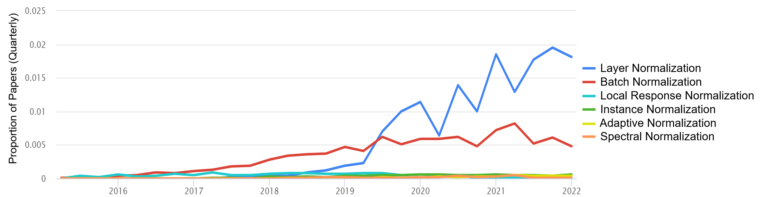
Figure 1. Trend in using normalization methods (Stojnic et al., 2022)

Batch normalization can be used to manipulate the statistical properties of layer activations. Well-designed statistical properties can represent the domain-specific information for the distribution of a group of inputs. More explicitly, batch normalization tries to force the activations of a layer into a gaussian unit distribution at the beginning of training. It standardizes the activations of DNN intermediate layers with an approach of a three-step computation:
1. Computation of Statistics: the mean and variance of each mini-batch during the training phase are calculated. Let $x$ denote inputs over a minibatch $B$ of size $m,B=\left\{x_{1},x_{2},\ldots,x_{m}\right\}$, each input with a dimension of $\left(x^{(1)},\ldots,x^{(d)}\right)$. Batch normalization (Ioffe and Szegedy, 2015) standardizes the mini-batch data by:

(1) $$\mu_{{B}}^{({k})}=\frac{1}{{~{}m}}\sum_{{i}=1}^{{m}}{x}_{{i}}^{({k})}\hskip 28.45274pt\sigma_{{B}}^{({k})^{2}}=\frac{1}{{~{}m}}\sum_{{i}=1}^{{m}}\left({x}_{{i}}^{({k})}-\mu_{{B}}^{({k})}\right)^{2}$$

Then, each dimension of the input is normalized separately:

(2) $$\hat{{x}}_{{i}}^{({k})}=\frac{{x}_{{i}}^{({k})}-\mu_{{B}}^{({k})}}{\sqrt{\sigma_{{B}}^{({k})^{2}}+\epsilon}}$$

where ${k}\in[1,{~{}d}]$ and ${i}\in[1,{~{}m}];$ $\mu_{{B}}^{({k})}$ and $\sigma_{{B}}^{({k})^{2}}$ are the per-dimension mean and variance, and $\epsilon>0$ is a small number to prevent numerical instability, respectively.
2. Batch Normalization Transform: batch normalization utilizes two additional learnable parameters to reconstitute a possible reduced representational capacity (Liao et al., 2016). Scale parameter $\gamma\in$ ${R}$ and shift parameter $\beta\in{R}$ where $\gamma$ and $\beta$ are subsequently learned in the optimization process.

(3) $${y}_{{i}}^{({k})}=\gamma^{({k})}\hat{{x}}_{{i}}^{({k})}+\beta^{({k})}$$

The output of the transform step is then passed to other network layers, while the normalized output remains internal to the current layer.
3. Inference: the normalization steps depend on mini-batches in the training phase. In the inference phase, however, this dependence is no longer helpful. Instead, the normalization step in this phase is calculated deterministically. The population mean $E\left[x^{(k)}\right]$ and variance $\operatorname{Var}\left[x^{(k)}\right]$ are estimated by calculating the moving averages of the summed input statistics:

(4) $${E}\left[{x}^{({k})}\right]={E}_{{B}}\left[\mu_{{B}}^{({k})}\right]$$

(5) $$\operatorname{Var}\left[x^{(k)}\right]=\frac{m}{m-1}E_{B}\left[\sigma_{B}^{(k)^{2}}\right]$$

Thus, the population statistics are a complete representation of all mini-batches. Therefore, the batch normalization transform in the inference step becomes:

(6) $${y}^{({k})}=\frac{\gamma^{({k})}}{\sqrt{\operatorname{Var}\left[{x}^{({k})}\right]+\epsilon}}{x}^{({k})}+\left(\beta^{({k})}-\frac{\gamma^{({k})}{E}\left[{x}^{({k})}\right]}{\sqrt{\operatorname{Var}\left[{x}^{({k})}\right]+\epsilon}}\right)\equiv{BN}_{\gamma^{(k)},\beta^{(k)}}^{{inference}}\left({x}^{({k})}\right)$$

where $y^{(k)}$ is passed to future layers instead of $x^{(k)}$. Since the parameters are fixed in this transformation, the batch normalization procedure applies a linear map to the activation.

Batch normalization has several advantages, including improving training stability, which is mainly due to its scale-invariant property (Gitman and Ginsburg, 2017; Yong et al., 2020; Neyshabur et al., 2016; Wan et al., 2021), meaning a bad input from the previous layer does not ruin the next layer. Although the practical success of batch normalization is undeniable and is present in current state-of-the-art architectures pervasively, its theoretical analysis remains limited. For example, in the case of optimization, most analyses require the model to be independent of input data, such that the stochastic/mini-batch gradient becomes an unbiased estimator of the true gradient over a dataset. However, batch normalization typically does not fit this data-independent assumption, and its optimization usually depends on the sampling strategy and the mini-batch size (Russakovsky et al., 2015). Furthermore, batch normalization still struggles with some problems in certain contexts. For example, the inconsistent operation of batch normalization between training and inference restricts its suitability in complex networks such as recurrent neural networks (Gitman and Ginsburg, 2017; Cooijmans et al., 2017; Laurent et al., 2016; Kurach et al., 2019; Salimans et al., 2016; Bhatt et al., 2019).

In order to address the drawbacks of batch normalization, layer normalization was introduced to estimate the normalization statistics directly from the summed inputs to the neurons within a hidden layer across all features. In layer normalization, all hidden units in a layer (mostly feature layer) have the same normalization statistics, which can be different in each training step (Gitman and Ginsburg, 2017). In other words, batch normalization converts to layer normalization with only two steps:
1. Computation of Statistics: the mean and variance used for normalization are computed from all summed inputs to the neurons on each training step. Let $x$ denote inputs over a minibatch $B$ of size $m,B=\left\{x_{1},x_{2},\ldots,x_{m}\right\}$, each input with a dimension of $\left(x^{(1)},\ldots,x^{(d)}\right)$, where ${i}\in[1,{~{}m}]$, and ${k}\in[1,{~{}d}]$. The mean and variance are computed as follows:

(7) $$\mu_{F}^{(i)}=\frac{1}{d}\sum_{k=1}^{d}x_{i}^{({k})}\\ \hskip 27.03003pt\sigma_{F}^{({i})^{2}}=\frac{1}{d}\sum_{k=1}^{d}\left(x_{i}^{({k})}-\mu_{F}^{(i)}\right)^{2}$$

Then, each sample is normalized such that the elements in the sample have zero mean and unit variance.

(8) $$\hat{x}_{{i}}^{({k})}=\frac{{x}_{{i}}^{({k})}-\mu_{F}^{(i)}}{\sqrt{\sigma_{F}^{({i})^{2}}+\epsilon}}$$

2. Transform: by applying transformation on the normalized inputs using some learned parameters $\gamma$ and $\beta$, the output could be expressed as ${B}^{\prime}=\left\{{y}_{1},{y}_{2},\ldots,{y}_{{m}}\right\}$, where ${y}_{{i}}=$ ${LN}_{\gamma,\beta}\left({x}_{{i}}\right)$.

(9) $$y_{i}=\gamma\hat{x}_{i}+\beta\equiv LN_{\gamma,\beta}\left(x_{i}\right)$$

Layer normalization performs the exact computation at training and inference times and does not require the moving averages of summed input statistics. In contrast to batch normalization, layer normalization is not subject to any restriction regarding the size of mini-batches and can be used in pure online mode with the batch size of one. Layer normalization has also proven to be an effective method for stabilizing the hidden state dynamics in recurrent neural networks. From an empirical point of view, it shows that it can significantly reduce the training time compared to previously published techniques (Gitman and Ginsburg, 2017). Despite the increasing usage of layer normalization in common neural network architectures (Vaswani et al., 2017; Al-Rfou et al., 2019; Yang et al., 2019) employed for NLP, layer normalization works not as well as batch normalization when used with convolutional layers. When layers are fully connected, all layers’ hidden units generally contribute similarly to the final prediction, and normalizing of summed inputs in a layer works well. However, similar contributions no longer hold for Convolutional Neural Networks (Gitman and Ginsburg, 2017).

The following section describes the theoretical assumptions and practical experiments of developing the new normalization method in overcoming the drawbacks of batch and layer normalization methods and having a new normalization technique that embodies the advantages of both methods in the area of Convolutional Neural Networks (CNNs) and Recurrent Neural Networks (RNNs).

3. Methodology

This study introduces a new normalization mechanism called BLN, in which batch and layer normalization methods are combined into one method that overcomes the disadvantages of each method and embraces the advantages of both of them. In batch settings, where a model is trained on the steps of an entire training set, we would use the whole training set to normalize the activations, which is impractical in stochastic optimization. Since we use mini-batches in stochastic gradient training and each mini-batch has estimates for the mean and variance of each activation. Therefore, the batch normalization authors simplified and used mini-batches statistics for normalization. One issue they did not consider was the size of mini-batches. As discussed, batch normalization has the problem of small batch size, and its error increases rapidly as the batch size gets smaller (Ulyanov et al., 2016). In contrast to batch normalization, layer normalization is not subject to any restriction regarding the size of mini-batches and can be used with the batch size of one.

To address this limitation in our new normalization method, we consider the size of mini-batches in calculating normalization through one essential step, in which activations are independently normalized on mini-batch (Equation. 14) and features (Equation. 15) by having the mean equal to zero and the variance equal to one. Next, these normalized activations are combined based on a function (the numerator of Equation. 16) of the inverse size of mini-batches, which acts as a parameter in the range of $\epsilon$ to $1-\epsilon$ to put the appropriate weights on the normalized activations of mini-batch $\left(\hat{x}\right)$ and features $\left(\hat{\vphantom{\rule{1.0pt}{5.5pt}}\smash{\hat{x}}}\right)$. The function’s behavior is shown in Figure 2 for the size of mini-batches ranging from 1 to 50. As shown in Figure 2, increasing the size of the mini-batches increases the weight put on mini-batch normalization, while its decrease causes an increase in the amount of weight on feature normalization.

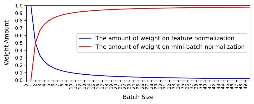
Figure 2. Effect of the numerator of Equation 16. on mini-batch and feature normalization.

To adaptively control the scaling weights for different layers, we divided the numerator of Equation. 16 by the root mean square of $d$ (the last dimensional shape of input), based on the idea presented in the AdaNorm algorithm (Xu et al., 2019). The issue of the normalizing equation (Equation. 16) is that a gradient descent optimization does not take into account the fact that normalizations occur. To solve this problem, the gradient of loss with respect to model parameters has to consider the normalizations and their dependence on model parameters. Therefore, we used a pair of learnable parameters $\gamma,\beta$ (Equation. 17) that scale and shift the normalized values for each input. Formally, let $x$ denote inputs over a minibatch $B$ of size $m,B=\left\{x_{1},x_{2},\ldots,x_{m}\right\}$, each input with a dimension of $\left(x^{(1)},\ldots,x^{(d)}\right)$, where ${i}\in[1,{~{}m}]$, ${k}\in[1,{~{}d}]$, and $\epsilon>0$ is a small number to avoid numerical instability, $\gamma$ and $\beta$ are parameters to be learned. We compute output $\left\{y_{i}=BLN_{\gamma,\beta}\left(x_{i}\right)\right\}$ with Algorithm 1.

Input: Inputs over a mini-batch: $B=\left\{x_{1},x_{2},\ldots,x_{m}\right\}$, each with a dimension of $\left(x^{(1)},\ldots,x^{(d)}\right)$; Parameters to be learned: ${\gamma,\beta}$
Output: $\left\{y_{i}=BLN_{\gamma,\beta}\left(x_{i}\right)\right\}$
$\mu_{{B}}^{({k})}\leftarrow\frac{1}{{~{}m}}\sum_{{i}=1}^{{m}}{x}_{{i}}^{({k})}$                                                                                   mini batch mean (10)
$\sigma_{{B}}^{({k})}\leftarrow\sqrt{\frac{1}{{~{}m}}\sum_{{i}=1}^{{m}}\left({x}_{{i}}^{({k})}-\mu_{{B}}^{({k})}\right)^{2}+\epsilon}$                                                  mini-batch standard deviation (11)
$\mu_{F}^{(i)}\leftarrow\frac{1}{d}\sum_{k=1}^{d}x_{i}^{({k})}$                                                                                        feature mean (12)
$\sigma_{F}^{({i})}\leftarrow\sqrt{\frac{1}{d}\sum_{k=1}^{d}\left(x_{i}^{({k})}-\mu_{F}^{(i)}\right)^{2}}$                                                             feature standard deviation (13)
$\hat{x}^{{(k)}}_{{i}}\leftarrow\frac{{x}_{{i}}^{({k})}-\mu_{{B}}^{({k})}}{\sigma_{{B}}^{({k})}}$                                                                                  normalize mini-batch (14)
$\hat{\vphantom{\rule{1.0pt}{5.5pt}}\smash{\hat{x}}}^{{(k)}}_{{i}}\leftarrow\frac{{x}_{{i}}^{({k})}-\mu_{F}^{(i)}}{\sigma_{F}^{({i})}}$                                                                                     normalize features (15)
$\hat{\vphantom{\rule{1.0pt}{5.5pt}}\smash{\hat{\hat{x}}}}_{i}\leftarrow\frac{\left(\left(1-\left(\frac{1}{m}+\epsilon\right)\right)\hskip 1.42271pt\hat{x}_{{i}}\right)+\left(\left(\frac{1}{m}-\epsilon\right)\hskip 1.42271pt\hat{\hat{x}}_{{i}}\right)}{\sqrt{d}}$                                                                              normalize (16)
${y}_{{i}}\leftarrow\gamma\hskip 5.69046ptx\hat{\vphantom{\rule{1.0pt}{5.5pt}}\smash{\hat{\hat{}}}}_{i}+\beta\equiv{BLN}\gamma,\beta\left({x}_{{i}}\right)$                                                                              scale and shift (17)

Algorithm 1 Batch Layer Normalization Transform.

The authors of the batch normalization method generally assume that the normalization of activations depends on mini-batch statistics during training but is never essential during inference (Ioffe and Szegedy, 2015). They used during inference, population statistics rather than mini-batch statistics. Various studies (Gitman and Ginsburg, 2017; Cooijmans et al., 2017; Laurent et al., 2016; Kurach et al., 2019; Salimans et al., 2016; Bhatt et al., 2019) have been conducted, showing that using population statistics works well with CNNs, but they do not work well for NLP tasks that use RNNs (Cooijmans et al., 2017; Shen et al., 2020) on account of the recurrent connection to previous time stamps. For example, in a study (Cooijmans et al., 2017) used moving batch statistics for different time steps of RNNs, it was found that the performance of a batch normalization method is significantly lower than that of a layer normalization method. We also had the experience that a change such as using batch statistics instead of a global average of summed input statistics in the inference phase of a batch normalization method affects the performance of a model.

On the other hand, the authors of the layer normalization method assume that the normalization of activations depends only on mini-batch statistics during training and inference (Ba et al., 2016). Thus, it can be inferred that the assumption that normalizing activations during inference must always depend on the population of the entire training set is not entirely correct. To address this issue, we also note that previous works have thoroughly investigated the role of normalization methods in models’ hyper-parameter optimization processes as a relatively unexplored parameter. Therefore, we give Batch Layer Normalization a role in the hyper-parameter optimization process of a model by selecting between two assumptions for each of all four statistics (4² possible configurations) in Algorithm 1. In the first assumption, for the normalization of activations during inference, mean or standard deviation is obtained from the corresponding estimated population statistics by setting True in one of the Equations $18,19,20,21$ (see Appendix), where the expectations are over training mini-batches of size $m$ and $\mu_{B},\sigma_{B},\mu_{F},\sigma_{F}$ are their sample means and standard deviations on mini-batches and features (Equations 10, 11, 12, 13). In the second, mean or standard deviation is only taken from the statistics of mini-batch during inference by selecting False in one of the Equations $18,19,20,21$ (see Appendix). The selection process can be assumed as a hyper-parameter optimization process to fine-tune a model, leading to stabilization and further improvement of the model. Next, the normalization (Equations 22, 23, 24 in Appendix) is applied to each input, which is further composed with the scaling by $\gamma$ and shift by $\beta$ to form a single linear transform that replaces BLN($x_{i}$). The described procedure for training a Batch Layer Normalization network is summarized in Algorithm 2.

As shown in Equation. 26, batch normalization (Ioffe and Szegedy, 2015) suggests that the normalization layer can be placed before activation functions such as sigmoid or ReLU for both fully-connected and convolutional layers. Therefore, they add the batch normalization transform before the nonlinearity ${g}(.)$, where ${W}$ and ${b}$ are learned parameters of a model and ${u}$ is the layer inputs.

(26) $${z}={g}({BN}({Wu}+{b}))$$

In a study that shows the impact of recent advances in CNN architectures and learning methods (Mishkin et al., 2017), the authors conduct comparative experiments on the ImageNet dataset (Russakovsky et al., 2015) to understand whether a batch normalization method should be placed before or after the nonlinearity. The experiment showed that batch normalization placement after the nonlinearity results in better accuracy. Therefore, we apply the BLN transform after the nonlinearity $g(.)$ in contrast to batch normalization.

(27) $${z}={BLN}({g}({Wu}+{b}))$$

4. Experiments

This section aims to first evaluate BLN to the internal covariate shift problem of deep learning layers, second to compare it to the application of batch and layer normalization method, and finally, draw conclusions from the results about the applicability of the new method for better solving the problem of internal covariate shift. As mentioned earlier, batch normalization works well with CNNs and has the problem of not working with small batch sizes and RNNs; in contrast, layer normalization works well with RNNs and small batch sizes and has the disadvantage of not working well with CNNs. To test the applicability of our method, both with Convolutional and Recurrent Neural Networks and different batch sizes, two different challenging experiments were designed. The first is in the image classification area using the CIFAR-10 (Krizhevsky et al., 2009) dataset, and the second is in the domain of sentiment analysis on the IMDB movie review dataset. Furthermore, to ensure the validity of the results in each experiment, we use identical architectures, training hyper-parameters, optimizations, and grid-search algorithms but different normalization methods. For all experiments, we set $\epsilon$ in all Equation to be 0.0001 and train all networks from scratch using an Adam optimizer with batch sizes of 1 and 25.

4.1. Classifying CIFAR-10 using CNN

To compare BLN against the other two approaches, batch and layer normalization in image classification and CNNs, we borrowed the popular LeNet-5 (El-Sawy et al., 2017) architecture. Since there is no normalization layer in the original LeNet architecture, we derived a modified model from it (Figure 3) so that a normalization layer is embedded after some layers. By replacing the embedded normalization layers in the modified network with one of the discussed normalization methods, batch, layer, and BLN method, three independent networks were obtained in terms of normalization methods for each normalizer. Note that hyper-parameters and architectures used in training these networks are the same to ensure that the effect of these normalizers is compared appropriately.

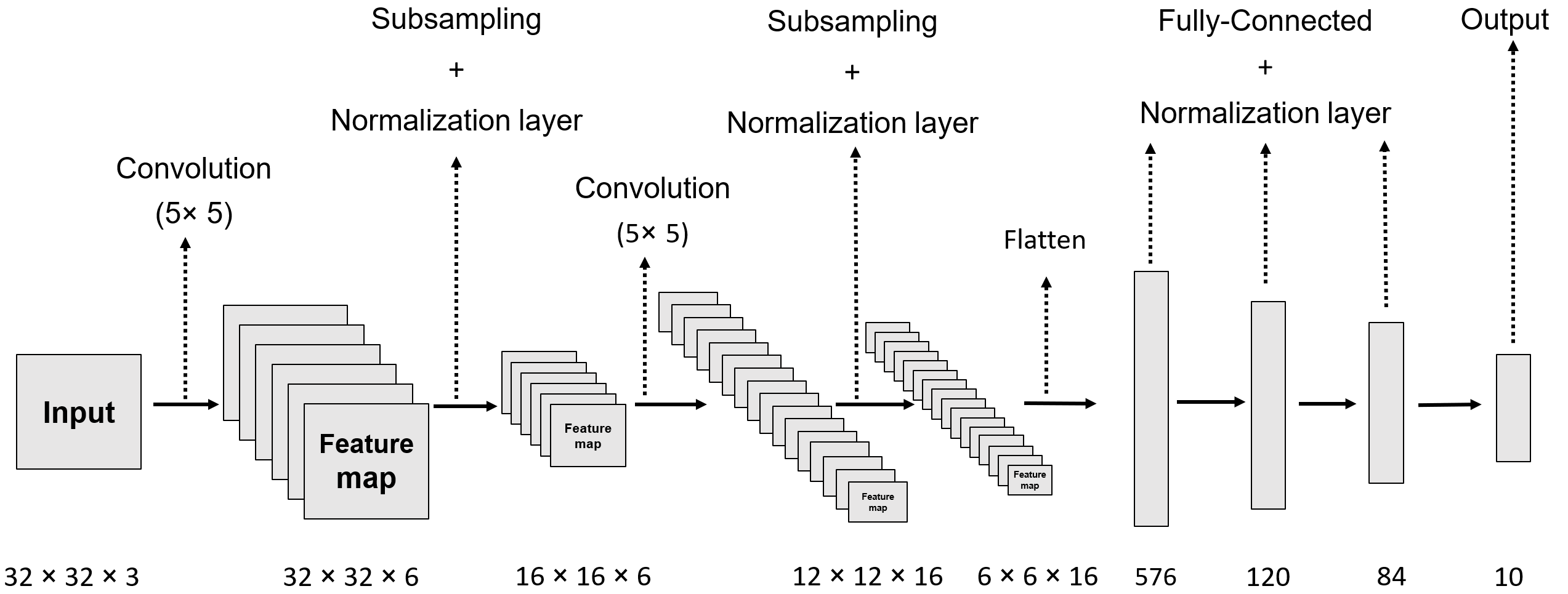
Figure 3. Illustration of modified LeNet architecture.

As proof of the challenging experiments, after training each network independently on only 20% of the training dataset with batch sizes of 1 and 25, we compared their training results, including convergence issues and classification accuracy, as well as their performances on the whole CIFAR-1O test set. Loss results presented in Figure 4 show that BLN significantly accelerates the neural network training and accomplishes a step toward reducing the internal covariant shift problem. In other words, considering the size of mini-batches in the calculation of normalization reduces the probability of getting stuck in the saturation regime and thus stimulates the training process. Figure 4 also indicates that batch normalization with a batch size of 25 performs better than layer normalization. This finding notably confirms that in the case of big batch sizes, batch normalization has been the de facto standard for CNNs. Conversely, using batch normalization in CNNs significantly degrades the model’s performance when batch size is one.

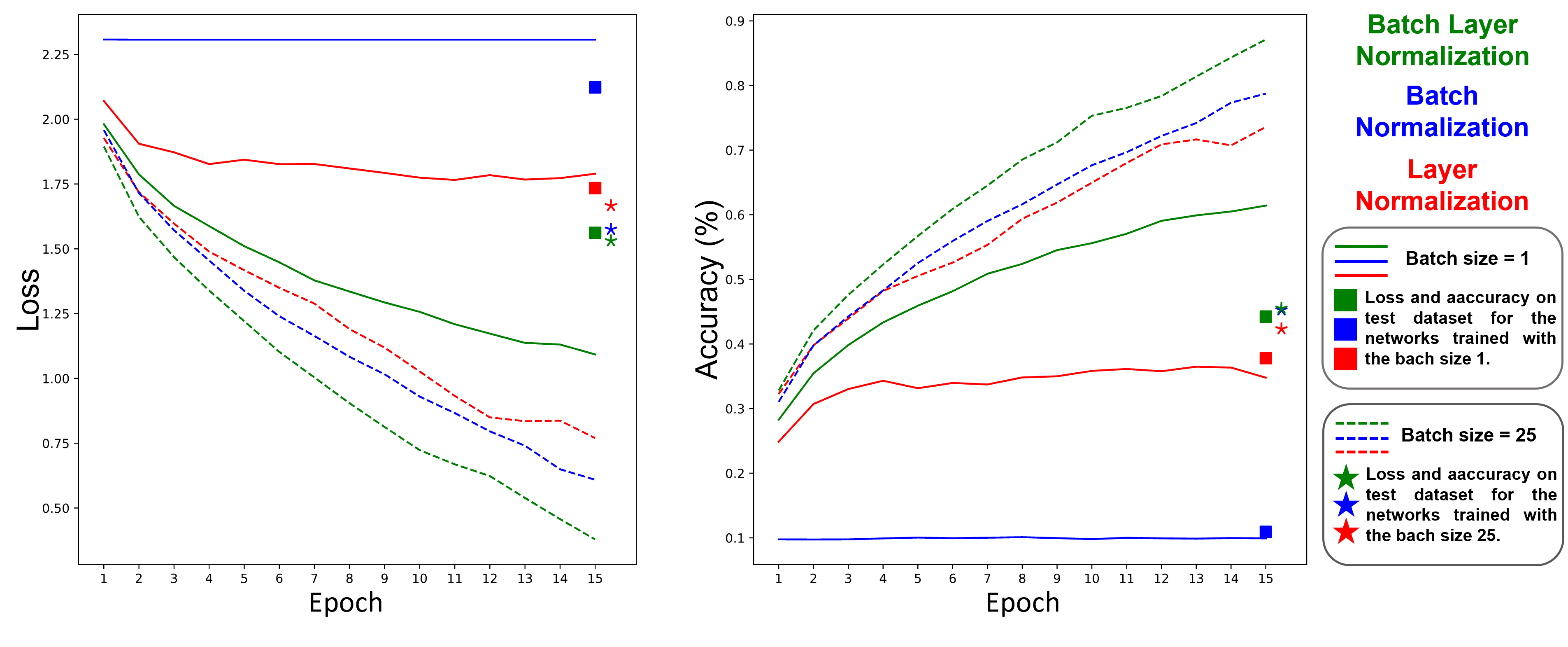
((a)) Train and Test loss

((b)) Train and Test accuracy

Figure 4. Loss and Accuracy on training and test dataset.

Based on Figure 4, which shows the experimental results in terms of the training and test accuracy, BLN enables the model to train faster and achieve higher accuracies of 0.61 and 0.87, while batch normalization achieves 0.09 and 0.78 and layer normalization scores 0.34 and 0.73 on the training set with batch sizes 1 and 25, respectively. Moreover, BLN obtains better test accuracy compared to other normalizers.

Table 1 shows the possible configurations (step 12 of Algorithm 2) for the BLN network trained on either the entire training dataset or 20% of it with a batch size of 25. These configurations are found using the grid-search approach and sorted in terms of lower loss and higher accuracy on the entire test dataset. According to Table 1, the training data size significantly impacts finding the best configuration of the BLN statistics in support of the theoretical analysis of independent input data and improving the practical results.

Table 1. Configurations of BLN statistics used in CNN task.

	20% of the training set used to train with a batch size of 25					Whole training set used to train with a batch size of 25
A	${E}_{B}$	$\operatorname{Std}_{B}$	${E}_{{F}}$	$\operatorname{Std}_{{F}}$	B	${E}_{B}$	$\operatorname{Std}_{B}$	${E}_{{F}}$	$\operatorname{Std}_{{F}}$
1	True	True	False	False		False	True	False	False
2	True	True	False	True		False	True	False	True
3	True	True	True	True		False	True	True	True
4	True	True	True	False		False	True	True	False
5	False	False	False	True		False	False	False	False
6	False	False	False	False		False	False	False	True
7	False	False	True	True		False	False	True	True
8	False	False	True	False		False	False	True	False
9	False	True	False	True		True	True	False	True
10	False	True	False	False		True	True	False	False
11	False	True	True	True		True	True	True	True
12	False	True	True	False		True	True	True	False
13	True	False	True	False		True	False	True	False
14	True	False	True	True		True	False	True	True
15	True	False	False	True		True	False	False	True
16	True	False	False	False		True	False	False	False

As shown in part B of Table 1, the first-best possible configuration reveals that when using the whole training data, the current batch mean (${E}_{B}$ = False) and feature mean (${E}_{{F}}$ = False) are suitable settings to be used in the inference to normalize the input to layers of the network. The intuition is that the obtained global mean on batches and features may not share general information. In contrast, when using 20% of the whole training set (part A of Table 1), the first-best configuration suggests utilizing the population statistics on batches (${E}_{B}$ = True, $\operatorname{Std}_{B}$ = True) since we are using a subset of the training dataset and this information can assist the model in converging faster and learning better. Accordingly, this conclusion can be broadly applied to other statistic configurations of Table 1. For example, the first-best and second-best configuration of the statistics show no advantage of using the population mean of features in both cases when the whole data or 20% of it is used.

4.2. Sentiment analysis of IMDB using RNN

To investigate the performance and correlation between the statistical properties of BLN in the NLP domain, a sentiment analysis task was developed using an RNN with a focus on challenging the intriguing phenomenon that layer normalization is more effective than batch normalization in the NLP domain (Gitman and Ginsburg, 2017), against the BLN method. Three independent networks were obtained by replacing all the normalization layers in the RNN architecture (Figure 5) with one of the normalization methods discussed. These networks were trained and evaluated on the IMDB movie review dataset that contains 50,000 reviews divided equally across train and test splits. As a note, the experimental protocol described in Section 4.1 was used for all experiments.

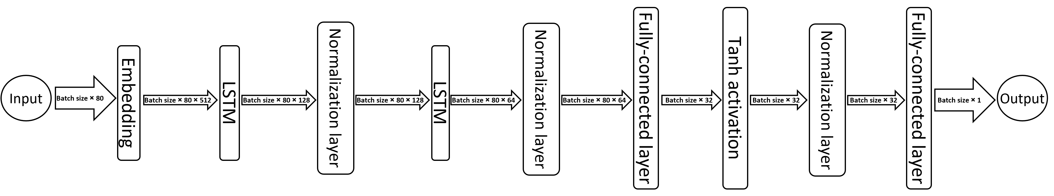
Figure 5. Illustration of proposed RNN architecture.

Figure 6 and 6 show the loss and accuracy of the obtained networks trained on 20% of the training dataset and evaluated on the whole test dataset with batch sizes of 1 and 25. As shown, BLN offers a per-iteration speedup and converges faster than batch normalization and even layer normalization, which is the most commonly used normalizer in the NLP domain. Based on the final results, our BLN normalizer shows significant improvement compared to the other two normalizers in all train and test evaluation metrics.

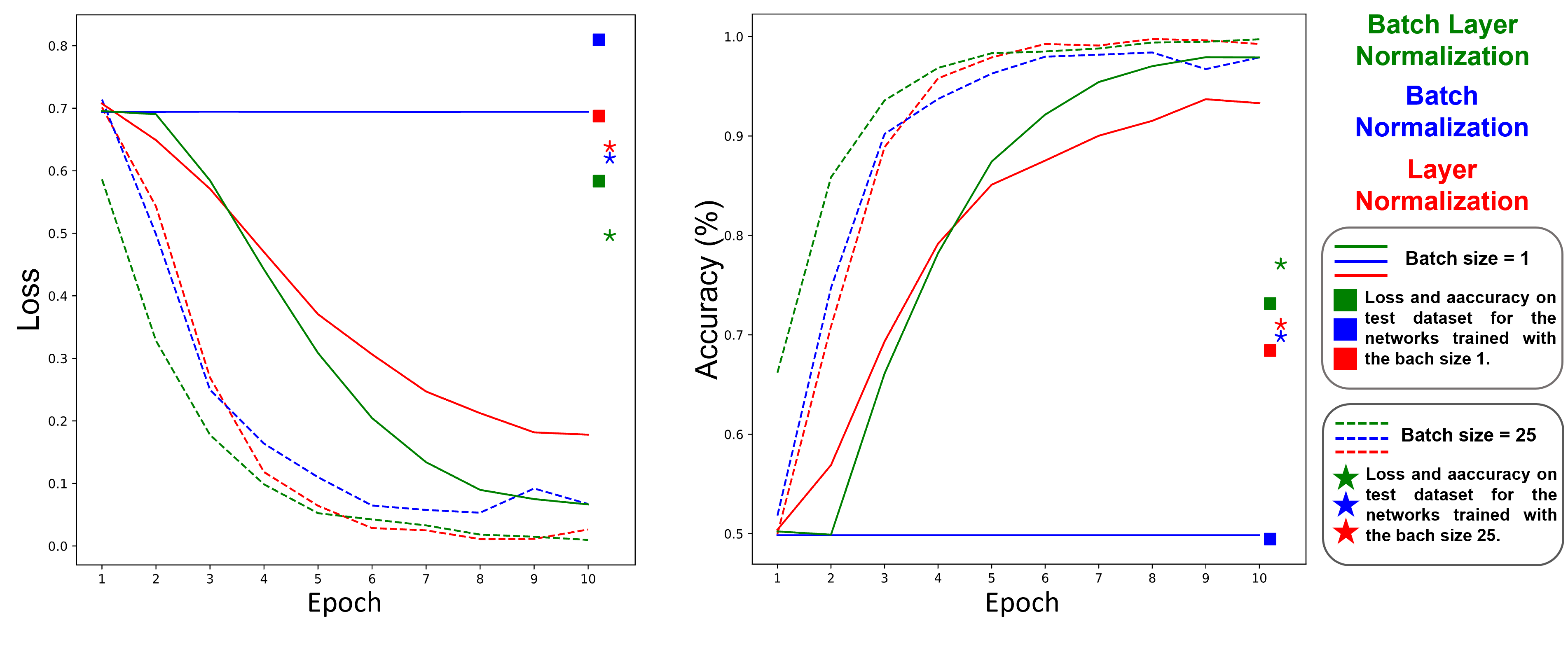
((a)) Train and Test loss

((b)) Train and Test accuracy

Figure 6. Loss and Accuracy on training and test dataset.

As demonstrated in Figures 6 and 6, the layer normalization potentially performs better than the batch normalization in terms of loss and accuracy. This result confirms the discussed assumption that layer normalization in RNNs improves the model’s performance. Table 2. summarizes the possible configurations (step 12 of Algorithm 2) for the BLN network trained on either the entire training dataset or 20% of it with a batch size of 25. These configurations are found using the grid-search approach and sorted in terms of lower loss and higher accuracy on the entire test dataset. Inferring from this table, we observe that the current batch mean (${E}_{{B}}$ = False) is a suitable configuration in the normalization process of the sentiment analysis task and elevates the performance while the global batch mean does not pass general information to the model or is not helpful at all for RNNs. In contrast, we recommend not using the global mean statistic obtained from the moving mean of batches when using either the whole training set or a subset of it. This deduction can broadly be extended to other sets of statistics.

Table 2. Configurations of BLN statistics used in RNN task.

	20% of the training set used to train with a batch size of 25					Whole training set used to train with a batch size of 25
A	${E}_{B}$	$\operatorname{Std}_{B}$	${E}_{{F}}$	$\operatorname{Std}_{{F}}$	B	${E}_{B}$	$\operatorname{Std}_{B}$	${E}_{{F}}$	$\operatorname{Std}_{{F}}$
1	False	False	True	False		False	True	False	False
2	False	False	False	False		False	True	True	False
3	False	False	True	True		False	True	False	True
4	False	False	False	True		False	True	True	True
5	True	False	False	True		False	False	False	True
6	True	False	True	True		False	False	True	True
7	True	False	False	False		False	False	False	False
8	True	False	True	False		False	False	True	False
9	False	True	True	False		True	True	False	False
10	False	True	False	False		True	True	True	False
11	False	True	True	True		True	True	False	True
12	False	True	False	True		True	True	True	True
13	True	True	False	False		True	False	False	True
14	True	True	True	False		True	False	True	True
15	True	True	False	True		True	False	False	False
16	True	True	True	True		True	False	True	False

5. Discussion

The experimental results show that BLN converges significantly faster than batch and layer normalization in both CNN and RNN domains. Figures 4 and 6 also indicate that considering the size of mini-batches when calculating the normalization can contribute to finding the best statistical configuration, which leads to fast convergence of BLN. Furthermore, Tables 1 and 2 also show that the assumption that normalization of activations during inference must always depend on mini-batch statistics or population statistics is not a solid general assumption and must be modified according to the task, the amount of training data and the size of batches. These results notably approve that BLN supports the theoretical analysis of being independent of the input data by configuring its statistics used in the normalization process strongly based on the task, training data, and batch sizes. Complementary to this main point, other outcomes can be summarized as follows:

1. From the first-best configuration in parts A and B of Table 1, taking the global mean and standard deviation of features (${E}_{{F}}$ = True, $\operatorname{Std}_{{F}}$ = True) in CNN normalization is not recommended regardless of training data size. In summary, the global batch mean is generally a good statistic for normalizing CNNs, when the training data is small, and vice versa; the current batch mean when the training data is big enough.

2. The first-best configurations in parts A and B of Table 2 declare that while utilizing the population mean on batches (${E}_{{B}}$ = True) in RNN normalization is not a good idea at all, the current mean and standard deviation of features can help RNNs converge faster.

3. The first-best configurations in both parts (A and B) of Tables 1 and 2 approve that using the current standard deviation of features ($\operatorname{Std}_{{F}}$ = False) in normalization can usually help CNNs and RNNs converge faster.

The limitation of BLN can be reflected in the time spent searching for the best configuration of statistics. This time can be reduced using the heuristic hyper-parameter tuning methods (Yu and Zhu, 2020). In future work, step 12 of Algorithm 2, which is tailored to overall neural network architecture, can also be extended to the statistics used for each deep neural network layer.

6. Conclusions

In this paper, we proposed a novel normalization method called BLN to reduce the internal covariate shift in deep learning layers and significantly accelerate their training. As a normalization layer, BLN not only exploits the advantages of the two most commonly used normalizers in the deep learning networks, batch, and layer normalization but also suppresses their drawbacks. Our proposed method derives its strength during training from appropriate weighting on mini-batch and feature normalization based on the inverse size of mini-batches and integrating this normalization in the network architecture. This guarantees that the normalization is appropriately handled by each optimization method used to train the network. During inferences times, it also performs the exact computation with a slight modification, using either mini-batch or population statistics as a decision process to play a comprehensive role in hyper-parameter optimization of models. BLN’s main advantage is that it supports the theoretical analysis of being independent of the input data, as its statistical configuration is highly dependent on the task we are performing, the amount of training data, and the size of batches. We empirically verify that BLN is superior to using batch and layer normalization both in Convolutional and Recurrent Neural Networks, respectively, which further establishes the generalizability of our method in different deep learning models.

Appendix

Input: Network $N$ with trainable parameters $\theta$; subset of activations $\left\{x^{(\mathbf{k})}_{i}\right\}_{i=1,k=1}^{m,d}$
Output: Batch Layer Normalization network for inference, $N_{BLN}^{\inf}$
$1:{N}_{{BLN}}^{{tr}}\leftarrow{N}$                                                                     // Training BLN network
$2:$ for $i=1\ldots m$ do
00000$3:$ Add transformation $y_{i}=\operatorname{BLN}_{\gamma,\beta}\left(x_{i}\right)$ to $N_{BLN}{t{r}}($ Algorithm. 1)
00000$4:$ Modify each layer in $N_{BLN}^{\operatorname{tr}}$ with input $x_{i}$ to take $y_{i}$ instead
$5:$ end for
$6:$ Train $N_{BLN}^{tr}$ to optimize the parameters $\Theta\cup\left\{\gamma,\beta\right\}$
$7:$ $N_{BLN}^{\inf}\leftarrow N_{BLN}^{tr}$                                     // Inference BLN network with frozen parameters
$8:$ for $k=1\ldots d$ do

$9:$ Set ${E}_{B}[{x}^{({k})}]=$ False, $\operatorname{Std}_{B}[{x}^{({k})}]=$ False, ${E}_{{F}}[{x}_{{i}}]=$ False, $\operatorname{Std}_{{F}}[{x}_{{i}}]=$ False as initial parameters. For clarity, True means using population statistics (process multiple training mini-batches ${B}$, each of size ${m}$ and average over them), False means using of current mini-batch statistics.

$${E}_{B}[{x}^{({k})}]=\begin{cases}{E}\left[\mu_{B}^{({k})}\right]&\text{ if True }\\ \frac{1}{{~{}m}}\sum_{{i}=1}^{{m}}{x}_{{i}}^{({k})}&\text{False}\end{cases}\hskip 108.12054pt(18)$$

$$\operatorname{Std}_{B}[{x}^{({k})}]=\begin{cases}\frac{{m}}{{m}-1}{E}\left[\sigma_{{B}}^{({k})}\right]&\text{if True}\\ \sqrt{\frac{1}{{~{}m}}\sum_{{i}=1}^{{m}}\left({x}_{{i}}^{({k})}-{E}_{{B}}[{x}^{({k})}]\right)^{2}+\epsilon}&\text{False}\end{cases}\hskip 28.45274pt(19)$$

$${E}_{{F}}[{x}_{{i}}]=\begin{cases}{E}\left[\mu_{{F}}^{({i})}\right]&\text{if True}\\ \frac{1}{{~{}k}}\sum{x}_{{i}}^{({k})}&\text{False}\end{cases}\hskip 133.72786pt(20)$$

$$\operatorname{Std}_{{F}}[{x}_{{i}}]=\begin{cases}\frac{{m}}{{m}-1}{E}\left[\sigma_{{F}}^{({i})}\right]&\text{if True}\\ \sqrt{\frac{1}{k}\sum\left(x_{i}^{({k})}-{E}_{{F}}[{x}_{{i}}]\right)^{2}}&\text{False}\end{cases}\hskip 73.97733pt(21)$$

$$\hat{x}^{{(k)}}_{{i}}\leftarrow\frac{{x}_{{i}}^{{k}}-{E}_{B}[{x}^{({k})}]}{\operatorname{Std}_{{B}}[{x}^{({k})}]}\hskip 162.18062pt(22)$$

$$\hat{\hat{x}}^{{(k)}}_{{i}}\leftarrow\frac{{x}_{{i}}^{{k}}-{E}_{F}[{x}_{{i}}]}{\operatorname{Std}_{{F}}[{x}_{{i}}]}\hskip 170.71652pt(23)$$

$10:$ end for
$11:$ In ${N}_{{BL}N}^{{inf}}$, replace the transform $y_{i}=\operatorname{BLN}_{\gamma,\beta}({x_{i}})$ with

$$x\hat{\vphantom{\rule{1.0pt}{5.5pt}}\smash{\hat{\hat{}}}}_{i}\leftarrow\frac{\left(\left(1-\left(\frac{1}{m}+\epsilon\right)\right)\hskip 1.42271pt\hat{x}_{{i}}\right)+\left(\left(\frac{1}{m}-\epsilon\right)\hskip 1.42271pt\hat{\hat{x}}_{{i}}\right)}{\sqrt{d}}\hskip 98.16191pt(24)\\$$

$${y}_{{i}}\leftarrow\gamma\hskip 5.69046ptx\hat{\vphantom{\rule{1.0pt}{5.5pt}}\smash{\hat{\hat{}}}}_{i}+\beta\hskip 197.74655pt(25)$$

$12:$ Use a grid-search algorithm or other hyper-parameter tuning techniques (Yu and Zhu, 2020) to find the best configuration of statistics (${E}_{B}$, $\operatorname{Std}_{B}$, ${E}_{{F}}$, $\operatorname{Std}_{{F}}$) among the possible configurations with lower loss and higher accuracy.
13: Use the best configuration for the rest of the training or fine-tuning and network testing.

Algorithm 2 Batch Layer Normalization Transform.

References

- (1)
- Al-Rfou et al. (2019) Rami Al-Rfou, Dokook Choe, Noah Constant, Mandy Guo, and Llion Jones. 2019. Character-Level Language Modeling with Deeper Self-Attention. In Proceedings of the Thirty-Third AAAI Conference on Artificial Intelligence and Thirty-First Innovative Applications of Artificial Intelligence Conference and Ninth AAAI Symposium on Educational Advances in Artificial Intelligence (Honolulu, Hawaii, USA) (AAAI’19/IAAI’19/EAAI’19). AAAI Press, Article 388, 8 pages. https://doi.org/10.1609/aaai.v33i01.33013159
- Arpit et al. (2016) Devansh Arpit, Yingbo Zhou, Bhargava Kota, and Venu Govindaraju. 2016. Normalization Propagation: A Parametric Technique for Removing Internal Covariate Shift in Deep Networks. In Proceedings of The 33rd International Conference on Machine Learning (Proceedings of Machine Learning Research, Vol. 48), Maria Florina Balcan and Kilian Q. Weinberger (Eds.). PMLR, New York, New York, USA, 1168–1176. https://proceedings.mlr.press/v48/arpitb16.html
- Ba et al. (2016) Lei Jimmy Ba, Jamie Ryan Kiros, and Geoffrey E. Hinton. 2016. Layer Normalization. CoRR abs/1607.06450 (2016). arXiv:1607.06450 http://arxiv.org/abs/1607.06450
- Bhatt et al. (2019) Aditya Bhatt, Max Argus, Artemij Amiranashvili, and Thomas Brox. 2019. CrossNorm: Normalization for Off-Policy TD Reinforcement Learning. CoRR abs/1902.05605 (2019). arXiv:1902.05605 http://arxiv.org/abs/1902.05605
- Chang et al. (2015) Angel X. Chang, Thomas A. Funkhouser, Leonidas J. Guibas, Pat Hanrahan, Qi-Xing Huang, Zimo Li, Silvio Savarese, Manolis Savva, Shuran Song, Hao Su, Jianxiong Xiao, Li Yi, and Fisher Yu. 2015. ShapeNet: An Information-Rich 3D Model Repository. CoRR abs/1512.03012 (2015). arXiv:1512.03012 http://arxiv.org/abs/1512.03012
- Cooijmans et al. (2017) Tim Cooijmans, Nicolas Ballas, César Laurent, Çaglar Gülçehre, and Aaron C. Courville. 2017. Recurrent Batch Normalization. In 5th International Conference on Learning Representations, ICLR 2017, Toulon, France, April 24-26, 2017, Conference Track Proceedings. OpenReview.net. https://openreview.net/forum?id=r1VdcHcxx
- El-Sawy et al. (2017) Ahmed El-Sawy, Hazem EL-Bakry, and Mohamed Loey. 2017. CNN for Handwritten Arabic Digits Recognition Based on LeNet-5. In Proceedings of the International Conference on Advanced Intelligent Systems and Informatics 2016, Aboul Ella Hassanien, Khaled Shaalan, Tarek Gaber, Ahmad Taher Azar, and M. F. Tolba (Eds.). Springer International Publishing, Cham, 566–575. https://doi.org/10.1007/978-3-319-48308-5_54
- Gitman and Ginsburg (2017) Igor Gitman and Boris Ginsburg. 2017. Comparison of Batch Normalization and Weight Normalization Algorithms for the Large-scale Image Classification. CoRR abs/1709.08145 (2017). arXiv:1709.08145 http://arxiv.org/abs/1709.08145
- He et al. (2016) Kaiming He, Xiangyu Zhang, Shaoqing Ren, and Jian Sun. 2016. Identity Mappings in Deep Residual Networks. In Computer Vision - ECCV 2016 - 14th European Conference, Amsterdam, The Netherlands, October 11-14, 2016, Proceedings, Part IV (Lecture Notes in Computer Science, Vol. 9908), Bastian Leibe, Jiri Matas, Nicu Sebe, and Max Welling (Eds.). Springer, 630–645. https://doi.org/10.1007/978-3-319-46493-0_38
- Hoffer et al. (2017) Elad Hoffer, Itay Hubara, and Daniel Soudry. 2017. Train longer, generalize better: closing the generalization gap in large batch training of neural networks. In Advances in Neural Information Processing Systems 30: Annual Conference on Neural Information Processing Systems 2017, December 4-9, 2017, Long Beach, CA, USA, Isabelle Guyon, Ulrike von Luxburg, Samy Bengio, Hanna M. Wallach, Rob Fergus, S. V. N. Vishwanathan, and Roman Garnett (Eds.). 1731–1741. https://proceedings.neurips.cc/paper/2017/hash/a5e0ff62be0b08456fc7f1e88812af3d-Abstract.html
- Huang et al. (2017) Gao Huang, Zhuang Liu, Laurens van der Maaten, and Kilian Q. Weinberger. 2017. Densely Connected Convolutional Networks. In 2017 IEEE Conference on Computer Vision and Pattern Recognition, CVPR 2017, Honolulu, HI, USA, July 21-26, 2017. IEEE Computer Society, 2261–2269. https://doi.org/10.1109/CVPR.2017.243
- Ioffe (2017) Sergey Ioffe. 2017. Batch Renormalization: Towards Reducing Minibatch Dependence in Batch-Normalized Models. In Advances in Neural Information Processing Systems, I. Guyon, U. Von Luxburg, S. Bengio, H. Wallach, R. Fergus, S. Vishwanathan, and R. Garnett (Eds.), Vol. 30. Curran Associates, Inc. https://proceedings.neurips.cc/paper/2017/file/c54e7837e0cd0ced286cb5995327d1ab-Paper.pdf
- Ioffe and Szegedy (2015) Sergey Ioffe and Christian Szegedy. 2015. Batch Normalization: Accelerating Deep Network Training by Reducing Internal Covariate Shift. In Proceedings of the 32nd International Conference on Machine Learning (Proceedings of Machine Learning Research, Vol. 37), Francis Bach and David Blei (Eds.). PMLR, Lille, France, 448–456. https://proceedings.mlr.press/v37/ioffe15.html
- Krizhevsky et al. (2009) Alex Krizhevsky, Vinod Nair, and Geoffrey Hinton. 2009. CIFAR-10 (Canadian Institute for Advanced Research). (2009). http://www.cs.toronto.edu/~kriz/cifar.html
- Kurach et al. (2019) Karol Kurach, Mario Lučić, Xiaohua Zhai, Marcin Michalski, and Sylvain Gelly. 2019. A Large-Scale Study on Regularization and Normalization in GANs. In Proceedings of the 36th International Conference on Machine Learning (Proceedings of Machine Learning Research, Vol. 97), Kamalika Chaudhuri and Ruslan Salakhutdinov (Eds.). PMLR, 3581–3590. https://proceedings.mlr.press/v97/kurach19a.html
- Laurent et al. (2016) César Laurent, Gabriel Pereyra, Philémon Brakel, Ying Zhang, and Yoshua Bengio. 2016. Batch normalized recurrent neural networks. In 2016 IEEE International Conference on Acoustics, Speech and Signal Processing (ICASSP). 2657–2661. https://doi.org/10.1109/ICASSP.2016.7472159
- Liao et al. (2016) Qianli Liao, Kenji Kawaguchi, and Tomaso A. Poggio. 2016. Streaming Normalization: Towards Simpler and More Biologically-plausible Normalizations for Online and Recurrent Learning. CoRR abs/1610.06160 (2016). arXiv:1610.06160 http://arxiv.org/abs/1610.06160
- Lin et al. (2014) Tsung-Yi Lin, Michael Maire, Serge J. Belongie, James Hays, Pietro Perona, Deva Ramanan, Piotr Dollár, and C. Lawrence Zitnick. 2014. Microsoft COCO: Common Objects in Context. In Computer Vision - ECCV 2014 - 13th European Conference, Zurich, Switzerland, September 6-12, 2014, Proceedings, Part V (Lecture Notes in Computer Science, Vol. 8693), David J. Fleet, Tomás Pajdla, Bernt Schiele, and Tinne Tuytelaars (Eds.). Springer, 740–755. https://doi.org/10.1007/978-3-319-10602-1_48
- Mishkin et al. (2017) Dmytro Mishkin, Nikolay Sergievskiy, and Jiri Matas. 2017. Systematic evaluation of convolution neural network advances on the Imagenet. Comput. Vis. Image Underst. 161 (2017), 11–19. https://doi.org/10.1016/j.cviu.2017.05.007
- Neyshabur et al. (2016) Behnam Neyshabur, Ryota Tomioka, Ruslan Salakhutdinov, and Nathan Srebro. 2016. Data-Dependent Path Normalization in Neural Networks. In 4th International Conference on Learning Representations, ICLR 2016, San Juan, Puerto Rico, May 2-4, 2016, Conference Track Proceedings, Yoshua Bengio and Yann LeCun (Eds.). http://arxiv.org/abs/1511.06747
- Qi et al. (2017) Charles Ruizhongtai Qi, Hao Su, Kaichun Mo, and Leonidas J. Guibas. 2017. PointNet: Deep Learning on Point Sets for 3D Classification and Segmentation. In 2017 IEEE Conference on Computer Vision and Pattern Recognition, CVPR 2017, Honolulu, HI, USA, July 21-26, 2017. IEEE Computer Society, 77–85. https://doi.org/10.1109/CVPR.2017.16
- Russakovsky et al. (2015) Olga Russakovsky, Jia Deng, Hao Su, Jonathan Krause, Sanjeev Satheesh, Sean Ma, Zhiheng Huang, Andrej Karpathy, Aditya Khosla, Michael S. Bernstein, Alexander C. Berg, and Li Fei-Fei. 2015. ImageNet Large Scale Visual Recognition Challenge. Int. J. Comput. Vis. 115, 3 (2015), 211–252. https://doi.org/10.1007/s11263-015-0816-y
- Salimans et al. (2016) Tim Salimans, Ian J. Goodfellow, Wojciech Zaremba, Vicki Cheung, Alec Radford, and Xi Chen. 2016. Improved Techniques for Training GANs. In Advances in Neural Information Processing Systems 29: Annual Conference on Neural Information Processing Systems 2016, December 5-10, 2016, Barcelona, Spain, Daniel D. Lee, Masashi Sugiyama, Ulrike von Luxburg, Isabelle Guyon, and Roman Garnett (Eds.). 2226–2234. https://proceedings.neurips.cc/paper/2016/hash/8a3363abe792db2d8761d6403605aeb7-Abstract.html
- Salimans and Kingma (2016) Tim Salimans and Diederik P. Kingma. 2016. Weight Normalization: A Simple Reparameterization to Accelerate Training of Deep Neural Networks. In Advances in Neural Information Processing Systems 29: Annual Conference on Neural Information Processing Systems 2016, December 5-10, 2016, Barcelona, Spain, Daniel D. Lee, Masashi Sugiyama, Ulrike von Luxburg, Isabelle Guyon, and Roman Garnett (Eds.). 901. https://proceedings.neurips.cc/paper/2016/hash/ed265bc903a5a097f61d3ec064d96d2e-Abstract.html
- Shen et al. (2020) Sheng Shen, Zhewei Yao, Amir Gholami, Michael W. Mahoney, and Kurt Keutzer. 2020. Rethinking Batch Normalization in Transformers. CoRR abs/2003.07845 (2020). arXiv:2003.07845 https://arxiv.org/abs/2003.07845
- Stojnic et al. (2022) Robert Stojnic, Ross Taylor, Marcin Kardas, Viktor Kerkez, and Ludovic Viaud. 2022. Papers with Code-The latest in Machine Learning. https://paperswithcode.com/method/layer-normalization. Accessed: 2022-06-24.
- Szegedy et al. (2015) Christian Szegedy, Wei Liu, Yangqing Jia, Pierre Sermanet, Scott E. Reed, Dragomir Anguelov, Dumitru Erhan, Vincent Vanhoucke, and Andrew Rabinovich. 2015. Going deeper with convolutions. In IEEE Conference on Computer Vision and Pattern Recognition, CVPR 2015, Boston, MA, USA, June 7-12, 2015. IEEE Computer Society, 1–9. https://doi.org/10.1109/CVPR.2015.7298594
- Szegedy et al. (2016) Christian Szegedy, Vincent Vanhoucke, Sergey Ioffe, Jonathon Shlens, and Zbigniew Wojna. 2016. Rethinking the Inception Architecture for Computer Vision. In 2016 IEEE Conference on Computer Vision and Pattern Recognition, CVPR 2016, Las Vegas, NV, USA, June 27-30, 2016. IEEE Computer Society, 2818–2826. https://doi.org/10.1109/CVPR.2016.308
- Ulyanov et al. (2016) Dmitry Ulyanov, Andrea Vedaldi, and Victor S. Lempitsky. 2016. Instance Normalization: The Missing Ingredient for Fast Stylization. CoRR abs/1607.08022 (2016). arXiv:1607.08022 http://arxiv.org/abs/1607.08022
- Vaswani et al. (2017) Ashish Vaswani, Noam Shazeer, Niki Parmar, Jakob Uszkoreit, Llion Jones, Aidan N. Gomez, Lukasz Kaiser, and Illia Polosukhin. 2017. Attention is All you Need. In Advances in Neural Information Processing Systems 30: Annual Conference on Neural Information Processing Systems 2017, December 4-9, 2017, Long Beach, CA, USA, Isabelle Guyon, Ulrike von Luxburg, Samy Bengio, Hanna M. Wallach, Rob Fergus, S. V. N. Vishwanathan, and Roman Garnett (Eds.). 5998–6008. https://proceedings.neurips.cc/paper/2017/hash/3f5ee243547dee91fbd053c1c4a845aa-Abstract.html
- Wan et al. (2021) Ruosi Wan, Zhanxing Zhu, Xiangyu Zhang, and Jian Sun. 2021. Spherical Motion Dynamics: Learning Dynamics of Normalized Neural Network using SGD and Weight Decay. In Advances in Neural Information Processing Systems, M. Ranzato, A. Beygelzimer, Y. Dauphin, P.S. Liang, and J. Wortman Vaughan (Eds.), Vol. 34. Curran Associates, Inc., 6380–6391. https://proceedings.neurips.cc/paper/2021/file/326a8c055c0d04f5b06544665d8bb3ea-Paper.pdf
- Wu and He (2018) Yuxin Wu and Kaiming He. 2018. Group normalization. In Proceedings of the European conference on computer vision (ECCV). 3–19. https://doi.org/10.48550/arXiv.1803.08494
- Xie et al. (2017) Saining Xie, Ross Girshick, Piotr Dollár, Zhuowen Tu, and Kaiming He. 2017. Aggregated residual transformations for deep neural networks. In Proceedings of the IEEE conference on computer vision and pattern recognition. 1492–1500. https://doi.org/abs/1611.05431
- Xiong et al. (2020) Ruibin Xiong, Yunchang Yang, Di He, Kai Zheng, Shuxin Zheng, Chen Xing, Huishuai Zhang, Yanyan Lan, Liwei Wang, and Tie-Yan Liu. 2020. On Layer Normalization in the Transformer Architecture. In Proceedings of the 37th International Conference on Machine Learning, ICML 2020, 13-18 July 2020, Virtual Event (Proceedings of Machine Learning Research, Vol. 119). PMLR, 10524–10533. http://proceedings.mlr.press/v119/xiong20b.html
- Xu et al. (2019) Jingjing Xu, Xu Sun, Zhiyuan Zhang, Guangxiang Zhao, and Junyang Lin. 2019. Understanding and Improving Layer Normalization. In Advances in Neural Information Processing Systems 32: Annual Conference on Neural Information Processing Systems 2019, NeurIPS 2019, December 8-14, 2019, Vancouver, BC, Canada, Hanna M. Wallach, Hugo Larochelle, Alina Beygelzimer, Florence d’Alché-Buc, Emily B. Fox, and Roman Garnett (Eds.). 4383–4393. https://proceedings.neurips.cc/paper/2019/hash/2f4fe03d77724a7217006e5d16728874-Abstract.html
- Yang et al. (2019) Zhilin Yang, Zihang Dai, Yiming Yang, Jaime G. Carbonell, Ruslan Salakhutdinov, and Quoc V. Le. 2019. XLNet: Generalized Autoregressive Pretraining for Language Understanding. In Advances in Neural Information Processing Systems 32: Annual Conference on Neural Information Processing Systems 2019, NeurIPS 2019, December 8-14, 2019, Vancouver, BC, Canada, Hanna M. Wallach, Hugo Larochelle, Alina Beygelzimer, Florence d’Alché-Buc, Emily B. Fox, and Roman Garnett (Eds.). 5754–5764. https://proceedings.neurips.cc/paper/2019/hash/dc6a7e655d7e5840e66733e9ee67cc69-Abstract.html
- Yong et al. (2020) Hongwei Yong, Jianqiang Huang, Xiansheng Hua, and Lei Zhang. 2020. Gradient Centralization: A New Optimization Technique for Deep Neural Networks. In Computer Vision - ECCV 2020 - 16th European Conference, Glasgow, UK, August 23-28, 2020, Proceedings, Part I (Lecture Notes in Computer Science, Vol. 12346), Andrea Vedaldi, Horst Bischof, Thomas Brox, and Jan-Michael Frahm (Eds.). Springer, 635–652. https://doi.org/10.1007/978-3-030-58452-8_37
- Yu et al. (2018) Adams Wei Yu, David Dohan, Minh-Thang Luong, Rui Zhao, Kai Chen, Mohammad Norouzi, and Quoc V. Le. 2018. QANet: Combining Local Convolution with Global Self-Attention for Reading Comprehension. In 6th International Conference on Learning Representations, ICLR 2018, Vancouver, BC, Canada, April 30 - May 3, 2018, Conference Track Proceedings. OpenReview.net. https://openreview.net/forum?id=B14TlG-RW
- Yu and Zhu (2020) Tong Yu and Hong Zhu. 2020. Hyper-Parameter Optimization: A Review of Algorithms and Applications. CoRR abs/2003.05689 (2020). arXiv:2003.05689 https://doi.org/10.48550/arXiv.2003.05689
- Zagoruyko and Komodakis (2016) Sergey Zagoruyko and Nikos Komodakis. 2016. Wide Residual Networks. In Proceedings of the British Machine Vision Conference (BMVC), Edwin R. Hancock Richard C. Wilson and William A. P. Smith (Eds.). BMVA Press, Article 87, 12 pages. https://doi.org/10.5244/C.30.87