High-dimensional data segmentation in regression settings permitting temporal dependence and non-Gaussianity

Abstract

We propose a data segmentation methodology for the high-dimensional linear regression problem where regression parameters are allowed to undergo multiple changes. The proposed methodology, MOSEG, proceeds in two stages: first, the data are scanned for multiple change points using a moving window-based procedure, which is followed by a location refinement stage. MOSEG enjoys computational efficiency thanks to the adoption of a coarse grid in the first stage, and achieves theoretical consistency in estimating both the total number and the locations of the change points, under general conditions permitting serial dependence and non-Gaussianity. We also propose MOSEG.MS, a multiscale extension of MOSEG which, while comparable to MOSEG in terms of computational complexity, achieves theoretical consistency for a broader parameter space where large parameter shifts over short intervals and small changes over long stretches of stationarity are simultaneously allowed. We demonstrate good performance of the proposed methods in comparative simulation studies and in an application to predicting the equity premium.

1 Introduction

Regression modelling in high dimensions has received great attention with the development of data collection and storage technologies, and numerous applications are found in natural and social sciences, economics, finance and genomics, to name a few. There is a mature literature on high-dimensional linear regression modelling under the sparsity assumption, see Bühlmann and van de Geer, (2011) and Tibshirani, (2011) for an overview. When observations are collected over time in highly nonstationary environments, it is natural to allow for shifts in the regression parameters. Permitting the parameters to vary over time in a piecewise constant manner, data segmentation, a.k.a. multiple change point detection, provides a conceptually simple framework for handling nonstationarity in the data.

In this paper, we consider the problem of multiple change point detection under the following model: We observe $(Y_{t},\mathbf{x}_{t}),\,t=1,\ldots,n$, with $\mathbf{x}_{t}=(X_{1t},\ldots,X_{pt})^{\top}\in\mathbb{R}^{p}$ where

$$Y_{t}=\left\{\begin{array}[]{ll}\mathbf{x}_{t}^{\top}\bm{\beta}_{0}+\varepsilon_{t}&\text{for }\theta_{0}=0<t\leq\theta_{1},\\ \mathbf{x}_{t}^{\top}\bm{\beta}_{1}+\varepsilon_{t}&\text{for }\theta_{1}<t\leq\theta_{2},\\ \vdots\\ \mathbf{x}_{t}^{\top}\bm{\beta}_{q}+\varepsilon_{t}&\text{for }\theta_{q}<t\leq n=\theta_{q+1}.\end{array}\right.$$ (5)

Here, $\{\varepsilon_{t}\}_{t=1}^{n}$ denotes a sequence of errors satisfying $\mathsf{E}(\varepsilon_{t})=0$ and $\mathsf{Var}(\varepsilon_{t})=\sigma_{\varepsilon}^{2}\in(0,\infty)$ for all $t$, which may be serially correlated. At each change point $\theta_{j}$, the vector of parameters undergoes a change such that $\bm{\beta}_{j-1}\neq\bm{\beta}_{j}$ for all $j=1,\ldots,q$. Then, our aim is to estimate the set of change points $\Theta=\{\theta_{j},\,1\leq j\leq q\}$ by estimating both the total number $q$ and the locations $\theta_{j}$ of the change points.

The data segmentation problem under (5) is considered by Bai and Perron, (1998), Qu and Perron, (2007), Zhao et al., (2022) and Kirch and Reckrühm, (2022), among others, when the dimension $p$ is fixed. In high-dimensional settings, when there exists at most one change point ($q=1$), Lee et al., (2016) and Kaul et al., 2019b consider the problem of detecting and locating the change point, respectively. For the general case with unknown $q$, several data segmentation methods exist which adopt dynamic programming (Leonardi and Bühlmann,, 2016; Rinaldo et al.,, 2021; Xu et al.,, 2022), fused Lasso (Wang et al.,, 2022; Bai and Safikhani,, 2022) or wild binary segmentation (Wang et al.,, 2021) algorithms for the detection of multiple change points, and Bayesian approaches also exist (Datta et al.,, 2019). A related yet distinct problem of testing for the presence of a single change point under the regression model has been considered in Wang and Zhao, (2022) and Liu et al., (2022). Gao and Wang, (2022) consider the case where $\bm{\beta}_{j}-\bm{\beta}_{j-1}$ is sparse without requiring the sparsity of $\bm{\beta}_{j},\,j=0,\ldots,q$, under the conditions that $p<n$ and $X_{it}\sim_{\text{iid}}\mathcal{N}(0,1)$ for all $i$ and $t$.

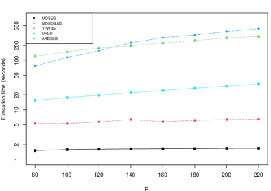
Figure 1: Execution time in seconds of MOSEG and MOSEG.MS and competing methodologies on simulated datasets ($y$-axis is in log scale for ease of comparison). Left: $p$ varies while $n=450$ is fixed. Right: $n$ varies while $p=100$ is fixed. For each setting, $100$ realisations are generated and the average execution time is reported. See Section 4.2 for full details.

Against the above literature background, we list the contributions made in this paper by proposing computationally and statistically efficient data segmentation methods.

1. Computational efficiency. For the data segmentation problem under (5), often the computational bottleneck is the local estimation of the regression parameters via penalised $M$-estimation such as Lasso. We propose MOSEG, a moving window-based two-stage methodology, and its multiscale extension, which are both highly efficient computationally. In the first stage, MOSEG scans the data for multiple change points using a moving window of length $G$ on a coarse grid of size $O(nG^{-1})$, which is followed by a simple location refinement step minimising the local residual sum of squares. The adoption of a coarse grid in the first stage contributes greatly to the reduction of Lasso estimation steps while losing little detection power. Figure 1 demonstrates the computational competitiveness of the proposed MOSEG and MOSEG.MS where they greatly outperform the existing methodologies in their execution time for a range of $n$ and $p$.

2. Multiscale change point detection. We propose a multiscale extension of the single-bandwidth methodology MOSEG. Referred to as MOSEG.MS, it is fully adaptive to the difficult scenarios with multiscale change points, where large frequent parameter shifts and small changes over long stretches of stationarity are simultaneously present, while still enjoying computational competitiveness. To the best of our knowledge, MOSEG.MS is the only data segmentation methodology under the model (5) for which the detection and localisation consistency is derived explicitly for the broad parameter space that permits multiscale change points. Also, while there exist several data segmentation methods that propose to apply moving window-based procedures with multiple bandwidths, MOSEG.MS is the first extension in high dimensions with a guaranteed rate of localisation.

3. Theoretical consistency in general settings. We show the consistency of MOSEG and MOSEG.MS in estimating the total number and the locations of multiple change points. Under Gaussianity, their separation and localisation rates nearly match the minimax lower bounds up to a logarithmic factor. Moreover, in our theoretical investigation, we permit temporal dependence as well as tail behaviour heavier than sub-Gaussianity. This, compared to the existing literature where independence and (sub-)Gaussianity assumptions are commonly made, shows that the proposed methods work well in situations that are more realistic for empirical applications.

The rest of the paper is organised as follows. Section 2 introduces MOSEG, the single-bandwidth methodology, and establishes its theoretical consistency. Then in Section 3, we propose its multiscale extension, MOSEG.MS, and show that it achieves theoretical consistency in a broader parameter space. Numerical experiments in Section 4 demonstrate the competitiveness of the proposed methods in comparison with the existing data segmentation algorithms and Section 5 provides a real data application to equity premium data. In the Appendix, we provide a comprehensive comparison between the existing methods and MOSEG and MOSEG.MS both on their theoretical and computational properties, and present all the proofs and additional numerical results. The R software implementing MOSEG and MOSEG.MS is available from https://github.com/Dom-Owens-UoB/moseg.

Notation.

For a random variable $X$, we write $\|X\|_{\nu}=[\mathsf{E}(|X|^{\nu})]^{1/\nu}$ for $\nu>0$. For $\mathbf{a}=(a_{1},\ldots,a_{p})^{\top}\in\mathbb{R}^{p}$, we write $\text{supp}(\mathbf{a})=\{i,\,1\leq i\leq p:\,a_{i}\neq 0\}$, $\left|\mathbf{a}\right|_{0}=\sum_{i=1}^{p}\mathbb{I}_{\{a_{i}\neq 0\}}$, $\left|\mathbf{a}\right|_{1}=\sum_{i=1}^{p}\left|a_{i}\right|$, $\left|\mathbf{a}\right|_{2}=(\sum_{i=1}^{p}a_{i}^{2})^{1/2}$ and $\left|\mathbf{a}\right|_{\infty}=\max_{1\leq i\leq p}\left|a_{i}\right|$. For a square matrix $\mathbf{A}$, let $\Lambda_{\max}(\mathbf{A})$ and $\Lambda_{\min}\left(\mathbf{A}\right)$ denote its maximum and minimum eigenvalues, respectively. For a set $\mathcal{A}$, we denote its cardinality by $\left|\mathcal{A}\right|$. For sequences of positive numbers $\{a_{n}\}$ and $\{b_{n}\}$, we write $a_{n}\lesssim b_{n}$ if there exists some constant $C>0$ such that $a_{n}/b_{n}\leq C$ as $n\to\infty$. Finally, we write $a\vee b=\max(a,b)$ and $a\wedge b=\min(a,b)$.

2 Single-bandwidth methodology

We introduce MOSEG, a single-bandwidth two-stage methodology for data segmentation in regression settings. We first describe its two stages in Section 2.1, establish its theoretical consistency in Section 2.2 and verify meta-assumptions made for the theoretical analysis in Section 2.3 for a class of linear processes with serial dependence and heavier tails than that permitted under sub-Gaussianity.

2.1 MOSEG

2.1.1 Stage 1: Moving window procedure on a coarse grid

Single-bandwidth moving window procedures have successfully been adopted for univariate (Preuss et al.,, 2015; Yau and Zhao,, 2016; Eichinger and Kirch,, 2018), multivariate (Kirch and Reckrühm,, 2022) and high-dimensional (Cho et al.,, 2023) time series segmentation. When applying a moving window-based procedure to a data segmentation problem, the key challenge is to carefully design a detector statistic which, when adopted for scanning the data for changes, has good detection power against the type of changes which is of interest to detect.

For a given bandwidth $G\in\mathbb{N}$ satisfying $G\leq n/2$, our proposed detector statistic is

$$T_{k}(G)=\sqrt{\frac{G}{2}}\left|\widehat{\bm{\beta}}_{k,k+G}-\widehat{\bm{\beta}}_{k-G,k}\right|_{2},\quad G\leq k\leq n-G.$$ (6)

Here, $\widehat{\bm{\beta}}_{s,e}$ denotes an estimator of the vector of parameters obtained from $(Y_{t},\mathbf{x}_{t}),\,s+1\leq t\leq e$, for any $0\leq s<e\leq n$. The statistic $T_{k}(G)$ contrasts the local parameter estimators from two adjacent data sections over $\{k-G+1,\ldots,k\}$ and $\{k+1,\ldots,k+G\}$. Then, $T_{k}(G)$ is expected to form local maxima near the change points where the local parameter estimators differ the most, and thus it is well-suited for detecting and locating the change points under the model (5).

We propose to obtain the local estimator $\widehat{\bm{\beta}}_{s,e}$ via Lasso, as

$$\widehat{\bm{\beta}}_{s,e}(\lambda)={\arg\min}_{\bm{\beta}\in\mathbb{R}^{p}}\sum_{t=s+1}^{e}(Y_{t}-\mathbf{x}_{t}^{\top}\bm{\beta})^{2}+\lambda\sqrt{e-s}|\bm{\beta}|_{1}$$ (7)

for some tuning parameter $\lambda>0$. In what follows, we suppress the dependence of this estimator on $\lambda$ when there is no confusion. The estimand of $\widehat{\bm{\beta}}_{k-G,k}$ is

$$\bm{\beta}^{*}_{k-G,k}=\frac{1}{G}\sum_{j=L(k-G+1)}^{L(k)}\left\{(\theta_{j+1}\wedge k)-((k-G)\vee\theta_{j})\right\}\bm{\beta}_{j},$$ (8)

where $L(t)=\{j,\,0\leq j\leq q:\,\theta_{j}+1\leq t\}$ denotes the index of a change point $\theta_{j}$ that is the closest to $t$ while lying strictly to its left. In short, $\bm{\beta}^{*}_{k-G,k}$ is a weighted sum of $\bm{\beta}_{j}$ with the weights corresponding to the proportion of the intervals $\{k-G+1,\ldots,k\}$ overlapping with $\{\theta_{j}+1,\ldots,\theta_{j+1}\}$.

Scanning the detector statistic $T_{k}(G)$ over all $k\in\{G,\ldots,n-G\}$ requires the computation of the Lasso estimator $O(n)$ times. This is far fewer than $O(n^{2})$ times required by dynamic programming algorithms for $\ell_{0}$-penalised cost minimisation (Rinaldo et al.,, 2021; Xu et al.,, 2022), but it may still pose a computational bottleneck when the data sequence is very long or its dimensionality ultra high. Instead, we propose to evaluate $T_{k}(G)$ on a coarser grid only for generating pre-estimators of the change points. Let $\mathcal{T}$ denote the grid over which we evaluate $T_{k}(G)$, which is given by

$$\mathcal{T}=\mathcal{T}(r,G)=\left\{G+\lfloor rG\rfloor m,\,0\leq m\leq\left\lfloor\frac{n-2G}{rG}\right\rfloor\right\}$$ (9)

with some constant $r\in[G^{-1},1)$ that controls the coarseness of the grid. When $r=G^{-1}$, we have the finest grid $\mathcal{T}=\{G,\ldots,n-G\}$ and the grid becomes coarser with increasing $r$.

Motivated by Eichinger and Kirch, (2018), who considered the problem of detecting multiple shifts in the mean of univariate time series using a moving window procedure, we propose to accept all significant local maximisers of $T_{k}(G)$ over $k\in\mathcal{T}$ as the pre-estimators of the change points. That is, for some threshold $D>0$ and a tuning parameter $\eta\in(0,1]$, we accept all $\widetilde{\theta}\in\mathcal{T}$ that simultaneously satisfy

$$T_{\widetilde{\theta}}(G)>D\quad\text{and}\quad\widetilde{\theta}={\arg\max}_{k\in\mathcal{T}:\,|k-\widetilde{\theta}|\leq\eta G}\,T_{k}(G).$$ (10)

That is, at such $\widetilde{\theta}$, the detector $T_{\widetilde{\theta}}(G)$ exceeds the threshold and attains a local maximum over the grid within the interval of length $\eta G$. We denote the set collecting all pre-estimators fulfilling (10), by $\widetilde{\Theta}=\{\widetilde{\theta}_{j},\,1\leq j\leq\widehat{q}:\,\widetilde{\theta}_{1}<\ldots<\widetilde{\theta}_{\widehat{q}}\}$ with $\widehat{q}=|\widetilde{\Theta}|$ as the estimator of the number of change points. This grid-based approach substantially reduces the computational complexity by requiring the Lasso estimators to be computed only $O(n/\lfloor rG\rfloor)$ times. Even so, it is sufficient for detecting the presence of all $q$ change points, provided that $r$ is chosen not too large (see Theorem 1 (i) below). We remark that the idea of utilising only a sub-sample of the data for detecting the presence of change points, has been proposed for handling long data sequences in the context of univariate mean change point detection (Lu et al.,, 2017). The next section describes the location refinement step applied to the pre-estimators of change point locations.

2.1.2 Stage 2: Location refinement

Once the set of pre-estimators $\widetilde{\Theta}$ is generated by the first-stage moving window procedure on a coarse grid, we further refine the location estimators. It involves the local evaluation and minimisation of the following objective function

$$Q\left(k;a,b,\widehat{\bm{\gamma}}^{\text{\tiny L}},\widehat{\bm{\gamma}}^{\text{\tiny R}}\right)=\sum_{t=a+1}^{k}(Y_{t}-\mathbf{x}_{t}^{\top}\widehat{\bm{\gamma}}^{\text{\tiny L}})^{2}+\sum_{t=k+1}^{b}(Y_{t}-\mathbf{x}_{t}^{\top}\widehat{\bm{\gamma}}^{\text{\tiny R}})^{2}\text{ for }k=a+1,\ldots,b,$$ (11)

for suitably chosen $a$, $b$, $\widehat{\bm{\gamma}}^{\text{\tiny L}}$ and $\widehat{\bm{\gamma}}^{\text{\tiny R}}$.

For each $j=1,\ldots,\widehat{q}$, let $\widetilde{\theta}_{j}^{\text{\tiny L}}=\widetilde{\theta}_{j}-\lfloor G/2\rfloor$ and $\widetilde{\theta}_{j}^{\text{\tiny R}}=\widetilde{\theta}_{j}+\lfloor G/2\rfloor$, and consider the following local parameter estimators

$$\widehat{\bm{\beta}}^{\text{\tiny L}}_{j}=\widehat{\bm{\beta}}_{0\vee(\widetilde{\theta}_{j}^{\text{\tiny L}}-G),\widetilde{\theta}_{j}^{\text{\tiny L}}}\quad\text{and}\quad\widehat{\bm{\beta}}^{\text{\tiny R}}_{j}=\widehat{\bm{\beta}}_{\widetilde{\theta}_{j}^{\text{\tiny R}},(\widetilde{\theta}_{j}^{\text{\tiny R}}+G)\wedge n},$$ (12)

which serve as the estimators of $\bm{\beta}_{j-1}$ and $\bm{\beta}_{j}$, respectively. Then in Stage 2, we propose to obtain a refined location estimator of $\theta_{j}$ from its pre-estimator $\widetilde{\theta}_{j}$, as

$$\widehat{\theta}_{j}={\arg\min}_{\widetilde{\theta}_{j}-G+1\leq k\leq\widetilde{\theta}_{j}+G}\,Q\left(k;\widetilde{\theta}_{j}-G,\widetilde{\theta}_{j}+G,\widehat{\bm{\beta}}^{\text{\tiny L}}_{j},\widehat{\bm{\beta}}^{\text{\tiny R}}_{j}\right),$$ (13)

for all $j=1,\ldots,\widehat{q}$. A similar approach has commonly been taken in the change point literature, see e.g. Kaul et al., 2019b and Xu et al., (2022) for the data segmentation problem under the model (5). Our proposal differs from theirs only in that the interval over which the search is performed in (13), is chosen to contain exactly one change point with high probability under Assumption 5 (a) below. Referring to the methodology combining the two stages as MOSEG, we provide its algorithmic description in Algorithm 1 of Appendix D.

2.2 Consistency of MOSEG

We make the following assumptions on $(\mathbf{x}_{t},\varepsilon_{t}),\,1\leq t\leq n$.

Assumption 1.

We assume that $\mathsf{E}(\mathbf{x}_{t})=\mathbf{0}$, $\mathsf{E}(\varepsilon_{t})=0$ and $\mathsf{Var}(\varepsilon_{t})=\sigma_{\varepsilon}^{2}$ for all $t=1,\ldots,n$, and that $\mathsf{Cov}(\mathbf{x}_{t})=\bm{\Sigma}_{x}$ has its eigenvalues bounded, i.e. there exist $0\leq\omega\leq\bar{\omega}<\infty$ such that

$$\omega\leq\Lambda_{\min}(\bm{\Sigma}_{x})\leq\Lambda_{\max}(\bm{\Sigma}_{x})\leq\bar{\omega}.$$

The condition on the eigenvalues of $\bm{\Sigma}_{x}$ can also be found e.g. in Rinaldo et al., (2021) and Wang et al., (2019). Where relevant, we explicitly specify the roles played by $\omega$ and $\bar{\omega}$ in presenting the theoretical results, which indicates how this condition may be relaxed. Assumptions 2 and 3 below extend the deviation bound and restricted eigenvalue (RE) conditions required for high-dimensional $M$-estimation (van de Geer and Bühlmann,, 2009; Loh and Wainwright,, 2012; Negahban et al.,, 2012), to change point settings. We later verify the assumptions under general conditions accommodating serial dependence as well as non-Gaussian tail behaviour. Here, we explicitly state these meta-assumptions to highlight the full generality of the consistency of MOSEG derived in this section.

Assumption 2 (Deviation bound).

There exist fixed constants $C_{0},C_{\text{\tiny dev}}>0$ and some $\rho_{n,p}~{}\to~{}\infty$ as $n,p\to\infty$, such that $\mathsf{P}(\mathcal{D}^{(1)}\cap\mathcal{D}^{(2)})\to 1$, where

$$\mathcal{D}^{(1)} =\left\{\max_{0\leq s<e\leq n,\,e-s\geq C_{0}\rho^{2}_{n,p}}\left|\frac{1}{\sqrt{e-s}}\sum_{t=s+1}^{e}\varepsilon_{t}\mathbf{x}_{t}\right|_{\infty}\leq C_{\text{\tiny dev}}\rho_{n,p}\right\},$$

$$\mathcal{D}^{(2)} =\left\{\max_{\begin{subarray}{c}0\leq s<e\leq n,\,e-s\geq C_{0}\rho^{2}_{n,p}\\ |\{s+1,\ldots,e\}\cap\Theta|\leq 1\end{subarray}}\left|\frac{1}{\sqrt{e-s}}\sum_{t=s+1}^{e}(Y_{t}-\mathbf{x}_{t}^{\top}\bm{\beta}^{*}_{s,e})\mathbf{x}_{t}\right|_{\infty}\leq C_{\text{\tiny dev}}\rho_{n,p}\right\}.$$

Assumption 3 (Restricted eigenvalue).

There exist fixed constants $C_{\text{\tiny RE}}>0$ and $\tau\in[0,1)$ such that $\mathsf{P}(\mathcal{R}^{(1)}\cap\mathcal{R}^{(2)})\to~{}1$, where

$$\mathcal{R}^{(1)} =\left\{\sum_{t=s+1}^{e}\mathbf{a}^{\top}\mathbf{x}_{t}\mathbf{x}_{t}^{\top}\mathbf{a}\geq(e-s)\omega|\mathbf{a}|_{2}^{2}-C_{\text{\tiny RE}}\log(p)(e-s)^{\tau}|\mathbf{a}|_{1}^{2}\text{ for all }\right.$$

$$\qquad\left.0\leq s<e\leq n\text{ satisfying }e-s\geq C_{0}\rho^{2}_{n,p}\text{ and }\mathbf{a}\in\mathbb{R}^{p}\right\},$$

$$\mathcal{R}^{(2)} =\left\{\sum_{t=s+1}^{e}\mathbf{a}^{\top}\mathbf{x}_{t}\mathbf{x}_{t}^{\top}\mathbf{a}\leq(e-s)\bar{\omega}|\mathbf{a}|_{2}^{2}+C_{\text{\tiny RE}}\log(p)(e-s)^{\tau}|\mathbf{a}|_{1}^{2}\text{ for all }\right.$$

$$\qquad\left.0\leq s<e\leq n\text{ satisfying }e-s\geq C_{0}\rho^{2}_{n,p}\text{ and }\mathbf{a}\in\mathbb{R}^{p}\right\}.$$

For each $j=0,\ldots,q$, we denote by $\mathcal{S}_{j}=\text{supp}(\bm{\beta}_{j})$ the support of $\bm{\beta}_{j}$, and by $\mathfrak{s}=\max_{0\leq j\leq q}|\mathcal{S}_{j}|$ the maximum segment-wise sparsity of the regression parameters. We make the following assumptions on the size of change $\delta_{j}=|\bm{\beta}_{j}-\bm{\beta}_{j-1}|_{2}$ and the spacing between the neighbouring change points.

Assumption 4.

There exists some constant $C_{\delta}>0$ such that $\max_{1\leq j\leq q}\delta_{j}\leq C_{\delta}$.

Assumption 4 is a technical condition under which we focus on the more challenging regime where the size of change is allowed to tend to zero; an analogous condition is found in Lee et al., (2016), Kaul et al., 2019b , Wang et al., (2021) and Xu et al., (2022). It follows immediately if we assume that $\mathsf{Var}(Y_{t})<\infty$, since $\mathsf{Var}(Y_{t})\geq\omega\sum_{j=0}^{q}|\bm{\beta}_{j}|_{2}^{2}\cdot\mathbb{I}_{\{\theta_{j}+1\leq t\leq\theta_{j}\}}+\sigma_{\varepsilon}^{2}$. Without Assumption 4, it incurs an extra multiplicative factor $\mathfrak{s}$ in the detection boundary (see Assumption 5 (b) below) and the rate of localisation, see also Rinaldo et al., (2021).

Assumption 5.

The bandwidth $G$ fulfils the following conditions with $\tau$, $\rho_{n,p}$ and $\omega$ introduced in Assumptions 1, 2 and 3.

1. $2G\leq\min_{1\leq j\leq q+1}(\theta_{j}-\theta_{j-1})$.

2. There exists a fixed constant $C_{1}>0$ such that

   $$\min_{1\leq j\leq q}\delta_{j}^{2}G\geq C_{1}\max\left\{\omega^{-2}\mathfrak{s}\rho_{n,p}^{2},\left(\omega^{-1}\mathfrak{s}\log(p)\right)^{1/(1-\tau)}\right\}.$$

Assumption 5 (a) relates the choice of bandwidth $G$ to the minimum spacing between the change points. Together, (a) and (b) specify the separation rate imposing a lower bound on

$$\Delta^{(1)}=\min_{1\leq j\leq q}\delta_{j}^{2}\cdot\min_{0\leq j\leq q}(\theta_{j+1}-\theta_{j}),$$ (14)

for all the $q$ change points to be detectable by MOSEG. Later in Section 3, we propose a multiscale extension of MOSEG which achieves consistency under a more relaxed condition than Assumption 5.

Theorem 1.

Suppose that Assumptions 1, 2, 3, 4 and 5 hold. Let the tuning parameters satisfy $\lambda\geq 4C_{\text{\tiny dev}}\rho_{n,p}$, $r\in[1/G,1/4)$, $\eta\in(4r,1]$ and

$$\frac{48\sqrt{\mathfrak{s}}\lambda}{\omega}<D<\frac{\eta}{4\sqrt{2}}\min_{1\leq j\leq q}\delta_{j}\sqrt{G}.$$ (15)

Then conditional on $\mathcal{D}^{(1)}\cap\mathcal{D}^{(2)}\cap\mathcal{R}^{(1)}\cap\mathcal{R}^{(2)}$, the following holds.

1. Stage 1 of MOSEG returns $\widetilde{\Theta}=\{\widetilde{\theta}_{j},\,1\leq j\leq\widehat{q}:\,\widetilde{\theta}_{1}<\ldots<\widetilde{\theta}_{\widehat{q}}\}$ which satisfies

   $$\widehat{q}=q\quad\text{and}\quad|\widetilde{\theta}_{j}-\theta_{j}|\leq\frac{48\sqrt{2\mathfrak{s}G}\lambda}{\omega\delta_{j}}+\lfloor rG\rfloor<\left\lfloor\frac{G}{2}\right\rfloor\text{ for each $j=1,\ldots,q$.}$$

2. There exists a large enough constant $c_{0}>0$ such that Stage 2 of MOSEG returns $\widehat{\Theta}=\{\widehat{\theta}_{j},\,1\leq j\leq\widehat{q}:\,\widehat{\theta}_{1}<\ldots<\widehat{\theta}_{\widehat{q}}\}$ which satisfies

   $$\max_{1\leq j\leq q}\delta_{j}^{2}|\widehat{\theta}_{j}-\theta_{j}|\leq c_{0}\max\left(\mathfrak{s}\rho_{n,p}^{2},\left(\mathfrak{s}\log(p)\right)^{\frac{1}{1-\tau}}\right).$$

Theorem 1 (i) establishes that Stage 1 of MOSEG correctly estimates the number of change points as well as identifying their locations by the pre-estimators with some accuracy. There is a trade-off between computational efficiency and theoretical consistency with respect to the choice of $r$. On one hand, increasing $r$ leads to a coarser grid $\mathcal{T}$ with its cardinality $|\mathcal{T}|=O(n/(rG))$, and thus reduces the computational cost. On the other, the pre-estimators lie in the grid such that the best approximation to each change point $\theta_{j}$ can be as far from $\theta_{j}$ as $\lfloor rG\rfloor/2$, which is reflected on the localisation property of the pre-estimators.

Theorem 1 (ii) derives the rate of estimation for the second-stage estimators $\widehat{\theta}_{j}$ which shows that the location estimation is more challenging when the size of change $\delta_{j}$ is small. Note that we always have $\max_{1\leq j\leq q}\delta_{j}^{-2}\max(\mathfrak{s}\rho_{n,p}^{2},(\mathfrak{s}\log(p))^{1/(1-\tau)})\lesssim G\lesssim\min_{1\leq j\leq q+1}(\theta_{j}-\theta_{j-1})$ under Assumption 4. In Section 2.3, we consider two scenarios permitting temporal dependence and non-Gaussianity on $(\mathbf{x}_{t},\varepsilon_{t})$, and give concrete rates in place of $\rho_{n,p}$ and $\tau$. In particular, as shown in Corollary 3 (ii), the rate derived in Theorem 1 (ii) is near-minimax optimal under Gaussianity.

2.3 Verification of Assumptions 2 and 3

Assumptions 2 and 3 generalise the deviation bound and restricted eigenvalue conditions which are often found in the high-dimensional $M$-estimation literature, to accommodate change points, serial dependence and heavy-tailedness. Condition 1 gives instances of $\{(\mathbf{x}_{t},\varepsilon_{t})\}_{t=1}^{n}$ that fulfil Assumptions 2 and 3 and specify the corresponding $\rho_{n,p}$ and $\tau$.

Condition 1.

Suppose that for i.i.d. random vectors $\bm{\xi}_{t}=(\xi_{1t},\ldots,\xi_{p+1,t})^{\top}\in\mathbb{R}^{p+1},\,t\in\mathbb{Z}$, with $\mathsf{E}(\bm{\xi}_{t})=\mathbf{0}$ and $\mathsf{Cov}(\bm{\xi}_{t})=\mathbf{I}$, we have

$$\begin{bmatrix}\mathbf{x}_{t}\\ \varepsilon_{t}\end{bmatrix} =\sum_{\ell=0}^{\infty}\mathbf{D}_{\ell}\bm{\xi}_{t-\ell}\quad\text{with}\quad\mathbf{D}_{\ell}=[D_{\ell,ik},\,1\leq i,k\leq p+1]\in\mathbb{R}^{(p+1)\times(p+1)}$$ (16)

subject to $\mathsf{E}(\mathbf{x}_{t}\varepsilon_{t})=\mathbf{0}$. Further, there exist constants $\Xi>0$ and $\varsigma>2$ such that

$$|D_{\ell,ik}|\leq C_{ik}(1+\ell)^{-\varsigma}\quad\text{with}\quad\max\left\{\max_{1\leq k\leq p+1}\sum_{i=1}^{p+1}C_{ik},\,\max_{1\leq i\leq p+1}\sum_{k=1}^{p+1}C_{ik}\right\}\leq\Xi$$ (17)

for all $\ell\geq 0$. Finally, we impose either of the two conditions on $\xi_{it}$.

1. There exist some constants $C_{\xi}>0$ and $\gamma\in(0,2]$ such that $(\mathsf{E}(|\xi_{it}|^{\nu}))^{1/\nu}=\|\xi_{it}\|_{\nu}\leq C_{\xi}\nu^{\gamma}$ for all $\nu\geq 1$. In other words, $\|\xi_{it}\|_{\psi_{\nu}}:=\sup_{\nu\geq 1}\nu^{-1/\gamma}\|\xi_{it}\|_{\nu}\leq C_{\xi}$.

2. $\xi_{it}\sim_{\text{iid}}\mathcal{N}(0,1)$.

Proposition 2.

Suppose that Assumptions 1 and 4 and Condition 1 hold. Then, there exist some constants $c_{1},c_{2}>0$ such that $\mathsf{P}(\mathcal{D}^{(1)}\cap\mathcal{D}^{(2)}\cap\mathcal{R}^{(1)}\cap\mathcal{R}^{(2)})\geq 1-c_{1}(p\vee n)^{-c_{2}}$, with $\omega=\Lambda_{\min}(\bm{\Sigma}_{x})/2$, $\bar{\omega}=3\Lambda_{\max}(\bm{\Sigma}_{x})/2$, and $\tau$ and $\rho_{n,p}$ chosen as below.

1. Under Condition 1 (a), we set $\tau=(4\gamma+2)/(4\gamma+3)$ and $\rho_{n,p}=\log^{2\gamma+3/2}(p\vee n)$.

2. Under Condition 1 (b), we set $\tau=0$ and $\rho_{n,p}=\sqrt{\log(p\vee n)}$.

Under Condition 1, $\{(\mathbf{x}_{t},\varepsilon_{t})\}_{t=1}^{n}$ is a linear process with algebraically decaying serial dependence. Also, Condition 1 (a) permits heavier tail behaviour than that allowed under sub-Gaussianity or sub-exponential distributions when $\gamma>1/2$ and $\gamma>1$, respectively.

Remark 1.

In the change point literature, Wang and Zhao, (2022) propose a change point test and investigate its properties under $\beta$-mixing, and Xu et al., (2022) analyse the $\ell_{0}$-penalised least squares estimation approach when the functional dependence of $\{\mathbf{x}_{t}\}_{t=1}^{n}$ and $\{\varepsilon_{t}\}_{t=1}^{n}$ decays exponentially. Relaxing the Gaussianity, it is typically required that $\mathbf{x}_{t}$ is a sub-Weibull random vector, i.e. $\sup_{\mathbf{a}\in\mathbb{B}_{2}(1)}\|\mathbf{a}^{\top}\mathbf{x}_{t}\|_{\psi_{\nu}}<\infty$ for some $\gamma>0$ (where $\mathbb{B}_{d}(r)=\{\mathbf{a}:\,|\mathbf{a}|_{d}\leq r\}$) and similarly, $\|\varepsilon_{t}\|_{\psi_{\gamma}}<\infty$. Under these assumptions, the common approach is to verify the deviation bound and restricted eigenvalue conditions analogous to those made in Assumptions 2–3, with which the uniform consistency of the local Lasso estimators is derived. Instead, we explicitly state the meta-assumptions to highlight that the proposed MOSEG achieves consistency whenever Assumptions 2–3 are met. These in turn can be shown to hold in settings beyond those considered in Condition 1 by using the arguments adopted in the literature establishing the consistency of Lasso-type estimator (when $q=0$) under a variety of characterisations of serial dependence and non-Gaussianity (Wu and Wu,, 2016; Adamek et al.,, 2020; Han and Tsay,, 2020; Wong et al.,, 2020).

Corollary 3 follows immediately from Theorem 1 and Proposition 2.

Corollary 3.

Suppose that Assumptions 1, 4 and 5 and Condition 1 hold, and $\lambda$, $r$, $\eta$ and $D$ are chosen as in Theorem 1. Then, there exist constants $c_{i}>0,\,i=0,1,2$, such that $\widehat{\Theta}=\{\widehat{\theta}_{j},\,1\leq j\leq\widehat{q}:\,\widehat{\theta}_{1}<\ldots<\widehat{\theta}_{\widehat{q}}\}$ returned by MOSEG satisfies the following.

1. Under Condition 1 (a), we have

   $$\mathsf{P}\left(\widehat{q}=q\text{ \ and \ }\max_{1\leq j\leq q}\delta_{j}^{2}|\widehat{\theta}_{j}-\theta_{j}|\leq c_{0}\left(\mathfrak{s}\log(p\vee n)\right)^{4\gamma+3}\right)\geq 1-c_{1}(p\vee n)^{-c_{2}}.$$

2. Under Condition 1 (b), we have

   $$\mathsf{P}\left(\widehat{q}=q\text{ \ and \ }\max_{1\leq j\leq q}\delta_{j}^{2}|\widehat{\theta}_{j}-\theta_{j}|\leq c_{0}\mathfrak{s}\log(p\vee n)\right)\geq 1-c_{1}(p\vee n)^{-c_{2}}.$$

Corollary 3 (ii) shows that under Gaussianity, the rate of localisation attained by MOSEG matches the minimax lower bound up to $\log(p\vee n)$, see Lemma 4 of Rinaldo et al., (2021). At the same time, Assumption 5 (b) translates to $\Delta^{(1)}\gtrsim\mathfrak{s}\log(p\vee n)$ in this setting, nearly matching the minimax lower bound on the separation rate derived in Lemma 3 of Rinaldo et al., (2021) up to the logarithmic term. We refer to Appendix A for comprehensive comparison between MOSEG, its multiscale extension to be introduced in Section 3, and the existing methods for the change point detection problem under (5), on their theoretical and computational properties.

3 Multiscale methodology

The single-bandwidth methodology proposed in Section 2 enjoys theoretical consistency as well as computational efficiency, but faces the difficulty arising from identifying a bandwidth that satisfies Assumption 5 (a)–(b) simultaneously. In this section, we propose MOSEG.MS, a multiscale extension of MOSEG, and show that it achieves consistency in a parameter space broader than that allowed by Assumption 5.

3.1 MOSEG.MS: Multiscale extension of MOSEG

Similarly to MOSEG, MOSEG.MS consists of moving window-based data scanning and location refinement steps but it takes a set of bandwidths as an input. The key innovation lies in that for each change point, MOSEG.MS learns the bandwidth best-suited for its detection and localisation from the given set of bandwidths. While there exist multiscale extensions of moving sum procedures, they are mostly developed for univariate time series segmentation (Messer et al.,, 2014; Cho and Kirch, 2021b, ) and to the best of our knowledge, this is a first attempt at rigorously studying such an extension in a high-dimensional setting.

Below we describe MOSEG.MS step-by-step. An algorithmic description of MOSEG.MS is given in Algorithm 2 of Appendix D.

Step 1: Pre-estimator generation.

Given a set of bandwidths $\mathcal{G}=\{G_{h},\,1\leq h\leq H:\,G_{1}<\ldots<G_{H}\}$, we generate the coarse grid associated with each $G_{h}$ and the parameter $r$ by $\mathcal{T}_{h}=\mathcal{T}(r,G_{h})$, see (9). As in Stage 1 of MOSEG, the sets of pre-estimators $\widetilde{\Theta}(G_{h})$ are generated for $h=1,\ldots,H$, and we denote by $\widetilde{\Theta}(\mathcal{G})=\cup_{h=1}^{H}\widetilde{\Theta}(G_{h})$ the pooled set of all such pre-estimators. By (10), at each $\widetilde{\theta}\in\widetilde{\Theta}(G_{h})$, we have $T_{\widetilde{\theta}}(G_{h})>D$ and $\widetilde{\theta}=\arg\max_{k\in\mathcal{I}_{\eta}(\widetilde{\theta})\cap\mathcal{T}_{h}}T_{k}(G_{h})$, where $\mathcal{I}_{\eta}(\widetilde{\theta})=\{\widetilde{\theta}-\lfloor\eta G_{h}\rfloor+1,\ldots,\widetilde{\theta}+\lfloor\eta G_{h}\rfloor\}$ denotes the detection interval associated with $\widetilde{\theta}$. For simplicity, we write $\mathcal{I}_{1}(\widetilde{\theta})=\mathcal{I}(\widetilde{\theta})$. Below, we sometimes write $\widetilde{\theta}(G)\in\widetilde{\Theta}(G)$ to highlight that the pre-estimator is obtained with the bandwidth $G$, and denote by $G(\widetilde{\theta})$ the bandwidth involved in the detection of a pre-estimator $\widetilde{\theta}$. If some $\widetilde{\theta}$ is detected with more than one bandwidths, we distinguish between them.

Step 2: Anchor estimator identification.

Next, we identify anchor change point estimators $\widetilde{\theta}^{A}(G)\in\widetilde{\Theta}(\mathcal{G})$ detected at some $G\in\mathcal{G}$ which satisfy

$$\bigcup_{h:\,G_{h}<G}\,\bigcup_{k\in\widetilde{\Theta}(G_{h})}\left\{\mathcal{I}(k)\cap\mathcal{I}(\widetilde{\theta}^{A}(G))\right\}=\emptyset.$$ (18)

That is, each anchor change point estimator does not have its detection interval overlap with the detection interval of any pre-estimator that is detected with a finer bandwidth. Denote the set of all such anchor change point estimators by $\widetilde{\Theta}^{A}=\{\widetilde{\theta}^{A}_{j},\,1\leq j\leq\widehat{q}:\,\widetilde{\theta}^{A}_{1}<\ldots<\widetilde{\theta}^{A}_{\widehat{q}}\}$, with $\widehat{q}=|\widetilde{\Theta}^{A}|$ as an estimator of the number of change points $q$.

Step 3: Pre-estimator clustering.

We find subsets of the pre-estimators in $\widetilde{\Theta}(\mathcal{G})$ denoted by $\mathcal{C}_{j},\,j=1,\ldots,\widehat{q}$, as described below. Initialised as $\mathcal{C}_{j}=\emptyset$, for each $j$, we add to $\mathcal{C}_{j}$ the $j$th anchor estimator $\widetilde{\theta}^{A}_{j}$ as well as all $\widetilde{\theta}\in\widetilde{\Theta}(\mathcal{G})$ which simultaneously fulfil

$$\mathcal{I}(\widetilde{\theta})\cap\mathcal{I}(\widetilde{\theta}^{A}_{j})\neq\emptyset,\quad\text{and}$$

$$\{\widetilde{\theta}-G(\widetilde{\theta})-\lfloor G(\widetilde{\theta})/2\rfloor+1,\ldots,\widetilde{\theta}+G(\widetilde{\theta})+\lfloor G(\widetilde{\theta})/2\rfloor\}\cap\mathcal{I}(\widetilde{\theta}^{A}_{j^{\prime}})=\emptyset\text{ for all }j^{\prime}\neq j.$$ (19)

It is possible that some pre-estimators do not belong to any of $\mathcal{C}_{j},\,1\leq j\leq\widehat{q}$, but each cluster contains at least one estimator by construction.

Step 4: Location refinement.

For each $\mathcal{C}_{j},\,j=1,\ldots,\widehat{q}$, we denote the smallest and the largest bandwidths associated with the detection of the pre-estimators in $\mathcal{C}_{j}$, by $G^{m}_{j}$ and $G^{M}_{j}$, respectively, and the corresponding pre-estimators by $\widetilde{\theta}^{m}_{j}$ and $\widetilde{\theta}^{M}_{j}$ (when $|\mathcal{C}_{j}|=1$, we have $\widetilde{\theta}^{m}_{j}=\widetilde{\theta}^{M}_{j}=\widehat{\theta}^{A}_{j}$ and $G^{m}_{j}=G^{M}_{j}$). Setting $G^{*}_{j}=\lfloor 3G^{m}_{j}/4+G^{M}_{j}/4\rfloor$, we identify the local minimiser of the objective function defined in (11), as

$$\check{\theta}_{j}={\arg\min}_{\widetilde{\theta}^{m}_{j}-G^{*}_{j}+1\leq k\leq\widetilde{\theta}^{m}_{j}+G^{*}_{j}}Q\left(k;\widetilde{\theta}^{m}_{j}-G^{*}_{j},\widetilde{\theta}^{m}_{j}+G^{*}_{j},\widehat{\bm{\beta}}^{\text{\tiny L}}_{j},\widehat{\bm{\beta}}^{\text{\tiny R}}_{j}\right),$$ (20)

$$\text{with}\quad\widehat{\bm{\beta}}^{\text{\tiny L}}_{j}=\widehat{\bm{\beta}}_{(\widetilde{\theta}^{m}_{j}-G^{m}_{j}-G^{*}_{j})\vee 0,\widetilde{\theta}^{m}_{j}-G^{m}_{j}}\quad\text{and}\quad\widehat{\bm{\beta}}^{\text{\tiny R}}_{j}=\widehat{\bm{\beta}}_{\widetilde{\theta}^{m}_{j}+G^{m}_{j},(\widetilde{\theta}^{m}_{j}+G^{m}_{j}+G^{*}_{j})\wedge n}.$$

Repeatedly performing (20) for $j=1,\ldots,\widehat{q}$, we obtain $\check{\Theta}=\{\check{\theta}_{j},\,1\leq j\leq\widehat{q}\}$.

The steps of MOSEG.MS algorithm have been devised to (i) group the change point estimators across multiple bandwidths, into those detecting the identical change points, and (ii) adaptively learn the bandwidth best suited to locate each change point from the bandwidths associated with the estimators in each group. For (i), we adopt the anchor estimators in Step 2 which closely resemble the final estimators produced by the bottom-up merging proposed in Messer et al., (2014) in the context of univariate data segmentation. While the merging procedure is known to achieve detection consistency, the resultant estimators do not come with a guaranteed rate of localisation. Nonetheless, they serve as an adequate ‘anchor’ for clustering the pre-estimators in Step 3. Moreover, the restriction imposed in (19) ensures that the bandwidths associated with the detection of pre-estimators clustered in $\mathcal{C}_{j}$, inform us a good choice of bandwidth for the detection of the $j$-th change point, with which we perform location refinement in Step 4.

Remark 2 (Bandwidth generation).

Cho and Kirch, 2021b propose to use $\mathcal{G}$ generated as a sequence of Fibonacci numbers, for a multiscale extension of the moving sum procedure for univariate mean change point detection (Eichinger and Kirch,, 2018). For some finest bandwidth $G_{0}=G_{1}$, we iteratively produce $G_{h},\,h\geq 2$, as $G_{h}=G_{h-1}+G_{h-2}$. Equivalently, we set $G_{h}=F_{h}G_{0}$ where $F_{h}=F_{h-1}+F_{h-2}$ with $F_{0}=F_{1}=1$. This is repeated until for some $H$, it holds that $G_{H}<\lfloor n/2\rfloor$ while $G_{H+1}\geq\lfloor n/2\rfloor$. By induction, $F_{h}=O(((1+\sqrt{2})/2)^{h})$ such that the thus-generated bandwidth set $\mathcal{G}$ satisfies $|\mathcal{G}|=O(\log(n))$.

3.2 Consistency of MOSEG.MS

We make the following assumption on the size of changes by placing a condition on

$$\Delta^{(2)}=\min_{1\leq j\leq q}\delta_{j}^{2}\cdot\min(\theta_{j+1}-\theta_{j},\theta_{j}-\theta_{j-1}).$$ (21)

Assumption 5^′.

Let $\mathcal{G}$ denote the set of bandwidths generated as in Remark 2 with $G_{1}\geq C_{0}\max\{\rho_{n,p}^{2},(\omega^{-1}\mathfrak{s}\log(p))^{1/(1-\tau)}\}$. Then, we assume that

$$\Delta^{(2)}\geq 32C_{1}\max\left\{\omega^{-2}\mathfrak{s}\rho_{n,p}^{2},\left(\omega^{-1}\mathfrak{s}\log(p)\right)^{1/(1-\tau)}\right\},$$

with $C_{1}$ from Assumption 5.

In essence, Assumption 5^′ relaxes Assumption 5 by requiring that for each $\theta_{j}$, there exists one bandwidth $G_{(j)}\in\mathcal{G}$ fulfilling the requirements imposed on a single bandwidth in the latter for all $j=1,\ldots,q$, see (a)–(b) in Appendix C.3 for further details. Compared to $\Delta^{(1)}$ defined in (14), we always have $\Delta^{(1)}\leq\Delta^{(2)}$ and, if frequent large changes and small changes over long stretches of stationarity are simultaneously present, the former can be considerably smaller than the latter (Cho and Kirch, 2021a, ). To the best of our knowledge, Theorem 4 below provides a first result obtained under the larger parameter space defined with $\Delta^{(2)}$, in establishing the consistency of a data segmentation methodology for the problem in (5). We refer to Appendix A for further discussions and comprehensive comparison between MOSEG, MOSEG.MS and competing methodologies on their theoretical properties.

Theorem 4.

Suppose that Assumptions 1, 2, 3, 4 and 5^′ hold. Let the tuning parameters satisfy $\lambda\geq 4C_{\text{\tiny dev}}\rho_{n,p}$, $r\in[G_{1}^{-1},1/4)$, $\eta\in(4r,1]$ and

$$\frac{48\sqrt{\mathfrak{s}}\lambda}{\omega}<D<{\frac{\eta}{2}\sqrt{\Delta^{(2)}}.}$$ (22)

Then, there exists a constant $c_{0}>0$ such that conditional on $\mathcal{D}^{(1)}\cap\mathcal{D}^{(2)}\cap\mathcal{R}^{(1)}\cap\mathcal{R}^{(2)}$, MOSEG.MS returns $\check{\Theta}=\{\check{\theta}_{j},\,1\leq j\leq\widehat{q}:\,\check{\theta}_{1}<\ldots<\check{\theta}_{\widehat{q}}\}$ which satisfies

$$\widehat{q}=q\quad\text{and}\quad\max_{1\leq j\leq q}\delta_{j}^{2}|\check{\theta}_{j}-\theta_{j}|\leq c_{0}\max\left(\mathfrak{s}\rho^{2}_{n,p},\left(\mathfrak{s}\log(p)\right)^{\frac{1}{1-\tau}}\right).$$

Corollary 5.

Suppose that Assumptions 1, 4 and 5^′ and Condition 1 hold, and $\lambda$, $r$ and $D$ are chosen as in Theorem 4. Then, there exist constants $c_{i}>0,\,i=0,1,2$, such that $\check{\Theta}=\{\check{\theta}_{j},\,1\leq j\leq\widehat{q}:\,\check{\theta}_{1}<\ldots<\check{\theta}_{\widehat{q}}\}$ returned by MOSEG.MS satisfies the following.

1. Under Condition 1 (a), we have

   $$\mathsf{P}\left(\widehat{q}=q\text{ \ and \ }\max_{1\leq j\leq q}\delta_{j}^{2}|\check{\theta}_{j}-\theta_{j}|\leq c_{0}\left(\mathfrak{s}\log(p\vee n)\right)^{4+3\gamma}\right)\geq 1-c_{1}(p\vee n)^{-c_{2}}.$$

2. Under Condition 1 (b), we have

   $$\mathsf{P}\left(\widehat{q}=q\text{ \ and \ }\max_{1\leq j\leq q}\delta_{j}^{2}|\check{\theta}_{j}-\theta_{j}|\leq c_{0}\mathfrak{s}\log(p\vee n)\right)\geq 1-c_{1}(p\vee n)^{-c_{2}}.$$

4 Numerical experiments

4.1 Choice of tuning parameters

We discuss the selection of tuning parameters involved in MOSEG and MOSEG.MS, namely the set of bandwidths $\mathcal{G}$, the grid $\mathcal{T}(r,G)$ in (9), $\eta\in(0,1]$ involved in the pre-estimation of the change points (see (10)), the penalty parameter $\lambda$ and the threshold $D$.

Selection of $\mathcal{G}$.

As described in Remark 2, the set of bandwidths $\mathcal{G}$ is determined once the finest bandwidth $G_{1}$ is chosen. To gain insights about the minimum bandwidth required for the reasonable performance of the local Lasso estimators, we conducted numerical experiments by simulating datasets under (5) with $q=0$, $\mathbf{x}_{t}\sim_{\text{iid}}\mathcal{N}_{p}(\mathbf{0},\mathbf{I}_{p})$, $\varepsilon_{t}\sim_{\text{iid}}\mathcal{N}(0,1)$ and $\bm{\beta}_{0}=(\beta_{0,1},\ldots,\beta_{0,p})^{\top}$ where $\beta_{0,i},\,1\leq i\leq\mathfrak{s}$, are sampled uniformly from $[-1,1]$ while $\beta_{0,i}=0,\,\mathfrak{s}+1\leq i\leq p$. Generating $100$ realisations for each setting with varying $(n,p,\mathfrak{s},G)$, we record the relative $\ell_{2}$-error $\max_{0\leq k\leq n-G}|\bm{\beta}_{0}|_{2}^{-1}|\widehat{\bm{\beta}}_{k,k+G}-\bm{\beta}_{0}|_{2}$ for each realisation. Then, we obtain a simple rule to determine the finest bandwidth as $G_{1}=G_{1}(n,p)=\lfloor c^{*}_{0}\exp(c^{*}_{1}\log\log(n)+c^{*}_{2}\log\log(p))\rfloor$ with pre-determined constants $c^{*}_{i},\,i=0,1,2$, which are chosen as transforms of the estimated regression coefficients from regressing the $90\%$-percentile of the logarithm of the estimation errors over $100$ realisations, onto the corresponding $\log(G)$, $\log\log(p)$ and $\log\log(n)$ (with $R^{2}=0.8945$). Adopting the Fibonacci sequence in Remark 2 sometimes gives a sequence of bandwidths that grows too quickly when the sample size $n$ is small. Therefore, with the finest bandwidth $G_{1}$ chosen as above, we recommend generating bandwidths as $G_{h}=\lfloor(h+2)G_{1}/3\rfloor$ for $h\geq 2$. Throughout the simulation studies and real data applications, we set $H=3$.

Selection of $D$ and $\lambda$.

Theorems 1 and 4 provide ranges of values for $\lambda$ and $D$ for theoretical consistency, but they involve unknown parameters as is typically the case in the change point literature. For their simultaneous selection, we adopt a cross validation (CV) method motivated by Zou et al., (2020). Let $\Lambda=\Lambda(G)$ denote the grid of possible values for $\lambda$ which, dependent on the bandwidth $G$, is chosen as an exponentially increasing sequence from $10^{-3}\lambda_{\max}$ up to $\lambda_{\max}$ with $\lambda_{\max}=\max_{0\leq k\leq n-G}|\sum_{t=k+1}^{k+G}\mathbf{x}_{t}Y_{t}|_{\infty}/\sqrt{G}$ the smallest value with which we obtain $\widehat{\bm{\beta}}_{k,k+G}=\mathbf{0}$ for all $0\leq k\leq n-G$. For given $G\in\mathcal{G}$ and $\lambda\in\Lambda$, we generate $\widetilde{\Theta}(G,\lambda)=\{\widetilde{\theta}_{j}(G,\lambda),\,1\leq j\leq\widetilde{q}_{0}(G,\lambda)\}$, the set of pre-estimators with $D=0$, i.e. we take all local maximisers of the MOSUM statistics according to (10); due to the detection rule, we always have $\widetilde{q}_{0}(G,\lambda)\leq n/(2\eta G)$. Sorting the elements of $\widetilde{\Theta}(G,\lambda)$ in the decreasing order of the associated MOSUM detector values, we generate a sequence of nested change point models

$$\emptyset=\widetilde{\Theta}_{[0]}(G,\lambda)\subset\widetilde{\Theta}_{[1]}(G,\lambda)\subset\ldots\subset\widetilde{\Theta}_{[\widetilde{q}_{0}(G,\lambda)]}(G,\lambda)=\widetilde{\Theta}(G,\lambda).$$

Then, using the odd-indexed observations $(Y_{t},\mathbf{x}_{t}),\,t\in\mathcal{J}_{1}=\{2t+1,\,t=0,\ldots,\lfloor(n-1)/2\rfloor\}$, we produce local estimators of the regression parameters and the even-indexed observations $(Y_{t},\mathbf{x}_{t})$, $t\in\mathcal{J}_{0}=\{1,\ldots,n\}\setminus\mathcal{J}_{1}$, is used for validation. Specifically, we evaluate $\text{CV}(G,\lambda,m)=\text{RSS}_{0}(\widetilde{\Theta}_{[m]}(G,\lambda),\lambda)$, where for any $\mathcal{L}=\{\ell_{j},\,1\leq\ell_{j}\leq L:\,0=\ell_{0}<\ell_{1}<\ldots<\ell_{L}<\ell_{L+1}=n\}$,

$$\text{RSS}_{0}(\mathcal{L},\lambda) =\sum_{j=0}^{L}\sum_{\begin{subarray}{c}t\in\mathcal{J}_{0}\cap\\ \{\ell_{j}+1,\ldots,\ell_{j+1}\}\end{subarray}}\left(Y_{t}-\mathbf{x}_{t}^{\top}\widehat{\bm{\beta}}^{(1)}_{j}(\mathcal{L},\lambda)\right)^{2}.$$

Here, $\widehat{\bm{\beta}}^{(1)}_{j}(\mathcal{L},\lambda)$ denotes the Lasso estimator obtained using $(Y_{t},\mathbf{x}_{t}),\,t\in\mathcal{J}_{1}\cap\{\ell_{j},\ldots,\ell_{j+1}\}$ with the penalty parameter $\lambda$. Then for each $G_{h}\in\mathcal{G}$, we find

$$(\lambda^{*},m^{*})={\arg\min}_{\begin{subarray}{c}(\lambda,m):\,\lambda\in\Lambda,\\ 0\leq m\leq\widetilde{q}_{0}(G_{h},\lambda)\end{subarray}}\text{CV}(G_{h},\lambda,m)$$

and obtain the set of pre-estimators $\widetilde{\Theta}(G_{h})=\widetilde{\Theta}_{[m^{*}]}(G_{h},\lambda^{*})$ using $\lambda^{*}$ and $m^{*}$. This amounts to selecting the bandwidth-dependent threshold $D$ at a value just below the $m^{*}$th largest MOSUM detector value. Such $\widetilde{\Theta}(G_{h}),\,G_{h}\in\mathcal{G}$, serve as an input to Steps 2–4 of MOSEG.MS. In all numerical experiments reported in this paper, we set $|\Lambda|=5$.

Selection of other tuning parameters.

For change point estimation, we recommend to use $\eta=0.5$ in (10) based on extensive simulations, which show that the performance of MOSEG and MOSEG.MS is not too sensitive to its choice. As noted in Section 4.2, MOSEG.MS is highly competitive computationally against the existing methods even without adopting a coarse grid. Therefore, we report the results obtained with $r=G^{-1}$ (i.e. $\mathcal{T}=\{G,\ldots,n-G\}$ in (9)) in the main text and provide the results obtained with coarser grids in Appendix B.1, where we observe that adopting a coarse grid does not undermine the performance of MOSEG provided that $r$ is sufficiently small, say $r\leq 1/5$.

4.2 Computational complexity and run time

Let $\text{Lasso}(p)$ denote the cost of solving a Lasso problem with $p$ variables. For the coordinate descent algorithm (Friedman et al.,, 2010), each complete iteration of the coordinate descent has the cost $O(p^{2})$. Then, the combined computational cost of Stages 1 and 2 of MOSEG is $O(n(rG)^{-1}\text{Lasso}(p))$, and the memory cost is $O(np)$. Similarly, with the set of bandwidths generated as described in Remark 2, the complexity of the multiscale extension MOSEG.MS is $O(n(rG_{1})^{-1}\text{Lasso}(p))$ with $G_{1}$ denoting the finest scale, which follows from that $\sum_{h=1}^{H}n/(rG_{h})\leq n/(rG_{1})\sum_{h=1}^{\infty}F_{h}^{-1}=O(n(rG_{1})^{-1})$ (see Remark 2 for the notations). For the CV outlined in Section 4.1, we generate pre-estimators and evaluate the CV objective function on a sequence of nested models for each $\lambda\in\Lambda$, which brings the computational complexity of the complete MOSEG.MS methodology to $O(|\Lambda|n(rG_{1})^{-1}\text{Lasso}(p))$.

We investigate the run time of change point detection methodologies for the problem in (5). MOSEG (with $G=\lfloor n/6\rfloor$) and MOSEG.MS are applied with the tuning parameters chosen as in Section 4.1 and the finest grid (i.e. $\mathcal{T}=\{G,\ldots,n-G\}$); we include the CV procedure in run time. For comparison, we consider VPWBS (Wang et al.,, 2021), DPDU (Xu et al.,, 2022) and ARBSEG (Kaul et al., 2019a, ) applied with the recommended tuning parameters. In particular, the default implementations of VPWBS and DPDU adopt a grid of size $3$ and $4$, respectively, for the Lasso tuning parameter while MOSEG and MOSEG.MS are applied with the grid $\Lambda$ of size $|\Lambda|=5$. We generate the data under the model (M3) described in Section 4.3 below, with $\delta=1.6$ and varying $(n,p)$.

Figure 1 reports the average execution time (in seconds) over $100$ realisations for each setting, for the five methods in consideration. Both MOSEG and MOSEG.MS take only a fraction of time taken by the competing methodologies in their computation even when we do not use the coarser grid for Stage 1, and their run time does not vary much with increasing $n$ or $p$ in the ranges considered. As expected, MOSEG is faster than MOSEG.MS but the difference in execution time is much smaller than that between MOSEG.MS and other competitors.

4.3 Simulation settings

We apply MOSEG.MS to datasets simulated with varying $(n,p,\mathfrak{s})$ and change point configurations. In each setting, we generate $\mathbf{x}_{t}$ as i.i.d. Gaussian random vectors with mean $\mathbf{0}$ and the covariance matrix $\bm{\Sigma}_{x}$ which are specified below, and $\varepsilon_{t}\sim_{\text{iid}}\mathcal{N}(0,\sigma_{\varepsilon}^{2})$; unless specified otherwise, we use $\sigma_{\varepsilon}=1$. We report the results from non-Gaussian and serially dependent data in Appendix B.2 where overall, the results are not sensitive to tail behaviour or temporal dependence. Additionally, we report the results when $p=1000$ in Appendix B.3 which, together with the experiments reported in Section 4.2, demonstrate the scalability of MOSEG.MS.

The models (M1)–(M3) below are taken from Wang et al., (2021); in (M2) where non-diagonal $\bm{\Sigma}_{x}$ is considered, we adapt their model by randomly generating the set $\mathcal{S}$ on each realisation and in (M3), we consider a broader range of values for $\delta$. In what follows, we assume that for given $\mathcal{S}\subset\{1,\ldots,p\}$ with $|\mathcal{S}|=\mathfrak{s}$, the parameter vector $\bm{\beta}_{0}=(\beta_{0,1},\ldots,\beta_{0,p})^{\top}$ has $\beta_{0,i}\neq 0$ for $i\in\mathcal{S}$ and $\beta_{0,i}=0$ otherwise, i.e. $\mathcal{S}$ is the support of $\bm{\beta}_{0}$. For each setting, we generate $100$ realisations.

1. Setting $p=100$, $q=3$ and $\bm{\Sigma}_{x}=\mathbf{I}$, we vary $n\in\{480,560,640,720,800\}$ and the change points are at $\theta_{j}=jn/4$, $j=1,2,3$. Fixing $\mathcal{S}=\{1,\ldots,\mathfrak{s}\}$ with $\mathfrak{s}=4$, we set $\beta_{0,i}=0.4\cdot(-1)^{i-1}$ for $i\in\mathcal{S}$ and $\bm{\beta}_{j}=(-1)^{j}\cdot\bm{\beta}_{0}$.

2. We set $n=300$, $p=100$ and $q=2$, and $\bm{\Sigma}_{x}=[0.6^{|i-i^{\prime}|}]_{i,i^{\prime}=1}^{p}$. The change points are at $\theta_{j}=jn/3$, $j=1,2$, and we vary $\mathfrak{s}\in\{10,20,30\}$. For each realisation, we randomly draw $\mathcal{S}\subset\{1,\ldots,p\}$ of size $\mathfrak{s}$, and set $\beta_{0,i}=1/\sqrt{4\mathfrak{s}}$ for $i\in\mathcal{S}$ and $\bm{\beta}_{j}=(-1)^{j}\cdot\bm{\beta}_{0}$.

3. We have $n=300$, $p=100$, $q=2$, $\mathfrak{s}=10$ and $\bm{\Sigma}_{x}=[0.6^{|i-i^{\prime}|}]_{i,i^{\prime}=1}^{p}$. The change points are at $\theta_{j}=jn/3$ and fixing $\mathcal{S}=\{1,\ldots,\mathfrak{s}\}$, we set $\beta_{0,i}=\delta\cdot(-1)^{i-1}$ for $i\in\mathcal{S}$ with varying $\delta\in\{0.2,0.4,0.8,1.6\}/\sqrt{\mathfrak{s}}$, and $\bm{\beta}_{j}=(-1)^{j}\cdot\bm{\beta}_{0}$.

4. We set $n=840$, $p=50$, $q=5$, $\mathfrak{s}=10$ and $\bm{\Sigma}_{x}=\mathbf{I}$. The change points are at $\theta_{1}=60$, $\theta_{2}=120$, $\theta_{3}=240$, $\theta_{4}=360$ and $\theta_{5}=600$ and fixing $\mathcal{S}=\{1,\ldots,\mathfrak{s}\}$, we set $\beta_{0,i}=\delta\cdot(-1)^{i-1}$ for $i\in\mathcal{S}$ with varying $\delta\in\{0.2,0.4,0.8,1.6\}/\sqrt{\mathfrak{s}}$, and $\bm{\beta}_{1}=-\bm{\beta}_{2}=-2\bm{\beta}_{0}$, $\bm{\beta}_{3}=-\bm{\beta}_{4}=-\sqrt{2}\bm{\beta}_{0}$ and $\bm{\beta}_{5}=-\bm{\beta}_{6}=-\bm{\beta}_{0}$.

5. The data are generated as in (M3) except for that $q=0$, $\bm{\Sigma}_{x}=[10^{2}\cdot 0.6^{|i-i^{\prime}|}]_{i,i^{\prime}=1}^{p}$ and $\sigma_{\varepsilon}=10$, and we use $\delta\in\{1,1.2,1.4,1.6\}$.

In setting (M4), the change points are multiscale in the sense that the size of change and spacing between the change points vary, but $\delta_{j}^{2}\cdot\min(\theta_{j+1}-\theta_{j},\theta_{j}-\theta_{j-1})$ is kept constant for $j=1,3,5$ and for $j=2,4$, respectively. This results in $\Delta^{(1)}$ being much smaller than $\Delta^{(2)}$, see Equations (14) and (21) for their definitions. The setting (M5) is designed to test the performance of data segmentation methods when $q=0$, where we scale the data to examine the sensitivity of the tuning parameter choices discussed in Section 4.1.

4.4 Simulation results

We apply MOSEG.MS with the tuning parameters selected as described in Section 4.1. For the purpose of illustration only, we also apply MOSEG with the bandwidth chosen with the knowledge of the minimum spacing between the change points; for (M1)–(M3) where change points are evenly spaced, we set $G=3/4\cdot\min_{0\leq j\leq q}(\theta_{j+1}-\theta_{j})$. For (M4) with multiscale change points, there does not exist a single bandwidth that works well in detecting all change points so we simply set $G=125$. For (M5) with $q=0$, we set $G=G_{1}$ selected as described in Section 4.1. For comparison, we apply the methods proposed by Wang et al., (2021) (referred to as VPWBS) and Xu et al., (2022) (DPDU). The VPWBS method learns the projections well-suited for the detection of the change points and applies the wild binary segmentation algorithm to the projected univariate series, and has been shown to outperform the methods proposed in Leonardi and Bühlmann, (2016) and Lee et al., (2016). Based on dynamic programming, the DPDU algorithm minimises the $\ell_{0}$-penalised cost function for multiple change point detection. Both methods have been applied with the default tuning parameters recommended by the authors. We also considered the method proposed by Kaul et al., 2019a but omit the results due to its poor performance on the simulation models considered in this paper.

In Tables 1–4, we report the distribution of the bias in change point number estimation ($\widehat{q}-q$) for each method over the $100$ realisations generated under each setting. Additionally, we report the scaled Hausdorff distance between the sets of estimated ($\widehat{\Theta}$) and true ($\Theta)$ change points, i.e.

$$d_{H}(\widehat{\Theta},\Theta)=\frac{1}{n}\max\left\{\max_{\widehat{\theta}\in\widehat{\Theta}}\min_{\theta\in\Theta}|\widehat{\theta}-\theta|,\max_{\theta\in\Theta}\min_{\widehat{\theta}\in\widehat{\Theta}}|\widehat{\theta}-\theta|\right\},$$ (23)

averaged over $100$ realisations; by convention, we set $d_{H}(\emptyset,\Theta)=1$. We remark that the Hausdorff distance tends to favour the cases when the change points are over-detected, than when they are under-detected. In Table 5 (considering the case $q=0$), we report the proportion of realisations where any false positive is returned.

Generally, as expected, we observe better performance from all methods with increasing sample size in (M1) or increasing change size with $\delta$ in (M3)–(M4) while varying the sparsity level $\mathfrak{s}$ brings in less clear patterns in the performance. In the presence of homogeneous change points under (M1)–(M3), MOSEG performs as well as MOSEG.MS in terms of correctly estimating the number of change points, but it suffers from the lack of adaptivity in the presence of multiscale change points under (M4) where both large frequent shifts and small changes over long intervals are present. Here, we observe the benefit of the multiscale approach taken by MOSEG.MS particularly as $\delta$ grows, where it achieves better accuracy in detection and localisation against MOSEG. Comparing the performance of MOSEG.MS and VPWBS, we note that the former generally attains better detection power while the latter exhibits better localisation properties under (M2) and (M3) (when $\delta$ is large). DPDU tends to show good detection power in the more challenging scenarios, such as when $n$ is small (under (M1)), $\mathfrak{s}$ is large (under (M2)) or the change size is small (see Table B.2). At the same time, it is observed to over-estimate the number of change points across all scenarios.

Under (M5), where no changes are present, our methods are shown to control the number of false positives well. Here, we do not include VPWBS or DPDU in Table 5 as they tend to detect false positives in most cases.

Table 1: (M1) Performance of MOSEG, MOSEG.MS, VPWBS and DPDU over $100$ realisations. The best performer in each setting is denoted in bold.

		$\widehat{q}-q$
$n$	Method	$-3$	$-2$	$-1$	0	1	2	$\geq$ 3	$d_{H}$
$480$	MOSEG	3	3	6	81	7	0	0	0.0852
	MOSEG.MS	1	6	7	84	2	0	0	0.0710
	VPWBS	1	3	14	58	16	5	3	0.0795
	DPDU	0	0	3	80	13	4	0	0.0405
560	MOSEG	2	3	5	72	17	1	0	0.0742
	MOSEG.MS	0	1	5	93	1	0	0	0.0299
	VPWBS	1	0	10	73	5	8	3	0.0579
	DPDU	3	0	1	79	15	2	1	0.0660
640	MOSEG	1	3	5	64	23	4	0	0.0652
	MOSEG.MS	0	1	2	91	6	0	0	0.0203
	VPWBS	0	1	3	89	3	2	2	0.0291
	DPDU	0	0	0	77	18	5	1	0.0344
720	MOSEG	1	3	1	76	18	1	0	0.0433
	MOSEG.MS	0	0	0	97	3	0	0	0.0104
	VPWBS	0	0	1	92	3	3	1	0.0190
	DPDU	1	0	0	75	22	2	0	0.0390
800	MOSEG	2	3	7	61	25	2	0	0.0753
	MOSEG.MS	0	0	0	100	0	0	0	0.0073
	VPWBS	0	0	2	92	3	2	1	0.0202
	DPDU	0	0	0	68	25	7	0	0.0385

Table 2: (M2) Performance of MOSEG, MOSEG.MS, VPWBS and DPDU over $100$ realisations. The best performer in each setting is denoted in bold.

		$\widehat{q}-q$
$\mathfrak{s}$	Method	$-2$	$-1$	0	1	2	$\geq$ 3	$d_{H}$
10	MOSEG	27	28	35	10	0	0	0.4204
	MOSEG.MS	11	32	44	13	0	0	0.3117
	VPWBS	45	17	11	9	15	3	0.2465
	DPDU	55	5	33	7	0	0	0.5981
20	MOSEG	14	31	50	5	0	0	0.3016
	MOSEG.MS	8	32	48	12	0	0	0.2726
	VPWBS	44	13	18	13	9	3	0.2302
	DPDU	49	3	45	3	0	0	0.5300
30	MOSEG	14	25	50	11	0	0	0.2765
	MOSEG.MS	11	30	41	18	0	0	0.2848
	VPWBS	24	20	33	9	9	5	0.1843
	DPDU	26	9	51	14	0	0	0.3294

Table 3: (M3) Performance of MOSEG, MOSEG.MS, VPWBS and DPDU over $100$ realisations. The best performer in each setting is denoted in bold.

		$\widehat{q}-q$
$\sqrt{10}\delta$	Method	$-2$	$-1$	0	1	2	$\geq$ 3	$d_{H}$
0.2	MOSEG	12	19	63	6	0	0	0.2367
	MOSEG.MS	4	16	64	15	1	0	0.1609
	VPWBS	77	9	5	6	1	2	0.3025
	DPDU	4	4	36	24	17	15	0.1779
0.4	MOSEG	7	9	81	3	0	0	0.1401
	MOSEG.MS	3	21	71	5	0	0	0.1488
	VPWBS	53	20	12	8	4	3	0.2681
	DPDU	0	0	21	23	34	22	0.1498
0.8	MOSEG	6	10	82	2	0	0	0.1242
	MOSEG.MS	2	14	77	6	1	0	0.1099
	VPWBS	13	7	58	14	6	2	0.1061
	DPDU	0	0	11	29	19	41	0.1644
1.6	MOSEG	3	5	91	1	0	0	0.0732
	MOSEG.MS	0	10	88	2	0	0	0.0737
	VPWBS	1	1	84	10	4	0	0.0404
	DPDU	0	0	14	12	25	49	0.1682

Table 4: (M4) Performance of MOSEG, MOSEG.MS, VPWBS and DPDU over $100$ realisations. The best performer in each setting is denoted in bold.

		$\widehat{q}-q$
$\sqrt{10}\delta$	Method	$-3$	$-2$	$-1$	0	1	2	$\geq$ 3	$d_{H}$
0.2	MOSEG	45	6	4	5	21	9	10	0.4518
	MOSEG.MS	17	9	19	12	15	8	20	0.2263
	VPWBS	95	1	2	1	1	0	0	0.4073
	DPDU	99	0	0	0	1	0	0	0.9578
0.4	MOSEG	44	7	10	10	8	5	16	0.4347
	MOSEG.MS	15	12	16	17	7	16	17	0.2015
	VPWBS	73	2	7	6	7	5	0	0.3247
	DPDU	80	5	3	5	5	2	2	0.7317
0.8	MOSEG	4	23	31	27	9	5	1	0.1978
	MOSEG.MS	0	3	34	38	15	9	1	0.0834
	VPWBS	13	40	29	11	4	2	1	0.1165
	DPDU	0	0	0	43	36	21	8	0.0629
1.6	MOSEG	0	7	45	43	3	2	0	0.0970
	MOSEG.MS	0	1	32	59	7	1	0	0.0387
	VPWBS	3	35	38	19	1	3	1	0.0900
	DPDU	0	0	0	54	32	14	5	0.0444

Table 5: (M5) Proportions of detecting false positives when $q=0$ for MOSEG and MOSEG.MS over $100$ realisations.

	$\delta$
Method	1	1.2	1.4	1.6
MOSEG	0.05	0.01	0.01	0.02
MOSEG.MS	0.04	0.01	0.01	0.02

5 Real data application

There exists an extensive literature on the prediction of the equity premium, which is defined as the difference between the compounded return on the S&P 500 index and the three month Treasury bill rate. Using $14$ macroeconomic and financial variables (see Table E.1 for full descriptions), Welch and Goyal, (2008) demonstrate the difficulty of this prediction problem, in part due to the time-varying nature of the data. Koo et al., (2020) note that the majority of the variables are highly persistent with strong, positive autocorrelations, and develop an $\ell_{1}$-penalised regression method that identifies co-integration relationships among the variables. Accordingly, we transform the data by taking the first difference of any variable labelled as being persistent by Koo et al., (2020), and scale each covariate series to have unit standard deviation. With the thus-transformed variables, we propose to model the monthly equity premium observed from $1927$ to $2005$ as $Y_{t}$, with the $14$ variables at lags $1,2,3$ and $12$ as regressors $\mathbf{x}_{t}$ via piecewise stationary linear regression; in total, we have $n=936$ and $p=57$ including the intercept.

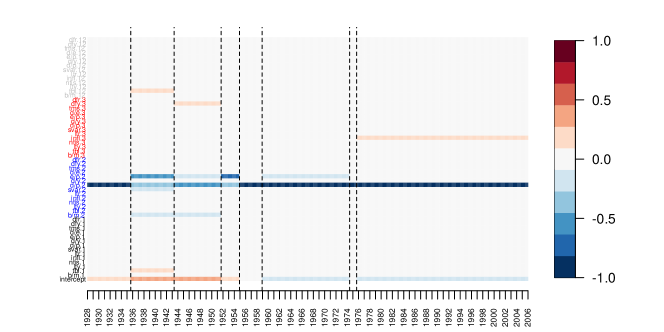
Figure 2: Equity premium data: Parameter estimates from each estimated segment obtained by MOSEG.MS. Variables at different lags are coloured differently in the $y$-axis.

We apply MOSEG.MS with $\mathcal{G}=\{72,96,120\}$ in line with the choice described in Section 4.1 but we select $G_{h}$ to be multiples of $12$ for interpretability as the observation frequency is monthly. MOSEG.MS returns $\widehat{q}=7$ change point estimators reported in Table 6, and takes $45$ seconds in total (including CV). When applied to the same dataset, DPDU takes $25$ minutes and VPWBS takes $15$ minutes, and neither detects any change point. In Figure 2, we plot the local parameter estimates obtained from each of the seven estimated segments. We can relate the change detected in $1954$ to the findings reported in Rapach et al., (2010), where they attribute the instability in the pairwise relationships between the equity premium and each of the $14$ variables to the Treasury-Federal Reserve Accord and the transition from the wartime economy. Dividend price ratio (d/p, at lag two) is active throughout the observation period which agrees with the observations made in Welch and Goyal, (2008). They also remark that the recession from $1973$ to $1975$ due to the Oil Shock drives the good predictive performance of many models proposed for equity premium forecasting, and most perform poorly over the $30$ year period ($1975$–$2005$) following the Oil Shock. The two last segments defined by the change point estimators reported in Table 6 are closely located with these important periods, which supports the validity of the segmentation returned by MOSEG.MS. We note that regardless of the choice of bandwidths, both of the two estimators in $1974$ and $1975$ defining the two periods are detected separately.

Table 6: Equity premium data: Change point estimators detected by MOSEG.MS.

Estimator	$\widehat{\theta}_{1}$	$\widehat{\theta}_{2}$	$\widehat{\theta}_{3}$	$\widehat{\theta}_{4}$	$\widehat{\theta}_{5}$	$\widehat{\theta}_{6}$	$\widehat{\theta}_{7}$
Date	Oct 1935	Apr 1943	Aug 1951	Nov 1954	Nov 1958	May 1974	Aug 1975

6 Conclusions

In this paper, we propose MOSEG, a high-dimensional data segmentation methodology for detecting multiple changes in the parameters under a linear regression model. It proceeds in two steps, first grid-based scanning of the data for large changes in local parameter estimators over a moving window, followed by a computationally efficient location refinement step. We further propose its multiscale extension, MOSEG.MS, which alleviates the necessity to select a single bandwidth. Both numerically and theoretically, we demonstrate the efficiency of the proposed methodologies. Computationally, they are highly competitive thanks to the careful design of the algorithms that limit the required number of Lasso estimators. Theoretically, we show the consistency of MOSEG and MOSEG.MS in a general setting permitting serial dependence and heavy tails and establish their (near-)minimax optimality under Gaussianity. In particular, the consistency of MOSEG.MS is derived for a parameter space that simultaneously permits large changes over short intervals and small changes over long stretches of stationarity, which is much broader than that typically adopted in the literature. Comparative simulation studies and findings from the application of MOSEG.MS to equity premium data support its efficacy. The R software implementing MOSEG and MOSEG.MS is available from https://github.com/Dom-Owens-UoB/moseg.

Appendix A Literature review and comparison with the existing methods

A.1 Under (sub-)Gaussianity

Table A.1 provides an overview of the theoretical properties of MOSEG and MOSEG.MS in comparison with the methods proposed in Wang et al., (2021), Kaul et al., 2019a and Xu et al., (2022) for the change point problem in (5) under Gaussianity, as well as their computational complexity.

Specifically, Table A.1 reports the separation and localisation rates associated with each method, which are defined as below. For a given methodology, let $\widehat{\mathcal{K}}$ denote the set of estimated change points. Then, when the magnitude of change $\Delta$, measured by either

$$\Delta^{(1)}=\min_{1\leq j\leq q}\delta_{j}^{2}\cdot\min_{0\leq j\leq q}(\theta_{j+1}-\theta_{j})\text{ \ or \ }\Delta^{(2)}=\min_{1\leq j\leq q}\delta_{j}^{2}\min(\theta_{j}-\theta_{j-1},\theta_{j+1}-\theta_{j}),$$

diverges faster than the separation rate $s_{n,p}$ associated with the method, all $q$ changes are detected by $\widehat{\mathcal{K}}$ with asymptotic power one and their locations are consistently estimated with the localisation rate $\ell_{n,p}$, such that $\min_{1\leq j\leq q}\min_{\widehat{k}\in\widehat{\mathcal{K}}}w_{j}|\widehat{k}-\theta_{j}|=O_{P}(\ell_{n,p})$. Here, $w_{j}$ refers to the relative difficulty in locating $\theta_{j}$ which is related to the jump size $\delta_{j}$.

Table A.1: Comparison of data segmentation methods developed for the model (5) in their theoretical properties under Gaussianity and computational complexity (for given tuning parameters). Here, $\mathfrak{s}=\max_{0\leq j\leq q}|\mathcal{S}_{j}|$ and $\mathfrak{S}=|\cup_{j=0}^{q}\mathcal{S}_{j}|$. Refer to the text for the definitions of $s_{n,p}$, $\ell_{n,p}$, $\Delta$ and $w_{j}$. For Xu et al., (2022), we report the rates associated with their preliminary estimators; see the text for further explanation.

	Separation		Localisation		Computational
	$s_{n,p}$	$\Delta$	$\ell_{n,p}$	$w_{j}$	complexity
MOSEG	$\mathfrak{s}\log(p\vee n)$	$\Delta^{(1)}$	$\mathfrak{s}\log(p\vee n)$	$\delta_{j}$	$O(\frac{n}{rG}\cdot\text{Lasso}(p))$
MOSEG.MS	$\mathfrak{s}\log(p\vee n)$	$\Delta^{(2)}$	$\mathfrak{s}\log(p\vee n)$	$\delta_{j}$	$O(\frac{n}{rG_{1}}\cdot\text{Lasso}(p))$
Wang et al., (2021)	$\mathfrak{s}\log(p\vee n)$	$\Delta^{(1)}$	$\mathfrak{s}\log(n)$	$\delta_{j}$	$O(n\log^{2}(n)\cdot\text{GroupLasso}(p))$
Kaul et al., 2019a	$\mathfrak{S}\log(p\vee n)$	$\Delta^{(1)}$	$\mathfrak{S}\log(p)$	$\delta$	$O(\tilde{q}\cdot\text{Lasso}(p)+\text{SA}(\tilde{q}))$
Xu et al., (2022)	$\mathfrak{s}\log(p\vee n)$	$\Delta^{(1)}$	$\mathfrak{s}\log(p\vee n)$	$\delta_{j}$	$O(n^{2}p^{2}+n^{2}\cdot\text{Lasso}(p))$

Wang et al., (2021) propose a method which learns the projection that is well-suited to reveal a change over each local segment and combines it with the wild binary segmentation algorithm (Fryzlewicz,, 2014) for multiple change point detection. Kaul et al., 2019a propose to minimise an $\ell_{0}$-penalised cost function given a set of candidate estimators of size $\tilde{q}$. Their theoretical analysis implicitly assumes that $\min_{j}(\theta_{j+1}-\theta_{j})$ scales linearly in $n$, and the simulated annealing adopted for minimising the penalised cost, denoted by SA($\tilde{q}$) in Table A.1, has complexity ranging from $O(\tilde{q}^{4})$ on average to being exponential in the worst case. In specifying the properties of Kaul et al., 2019a , the global sparsity $\mathfrak{S}=|\cup_{j=0}^{q}\mathcal{S}_{j}|$ can be much greater than the segment-wise sparsity $\mathfrak{s}$, particularly when the number of change points $q$ is large.

Xu et al., (2022) investigate the dynamic programming algorithm of Rinaldo et al., (2021) for minimising an $\ell_{0}$-penalised cost function in a general setting permitting non-Gaussianity and temporal dependence, as is the case in the current paper. In Table A.1, we report the separation and localisation rates derived in Xu et al., (2022) for their preliminary estimators from the dynamic programming algorithm. These estimators are further refined by a procedure similar to Stage 2 of MOSEG, which are shown to attain the rate $O_{P}(\delta_{j}^{-2})$ under a stronger condition on the size of changes, namely that $\Delta^{(1)}/(\mathfrak{s}^{2}\log^{3}(pn))\to\infty$. We note that the refined rate is derived for the individual change points, rather than when the estimation of multiple change points is simultaneously considered as is the case for the rates reported in Table A.1.

We also mention Zhang et al., (2015) where the data segmentation problem is treated as a high-dimensional regression problem with a group Lasso penalty, which only provides that the estimation bias is of $o_{P}(n)$. Leonardi and Bühlmann, (2016) consider both dynamic programming and binary segmentation algorithms are considered for change point estimation, and we refer to Rinaldo et al., (2021) for a detailed discussion on their results.

From Table A.1, we conclude that MOSEG.MS is highly competitive both computationally and statistically. We investigate the theoretical properties of MOSEG.MS in the broadest parameter space possible which is formulated with $\Delta^{(2)}$ instead of $\Delta^{(1)}$ as in all the other papers; recall that from the discussion following (21), we always have $\Delta^{(1)}\leq\Delta^{(2)}$ and the former can be much smaller than the latter when large shifts over short intervals and small changes over long stretches of stationarity are simultaneously present in the signal.

A.2 Beyond (sub-)Gaussianity and independence

The theoretical properties of MOSEG.MS reported in Table A.1 do not require independence or Gaussianity, unlike other works with the exception of Xu et al., (2022). In the presence of serial dependence and sub-Weibull tails (through having $\gamma>1$ as in Condition 1 (a)), Xu et al., (2022) require that $\Delta^{(1)}\gtrsim(\mathfrak{s}\log(np))^{4\gamma+2\gamma^{\prime}-1}$ for the detection of all change points, where a smaller value of $\gamma^{\prime}\in(0,\infty)$ imposes a faster decay of the serial dependence. This is comparable to the detection boundary of MOSEG, $\Delta^{(1)}\gtrsim(\mathfrak{s}\log(np))^{4\gamma+3}$, see Proposition 2 (i) and Corollary 3 (i). In characterising temporal dependence, Condition 1 considers linear processes with algebraically decaying dependence whereas $\gamma^{\prime}$ of Xu et al., (2022) governs the rate of exponentially decaying, possibly non-linear dependence. The localisation rate in Corollary 3 (i) is also comparable to that attained by the preliminary estimators of Xu et al., (2022) produced by a dynamic programming algorithm; as noted above, under a stronger condition on $\Delta^{(1)}$, they derive a further refined rate.

Appendix B Additional simulations

B.1 Choice of the grid

We investigate the performance of MOSEG as the coarseness of the grid varies with $r\in\{1/3,1/5,1/10,1/G\}$. Recall that when $r=1/G$, we use the full grid $\mathcal{T}=\{G,\ldots,n-G\}$ in Stage 1 of MOSEG, see (9). For this, we set $n=300$, $p=100$, $\mathfrak{s}=2$ and $q=1$, and generate the data under (5) with $\mathbf{x}_{t}\sim_{\text{iid}}\mathcal{N}_{p}(\mathbf{0},\mathbf{I})$ and $\varepsilon_{t}\sim_{\text{iid}}\mathcal{N}(0,1)$. For each realisation, the change point $\theta_{1}$ is randomly sampled from $\{51,\dots,250\}$. Varying $\delta\in\{0.1,0.2,0.4,0.8\}$, we generate $\bm{\beta}_{0}=(\beta_{0,1},\ldots,\beta_{0,p})^{\top}$ with $\beta_{0,i}=\delta\cdot(-1)^{i-1}$ for $i\in\{1,\ldots,\mathfrak{s}\}$ and have $\bm{\beta}_{1}=-\bm{\beta}_{0}$. Setting $G=50$, we select the maximiser of the MOSUM statistic as the pre-estimator $\widetilde{\theta}_{1}$ in Stage 1 of MOSEG, which then is refined as in (13) in Stage 2. Table B.1 reports the average and the standard error of $n^{-1}|\widetilde{\theta}_{1}-\theta_{1}|$ and $n^{-1}|\widehat{\theta}_{1}-\theta_{1}|$ over $100$ realisations when different grids are used. See also Figure B.1 which plots the Hausdorff distance $d_{H}$ (see (23)) against $r$. When the size of change is very small, estimators from both Stages 1 and 2 perform equally poorly regardless of the choice of $r$. However, as $\delta$ increases, we quickly observe that the estimation error becomes close to zero for the estimators from both stages provided that $r$ is not too large. Also, for $\delta\geq 0.2$, we observe that Stage 2 brings in small improvement in the localisation performance. From this, we conclude that the performance of MOSEG is robust to the choice of $r$ provided that it is chosen reasonably small, say $r\leq 1/5$.

Table B.1: Comparison of Hausdorff distance $d_{H}$ for Stage 1 and Stage 2 estimators from MOSEG when different grids are used. The average and the standard error of estimation errors over $100$ realisations are reported.

	$r=G^{-1}$				$r=1/10$
	Stage 1		Stage 2		Stage 1		Stage 2
$\delta$	Mean	SD	Mean	SD	Mean	SD	Mean	SD
0.1	0.2043	0.1561	0.2099	0.1670	0.2003	0.1525	0.2096	0.1683
0.2	0.1194	0.1367	0.1149	0.1442	0.1302	0.1402	0.1296	0.1549
0.4	0.0089	0.0104	0.0038	0.0053	0.0115	0.0179	0.0039	0.0050
0.8	0.0070	0.0089	0.0022	0.0052	0.0086	0.0096	0.0020	0.0049
	$r=1/5$				$r=1/3$
	Stage 1		Stage 2		Stage 1		Stage 2
$\delta$	Mean	SD	Mean	SD	Mean	SD	Mean	SD
0.1	0.2142	0.1525	0.2232	0.1683	0.2179	0.1525	0.2255	0.1683
0.2	0.1383	0.1402	0.1349	0.1549	0.2165	0.1402	0.2061	0.1549
0.4	0.0142	0.0179	0.0039	0.0050	0.2696	0.0179	0.2359	0.0050
0.8	0.0126	0.0096	0.0016	0.0049	0.2303	0.0096	0.1929	0.0049

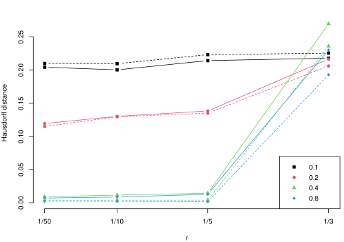
Figure B.1: Hausdorff distance $d_{H}$ against $r$ for Stage 1 (solid line) and Stage 2 (dashed line) estimators from MOSEG, as the size of changes varies.

B.2 Heavy-tailedness and temporal dependence

We examine the performance of MOSEG.MS, VPWBS (Wang et al.,, 2021) and DPDU (Xu et al.,, 2022) in the presence of heavy-tailed noise and temporal dependence. For this, we generate datasets with $n=300$, $p=100$, $\mathfrak{s}=10$ and $q=2$ where the two change points are located at $\theta_{j}=jn/3$, $j=1,2$. We use $\bm{\beta}_{0}$ generated as in Appendix B.1 with $\delta\in\{0.2,0.4,0.8,1.6\}$ and set $\bm{\beta}_{j}=(-1)^{j}\cdot\bm{\beta}_{0}$.

We consider the following three settings for the generation of $\mathbf{x}_{t}$ and $\varepsilon_{t}$.

1. $\mathbf{x}_{t}\sim_{\text{iid}}\mathcal{N}_{p}(\mathbf{0},\mathbf{I})$ and $\varepsilon_{t}\sim_{\text{iid}}\mathcal{N}(0,1)$ for all $t$.

2. $X_{it}\sim_{\text{iid}}\sqrt{3/5}\cdot t_{5}$ for all $i$ and $t$ and $\varepsilon_{t}\sim_{\text{iid}}\sqrt{3/5}\cdot t_{5}$ for all $t$.

3. $\{(\mathbf{x}_{t},\varepsilon_{t})\}_{t=1}^{n}$ is generated as in (16) where $\mathbf{D}_{1}$ is a diagonal matrix with $0.3$ on its diagonals, $\mathbf{D}_{\ell}=\mathbf{O}$ for $\ell\geq 2$ and $\bm{\zeta}_{t}\sim_{\text{iid}}\mathcal{N}_{p+1}(\mathbf{0},\sqrt{1-0.3^{2}}\mathbf{I})$ for all $t$.

Under (E2)–(E3), the data are permitted to be heavy-tailed and serially correlated, respectively; (E1) serves as a benchmark. Table B.2 reports the average and standard error of the Hausdorff distance in (23) and $\widehat{q}-q$ over $100$ realisations. It shows that generally, the performance of all three methods is less sensitive to heavy-tailedness or temporal dependence, compared to their sensitivity to the size of changes. VPWBS shows good localisation performance, while MOSEG.MS tends to achieve better detection accuracy when the size of change is small. DPDU performs very well in the more challenging setting with small $\delta$. However, as noted in Section 4, it is more prone to over-estimate the number of change points as $\delta$ increases with which the localisation performance also deteriorates.

Table B.2: Performance of MOSEG.MS and VPWBS under (E1)–(E3) over $100$ realisations. The best performer in each setting is denoted in bold.

			$\widehat{q}-q$
$\delta$	Setting	Method	$-2$	$-1$	0	1	2	$\geq$ 3	$d_{H}$
0.2	(E1)	MOSEG.MS	10	35	46	9	0	0	0.2905
		VPWBS	56	10	9	14	9	2	0.2583
		DPDU	0	0	86	12	1	1	0.0239
	(E2)	MOSEG.MS	6	53	34	6	1	0	0.2779
		VPWBS	60	10	7	13	10	0	0.2663
		DPDU	0	0	89	11	0	0	0.0168
	(E3)	MOSEG.MS	8	30	44	17	1	0	0.2644
		VPWBS	10	15	18	13	28	16	0.1671
		DPDU	0	0	85	13	2	0	0.0211
0.4	(E1)	MOSEG.MS	0	9	86	4	1	0	0.0766
		VPWBS	1	3	87	7	2	0	0.0361
		DPDU	0	0	82	16	1	1	0.0240
	(E2)	MOSEG.MS	1	11	83	5	0	0	0.0830
		VPWBS	1	7	83	4	5	0	0.0567
		DPDU	0	0	82	16	2	0	0.0248
	(E3)	MOSEG.MS	1	9	81	9	0	0	0.0678
		VPWBS	0	1	80	14	4	1	0.0397
		DPDU	0	0	71	24	5	0	0.0359
0.8	(E1)	MOSEG.MS	0	0	99	1	0	0	0.0119
		VPWBS	0	0	97	3	0	0	0.0095
		DPDU	0	0	81	18	1	0	0.0227
	(E2)	MOSEG.MS	0	0	98	2	0	0	0.0100
		VPWBS	0	0	98	2	0	0	0.0104
		DPDU	0	0	80	17	1	2	0.0209
	(E3)	MOSEG.MS	0	1	96	3	0	0	0.0153
		VPWBS	0	0	98	2	0	0	0.0103
		DPDU	0	0	73	24	3	0	0.0285
1.6	(E1)	MOSEG.MS	0	0	97	3	0	0	0.0097
		VPWBS	0	0	100	0	0	0	0.0037
		DPDU	0	0	75	22	1	2	0.0309
	(E2)	MOSEG.MS	0	0	100	0	0	0	0.0036
		VPWBS	0	0	100	0	0	0	0.0033
		DPDU	0	0	78	18	1	3	0.0249
	(E3)	MOSEG.MS	0	1	96	3	0	0	0.0076
		VPWBS	0	0	99	1	0	0	0.0045
		DPDU	0	0	69	24	6	1	0.0307

B.3 When the dimensionality is large

We additionally examine the case where $p=1000$, adopting the simulation setting (E1) from Appendix B.2. We exclude VPWBS (Wang et al.,, 2021) and DPDU (Xu et al.,, 2022) which, as shown in Section 4.2, tends to take considerably longer time to run compared to MOSEG.MS. Table B.3 shows that, in comparison to the the results under (E1) in Table B.2 obtained when $p=100$, the greater sample size is required to detect smaller changes. Also, the localisation performance worsens as $p$ increases. Nonetheless, MOSEG.MS demonstrates itself to be scalable as the dimensionality increases when the size of change is sufficiently large, which is in line with the theoretical requirements.

Table B.3: Performance of MOSEG.MS under (E1) when $\mathbf{p=1000}$ over $100$ realisations.

	$\widehat{q}-q$
$\delta$	$-2$	$-1$	0	1	2	$\geq$ 3	$d_{H}$
0.2	6	47	29	18	0	0	0.3051
0.4	10	34	44	11	1	0	0.2972
0.8	1	22	65	11	1	0	0.1391
1.6	4	3	92	1	0	0	0.0673

Appendix C Proofs

In what follows, for any vector $\mathbf{a}\in\mathbb{R}^{p}$ and a set $\mathcal{A}\subset\{1,\ldots,p\}$, we denote by $\mathbf{a}(\mathcal{A})=(a_{i},\,i\in\mathcal{A})^{\top}$ the sub-vector of $\mathbf{a}$ supported on $\mathcal{A}$. We write the population counterpart of $T_{k}(G)$ with $\bm{\beta}_{s,e}^{*}$ defined in (8) as

$$T^{*}_{k}(G)=\sqrt{\frac{G}{2}}\left|\bm{\beta}^{*}_{k,k+G}-\bm{\beta}^{*}_{k-G,k}\right|_{2}.$$

Further, we write $\mathcal{S}_{s,e}=\text{supp}(\bm{\beta}^{*}_{s,e})$.

C.1 Proof of Theorem 1

C.1.1 Supporting lemmas

Lemma C.1.

We have

$$T^{*}_{k}(G)=\left\{\begin{array}[]{ll}\frac{1}{\sqrt{2G}}(G-|k-\theta_{j}|)\delta_{j}&\text{if }\{k-G+1,\ldots,k+G\}\cap\Theta=\{\theta_{j}\},\\ 0&\text{if }\{k-G+1,\ldots,k+G\}\cap\Theta=\emptyset\\ \end{array}\right.$$

Lemma C.2.

Define $\bm{\Delta}_{s,e}=\widehat{\bm{\beta}}_{s,e}-\bm{\beta}^{*}_{s,e}$. With $\lambda\geq 4C_{\text{\tiny dev}}\rho_{n,p}$, we have $\mathsf{P}(\mathcal{B})\geq 1-\mathsf{P}(\mathcal{R}^{(1)}\cap\mathcal{D}^{(2)})$ where

$$\mathcal{B} =\left\{\left|\bm{\Delta}_{s,e}\right|_{2}\leq\frac{12\sqrt{2\mathfrak{s}}\lambda}{\omega\sqrt{e-s}}\text{ and }\left|\bm{\Delta}_{s,e}(\mathcal{S}_{s,e}^{c})\right|_{1}\leq 3\left|\bm{\Delta}_{s,e}(\mathcal{S}_{s,e})\right|_{1}\text{ for all }0\leq s<e\leq n\right.$$

$$\left.\text{ with }|\{s+1,\ldots,e\}\cap\Theta|\leq 1\text{ and }e-s\geq C_{0}\max\left[(\omega^{-1}\mathfrak{s}\log(p))^{\frac{1}{1-\tau}},\rho^{2}_{n,p}\right]\right\}.$$

Proof.

For given $0\leq s<e\leq n$, we have

$$\sum_{t=s+1}^{e}\left(Y_{t}-\mathbf{x}_{t}^{\top}\widehat{\bm{\beta}}_{s,e}\right)^{2}+\lambda\sqrt{e-s}|\widehat{\bm{\beta}}_{s,e}|_{1}\leq\sum_{t=s+1}^{e}\left(Y_{t}-\mathbf{x}_{t}^{\top}\bm{\beta}^{*}_{s,e}\right)^{2}+\lambda\sqrt{e-s}|\bm{\beta}^{*}_{s,e}|_{1},$$

from which it follows that

$$\lambda\sqrt{e-s}\left(|\bm{\beta}^{*}_{s,e}|_{1}-|\widehat{\bm{\beta}}_{s,e}|_{1}\right) \geq\sum_{t=s+1}^{e}\left[(\mathbf{x}_{t}^{\top}\widehat{\bm{\beta}}_{s,e})^{2}-(\mathbf{x}_{t}^{\top}\bm{\beta}^{*}_{s,e})^{2}-2Y_{t}\mathbf{x}_{t}^{\top}(\widehat{\bm{\beta}}_{s,e}-\bm{\beta}^{*}_{s,e})\right]$$

$$=\sum_{t=s+1}^{e}\left[\bm{\Delta}_{s,e}^{\top}\mathbf{x}_{t}\mathbf{x}_{t}^{\top}\bm{\Delta}_{s,e}-2(Y_{t}-\mathbf{x}_{t}^{\top}\bm{\beta}^{*}_{s,e})\mathbf{x}_{t}^{\top}\bm{\Delta}_{s,e}\right].$$

Then, noting that $\bm{\beta}^{*}_{s,e}(\mathcal{S}_{s,e}^{c})=\mathbf{0}$,

$$\frac{1}{\sqrt{e-s}}\sum_{t=s+1}^{e}\left[\bm{\Delta}_{s,e}^{\top}\mathbf{x}_{t}\mathbf{x}_{t}^{\top}\bm{\Delta}_{s,e}-2(Y_{t}-\mathbf{x}_{t}^{\top}\bm{\beta}^{*}_{s,e})\mathbf{x}_{t}^{\top}\bm{\Delta}_{s,e}\right]+\lambda\left|\widehat{\bm{\beta}}_{s,e}(\mathcal{S}_{s,e}^{c})\right|_{1}$$

$$\leq\lambda\left(\left|\bm{\beta}^{*}_{s,e}(\mathcal{S}_{s,e})\right|_{1}-\left|\widehat{\bm{\beta}}_{s,e}(\mathcal{S}_{s,e})\right|_{1}\right)\leq\lambda\left|\bm{\Delta}_{s,e}(\mathcal{S}_{s,e})\right|_{1}.$$ (C.1)

Since $\lambda\geq 4C_{\text{\tiny dev}}\rho_{n,p}$, it follows from (C.1) that on $\mathcal{D}^{(2)}$,

$$\frac{1}{\sqrt{e-s}}\sum_{t=s+1}^{e}\bm{\Delta}_{s,e}^{\top}\mathbf{x}_{t}\mathbf{x}_{t}^{\top}\bm{\Delta}_{s,e}-\frac{\lambda}{2}\left|\bm{\Delta}_{s,e}\right|_{1}+\lambda\left|\bm{\Delta}_{s,e}(\mathcal{S}_{s,e}^{c})\right|_{1}\leq\lambda\left|\bm{\Delta}_{s,e}(\mathcal{S}_{s,e})\right|_{1},$$

$$\therefore\,0\leq\frac{1}{\sqrt{e-s}}\sum_{t=s+1}^{e}\bm{\Delta}_{s,e}^{\top}\mathbf{x}_{t}\mathbf{x}_{t}^{\top}\bm{\Delta}_{s,e}\leq\frac{\lambda}{2}\left(3\left|\bm{\Delta}_{s,e}(\mathcal{S}_{s,e})\right|_{1}-\left|\bm{\Delta}_{s,e}(\mathcal{S}_{s,e}^{c})\right|_{1}\right),$$

such that

$$\left|\bm{\Delta}_{s,e}(\mathcal{S}_{s,e}^{c})\right|_{1}\leq 3\left|\bm{\Delta}_{s,e}(\mathcal{S}_{s,e})\right|_{1}.$$ (C.2)

This in particular leads to

$$\left|\bm{\Delta}_{s,e}\right|_{1}\leq 4\left|\bm{\Delta}_{s,e}(\mathcal{S}_{s,e})\right|_{1}\leq 4\sqrt{2\mathfrak{s}}\left|\bm{\Delta}_{s,e}\right|_{2}$$

from the definition of $\mathfrak{s}$. Then on $\mathcal{R}^{(1)}$, we have

$$6\sqrt{2\mathfrak{s}}\lambda\left|\bm{\Delta}_{s,e}\right|_{2} \geq\frac{1}{\sqrt{e-s}}\sum_{t=s+1}^{e}\bm{\Delta}_{s,e}^{\top}\mathbf{x}_{t}\mathbf{x}_{t}^{\top}\bm{\Delta}_{s,e}$$

$$\geq\omega\sqrt{e-s}\left|\bm{\Delta}_{s,e}\right|_{2}^{2}-\frac{32C_{\text{\tiny RE}}\mathfrak{s}\log(p)(e-s)^{\tau}}{\sqrt{e-s}}\left|\bm{\Delta}_{s,e}\right|_{2}^{2}\geq\frac{\omega}{2}\sqrt{e-s}\left|\bm{\Delta}_{s,e}\right|_{2}^{2},$$

where the last inequality follows for $(e-s)^{1-\tau}\geq 64C_{\text{\tiny RE}}\omega^{-1}\mathfrak{s}\log(p)$. In summary,

$$\left|\bm{\Delta}_{s,e}\right|_{2}\leq\frac{12\sqrt{2\mathfrak{s}}\lambda}{\omega\sqrt{e-s}}.$$ (C.3)

Combining (C.2) and (C.3), the proof is complete. ∎

C.1.2 Proof of Theorem 1 (i)

Let $\mathcal{T}_{j}=\{\theta_{j}-\lfloor\eta G\rfloor+1,\ldots,\theta_{j}+\lfloor\eta G\rfloor\}\cap\mathcal{T}$ for $1\leq j\leq q$. Under Assumptions 4 and 5, we have $G\geq C_{\delta}^{-2}C_{1}\max\{\omega^{-2}\mathfrak{s}\rho_{n,p}^{2},(\omega^{-1}\mathfrak{s}\log(p))^{1/(1-\tau)}\}$ such that the lower bound on $(e-s)$ made in $\mathcal{B}$ (see Lemma C.2) is met by all $s=k$ and $e=k+G$, $k=0,\ldots,n-G$. By Lemma C.2,

$$\max_{G\leq k\leq n-G}\left|T_{k}(G)-T^{*}_{k}(G)\right|\leq$$

$$\max_{G\leq k\leq n-G}\sqrt{\frac{G}{2}}\left(\left|\widehat{\bm{\beta}}_{k-G,k}-\bm{\beta}^{*}_{k-G,k}\right|_{2}+\left|\widehat{\bm{\beta}}_{k,k+G}-\bm{\beta}^{*}_{k,k+G}\right|_{2}\right)\leq\frac{24\sqrt{\mathfrak{s}}\lambda}{\omega}.$$ (C.4)

First, consider some $k$ for which $\{k-G+2,\ldots,k+G-1\}\cap\Theta=\emptyset$. Then, we have $T^{*}_{k}(G)=0$ from Lemma C.1 such that by (C.4),

$$\max_{k:\,\min_{1\leq j\leq q}|k-\theta_{j}|\geq G}T_{k}(G)\leq\max_{G\leq\ell\leq n-G}\left|T_{\ell}(G)-T^{*}_{\ell}(G)\right|\leq\frac{24\sqrt{\mathfrak{s}}\lambda}{\omega}\leq D.$$ (C.5)

This ensures that any $\widetilde{\theta}\in\widetilde{\Theta}$ satisfies $\min_{1\leq j\leq q}|\widetilde{\theta}-\theta_{j}|<G$. Next, let $\theta^{\text{\tiny L}}_{j}$ and $\theta^{\text{\tiny R}}_{j}$ denote two points within $\mathcal{T}_{j}$ which are the closest to $\theta_{j}$ from the left and and the right of $\theta_{j}$, respectively, with $\theta^{\text{\tiny L}}_{j}=\theta^{\text{\tiny R}}_{j}$ when $r=1/G$. Then by construction of $\mathcal{T}$,

$$\max(k_{j}-\theta^{\text{\tiny L}}_{j},\theta^{\text{\tiny R}}_{j}-\theta_{j})\leq\lfloor rG\rfloor\quad\text{and}\quad\min(\theta_{j}-\theta^{\text{\tiny L}}_{j},\theta^{\text{\tiny R}}_{j}-\theta_{j})\leq\frac{\lfloor rG\rfloor}{2},$$ (C.6)

such that from Lemma C.1,

$$\max\left(T^{*}_{\theta^{\text{\tiny L}}_{j}}(G),T^{*}_{\theta^{\text{\tiny R}}_{j}}(G)\right)\geq\frac{\delta_{j}(G-\lfloor rG\rfloor/2)}{\sqrt{2G}}\geq\sqrt{\frac{G}{2}}\delta_{j}(1-r/2).$$

From this and by (C.4), at $\widetilde{\theta}_{j}=\arg\max_{k\in\mathcal{T}_{j}}T_{k}(G)$, we have

$$T_{\widetilde{\theta}_{j}}(G)\geq\max\left(T_{\theta^{\text{\tiny L}}_{j}}(G),T_{\theta^{\text{\tiny R}}_{j}}(G)\right)\geq\sqrt{\frac{G}{2}}\delta_{j}\left(1-\frac{r}{2}\right)-\frac{24\sqrt{\mathfrak{s}}\lambda}{\omega}>\frac{1-r/2}{2}\sqrt{\frac{G}{2}}\delta_{j}>D,$$

where the second last inequality follows from Assumption 5 (b), and the last one from (15). When $\eta=1$, this and (C.5) indicates that such $\widetilde{\theta}_{j}$ satisfies (10). When $\eta<1$, note that

$$\max\left(T_{\theta^{\text{\tiny L}}_{j}}(G),T_{\theta^{\text{\tiny R}}_{j}}(G)\right)-\max\left\{T_{k}(G):\,|k-\theta_{j}|>(1-\eta)G,\,k\in\mathcal{T}\right\}$$

$$\geq\sqrt{\frac{G}{2}}\delta_{j}\left(\eta-\frac{3r}{2}\right)-\frac{48\sqrt{\mathfrak{s}}\lambda}{\omega}\geq\frac{5\eta}{8\sqrt{2}}\min_{1\leq j\leq q}\delta_{j}\sqrt{G}-\frac{48\sqrt{\mathfrak{s}}\lambda}{\omega}>0$$

from (15). These arguments ensure that we detect at least one change point in $\mathcal{T}_{j}$ at $t=\widetilde{\theta}_{j}$ for each $j=1,\ldots,q$. For such $\widetilde{\theta}_{j}$, suppose that $\theta^{\circ}_{j}={\arg\min}_{k\in\{\theta^{\text{\tiny L}}_{j},\theta^{\text{\tiny R}}_{j}\}}|\widetilde{\theta}_{j}-k|$. Then,

$$\frac{\delta_{j}}{\sqrt{2G}}(G-|\widetilde{\theta}_{j}-\theta_{j}|)+\frac{24\sqrt{\mathfrak{s}}\lambda}{\omega}\geq T_{\widetilde{\theta}_{j}}(G)\geq T_{\theta^{\circ}_{j}}(G)\geq\frac{\delta_{j}}{\sqrt{2G}}(G-|\theta^{\circ}_{j}-\theta_{j}|)-\frac{24\sqrt{\mathfrak{s}}\lambda}{\omega}$$

and re-arranging, we obtain

$$\frac{\delta_{j}}{\sqrt{2G}}\left(|\widetilde{\theta}_{j}-\theta_{j}|-|\theta^{\circ}_{j}-\theta_{j}|\right)\leq\frac{48\sqrt{\mathfrak{s}}\lambda}{\omega},\text{ such that }|\widetilde{\theta}_{j}-\theta_{j}|\leq\frac{48\sqrt{2\mathfrak{s}G}\lambda}{\omega\delta_{j}}+\lfloor rG\rfloor<\left\lfloor\frac{G}{2}\right\rfloor,$$

for large enough $C_{1}$ in Assumption 5 (b).

Finally, let $\mathcal{L}_{\mathcal{T}}(t)$ denote the largest time point $k^{\prime}\in\mathcal{T}$ that satisfies $k^{\prime}\leq t$, and define $\mathcal{R}_{\mathcal{T}}(t)$ analogously. Then, we establish that

$$T_{\mathcal{L}_{\mathcal{T}}(\theta_{j}-\frac{\eta G}{2}m)}(G)>\max\left\{T_{k}(G):\,\frac{\eta G}{2}(m+1)\leq\theta_{j}-k\leq\frac{\eta G}{2}(m+2),\,k\in\mathcal{T}\right\},$$ (C.7)

$$T_{\mathcal{R}_{\mathcal{T}}(\theta_{j}+\frac{\eta G}{2}m)}(G)>\max\left\{T_{k}(G):\,\frac{\eta G}{2}(m+1)\leq k-\theta_{j}\leq\frac{\eta G}{2}(m+2),\,k\in\mathcal{T}\right\},$$ (C.8)

for $m=0,\ldots,\lceil 2/\eta\rceil-2$. The inequality in (C.7) follows from noting that

$$T_{\mathcal{L}_{\mathcal{T}}(\theta_{j}-\frac{\eta G}{2}m)}(G)-\max\left\{T_{k}(G):\,\frac{\eta G}{2}(m+1)\leq\theta_{j}-k\leq\frac{\eta G}{2}(m+2),\,k\in\mathcal{T}\right\}$$

$$\geq\sqrt{\frac{G}{2}}\delta_{j}\left(\frac{\eta}{2}-r\right)-\frac{48\sqrt{\mathfrak{s}}\lambda}{\omega}\geq\frac{\eta}{4\sqrt{2}}\min_{1\leq j\leq q}\delta_{j}\sqrt{G}-\frac{48\sqrt{\mathfrak{s}}\lambda}{\omega}>0$$

under (15), and the inequality in (C.8) follows analogously. This ensures that $\widetilde{\theta}_{j}$ by its construction is the unique local maximiser of $T_{k}(G)$ within the interval $\{\theta_{j}-G+1,\ldots,\theta_{j}+G\}\cap\mathcal{T}$ satisfying (10) for each $j=1,\ldots,q$, which completes the proof.

C.1.3 Proof of Theorem 1 (ii)

Recalling (11), we write

$$Q_{j}(k)=\sum_{t=\widetilde{\theta}_{j}-G+1}^{k}(Y_{t}-\mathbf{x}_{t}^{\top}\widehat{\bm{\beta}}^{\text{\tiny L}}_{j})^{2}+\sum_{t=k+1}^{\widetilde{\theta}_{j}+G}(Y_{t}-\mathbf{x}_{t}^{\top}\widehat{\bm{\beta}}^{\text{\tiny R}}_{j})^{2}.$$

Theorem 1 (i) establishes that for each $j=1,\ldots,q$, we have $\widetilde{\theta}_{j}\in\widetilde{\Theta}$ that satisfies $|\widetilde{\theta}_{j}-\theta_{j}|<G/2$, and $\widetilde{\Theta}$ contains no other estimator. Then under Assumption 5 (a), we have the following statements satisfied for all $j$.

1. Defining $\mathcal{I}(\widetilde{\theta}_{j})=\{\widetilde{\theta}_{j}-G+1,\ldots,\widetilde{\theta}_{j}+G\}$, it fulfils $\mathcal{I}(\widetilde{\theta}_{j})\cap\Theta=\{\theta_{j}\}$.

2. $\{\widetilde{\theta}^{\text{\tiny L}}_{j}-G+1,\ldots,\widetilde{\theta}^{\text{\tiny L}}_{j}\}\subset\{\theta_{j-1}+1,\ldots,\theta_{j}\}$ and $\{\widetilde{\theta}^{\text{\tiny R}}_{j}+1,\ldots,\widetilde{\theta}^{\text{\tiny R}}_{j}+G\}\subset\{\theta_{j}+1,\ldots,\theta_{j+1}\}$, such that denoting by $\bm{\Delta}^{\text{\tiny L}}_{j}=\widehat{\bm{\beta}}^{\text{\tiny L}}_{j}-\bm{\beta}_{j-1}$ and $\bm{\Delta}^{\text{\tiny R}}_{j}=\widehat{\bm{\beta}}^{\text{\tiny R}}_{j}-\bm{\beta}_{j}$, we have

   $$\max\left(\left|\bm{\Delta}^{\text{\tiny L}}_{j}\right|_{2},\left|\bm{\Delta}^{\text{\tiny R}}_{j}\right|_{2}\right)\leq\frac{12\sqrt{2\mathfrak{s}}\lambda}{\omega\sqrt{G}},$$

   $$\left|\bm{\Delta}^{\text{\tiny L}}_{j}(\mathcal{S}_{j-1}^{c})\right|_{1}\leq 3\left|\bm{\Delta}^{\text{\tiny L}}_{j}(\mathcal{S}_{j-1})\right|_{1}\text{ and }\left|\bm{\Delta}^{\text{\tiny R}}_{j}(\mathcal{S}_{j}^{c})\right|_{1}\leq 3\left|\bm{\Delta}^{\text{\tiny R}}_{j}(\mathcal{S}_{j})\right|_{1}$$ (C.9)

   in $\mathcal{B}$, see Lemma C.2.

Then we show that for all $k\in\mathcal{I}(\widetilde{\theta}_{j})$ satisfying $\delta_{j}^{2}|k-\theta_{j}|>v_{n,p}$ with

$$v_{n,p}=\max\left(\mathfrak{s}\rho_{n,p}^{2},\left(\mathfrak{s}\log(p)\right)^{\frac{1}{1-\tau}}\right)\cdot\max\left\{C_{\delta}^{2}\max\left[\frac{9C_{\text{\tiny RE}}}{2\omega},\frac{32C_{\text{\tiny RE}}}{\bar{\omega}}\right]^{\frac{1}{1-\tau}},\left(\frac{96C_{\text{\tiny dev}}}{\omega}\right)^{2}\right\},$$ (C.10)

we have $Q_{j}(k)-Q_{j}(\theta_{j})>0$, which completes the proof.

First, suppose that $k\geq\theta_{j}+1$. Then,

$$Q_{j}(k)-Q_{j}(\theta_{j})=\sum_{t=\theta_{j}+1}^{k}\left[(Y_{t}-\mathbf{x}^{\top}_{t}\widehat{\bm{\beta}}^{\text{\tiny L}}_{j})^{2}-(Y_{t}-\mathbf{x}^{\top}_{t}\widehat{\bm{\beta}}^{\text{\tiny R}}_{j})^{2}\right]$$

$$= \sum_{t=\theta_{j}+1}^{k}(\bm{\beta}_{j}-\widehat{\bm{\beta}}^{\text{\tiny L}}_{j})^{\top}\mathbf{x}_{t}\mathbf{x}_{t}^{\top}(\bm{\beta}_{j}-\widehat{\bm{\beta}}^{\text{\tiny L}}_{j})-\sum_{t=\theta_{j}+1}^{k}(\widehat{\bm{\beta}}^{\text{\tiny R}}_{j}-\bm{\beta}_{j})^{\top}\mathbf{x}_{t}\mathbf{x}_{t}^{\top}(\widehat{\bm{\beta}}^{\text{\tiny R}}_{j}-\bm{\beta}_{j})$$

$$+2\sum_{t=\theta_{j}+1}^{k}\varepsilon_{t}\mathbf{x}_{t}^{\top}\left[(\bm{\beta}_{j}-\bm{\beta}_{j-1})+(\widehat{\bm{\beta}}^{\text{\tiny R}}_{j}-\bm{\beta}_{j})-(\widehat{\bm{\beta}}^{\text{\tiny L}}_{j}-\bm{\beta}_{j-1})\right]=I_{1}+I_{2}+I_{3}.$$

From the definition of $\mathfrak{s}$ and the Cauchy-Schwarz inequality,

$$|\bm{\beta}_{j}-\bm{\beta}_{j-1}|_{1}\leq\sqrt{2\mathfrak{s}}|\bm{\beta}_{j}-\bm{\beta}_{j-1}|_{2}$$ (C.11)

and from (C.9), we have

$$|\bm{\Delta}^{\text{\tiny L}}_{j}|_{1}\leq 4|\bm{\Delta}^{\text{\tiny L}}_{j}(\mathcal{S}_{j})|_{1}\leq 4\sqrt{2\mathfrak{s}}|\bm{\Delta}^{\text{\tiny L}}_{j}|_{2}\text{ and analogously, }|\bm{\Delta}^{\text{\tiny R}}_{j}|_{1}\leq 4\sqrt{2\mathfrak{s}}|\bm{\Delta}^{\text{\tiny R}}_{j}|_{2}.$$ (C.12)

From (C.11)–(C.12), we derive

$$\left|\widehat{\bm{\beta}}^{\text{\tiny L}}_{j}-\bm{\beta}_{j}\right|_{2}\leq\delta_{j}\left(1+\frac{12\sqrt{2\mathfrak{s}}\lambda}{\omega\delta_{j}\sqrt{G}}\right)\leq\frac{3\delta_{j}}{2}\text{ and similarly, }\left|\widehat{\bm{\beta}}^{\text{\tiny L}}_{j}-\bm{\beta}_{j}\right|_{2}\geq\frac{\delta_{j}}{2},$$

$$\left|\widehat{\bm{\beta}}^{\text{\tiny L}}_{j}-\bm{\beta}_{j}\right|_{1}\leq\sqrt{\mathfrak{s}}\delta_{j}\left(1+\frac{96\sqrt{\mathfrak{s}}\lambda}{\omega\delta_{j}\sqrt{G}}\right)\leq\frac{3\sqrt{\mathfrak{s}}\delta_{j}}{2},$$

for a large enough $C_{1}$ in Assumption 5 (b). Then on $\mathcal{R}^{(1)}$, we have

$$I_{1}\geq|k-\theta_{j}|\omega\delta_{j}^{2}\left(\frac{1}{4}-\frac{9C_{\text{\tiny RE}}\mathfrak{s}\log(p)}{4|k-\theta_{j}|^{1-\tau}\omega}\right)\geq\frac{\omega}{8}\delta_{j}^{2}|k-\theta_{j}|$$ (C.13)

from that $|k-\theta_{j}|>\delta_{j}^{-2}v_{n,p}\geq C_{\delta}^{-2}v_{n,p}$ (from Assumption 4) and (C.10). As for $I_{2}$, from Lemma C.2, (C.10) and (C.12) we have on $\mathcal{R}^{(2)}$,

$$\left|I_{2}\right|\leq\left|\bm{\Delta}^{\text{\tiny R}}_{j}\right|_{2}^{2}\left[|k-\theta_{j}|\bar{\omega}+32C_{\text{\tiny RE}}\mathfrak{s}\log(p)|k-\theta_{j}|^{\tau}\right]\leq 2|k-\theta_{j}|\bar{\omega}\left|\bm{\Delta}^{\text{\tiny R}}_{j}\right|_{2}^{2}\leq\frac{576\bar{\omega}\mathfrak{s}|k-\theta_{j}|\lambda^{2}}{\omega^{2}G}.$$ (C.14)

Turning our attention to $I_{3}$, from (C.11)–(C.12),

$$\left|(\bm{\beta}_{j}-\bm{\beta}_{j-1})+(\widehat{\bm{\beta}}^{\text{\tiny R}}_{j}-\bm{\beta}_{j})-(\widehat{\bm{\beta}}^{\text{\tiny L}}_{j}-\bm{\beta}_{j-1})\right|_{1}\leq\left|\bm{\beta}_{j}-\bm{\beta}_{j-1}\right|_{1}+\left|\widehat{\bm{\beta}}^{\text{\tiny R}}_{j}-\bm{\beta}_{j}\right|_{1}+\left|\widehat{\bm{\beta}}^{\text{\tiny L}}_{j}-\bm{\beta}_{j-1}\right|_{1}$$

$$\leq\sqrt{\mathfrak{s}}\delta_{j}\left(1+\frac{192\sqrt{\mathfrak{s}}\lambda}{\omega\delta_{j}\sqrt{G}}\right)\leq 2\sqrt{\mathfrak{s}}\delta_{j},$$

where the last inequality follows from Assumption 5 (b). Then on $\mathcal{D}^{(1)}$,

$$\frac{1}{2}\left|I_{3}\right| \leq\left|\sum_{t=\theta_{j}+1}^{k}\varepsilon_{t}\mathbf{x}_{t}^{\top}\right|_{\infty}\;\left|(\bm{\beta}_{j}-\bm{\beta}_{j-1})+(\widehat{\bm{\beta}}^{\text{\tiny R}}_{j}-\bm{\beta}_{j})-(\widehat{\bm{\beta}}^{\text{\tiny L}}_{j}-\bm{\beta}_{j-1})\right|_{1}$$

$$\leq 2C_{\text{\tiny dev}}\delta_{j}\sqrt{\mathfrak{s}(k-\theta_{j})}\rho_{n,p}.$$ (C.15)

Then from (C.13), (C.14) and (C.15), we derive

$$\frac{|I_{2}|}{I_{1}}=\frac{4608\bar{\omega}\mathfrak{s}\lambda^{2}}{\omega^{3}\delta_{j}^{2}G}\leq\frac{1}{3}\quad\text{and}\quad\frac{|I_{3}|}{I_{1}}=\frac{32C_{\text{\tiny dev}}\sqrt{\mathfrak{s}}\rho_{n,p}}{\omega\delta_{j}\sqrt{k-\theta_{j}}}\leq\frac{1}{3}$$

under Assumption 5 (b), for all $k\in\mathcal{I}_{j}$ satisfying $\delta_{j}^{2}|k-\theta_{j}|>v_{n,p}$ from (C.10). Analogous arguments apply when $k\leq\theta_{j}$, and the above arguments are deterministic on $\mathcal{M}$. In summary, we have

$$\min_{1\leq j\leq q}\min_{\begin{subarray}{c}k\in\mathcal{I}_{j}\\ \delta_{j}^{2}|k-\theta_{j}|>v_{n,p}\end{subarray}}\left(Q_{j}(k)-Q_{j}(\theta_{j})\right)>\frac{\omega}{24}v_{n,p}>0,$$

which concludes the proof.

C.2 Proof of Proposition 2

C.2.1 Supporting lemmas

Define $\mathbb{K}(b)=\mathbb{B}_{0}(b)\cap\mathbb{B}_{2}(1)$ with some $b\geq 1$, where $\mathbb{B}_{d}(r)=\{\mathbf{a}:\,|\mathbf{a}|_{d}\leq r\}$ with the dimension of $\mathbf{a}$ determined within the context. Let $\mathbf{e}_{i}$ denote a vector that contains zeros except for its $i$th component set to be one. We denote the time-varying vector of parameters under (5) by $\bm{\beta}(t)=\sum_{j=1}^{q+1}\bm{\beta}_{j}\mathbb{I}_{\{\theta_{j-1}+1\leq t\leq\theta_{j}\}}$.

Denote by $\mathbf{Z}_{t}=(\mathbf{x}_{t}^{\top},\varepsilon_{t})^{\top}\in\mathbb{R}^{p+1}$ which admits $\mathbf{Z}_{t}=\sum_{\ell=0}^{\infty}\mathbf{D}_{\ell}\bm{\xi}_{t-\ell}$ under (16). For some $\mathbf{a},\mathbf{b}\in\mathbb{B}_{2}(1)$, define $U_{t}(\mathbf{a})=\mathbf{a}^{\top}\mathbf{Z}_{t}$ and $W_{t}(\mathbf{a},\mathbf{b})=\mathbf{a}^{\top}\mathbf{Z}_{t}\mathbf{Z}_{t}^{\top}\mathbf{b}$. Let $\bm{\xi}_{t}^{\prime}$ denote an independent copy of $\bm{\xi}_{t}$, and define $\mathbf{Z}_{t,\{0\}}=\sum_{\ell=0,\,\ell\neq t}^{\infty}\mathbf{D}_{\ell}\bm{\xi}_{t-\ell}+\mathbf{D}_{t}\bm{\xi}^{\prime}_{0}$. We denote the functional dependence measure and the dependence-adjusted norm for $U_{t}(\mathbf{a})$ as defined in Zhang and Wu, (2017), by

$$\delta_{t,\nu}(\mathbf{a})=\left\|\mathbf{a}^{\top}\mathbf{Z}_{t}-\mathbf{a}^{\top}\mathbf{Z}_{t,\{0\}}\right\|_{\nu}\quad\text{and}\quad{\left|\kern-1.07639pt\left|\kern-1.07639pt\left|U_{\cdot}(\mathbf{a})\right|\kern-1.07639pt\right|\kern-1.07639pt\right|}_{\nu}=\sum_{t=0}^{\infty}\delta_{t,\nu}(\mathbf{a}),$$

respectively. Analogously, we define

$$\delta_{t,\nu}(\mathbf{a},\mathbf{b})=\left\|\mathbf{a}^{\top}\mathbf{Z}_{t}\mathbf{Z}_{t}^{\top}\mathbf{b}-\mathbf{a}^{\top}\mathbf{Z}_{t,\{0\}}\mathbf{Z}_{t,\{0\}}^{\top}\mathbf{b}\right\|_{\nu}\quad\text{and}\quad{\left|\kern-1.07639pt\left|\kern-1.07639pt\left|W_{\cdot}(\mathbf{a},\mathbf{b})\right|\kern-1.07639pt\right|\kern-1.07639pt\right|}_{\nu}=\sum_{t=0}^{\infty}\delta_{t,\nu}(\mathbf{a},\mathbf{b})$$

for $W_{t}(\mathbf{a},\mathbf{b})$. Finally, for some $\kappa\geq 0$, we denote the dependence adjusted sub-exponential norm of $W_{t}(\mathbf{a},\mathbf{b})$ by $\|W_{\cdot}(\mathbf{a},\mathbf{b})\|_{\psi_{\kappa}}=\sup_{\nu\geq 2}\nu^{-\kappa}{\left|\kern-1.07639pt\left|\kern-1.07639pt\left|W_{\cdot}(\mathbf{a},\mathbf{b})\right|\kern-1.07639pt\right|\kern-1.07639pt\right|}_{\nu}$. In what follows, we denote by $C_{\Pi}$ with $\Pi\subset\{\gamma,\nu,\Xi,\varsigma\}$ a constant that depends on the parameters included in $\Pi$ which may vary from one occasion to another.

Lemma C.3.

Suppose that Condition 1 holds.

1. Under Condition 1 (a), we have $\sup_{\mathbf{a},\mathbf{b}\in\mathbb{B}_{2}(1)}\|W_{\cdot}(\mathbf{a},\mathbf{b})\|_{\psi_{\kappa}}\leq C_{\gamma,\Xi,\varsigma}C_{\xi}^{2}<\infty$ with $\kappa=2\gamma+1$.

2. Under Condition 1 (b), we have $\sup_{\mathbf{a}\in\mathbb{B}_{2}(1)}{\left|\kern-1.07639pt\left|\kern-1.07639pt\left|U_{\cdot}(\mathbf{a})\right|\kern-1.07639pt\right|\kern-1.07639pt\right|}_{2}\leq C_{\Xi,\varsigma}$.

Proof.

In what follows, we denote by $\mu_{\nu}=\|\xi_{it}\|_{\nu}$. For given $\nu>1$, we have

$$\sup_{\mathbf{a}\in\mathbb{B}_{2}(1)}\delta_{t,\nu}(\mathbf{a})=\left\|\mathbf{a}^{\top}\mathbf{D}_{t}(\bm{\xi}_{0}-\bm{\xi}^{\prime}_{0})\right\|_{\nu}\leq C_{\nu}\mu_{\nu}\sqrt{2\sup_{\mathbf{a}\in\mathbb{B}_{2}(1)}\left|\mathbf{a}^{\top}\mathbf{D}_{t}\right|_{2}^{2}}\leq C_{\nu}\mu_{\nu}\Xi(1+t)^{-\varsigma}$$ (C.16)

with $C_{\nu}=\max(1/(\nu-1),\sqrt{\nu-1})$, where the inequality follows from Lemma 2 of Chen et al., (2021) (Burkholder’s inequality) and Minkowski inequality, and the second from Condition 1 and from that $\|\mathbf{D}_{t}\|_{2}\leq\sqrt{\|\mathbf{D}_{t}\|_{1}\|\mathbf{D}_{t}\|_{\infty}}$ (with $\|\cdot\|_{a}$ denoting the induced matrix norms). Therefore, under Condition 1 (b),

$$\sup_{\mathbf{a}\in\mathbb{B}_{2}(1)}{\left|\kern-1.07639pt\left|\kern-1.07639pt\left|U_{\cdot}(\mathbf{a})\right|\kern-1.07639pt\right|\kern-1.07639pt\right|}_{2}\leq\Xi\sum_{t=0}^{\infty}(1+t)^{-\varsigma}\leq C_{\Xi,\varsigma},$$

which proves (ii). Note that by Hölder and Minkowski’s inequalities,

$$\delta_{t,\nu}(\mathbf{a},\mathbf{b})\leq \left\|\sum_{\ell=0}^{\infty}\mathbf{a}^{\top}\mathbf{D}_{\ell}\bm{\xi}_{t-\ell}\right\|_{2\nu}\left\|\mathbf{b}^{\top}\mathbf{D}_{t}(\bm{\xi}_{0}-\bm{\xi}^{\prime}_{0})\right\|_{2\nu}$$

$$+\left\|\sum_{\ell=0,\,\ell\neq t}^{\infty}\mathbf{b}^{\top}\mathbf{D}_{\ell}\bm{\xi}_{t-\ell}+\mathbf{b}^{\top}\mathbf{D}_{t}\bm{\xi}^{\prime}_{0}\right\|_{2\nu}\left\|\mathbf{a}^{\top}\mathbf{D}_{t}(\bm{\xi}_{0}-\bm{\xi}^{\prime}_{0})\right\|_{2\nu}.$$

For given $\nu>2$, similarly as in (C.16), we can show that

$$\sup_{\mathbf{a}\in\mathbb{B}_{2}(1)}\left\|\sum_{\ell=0}^{\infty}\mathbf{a}^{\top}\mathbf{D}_{\ell}\bm{\xi}_{t-\ell}\right\|_{2\nu}\leq\sum_{\ell=0}^{\infty}\sup_{\mathbf{a}\in\mathbb{B}_{2}(1)}\left\|\mathbf{a}^{\top}\mathbf{D}_{\ell}\bm{\xi}_{t-\ell}\right\|_{2\nu}$$

$$\leq C_{2\nu}\mu_{2\nu}\sum_{\ell=0}^{\infty}\sqrt{\sup_{\mathbf{a}\in\mathbb{B}_{2}(1)}\left|\mathbf{a}^{\top}\mathbf{D}_{\ell}\right|_{2}^{2}}\leq C_{2\nu}\mu_{2\nu}\sum_{\ell=0}^{\infty}\Xi(1+\ell)^{-\varsigma}\leq C_{\gamma,\Xi,\varsigma}C_{\xi}\nu^{\gamma+1/2}$$ (C.17)

under Condition 1 (a). Then, (C.16)–(C.17) lead to

$$\sup_{\mathbf{a},\mathbf{b}\in\mathbb{B}_{2}(1)}\delta_{t,\nu}(\mathbf{a},\mathbf{b})\leq C_{\gamma,\Xi,\varsigma}C_{\xi}^{2}\nu^{2\gamma+1}(1+t)^{-\varsigma},\quad\text{and}$$

$$\sup_{\mathbf{a},\mathbf{b}\in\mathbb{B}_{2}(1)}{\left|\kern-1.07639pt\left|\kern-1.07639pt\left|W_{\cdot}(\mathbf{a},\mathbf{b})\right|\kern-1.07639pt\right|\kern-1.07639pt\right|}_{\nu}\leq C_{\gamma,\Xi,\varsigma}C_{\xi}^{2}\nu^{2\gamma+1}\sum_{t=0}^{\infty}(1+t)^{-\varsigma}\leq C_{\gamma,\Xi,\varsigma}C_{\xi}^{2}\nu^{2\gamma+1},$$

such that we have $\sup_{\mathbf{a},\mathbf{b}\in\mathbb{B}_{2}(1)}\|W_{\cdot}(\mathbf{a},\mathbf{b})\|_{\psi_{\kappa}}\leq C_{\gamma,\Xi,\varsigma}C_{\xi}^{2}$ with $\kappa=2\gamma+1$, which proves (i). ∎

Lemma C.4.

Under Condition 1 (a), there exist fixed constants $C^{\prime},C^{\prime\prime}>0$ such that for all $0\leq s<e\leq n$ and $z>0$, we have

$$\sup_{\mathbf{a},\mathbf{b}\in\mathbb{B}_{2}(1)}\mathsf{P}\left(\frac{1}{\sqrt{e-s}}\left|\sum_{t=s+1}^{e}\mathbf{a}^{\top}\mathbf{Z}_{t}\mathbf{Z}_{t}^{\top}\mathbf{b}-\mathsf{E}\left(\sum_{t=s+1}^{e}\mathbf{a}^{\top}\mathbf{Z}_{t}\mathbf{Z}_{t}^{\top}\mathbf{b}\right)\right|\geq z\right)\leq C^{\prime}\exp\left(-C^{\prime\prime}z^{\frac{2}{4\gamma+3}}\right).$$

Proof.

By Lemma C.3 (i) and Lemma C.4 of Zhang and Wu, (2017), there exist constants $C^{\prime},C^{\prime\prime}>0$ that depend on $\gamma,\Xi,\varsigma$ and $C_{\xi}$, such that for all $z>0$,

$$\sup_{\mathbf{a},\mathbf{b}\in\mathbb{B}_{2}(1)}\mathsf{P}\left(\frac{1}{\sqrt{e-s}}\left|\sum_{t=s+1}^{e}\mathbf{a}^{\top}\mathbf{Z}_{t}\mathbf{Z}_{t}^{\top}\mathbf{b}-\mathsf{E}\left(\sum_{t=s+1}^{e}\mathbf{a}^{\top}\mathbf{Z}_{t}\mathbf{Z}_{t}^{\top}\mathbf{b}\right)\right|\geq z\right)$$

$$\leq C^{\prime}\exp\left(-\frac{(4\gamma+3)z^{\frac{2}{4\gamma+3}}}{4e(C_{\gamma,\Xi,\varsigma}C_{\xi}^{2})^{\frac{2}{4\gamma+3}}}\right)\leq C^{\prime}\exp\left(-C^{\prime\prime}z^{\frac{2}{4\gamma+3}}\right).$$

∎

Lemma C.5.

Under Condition 1 (b), there exists a fixed constants $C^{\prime\prime\prime}>0$ such that for all $0\leq s<e\leq n$ and $0<z<C_{\Xi,\varsigma}^{2}\sqrt{e-s}$, we have

$$\sup_{\mathbf{a},\mathbf{b}\in\mathbb{B}_{2}(1)}\mathsf{P}\left(\frac{1}{\sqrt{e-s}}\left|\sum_{t=s+1}^{e}\mathbf{a}^{\top}\mathbf{Z}_{t}\mathbf{Z}_{t}^{\top}\mathbf{b}-\mathsf{E}\left(\sum_{t=s+1}^{e}\mathbf{a}^{\top}\mathbf{Z}_{t}\mathbf{Z}_{t}^{\top}\mathbf{b}\right)\right|\geq z\right)\leq 6\exp(-C^{\prime\prime\prime}z^{2}).$$

Proof.

By Lemma C.3 (ii) and Theorem 6.6 of Zhang and Wu, (2021), there exists an absolute constant $C>0$ such that for all $0<z<C_{\Xi,\varsigma}^{2}\sqrt{e-s}$,

$$\sup_{\mathbf{a}\in\mathbb{B}_{2}(1)}\mathsf{P}\left(\frac{1}{\sqrt{e-s}}\left|\sum_{t=s+1}^{e}\mathbf{a}^{\top}\mathbf{Z}_{t}\mathbf{Z}_{t}^{\top}\mathbf{a}-\mathsf{E}\left(\sum_{t=s+1}^{e}\mathbf{a}^{\top}\mathbf{Z}_{t}\mathbf{Z}_{t}^{\top}\mathbf{a}\right)\right|\geq z\right)$$

$$\leq 2\exp\left[-C\min\left(\frac{z^{2}}{C_{\Xi,\varsigma}^{4}},\frac{z\sqrt{e-s}}{C_{\Xi,\varsigma}^{2}}\right)\right]\leq 2\exp(-CC^{-4}_{\Xi,\varsigma}z^{2}).$$

Then noting that

$$\sup_{\mathbf{a},\mathbf{b}\in\mathbb{B}_{2}(1)}\mathsf{P}\left(\frac{2}{\sqrt{e-s}}\left|\sum_{t=s+1}^{e}\mathbf{a}^{\top}\mathbf{Z}_{t}\mathbf{Z}_{t}^{\top}\mathbf{b}-\mathsf{E}\left(\sum_{t=s+1}^{e}\mathbf{a}^{\top}\mathbf{Z}_{t}\mathbf{Z}_{t}^{\top}\mathbf{b}\right)\right|\geq z\right)\leq$$

$$\sup_{\mathbf{a},\mathbf{b}\in\mathbb{B}_{2}(1)}\mathsf{P}\left(\frac{1}{\sqrt{e-s}}\left|\sum_{t=s+1}^{e}(\mathbf{a}+\mathbf{b})^{\top}\mathbf{Z}_{t}\mathbf{Z}_{t}^{\top}(\mathbf{a}+\mathbf{b})-\mathsf{E}\left(\sum_{t=s+1}^{e}(\mathbf{a}+\mathbf{b})^{\top}\mathbf{Z}_{t}\mathbf{Z}_{t}^{\top}(\mathbf{a}+\mathbf{b})\right)\right|\geq\frac{z}{3}\right)$$

$$+2\sup_{\mathbf{a}\in\mathbb{B}_{2}(1)}\mathsf{P}\left(\frac{1}{\sqrt{e-s}}\left|\sum_{t=s+1}^{e}\mathbf{a}^{\top}\mathbf{Z}_{t}\mathbf{Z}_{t}^{\top}\mathbf{a}-\mathsf{E}\left(\sum_{t=s+1}^{e}\mathbf{a}^{\top}\mathbf{Z}_{t}\mathbf{Z}_{t}^{\top}\mathbf{a}\right)\right|\geq\frac{z}{3}\right)\leq 6\exp\left(-\frac{Cz^{2}}{9C^{4}_{\Xi,\varsigma}}\right),$$

we can find $C^{\prime\prime\prime}$ that depends on $\Xi$ and $\varsigma$. ∎

C.2.2 Proof of Proposition 2 (i)

Recalling $C^{\prime}$ from Lemma C.4, we set $c_{1}=3C^{\prime}$.

Verification of Assumption 2:

By assumption, we have $\mathsf{E}(\mathbf{x}_{t}\varepsilon_{t})=\mathbf{0}$. Then setting $\mathbf{a}=\mathbf{e}_{i},\,i=1,\ldots,p$, $\mathbf{b}=\mathbf{e}_{p+1}$ and $z=C_{\text{\tiny dev}}\log^{2\gamma+3/2}(p\vee n)$ in Lemma C.4,

$$\mathsf{P}(\mathcal{D}^{(1)})\geq 1-C^{\prime}pn^{2}\exp\left(-C^{\prime\prime}C_{\text{\tiny dev}}^{\frac{2}{4\gamma+3}}\log(p\vee n)\right).$$ (C.18)

Next, by construction,

$$\sum_{t=s+1}^{e}(\bm{\beta}(t)-\bm{\beta}^{*}_{s,e})=\mathbf{0}\quad\text{and}\quad\max_{\begin{subarray}{c}0\leq s<e\leq n\\ |\{s+1,\ldots,e\}\cap\Theta|\leq 1\end{subarray}}\max_{s<t\leq e}\left|\bm{\beta}(t)-\bm{\beta}^{*}_{s,e}\right|_{2}\leq C_{\delta}$$ (C.19)

under Assumption 4, and

$$\mathsf{E}\left[\sum_{t=s+1}^{e}\mathbf{x}_{t}\mathbf{x}_{t}^{\top}(\bm{\beta}(t)-\bm{\beta}^{*}_{s,e})\right]=\bm{\Sigma}_{x}\sum_{t=s+1}^{e}(\bm{\beta}(t)-\bm{\beta}^{*}_{s,e})=\mathbf{0}$$ (C.20)

under Assumption 1. Then setting $\mathbf{a}=\mathbf{e}_{i},\,i=1,\ldots,p$, $\mathbf{b}=\bm{\beta}(t)-\bm{\beta}^{*}_{s,e}$ for given $s,e$ and $t\in\{s+1,\ldots,e\}$ and $z=C_{\text{\tiny dev}}C_{\delta}\log^{2\gamma+3/2}(p\vee n)$ in Lemma C.4,

$$\mathsf{P}(\mathcal{D}^{(2)})\geq 1-C^{\prime}pn^{3}\exp\left(-C^{\prime\prime}(C_{\text{\tiny dev}}C_{\delta})^{\frac{2}{4\gamma+3}}\log(p\vee n)\right),$$ (C.21)

from (C.19) and (C.20). Combining (C.18) and (C.21), we can find large enough $C_{\text{\tiny dev}}$ that depends only on $C^{\prime\prime}$, $\gamma$, $C_{\delta}$ and $c_{2}$ such that $\mathsf{P}(\mathcal{D}^{(1)}\cap\mathcal{D}^{(2)})\geq 1-2c_{1}(p\vee n)^{-c_{2}}/3$.

Verification of Assumption 3:

Let $b_{s,e}$ denote an integer that depends on $(e-s)$ for some $0\leq s<e\leq n$, and define

$$\mathcal{R} =\left\{\sup_{\mathbf{a}\in\mathbb{K}(2b_{s,e})}\frac{1}{e-s}\left|\sum_{t=s+1}^{e}\mathbf{a}^{\top}\left(\mathbf{x}_{t}\mathbf{x}_{t}^{\top}-\bm{\Sigma}_{x}\right)\mathbf{a}\right|\geq\frac{\Lambda_{\min}(\bm{\Sigma}_{x})}{54}\text{ for all }0\leq s<e\leq n\right.$$

$$\qquad\left.\text{with }e-s\geq C_{0}\log^{4\gamma+3}(p\vee n)\right\}.$$

By Lemma C.4 and Lemma F.2 of Basu and Michailidis, (2015), we have

$$\mathsf{P}\left(\mathcal{R}^{c}\right) \leq\sum_{\begin{subarray}{c}0\leq s<e\leq n\\ e-s\geq C_{0}\log^{4\gamma+3}(p\vee n)\end{subarray}}C^{\prime}\exp\left[-C^{\prime\prime}\left(\frac{\sqrt{e-s}\Lambda_{\min}(\bm{\Sigma}_{x})}{54}\right)^{\frac{2}{4\gamma+3}}+2b_{s,e}\log(p)\right]$$

$$\leq C^{\prime}n^{2}\exp\left[-\frac{C^{\prime\prime}}{2}\left(\frac{C_{0}^{1/2}\Lambda_{\min}(\bm{\Sigma}_{x})}{54}\right)^{\frac{2}{4\gamma+3}}\log(p\vee n)\right],$$

where the last inequality follows with

$$b_{s,e}=\left\lfloor\frac{C^{\prime\prime}}{4\log(p)}\left(\frac{\sqrt{e-s}\Lambda_{\min}(\bm{\Sigma}_{x})}{54}\right)^{\frac{2}{4\gamma+3}}\right\rfloor,$$

which satisfies $b_{s,e}\geq 1$ for large enough $C_{0}$. Further, we can find $C_{0}$ that depends only on $C^{\prime\prime}$, $\Lambda_{\min}(\bm{\Sigma}_{x})$, $\gamma$ and $c_{2}$ which leads to $\mathsf{P}(\mathcal{R})\geq 1-c_{1}(p\vee n)^{-c_{2}}/3$. Then, by Lemma 12 of Loh and Wainwright, (2012), on $\mathcal{R}$, we have

$$\sum_{t=s+1}^{e}\mathbf{a}^{\top}\mathbf{x}_{t}\mathbf{x}_{t}^{\top}\mathbf{a}\geq \Lambda_{\min}(\bm{\Sigma}_{x})(e-s)|\mathbf{a}|_{2}^{2}$$

$$-\frac{\Lambda_{\min}(\bm{\Sigma}_{x})}{2}(e-s)\left(|\mathbf{a}|_{2}^{2}+\frac{4\log(p)}{C^{\prime\prime}}\left(\frac{54}{\sqrt{e-s}\Lambda_{\min}(\bm{\Sigma}_{x})}\right)^{\frac{2}{4\gamma+3}}|\mathbf{a}|_{1}^{2}\right)$$

$$\geq \omega(e-s)|\mathbf{a}|_{2}^{2}-C_{\text{\tiny RE}}\log(p)(e-s)^{\frac{4\gamma+2}{4\gamma+3}}|\mathbf{a}|_{1}^{2}$$

for all $\mathbf{a}\in\mathbb{R}^{p}$, with $\omega=\Lambda_{\min}(\bm{\Sigma}_{x})/2$ and $C_{\text{\tiny RE}}$ depending only on $C^{\prime\prime}$, $\gamma$ and $\Lambda_{\min}(\bm{\Sigma}_{x})$. Analogously we have on $\mathcal{R}$,

$$\sum_{t=s+1}^{e}\mathbf{a}^{\top}\mathbf{x}_{t}\mathbf{x}_{t}^{\top}\mathbf{a}\leq\bar{\omega}(e-s)|\mathbf{a}|_{2}^{2}+C_{\text{\tiny RE}}\log(p)(e-s)^{\frac{4\gamma+2}{4\gamma+3}}|\mathbf{a}|_{1}^{2}$$

for all $\mathbf{a}\in\mathbb{R}^{p}$, with $\bar{\omega}=3\Lambda_{\max}(\bm{\Sigma}_{x})/2$.

Combining the arguments above, we have $\mathsf{P}(\mathcal{D}^{(1)}\cap\mathcal{D}^{(2)}\cap\mathcal{R}^{(1)}\cap\mathcal{R}^{(2)})\geq 1-c_{1}(p\vee n)^{-c_{2}}$, with $\tau=(4\gamma+2)/(4\gamma+3)$ and $\rho_{n,p}=\log^{2\gamma+3/2}(p\vee n)$.

C.2.3 Proof of Proposition 2 (ii)

We set $c_{1}=18$.

Verification of Assumption 2:

By assumption, we have $\mathsf{E}(\mathbf{x}_{t}\varepsilon_{t})=\mathbf{0}$. Then setting $\mathbf{a}=\mathbf{e}_{i},\,i=1,\ldots,p$, $\mathbf{b}=\mathbf{e}_{p+1}$ and $z=C_{\text{\tiny dev}}\sqrt{\log(p\vee n)}$ in Lemma C.5,

$$\mathsf{P}(\mathcal{D}^{(1)})\geq 1-6pn^{2}\exp\left(-C^{\prime\prime\prime}C_{\text{\tiny dev}}^{2}\log(p\vee n)\right),$$ (C.22)

provided that $C_{0}>C^{-4}_{\Xi,\varsigma}C_{\text{\tiny dev}}^{2}$. Also, setting $\mathbf{a}=\mathbf{e}_{i},\,i=1,\ldots,p$, $\mathbf{b}=\bm{\beta}(t)-\bm{\beta}^{*}_{s,e}$ for given $s,e$ and $t\in\{s+1,\ldots,e\}$ and $z=C_{\text{\tiny dev}}C_{\delta}\sqrt{\log(p\vee n)}$ in Lemma C.5,

$$\mathsf{P}(\mathcal{D}^{(2)})\geq 1-6pn^{3}\exp\left(-C^{\prime\prime\prime}C_{\text{\tiny dev}}^{2}C_{\delta}^{2}\log(p\vee n)\right),$$ (C.23)

from (C.19) and (C.20). Combining (C.22) and (C.23), we can find large enough $C_{\text{\tiny dev}}$ that depends only on $C^{\prime\prime\prime}$, $C_{\delta}$ and $c_{2}$ such that $\mathsf{P}(\mathcal{D}^{(1)}\cap\mathcal{D}^{(2)})\geq 1-2c_{1}(p\vee n)^{-c_{2}}/3$.

Verification of Assumption 3:

Let $b_{s,e}$ denote an integer that depends on $(e-s)$ for some $0\leq s<e\leq n$, and define

$$\mathcal{R} =\left\{\sup_{\mathbf{a}\in\mathbb{K}(2b_{s,e})}\frac{1}{e-s}\left|\sum_{t=s+1}^{e}\mathbf{a}^{\top}\left(\mathbf{x}_{t}\mathbf{x}_{t}^{\top}-\bm{\Sigma}_{x}\right)\mathbf{a}\right|\geq\frac{\Lambda_{\min}(\bm{\Sigma}_{x})}{54}\text{ for all }0\leq s<e\leq n\right.$$

$$\qquad\left.\text{with }e-s\geq C_{0}\log(p\vee n)\right\}.$$

Then by Lemma C.5 and Lemma F.2 of Basu and Michailidis, (2015), we have

$$\mathsf{P}\left(\mathcal{R}^{c}\right) \leq\sum_{\begin{subarray}{c}0\leq s<e\leq n\\ e-s\geq C_{0}\log(p\vee n)\end{subarray}}6\exp\left[-C^{\prime\prime\prime}(e-s)\left(\frac{\Lambda_{\min}(\bm{\Sigma}_{x})}{54}\right)^{2}+2b_{s,e}\log(p)\right]$$

$$\leq 6n^{2}\exp\left[-\frac{C^{\prime\prime\prime}C_{0}}{2}\left(\frac{\Lambda_{\min}(\bm{\Sigma}_{x})}{54}\right)^{2}\log(p\vee n)\right],$$

where the last inequality follows with

$$b_{s,e}=\left\lfloor\frac{C^{\prime\prime\prime}(e-s)}{4\log(p)}\left(\frac{\Lambda_{\min}(\bm{\Sigma}_{x})}{54}\right)^{2}\right\rfloor,$$

which satisfies $b_{s,e}\geq 1$ for large enough $C_{0}$. Further, we can find $C_{0}$ that depends only on $C^{\prime\prime\prime}$, $\Lambda_{\min}(\bm{\Sigma}_{x})$ and $c_{2}$ which leads to $\mathsf{P}(\mathcal{R})\geq 1-c_{1}(p\vee n)^{-c_{2}}/3$. Then, by Lemma 12 of Loh and Wainwright, (2012), on $\mathcal{R}$, we have

$$\sum_{t=s+1}^{e}\mathbf{a}^{\top}\mathbf{x}_{t}\mathbf{x}_{t}^{\top}\mathbf{a}\geq \Lambda_{\min}(\bm{\Sigma}_{x})(e-s)|\mathbf{a}|_{2}^{2}$$

$$- \frac{\Lambda_{\min}(\bm{\Sigma}_{x})}{2}(e-s)\left(|\mathbf{a}|_{2}^{2}+\frac{4\log(p)}{C^{\prime\prime\prime}(e-s)}\left(\frac{54}{\Lambda_{\min}(\bm{\Sigma}_{x})}\right)^{2}|\mathbf{a}|_{1}^{2}\right)$$

$$\geq \omega(e-s)|\mathbf{a}|_{2}^{2}-C_{\text{\tiny RE}}\log(p)|\mathbf{a}|_{1}^{2}$$

for all $\mathbf{a}\in\mathbb{R}^{p}$, with $\omega=\Lambda_{\min}(\bm{\Sigma}_{x})/2$ and $C_{\text{\tiny RE}}$ depending only on $C^{\prime\prime\prime}$ and $\Lambda_{\min}(\bm{\Sigma}_{x})$. Analogously we have on $\mathcal{R}$,

$$\sum_{t=s+1}^{e}\mathbf{a}^{\top}\mathbf{x}_{t}\mathbf{x}_{t}^{\top}\mathbf{a}\leq\bar{\omega}(e-s)|\mathbf{a}|_{2}^{2}+C_{\text{\tiny RE}}\log(p)|\mathbf{a}|_{1}^{2}$$

for all $\mathbf{a}\in\mathbb{R}^{p}$, with $\bar{\omega}=3\Lambda_{\max}(\bm{\Sigma}_{x})/2$.

Combining the arguments above, we have $\mathsf{P}(\mathcal{D}^{(1)}\cap\mathcal{D}^{(2)}\cap\mathcal{R}^{(1)}\cap\mathcal{R}^{(2)})\geq 1-c_{1}(p\vee n)^{-c_{2}}$, with $\tau=0$ and $\rho_{n,p}=\sqrt{\log(p\vee n)}$.

C.3 Proof of Theorem 4

In what follows, we operate on $\mathcal{M}=\mathcal{D}^{(1)}\cap\mathcal{D}^{(2)}\cap\mathcal{R}^{(1)}\cap\mathcal{R}^{(2)}\cap\mathcal{B}$. Under Assumption 5^′, we have all $G\in\mathcal{G}$ satisfy $G\geq C_{0}\max\{\rho_{n,p}^{2},(\omega^{-1}\mathfrak{s}\log(p))^{1/(1-\tau)}\}$ such that the lower bound on $(e-s)$ made in $\mathcal{B}$ (see Lemma C.2) is met by all $s=k$ and $e=k+G$, $k=0,\ldots,n-G$. Additionally, thanks to the construction of the bandwidths described in Remark 2, the ordered bandwidths $G_{1}<G_{2}<\ldots<G_{H}$, satisfy $G_{h}<G_{h+1}\leq 2G_{h}$ for all $1\leq h\leq H-1$. This ensures that for each $j$, there exists some $G_{h}$ which satisfies

$$4G_{h}\leq\min(\theta_{j}-\theta_{j-1},\theta_{j+1}-\theta_{j})<4G_{h+1}\leq 8G_{h}.$$

Then, under Assumption 5^′, it follows that

$$\delta_{j}^{2}G_{h}\geq 4C_{1}\max\left\{\omega^{-2}\mathfrak{s}\rho_{n,p}^{2},\left(\omega^{-1}\mathfrak{s}\log(p)\right)^{1/(1-\tau)}\right\}.$$

Referring to such $G_{h}$ by $G_{(j)}$, we summarise these observations in the following: For each change point $\theta_{j},\,j=1,\ldots,q$, there exists a bandwidth $G_{(j)}\in\mathcal{G}$ such that

1. $4G_{(j)}\leq\min(\theta_{j+1}-\theta_{j},\theta_{j}-\theta_{j-1})$, and

2. $\delta_{j}^{2}G_{(j)}\geq 4C_{1}\max\left\{\omega^{-2}\mathfrak{s}\rho_{n,p}^{2},\left(\omega^{-1}\mathfrak{s}\log(p)\right)^{1/(1-\tau)}\right\}$.

Also, from (22), we have

$$\frac{48\sqrt{\mathfrak{s}}\lambda}{\omega}<D<\frac{\eta}{4\sqrt{2}}\min_{1\leq j\leq q}\delta_{j}\sqrt{G_{(j)}}.$$ (C.24)

For some $k$ and $G\in\mathcal{G}$, we write $\mathcal{I}(k,G)=\{k-G+1,\ldots,k+G\}$. Recall that for each pre-estimator $\widetilde{\theta}\in\widetilde{\Theta}(G)$, we denote by $\mathcal{I}(\widetilde{\theta})=\mathcal{I}(\widetilde{\theta},G)$ its detection interval. By the same arguments adopted in (C.4) and Lemmas C.1 and C.2, we have

$$\max_{G\in\mathcal{G}}\max_{\begin{subarray}{c}G\leq k\leq n-G\\ |\mathcal{I}(k,G)\cap\Theta|\leq 1\end{subarray}}\left|T_{k}(G)-T^{*}_{k}(G)\right|\leq\frac{24\sqrt{\mathfrak{s}}\lambda}{\omega}\quad\text{and}\quad T^{*}_{k}(G)=0\text{ \ if \ }\mathcal{I}(k,G)\cap\Theta=\emptyset.$$ (C.25)

Then, we make the following observations.

1. From (C.25) and the requirement on $D$ in (C.24), we have $\mathcal{I}(\widetilde{\theta})\cap\Theta\neq\emptyset$ for all $\widetilde{\theta}\in\widetilde{\Theta}(\mathcal{G})$, i.e. each pre-estimator in $\widetilde{\Theta}(\mathcal{G})$ has (at least) one change point in its detection interval.

2. Under Assumption 5^′, for each $\theta_{j},\,j=1,\ldots,q$, there exists one pre-estimator $\widetilde{\theta}\in\widetilde{\Theta}(G_{(j)})$ such that $\mathcal{I}(\widetilde{\theta})\cap\Theta=\{\theta_{j}\}$ and $|\widetilde{\theta}-\theta_{j}|<\lfloor G_{(j)}/2\rfloor$, by the arguments used in the proof of Theorem 1 (i).

Thanks to (ii), there exists an anchor estimator $\widetilde{\theta}^{A}\in\widetilde{\Theta}^{A}$ for each $\theta_{j}$, in the sense that $\theta_{j}\in\mathcal{I}(\widetilde{\theta}^{A})$ and further, this anchor estimator $\widetilde{\theta}^{A}$ is detected with some bandwidth $G\leq G_{(j)}$. At the same time, there is at most a single anchor estimator $\widetilde{\theta}^{A}$ fulfilling $\theta_{j}\in\mathcal{I}(\widetilde{\theta}^{A})$ by its construction in (18), and (i) ensures that all anchor estimators contain one change point in its detection interval. Therefore, we have $\widehat{q}=|\widetilde{\Theta}^{A}|=q$ and we may write $\widetilde{\Theta}^{A}=\{\widetilde{\theta}_{j}^{A},\,1\leq j\leq q:\,\widetilde{\theta}_{1}^{A}<\ldots<\widetilde{\theta}_{q}^{A}\}$.

Next, by (ii), there exists some $\widetilde{\theta}\in\widetilde{\Theta}(G_{(j)})$ fulfilling (19) for each $j=1,\ldots,q$. To see this, note that if $\widetilde{\theta}\in\widetilde{\Theta}(G_{(j)})$ detects $\theta_{j}$ in the sense that $\theta_{j}\in\mathcal{I}(\widetilde{\theta})$,

$$\left\{\widetilde{\theta}-G_{(j)}-\left\lfloor\frac{G_{(j)}}{2}\right\rfloor+1,\ldots,\widetilde{\theta}+G_{(j)}+\left\lfloor\frac{G_{(j)}}{2}\right\rfloor\right\}\subset\left\{\theta_{j}-2G_{(j)}+1,\theta_{j}+2G_{(j)}\right\},\text{ while}$$

$$\mathcal{I}(\widetilde{\theta}^{A}_{j-1})\subset\left\{\theta_{j-1}-2G_{(j-1)}+1,\ldots,\theta_{j-1}+2G_{(j-1)}\right\}\text{ and }$$

$$\mathcal{I}(\widetilde{\theta}^{A}_{j+1})\subset\left\{\theta_{j+1}-2G_{(j+1)}+1,\ldots,\theta_{j+1}+2G_{(j+1)}\right\},$$

and the sets on RHS do not overlap under (a). This in turn implies that we have $|\mathcal{C}_{j}|\geq 1$. Also for $\widetilde{\theta}^{M}_{j}\in\mathcal{C}_{j}$, we have that its detection bandwidth $G^{M}_{j}$ satisfies

$$\frac{3}{2}G^{M}_{j}\leq\min(\theta_{j+1}-\theta_{j},\theta_{j}-\theta_{j-1})\quad\text{and}\quad G^{M}_{j}\geq G_{(j)}$$

by the construction of $\mathcal{C}_{j}$. Also, the bandwidths generated as in Remark 2 satisfy

$$G_{\ell-1}+\frac{1}{2}G_{\ell-1}\leq G_{\ell-1}+G_{\ell-2}=G_{\ell}\leq 2G_{\ell-1},\quad\text{such that}\quad\frac{1}{2}G_{\ell}\leq G_{\ell-1}\leq\frac{2}{3}G_{\ell}\text{ for }\ell\geq 2,$$

and therefore

$$\frac{1}{4}G_{(j)}\leq G^{*}_{j}\quad\text{and}\quad G^{*}_{j}\leq\left(\frac{3}{4}\cdot\frac{2}{3}+\frac{1}{4}\right)G^{M}_{j}\leq\frac{1}{2}\min(\theta_{j+1}-\theta_{j},\theta_{j}-\theta_{j-1}).$$ (C.26)

Further, by that $|\widetilde{\theta}^{m}_{j}-\theta_{j}|<G^{m}_{j}$ (see (i)) and

$$2G^{m}_{j}+G^{*}_{j}=\frac{11}{4}G^{m}_{j}+\frac{1}{4}G^{M}_{j}\leq\frac{11}{4}G_{(j)}+\frac{1}{4}G^{M}_{j}\leq\frac{41}{48}\min(\theta_{j+1}-\theta_{j},\theta_{j}-\theta_{j-1}),$$

we have

$$\{\widetilde{\theta}^{m}_{j}-G^{m}_{j}-G^{*}_{j}+1,\ldots,\widetilde{\theta}^{m}_{j}-G^{m}_{j}\}\cap\{\widetilde{\theta}^{m}_{j}+G^{m}_{j}+1,\ldots,\widetilde{\theta}^{m}_{j}+G^{m}_{j}+G^{*}_{j}\}\cap\Theta=\emptyset.$$ (C.27)

From (C.26) and (b), we have

$$\delta_{j}^{2}G_{j}^{*}\geq C_{1}\max\left\{\omega^{-2}\mathfrak{s}\rho_{n,p}^{2},\left(\omega^{-1}\mathfrak{s}\log(p)\right)^{1/(1-\tau)}\right\}$$

and from (C.27) and Lemma C.2, we have $\bm{\Delta}^{\text{\tiny L}}_{j}=\widehat{\bm{\beta}}^{\text{\tiny L}}_{j}-\bm{\beta}_{j-1}$ and $\bm{\Delta}^{\text{\tiny R}}_{j}=\widehat{\bm{\beta}}^{\text{\tiny R}}_{j}-\bm{\beta}_{j}$ satisfy

$$\max\left(\left|\bm{\Delta}^{\text{\tiny L}}_{j}\right|_{2},\left|\bm{\Delta}^{\text{\tiny R}}_{j}\right|_{2}\right)\leq\frac{12\sqrt{2\mathfrak{s}}\lambda}{\omega\sqrt{G_{j}^{*}}}\leq\frac{24\sqrt{2\mathfrak{s}}\lambda}{\omega\sqrt{G_{(j)}}},$$

$$\left|\bm{\Delta}^{\text{\tiny L}}_{j}(\mathcal{S}_{j-1}^{c})\right|_{1}\leq 3\left|\bm{\Delta}^{\text{\tiny L}}_{j}(\mathcal{S}_{j-1})\right|_{1}\text{ and }\left|\bm{\Delta}^{\text{\tiny R}}_{j}(\mathcal{S}_{j}^{c})\right|_{1}\leq 3\left|\bm{\Delta}^{\text{\tiny R}}_{j}(\mathcal{S}_{j})\right|_{1},$$

such that the arguments analogous to those employed in the proof of Theorem 1 (ii) are applicable to establish the localisation rate of $\check{\theta}_{j}$, which completes the proof.

Appendix D Algorithms

input : Bandwidth $G$, grid resolution $r$, penalty $\lambda$, threshold $D$, $\eta\in(0,1]$

initialise : $\widetilde{\Theta}=\emptyset$, $\widehat{\Theta}=\emptyset$

// Stage 1

Compute $T_{k}(G)$ in (6) for all $k\in\mathcal{T}=\mathcal{T}(r,G)$

Add all $\widetilde{\theta}$ satisfying $T_{\widetilde{\theta}}(G)>D$ and $\widetilde{\theta}={\arg\min}_{k\in\{\widetilde{\theta}-\lfloor\eta G\rfloor+1,\ldots,\widetilde{\theta}+\lfloor\eta G\rfloor\}\cap\mathcal{T}}T_{k}(G)$ to $\widetilde{\Theta}$, and set $\widetilde{\Theta}=\{\widetilde{\theta}_{j},\,1\leq j\leq\widehat{q}\}$

// Stage 2

for $j=1,\ldots,\widehat{q}$ do

       Identify $\widehat{\theta}_{j}={\arg\min}_{\widetilde{\theta}_{j}-G+1\leq j\leq\widetilde{\theta}_{j}+G}Q(k;\widetilde{\theta}_{j}-G,\widetilde{\theta}_{j}+G,\widehat{\bm{\beta}}^{\text{\tiny L}}_{j},\widehat{\bm{\beta}}^{\text{\tiny R}}_{j})$ with $\widehat{\bm{\beta}}^{\text{\tiny L}}_{j}$ and $\widehat{\bm{\beta}}^{\text{\tiny R}}_{j}$ computed as in (12), and add it to $\widehat{\Theta}$

end for

return $\widehat{\Theta}$

Algorithm 1 MOSEG: Single-bandwidth two-stage data segmentation methodology under a regression model.

input : A set of bandwidths $\mathcal{G}$, grid resolution $r$, penalty $\lambda$, threshold $D$, $\eta\in(0,1]$

initialise : $\widetilde{\Theta}^{A}=\emptyset$, $\check{\Theta}=\emptyset$, $\mathcal{C}_{j}=\emptyset$ for all $j$

// Pre-estimator generation for $h=1,\ldots,H$ do

       Initialise $\widetilde{\Theta}(G_{h})=\emptyset$

      Compute $T_{k}(G_{h})$ in (6) for all $k\in\mathcal{T}_{h}=\mathcal{T}(r,G_{h})$

      Add all $\widetilde{\theta}$ satisfying $T_{\widetilde{\theta}}(G_{h})>D$ and $\widetilde{\theta}={\arg\min}_{k\in\mathcal{I}_{\eta}(\widetilde{\theta})\cap\mathcal{T}_{h}}T_{k}(G_{h})$, to $\widetilde{\Theta}(G_{h})$

end for

// Anchor change point estimator identification Identify all $\widetilde{\theta}(G)\in\cup_{h=1}^{H}\widetilde{\Theta}(G_{h})$ satisfying (18), and add all such estimators to $\widetilde{\Theta}^{A}$, which is denoted by $\widetilde{\Theta}^{A}=\{\widetilde{\theta}^{A}_{j},\,1\leq j\leq\widehat{q}:\,\widetilde{\theta}^{A}_{1}<\ldots<\widetilde{\theta}^{A}_{\widehat{q}}\}$

for $j=1,\ldots,\widehat{q}$ do

       // Pre-estimator clustering

      Identify all $\widetilde{\theta}\in\cup_{h=1}^{H}\widetilde{\Theta}(G_{h})$ satisfying (19) and add it to $\mathcal{C}_{j}$

      // Location refinement Add $\check{\theta}_{j}$ obtained as in (20) to $\widehat{\Theta}$

end for

return $\check{\Theta}$

Algorithm 2 MOSEG.MS: Multiscale extension of MOSEG.

Appendix E Further information on the real dataset

Table E.1 lists the covariates included in the dataset analysed in Section 5.

Table E.1: Covariates contained in the equity premium dataset analysed in Section 5 (cf. Koo et al., (2020), Table 3)

Name	Description
d/p	Dividend price ratio: difference between the log of dividends and the log of prices
d/y	Dividend yield: difference between the log of dividends and the log of lagged prices
e/p	Earnings price ratio: difference between the log of earnings and the log of prices
d/e	Dividend payout ratio: difference between the log of dividends and the log of earnings
b/m	Book-to-market ratio: ratio of book value to market value for the Dow Jones Industrial Average
ntis	Net equity expansion: ratio of 12-month moving sums of net issues by NYSE listed stocks over
	the total end-of-year market capitalization of NYSE stocks
tbl	Treasury bill rates: 3-month Treasury bill rates
lty	Long-term yield: long-term government bond yield
tms	Term spread: difference between the long term bond yield and the Treasury bill rate
dfy	Default yield spread: difference between Moody’s BAA and AAA-rated corporate bond yields
dfr	Default return spread: difference between the returns of long-term corporate and government bonds
svar	Log of stock varianceobtained as the sum of squared daily returns on S&P500 index
infl	Inflation: CPI inflation for all urban consumers
ltr	Long-term return: return of long term government bonds

References

• Adamek et al., (2020) Adamek, R., Smeekes, S., and Wilms, I. (2020). Lasso inference for high-dimensional time series. arXiv preprint arXiv:2007.10952.
• Bai and Perron, (1998) Bai, J. and Perron, P. (1998). Estimating and testing linear models with multiple structural changes. Econometrica, pages 47–78.
• Bai and Safikhani, (2022) Bai, Y. and Safikhani, A. (2022). A unified framework for change point detection in high-dimensional linear models. arXiv preprint arXiv:2207.09007.
• Basu and Michailidis, (2015) Basu, S. and Michailidis, G. (2015). Regularized estimation in sparse high-dimensional time series models. The Annals of Statistics, 43(4):1535–1567.
• Bühlmann and van de Geer, (2011) Bühlmann, P. and van de Geer, S. (2011). Statistics for High-dimensional Data: Methods, Theory and Applications. Springer Science & Business Media.
• Chen et al., (2021) Chen, L., Wang, W., and Wu, W. B. (2021). Inference of breakpoints in high-dimensional time series. Journal of the American Statistical Association, pages 1–33.
• (7) Cho, H. and Kirch, C. (2021a). Data segmentation algorithms: Univariate mean change and beyond. Econometrics and Statistics, In press.
• (8) Cho, H. and Kirch, C. (2021b). Two-stage data segmentation permitting multiscale change points, heavy tails and dependence. Annals of the Institute of Statistical Mathematics, 74(4):1–32.
• Cho et al., (2023) Cho, H., Maeng, H., Eckley, I. A., and Fearnhead, P. (2023). High-dimensional time series segmentation via factor-adjusted vector autoregressive modelling. Journal of the American Statistical Association (in press).
• Datta et al., (2019) Datta, A., Zou, H., and Banerjee, S. (2019). Bayesian high-dimensional regression for change point analysis. Statistics and its Interface, 12(2):253.
• Eichinger and Kirch, (2018) Eichinger, B. and Kirch, C. (2018). A mosum procedure for the estimation of multiple random change points. Bernoulli, 24(1):526–564.
• Friedman et al., (2010) Friedman, J., Hastie, T., and Tibshirani, R. (2010). Regularization paths for generalized linear models via coordinate descent. Journal of Statistical Software, 33(1):1–22.
• Fryzlewicz, (2014) Fryzlewicz, P. (2014). Wild binary segmentation for multiple change-point detection. The Annals of Statistics, 42(6):2243–2281.
• Gao and Wang, (2022) Gao, F. and Wang, T. (2022). Sparse change detection in high-dimensional linear regression. arXiv preprint arXiv:2208.06326.
• Han and Tsay, (2020) Han, Y. and Tsay, R. S. (2020). High-dimensional linear regression for dependent data with applications to nowcasting. Statistica Sinica, 30(4):1797–1827.
• (16) Kaul, A., Jandhyala, V. K., and Fotopoulos, S. B. (2019a). Detection and estimation of parameters in high dimensional multiple change point regression models via $l_{1}/l_{0}$ regularization and discrete optimization. arXiv preprint arXiv:1906.04396.
• (17) Kaul, A., Jandhyala, V. K., and Fotopoulos, S. B. (2019b). An efficient two step algorithm for high dimensional change point regression models without grid search. Journal of Machine Learning Research, 20(111):1–40.
• Kirch and Reckrühm, (2022) Kirch, C. and Reckrühm, K. (2022). Data segmentation for time series based on a general moving sum approach. arXiv preprint arXiv:2207.07396.
• Koo et al., (2020) Koo, B., Anderson, H. M., Seo, M. H., and Yao, W. (2020). High-dimensional predictive regression in the presence of cointegration. Journal of Econometrics, 219(2):456–477.
• Lee et al., (2016) Lee, S., Seo, M. H., and Shin, Y. (2016). The lasso for high dimensional regression with a possible change point. Journal of the Royal Statistical Society: Series B (Statistical Methodology), 78(1):193.
• Leonardi and Bühlmann, (2016) Leonardi, F. and Bühlmann, P. (2016). Computationally efficient change point detection for high-dimensional regression. arXiv preprint arXiv:1601.03704.
• Liu et al., (2022) Liu, B., Qi, Z., Zhang, X., and Liu, Y. (2022). Change point detection for high-dimensional linear models: A general tail-adaptive approach. arXiv preprint arXiv:2207.11532.
• Loh and Wainwright, (2012) Loh, P.-L. and Wainwright, M. J. (2012). High-dimensional regression with noisy and missing data: Provable guarantees with nonconvexity. The Annals of Statistics, 40(3):1637–1664.
• Lu et al., (2017) Lu, Z., Banerjee, M., and Michailidis, G. (2017). Intelligent sampling for multiple change-points in exceedingly long time series with rate guarantees. arXiv preprint arXiv:1710.07420.
• Messer et al., (2014) Messer, M., Kirchner, M., Schiemann, J., Roeper, J., Neininger, R., and Schneider, G. (2014). A multiple filter test for the detection of rate changes in renewal processes with varying variance. The Annals of Applied Statistics, 8(4):2027–2067.
• Negahban et al., (2012) Negahban, S. N., Ravikumar, P., Wainwright, M. J., and Yu, B. (2012). A unified framework for high-dimensional analysis of $m$-estimators with decomposable regularizers. Statistical Science, 27(4):538–557.
• Preuss et al., (2015) Preuss, P., Puchstein, R., and Dette, H. (2015). Detection of multiple structural breaks in multivariate time series. Journal of the American Statistical Association, 110:654–668.
• Qu and Perron, (2007) Qu, Z. and Perron, P. (2007). Estimating and testing structural changes in multivariate regressions. Econometrica, 75(2):459–502.
• Rapach et al., (2010) Rapach, D. E., Strauss, J. K., and Zhou, G. (2010). Out-of-sample equity premium prediction: Combination forecasts and links to the real economy. The Review of Financial Studies, 23(2):821–862.
• Rinaldo et al., (2021) Rinaldo, A., Wang, D., Wen, Q., Willett, R., and Yu, Y. (2021). Localizing changes in high-dimensional regression models. In International Conference on Artificial Intelligence and Statistics, pages 2089–2097. PMLR.
• Tibshirani, (2011) Tibshirani, R. (2011). Regression shrinkage and selection via the lasso: a retrospective. Journal of the Royal Statistical Society: Series B (Statistical Methodology), 73(3):273–282.
• van de Geer and Bühlmann, (2009) van de Geer, S. A. and Bühlmann, P. (2009). On the conditions used to prove oracle results for the Lasso. Electronic Journal of Statistics, 3:1360–1392.
• Wang et al., (2019) Wang, D., Lin, K., and Willett, R. (2019). Statistically and computationally efficient change point localization in regression settings. arXiv preprint arXiv:1906.11364.
• Wang and Zhao, (2022) Wang, D. and Zhao, Z. (2022). Optimal change-point testing for high-dimensional linear models with temporal dependence. arXiv preprint arXiv:2205.03880.
• Wang et al., (2021) Wang, D., Zhao, Z., Lin, K. Z., and Willett, R. (2021). Statistically and computationally efficient change point localization in regression settings. Journal of Machine Learning Research, 22(248):1–46.
• Wang et al., (2022) Wang, F., Madrid, O., Yu, Y., and Rinaldo, A. (2022). Denoising and change point localisation in piecewise-constant high-dimensional regression coefficients. In International Conference on Artificial Intelligence and Statistics, pages 4309–4338. PMLR.
• Welch and Goyal, (2008) Welch, I. and Goyal, A. (2008). A comprehensive look at the empirical performance of equity premium prediction. The Review of Financial Studies, 21(4):1455–1508.
• Wong et al., (2020) Wong, K. C., Li, Z., and Tewari, A. (2020). Lasso guarantees for $\beta$-mixing heavy-tailed time series. The Annals of Statistics, 48(2):1124–1142.
• Wu and Wu, (2016) Wu, W.-B. and Wu, Y. N. (2016). Performance bounds for parameter estimates of high-dimensional linear models with correlated errors. Electronic Journal of Statistics, 10(1):352–379.
• Xu et al., (2022) Xu, H., Wang, D., Zhao, Z., and Yu, Y. (2022). Change point inference in high-dimensional regression models under temporal dependence. arXiv preprint arXiv:2207.12453.
• Yau and Zhao, (2016) Yau, C. Y. and Zhao, Z. (2016). Inference for multiple change points in time series via likelihood ratio scan statistics. Journal of the Royal Statistical Society: Series B (Statistical Methodology), 78:895–916.
• Zhang et al., (2015) Zhang, B., Geng, J., and Lai, L. (2015). Change-point estimation in high dimensional linear regression models via sparse group lasso. In 2015 53rd Annual Allerton Conference on Communication, Control, and Computing (Allerton), pages 815–821. IEEE.
• Zhang and Wu, (2017) Zhang, D. and Wu, W. B. (2017). Gaussian approximation for high dimensional time series. The Annals of Statistics, 45(5):1895–1919.
• Zhang and Wu, (2021) Zhang, D. and Wu, W. B. (2021). Convergence of covariance and spectral density estimates for high-dimensional locally stationary processes. The Annals of Statistics, 49(1):233–254.
• Zhao et al., (2022) Zhao, Z., Jiang, F., and Shao, X. (2022). Segmenting time series via self-normalisation. Journal of the Royal Statistical Society Series B: Statistical Methodology, 84(5):1699–1725.
• Zou et al., (2020) Zou, C., Wang, G., and Li, R. (2020). Consistent selection of the number of change-points via sample-splitting. The Annals of Statistics, 48(1):413.