An information-theoretic perspective on intrinsic motivation in reinforcement learning: a survey

Abstract.

The reinforcement learning (RL) research area is very active, with an important number of new contributions; especially considering the emergent field of deep RL (DRL). However a number of scientific and technical challenges still need to be resolved, amongst which we can mention the ability to abstract actions or the difficulty to explore the environment in sparse-reward settings which can be addressed by intrinsic motivation (IM). We propose to survey these research works through a new taxonomy based on information theory: we computationally revisit the notions of surprise, novelty and skill learning. This allows us to identify advantages and disadvantages of methods and exhibit current outlooks of research. Our analysis suggests that novelty and surprise can assist the building of a hierarchy of transferable skills that further abstracts the environment and makes the exploration process more robust.

1. Introduction

In reinforcement learning (RL), an agent learns by trial-and-error to maximize the expected rewards gathered as a result of its actions performed in the environment (Sutton and Barto, 1998). Traditionally, an agent maximizes a reward defined according to the task to perform: it may be a score when the agent learns to solve a game or a distance function when the agent learns to reach a goal. The reward is then considered as extrinsic (or as a feedback) because the reward function is provided expertly and specifically for the task. With an extrinsic reward, many spectacular results have been obtained on Atari game (Bellemare et al., 2015) with the Deep Q-network (DQN) (Mnih et al., 2015) through the integration of deep learning to RL, leading to deep reinforcement learning (DRL).

However, despite the recent improvements of DRL approaches, they turn out to be most of the time unsuccessful when the rewards are scattered in the environment, as the agent is then unable to learn the desired behavior for the targeted task (Francois-Lavet et al., 2018). Moreover, the behaviors learned by the agent are hardly reusable, both within the same task and across many different tasks (Francois-Lavet et al., 2018). It is difficult for an agent to generalize the learnt skills to make high-level decisions in the environment. For example, such skill could be go to the door using primitive actions consisting in moving in the four cardinal directions; or even to move forward controlling different joints of a humanoid robot like in the robotic simulator MuJoCo (Todorov et al., 2012).

On another side, unlike RL, developmental learning (Piaget and Cook, 1952; Cangelosi and Schlesinger, 2018; Oudeyer and Smith, 2016) is based on the trend that babies, or more broadly organisms, acquire new skill while spontaneously exploring their environment (Gopnik et al., 1999; Barto, 2013). This is commonly called an intrinsic motivation (IM), which can be derived from an intrinsic reward. This kind of motivation allows to autonomously gain new knowledge and skills, which then makes the learning process of new tasks easier (Baldassarre and Mirolli, 2013). For several years now, IM is increasingly used in RL, fostered by important results and the emergence of deep learning. This paradigm offers a greater learning flexibility, through the use of a more general reward function, allowing to tackle the issues raised above when only an extrinsic reward is used. Typically, IM improves the agent ability to explore its environment, to incrementally learn skills independently of its main task, to choose an adequate skill to be improved and even to create a representation of its state with meaningful properties. In addition, as a consequence of its definition, IM does not require additional expert supervision, making it easily generalizable across environments.

Scope of our review.

In this paper, we study and group together methods through a novel taxonomy based on information theoretic objectives. This way, we revisit the notions of surprise, novelty and skill learning and show that they can encompass numerous works. Each class is characterized by a computational objective that fits its eventual psychological definition. This allows us to situate/relate a large body of works and to highlight important directions of research. To sum up, this paper investigates the use of IM in the framework of DRL and considers the following aspects:

• The role of IM in addressing the challenges of DRL.

• Classifying current heterogeneous works through few information theoretic objectives.

• Exhibit advantages of each class of methods.

• Important outlooks of IM in RL within and across each category.

Related works.

The overall literature on IM is huge (Barto, 2013) and we only consider its application to DRL and IMs related to information theory. Therefore, our study of IMs is not meant to be exhaustive. Intrinsic motivation currently attracts a lot of attention and several works made a restricted study of the approaches. Colas et al. (2020) and Amin et al. (2021) respectively focus on the different aspects of skill learning and exploration; Baldassarre (2019) studies intrinsic motivation through the lens of psychology, biology and robotic ; Pateria et al. (2021) review hierarchical reinforcement learning as a whole, including extrinsic and intrinsic motivations; Linke et al. (2020) experimentally compare different goal selection mechanisms. In contrast with these approaches, we study a large part of objectives all based on intrinsic motivation through the lens of information theory. We assume that our work is in line with the work of Schmidhuber (2008), which postulates that organisms are guided by the desire to compress the information they receive. However, by reviewing the more recent advances in the domain, we formalize the idea of compression with the tools from information theory.

Structure of the paper.

This paper is organized as follows. As a first step, we discuss RL, define intrinsic motivation and explain how it fits the RL framework (Section 2). Then, we highlight the main current challenges of RL and identify the need for an additional outcome (Section 3). Thereafter, we briefly explain our classification (Section 4), namely surprise, novelty and skill learning and we detail how current works fit it (respectively Section 5, Section 6 and Section 7). Finally, we highlight some important outlooks of the domain (Section 8).

2. Definitions and Background

In this section, we will review the background of RL field explain the concept of IM and described how to integrate IM in the RL framework through goal-parameterized RL, hierarchical RL and information theory. We sum up the notations used in the paper in Table 5 in Appendix A.

2.1. Markov decision process

The goal of a Markov Decision Process (MDP) is to maximize the expectation of cumulative rewards received through a sequence of interactions (Puterman, 2014). It is defined by: $S$ the set of possible states; $A$ the set of possible actions; $T$ the transition function $T:S\times A\times S\rightarrow p(s^{\prime}|s,a)$; $R$ the reward function $R:S\times A\times S\rightarrow\mathbb{R}$; $d_{0}:S\rightarrow\mathbb{R}$ the initial distribution of states. An agent starts in a state $s_{0}$ given by $d_{0}$. At each time step $t$, the agent is in a state $s_{t}$ and performs an action $a_{t}$; then it waits for the feedback from the environment composed of a state $s_{t+1}$ sampled from the transition function $T$, and a reward $r_{t}$ given by the reward function $R$. The agent repeats this interaction loop until the end of an episode. In reinforcement learning the goal can be to maximize the expected discounted reward defined by $\sum_{t=0}^{\infty}\gamma^{t}r_{t}$ where $\gamma\in[0,1]$ is the discount factor. When the agent does not access the whole state, the MDP can be extended to a Partially Observable Markov Decision Process (POMDP) (Kaelbling et al., 1998). In comparison with a MDP, it adds a set of possible observations $O$ which defines what the agent can perceive and an observation function $\Omega:S\times O\rightarrow\mathbb{R}$ that defines the probability of observing $o\in O$ when the agent is in the state $s$, i.e $\Omega(s,o)=p(o|s)$.

A reinforcement learning algorithm aims to associate actions $a$ to states $s$ through a policy $\pi$. This policy induces a t-steps state distribution that can be recursively defined as:

(1) $$d^{\pi}_{t}(S)=\int_{S}d^{\pi}_{t-1}(s_{t-1})\int_{A}p(s_{t}|s_{t-1},a)\pi(a|s_{t-1})da\,ds_{t-1}$$

with $d^{\pi}_{0}(S)=d_{0}$. The goal of the agent is then to find the optimal policy $\pi^{*}$ maximizing the reward:

(2) $$\pi^{*}=\underset{\pi}{\operatorname{arg}\,\operatorname{max}}\;\mathbb{E}_{\begin{subarray}{c}s_{0}\sim d_{0}(S)\\ a_{t}\sim\pi(\cdot|s{{}_{t}})\\ s_{t+1}\sim p(\cdot|s_{t},a_{t})\end{subarray}}\left[\sum_{t=0}^{\infty}\gamma{{}^{t}}R(s{{}_{t}},a_{t},s_{t+1})\right]$$

where $x\sim p(\cdot)$ is equivalent to $x\sim p(x)$. In order to find the action maximizing the long-term reward in a state $s$, it is common to maximize the expected discounted gain following a policy $\pi$ from a state, noted $V_{\pi}(s)$, or from a state-action tuple, noted $Q_{\pi}(s,a)$ (cf. Equation 3). It enables to measure the impact of the state-action tuple in obtaining the cumulative reward (Sutton and Barto, 1998).

(3) $$Q_{\pi}(s,a)=\mathbb{E}_{\begin{subarray}{c}a{{}_{t}}\sim\pi(\cdot|s{{}_{t}})\\ s_{t+1}\sim p(\cdot|s_{t},a_{t})\end{subarray}}\left[\sum_{t=0}^{\infty}\gamma{{}^{t}}R(s{{}_{t}},a{{}_{t}},s_{t+1})|_{s_{0}=s,a_{0}=a}\right].$$

To compute these values, one can take advantage of the Bellman equation verified by the optimal Q-function:

(4) $$Q^{*}(s_{t},a_{t})=\mathbb{E}_{s_{t+1}\sim p(\cdot|s_{t},a_{t})}\big{[}R(s_{t},a_{t},s_{t+1})+\gamma\>\max_{a}Q^{*}(s_{t+1},a)\big{]}.$$

$Q$ and/or $\pi$ are often approximated with neural networks when the state space is continuous or very large (Mnih et al., 2016; Lillicrap et al., 2015).

2.2. Definition of intrinsic motivation

Simply stated, intrinsic motivation is about doing something for its inherent satisfaction rather than to get a positive feedback from the environment (Ryan and Deci, 2000). Looking at this definition, one can notice that intrinsic motivation is defined by contrast with extrinsic motivation; it highlights the difference between the two paradigms. Intrinsic motivation assumes the agent learns on its own while extrinsic motivation assumes there exits an expert/need that supervises the learning process.

According to Singh et al. (2010), evolution provides a general intrinsic motivation (IM) function that maximizes a fitness function based on the survival of an individual. Curiosity, for instance, does not immediately produce selective advantages but enables the acquisition of skills providing by themselves some selective advantages. More widely, the use of intrinsic motivation allows to obtain intelligent behaviors which may later serve goals more efficiently than with only a standard reinforcement (Baldassarre and Mirolli, 2013; Baldassarre, 2011; Lehman and Stanley, 2008). Typically, a student doing his mathematical homework because he/she thinks it is interesting is intrinsically motivated whereas his/her classmate doing it to get a good grade is extrinsically motivated (Ryan and Deci, 2000). In this future, the intrinsically motivated student may be more successful in math than the other one. This questions the relevance of using only standard reinforcement methods.

More rigorously, Oudeyer and Kaplan (2008) explain that an activity is intrinsically motivating for an autonomous entity if its interest depends primarily on the collation or comparison of information from different stimuli and independently of their semantics. At the opposite, an extrinsic reward results of an unknown environment static function which does not depend on previous experience of the agent on the considered environment. The main point is that the agent must not have any a priori on the semantic of the observations it receives. Here the term stimuli does not refer to sensory inputs, but more generally to the output of a system which may be internal or external to the independent entity, thereby including homeostatic body variables (temperature, hunger, thirst, attraction to sexual activities …) (Baldassarre, 2011; Berlyne, 1965). Broadly speaking, the motivation of an agent can be internal (source of motivation) while still being extrinsic (why of the actions). For instance, when an agent is looking for food because of the hunger, hunger is a stimuli coming to the cognitive system of the agent such that it is an internal but extrinsic motivation. As an other example, a child may do his/her home-works because he/she thinks it will be crucial to latter get a job. While the source of the motivation is internal, the true outcome comes from the environment.

Now that the we clarified the notion of intrinsic motivation, we study how to integrate intrinsic motivation in the RL framework. An extensive overview of IM can be found in Barto (2013).

2.3. A model of RL with intrinsic rewards

Reinforcement learning is derived from behaviorism (Skinner, 1938) and usually uses extrinsic rewards (Sutton and Barto, 1998). However Singh et al. (2010) and Barto et al. (2004) reformulated the RL framework to incorporate IM. We can differentiate rewards, which are events in the environment, and reward signals which are internal stimulis to the agent. Thus, what is named reward in the RL community is in fact a reward signal. Inside the reward signal category, there is a distinction between primary reward signals and secondary reward signals. The secondary reward signal is a local reward signal computed through expected future rewards and is related to the value function whereas the primary reward signal is the standard reward signal received from the MDP.

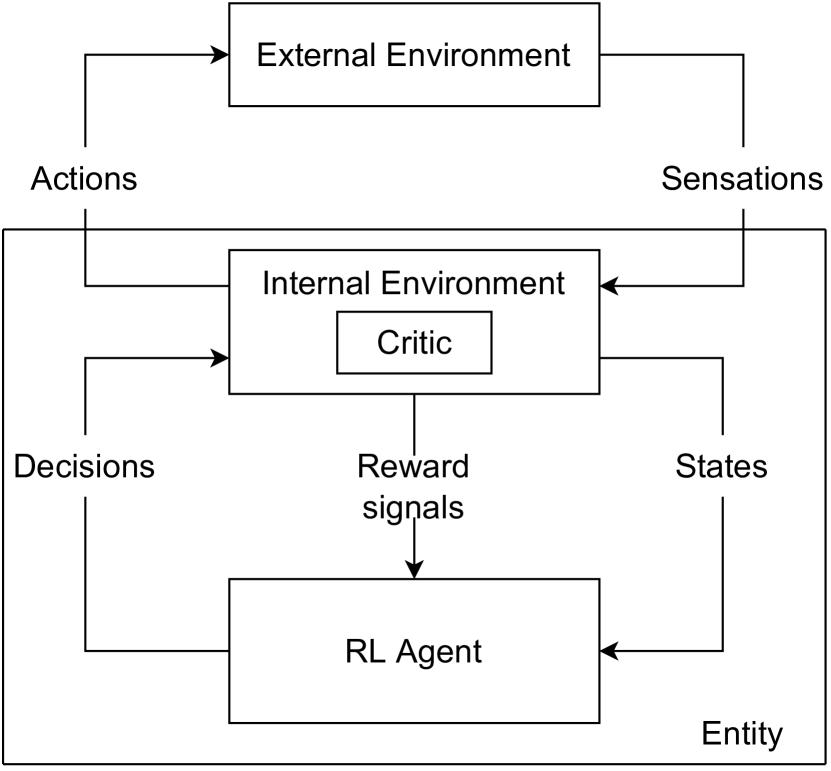
Figure 1. Model of RL integrating IM, taken in Singh et al. (2010). The environment is factored into an internal and external environment, with all reward coming from the former.

In addition, rather than considering the MDP environment as the environment in which the agent achieves its task, it suggests that the MDP environment can be formed of two parts: the external part which corresponds to the potential task and the environment of the agent; the internal part which computes the MDP states and the secondary reward signal using potentially previous interactions. Consequently, we can consider an intrinsic reward as a reward signal received from the MDP environment. The MDP state is no more the external state but an internal state of the agent. However, from now, we will follow the terminology of RL and the term reward will refer to the primary reward signal.

Figure 1 summarizes the framework: the critic is in the internal part of the agent, it computes the intrinsic reward and deals with the credit assignment. The agent can merge intrinsic rewards and extrinsic rewards in its internal part. The state includes sensations and any form of internal context; in this section we refer to this state as a contextual state. The decision can be a high-level decision decomposed by the internal environment into low-level actions.

This conceptual model incorporates intrinsic motivations into the formalism of MDP. Now, we will review how this model is instantiated in practice. Indeed it is possible to extend RL to incorporate the three new components that are intrinsic rewards, high-level decisions and contextual states. We separately study them in the following sections.

2.4. Intrinsic rewards and information theory

Throughout our definition of intrinsic motivation, one can notice that the notion of information comes up a lot. This is not hazardous and quantifying information proves useful to generate intrinsic rewards. In this section, we provide the basics about information theory and explain how to combine intrinsic and extrinsic rewards. However, we emphasize that intrinsic rewards are not restricted to information measures and their characterization mostly depends on whether the reward function fits the properties of an intrinsic motivation.

The Shannon entropy quantifies the mean necessary information to determine the value of a random variable. Let $X$ be a random variable with a law of density $p(X)$ satisfying the normalization and positivity requirements, we define its entropy by:

(5) $$H(X)=-\int_{X}p(x)\log p(x)dx.$$

In other words, it allows to quantify the disorder of a random variable. The entropy is maximal when $X$ follows a uniform distribution, and minimal when $p(X)$ is equal to zero everywhere except in one value, which is a Dirac distribution. From this, we can also define the entropy conditioned on a random variable $S$. It is similar to the classical entropy and quantifies the mean necessary information to find $X$ knowing the value of an other random variable $S$:

(6) $$H(X|S)=-\int_{S}p(s)\int_{X}p(x|s)\log p(x|s)dxds.$$

The mutual information allows to quantify the information contained in a random variable $X$ about an other random variable $Y$. It can also be viewed as the decrease of disorder brought by a random variable $Y$ on a random variable $X$. The mutual information is defined by:

(7) $$I(X;Y)=H(X)-H(X|Y)$$

We can notice that the mutual information between two independent variables is zero (since $H(X|Y)=H(X)$). Similarly to the conditional entropy, the conditional mutual information allows to quantify the information contained in a random variable about an other random variable, knowing the value of a third one. It can be written in various ways:

(8a) $$I(X;Y|S) =H(X|S)-H(X|Y,S)=H(Y|S)-H(Y|X,S)$$

(8b) $$=D_{KL}\Big{[}p(X,Y|S)||p(X|S)p(Y|S)\Big{]}$$

We can see with Equation 8a that the mutual information is symmetric and that it characterizes the decrease in entropy on X brought by Y (or inversely). Equation 8b defines the conditional mutual information as the Kullback-Leibler divergence (Cover and Thomas, 2012), noted $D_{KL}(.||.)$, between distribution $P(Y,X|S)$ and the same distribution if $Y$ and $X$ were independent variables (the case where $H(Y|X,S)=H(Y|S)$).

For further information on these notions, the interested reader can refer to Cover and Thomas (2012). Sections 5, 6, 7 illustrate how we can use information theory to reward an agent. In practice, there are multiple ways to integrate an intrinsic reward into a RL framework. The main approach is to compute the agent’s reward $r$ as a weighted sum of an intrinsic reward $r_{int}$ and an extrinsic reward $r_{ext}$: $r=\alpha r_{int}+\beta r_{ext}$ (Kakade and Dayan, 2002; Burda et al., 2018). Of course, one of the weighting coefficient $\alpha$ and $\beta$ can be set to 0.

2.5. Decisions and hierarchical RL

Hierarchical reinforcement learning (HRL) architectures are adequate candidates to model the decision hierarchy of an agent (Barto and Mahadevan, 2003; Dayan and Hinton, 1993; Sutton et al., 1999). Dayan and Hinton (1993) introduced the feudal hierarchy, called Feudal reinforcement learning. In this framework, a manager selects the goals that workers will try to achieve by selecting low-level actions. Once the worker achieved the goal, the manager can select an other goal, so that the interactions keep going. The manager rewards the RL-based worker to guide its learning process; we formalize this with intrinsic motivation in the next section. Below, Figure 3 illustrates the use of a hierarchical decision in contrast with the use of low-level actions. At the origin, the hierarchical architectures have been introduced to make easier the long-term credit assignment (Dayan and Hinton, 1993; Sutton et al., 1999). This problem refers to the fact that rewards can occur with a temporal delay and will only very weakly affect all temporally distant states that have preceded it, although these states may be important to obtain that reward. Indeed, the agent must propagate the reward along the entire sequence of actions (through Equation 4) to reinforce the first involved state-action tuple. This process can be very slow when the action sequence is large. This problem also concerns determining which action is decisive for getting the reward, among all actions of the sequence. In contrast, if an agent can take advantage of temporally-extended actions, a large sequence of low-level actions become a short sequence of time-extended decisions that make easier the propagation of rewards.

This goal setting mechanism can be extended to create managers of managers so that an agent can recursively define increasingly abstract decisions as the hierarchy of RL algorithms increases. Relatively to Figure 1, the internal environment of a RL module becomes the lower level module. We can model these decisions as options. An option $op\in\mathcal{O}$ is defined through 3 components: 1- A set of starting states $\mathcal{I}\subset S$ from which an option can be applied; 2- A policy (or worker) that is responsible of achieving the options with lower-level actions. This is studied in the next section; 3- A completion function $\mathcal{F}$ that specifies the probability of completing the option in each state.

Typically, the starting state can derive from $d_{0}$ (all options start at the beginning of an episode) or the full set of states $S$ (options can start everywhere). The completion function can also set a probability $0$ everywhere (Eysenbach et al., 2018), in this case, it ends at the same time as an episode. Such specific cases often occur (Eysenbach et al., 2018). Options where originally learnt during a pre-training phase with exclusively extrinsic rewards (Sutton et al., 1999), it was meant to take advantage of expert knowledge on the task. However, in our framework, we are interested in intrinsically motivated agent, so, in the next section, we take a closer look on how to learn the policies that learn to achieve goals using intrinsic motivation. In particular, we will define goals, skills and explain how to build a contextual state.

2.6. Goal-parameterized RL

Usually, RL agents solve only one task and are not suited to learn multiple tasks. Thus, an agent is unable to generalize across different variants of a task. For instance, if an agent learns to grasp a circular object, it will not be able to grasp a square object. In the developmental model described in Section 2.3, the decisions can be hierarchically organized into several levels where an upper-level takes decision (or sets goals) that a lower-level has to satisfy. This questions: 1- how a DRL algorithm can make its policy dependent on the goal set by its upper-level decision module ? 2- How to compute the intrinsic reward using the goal ? These issues rise up a new formalism based on developmental machine learning (Colas et al., 2020).

In this formalism, a goal is defined by the pair $(g,R_{G})$ where $G\subset\mathbb{R}^{d}$, $R_{G}$ is a goal-conditioned reward function and $g\in G$ is the $d\text{-dimensional}$ goal embedding. This contrasts with the notion of task which is proper to an extrinsic reward function assigned by an expert to the agent. With such embedding, one can generalize DRL to multi-goal learning, or even to every available goal in the state space, with the Universal Value Function Approximator (UVFA) (Schaul et al., 2015). UVFA integrates, by concatenating, the state goal embedding $g$ with the state of the agent to create a contextual state $c=(g,s)$. Depending on the semantic meaning of a skill, we can further enhance the contextual states with other actions or states executed after starting executing the skill (cf. Section 7).

We can now define the skill associated to each goal as the goal-conditioned policy $\pi^{g}(a|s)=\pi(a|g,s)$; in other words, a skill refers to the sensorimotor mapping that achieve a goal (Thill et al., 2013). This skill may by learnt or unlearnt according to the expected intrinsic rewards it gathers. It implies that, if the goal space is well-constructed (as often a ground state space for example, $R_{G}=S$), the agent can generalize its policy across the goal space, i.e the corresponding skills of two close goals are similar. For example, let us consider an agent moving in a closed maze where every position in the maze can be a goal. We can set $G=S$ and set the intrinsic reward function to be the euclidean distance between the goal and the current state of the agent $R_{G}:S\times G\rightarrow\mathbb{R},(s,g)\rightarrow||s-g||_{2}$.

This formalism completes the instantiation of the architectures described in Section 2.3. Now we will explain how, in practice, one can efficiently learn the goal-conditioned policy.

2.7. Efficient learning with goal relabelling

When the goal space is a continuous state space, it is difficult to determine whether a goal is reached or not, since two continuous values are never exactly equal. Hindsight experience replay (HER) (Andrychowicz et al., 2017) tackles this issue by providing a way to learn on multiple objectives with only one interaction. With author’s method, the agent can use an interaction done to accomplish one goal to learn on an other goal, by modifying the associated intrinsic reward. This mechanism greatly improves the sample efficiency since it avoids to try all interactions for every goals.

Let us roll out an example. An agent acts in the environment to gather a tuple $(s,s^{\prime},r_{g},a,g)$ where $r_{g}$ is the reward associated to the goal $g$. The agent can learn on this interaction, but can also use this interaction to learn other goals; to do so, it can change the goal into a new goal and recompute the reward, resulting in a new interaction $(s,s^{\prime},r_{g^{\prime}},a,g^{\prime})$. The only constraint for doing this is that the reward function $R(s,a,s^{\prime},g^{\prime})$ has to be known, which is the case with an intrinsic reward function. Typically, an agent can have a goal state and a reward function which is $1$ if it is into that state and $0$ otherwise. At every interaction, it can change its true goal state for its current state and learn with a positive reward.

3. Challenges of DRL

In this section, we detail two main challenges of current DRL methods that are partially addressed by IMs.

3.1. Sparse rewards

Classic RL algorithms operate in environments where the rewards are dense, i.e. the agent receives a reward after almost every completed action. In this kind of environment, naive exploration policies such as $\epsilon$-greedy (Sutton and Barto, 1998) or the addition of a Gaussian noise on the action (Lillicrap et al., 2015) are effective. More elaborated methods can also be used to promote exploration, such as Boltzmann exploration (Cesa-Bianchi et al., 2017; Mnih et al., 2015) or an exploration in the parameter-space (Plappert et al., 2017; Rückstiess et al., 2010; Fortunato et al., 2017). In environments with sparse rewards, the agent receives a reward signal only after it executed a large sequence of specific actions. The game Montezuma’s revenge (Bellemare et al., 2015) is a benchmark illustrating a typical sparse reward function. In this game, an agent has to move between different rooms while picking up objects (it can be keys to open doors, torches, …). The agent receives a reward only when it finds objects or when it reaches the exit of the room. Such environments with sparse rewards are almost impossible to solve with the above mentioned undirected exploration policies (Thrun, 1992) since the agent does not have local indications on the way to improve its policy. Thus the agent never finds rewards and cannot learn a good policy with respect to the task (Mnih et al., 2015). Figure LABEL:im:sparse_reward illustrates the issue on a simple environment.

This issue stresses out the need for directed exploration methods (Thrun, 1992). While intrinsic motivation can provide such direction, the principle of ”optimism in face of uncertainty” (Audibert et al., 2007) can also execute a directed exploration without intrinsic motivation (Thrun, 1992). Briefly, this principle can incite agents to go in areas with a lot of epistemic uncertainties about its Q-values (Ciosek et al., 2019; Pacchiano et al., 2020). Yet, it is hard to approximate the epistemic uncertainty and it only slightly improves exploration (Ciosek et al., 2019). This principle can also relate with some intrinsic motivations when we consider uncertainty about models (see Section 5.3).

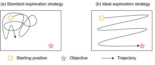
Figure 2. Example of a very simple sparse reward environment, explored by two different strategies. The agent, represented by a circle, strives to reach the star. The reward function is one when the agent reaches the star and zero otherwise. (a) the agent explores with standard methods such as $\epsilon\text{-greedy}$; as a result, it stays in its surrounded area because of the temporal inconsistency of its behaviour. (b) we imagine an ideal exploration strategy where the agent covers the whole state space to discover where rewards are located. The fundamental difference between the two policies is the volume of the state space explored for a given time.

Rather than working on an exploration policy, it is common to shape an intermediary dense reward function that adds to the reward associated to the task in order to make the learning process easier for the agent (Su et al., 2015). However, the building of a reward function often reveals several unexpected errors (Ng et al., 1999; Amodei et al., 2016) and most of the time requires expert knowledge. For example, it may be difficult to shape a local reward for navigation tasks. Indeed, one has to be able to compute the shortest path between the agent and its goal, which is the same as solving the navigation problem. On the other side, the automation of the shaping of the local reward (without calling on an expert) requires too high computational resources (Chiang et al., 2019). We will see in Section 5, 6 and 7 how IM is a valuable method to encourage exploration in a sparse rewards setting.

3.2. Temporal abstraction of actions

As argued in Section 2.5, skills, through hierarchical RL, are a key element to speed up the learning process since the number of decisions to take is significantly reduced when skills are used. In particular, they make easier the credit assignment. Skills can be manually defined, but it requires some extra expert knowledge (Sutton et al., 1999). To avoid providing hand-made skills, several works proposed to learn them with extrinsic rewards (Bacon et al., 2017; Li et al., 2020). However, if an agent rather learns skills in a bottom-up way, i.e with intrinsic rewards rather than extrinsic rewards, learnt skills become independent from possible tasks. This way, skills can be reused across several tasks to improve transfer learning (Aubret et al., 2020; Heess et al., 2016) and an agent can learn skills even though it does not access rewards, improving exploration when rewards are sparse (Machado et al., 2017). Let us illustrate both advantages.

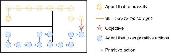
Figure 3. Example of two policies in a simple environment, one uses skills (yellow), the other one only uses primitive actions (blue). Agents have to reach the star.

Exploration when rewards are sparse.

Figure 3 illustrates the benefit in terms of exploration when an agent hierarchically uses skills. The yellow agent can use a skill Go to the far right, to reach the rewarding star while the blue agent can only use low-level cardinal movements. The problem of exploration becomes trivial for the agent using skills, since one exploratory action can lead to the reward. In contrast, it requires an entire sequence of specific low-level actions for the other agent to find the reward. This problem arises from the minimal number of specific actions needed to get a reward (see also Section 3.1). A thorough analysis of this aspect can be found in (Nachum et al., 2019b).

Reusing skills across several tasks.

Skills learnt with intrinsic rewards are not specific to a task. Assuming an agent is required to solve several tasks in a similar environment, i.e a single MDP with a changing extrinsic reward function, an agent can execute its discovered skills to solve all tasks. Typically, in Figure 3, if both agents learnt to reach the star and we move the star somewhere else in the environment, the yellow agent would still be able to execute Go to the far right and executing this skill may make the agent closer to the new star. In contrast, the blue agent would have to learn a whole new policy. In Section 7, we provide insights on how an agent can discover skills in a bottom-up way.

4. Classification of methods

In order to tackle the problem of exploration, an agent may want to identify and return in rarely visited states or unexpected states, which can be quantified with current intrinsic motivations. We will particularly focus on two objectives that address the challenge of exploring with sparse rewards, each with different properties: maximizing novelty and surprise. Surprise and novelty are specific notions that have often been used in an interchanged way and we are not aware of a currently unanimous definition of novelty (Barto et al., 2013). The third notion we study, skill learning, focuses on the issue of skill abstraction. In practice, surprise and novelty are currently maximized as a flat intrinsic motivation, i.e without using hierarchical decisions. This mostly helps to improve exploration when rewards are sparse. In contrast, skill learning allows to define time-extended hierarchical skills that enjoy all the benefits argued in Section 3.2.

Table 1 sums up our taxonomy. based on information theory that reflects the high-level studied concepts of novelty, surprise and skill learning. In practice, we mostly take advantage of the mutual information to provide a quantity for our conceptual objectives. These objectives are compatible with each other and may be used simultaneously, as argued in Section 8.3. Within each category of objectives, we additionally highlight several ways to maximize each objective and provide details about the underlying methods of the literature. We sum up the methods in Tables 2, 3 and 4 and compare their respective advantages when possible.

Surprise: $I(S^{\prime};\Phi_{T}|h,S,A)$, Section 5
Formalism	Information gain	Information gain	Information gain
	over forward model	over the true model	over density model
Sections	Section 5.3	Section 5.2	Section 5.4
Rewards	$D_{KL}(p(\Phi|h,s,a,s^{\prime})||p(\Phi|h))$	$||s^{\prime}-\hat{s}^{\prime}||_{2}^{2}$	$\frac{1}{\sqrt{\hat{N}(s^{\prime})}}$
Advantage	Simplicity	Stochasticity robustness	Good exploration
Novelty: $I(S;Z)$, Section 6
Formalism	Parametric density	K-nearest neighbors
Sections	Section 6.1	Section 6.2
Rewards	$-\log\rho(s^{\prime})$	$\log(1+\frac{1}{K}\sum_{0}^{K}||f(s^{\prime})-nn_{k}(f(S_{b}),f(s^{\prime}))||_{2})$
Advantage	Good exploration	Best exploration
Skill learning: $I(G;u(\mathcal{T}))$, Section 7
Formalism	Fixed goal distribution	Goal-state	Proposing diverse goals
		achievement
Sections	Section 7.1	Section 7.2	Section 7.3
Rewards	$\log p(g|s^{\prime})$	$-||s_{g}-s^{\prime}||_{2}^{2}$	$(1+\alpha_{skew})\log p(s_{g})$
Advantage	Simple goal sampling	High-granularity skills	More diverse skills

Table 1. Summary of our taxonomy of intrinsic motivations in DRL. The function $u$ outputs a part of the trajectories $\mathcal{T}$, $Z$ and $G$ are internal random variables respectively denoting state representations and self-assigned goals. Please, refer to the corresponding sections for more details about methods and notations. The reward function aims to represent the one used in the category.

5. Surprise

In this section, we study methods that maximize the surprise. Firstly, we formalize the notions of surprise, then we will study three approaches for computing intrinsic rewards based of these notions.

5.1. Definition of surprise

In this section, we assume the agent learns either a density model (Section 5.4) or a forward model of the environment (Sections 5.3 and 5.2) parameterized by $\phi\in\Phi$. The density model induces a marginal distribution of state $p(S|\phi)$ and a forward model computes the next-state distribution conditioned on a tuple state-action $p(S^{\prime}|S,A,\phi)$. Typically, this can be the parameters of a neural network. Trying to approximate the true model, the agent maintains an approximate distribution $p(\Phi|h)$ of models, where $h_{t}=h$ refers to the ordered history of interactions $((s_{0},a_{0},s_{1}),(s_{1},a_{1},s_{2}),\dots,(s_{t-1},a_{t-1},s_{t}))$. In this section, $h$ simulates a dataset of interactions, we use it to clarify the role of the dataset. It is important to notice that the policy feeds this $h$.

In this case, surprise quantifies the mismatch between an expectation and the true experience of an agent (Barto et al., 2013; Ekman and Davidson, 1994). In this paper, we refer to the definition of Itti and Baldi (2009), which define it as the discrepancy between a prior distribution of beliefs and the posterior probability distribution following an observation (Itti and Baldi, 2009; Storck et al., 1995). If an agent maximizes the surprise over a model through interactions with the environment, which is often the case (Barto et al., 2013), it leads to the expected information gain objective (Sun et al., 2011). Intuitively, the agent returns in states where it experienced an unexpected transition. Using the KL-divergence to assess the discrepancy, surprise can be computed as $D_{KL}(p(\Phi|h_{t+1})||p(\Phi|h_{t}))$ where $\phi\in\Phi$ are parameters of a model and $t$ denotes the timestep.

In this case, the agent has a prior distribution about model parameters $p(\Phi)$ and this model can be updated using the Bayes rule:

(9) $$p(\phi|h,s,a,s^{\prime})=\frac{p(\phi|h)\;p(s^{\prime}|h,s,a,\phi)}{p(s^{\prime}|h,s,a)}.$$

Information gain over agent’s model.

The expected information gain (Sun et al., 2011; Little and Sommer, 2013) over a forward or density model parameterized by $\phi$ can be formulated as:

(10a) $$IG(h,A,S^{\prime},S,\Phi) =I(S^{\prime};\Phi|h,A,S)=\mathbb{E}_{\begin{subarray}{c}(s,a)\sim p(\cdot|h)\\ s^{\prime}\sim p(\cdot|s,a,h)\end{subarray}}D_{KL}(p(\Phi|h,s,a,s^{\prime})||p(\Phi|h))$$

(10b) $$\approx\mathbb{E}_{\begin{subarray}{c}(s,a)\sim\pi\\ s^{\prime}\sim p(\cdot|s,a,h,\phi_{T})\end{subarray}}D_{KL}(p(\Phi|h,s,a,s^{\prime})||p(\Phi|h))$$

Actively maximizing the expected information gain amounts to reduce the uncertainty of the model. We emphasize that $p(\phi|h)=p(\phi|h,a,s)$ since only full transitions provide information about the true dynamics of the environment. In this case, $p(s^{\prime}|s,a,h)$ does not refer to the probability induced by the environment, but rather to the probability induced by the current history of transitions. This is stressed out by writing:

(11) $$p(s^{\prime}|s,a,h)=\sum_{\phi\in\Phi}p(s^{\prime}|s,a,h,\phi)p(\phi|s,a,h).$$

We highlight that the difference between Equation 10a and Equation 10b is important and misleading in the literature (Houthooft et al., 2016; Little and Sommer, 2013; Sun et al., 2011): in the first equation, the agent imagines new outcomes in order to select actions that maximize the change in the internal model, while in Equation 10b, the agents acts and uses the new states to update its model.

Information gain over the true forward model.

In our formalism, we assume that there is a distribution of true models $p(\Phi_{T})$ that underpins the transition function of the environment $T$. In contrast with $\Phi$, this is a property of the environment. One can see this distribution as a Dirac distribution if only one model exists or as a categorical distribution of several forward models. We define the expected information gain over the true models as:

(12a) $$IG(h,A,S^{\prime},S,\Phi_{T}) =I(S^{\prime};\Phi_{T}|h,A,S)=H(\Phi_{T}|h,A,S)-H(\Phi_{T}|h,A,S,S^{\prime})$$

(12b) $$=\mathbb{E}_{\begin{subarray}{c}(s,a)\sim p(\cdot|h),\,\phi_{T}\sim p(\cdot)\\ s^{\prime}\sim p(\cdot|s,a,\phi_{T})\end{subarray}}\log p(s^{\prime}|s,a,h,\phi_{T})-\log p(s^{\prime}|s,a,h).$$

Maximizing Equation 12b amounts to look for states that provides new information about the true models distribution. We can see that the left-hand side of Equation 12b incites the agent to target inherently deterministic areas, i.e, given the true forward model, the agent would exactly know where it ends up. At the opposite, the right-hand term pushes the agent to go in stochastic areas according to its current knowledge. Overall, to improve this objective, an agent has to reach areas that are more deterministic than what it thinks they are. One can see that, assuming $p(s^{\prime}|s,a,h,\phi_{T})\approx p(s^{\prime}|s,a,\phi,h)$, one falls back on the expected information gain (see also Equation 20b). In contrast with Equation 10b, this objective takes advantage of the true model, which is most of the time unknown, thereby making the objective hardly tractable. As such, in this perspective, surprise results from an agent-centric approximation of the discrepancy between the agent’s model and the environment model.

In the following, we will study three objectives: the expected information gain over the true forward models, the expected information gain over the forward model and the expected information gain over density models.

5.2. Information gain over the true forward model

To avoid the need of the true forward model, the agent can omit the left-hand term of Equation 12b by assuming the true forward model is modelled as a deterministic forward model. In this case, we can write:

(13a) $$I(S^{\prime};\Phi_{T}|h,A,S) \propto\mathbb{E}_{\begin{subarray}{c}(s,a)\sim p(\cdot|h),\phi_{T}\sim p(\cdot)\\ s^{\prime}\sim p(\cdot|s,a,\phi_{T})\end{subarray}}-\log p(s^{\prime}|s,a,h)$$

(13b) $$=\mathbb{E}_{\begin{subarray}{c}(s,a)\sim p(\cdot|h),\,\phi_{T}\sim p(\cdot)\\ s^{\prime}\sim p(\cdot|s,a,\phi_{T})\end{subarray}}-\log\sum_{\phi\in\Phi}p(s^{\prime}|h,s,a,\phi)p(\phi|h)$$

(13c) $$\geq\mathbb{E}_{\begin{subarray}{c}\phi_{T}\sim p(\cdot),\,(s,a)\sim p(\cdot|h)\\ s^{\prime}\sim p(\cdot|s,a,\phi_{T}),\phi\sim p(\cdot|h)\end{subarray}}-\log p(s^{\prime}|h,s,a,\phi)$$

where we applied the Jensen inequality in Equation 13c and $\phi_{T}\sim p(\cdot)$ is fixed. One can model $p(s^{\prime}|h,s,a,\phi)$ with a unit-variance Gaussian distribution in order to obtain a tractable loss. This way, we have:

(14a) $$\mathbb{E}_{\begin{subarray}{c}(s,a)\sim p(\cdot|h),\,\phi_{T}\sim p(\cdot)\\ s^{\prime}\sim p(\cdot|s,a,\phi_{T}),\,\phi\sim p(\cdot|h)\end{subarray}}-\log p(s^{\prime}|\phi,h,a,s) \approx\mathbb{E}_{\begin{subarray}{c}(s,a)\sim p(\cdot|h),\,s^{\prime}\sim p(\cdot|s,a,\phi_{T})\\ \phi\sim p(\cdot|h),\,\phi_{T}\sim p(\cdot)\end{subarray}}-\log\frac{1}{(2\pi)^{d/2}}e^{-0.5(s^{\prime}-\hat{s}^{\prime})^{T}(s^{\prime}-\hat{s}^{\prime})}$$

(14b) $$\propto\mathbb{E}_{\begin{subarray}{c}(s,a)\sim p(\cdot|h),\,s^{\prime}\sim p(\cdot|s,a,\phi_{T})\\ \phi\sim p(\cdot|h),\,\phi_{T}\sim p(\cdot)\end{subarray}}||s^{\prime}-\hat{s}^{\prime}||_{2}^{2}+Const$$

where

(15) $$\hat{s}^{\prime}=\underset{s^{\prime\prime}\in S}{\operatorname{arg}\,\operatorname{max}}\;p(s^{\prime\prime}|h,a,s,\phi)$$

represents the mean prediction and $\phi$ parameterizes a deterministic forward model. Following the objective, we can extract a generic intrinsic reward as:

(16) $$R(s,a,s^{\prime})=||f(s^{\prime})-f(\hat{s}^{\prime})||_{2}^{2}$$

where $f$ is a generic function (e.g. identity or a learnt one) encoding the state space into a feature space. Equation 16 amounts to reward the predictor error of $\phi$ in the representation $f$. In the following, we will see that learning a relevant function $f$ is the main challenge.

The first natural idea to test is whether a function $f$ is required. Burda et al. (2019) learn the forward model from the ground state space and observe it is inefficient when the state space is large. In fact, the euclidean distance is meaningless in such high-dimensional state space. In contrast, they raise up that random features extracted from a random neural network can be very competitive with other state-of-art methods. However they poorly generalize to environment changes. An other model, Dynamic Auto-Encoder (Dynamic-AE) (Stadie et al., 2015), computes the distance between the predicted and the real state in a state space compressed with an auto-encoder (Hinton and Salakhutdinov, 2006). $g$ is then the encoding part of the auto-encoder. However this approach only slightly improves the results over Boltzmann exploration on some standard Atari games. Other works also consider a dynamic-aware representation (Ermolov and Sebe, 2020). These methods are unable to handle the local stochasticity of the environment (Burda et al., 2019). For example, it turns out that adding random noise in a 3D environment attracts the agent; it passively watches the noise since it is unable to predict the next observation. This problem is also called the white-noise problem (Pathak et al., 2017; Schmidhuber, 2010). This problem emerges by considering only the right-hand term of Equation 12b, making the agent assumes environments are deterministic. Therefore, exploration with prediction error breaks down when this assumption is no longer true.

To tackle exploration with local stochasticity, the intrinsic curiosity module (ICM) (Pathak et al., 2017) learns a state representation function $f$ end-to-end with an inverse model (i.e. a model which predicts the action done between two states). Thus, the function $f$ is constrained to represent things that can be controlled by the agent during next transitions. Secondly, the forward model used in ICM predicts, in the feature space computed by $f$, the next state given the action and the current state. The prediction error does not incorporate the white-noise that does not depend on actions, so it will not be represented in the feature state space. ICM notably allows the agent to explore its environment in the games VizDoom and Super Mario Bros. Building a similar action space, Exploration with Mutual Information (EMI) (Kim et al., 2019a) significantly outperforms previous works on Atari but at the cost of several complex layers. EMI transfers the complexity of learning a forward model into the learning of states and actions representation through the maximization of $I([S,A];S^{\prime})$ and $I([S,S^{\prime}];A)$. Then, the forward model $\phi$ is constrained to be a simple linear model in the representation space. Furthermore, EMI introduces a model error which offloads the linear model when a transition remains strongly non-linear (such as a screen change). However one major drawback of ICM and EMI is the incapacity of their agent to keep in their representation what depends on their long-term control. For instance, in a partially observable environment, an agent may perceive the consequences of its actions several steps later. In addition they remain sensitive to stochasticity when it is produced by an action (Burda et al., 2019).

An other way to tackle local stochasticity can be to maximize the improvement of prediction error, or learning progress, of a transition model (Schmidhuber, 1991; Azar et al., 2019; Lopes et al., 2012; Oudeyer et al., 2007; Kim et al., 2020). One can see this as approximating the left-hand side of Equation 12b with:

(17) $$\log p(s^{\prime}|s,a,h,\phi_{T})-\log p(s^{\prime}|s,a,h) \approx\log p(s^{\prime}|s,a,h^{\prime})-\log p(s^{\prime}|s,a,h)$$

where $h^{\prime}$ concatenates $h$ with an arbitrary number of additional interactions. As $h^{\prime}$ becomes large enough and the agent updates its forward model, its forward model converges to the true transition model. Formally, if one stochastic forward model can describe the transitions, we can write:

$$\lim_{|h^{\prime}|\rightarrow\inf}p(s^{\prime}|s,a,h^{\prime}) =\lim_{|h^{\prime}|\rightarrow\inf}\sum_{\Phi}p(s^{\prime}|s,a,h^{\prime},\phi)p(\phi|h^{\prime})$$

(18a) $$=p(s^{\prime}|s,a,h^{\prime},\phi_{T})$$

In practice, we can not wait for discovering a long sequence of new interactions and the reward can be dependent on a small set of interactions and the efficiency of the gradient update of the forward model. Yet, the theoretical connection with the true expected information gain may indeed explain the robustness of learning progress to stochasticity (Linke et al., 2020).

Conclusion.

While these methods perform well in deterministic environments, they struggle to offset the determinism assumption that underpines the focus on Equation 13a; it results that standard methods focus on the more stochastic areas. Methods that tackle stochasticity may not predict important long-term information about the environment or they need to compute a learning progress measure, which is non-trivial.

5.3. Information gain over forward model

In this subsection, we study the works that maximize the expected information gain over forward models. Here, $\phi$ are parameters of a learnt forward model. Using Equation 10b, we can extract an intrinsic reward:

(19) $$R(s,a,s^{\prime})=D_{KL}(p(\Phi|h,s,a,s^{\prime})||p(\Phi|h)).$$

This way, an agent executes actions that provide information about the dynamics of the environment. This allows, on one side, to push the agent towards areas it does not know, and on the other side to prevent attraction towards stochastic areas. Indeed, if the area is deterministic, environment transitions are predictable and the uncertainty about its dynamics can decrease. At the opposite, if transitions are stochastic, the agent turns out to be unable to predict transitions and does not reduce uncertainty. The exploration strategy VIME (Houthooft et al., 2016) computes this intrinsic reward by modelling $p(\phi|h)$ with Bayesian neural networks (Graves, 2011). The interest of Bayesian approaches is to be able to measure the uncertainty of the learned model (Blundell et al., 2015). This way, assuming a fully factorized Gaussian distribution over model parameters, the KL-divergence has a simple analytic form (Houthooft et al., 2016; Linke et al., 2020), making it easy to compute. However, the interest of the proposed algorithm is shown only on simple environments and the reward can be computationally expensive to compute. Achiam and Sastry (2017) propose a similar method (AKL), with comparable results, using deterministic neural networks, which are simpler and quicker to apply. The weak performance of both models is probably due to the difficulty to retrieve the uncertainty reduction by rigorously following the mathematical formalism of information gain.

The expected information gain can also be written:

$$I(S^{\prime};\Phi|h,A,S) =H(S^{\prime}|h,A,S)-H(S^{\prime}|A,\Phi,S,h)$$

(20a) $$\approx-\mathbb{E}_{\begin{subarray}{c}(s,a)\sim p(\cdot|h),\,\phi_{T}\sim p(\cdot)\\ s^{\prime}\sim p(\cdot|s,a,h,\phi_{T})\end{subarray}}\log p(s^{\prime}|h,s,a)+\mathbb{E}_{\begin{subarray}{c}\phi\sim p(\cdot|h,s,a,s^{\prime})\\ (s,a)\sim p(\cdot|h),s^{\prime}\sim p(\cdot|s,a,h,\phi_{T})\end{subarray}}\log p(s^{\prime}|s,a,\phi,h)$$

(20b) $$=\mathbb{E}_{\begin{subarray}{c}\phi\sim p(\cdot|h,s,a,s^{\prime}),\,\phi_{T}\sim p(\cdot)\\ (s,a)\sim p(\cdot|h),s^{\prime}\sim p(\cdot|s,a,h,\phi_{T})\end{subarray}}-\log\sum_{\phi\in\Phi}p(s^{\prime}|\phi,h,s,a)p(\phi|h)+\log p(s^{\prime}|s,a,\phi,h)$$

Using similar equations than in Equation 20b, in JDRX (Shyam et al., 2019), authors show that one can maximize the information gain by computing the Jensen-Shannon or Jensen-Rényi divergence between distributions of states induced by several forward models. The more the models are trained on a state-action tuple, the more they will converge to the expected distribution of next states. Intuitively, the reward represents how much the different transition models disagree on the next-state distribution. Other works also maximize a similar form of disagreement (Pathak et al., 2019; Yao et al., 2021; Sekar et al., 2020) by looking at the variance of predictions among several learnt transition models. While these models handle the white-noise problem, the main intrinsic issue is computational since they require multiple forward models to train.

Conclusion.

Despite the theoretical power of the information gain for improving exploration, it remains hard to efficiently estimate it and use it in difficult tasks.

5.4. Information gain over density model

Surprise can also arise by quantifying the discrepancy between its probability of occurring and the fact that it actually occurred (Barto et al., 2013). To quantify this probability of occuring, in this paragraph, we assume the agent tries to learn a density model $\phi\in\Phi$ that approximates the current marginal density distribution of states $p(s^{\prime})$. In this setting, we can define the expected information gain over a density model $\rho$ (Bellemare et al., 2016):

(21) $$IG(h,S,A,S^{\prime},\mathrm{P}) \approx\mathbb{E}_{\begin{subarray}{c}(s,a)\sim p(\cdot|h),\,\rho_{T}\sim p(\cdot)\\ s^{\prime}\sim p(\cdot|s,a,h,\mathrm{P}_{T})\end{subarray}}D_{KL}(p(\rho|h,s^{\prime})||p(\rho|h)).$$

We hypothesize that the adversarial training that results from the objective (active maximization of the KL-divergence and density fitting) results in an approximately uniform distribution of states (and a uniform density estimation). This may be due to the convexity of the KL-divergence in $p(\rho|h,s^{\prime})$ and $p(\rho|h)$ but we leave the proof to future work. To our knowledge, no works directly optimize this objective, but it has been shown that the information gain lower-bounds the squared inverse pseudo-count objective (Bellemare et al., 2016), which derives from count-based objectives; in the following, we will review count and pseudo-count objectives.

To efficiently explore its environment, an agent can count the number of times it visits a state and returns in rarely visited states. Such methods are said to be count-based (Strehl and Littman, 2008). As the agent visits a state, the intrinsic reward associated with this state decreases. It can be formalized with:

(22) $$R(s,a,s^{\prime})=\frac{1}{\sqrt{N(s^{\prime})}}$$

where $N(s)$ is the number of times that the state $s$ has been visited. Although this method is efficient and tractable in a tabular environment (with a discrete state space), it hardly scales when states are numerous or continuous since an agent never really returns in the same state. A first solution proposed by Tang et al. (2017), called TRPO-AE-hash, is to hash the latent space of an auto-encoder fed with states. However, these results are only slightly better than those obtained with a classic exploration policy. An other line of works propose to adapt counting to high-dimensional state spaces via pseudo-counts (Bellemare et al., 2016). Essentially, pseudo-counts allow the generalization of the count from a state towards neighbourhood states using a learnt density model $\rho$. This is defined as:

(23) $$\hat{N}(s^{\prime})=\frac{p(s^{\prime}|\rho)(1-p(s^{\prime}|\rho^{\prime})}{p(s^{\prime}|\rho^{\prime})-p(s^{\prime}|rho)}$$

where $\rho^{\prime}(s)$ computes the density of $s$ after having learnt on $s$. In fact, Bellemare et al. (2016) show that, under some assumptions, pseudo-counts increase linearly with the true counts. In this category, DDQN-PC (Bellemare et al., 2016) and DQN-PixelCNN (Ostrovski et al., 2017) compute $\phi$ using respectively a Context-Tree Switching model (CTS) (Bellemare et al., 2014) and a Pixel-CNN density model (Van den Oord et al., 2016). Although the algorithms based on density models work on environments with sparse rewards, they add an important complexity layer (Ostrovski et al., 2017). One can preserve the quality of observed exploration while decreasing the computational complexity of the pseudo-count by computing it in a learnt latent space (Martin et al., 2017).

There exists several other well-performing tractable exploration methods like RND (Burda et al., 2018), DQN+SR (Machado et al., 2020), RIDE (Raileanu and Rocktaschel, 2020) or BeBold (Zhang et al., 2020a). These papers argue the reward they propose more or less relate to a visitation count estimation.

Conclusion.

Maximizing the information gain over a density model may maximize the pseudo-count, which relates to count-based objectives. They provide interesting feedbacks for exploration, but in practice, pseudo-counts are hard to approximate since they rely on a powerfull density model, a strict online estimation of density and they assume $p(s|\phi)$ strictly increases $\forall s\in S$ (Ostrovski et al., 2017). In addition, they also struggle with the problem of randomness. For instance, let us assume that one (state, action) tuple can lead to two very different states with 50% chance each. The algorithm will manage to count for both states the number of visits, although it would take twice as long to avoid to be too much attracted. However, these methods do not address the white-noise problem since next states may be randomly generated at every steps. In this case, it is unclear how these methods could resist the temptation of going into this area since the counting associated to this state will never increase.

5.5. Conclusion

Method	Stoch	Computational cost	Montezuma’s Revenge
			Score	Steps
Information gain over the true forward model
PE with pixels (Burda et al., 2019)	No	HD FM	$\sim 160$	200M
Dynamic-AE (Stadie et al., 2015)	No	FM, AE	$0$	5M
PE with random features (Burda et al., 2019)	No	FM, RE	$\sim 250$	100M
PE with VAE features (Burda et al., 2019)	No	FM, VAE	$\sim 450$	100M
PE with ICM features (Burda et al., 2019)	$\sim$Yes	FM, Inverse model	$\sim 160$	100M
(Kim et al., 2019a)			$161$	50M
EMI (Kim et al., 2019a)	$\sim$Yes	Large architecture	$387$	50M
		Error model
PE with LWM (Ermolov and Sebe, 2020)	n/a	Whitened CL, FM	$2276$	50M
Learning progress (Schmidhuber, 1991; Azar et al., 2019)	Yes	Two forward errors	n/a	n/a
(Lopes et al., 2012; Oudeyer et al., 2007; Kim et al., 2020)
Information gain over density model
TRPO-AE-hash (Tang et al., 2017)	No	SimHash, AE	$75$	50M
DDQN-PC (Bellemare et al., 2016)	No	CTS	$3459$	100M
DQN-PixelCNN (Ostrovski et al., 2017)	No	PixelCNN	$1671$	100M
$\phi$-EB (Martin et al., 2017)	No	density model	$2745$	100M
DQN+SR (Machado et al., 2020)	n/a	Successor features	$1778$	20M
		HD FM
RND (Burda et al., 2018)	No	RE	$8152$	490M
(Machado et al., 2020)			$524$	100M
(Kim et al., 2019a)			$377$	50M
RIDE (Raileanu and Rocktaschel, 2020)	Yes	FM, Inverse model	n/a	n/a
		Pseudo-count
BeBold (Zhang et al., 2020a)	No	Hash table	$\sim 10000$	2000M
Information gain over forward model
VIME (Houthooft et al., 2016)	Yes	Bayesian FM	n/a	n/a
AKL (Achiam and Sastry, 2017)	Yes	Stochastic FM	n/a	n/a
Ensemble with random features (Pathak et al., 2019)	Yes	FMs, RE	n/a	n/a
Ensemble with observations (Yao et al., 2021)	Yes	FMs	n/a	n/a
Emsemble with PlaNet (Sekar et al., 2020)	Yes	FMs, PlaNet	n/a	n/a
JDRX (Shyam et al., 2019)	Yes	3 Stochastic FMs	n/a	n/a

• RE: Random encoder PE: Prediction error. HD: High-dimensional. NN: Neural network. Stoch: Stochasticity. FM: Forward model. CL: Contrastive loss. PlaNet: (Hafner et al., 2019a) RE: Random encoder.
  

• They only provide the number of frames in the paper, we assume they do not use frame skip.

• Result with one single seed.

Table 2. Comparison between different ways to maximize surprise. Stochasticity (Stoch) indicates whether the model handles the white-noise problem; $\sim$Yes means that the method may not handle the stochasticity generated by an action. Computational cost refers to highly expensive models added to standard RL algorithm. We also report the mean score on Montezuma’s revenge (Score) and the number of timesteps executed to achieve this score (Steps). We gathered results from the original paper and in other papers than the original one. Our table does not pretend to be an exhaustive comparison of methods but tries to give an intuition on their relative advantages.

We detailed three ways to define and maximize the surprise of an agent, based on the expected information gain over a true model of the environment.

Table 2 sums up all the surprise-based methods reviewed in this section, where it is also specified whether each method handles stochastic environments (Stoch) (cf. Section 5.2), and if expensive models are used (Computational Cost). The relative experimental advantage of each method is also reported in the Montezuma’s revenge environment (cf. Figure 4a)), a sparse-reward benchmark widely used to assess the ability of the method to explore. This gives a clue on how each method compare to the others. Methods categorized in information gain over forward model elegantly handle stochasticity from the environment, but usually apply in environments much simpler than Montezuma’s revenge. We can make a similar observation with methods based on learning progress. Methods based on prediction error achieve an overall low score on Montezuma’s Revenge, with stochasticity handling depending on the learnt latent space. PE with LWM (Ermolov and Sebe, 2020) achieves good performance, presumably because the learnt representation is more appropriate. One should be cautious about the low results of the Dynamic-AE (Stadie et al., 2015), because of the very low number of timesteps. Methods based on information gain over a density model are sensitive to stochasticity since nothing prevents them to return in noisy states, but achieve overall good results on Montezuma’s Revenge, thanks to the pseudo-count estimation. Among the best methods: BeBold (Zhang et al., 2020a) outstanding result has to be taken with caution, because it is not averaged over several seed; RND (Burda et al., 2018) is a simple method that achieves important asymptotic performance.

In practice, the expected information gain over a forward model and the learning progress well-approximate the expected information gain over the true model. Therefore, it appears that they intuitively and experimentally allow to well-explore inherently stochastic environments, but are hard to implement. The expected information gain over a density model can be seen as approximating the expected information gain over the true uniform density model. This makes the agent targets a uniform distribution of states: while it makes the agent sensitive to stochasticity, it executes robust exploration in deterministic environment. In fact, we discuss in the next section the relevance of aiming for a uniform distribution of states, through the study of novelty-based intrinsic motivations.

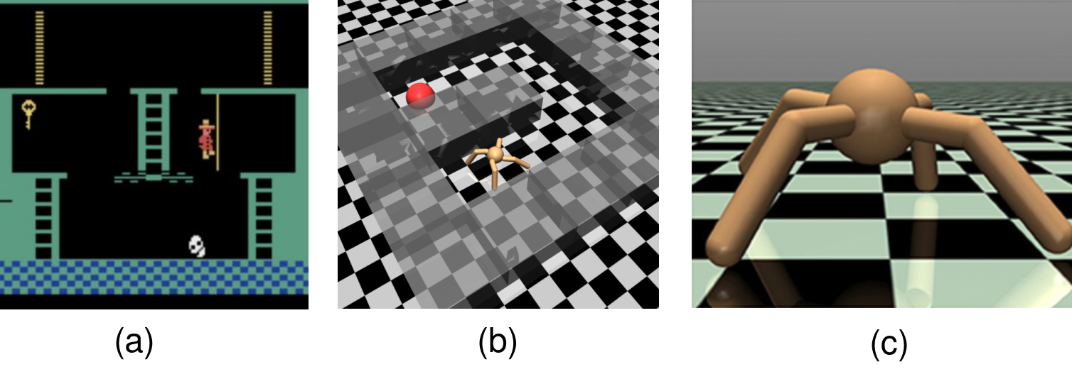
Figure 4. Different environments widely used in our reviewed papers. (a) Montezuma’s revenge, used to assess the ability of a policy to explore. (b) Ant maze (1x scale), used to evaluate the hierarchical organization of learnt skills (low-level: manipulation of low-level torques; high-level: navigation in the maze.) (c) Ant, used to analyse the diversity of learnt skills.

6. Novelty maximization

Novelty quantifies how much a stimuli contrasts with a previous set of experiences (Barto et al., 2013; Berlyne, 1966). More formally, Barto et al. (2013) defend that an observation is novel when a representation of it is not found in memory, or, more realistically, when it is not “close enough” to any representation found in memory. Previous experiences may be collected in a bounded memory or distilled in a learnt representation.

Several works propose to formalize novelty seeking as looking for low-density states (Becker-Ehmck et al., 2021), or similarly (cf. Section 6.2), states that are different from others (Lehman and Stanley, 2011; Conti et al., 2018). In our case, this would result in maximizing the entropy of a state distribution. This distribution can be the t-steps state distribution (cf. Equation 1) $H(d^{\pi}_{t}(S))$ or the entropy of the stationary state-visitation distribution over a horizon $T$:

(24) $$H(d^{\pi}_{0:T}(S))=H(\frac{1}{T}\sum_{t=1}^{T}d^{\pi}_{t}(S)).$$

In practice, these distributions can be approximated with a buffer. This formalization is not perfect and does not fit several intuitions about novelty (Barto et al., 2013). Barto et al. (2013) criticize such definition by stressing out that very distinct and memorable events may have low probabilities of occurring while not being novel (e.g a wedding). They suggest that novelty may rather relates to the acquisition of a representation of the incoming sensory data. Following this definition, we propose to formalize novelty seeking behaviors as those that actively maximize the mutual information between states and their representation $I(S;Z)=H(S)-H(S|Z)$ where $Z$ is a low-dimensional space ($|Z|\leq|S|$). This objective is commonly known as the infomax principle. (Linsker, 1988; Almeida, 2003; Bell and Sejnowski, 1995; Hjelm et al., 2019); in our case, it amounts to actively learning a representation of the environment. Most of works focus on actively maximizing the entropy of state distribution while a representation learning function minimizes $H(S|Z)$. Furthermore, if one assumes that $Z=S$, the infomax principle collapses to an entropy maximization $H(S)$.

There are several ways to maximize the state-entropy, we separate them based on how they maximize the entropy. We found two kind of methods: low-density search and k-nearest neighbors methods.

6.1. Direct entropy maximization

The most evident way to maximize the entropy of states consists in maximizing $H(\rho(s))$ where $\rho(s)=p(s|\rho)$ approximates the stationary state-visitation distribution $d^{\pi}_{0:T}(S)$. If we access this density model, it becomes straightforward to discover a policy that maximizes the entropy of a stationary state distribution (Hazan et al., 2019). But computing $\rho(s)$ is challenging in high-dimensional state spaces. Several methods propose to estimate $\rho(s)$ using variational inference (Zhang et al., 2021; Islam et al., 2019; Lee et al., 2019; Pong et al., 2020) based on autoencoder architectures. In this setting, we can use the VAE loss, approximated either as Equation 25b (Vezzani et al., 2019; Lee et al., 2019) or Equation 25c (Pong et al., 2020), assuming $z$ is a compressed latent variable, $p(z)$ a prior distribution (Kingma and Welling, 2014) and $q_{decoder}$ a neural network that ends with a diagonal Gaussian.

(25a) $$\log\rho(s^{\prime}) \geq\mathbb{E}_{\hat{s^{\prime}}\sim q_{decoder}(\cdot|z)}-\log q_{decoder}(\hat{s^{\prime}}|z)+D_{KL}(q_{encoder}(z|s)||p(z))$$

(25b) $$\approx-\log q_{decoder}(s^{\prime}|z)+D_{KL}(q_{encoder}(z|s^{\prime})||p(z))$$

(25c) $$\approx\log\frac{1}{N}\sum_{i=1}^{N}\frac{p(z)}{q_{encoder}(z|s^{\prime})}q_{decoder}(s^{\prime}|z)$$

Equation 25c is more expensive to compute than Equation 25b since it requires decoding several samples, but presumably exhibit less variance. Basically, this estimation allows to reward an agent (Berseth et al., 2020; Lee et al., 2019; Zhang et al., 2021) according to:

$$R(s,a,s^{\prime})=-\log\rho(s^{\prime}).$$

Lee et al. (2019) maximize Equation 25c by learning new skills that target these novel states (see also Section 7). Using Equation 25b, (Vezzani et al., 2019) approximates Equation 25b with the ELBO as used by the VAE. This is similar to MaxRenyi (Zhang et al., 2021), which uses the Rény entropy, a more general version of the Shannon entropy, to give more importance to very low-density states. Islam et al. (2019) propose to condition the state density estimation with policy parameters in order to directly back-propagate the gradient of state-entropy into policy parameters. Although MaxRenyi achieves good scores on Montezuma’s revenge with pure exploration, maximizing the ground state entropy may not be adequate since two closed ground states are not necessarily neighbors in the true environment (Aubret et al., 2021). Following this observation, GEM (Guo et al., 2021) rather maximizes the entropy of the estimated density of states considering the dynamic-aware proximity of states, $H(Z)$. However they do not actively consider $H(Z|S)$.

Conclusion.

Generally speaking, these methods need an accurate density model to provide rewards. In the next paragraph, we study methods that avoid learning a density model.

6.2. K-nearest neighbors approximation of entropy

Several works propose to approximate the entropy of a distribution using samples and their k-nearest neighbors (Singh et al., 2003; Kraskov et al., 2004). In fact such objective has already been refered to as novelty (Conti et al., 2018). Assuming $nn_{k}(S_{b},s_{i})$ is a function that outputs the k-th closest state to $s_{i}$ in $S_{b}$, this approximation can be written as:

(26) $$H(S)\propto\frac{1}{|S_{b}|}\sum_{s_{i}\in S_{b}}\log||s_{i}-nn_{k}(S_{b},s_{i})||_{2}+\chi(|S_{b}|)+Const$$

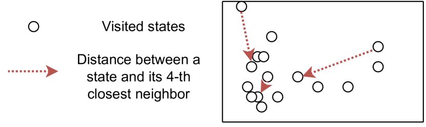
Figure 5. Illustration of the correlation between density and the fourth-nearest neighbor distance.

where $\chi(S_{b})$ is the digamma function. This approximation assumes the uniformity of states in the ball centered on a sampled state with radius $||s_{i}-nn_{k}(S_{b},s_{i})||_{2}$ (Lombardi and Pant, 2016) but its full form is unbiased with a large number of samples (Singh et al., 2003). Intuitively, it means that the entropy is proportional to the average distance between states and their neighbors. Figure 5 shows how density estimation relates to k-nearest neighbors distance. We clearly see that low-density states tend to be more distant from their nearest neighbors. Few methods (Mutti et al., 2020) provably relates to such estimations, but several approaches take advantage of the distance between state and neighbors to generate intrinsic rewards, making them related to such entropy maximization. For instance, APT (Liu and Abbeel, 2021) proposes new intrinsic rewards based on the k-nearest neighbors estimation of entropy:

(27) $$R(s,a_{t},s^{\prime})=\log(1+\frac{1}{K}\sum_{0}^{K}||f(s^{\prime})-nn_{k}(f(S_{b}),f(s^{\prime}))||_{2})$$

where $f$ is a representation function learnt with a contrastive loss based on data augmentation (Srinivas et al., 2020) and $K$ denotes the number of k-nn estimations. By looking for distant state embeddings during an unsupervised pre-training phase, they manage to considerably speed up task-learning in the DeepMind Control Suite. The representation $g$ can also derive from a random encoder (Seo et al., 2021) or a constrastive loss that ensures the euclidean proximity between consecutive states (Tao et al., 2020; Yarats et al., 2021). Alternatively, GoCu (Bougie and Ichise, 2020) achieve SOTA results on Montezuma’s revenge by learning a representation with a VAE and reward the agent based on how distant, in term of timesteps, a state is from a set of K other states.

Identifying different states.

Instead of relying on euclidean distance, one can try to learn a similarity function. EX² (Fu et al., 2017) learns a discriminator to differentiate states from each other: when the discriminator does not manage to differentiate the current state from those in the buffer, it means that the agent has not visited this state enough and it will be rewarded. States are sampled from a buffer, implying the necessity to have a large buffer. To avoid this, some methods distill recent states in a prior distribution of latent variables (Kim et al., 2019b; Klissarov et al., 2019). The intrinsic reward for a state is then the KL-divergence between a fixed diagonal Gaussian prior and the posterior of the distribution of latent variables. In this case, common latent states fit the prior while novel latents diverge from the prior.

Intra-episode novelty.

K-nearest neighbors intrinsic rewards have also been employed to improve intra-episode novelty (Stanton and Clune, 2018). It contrasts with standard exploration since the agent looks for novel states in the current episode: typically it can try to reach all states after every resets. This setting is possible when the policy depends on all its previous interactions, which is often the case when an agent evolves in a POMDP, since the agent has to be able to predict its value function even though varies widely during episodes. This way, ECO (Savinov et al., 2018) and Never give up (Badia et al., 2019) uses an episodic memory and learn to reach states that have not been visited during the current episode.

Conclusion

K-nn methods turn out to be simple to experiment, but they strongly rely on learnt dynamic-aware representations since they fully take advantage of a meaningful euclidean embedded proximity; their theoretical connection to the rigorous approximation of entropy remains most of the time unclear and the approach badly scales with an increase of the memory size. We note that simple methods can tackle the issue of finding the neighbors by partitioning together close states (Yarats et al., 2021). Overall, we observe efficient exploration and the methods easily translate to intra-episode exploration.

6.3. Conclusion

Method	Stoch	Computational cost	Montezuma’s Revenge
			Score	Steps
Direct entropy maximization
MOBE (Vezzani et al., 2019), StateEnt (Islam et al., 2019)	No	VAE	n/a	n/a
Renyi entropy (Zhang et al., 2021)	No	VAE, planning	$8100$	200M
GEM (Guo et al., 2021)	Yes	CL	n/a	n/a
SMM (Lee et al., 2019)	No	VAE, Discriminator	n/a	n/a
K-nearest neighbors approximation of entropy
EX2 (Fu et al., 2017)	No	Discriminator	n/a	n/a
(Kim et al., 2019a)			0	50M
CB (Kim et al., 2019b)	Yes	IB	$\sim 1700$	n/a
VSIMR (Klissarov et al., 2019)	No	VAE	n/a	n/a
ECO (Savinov et al., 2018)	Yes	Siamese architecture	n/a	n/a
(Bougie and Ichise, 2020)			$8032$	100M
APT (Liu and Abbeel, 2021)	n/a	CL	$0.2$	250M
RE3 (Seo et al., 2021)	Yes	ensemble of REs	$100$	5M
Proto-RL (Tao et al., 2020), Novelty (Yarats et al., 2021)	n/a	CL	n/a	n/a
NGU (Badia et al., 2019)	Yes	Inverse model, RND	$16800$	3500M
		several policies
DeepCS (Stanton and Clune, 2018)	No	RAM-based grid	$3500$	160M
GoCu (Bougie and Ichise, 2020)	n/a	VAE, predictor	$10958$	100M

• NN: Neural network. Stoch: Stochasticity. FM: Forward model. RND: (Burda et al., 2018). IB: (Alemi et al., 2016). RE: Random encoder. CL: Contrastive learning.

• They only provide the number of frames in the paper, we assume they do not use frame skip.

Table 3. Comparison between different ways to maximize novelty. Stochasticity (Stoch) indicates whether the model handles the white-noise problem. Computational cost refers to highly expensive models added to standard RL algorithm. We also report the mean score on Montezuma’s revenge (Score) and the number of timesteps executed to achieve this score (Steps). We gathered results from the original paper and in other papers than the original one. Our table does not pretend to be an exhaustive comparison of methods but tries to give an intuition on their relative advantages.

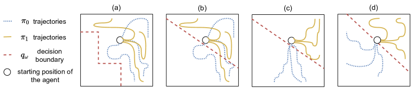
Figure 6. Illustration of the implicit learning steps of algorithms that use a fixed goal distribution. (a) Skills are not learnt yet. The discriminator randomly assigns partitions of the state space to goals. (b) The discriminator tries unsuccessfully to distinguish the skills. (c) Each skill learns to go in the area assigned to it by the discriminator. (d) Skills locally spread out by maximizing action entropy (Haarnoja et al., 2018). The discriminator successfully partitions the areas visited by each skill.

In this section, we reviewed works that maximize novelty to improve exploration with flat policies. We formalized novelty as actively discovering a representation according to the infomax principle, even though most of works only maximize the entropy of states/representations of states.

In Table 3, we give a summary of all the novelty-based methods reviewed in this section. These methods are also compared according to their performance on the sparse reward environment Montezuma’s revenge (cf. Figure 4a)), and whether they handle stochastic environments (cf. Section 5.2). We can see that these methods can better explore than surprise-based method, in particular when using intra-episode novelty mechanisms (Badia et al., 2019; Savinov et al., 2018). They can also be robust to stochasticity thanks to a specific learnt representation or the use of an ensemble of encoders (Seo et al., 2021).

Works manage to learn a representation that match the inherent structure of the environment (Tao et al., 2020). It suggests that it is most of the time enough to learn a good representation. For instance, Guo et al. (2021) and Tao et al. (2020) compute a reward based on a learnt representation, but perhaps a bad representation tends to be located in low-density areas. It would result that active representation entropy maximization correlates with state-conditional entropy minimization. We are not aware of a lot of methods that actively and explicitly maximize $I(Z;S)$ in a RL. Yet, we stress out three methods that strive to actively learn a representation of states. In CRL (Du et al., 2021) and CuRe (Aljalbout et al., 2021), the agent plays a minimax game. A module learns a representation function with a constrastive loss and the agent actively challenges the representation by looking for states with a large loss.

7. Skill learning

In our everyday life, nobody has to think about having to move his arms’ muscles to grasp an object. A command to take the object is just issued. This can be done because an acquired skill can be effortlessly reused.

Skill abstraction denotes the ability of an agent to learn a representation of diverse skills. We formalize skill abstraction as maximizing the mutual information between the goal $g\in G$ and some of the rest of the contextual states $f(\tau)\in u(\mathcal{T})$, denoted as $I(G;u(\mathcal{T}))$ where $\tau\in\mathcal{T}$ is a trajectory and $f$ a function that extracts a subpart of the trajectory (last state for example). The definition of $u$ depends on the wanted semantic meaning of a skill. Let $s_{0}$ refers to the state at which the skill started and $s$ a random state from the trajectory, we highlight two settings based on the literature:

• $u(\mathcal{T})=S$, the agent learns skills that target a particular state of the environment (Eysenbach et al., 2018).

• $u(\mathcal{T})=\mathcal{T}$, the agent learns skills that follow a particular trajectory. This way, two different skills can end in the same state if they cross different areas (Co-Reyes et al., 2018).

Most of works maximize $I(G;S)$ so that, unless stated otherwise, we refer to this objective. In the following, we will study the different ways to maximize $I(G;S)$ which can be written under its reversed form $I(S;G)=H(G)-H(G|S)$ or forward form $I(G;S)=H(S)-H(S|G)$ (Campos et al., 2020). In particular, we emphasize that:

(28a) $$-H(G|S) =\sum_{g\in G,s\in S}p(g,s)\log p(g|s)$$

(28b) $$=\mathbb{E}_{\begin{subarray}{c}g\sim p(g)\\ s\sim\pi^{g}\end{subarray}}\log p(g|s)$$

where, to simplify, $p(g)$ is the current distribution of goals (approximated with a buffer) and $s\sim\pi^{g}$ denotes the distribution of states that results from the policy that achieves $g$. Note that $p(g,s)=p(s|g)p(g)$.

In this section, we first focus on methods that assume they can learn all skills induced by a given goal space/goal distribution and they assign parts of trajectories to every goal. The second set of methods directly derives the goal space from visited states, so that there are two different challenges that we treat separately: the agent has to learn to reach a selected goal and it must maximize the diversity of goals it learns to reach. We make this choice of decomposition because some contributions focus on only one part of the objective function.

7.1. Fixing the goal distribution

The first approach assumes the goal space is arbitrarily provided except for the semantic meaning of a goal. In this setting, the agent samples goals uniformly from $G$, ensuring that $H(G)$ is maximal, and it progressively assigns all possible goals to a part of the state space. To do this assignment, the agent maximizes the reward provided by Equation 28b:

(29) $$R(g,s,a,s^{\prime})=-\log q_{\omega}(g|s^{\prime})$$

where $q_{\omega}(g|s^{\prime})$ represents a learnt discriminator (often a neural network) that approximates $p(g|s^{\prime})$.

At first, we focus on discrete number of skills, where $p(g)$ represents a uniform categorical distribution. Figure 6 sums up the learning process with two discrete skills: 1- skills and discriminator $q_{\omega}$ are randomly initialized; 2- the discriminator tries to differentiate the skills with states $s$ from its trajectories, in order to approximate $p(g|s)$; 3- skills are rewarded with Equation 29 in order to make them go in the area assigned to it by the discriminator; 4- finally, skills are clearly distinguishable and target different parts of the state space. SNN4HRL (Florensa et al., 2017) and DIAYN (Eysenbach et al., 2018) implement this procedure by approximating $g$ with, respectively, a partition-based normalized count and a neural network. VALOR (Achiam et al., 2018) also uses a neural network, but discriminate discrete trajectories. In this setting, the agent executes one skill per episode.

HIDIO (Zhang et al., 2020b) sequentially executes skills, yet that is not clear how they manage to avoid forgetting previously learnt skills. Maximizing $I(G;S|S_{0})$ like VIC (Gregor et al., 2016) or $I(G;S_{0}|S)$ with R-VIC (Baumli et al., 2021) makes it hard to use a uniform (for instance) $H(G|S_{0})$, because every skill may not be executable everywhere in the state space. Therefore, they also maximize the entropy term with another reward bonus similar to $\log p(g|s_{0})$. They learn discriminable skills, but still struggle to combine them on complex benchmarks (Baumli et al., 2021). Keeping $p(g)$ uniform, DADS (Sharma et al., 2020) maximizes the forward form of mutual information $I(S;G|S_{0})=H(S|S_{0})-H(S|G,S_{0})$ by approximating $p(s|s_{0})$ and $p(s|s_{0},g)$. This method makes possible to plan over skills and can combine several locomotion skills. However this requires several conditional probability density estimation on the ground state space, which may badly scale on higher-dimensional environments.

These methods tend to stay close from their starting point (Campos et al., 2020) and do not learn skills that cover the whole state space. In fact, it is easier for the discriminator to overfit over a small area than to make a policy go in a novel area, this results with a lot of policies that target a restricted part of the state space (Choi et al., 2021). Accessing the whole set of true possible states and deriving the set of goals by encoding states can considerably improve the coverage of skills (Campos et al., 2020).

Approaches for a better coverage of states.

Heterogeneous methods address the problem of overfitting of the discriminator. The naive way can be to regularize the learning process of the discriminator. ELSIM (Aubret et al., 2020) takes advantages of L2 regularization and progressively expand the goal space $G$ to cover larger areas of the state space and Choi et al. (2021) propose to use spectral normalization (Miyato et al., 2018). More consistent dynamic-aware methods may further improve regularization; however it remains hard to scale the methods to a large number of skills which are necessary to scale to a large environment. In above-mentioned methods, the number of skills greatly increases (Achiam et al., 2018; Aubret et al., 2020) and the discrete skill embedding does not provide information about proximity of skills. Therefore learning a continuous embedding may be more efficient.

Continuous embedding.

The prior uniform distribution $p(g)$ is far more difficult to set in a continuous embedding. One can introduce the continuous DIAYN (Choi et al., 2021; Zhang et al., 2020b) with a prior $p(G)=\mathcal{N}(0^{d},I)$ where $d$ is the number of dimensions, or the continuous DADS with a uniform distribution over $[-1;1]$ (Sharma et al., 2020), yet it remains unclear how the skills could adapt to complex environments, where the prior does not globally fit the inherent structure of the environment (e.g a disc-shaped environment). VISR (Hansen et al., 2020) seems to, at least partially, overcome this issue with a long unsupervised training phase and successor features. They uniformly sample goals on the unit-sphere and computes the reward as a dot product between unit-normed goal vectors and successor features $\log q_{\omega}(g|s)=\phi_{successor}(s)^{T}g$.

Conclusion.

This set of methods manages to learn discrete skills that can be combined, yet, despite regularization, discrete skills struggle to cover a very large state space (Aubret et al., 2020). Successful adaptations to scale it up to large states spaces currently rely on the relevance of successor features. In the next two sections, we study how to maximize the mutual information by assuming the goal space derives from the state space.

7.2. Achieving a state-goal

In this section, we review how current methods maximize the goal achievement part of the objective of the agent, $-H(S_{g}|S)$ where $S_{g}$ refers to the goal-relative embedding of states. We temporally set aside $H(S_{g})$ and we will come back to this in the next subsection, Section 7.3, mainly because the two issues are tackled separately in the literature.

Obviously, maximizing $-H(S_{g}|S)$ can be written:

(30) $$-H(S_{g}|S) =\sum_{S_{g},S}p(s_{g},s)\log p(s_{g}|s)=\mathbb{E}_{\begin{subarray}{c}s_{g}\sim p(s)\\ s\sim\pi^{g}\end{subarray}}\log p(s_{g}|s)$$

where, to simplify, $p(s)$ is the current distribution of states (approximated with a buffer) and $s\sim\pi^{g}$ denotes the distribution of states that results from the policy that achieves $g$. If $\log p(s_{g}|s^{\prime})$ is modelled as an unparameterized Gaussian with a unit-diagonal co-variance matrix, we have $\log p(s_{g}|s^{\prime})\propto-||s_{g}-s^{\prime}||_{2}^{2}+Const$ so that we can reward an agent according to:

(31) $$R(s_{g},s,a,s^{\prime})=-||s_{g}-s^{\prime}||_{2}^{2}.$$

It means that if the goal is a state, the agent must minimize the distance between its state and the goal state. To achieve this, it can take advantage of a goal-conditioned policy $\pi^{s_{g}}(s)$.

Ground state space.

This way, Hierarchical Actor-Critic (HAC) (Levy et al., 2019) directly uses the state space as a goal space to learn three levels of option (the options from the second level are selected to fulfill the chosen option from the third level). A reward is given when the distance between states and goals (the same distance as in Equation 31) is below a threshold and they take advantage of HER to avoid to directly use the threshold. Similar reward functions can be found in Pitis et al. (2020) and Zhao et al. (2019). Related to these works, HIRO (Nachum et al., 2018) uses as a goal the difference between the initial state and the state at the end of the option $f(\mathcal{T})=S_{f}-S_{0}$.

This approach is relatively simple and does not require extra neural networks. However, there are two problems in using the state space in the reward function. Firstly, a distance (like L2) makes little sense in a very large space like images composed of pixels. Secondly, it is difficult to make a manager policy learn on a too large action space. Typically, an algorithm having as goals images can imply an action space of $84\times 84\times 3$ dimensions for a goal-selection policy (in the case of an image with standard shape). Such a wide space is currently intractable, so these algorithms can only work on low-dimensional state spaces.

Learning a representation of goals.

To tackle this issue, an agent can learn low-dimensional embedding of space $\phi_{e}$ and maximize the reward of Equation 32 using a goal-conditioned policy $\pi^{f(s_{g})}(s)$:

(32) $$R(s_{g},s,a,s^{\prime})=-||f(s_{g})-f(s^{\prime})||_{2}^{2}.$$

Similarly to Equation 31, this amounts to maximize $-H(f(S_{g})|f(S))$. RIG (Nair et al., 2018) proposes to build the feature space independently with a variational auto-encoder (VAE); but this approach can be very sensitive to distractors (i.e. useless features for the task or goal, inside states) and does not allow to correctly weight features. Similar approaches also encode part of trajectories (Kim et al., 2021; Co-Reyes et al., 2018) for similar mutual information objectives. SFA-GWR-HRL (Zhou et al., 2019) uses unsupervised methods like the algorithms of slow features analysis (Wiskott and Sejnowski, 2002) and growing when required (Marsland et al., 2002) to build a topological map. A hierarchical agent then uses nodes of the map, representing positions in the world, as a goal space. However the authors do not compare their contribution to previous approaches.

Other approaches learn a state embedding that captures the proximity of states with contrastive losses. For instance, DISCERN learns the representation function by maximizing the mutual information between the last state representation and the state-goal representation. Similarly to works in Section 7.1, the fluctuations around the objective allow to bring states around $s_{g}$ closer to it in the representation. More explicitly, the representation of NOR (Nachum et al., 2019a) maximizes $I(f(S_{t+k});f(S_{t}),A_{t:t+k})$ and the one of LESSON (Li et al., 2021b) maximizes $I(f(S_{t+1});f(S_{t}))$; LESSON and NOR target a change in the representation and manage to navigate in a high-dimensional maze while learning the intrinsic Euclidean structure of the mazes (cf. Table 4). Their skills can be reused on several environments. However, experiments are made in 2-dimensional embedding spaces and it remains unclear how relevant may be goals as state changes in an embedding space with higher dimensions. The more the number of dimensions increase, the more difficult it will be to distinguish possible skills from impossible skills in a state. In addition, they need dense extrinsic rewards to learn to select the skills to execute. Thus, they generate tasks with binary rewards at a location uniformly distributed in the environment such that the agent learn to achieve the tasks from the simplest to the hardest. This progressive learning generates a curriculum, helping to achieve the hardest task.

Conclusion.

To sum up, representation learning methods allows to learn state-based skills over complex state spaces. Learning this representation function combined with the use of the euclidean distance as reward function amounts to learn a particular form of reward function in addition for providing pre-computed features to the goal-conditioned policy. As highlighted by Table 4, learnt representations allow to scale the approaches to more complex goal spaces. In the next paragraph, we study how to maximize $H(S)$ so that to make sure learnt skills target different areas of the state space. As highlighted by Table 4, it will make possible to reach very distant goals without being assisted by a curriculum of tasks.

7.3. Proposing diverse state-goals

To make sure the agent maximizes the mutual information between its goals and all visited states, it must sample a diverse set of goal-states. In other words, it has to maximize $H(S_{g})$ but through goal selection rather than with an intrinsic bonus as in Section 6. Similarly to works on novelty (cf. Section 6), such entropy maximization along with skill acquisition (cf. Section 7.2) tackles the exploration challenge, but without facing catastrophic forgetting (cf. Section 8.1) since the agent does not forget its skills.

A naive approach would be to generate random values in the goal space, but this faces a considerable problem: the set of achievable goals is often a very small subset of the entire goal space. To tackle this, a first approach can be to explicitly learn to differentiate these two sets of goals (Florensa et al., 2018; Racaniere et al., 2019), using for example a Generative Adversarial Networks (GAN) (Florensa et al., 2018; Goodfellow et al., 2014), but it is ineffective in complex environments (Pong et al., 2020). Other works obtain good results on imagining new goals, but using a compoundable goal space, given (Colas et al., 2019) or learnt with a dataset (Khazatsky et al., 2021); results show it may be a strong candidate for object-based representations. In contrast, in a more general case, an agent can simply set a previously met state as a goal, this way, it ensures that goals are reachable, since they have already been achieved. In the rest of this section, we focus on this set of methods.

In RIG (Nair et al., 2018), the agent randomly samples states as goals from its buffer, but it does not increase the diversity of states, and thus, the diversity of learnt skills. Pong et al. (2020) showed theoretically and empirically that, by sampling goals following a $\alpha$-more uniform distribution over the support of visited states than the ”achieved” distribution, the distribution of states of the agent can converge to the uniform distribution. Intuitively, the agent just samples more often low-density goals as illustrated it in Figure 7. There are several ways to increase the importance of low-density goal-states that we introduce in the following.

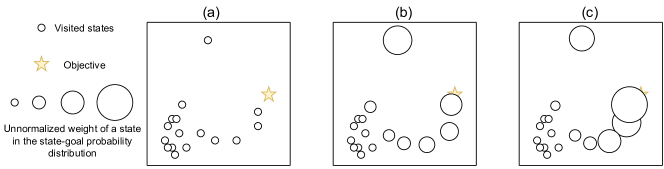
Figure 7. Illustration of the reweighting process. (a) probability of visited states to be selected as goals before reweighting; (b) probability of visited states to be selected as goals after density reweighting; (c) probability of visited states to be selected as goals after density/reward reweighting. This figure completes and simplifies the figure of Pong et al. (2020).

Density estimation in the ground state space.

DISCERN (Warde-Farley et al., 2019) proposes to sample uniformly over the support of visited stated with a simple procedure. Every time the agent wants to add an observation to its buffer, it randomly samples an other observation from its buffer and only keeps the one that is the farthest to all other states of the buffer. This way, it progressively builds an uniform distribution of states inside its buffer. However, it uses the euclidean distance to compare images, which may not be relevant. Other approaches select the state that has the lower density (OMEGA) (Pitis et al., 2020) according to a kernel density estimation or use the rank of state-densities (Zhao and Tresp, 2019) estimated with a Variational Gaussian Mixture Model (Blei and Jordan, 2006). In contrast with them, Skew-fit (Pong et al., 2020) provides more flexibility on how uniform one want its distribution of states. Skew-fit extends RIG and learns a parameterized generative model $q_{\rho}(S)\approx p(S)$ and skews the generative model (VAE) with the ratio:

(33) $$q_{\rho}(s)^{\alpha_{skew}}$$

where $\alpha_{skew}<0$ determines the speed of uniformisation. This way it gives more importance to low-density states. Then it weights all visited states according to the density approximated by the generative model at the beginning of each epoch, which is made of a predefined number of timesteps. Skew-fit manages to explore image-based environments very efficiently. As highlighted in (Aubret et al., 2021), this ratio applied on a discrete number of skills, amount to rewards a Boltzmann goal-selection policy with:

(34) $$R(s_{g})=(1+\alpha_{skew})\log p(s_{g}).$$

Density reweighting by partitioning the embedding space.

With a different objective, GRIMGREP (Kovač et al., 2020) partitions the VAE embedding of Skew-fit with a Gaussian Mixture Model (Rasmussen et al., 1999) to estimate the learning progress of each partition and avoid distractors. The density weighting can also operate in a learnt embedding. HESS (Li et al., 2021a) partitions the embedding space of LESSON and rewards with a variant of a count-based bonus (see Section 5). It improves exploration in a two-dimensional latent embedding but the size of partitions may not scale well if the agent considers more latent dimensions. In contrast, DisTop (Aubret et al., 2021) dynamically clusters a dynamic-aware embedding space using a variant of a Growing When Required (Marsland et al., 2002); they estimate the density of state according to how much its partition contains states and skew the distribution of sampled similarly to Skew-fit. HESS and DisTop demonstrate their ability to explore and navigate with an ant inside complex mazes without extrinsic rewards. As shown in (Aubret et al., 2021) (illustration in Figure 7c), it is also possible to use extrinsic rewards to weight the distribution of sampled state-goals.

Conclusion.

Entropy maximization methods improves over standard skill learning methods by learning to reach as many states as possible. We expect further works to show the ability to scale to even more complex environments, with higher-dimensional latent structure. For example, learning compositional representations ( modeling disentangled objects and relations) remains hard: SOTA methods only manipulate few objects (Pong et al., 2020).

7.4. Conclusion

Fixing the goal distribution
SNN4HRL (Florensa et al., 2017), DIAYN (Eysenbach et al., 2018), VALOR (Achiam et al., 2018)
HIDIO (Zhang et al., 2020b), R-VIC (Baumli et al., 2021), VIC (Gregor et al., 2016)
DADS (Sharma et al., 2020), continuous DIAYN (Choi et al., 2021), ELSIM (Aubret et al., 2020)
VISR (Hansen et al., 2020)
Methods	Scale	Goal space	Curriculum	Score	Steps
Achieving a state-goal
HAC (Levy et al., 2019)	n/a	n/a	n/a	n/a	n/a
HIRO (Nachum et al., 2018)	4x	(x,y)	Yes	$\sim 0.8$	4M
RIG (Nair et al., 2018)	n/a	n/a	n/a	n/a	n/a
SeCTAR (Co-Reyes et al., 2018)	n/a	n/a	n/a	n/a	n/a
IBOL (Kim et al., 2021)	n/a	n/a	n/a	n/a	n/a
SFA-GWR-HRL (Zhou et al., 2019)	n/a	n/a	n/a	n/a	n/a
NOR (Nachum et al., 2019a)	4x	T-V + P	Yes	$\sim 0.7$	10M
(Li et al., 2021b)	4x	T-V + P	Yes	$\sim 0.4$	4M
LESSON (Li et al., 2021b)	4x	T-V + P	Yes	$\sim 0.6$	4M
Proposing diverse state-goals
Goal GAN (Florensa et al., 2018)	1x	(x,y)	No	Coverage $0.71\%$	n/a
(Pong et al., 2020)	n/a (1̃6x)	(x,y)	No	All goals distance $\sim 7$	7M
FVC (Racaniere et al., 2019)	n/a	n/a	n/a	n/a	n/a
Skew-fit (Pong et al., 2020)	n/a (1̃6x)	(x,y)	No	All goals distance $\sim 1.5$	7M
DisTop (Aubret et al., 2021)	4x	T-V	No	$\sim 1$	2M
DISCERN (Warde-Farley et al., 2019)	n/a	n/a	n/a	n/a	n/a
OMEGA (Pitis et al., 2020)	4x	(x,y)	No	$\sim 1$	4.5M
CDP (Zhao and Tresp, 2019)	n/a	n/a	n/a	n/a	n/a
(Pong et al., 2020)	n/a (1̃6x)	(x,y)	No	All goals distance $\sim 7.5$	7M
GRIMGREP (Kovač et al., 2020)	n/a	n/a	n/a	n/a	n/a
HESS (Li et al., 2021a)	4x	T-V + P	No	success rate $\sim 1$	6M

Table 4. Summary of papers that learn skills through mutual information maximization. We selected the Ant Maze environment to compare methods since this is the most commonly used environment. We did not find a common test setting allowing for a fair comparison of methods in ”Fixing the goal distribution”. The scale refers to the size of the used maze. Goal space refers to the a priori state space used to compute goals, from the less complex to the more complex: (x,y); 75-dimensional top-view of the maze (T-V); top-view + proprioceptive state (T-V + P). Curriculum refers to whether the authors use different goal locations during training, creating an implicit curriculum that makes easier learning to reach distant goals from the starting position. The score, unless stated otherwise, refers to the success rate in reaching the farthest goal.

We found two main ways to discover skills. The first one provides a goal space and assigns goals to areas of the state space. There are empirical evidences emphasizing that it struggles to learn and sequentially executes skills that target different areas of the state space. The second method derives the goal space from the state space with a representation learning method and over-weights the sampling of low-density visited areas. This set of works showed the ability to hierarchically navigate in simple environments using moderately morphologically complex agents.

In Table 4, we synthesize the methods presented in this section. We also compare skill learning methods according to their performance on the widely used hierarchical task Ant maze (cf. Figure 4b)), and whether they need a hand-made goal space (x,y) or an implicit curriculum of objectives. We can make two major observations: 1- methods that do not propose diverse goal-states require an implicit curriculum to learn the Ant-Maze task (Nachum et al., 2018; Li et al., 2021b) (Curriculum column); 2- contrastive representations seem crucial to avoid using a hand-defined goal space like the (x,y) coordinated (Goal space column) (Nachum et al., 2019a; Li et al., 2021a). For methods in the ”fixing the goal distribution”, we did not find a representative and widely used evaluation protocol/environment among works. However, as an example, several qualitative analysis emphasize the diversity of behaviors that can be learnt by the ant displayed in Figure 4c) (Sharma et al., 2020; Eysenbach et al., 2018).

8. Outlooks of the domain

In this section, we take a step back and thoroughly analyze the results of our overall review. We first study the exploration process of flat intrinsic motivation in comparison with hierarchical intrinsic motivations in Section 8.1; then, this will motivate our focus on the challenges induced by learning a deep hierarchy of skills in Section 8.2. Finally, in Section 8.3, we discuss how flat and hierarchical intrinsic motivations can and should cohabit in such hierarchy.

8.1. Long-term exploration, detachment and derailment

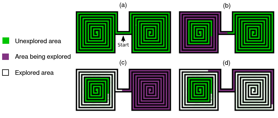
Figure 8. Illustration of the detachment issue. Image extracted from Ecoffet et al. (2019). Green color represents intrinsically rewarding areas, white color represents no-rewards areas and purples areas are currently being explored. (a) The agent has not explored the environment yet. (b) It discovers the rewarding area at the left of its starting position and explores it. (c) It consumed close intrinsic rewards on the left part, thus it prefers gathering the right-part intrinsic rewards. (d) Due to catastrophic forgetting, it forgot how to reach the intrinsically rewarding area on the left.

The most challenging used benchmarks in flat intrinsic motivations (surprise and novelty) are DMLab and Montezuma’s revenge, yet very sparse reward games such as Pitfall! are not currently addressed and should be investigated. In Pitfall!, the first reward is reached only after multiple rooms where it requires specific action sequences to go through each room. State of the art on IM methods (Ostrovski et al., 2017) achieve 0 mean reward in this game. At the opposite, imitation RL methods (Aytar et al., 2018; Hester et al., 2018) are insensitive to such a specific reward, and thus, exceed IM methods with a mean reward of 37232 on Montezuma’s revenge and 54912 on Pitfall!. Even though these methods use expert knowledge, this performance gap exhibits their resilience to long-term rewards. Compared with flat intrinsic reward methods, which do not exceed a 10000 score on Montezuma’s revenge (Burda et al., 2018) and hardly achieve a score on Pitfall! (Ostrovski et al., 2017), it shows that flat IMs is still far from solving the overall problem of exploration.

Furthermore, we want to emphasize that the challenge is harder when the intrinsic reward itself is sparse (Burda et al., 2018). In Montezuma’s revenge, it is about avoiding to use a key too quickly in order to be able to use it later. In every day life, it can be about avoiding to spend money too quickly. In fact, it looks like there is an exploration issue in the intrinsic reward function. Intrinsic reward can guide the exploration at the condition that the agent finds this intrinsic reward. There may be two reasons causing the intrinsic reward to be sparse:

1. The first comes from partial observability, with which most models are incompatible. Typically, if an agent has to push a button and can only see the effect of this pushing after a long sequence of actions, density models and predictive models may not provide meaningfull intrinsic rewards. There would be a too large distance between the event ”push a button” and the intrinsic reward.

2. Figure 8 illustrates the second issue, called detachment (Ecoffet et al., 2019, 2021). It results from a distant intrinsic reward coupled with catastrophic forgetting. Simply stated, the RL agent can forget the presence of an intrinsic reward in a distant area: this is hard to maintain the correct Q-value that derives from a distant currently unvisited rewarding area. This is emphasized in on-policy settings.

Pursuing such distant intrinsic reward may be even harder due to the possible derailment issue (Ecoffet et al., 2019, 2021). Essentially, an agent may struggle to execute a long sequence of specific actions needed to reach a distant rewarding area because the local stochasticity incites local dithering all along the sequence. Detachment motivates the need for a hierarchical exploration (Ecoffet et al., 2021) and derailment motivates frontier-based exploration (Bharadhwaj et al., 2020), which consists in deterministically reaching the area to explore before starting exploration.

8.2. Deeper hierarchy of skills

According to Brooks (1991), everything is grounded in primitive sensor motor patterns of activation. This everything may refer to the structure of the world and agent affordances. Capturing this knowledge amounts to form concept representations and reusable skills (Weng et al., 2001), use it as a basis for new skills (Prince et al., 2005), explore the environment to find new interesting skills, autonomously self-generate goals in accordance with the level and morphology of the agent.

Most works presented in Section 7 abstract actions on a restricted number of hierarchies (generally one hierarchy). This is necessary to well-understand the mechanism of abstraction, but we want to argue that imposing deeper hierarchies could considerably enhance the semantic comprehension of the environment of an agent. Organisms are often assumed to deal with composition of behaviors, which in turn serve as building block for more complex behaviors (Flash and Hochner, 2005). This way, using a limited vocabulary of skills makes easier avoiding the curse of dimensionality associated to the redundancy of a whole set of ground behaviors.

Our surveyed works (Nachum et al., 2019a; Aubret et al., 2021; Li et al., 2021b; Guo et al., 2021; Ermolov and Sebe, 2020) already propose to learn the representations using the slowness principle (Wiskott and Sejnowski, 2002) which assumes temporally close states should be similarly represented. By configuring the time-extension of the representation, one may focus on different semantic parts of the state space. This can be seen in Section 3.2: 1- the agent can learn a very low level representation that provides skills that can manipulate torques of a creature (Aubret et al., 2021); 2- skills can also orientate an agent in a maze by extracting (x,y) coordinates from a complex state representation (Li et al., 2021a). While they do not try to combine and learn several representations at the same time, further works could consider separate different parts of states (e.g. agent positions and object positions (Zhao et al., 2021)) or learning these representations at different time scales. In practice, data-augmentation methods already allow to learn object-oriented representations (Mitrovic et al., 2020; Grill et al., 2020; Mussa-Ivaldi and Solla, 2004). Most augmentations could also be derived with contrast over time by considering, for instance, an embodied agent moving its eyes/head (crops), turning its head (rotation), controlling vergence (blur) or, without interventions, color and brightness changes (Chen et al., 2020). Overall, it stresses out the potential of time-contrastive representations for disentangling the whole state space and providing semantically different skills; new works in this area may unlock new kind of skills.

Skill focus. In a developmental process, multi-level hierarchical RL questions the ability of the agent to learn all policies of the hierarchy simultaneously. This obviously relates to the ability of organisms to continually learn throughout their lifetime; but in more practical way, it may allow to focus the learning process of skills that are interesting for higher-level skills. This focus avoids learning everything in the environment (Aubret et al., 2021), which is hard and obviously not done by biological organisms. For instance, most persons can not do a somersault.

Critical periods and lifelong learning. Considering a goal representation that changes over time introduces new issues for the agent. In this case, the goal-conditioned policy may be perturbed by the changes of inputs and may no longer be able to reach the goal (Li et al., 2021a). Current methods consider 1- developmental periods (unsupervised pre-training (Metzen and Kirchner, 2013)); 2- to modify the representation every k-steps epochs (Pong et al., 2020); 3- to impose slowly changes of the representation (Li et al., 2021a). Further works may thoroughly investigate the relation and transitions between these methods since they can relate to the concept of critical periods (Hensch, 2004; Konczak, 2004). Critical periods assume that the brain is more plastic at some periods of development in order to acquire specific knowledge. Despite this mechanism, the brain slowly keeps learning throughout the lifetime. In the hierarchy of skills, the introduction of a new level may first result in a quick/plastic learning process, followed by slower changes.

8.3. The role of flat intrinsic motivations

In Section 8.1, we essentially criticized the limited role that flat intrinsic motivation like surprise or novelty can play in favor of exploration and we hypothesized in Section 8.2 that deeper hierarchies could make emerge an understanding of more complex affordances. Then, what could be the roles of surprise and novelty ?

Novelty. We saw in Section 6 that novelty seeking behaviors allow to learn a correct representation of the whole environment; this can be a basis for learning diverse skills. While some methods consider a goal as a state and manage to avoid using novelty bonuses (Pong et al., 2020), this is harder to do when skills have a different semantic (like a change in the state space). Nachum et al. (2019a) provide a meaningful example of this: the agent acts to simultaneously discover a representation of the environment and achieve upper-level goals.

Surprise. We leave aside the interest of surprise for learning a forward model that could be used for planning (Hafner et al., 2019b) and rather focus on the learning process. Surprise amounts to look for the learning progress of forward models so that, in a hierarchy of skills, it quantifies whether skills can currently be better learnt or not. This links surprise to curriculum learning (Bengio et al., 2009), i.e can we find a natural order to efficiently learn skills ? For example, assuming an agent want to learn to reach state-goal in a maze, it would be smarter to learn to start learning skills that target goals close to its starting position and to progressively extend its goal selection while learning other skills. Several strategies have been proposed to smartly hierarchically select goals (Colas et al., 2019; Linke et al., 2020), yet it often does not consider intrinsic skills (Colas et al., 2019).

To sum up, we propose that the role of surprise and novelty may rather be to support the learning of skills. Novelty seeking helps to learn the representation required by the skill learning module and surprise speeds up the maximization of the skill learning objective. They may interact as a loop: first, the agent learns a new representation, then it evaluates surprise to select which skill to improve and the skill learning process starts. Considering this, it would result several surprises and novelties: an agent can experiment a novel or surprise interaction for a level of decision (injure the toy while walking), yet it does not mean other levels would be surprised (it is still on the same road). This emphasizes the multi-dimensionality and relativity of the notion of surprise ou novelty (Berlyne, 1960), only a part of the incoming stimuli may arouse the agent.

9. Conclusion

In this survey, we have presented the current challenges faced by DRL: namely 1- learning with sparse rewards through exploration; 2- building a hierarchy of skills in order to make easier credit assignment, exploration with sparse rewards and transfer learning.

We identified several types of IM to tackle these issues, that we classified into three categories based on a maximized information theoretic objective, which are surprise, novelty and skill learning. Surprise and novelty based intrinsic motivations implicitly improve flat exploration while skill learning allows to create a hierarchy of reusable skills that also improve exploration.

Surprise results from maximizing the mutual information between the true model parameters and the next state, knowing the previous state, the action and the history of interactions. We have shown that it can be maximized through three set of works: information gain over predictive models, over density models or prediction errors/learning progress. In practice, we found that the information gain over density model is ill-defined for purely stochastic areas and that the determinism assumption underpinning prediction error methods complicates their application. Good approximations of surprise are notably useful to allow exploration in stochastic environments. Next challenges may be to make good approximations of surprise tractable.

Novelty seeking can be assimilated to learning a representation of the environment, through the maximization of mutual information between states and their representation. The most important term to actively maximize looks to be the entropy of state or representation, which can be approximated in two ways: 1- one can reward according to the parametric density of its next state, but it is complicated to estimate; 2- one can also reward an agent according to the distance between a state and currently already visited states, making the approach tractable in particular when the agent learns a dynamic-aware representation. We found these methods to achieve state-of-the-art performance on the hard exploration task Montezuma’s Revenge. We expect future works to benefit from directly looking for good representations rather than uniformity of states.

Finally, using skill learning objective that amount to maximize the mutual information between a goal and a part of trajectories of the corresponding skill, an agent can learn hierarchies of temporally-extended skills. Skills can be directly learnt by attributing part of a fixed goal space to areas, but it remains to clarify how well goals can be embedded in a continuous way and whether approaches may be robust when skills are sequentially executed. The second approach derives the goals space from the state space, often through a time-contrastive loss, and expand the skill set by targeting low-density areas. These methods manage to explore an environment while being able to return to previously visited areas. It remains to be demonstrated how one could create larger hierarchies of skills.

The three objectives are compatible and we have discussed how they could interact to provide a robust exploration with respect to the detachment issue, along with reusable hierarchical skills, a quick and focused skill acquisition and multi-semantic representations.

Appendix A Notations

$\propto$	Proportional to
$x\sim p(\cdot)$	$x\sim p(x)$
$||x||_{2}$	Euclidian norm of $x$
$t$	timestep
$Const$	arbitrary constant
$A$	set of possible actions
$S$	set of possible states
$a\in A$	action
$s\in S$	state
$s_{0}\in S$	first state of a trajectory
$s_{f}\in S$	final state of a trajectory
$s^{\prime}\in S$	state following a tuple $(s,a)$
$h$	history of interactions $(s_{0},a_{0},s_{1},\dots)$
$\hat{s}$	predicted states
$g\in G$	goal
$s_{g}\in S$	state used as a goal
$S_{b}$	set of states contained in $b$
$\tau\in\mathcal{T}$	trajectory
$u(\tau)$	function that extracts parts of the trajectory $\tau$
$R(s,a,s^{\prime})$	reward function
$d^{\pi}_{t}(s)$	t-steps state distribution
$d^{\pi}_{0:T}(S)$	stationary state-visitation distribution of $\pi$ over a horizon T
	$\frac{1}{T}\sum_{t=1}^{T}d^{\pi}_{t}(S))$
$f$	representation function
$z$	compressed latent variable, $z=f(s)$
$\rho\in\mathrm{P}$	density model
$\phi\in\Phi$	forward model
$\phi_{T}\in\Phi_{T}$	true forward model
$q_{\omega}$	parameterized discriminator
$\pi$	policy
$\pi^{g}$	policy conditioned on a goal $g$
$nn_{k}(S,s^{\prime})$	k-th closest state to $s^{\prime}$ in $S$
$D_{KL}(p(x)||p^{\prime}(x))$	Kullback–Leibler divergence
	$\mathbb{E}_{x\sim p(\cdot)}\log\frac{p(x)}{p^{\prime}(x)}$
$H(X)$	$-\int_{X}p(x)\log p(x)$
$H(X|S)$	$-\int_{S}p(s)\int_{X}p(x|s)\log p(x|s)dxds$
$I(X;Y)$	$H(X)-H(X|Y)$
$I(X;Y|S)$	$H(X|S)-H(X|Y,S)$
$IG(h,A,S^{\prime},S,\Phi)$	Information gain
	$I(S^{\prime};\Phi|h,A,S)$

Table 5. Notations used in the paper.

References

- (1)
- Achiam et al. (2018) Joshua Achiam, Harrison Edwards, Dario Amodei, and Pieter Abbeel. 2018. Variational option discovery algorithms. arXiv preprint arXiv:1807.10299 (2018).
- Achiam and Sastry (2017) Joshua Achiam and Shankar Sastry. 2017. Surprise-based intrinsic motivation for deep reinforcement learning. arXiv preprint arXiv:1703.01732 (2017).
- Alemi et al. (2016) Alexander A Alemi, Ian Fischer, Joshua V Dillon, and Kevin Murphy. 2016. Deep variational information bottleneck. arXiv preprint arXiv:1612.00410 (2016).
- Aljalbout et al. (2021) Elie Aljalbout, Maximilian Ulmer, and Rudolph Triebel. 2021. Seeking Visual Discomfort: Curiosity-driven Representations for Reinforcement Learning. arXiv preprint arXiv:2110.00784 (2021).
- Almeida (2003) Luís B Almeida. 2003. MISEP–linear and nonlinear ICA based on mutual information. Journal of Machine Learning Research 4, Dec (2003), 1297–1318.
- Amin et al. (2021) Susan Amin, Maziar Gomrokchi, Harsh Satija, Herke van Hoof, and Doina Precup. 2021. A Survey of Exploration Methods in Reinforcement Learning. arXiv preprint arXiv:2109.00157 (2021).
- Amodei et al. (2016) Dario Amodei, Chris Olah, Jacob Steinhardt, Paul Christiano, John Schulman, and Dan Mané. 2016. Concrete problems in AI safety. arXiv preprint arXiv:1606.06565 (2016).
- Andrychowicz et al. (2017) Marcin Andrychowicz, Filip Wolski, Alex Ray, Jonas Schneider, Rachel Fong, Peter Welinder, Bob McGrew, Josh Tobin, OpenAI Pieter Abbeel, and Wojciech Zaremba. 2017. Hindsight experience replay. In Advances in Neural Information Processing Systems. 5048–5058.
- Aubret et al. (2021) Arthur Aubret, Salima Hassas, et al. 2021. DisTop: Discovering a Topological representation to learn diverse and rewarding skills. arXiv preprint arXiv:2106.03853 (2021).
- Aubret et al. (2020) Arthur Aubret, Laëtitia Matignon, and Salima Hassas. 2020. ELSIM: End-to-end learning of reusable skills through intrinsic motivation. In European Conference on Machine Learning and Principles and Practice of Knowledge Discovery in Databases (ECML-PKDD).
- Audibert et al. (2007) Jean-Yves Audibert, Rémi Munos, and Csaba Szepesvári. 2007. Tuning bandit algorithms in stochastic environments. In International conference on algorithmic learning theory. Springer, 150–165.
- Aytar et al. (2018) Yusuf Aytar, Tobias Pfaff, David Budden, Thomas Paine, Ziyu Wang, and Nando de Freitas. 2018. Playing hard exploration games by watching youtube. In Advances in Neural Information Processing Systems. 2930–2941.
- Azar et al. (2019) Mohammad Gheshlaghi Azar, Bilal Piot, Bernardo Avila Pires, Jean-Bastien Grill, Florent Altché, and Rémi Munos. 2019. World discovery models. arXiv preprint arXiv:1902.07685 (2019).
- Bacon et al. (2017) Pierre-Luc Bacon, Jean Harb, and Doina Precup. 2017. The Option-Critic Architecture.. In AAAI. 1726–1734.
- Badia et al. (2019) Adrià Puigdomènech Badia, Pablo Sprechmann, Alex Vitvitskyi, Daniel Guo, Bilal Piot, Steven Kapturowski, Olivier Tieleman, Martin Arjovsky, Alexander Pritzel, Andrew Bolt, et al. 2019. Never Give Up: Learning Directed Exploration Strategies. In International Conference on Learning Representations.
- Baldassarre (2011) Gianluca Baldassarre. 2011. What are intrinsic motivations? A biological perspective. In 2011 IEEE international conference on development and learning (ICDL), Vol. 2. IEEE, 1–8.
- Baldassarre (2019) Gianluca Baldassarre. 2019. Intrinsic motivations and open-ended learning. arXiv preprint arXiv:1912.13263 (2019).
- Baldassarre and Mirolli (2013) Gianluca Baldassarre and Marco Mirolli. 2013. Intrinsically motivated learning systems: an overview. In Intrinsically motivated learning in natural and artificial systems. Springer, 1–14.
- Barto et al. (2013) Andrew Barto, Marco Mirolli, and Gianluca Baldassarre. 2013. Novelty or surprise? Frontiers in psychology 4 (2013), 907.
- Barto (2013) Andrew G Barto. 2013. Intrinsic motivation and reinforcement learning. In Intrinsically motivated learning in natural and artificial systems. Springer, 17–47.
- Barto and Mahadevan (2003) Andrew G Barto and Sridhar Mahadevan. 2003. Recent advances in hierarchical reinforcement learning. Discrete event dynamic systems 13, 1 (2003), 41–77.
- Barto et al. (2004) Andrew G Barto, Satinder Singh, and Nuttapong Chentanez. 2004. Intrinsically motivated learning of hierarchical collections of skills. In Proceedings of the 3rd International Conference on Development and Learning. 112–19.
- Baumli et al. (2021) Kate Baumli, David Warde-Farley, Steven Hansen, and Volodymyr Mnih. 2021. Relative Variational Intrinsic Control. In Proceedings of the AAAI Conference on Artificial Intelligence, Vol. 35. 6732–6740.
- Becker-Ehmck et al. (2021) Philip Becker-Ehmck, Maximilian Karl, Jan Peters, and Patrick van der Smagt. 2021. Exploration via Empowerment Gain: Combining Novelty, Surprise and Learning Progress. In ICML 2021 Workshop on Unsupervised Reinforcement Learning.
- Bell and Sejnowski (1995) Anthony J Bell and Terrence J Sejnowski. 1995. An information-maximization approach to blind separation and blind deconvolution. Neural computation 7, 6 (1995), 1129–1159.
- Bellemare et al. (2016) Marc Bellemare, Sriram Srinivasan, Georg Ostrovski, Tom Schaul, David Saxton, and Remi Munos. 2016. Unifying count-based exploration and intrinsic motivation. In Advances in Neural Information Processing Systems. 1471–1479.
- Bellemare et al. (2014) Marc Bellemare, Joel Veness, and Erik Talvitie. 2014. Skip context tree switching. In International Conference on Machine Learning. 1458–1466.
- Bellemare et al. (2015) Marc G. Bellemare, Yavar Naddaf, Joel Veness, and Michael Bowling. 2015. The Arcade Learning Environment: An Evaluation Platform for General Agents (Extended Abstract). In IJCAI. AAAI Press, 4148–4152.
- Bengio et al. (2009) Yoshua Bengio, Jérôme Louradour, Ronan Collobert, and Jason Weston. 2009. Curriculum learning. In Proceedings of the 26th annual international conference on machine learning. ACM, 41–48.
- Berlyne (1960) Daniel E Berlyne. 1960. Conflict, arousal, and curiosity. (1960).
- Berlyne (1965) Daniel E Berlyne. 1965. Structure and direction in thinking. (1965).
- Berlyne (1966) Daniel E Berlyne. 1966. Curiosity and exploration. Science 153, 3731 (1966), 25–33.
- Berseth et al. (2020) Glen Berseth, Daniel Geng, Coline Devin, Nicholas Rhinehart, Chelsea Finn, Dinesh Jayaraman, and Sergey Levine. 2020. SMiRL: Surprise minimizing RL in dynamic environments. (2020).
- Bharadhwaj et al. (2020) Homanga Bharadhwaj, Animesh Garg, and Florian Shkurti. 2020. Leaf: Latent exploration along the frontier. arXiv e-prints (2020), arXiv–2005.
- Blei and Jordan (2006) David M Blei and Michael I Jordan. 2006. Variational inference for Dirichlet process mixtures. Bayesian analysis 1, 1 (2006), 121–143.
- Blundell et al. (2015) Charles Blundell, Julien Cornebise, Koray Kavukcuoglu, and Daan Wierstra. 2015. Weight uncertainty in neural networks. arXiv preprint arXiv:1505.05424 (2015).
- Bougie and Ichise (2020) Nicolas Bougie and Ryutaro Ichise. 2020. Skill-based curiosity for intrinsically motivated reinforcement learning. Machine Learning 109, 3 (2020), 493–512.
- Brooks (1991) Rodney A Brooks. 1991. Intelligence without reason. (1991).
- Burda et al. (2019) Yuri Burda, Harri Edwards, Deepak Pathak, Amos Storkey, Trevor Darrell, and Alexei A. Efros. 2019. Large-Scale Study of Curiosity-Driven Learning. In International Conference on Learning Representations.
- Burda et al. (2018) Yuri Burda, Harrison Edwards, Amos Storkey, and Oleg Klimov. 2018. Exploration by random network distillation. In International Conference on Learning Representations.
- Campos et al. (2020) Víctor Campos, Alexander Trott, Caiming Xiong, Richard Socher, Xavier Giro-i Nieto, and Jordi Torres. 2020. Explore, discover and learn: Unsupervised discovery of state-covering skills. In International Conference on Machine Learning. PMLR, 1317–1327.
- Cangelosi and Schlesinger (2018) Angelo Cangelosi and Matthew Schlesinger. 2018. From babies to robots: the contribution of developmental robotics to developmental psychology. Child Development Perspectives 12, 3 (2018), 183–188.
- Cesa-Bianchi et al. (2017) Nicolò Cesa-Bianchi, Claudio Gentile, Gábor Lugosi, and Gergely Neu. 2017. Boltzmann exploration done right. In Advances in Neural Information Processing Systems. 6284–6293.
- Chen et al. (2020) Ting Chen, Simon Kornblith, Mohammad Norouzi, and Geoffrey Hinton. 2020. A simple framework for contrastive learning of visual representations. In International conference on machine learning. PMLR, 1597–1607.
- Chiang et al. (2019) Hao-Tien Lewis Chiang, Aleksandra Faust, Marek Fiser, and Anthony Francis. 2019. Learning Navigation Behaviors End-to-End With AutoRL. IEEE Robotics and Automation Letters 4, 2 (2019), 2007–2014.
- Choi et al. (2021) Jongwook Choi, Archit Sharma, Honglak Lee, Sergey Levine, and Shixiang Shane Gu. 2021. Variational Empowerment as Representation Learning for Goal-Conditioned Reinforcement Learning. In International Conference on Machine Learning. PMLR, 1953–1963.
- Ciosek et al. (2019) Kamil Ciosek, Quan Vuong, Robert Loftin, and Katja Hofmann. 2019. Better Exploration with Optimistic Actor Critic. Advances in Neural Information Processing Systems 32 (2019), 1787–1798.
- Co-Reyes et al. (2018) John D. Co-Reyes, Yuxuan Liu, Abhishek Gupta, Benjamin Eysenbach, Pieter Abbeel, and Sergey Levine. 2018. Self-Consistent Trajectory Autoencoder: Hierarchical Reinforcement Learning with Trajectory Embeddings. In Proceedings of the 35th International Conference on Machine Learning, ICML 2018, Stockholmsmässan, Stockholm, Sweden, July 10-15, 2018 (Proceedings of Machine Learning Research, Vol. 80), Jennifer G. Dy and Andreas Krause (Eds.). PMLR, 1008–1017.
- Colas et al. (2020) Cédric Colas, Tristan Karch, Olivier Sigaud, and Pierre-Yves Oudeyer. 2020. Intrinsically Motivated Goal-Conditioned Reinforcement Learning: a Short Survey. arXiv preprint arXiv:2012.09830 (2020).
- Colas et al. (2019) Cédric Colas, Pierre-Yves Oudeyer, Olivier Sigaud, Pierre Fournier, and Mohamed Chetouani. 2019. CURIOUS: Intrinsically Motivated Modular Multi-Goal Reinforcement Learning. In International Conference on Machine Learning. 1331–1340.
- Conti et al. (2018) Edoardo Conti, Vashisht Madhavan, Felipe Petroski Such, Joel Lehman, Kenneth O Stanley, and Jeff Clune. 2018. Improving exploration in evolution strategies for deep reinforcement learning via a population of novelty-seeking agents. In Proceedings of the 32nd International Conference on Neural Information Processing Systems. 5032–5043.
- Cover and Thomas (2012) Thomas M Cover and Joy A Thomas. 2012. Elements of information theory. John Wiley & Sons.
- Dayan and Hinton (1993) P Dayan and GE Hinton. 1993. Feudal reinforcement learning. NIPS’93 (pp. 271–278).
- Du et al. (2021) Yilun Du, Chuang Gan, and Phillip Isola. 2021. Curious Representation Learning for Embodied Intelligence. arXiv preprint arXiv:2105.01060 (2021).
- Ecoffet et al. (2019) Adrien Ecoffet, Joost Huizinga, Joel Lehman, Kenneth O. Stanley, and Jeff Clune. 2019. Go-Explore: a New Approach for Hard-Exploration Problems. CoRR abs/1901.10995 (2019). arXiv:1901.10995 http://arxiv.org/abs/1901.10995
- Ecoffet et al. (2021) Adrien Ecoffet, Joost Huizinga, Joel Lehman, Kenneth O Stanley, and Jeff Clune. 2021. First return, then explore. Nature 590, 7847 (2021), 580–586.
- Ekman and Davidson (1994) Paul Ed Ekman and Richard J Davidson. 1994. The nature of emotion: Fundamental questions. Oxford University Press.
- Ermolov and Sebe (2020) Aleksandr Ermolov and Nicu Sebe. 2020. Latent World Models For Intrinsically Motivated Exploration. Advances in Neural Information Processing Systems 33 (2020).
- Eysenbach et al. (2018) Benjamin Eysenbach, Abhishek Gupta, Julian Ibarz, and Sergey Levine. 2018. Diversity is All You Need: Learning Skills without a Reward Function. CoRR abs/1802.06070 (2018). arXiv:1802.06070
- Flash and Hochner (2005) Tamar Flash and Binyamin Hochner. 2005. Motor primitives in vertebrates and invertebrates. Current opinion in neurobiology 15, 6 (2005), 660–666.
- Florensa et al. (2017) Carlos Florensa, Yan Duan, and Pieter Abbeel. 2017. Stochastic Neural Networks for Hierarchical Reinforcement Learning. In 5th International Conference on Learning Representations, ICLR 2017, Toulon, France, April 24-26, 2017, Conference Track Proceedings.
- Florensa et al. (2018) Carlos Florensa, David Held, Xinyang Geng, and Pieter Abbeel. 2018. Automatic goal generation for reinforcement learning agents. In International Conference on Machine Learning. 1514–1523.
- Fortunato et al. (2017) Meire Fortunato, Mohammad Gheshlaghi Azar, Bilal Piot, Jacob Menick, Ian Osband, Alex Graves, Vlad Mnih, Remi Munos, Demis Hassabis, Olivier Pietquin, et al. 2017. Noisy networks for exploration. arXiv preprint arXiv:1706.10295 (2017).
- Francois-Lavet et al. (2018) Vincent Francois-Lavet, Peter Henderson, Riashat Islam, Marc G Bellemare, Joelle Pineau, et al. 2018. An Introduction to Deep Reinforcement Learning. Foundations and Trends in Machine Learning 11, 3-4 (2018), 219–354.
- Fu et al. (2017) Justin Fu, John Co-Reyes, and Sergey Levine. 2017. Ex2: Exploration with exemplar models for deep reinforcement learning. In Advances in Neural Information Processing Systems. 2577–2587.
- Goodfellow et al. (2014) Ian Goodfellow, Jean Pouget-Abadie, Mehdi Mirza, Bing Xu, David Warde-Farley, Sherjil Ozair, Aaron Courville, and Yoshua Bengio. 2014. Generative adversarial nets. In Advances in neural information processing systems. 2672–2680.
- Gopnik et al. (1999) Alison Gopnik, Andrew N Meltzoff, and Patricia K Kuhl. 1999. The scientist in the crib: Minds, brains, and how children learn. William Morrow & Co.
- Graves (2011) Alex Graves. 2011. Practical variational inference for neural networks. In Advances in neural information processing systems. 2348–2356.
- Gregor et al. (2016) Karol Gregor, Danilo Jimenez Rezende, and Daan Wierstra. 2016. Variational intrinsic control. arXiv preprint arXiv:1611.07507 (2016).
- Grill et al. (2020) Jean-Bastien Grill, Florian Strub, Florent Altché, Corentin Tallec, Pierre Richemond, Elena Buchatskaya, Carl Doersch, Bernardo Pires, Zhaohan Guo, Mohammad Azar, et al. 2020. Bootstrap Your Own Latent: A new approach to self-supervised learning. In Neural Information Processing Systems.
- Guo et al. (2021) Zhaohan Daniel Guo, Mohammad Gheshlaghi Azar, Alaa Saade, Shantanu Thakoor, Bilal Piot, Bernardo Avila Pires, Michal Valko, Thomas Mesnard, Tor Lattimore, and Rémi Munos. 2021. Geometric entropic exploration. arXiv preprint arXiv:2101.02055 (2021).
- Haarnoja et al. (2018) Tuomas Haarnoja, Aurick Zhou, Pieter Abbeel, and Sergey Levine. 2018. Soft actor-critic: Off-policy maximum entropy deep reinforcement learning with a stochastic actor. In International Conference on Machine Learning. PMLR, 1861–1870.
- Hafner et al. (2019a) Danijar Hafner, Timothy Lillicrap, Ian Fischer, Ruben Villegas, David Ha, Honglak Lee, and James Davidson. 2019a. Learning latent dynamics for planning from pixels. In International conference on machine learning. PMLR, 2555–2565.
- Hafner et al. (2019b) Danijar Hafner, Timothy Lillicrap, Ian Fischer, Ruben Villegas, David Ha, Honglak Lee, and James Davidson. 2019b. Learning latent dynamics for planning from pixels. In International Conference on Machine Learning. PMLR, 2555–2565.
- Hansen et al. (2020) Steven Hansen, Will Dabney, André Barreto, David Warde-Farley, Tom Van de Wiele, and Volodymyr Mnih. 2020. Fast Task Inference with Variational Intrinsic Successor Features. In 8th International Conference on Learning Representations, ICLR 2020, Addis Ababa, Ethiopia, April 26-30, 2020. OpenReview.net.
- Hazan et al. (2019) Elad Hazan, Sham Kakade, Karan Singh, and Abby Van Soest. 2019. Provably efficient maximum entropy exploration. In International Conference on Machine Learning. PMLR, 2681–2691.
- Heess et al. (2016) Nicolas Heess, Greg Wayne, Yuval Tassa, Timothy Lillicrap, Martin Riedmiller, and David Silver. 2016. Learning and transfer of modulated locomotor controllers. arXiv preprint arXiv:1610.05182 (2016).
- Hensch (2004) Takao K Hensch. 2004. Critical period regulation. Annu. Rev. Neurosci. 27 (2004), 549–579.
- Hester et al. (2018) Todd Hester, Matej Vecerik, Olivier Pietquin, Marc Lanctot, Tom Schaul, Bilal Piot, Dan Horgan, John Quan, Andrew Sendonaris, Ian Osband, et al. 2018. Deep q-learning from demonstrations. In Thirty-Second AAAI Conference on Artificial Intelligence.
- Hinton and Salakhutdinov (2006) Geoffrey E Hinton and Ruslan R Salakhutdinov. 2006. Reducing the dimensionality of data with neural networks. science 313, 5786 (2006), 504–507.
- Hjelm et al. (2019) R. Devon Hjelm, Alex Fedorov, Samuel Lavoie-Marchildon, Karan Grewal, Philip Bachman, Adam Trischler, and Yoshua Bengio. 2019. Learning deep representations by mutual information estimation and maximization. In 7th International Conference on Learning Representations, ICLR 2019, New Orleans, LA, USA, May 6-9, 2019. https://openreview.net/forum?id=Bklr3j0cKX
- Houthooft et al. (2016) Rein Houthooft, Xi Chen, Yan Duan, John Schulman, Filip De Turck, and Pieter Abbeel. 2016. Vime: Variational information maximizing exploration. In Advances in Neural Information Processing Systems. 1109–1117.
- Islam et al. (2019) Riashat Islam, Raihan Seraj, Pierre-Luc Bacon, and Doina Precup. 2019. Entropy regularization with discounted future state distribution in policy gradient methods. arXiv preprint arXiv:1912.05104 (2019).
- Itti and Baldi (2009) Laurent Itti and Pierre Baldi. 2009. Bayesian surprise attracts human attention. Vision research 49, 10 (2009), 1295–1306.
- Kaelbling et al. (1998) Leslie Pack Kaelbling, Michael L Littman, and Anthony R Cassandra. 1998. Planning and acting in partially observable stochastic domains. Artificial intelligence 101, 1-2 (1998), 99–134.
- Kakade and Dayan (2002) Sham Kakade and Peter Dayan. 2002. Dopamine: generalization and bonuses. Neural Networks 15, 4-6 (2002), 549–559.
- Khazatsky et al. (2021) Alexander Khazatsky, Ashvin Nair, Daniel Jing, and Sergey Levine. 2021. What can i do here? learning new skills by imagining visual affordances. In 2021 IEEE International Conference on Robotics and Automation (ICRA). IEEE, 14291–14297.
- Kim et al. (2019a) Hyoungseok Kim, Jaekyeom Kim, Yeonwoo Jeong, Sergey Levine, and Hyun Oh Song. 2019a. EMI: Exploration with Mutual Information. In Proceedings of the 36th International Conference on Machine Learning (Proceedings of Machine Learning Research, Vol. 97), Kamalika Chaudhuri and Ruslan Salakhutdinov (Eds.). PMLR, Long Beach, California, USA, 3360–3369. http://proceedings.mlr.press/v97/kim19a.html
- Kim et al. (2021) Jaekyeom Kim, Seohong Park, and Gunhee Kim. 2021. Unsupervised Skill Discovery with Bottleneck Option Learning. In International Conference on Machine Learning. PMLR, 5572–5582.
- Kim et al. (2020) Kuno Kim, Megumi Sano, Julian De Freitas, Nick Haber, and Daniel Yamins. 2020. Active world model learning with progress curiosity. In International conference on machine learning. PMLR, 5306–5315.
- Kim et al. (2019b) Youngjin Kim, Wontae Nam, Hyunwoo Kim, Ji-Hoon Kim, and Gunhee Kim. 2019b. Curiosity-Bottleneck: Exploration By Distilling Task-Specific Novelty. In International Conference on Machine Learning. 3379–3388.
- Kingma and Welling (2014) Diederik P. Kingma and Max Welling. 2014. Auto-Encoding Variational Bayes. In 2nd International Conference on Learning Representations, ICLR 2014, Banff, AB, Canada, April 14-16, 2014, Conference Track Proceedings, Yoshua Bengio and Yann LeCun (Eds.).
- Klissarov et al. (2019) Martin Klissarov, Riashat Islam, Khimya Khetarpal, and Doina Precup. 2019. VARIATIONAL STATE ENCODING AS INTRINSIC MOTIVATION IN REINFORCEMENT LEARNING. (2019).
- Konczak (2004) Jürgen Konczak. 2004. Neural development and sensorimotor control. Available at SSRN 3075656 (2004).
- Kovač et al. (2020) Grgur Kovač, Adrien Laversanne-Finot, and Pierre-Yves Oudeyer. 2020. Grimgep: learning progress for robust goal sampling in visual deep reinforcement learning. arXiv preprint arXiv:2008.04388 (2020).
- Kraskov et al. (2004) Alexander Kraskov, Harald Stögbauer, and Peter Grassberger. 2004. Estimating mutual information. Physical review E 69, 6 (2004), 066138.
- Lee et al. (2019) Lisa Lee, Benjamin Eysenbach, Emilio Parisotto, Eric Xing, Sergey Levine, and Ruslan Salakhutdinov. 2019. Efficient Exploration via State Marginal Matching. arXiv preprint arXiv:1906.05274 (2019).
- Lehman and Stanley (2008) Joel Lehman and Kenneth O Stanley. 2008. Exploiting open-endedness to solve problems through the search for novelty.. In ALIFE. 329–336.
- Lehman and Stanley (2011) Joel Lehman and Kenneth O Stanley. 2011. Novelty search and the problem with objectives. In Genetic programming theory and practice IX. Springer, 37–56.
- Levy et al. (2019) Andrew Levy, Robert Platt, and Kate Saenko. 2019. Hierarchical Reinforcement Learning with Hindsight. In International Conference on Learning Representations.
- Li et al. (2020) Alexander C. Li, Carlos Florensa, Ignasi Clavera, and Pieter Abbeel. 2020. Sub-policy Adaptation for Hierarchical Reinforcement Learning. In 8th International Conference on Learning Representations, ICLR 2020, Addis Ababa, Ethiopia, April 26-30, 2020. OpenReview.net.
- Li et al. (2021a) Siyuan Li, Jin Zhang, Jianhao Wang, and Chongjie Zhang. 2021a. Efficient Hierarchical Exploration with Stable Subgoal Representation Learning. arXiv preprint arXiv:2105.14750 (2021).
- Li et al. (2021b) Siyuan Li, Lulu Zheng, Jianhao Wang, and Chongjie Zhang. 2021b. Learning Subgoal Representations with Slow Dynamics. In International Conference on Learning Representations. https://openreview.net/forum?id=wxRwhSdORKG
- Lillicrap et al. (2015) Timothy P Lillicrap, Jonathan J Hunt, Alexander Pritzel, Nicolas Heess, Tom Erez, Yuval Tassa, David Silver, and Daan Wierstra. 2015. Continuous control with deep reinforcement learning. arXiv preprint arXiv:1509.02971 (2015).
- Linke et al. (2020) Cam Linke, Nadia M Ady, Martha White, Thomas Degris, and Adam White. 2020. Adapting Behavior via Intrinsic Reward: A Survey and Empirical Study. Journal of Artificial Intelligence Research 69 (2020), 1287–1332.
- Linsker (1988) Ralph Linsker. 1988. Self-organization in a perceptual network. Computer 21, 3 (1988), 105–117.
- Little and Sommer (2013) Daniel Ying-Jeh Little and Friedrich Tobias Sommer. 2013. Learning and exploration in action-perception loops. Frontiers in neural circuits 7 (2013), 37.
- Liu and Abbeel (2021) Hao Liu and Pieter Abbeel. 2021. Behavior from the void: Unsupervised active pre-training. arXiv preprint arXiv:2103.04551 (2021).
- Lombardi and Pant (2016) Damiano Lombardi and Sanjay Pant. 2016. Nonparametric k-nearest-neighbor entropy estimator. Physical Review E 93, 1 (2016), 013310.
- Lopes et al. (2012) Manuel Lopes, Tobias Lang, Marc Toussaint, and Pierre-Yves Oudeyer. 2012. Exploration in model-based reinforcement learning by empirically estimating learning progress. In Advances in Neural Information Processing Systems. 206–214.
- Machado et al. (2017) Marios C Machado, Marc G Bellemare, and Michael Bowling. 2017. A laplacian framework for option discovery in reinforcement learning. In Proceedings of the 34th International Conference on Machine Learning-Volume 70. JMLR. org, 2295–2304.
- Machado et al. (2020) Marlos C Machado, Marc G Bellemare, and Michael Bowling. 2020. Count-based exploration with the successor representation. In Proceedings of the AAAI Conference on Artificial Intelligence, Vol. 34. 5125–5133.
- Marsland et al. (2002) Stephen Marsland, Jonathan Shapiro, and Ulrich Nehmzow. 2002. A self-organising network that grows when required. Neural networks 15, 8-9 (2002), 1041–1058.
- Martin et al. (2017) Jarryd Martin, Suraj Narayanan Sasikumar, Tom Everitt, and Marcus Hutter. 2017. Count-Based Exploration in Feature Space for Reinforcement Learning. In Proceedings of the Twenty-Sixth International Joint Conference on Artificial Intelligence, IJCAI 2017, Melbourne, Australia, August 19-25, 2017. 2471–2478. https://doi.org/10.24963/ijcai.2017/344
- Metzen and Kirchner (2013) Jan Hendrik Metzen and Frank Kirchner. 2013. Incremental learning of skill collections based on intrinsic motivation. Frontiers in neurorobotics 7 (2013), 11.
- Mitrovic et al. (2020) Jovana Mitrovic, Brian McWilliams, Jacob C Walker, Lars Holger Buesing, and Charles Blundell. 2020. Representation Learning via Invariant Causal Mechanisms. In International Conference on Learning Representations.
- Miyato et al. (2018) Takeru Miyato, Toshiki Kataoka, Masanori Koyama, and Yuichi Yoshida. 2018. Spectral Normalization for Generative Adversarial Networks. In International Conference on Learning Representations.
- Mnih et al. (2016) Volodymyr Mnih, Adria Puigdomenech Badia, Mehdi Mirza, Alex Graves, Timothy Lillicrap, Tim Harley, David Silver, and Koray Kavukcuoglu. 2016. Asynchronous methods for deep reinforcement learning. In International conference on machine learning. 1928–1937.
- Mnih et al. (2015) Volodymyr Mnih, Koray Kavukcuoglu, David Silver, Andrei A Rusu, Joel Veness, Marc G Bellemare, Alex Graves, Martin Riedmiller, Andreas K Fidjeland, Georg Ostrovski, et al. 2015. Human-level control through deep reinforcement learning. Nature 518, 7540 (2015), 529.
- Mussa-Ivaldi and Solla (2004) Ferdinando A Mussa-Ivaldi and Sara A Solla. 2004. Neural primitives for motion control. IEEE Journal of Oceanic Engineering 29, 3 (2004), 640–650.
- Mutti et al. (2020) Mirco Mutti, Lorenzo Pratissoli, and Marcello Restelli. 2020. A policy gradient method for task-agnostic exploration. (2020).
- Nachum et al. (2019a) Ofir Nachum, Shixiang Gu, Honglak Lee, and Sergey Levine. 2019a. Near-Optimal Representation Learning for Hierarchical Reinforcement Learning. In International Conference on Learning Representations.
- Nachum et al. (2018) Ofir Nachum, Shixiang (Shane) Gu, Honglak Lee, and Sergey Levine. 2018. Data-Efficient Hierarchical Reinforcement Learning. In Advances in Neural Information Processing Systems 31, S. Bengio, H. Wallach, H. Larochelle, K. Grauman, N. Cesa-Bianchi, and R. Garnett (Eds.). 3303–3313.
- Nachum et al. (2019b) Ofir Nachum, Haoran Tang, Xingyu Lu, Shixiang Gu, Honglak Lee, and Sergey Levine. 2019b. Why Does Hierarchy (Sometimes) Work So Well in Reinforcement Learning? arXiv preprint arXiv:1909.10618 (2019).
- Nair et al. (2018) Ashvin V Nair, Vitchyr Pong, Murtaza Dalal, Shikhar Bahl, Steven Lin, and Sergey Levine. 2018. Visual reinforcement learning with imagined goals. In Advances in Neural Information Processing Systems. 9209–9220.
- Ng et al. (1999) Andrew Y Ng, Daishi Harada, and Stuart Russell. 1999. Policy invariance under reward transformations: Theory and application to reward shaping. In ICML, Vol. 99. 278–287.
- Ostrovski et al. (2017) Georg Ostrovski, Marc G. Bellemare, Aäron van den Oord, and Rémi Munos. 2017. Count-Based Exploration with Neural Density Models. In Proceedings of the 34th International Conference on Machine Learning, ICML 2017, Sydney, NSW, Australia, 6-11 August 2017. 2721–2730. http://proceedings.mlr.press/v70/ostrovski17a.html
- Oudeyer and Kaplan (2008) Pierre-Yves Oudeyer and Frederic Kaplan. 2008. How can we define intrinsic motivation?. In Proceedings of the 8th International Conference on Epigenetic Robotics: Modeling Cognitive Development in Robotic Systems, Lund University Cognitive Studies, Lund: LUCS, Brighton. Lund University Cognitive Studies, Lund: LUCS, Brighton.
- Oudeyer et al. (2007) Pierre-Yves Oudeyer, Frdric Kaplan, and Verena V Hafner. 2007. Intrinsic motivation systems for autonomous mental development. IEEE transactions on evolutionary computation 11, 2 (2007), 265–286.
- Oudeyer and Smith (2016) Pierre-Yves Oudeyer and Linda B Smith. 2016. How evolution may work through curiosity-driven developmental process. Topics in Cognitive Science 8, 2 (2016), 492–502.
- Pacchiano et al. (2020) Aldo Pacchiano, Philip Ball, Jack Parker-Holder, Krzysztof Choromanski, and Stephen Roberts. 2020. On optimism in model-based reinforcement learning. arXiv preprint arXiv:2006.11911 (2020).
- Pateria et al. (2021) Shubham Pateria, Budhitama Subagdja, Ah-hwee Tan, and Chai Quek. 2021. Hierarchical Reinforcement Learning: A Comprehensive Survey. ACM Computing Surveys (CSUR) 54, 5 (2021), 1–35.
- Pathak et al. (2017) Deepak Pathak, Pulkit Agrawal, Alexei A Efros, and Trevor Darrell. 2017. Curiosity-driven exploration by self-supervised prediction. In International Conference on Machine Learning (ICML), Vol. 2017.
- Pathak et al. (2019) Deepak Pathak, Dhiraj Gandhi, and Abhinav Gupta. 2019. Self-Supervised Exploration via Disagreement. In International Conference on Machine Learning. 5062–5071.
- Piaget and Cook (1952) Jean Piaget and Margaret Cook. 1952. The origins of intelligence in children. Vol. 8. International Universities Press New York.
- Pitis et al. (2020) Silviu Pitis, Harris Chan, Stephen Zhao, Bradly Stadie, and Jimmy Ba. 2020. Maximum entropy gain exploration for long horizon multi-goal reinforcement learning. In International Conference on Machine Learning. PMLR, 7750–7761.
- Plappert et al. (2017) Matthias Plappert, Rein Houthooft, Prafulla Dhariwal, Szymon Sidor, Richard Y Chen, Xi Chen, Tamim Asfour, Pieter Abbeel, and Marcin Andrychowicz. 2017. Parameter space noise for exploration. arXiv preprint arXiv:1706.01905 (2017).
- Pong et al. (2020) Vitchyr Pong, Murtaza Dalal, Steven Lin, Ashvin Nair, Shikhar Bahl, and Sergey Levine. 2020. Skew-Fit: State-Covering Self-Supervised Reinforcement Learning. In Proceedings of the 37th International Conference on Machine Learning, ICML 2020, 13-18 July 2020, Virtual Event (Proceedings of Machine Learning Research, Vol. 119). PMLR, 7783–7792.
- Prince et al. (2005) Christopher Prince, Nathan Helder, and George Hollich. 2005. Ongoing emergence: A core concept in epigenetic robotics. (2005).
- Puterman (2014) Martin L Puterman. 2014. Markov decision processes: discrete stochastic dynamic programming. John Wiley & Sons.
- Racaniere et al. (2019) Sebastien Racaniere, Andrew K Lampinen, Adam Santoro, David P Reichert, Vlad Firoiu, and Timothy P Lillicrap. 2019. Automated curricula through setter-solver interactions. arXiv preprint arXiv:1909.12892 (2019).
- Raileanu and Rocktaschel (2020) Roberta Raileanu and Tim Rocktaschel. 2020. RIDE: Rewarding Impact-Driven Exploration for Procedurally-Generated Environments. In 8th International Conference on Learning Representations, ICLR 2020, Addis Ababa, Ethiopia, April 26-30, 2020. OpenReview.net.
- Rasmussen et al. (1999) Carl Edward Rasmussen et al. 1999. The infinite Gaussian mixture model.. In NIPS, Vol. 12. 554–560.
- Rückstiess et al. (2010) Thomas Rückstiess, Frank Sehnke, Tom Schaul, Daan Wierstra, Yi Sun, and Jürgen Schmidhuber. 2010. Exploring parameter space in reinforcement learning. Paladyn, Journal of Behavioral Robotics 1, 1 (2010), 14–24.
- Ryan and Deci (2000) Richard M Ryan and Edward L Deci. 2000. Intrinsic and extrinsic motivations: Classic definitions and new directions. Contemporary educational psychology 25, 1 (2000), 54–67.
- Savinov et al. (2018) Nikolay Savinov, Anton Raichuk, Damien Vincent, Raphael Marinier, Marc Pollefeys, Timothy Lillicrap, and Sylvain Gelly. 2018. Episodic Curiosity through Reachability. In International Conference on Learning Representations.
- Schaul et al. (2015) Tom Schaul, Daniel Horgan, Karol Gregor, and David Silver. 2015. Universal value function approximators. In International Conference on Machine Learning. 1312–1320.
- Schmidhuber (1991) Jürgen Schmidhuber. 1991. Curious model-building control systems. In [Proceedings] 1991 IEEE International Joint Conference on Neural Networks. IEEE, 1458–1463.
- Schmidhuber (2008) Jürgen Schmidhuber. 2008. Driven by compression progress: A simple principle explains essential aspects of subjective beauty, novelty, surprise, interestingness, attention, curiosity, creativity, art, science, music, jokes. In Workshop on Anticipatory Behavior in Adaptive Learning Systems. Springer, 48–76.
- Schmidhuber (2010) Jürgen Schmidhuber. 2010. Formal theory of creativity, fun, and intrinsic motivation (1990–2010). IEEE Transactions on Autonomous Mental Development 2, 3 (2010), 230–247.
- Sekar et al. (2020) Ramanan Sekar, Oleh Rybkin, Kostas Daniilidis, Pieter Abbeel, Danijar Hafner, and Deepak Pathak. 2020. Planning to explore via self-supervised world models. In International Conference on Machine Learning. PMLR, 8583–8592.
- Seo et al. (2021) Younggyo Seo, Lili Chen, Jinwoo Shin, Honglak Lee, Pieter Abbeel, and Kimin Lee. 2021. State entropy maximization with random encoders for efficient exploration. In International Conference on Machine Learning. PMLR, 9443–9454.
- Sharma et al. (2020) Archit Sharma, Shixiang Gu, Sergey Levine, Vikash Kumar, and Karol Hausman. 2020. Dynamics-Aware Unsupervised Discovery of Skills. In 8th International Conference on Learning Representations, ICLR 2020, Addis Ababa, Ethiopia, April 26-30, 2020.
- Shyam et al. (2019) Pranav Shyam, Wojciech Jaskowski, and Faustino Gomez. 2019. Model-Based Active Exploration. In Proceedings of the 36th International Conference on Machine Learning, ICML 2019, 9-15 June 2019, Long Beach, California, USA. 5779–5788. http://proceedings.mlr.press/v97/shyam19a.html
- Singh et al. (2003) Harshinder Singh, Neeraj Misra, Vladimir Hnizdo, Adam Fedorowicz, and Eugene Demchuk. 2003. Nearest neighbor estimates of entropy. American journal of mathematical and management sciences 23, 3-4 (2003), 301–321.
- Singh et al. (2010) Satinder Singh, Richard L Lewis, Andrew G Barto, and Jonathan Sorg. 2010. Intrinsically motivated reinforcement learning: An evolutionary perspective. IEEE Transactions on Autonomous Mental Development 2, 2 (2010), 70–82.
- Skinner (1938) B. F. Skinner. 1938. The behavior of organisms.. In New York: Appleton.
- Srinivas et al. (2020) Aravind Srinivas, Michael Laskin, and Pieter Abbeel. 2020. Curl: Contrastive unsupervised representations for reinforcement learning. arXiv preprint arXiv:2004.04136 (2020).
- Stadie et al. (2015) Bradly C Stadie, Sergey Levine, and Pieter Abbeel. 2015. Incentivizing exploration in reinforcement learning with deep predictive models. arXiv preprint arXiv:1507.00814 (2015).
- Stanton and Clune (2018) Christopher Stanton and Jeff Clune. 2018. Deep Curiosity Search: Intra-Life Exploration Can Improve Performance on Challenging Deep Reinforcement Learning Problems. (2018).
- Storck et al. (1995) Jan Storck, Sepp Hochreiter, Jürgen Schmidhuber, et al. 1995. Reinforcement driven information acquisition in non-deterministic environments. In Proceedings of the international conference on artificial neural networks, Paris, Vol. 2. Citeseer, 159–164.
- Strehl and Littman (2008) Alexander L Strehl and Michael L Littman. 2008. An analysis of model-based interval estimation for Markov decision processes. J. Comput. System Sci. 74, 8 (2008), 1309–1331.
- Su et al. (2015) Pei-Hao Su, David Vandyke, Milica Gasic, Nikola Mrksic, Tsung-Hsien Wen, and Steve Young. 2015. Reward shaping with recurrent neural networks for speeding up on-line policy learning in spoken dialogue systems. arXiv preprint arXiv:1508.03391 (2015).
- Sun et al. (2011) Yi Sun, Faustino Gomez, and Jürgen Schmidhuber. 2011. Planning to be surprised: Optimal bayesian exploration in dynamic environments. In International Conference on Artificial General Intelligence. Springer, 41–51.
- Sutton and Barto (1998) Richard S Sutton and Andrew G Barto. 1998. Reinforcement learning: An introduction. Vol. 1. MIT press Cambridge.
- Sutton et al. (1999) Richard S Sutton, Doina Precup, and Satinder Singh. 1999. Between MDPs and semi-MDPs: A framework for temporal abstraction in reinforcement learning. Artificial intelligence 112, 1-2 (1999), 181–211.
- Tang et al. (2017) Haoran Tang, Rein Houthooft, Davis Foote, Adam Stooke, OpenAI Xi Chen, Yan Duan, John Schulman, Filip DeTurck, and Pieter Abbeel. 2017. # Exploration: A study of count-based exploration for deep reinforcement learning. In Advances in neural information processing systems. 2753–2762.
- Tao et al. (2020) Ruo Yu Tao, Vincent François-Lavet, and Joelle Pineau. 2020. Novelty Search in Representational Space for Sample Efficient Exploration. In Advances in Neural Information Processing Systems 33: Annual Conference on Neural Information Processing Systems 2020, NeurIPS 2020, December 6-12, 2020, virtual, Hugo Larochelle, Marc’Aurelio Ranzato, Raia Hadsell, Maria-Florina Balcan, and Hsuan-Tien Lin (Eds.).
- Thill et al. (2013) Serge Thill, Daniele Caligiore, Anna M Borghi, Tom Ziemke, and Gianluca Baldassarre. 2013. Theories and computational models of affordance and mirror systems: an integrative review. Neuroscience & Biobehavioral Reviews 37, 3 (2013), 491–521.
- Thrun (1992) Sebastian B Thrun. 1992. Efficient exploration in reinforcement learning. (1992).
- Todorov et al. (2012) Emanuel Todorov, Tom Erez, and Yuval Tassa. 2012. Mujoco: A physics engine for model-based control. In 2012 IEEE/RSJ International Conference on Intelligent Robots and Systems. IEEE, 5026–5033.
- Van den Oord et al. (2016) Aaron Van den Oord, Nal Kalchbrenner, Lasse Espeholt, Oriol Vinyals, Alex Graves, et al. 2016. Conditional image generation with pixelcnn decoders. In Advances in Neural Information Processing Systems. 4790–4798.
- Vezzani et al. (2019) Giulia Vezzani, Abhishek Gupta, Lorenzo Natale, and Pieter Abbeel. 2019. Learning latent state representation for speeding up exploration. arXiv preprint arXiv:1905.12621 (2019).
- Warde-Farley et al. (2019) David Warde-Farley, Tom Van de Wiele, Tejas Kulkarni, Catalin Ionescu, Steven Hansen, and Volodymyr Mnih. 2019. Unsupervised Control Through Non-Parametric Discriminative Rewards. In 7th International Conference on Learning Representations, ICLR 2019, New Orleans, LA, USA, May 6-9, 2019. https://openreview.net/forum?id=r1eVMnA9K7
- Weng et al. (2001) Juyang Weng, James McClelland, Alex Pentland, Olaf Sporns, Ida Stockman, Mriganka Sur, and Esther Thelen. 2001. Autonomous mental development by robots and animals. Science 291, 5504 (2001), 599–600.
- Wiskott and Sejnowski (2002) Laurenz Wiskott and Terrence J Sejnowski. 2002. Slow feature analysis: Unsupervised learning of invariances. Neural computation 14, 4 (2002), 715–770.
- Yao et al. (2021) Yao Yao, Li Xiao, Zhicheng An, Wanpeng Zhang, and Dijun Luo. 2021. Sample Efficient Reinforcement Learning via Model-Ensemble Exploration and Exploitation. arXiv preprint arXiv:2107.01825 (2021).
- Yarats et al. (2021) Denis Yarats, Rob Fergus, Alessandro Lazaric, and Lerrel Pinto. 2021. Reinforcement learning with prototypical representations. arXiv preprint arXiv:2102.11271 (2021).
- Zhang et al. (2021) Chuheng Zhang, Yuanying Cai, Longbo Huang, and Jian Li. 2021. Exploration by Maximizing Renyi Entropy for Reward-Free RL Framework. In Thirty-Fifth AAAI Conference on Artificial Intelligence, AAAI 2021, Thirty-Third Conference on Innovative Applications of Artificial Intelligence, IAAI 2021, The Eleventh Symposium on Educational Advances in Artificial Intelligence, EAAI 2021, Virtual Event, February 2-9, 2021. 10859–10867.
- Zhang et al. (2020b) Jesse Zhang, Haonan Yu, and Wei Xu. 2020b. Hierarchical Reinforcement Learning by Discovering Intrinsic Options. In International Conference on Learning Representations.
- Zhang et al. (2020a) Tianjun Zhang, Huazhe Xu, Xiaolong Wang, Yi Wu, Kurt Keutzer, Joseph E Gonzalez, and Yuandong Tian. 2020a. BeBold: Exploration Beyond the Boundary of Explored Regions. arXiv preprint arXiv:2012.08621 (2020).
- Zhao et al. (2021) Rui Zhao, Yang Gao, Pieter Abbeel, Volker Tresp, and Wei Xu. 2021. Mutual Information State Intrinsic Control. In 9th International Conference on Learning Representations, ICLR 2021, Virtual Event, Austria, May 3-7, 2021. OpenReview.net.
- Zhao et al. (2019) Rui Zhao, Xudong Sun, and Volker Tresp. 2019. Maximum entropy-regularized multi-goal reinforcement learning. In International Conference on Machine Learning. PMLR, 7553–7562.
- Zhao and Tresp (2019) Rui Zhao and Volker Tresp. 2019. Curiosity-driven experience prioritization via density estimation. arXiv preprint arXiv:1902.08039 (2019).
- Zhou et al. (2019) Xiaomao Zhou, Tao Bai, Yanbin Gao, and Yuntao Han. 2019. Vision-Based Robot Navigation through Combining Unsupervised Learning and Hierarchical Reinforcement Learning. Sensors 19, 7 (2019), 1576.