Adaptive 3D Mesh Steganography Based on Feature-Preserving Distortion

Abstract

3D mesh steganographic algorithms based on geometric modification are vulnerable to 3D steganalyzers. In this paper, we propose a highly adaptive 3D mesh steganography based on feature-preserving distortion (FPD), which guarantees high embedding capacity while effectively resisting 3D steganalysis. Specifically, we first transform vertex coordinates into integers and derive bitplanes from them to construct the embedding domain. To better measure the mesh distortion caused by message embedding, we propose FPD based on the most effective sub-features of the state-of-the-art steganalytic feature set. By improving and minimizing FPD, we can efficiently calculate the optimal vertex-changing distribution and simultaneously preserve mesh features, such as steganalytic and geometric features, to a certain extent. By virtue of the optimal distribution, we adopt the $Q$-layered syndrome trellis coding (STC) for practical message embedding. However, when $Q$ varies, calculating bit modification probability (BMP) in each layer of $Q$-layered will be cumbersome. Hence, we contrapuntally design a universal and automatic BMP calculation approach. Extensive experimental results demonstrate that the proposed algorithm outperforms most state-of-the-art 3D mesh steganographic algorithms in terms of resisting 3D steganalysis.

1 Introduction

Steganography is an art and science hiding confidential messages in everyday and innocuous objects [1], e.g., images, videos, audio, and texts. In recent years, the rapid advance of 3D technologies has promoted the widespread use of 3D models in VR, 3D printing, and so forth. Based on this fact, 3D models can serve as ideal message hosts for steganography. Currently, 3D models are typically represented in three fashions, namely point clouds, polygon meshes, and voxels [2], with meshes preferred by 3D steganographers as they can offer more message embedding space.

For 3D mesh steganography, most algorithms rely on moving mesh vertices to embed messages. Early algorithms [3, 4, 5, 6, 7, 8] focus on how to enlarge embedding capacity while giving rise to a small amount of mesh distortion. However, with the advent of 3D steganalyzers [9, 10, 11, 12, 13, 14, 15], the above algorithms show poor anti-steganalysis performance. Therefore steganographers have attached importance to steganographic security, i.e., the anti-steganalysis ability of steganography. [16] is the first work to do so. In 2D steganography, a large number of studies have verified that adaptive steganography is an effective approach to improving steganographic security, such as classical spatial algorithms HUGO [17], WOW [18], S-UNIWARD [19] and some ones tailored for JEPG images [19, 20, 21]. Inspired by this, Zhou et al. [22] applied the design framework of 2D adaptive steganography [23] to 3D settings. While their algorithm achieves satisfactory results in anti-steganalysis, it involves non-adaptive embedding, namely LSB replacement (LSBR), hindering the improvement of steganographic security to a certain extent. Consequently, we need a more adaptive embedding method.

In this paper, we follow the optimal embedding theory [23] and design a highly adaptive 3D mesh steganography based on feature-preserving distortion (FPD). Instead of using binary codes to represent vertex coordinates directly, we first map them to integers and then construct bitplanes with these integers as the embedding domain of our algorithm. As everyone knows, distortion design is the focal point of adaptive steganography. Based on this point, we test the anti-steganalysis ability of each sub-feature of the state-of-the-art 3D steganalytic feature set NVT+ [14] and pick the most effective sub-features for the FPD design. Note that FPD assigns appropriate costs to different vertex coordinate changes, rendering our algorithm a high degree of adaptiveness. We can efficiently calculate the optimal vertex-changing distribution by improving and minimizing FPD. Meanwhile, some steganalytic features, as well as local and global geometric features, can be preserved to a certain extent. After obtaining the optimal distribution, we adopt the $Q$-layered syndrome-trellis coding (STC) [24] to complete practical message embedding. However, varying $Q$ makes the calculation of bit modification probability (BMP) in each layer of $Q$-layered STC cumbersome. To tackle this issue, we contrive a universal and automatic BMP calculation approach.

The contributions of our work are fourfold:

• We propose a novel security-focused 3D mesh steganography. The algorithm is highly adaptive as it circumvents non-adaptive operations and assigns the corresponding cost to each vertex coordinate change, rendering it higher security than state-of-the-art 3D mesh steganographic algorithms.

• We propose a more appropriate distortion function, FPD, to measure mesh distortion caused by steganographic operations, which is based on the most effective NVT+ sub-features. The experimental results show that FPD boosts the security of our algorithm.

• We optimize the design of FPD, which greatly improves the computational efficiency of FPD and makes our algorithm feasible in practice.

• We propose a universal and automatic BMP calculation approach, helping to calculate BMP in each layer of $Q$-layered STC more conveniently and flexibly when $Q$ varies.

The rest of the paper is organized as follows. In Section 2, we introduce existing 3D mesh steganography and steganalysis. In Section 3, we first describe the overall framework of our algorithm and then elaborate on it from three aspects, i.e., embedding domain construction, distortion design, and message embedding and retrieval. In Section 4, we show the experimental results and discuss the limitations of our algorithm. Finally, we conclude our work and offer several future research topics in Section 5.

2 Related Work

2.1 3D Mesh Steganography

Unlike digital watermarking, steganography is born for covert communication. Existing 3D mesh steganography can be roughly divided into the following four categories [25].

Two-state steganography. Cayre and Macq [3] proposed a substitutive blind 3D mesh steganographic scheme in the spatial domain whose core idea is to regard a triangular surface as a two-state geometrical object. During data embedding, states of triangles are geometrically modulated in terms of the message to hide. To enlarge embedding capacity, Wang and Cheng [4] proposed a multi-level embedding procedure. They built a triangle neighbor table and heuristically constructed a $k$-D tree to improve efficiency. Subsequently, they proposed a modified multi-level embedding procedure and combined spatial domain with representation domain for larger embedding capacity [5]. Later, Chao et al. [6] proposed a novel multi-layered embedding scheme, which increases the embedding capacity up to $21\!\sim\!39$ bits per vertex (bpv). Unlike prior work, Itier et al. [7] provided a novel scheme that synchronizes vertices along a Hamiltonian path and displaces them with static arithmetic coding. Lately, Li et al. [8] came up with an embedding strategy that allows us to adjust embedding distortion below a specified level by defining a truncated space. With the emergence of modern 3D steganalyzers, Li et al. [16] were the first to consider the anti-steganalysis ability of 3D mesh steganography and re-investigated and modified the prior work [7] to make it more resistant against steganalysis.

LSB steganography. Yang et al. [26] explored the correlation between the spatial noise and normal noise of meshes and meanwhile put forward a high-capacity steganographic algorithm that calculates a proper quantization level for each vertex and replaces unused less significant bits with bits to hide. Zhou et al. [22] analyzed the steganalytic features proposed in [11] and selected the most effective parts for their distortion model design. In addition, they combined STCs and LSBR to modify significant bits of vertex coordinates.

Permutation steganography. Some scholars explore other embedding domains to avoid the distortion brought on by embedding changes. Bogomjakov et al. [27] proposed a distortionless permutation steganographic scheme for polygon meshes, which hides messages by permutating the storage order of faces and vertices. Based on the work of Bogomjakov et al., Huang et al.. [28] designed a more efficient algorithm and conducted a theoretical analysis, which indicates that the expected embedding capacity of their algorithm is closer to the optimal. Tu et al. [29] also made an improvement for [27] by slightly modifying the mapping strategy. Later, Tu et al. [30] constructed a skewed binary coding tree rather than a complete binary tree for permutation steganography. However, the average embedding capacity of this algorithm is less than that reported in [29]. Therefore, Tu et al. [31] subsequently built a maximum expected level tree based on a novel message probability model and achieved a higher expected embedding capacity than all previous permutation steganographic approaches.

Transform-domain-based steganography. Aspert et al. [32] referred to the watermarking technique presented in [33] and performed embedding operations by slight displacements of vertices. Maret et al. [34] ameliorated the method devised by Aspert et al. by constructing a similarity-transform invariant space and adjusting the embedding procedure to the sample distribution in this space. Kaveh et al. [35] proposed a 3D polygonal mesh steganography using Surfacelet transform to achieve higher capacity and less geometric distortion.

2.2 3D Mesh Steganalysis

Today, most existing 3D steganalyzers are designed for detecting steganography based on imperceptible geometric modifications. This kind of steganalyzers can be implemented in the following three steps.

Mesh calibration. Mesh vertex coordinates will be firstly transformed by principal component analysis (PCA). Next, the $x$, $y$, and $z$ axes will be aligned with the three principal directions obtained by PCA, respectively. Then, the mesh will be scaled into a unit cube centred at the point (0.5, 0.5, 0.5). Inspired by 2D image steganalysis [36, 37], steganalyst will adopt a calibration procedure to generate a reference mesh for the processed one.

Feature extraction. The steganalytic features will be extracted from the feature differences between the original mesh model and its reference version. Note that different steganalyzers will extract features in sundry manners. Yang and Ivrissimtzis [9] designed the first 3D steganalytic feature set named YANG208, whose components be relevant to vertex coordinates, norms in Cartesian and Laplacian coordinate systems, dihedral angle of edges and face normals. Li and Bors [10] reduced the dimension of YANG208 and considered vertex normal, Gaussian curvature, and curvature ratio. Eventually, a 52-dimensional feature set LFS52 was produced for steganalysis. Kim et al. [11] considered more geometrical features, such as edge normals, average curvature, and total curvature, and they combined these new features with those of LFS52 to form a new steganalytic feature set named LFS64. Since the features in LFS64 are not directly related to the steganographic embedding domain, it is likely that the classifier, e.g., Fisher linear discriminant (FLD) ensemble, would not achieve an ideal steganalysis effect if these features are straightly input into it. Hence, they add a homogeneous kernel map before the training step. The idea of using the 3D spherical coordinate system for the steganalytic feature extraction was first proposed in [12]. After that, more edge-related geometric features were taken as additional features in [13]. Distinct from the steganalysis algorithms presented above, Zhou et al. [14] held that embedding operations would destroy the correlations among neighborhood faces. From this point of view, they proposed neighborhood-level representation-guided normal voting tensor (NVT) features for 3D mesh steganalysis and combined them with LFS64 to form a new feature set NVT+. From the perspective of mesh calibration, Li and Bors [38] investigated the effects of the Laplace coefficient and iteration number of the Laplacian smoothing on the steganalysis performance. Lately, they proposed wavelet-based analysis techniques to detect stego meshes [15] and achieved a remarkable improvement in detecting meshes generated by wavelet-based watermarking algorithms.

Classification. The extracted steganalytic features will be fed into a binary classifier, such as FLD ensemble [39], which is initially designed for 2D steganalysis tasks. Due to its fast training speed and highly reliable accuracy of embedding detection for high-dimensional data, it is currently widely used in modern 3D steganalyzers.

Aside from the steganalysis approaches described above, there also exist two specific steganalysis methods designed for detecting PCA transform-based algorithms[22] and permutation-based algorithms [40].

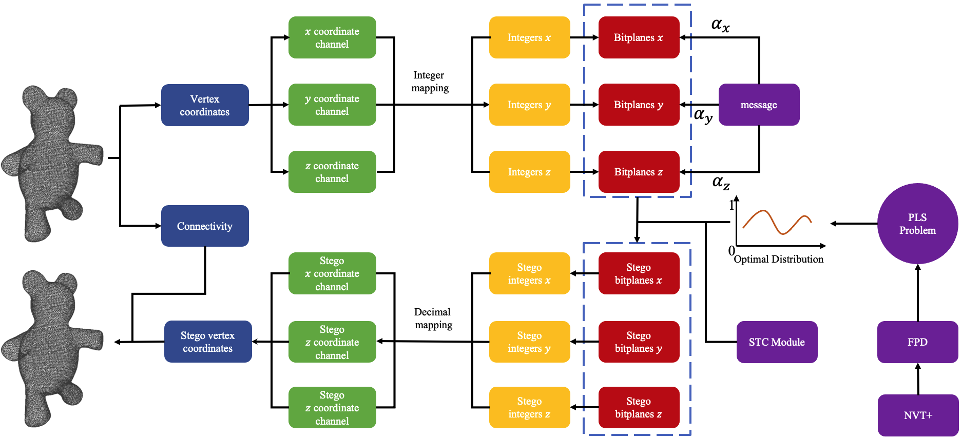
Figure 1: Message embedding pipeline of the proposed adaptive 3D mesh steganographic algorithm based on feature-preserving distortion.

3 Proposed Algorithm

3.1 Overall Framework

The framework of our 3D Mesh steganography is illustrated in Fig. 1. Given a mesh model, we first convert its vertex coordinates to integers and obtain bitplanes to construct the embedding domain (see Section 3.3). Secondly, to calculate the optimal vertex-changing distribution, we construct a payload limited sender (PLS) problem tailored for 3D mesh steganography (see Section 3.2) and construct FPD (see Section 3.4 for details). However, the calculation of FPD is exceptionally time-consuming, so we propose an improved FPD (IFPD) (see Section 3.5). By virtue of the optimal distribution, we adopt the $Q$-layered STC to embed practical messages into cover bitplanes (see Section 3.6). After obtaining the stego bitplanes, we adopt a decimal transformation and generate the stego mesh. Note that meshes used in this work are all composed of triangular faces unless otherwise stated.

3.2 Construction of PLS Problem

Given a mesh $\boldsymbol{M}=\{\boldsymbol{V},\boldsymbol{E},\boldsymbol{F}\}\in\boldsymbol{\mathcal{M}}$, we let $\boldsymbol{V}=\{\boldsymbol{v}_{i}\}_{i=1}^{|\boldsymbol{V}|}\in\{\mathbb{R}^{3}\}^{|\boldsymbol{V}|}$ be the vertex set of $\boldsymbol{M}$, where $\boldsymbol{v}_{i}=[v_{i,x},v_{i,y},v_{i,z}]^{\top}$. The edge set and face set of $\boldsymbol{M}$ are denoted by $\boldsymbol{E}=\{\boldsymbol{e}_{i}\}_{i=1}^{|\boldsymbol{E}|}$ and $\boldsymbol{F}=\{\boldsymbol{f}_{i}\}_{i=1}^{|\boldsymbol{F}|}$, respectively.

For our algorithm, message embedding will cause the vertices of $\boldsymbol{M}$ to move, inevitably distorting $\boldsymbol{M}$. Suppose embedding changes at vertices do not interact and embedding changes in one coordinate channel do not affect those of other channels. The total distortion can be measured in an additive way as follows.

$$D(\boldsymbol{M},\widetilde{\boldsymbol{M}})=\sum_{j\in\{x,y,z\}}\sum_{i=1}^{|\boldsymbol{V}|}\rho(v_{i,j}+\delta_{i,j}),\delta_{i,j}\in\mathbb{R},$$ (1)

where $\widetilde{\boldsymbol{M}}=\{\widetilde{\boldsymbol{V}},\widetilde{\boldsymbol{E}},\widetilde{\boldsymbol{F}}\}$ is the stego mesh, $\delta_{i,j}$ is the change quantity of $v_{i,j}$, and $\rho\geq 0$ denotes the cost function. Note $\boldsymbol{M}$ is given in advance and the proposed algorithm does not alter the topology of $\boldsymbol{M}$, implying $\boldsymbol{E}=\widetilde{\boldsymbol{E}}$ and $\boldsymbol{F}=\widetilde{\boldsymbol{F}}$. Therefore, we can rewrite $D(\boldsymbol{M},\widetilde{\boldsymbol{M}})$ as $D(\widetilde{\boldsymbol{V}})$ where $\widetilde{\boldsymbol{V}}=\{\tilde{\boldsymbol{v}}_{i}\}_{i=1}^{|\widetilde{\boldsymbol{V}}|}$, $\tilde{\boldsymbol{v}}_{i}=[\tilde{v}_{i,x},\tilde{v}_{i,y},\tilde{v}_{i,z}]^{\top}$, and $\tilde{v}_{i,j}=v_{i,j}+\delta_{i,j}$. Likewise, we write $\rho(v_{i,j}+\delta_{i,j})$ as $\rho(\delta_{i,j})$ for brevity. Given a relative payload $\alpha=\frac{m}{|\boldsymbol{V}|}$, where $m$ is the message size, we can minimize the expectation of Eq. (1) to obtain the optimal vertex-changing distribution as below.

$$\mathop{\rm{minimize}}_{\pi}\ E_{\pi}[D]=\sum_{j\in\{x,y,z\}}\sum_{i=1}^{|\boldsymbol{V}|}\int_{\mathbb{R}}\rho(\delta_{i,j})\pi(\delta_{i,j})\rm{d}\delta_{i,j},$$ (2)

$$\begin{aligned} &\mathop{\rm{s.t.}}\ H(\pi)=-\sum_{j\in\{x,y,z\}}\sum_{i=1}^{|\boldsymbol{V}|}\int_{\mathbb{\mathbb{R}}}\rm{ln}(\pi(\delta_{i,j}))\pi(\delta_{i,j})\rm{d}\delta_{i,j}=\alpha|\widetilde{\boldsymbol{V}}|,\\ &\sum_{j\in\{x,y,z\}}\alpha_{j}=\alpha,\end{aligned}$$

Where $\pi(\delta_{i,j})$ is the probability of $\delta_{i,j}$ occurring and $H(\pi)$ is the information entropy w.r.t. $\pi$.

Eq. (2) is also known as the PLS problem, and obviously, it can be regarded as three independent optimization problems w.r.t. $x$,$y$, and $z$ coordinate channels, respectively. However, calculating the optimal $\pi$ is not easy work because $\delta_{i,j}$ is a continuous variable and $\rho$ is not explicitly defined yet.

3.3 Construction of Embedding Domain

Vertex coordinates of uncompressed meshes are usually specified as floating point numbers conforming to IEEE 754 standard format [6, 22, 41] and in most cases, the vertex coordinates are represented in decimal form. Based on this fact, we construct the embedding domain as follows.

Integer mapping (IM). The coordinate component values of $\boldsymbol{v}_{i}$ typically retain limited significant digits, e.g., $\boldsymbol{v}_{i}=[0.172345,0.267324,0.563521]^{\top}$. This means we can always find a minimum $k_{j}\in\mathbb{N}$ satisfying $\ddot{v}_{i,j}=v_{i,j}\times 10^{k_{i,j}}\in\mathbb{Z}$. For a mesh $\boldsymbol{M}$, let $k^{*}=max\{k_{i,j}|i\in\{1,\cdots,|\boldsymbol{V}|\},j\in\{x,y,z\}\}$. In this way, the IM shown in Fig. 1 can be realized by $\ddot{v}_{i,j}=v_{i,j}\times 10^{k^{*}}$.

Bitplane acquisition (BA). After obtaining $k^{*}$, we can readily find a minimum $h^{*}\in\mathbb{N}^{*}$ satisfying $0\leq\ddot{v}_{i,j}\leq 2^{h^{*}}-1$. Let $b_{i,j}^{(l)}$ be the $l$-th least significant bit of $\ddot{v}_{i,j}$ and bitplane $\boldsymbol{B}_{j}^{(l)}=\{b_{i,j}^{(l)}\}_{i=1}^{|\boldsymbol{V}|}$. The embedding domain can be expressed as $\{\boldsymbol{B}_{j}^{(l)}|j\in\{x,y,z\},l\in\{1,\cdots,h^{*}\}\}$.

Decimal mapping (DM). Our message embedding is implemented by modifying bitplanes bits, which is equivalent to adding integer vectors to $\ddot{\boldsymbol{v}}_{i}$. Accordingly, the stego vertices can be obtained by DM

$$\tilde{\boldsymbol{v}}_{i}=\begin{bmatrix}\tilde{v}_{i,x}\\ \tilde{v}_{i,y}\\ \tilde{v}_{i,z}\end{bmatrix}=\begin{bmatrix}(\ddot{v}_{i,x}+\lfloor\delta_{i,x}\times 10^{k^{*}}\rfloor)/10^{k^{*}}\\ (\ddot{v}_{i,y}+\lfloor\delta_{i,y}\times 10^{k^{*}}\rfloor)/10^{k^{*}}\\ (\ddot{v}_{i,z}+\lfloor\delta_{i,z}\times 10^{k^{*}}\rfloor)/10^{k^{*}}\end{bmatrix}.$$ (3)

Discretization. $\delta_{i,j}\times 10^{k^{*}}$ may be decimals because $\delta_{i,j}\in\boldsymbol{\mathbb{R}}$ is a continuous variable. However, modifications on bitplanes will never cause coordinate changes in decimal form, and thus we select to round down $\delta_{i,j}\times 10^{k^{*}}$, which can be regarded as discretizing $\delta_{i,j}$ directly. Let $\delta_{i,j}\in\boldsymbol{I}\subset\{\delta/10^{k^{*}}|\delta\in\mathbb{Z}\}$. The cardinality of $\boldsymbol{I}$ will not be set too large because we do not want the message embedding to bring about perceptible mesh distortion. In this way, we can rewrite Eq. (2) as below.

$$\mathop{\rm{minimize}}_{\pi}\ E_{\pi}[D]=\sum_{j\in\{x,y,z\}}\sum_{i=1}^{|\boldsymbol{V}|}\sum_{\delta_{i,j}\in\boldsymbol{I}}\rho(\delta_{i,j})\pi(\delta_{i,j})$$ (4)

$$\begin{aligned} &\mathop{\rm{s.t.}}\ H(\pi)=-\sum_{j\in\{x,y,z\}}\sum_{i=1}^{|\boldsymbol{V}|}\sum_{\delta_{i,j}\in\boldsymbol{I}}\rm{ln}(\pi(\delta_{i,j}))\pi(\delta_{i,j})=\alpha|\boldsymbol{V}|,\\ &\sum_{j\in\{x,y,z\}}\alpha_{j}=\alpha.\end{aligned}$$

The optimal $\pi$ has a form of Gibbs distribution [23], namely

$$\pi(\delta_{i,j})=\frac{e^{-\lambda_{j}\rho(\delta_{i,j})}}{\sum_{\delta\in\boldsymbol{I}}e^{-\lambda_{j}\rho(\delta)}},j\in\{x,y,z\},\\$$ (5)

where $\lambda_{j}$ is a scalar calculated through an iterative search with the condition $H(\pi)=\alpha_{j}|\boldsymbol{V}|$. Once $\rho$ is determined, we can calculate the optimal $\pi$ by optimizing Eq. (4).

3.4 Design of FPD

3.4.1 Selection of Efficient Steganalytic Features

The advent of a new information security technique is bound to be met with corresponding attacks, and the game between attacker and defender promotes the expected progress of both sides. Based on this point, we believe that well-performed steganalyzers can help to design more secure steganography. In 3D steganalysis, NVT+, a 100-dimensional feature set $\boldsymbol{\Phi}=\{\phi_{i}\}^{100}_{i=1}$, has been demonstrated experimentally to possess the best steganalysis performance [14, 25]. While completely preserving mesh features during the embedding is alluring, it is rather difficult to achieve in reality. Therefore, we should clarify which sub-features of NVT+ are effective enough for steganalysis. The detailed analysis of NVT+ sub-features is presented in Appendix A. Here we directly offer a conclusion that sub-features $\phi_{1}\!\sim\!\phi_{12}$, $\phi_{33}\!\sim\!\phi_{36}$, $\phi_{65}\!\sim\!\phi_{76}$, $\phi_{77}\!\sim\!\phi_{88}$, and $\phi_{89}\!\sim\!\phi_{100}$ may be useful for the distortion design.

TABLE I: A list of unnormalized change costs of several vertices on a plane under sub-feature $\phi_{33}\!\sim\!\phi_{36}$.

	-6	-5	-4	-3	-2	-1	-0	1	2	3	4	5	6
PSB-346.off
$v_{2601,x}$	0	0	0	0	0	0	0	0	0	0	0	0	0
$v_{3455,y}$	3.9969	3.9887	3.9781	3.9637	3.9418	3.9003	0	3.9003	3.9418	3.9637	3.9781	3.9887	3.9969
$v_{3455,z}$	0	0	0	0	0	0	0	0	0	0	0	0	0
PSB-347.off
$v_{1859,x}$	0	0	0	0	0	0	0	0	0	0	0	0	0
$v_{1859,y}$	0	0	0	0	0	0	0	0	0	0	0	0	0
$v_{1859,z}$	5.8171	5.8027	5.7844	5.7596	5.7223	5.6524	0	5.6524	5.7223	5.7596	5.7844	5.8027	5.8171
PSB-153.off
$v_{3362,x}$	0.0835	0.0869	0.0911	0.0963	0.1034	0.1147	0	0.1147	0.1034	0.0963	0.0911	0.0869	0.0835
$v_{3362,y}$	0	0	0	0	0	0	0	0	0	0	0	0	0
$v_{3362,z}$	0	0	0	0	0	0	0	0	0	0	0	0	0
PSB-104.off
$v_{3119,x}$	0	0	0	0	0	0	0	0	0	0	0	0	0
$v_{3119,y}$	0	0	0	0	0	0	0	0	0	0	0	0	0
$v_{3119,z}$	0.3445	0.3476	0.3512	0.3556	0.3616	0.3707	0	0.3738	0.3616	0.3556	0.3512	0.3476	0.3445

3.4.2 Design of Cost Function

Without loss of generality, we choose the first $L$ best sub-features from NVT+ to construct the cost function $\rho$ as below.

$$\rho(\delta_{i,j})=\mu\sum_{k=1}^{L}N_{or}(||S_{k}(\boldsymbol{M})-S_{k}(\widetilde{\boldsymbol{M}}(\delta_{i,j}))||_{1})$$ (6)

where $S_{k}:\boldsymbol{\mathcal{M}}\rightarrow\boldsymbol{\mathbb{R}}^{d_{k}}$ denotes the feature extractor corresponding to the $k$-th sub-feature; $d_{k}$ is the dimension of the feature vector extracted by $S_{k}$; $\widetilde{\boldsymbol{M}}(v_{i,j})$ denotes that only $v_{i,j}$ in $\boldsymbol{M}$ is altered and its change quantity is $\delta_{i,j}$; $N_{or}(\cdot)$ is the normalization function; $\mu>0$ is a scale factor set to prevent numerical calculation issues. Note that $N_{or}$ is indispensable because different steganalytic sub-features are derived from different geometric features, whose values may be of diverse magnitude orders. $N_{or}$ can effectively balance the effect of each sub-feature on FPD. By substituting Eq. (6) into Eq. (1), we can get the specific form of FPD. Minimizing FPD helps preserve steganalytic and local and global geometric features to a certain extent, which is well demonstrated in the later experiments.

3.5 Improvement to FPD

3.5.1 Analysis of Sub-features $\phi_{1}\!\sim\!\phi_{12}$ and $\phi_{33}\!\sim\!\phi_{36}$

The steganalysis performance of $\phi_{1}\sim\phi_{12}$ and $\phi_{33}\sim\phi_{36}$ on the PSB and PMN datasets exposes their common problem, that is, the lack of generalization for meshes from different datasets. Therefore, using the two sub-features to design the distortion function will likely cause our algorithm to favour some kind of mesh, contrary to the concept of good distortion design. Furthermore, the following proposition holds.

Proposition 1

$\phi_{33}\!\sim\!\phi_{36}$ exhibits good resistance to steganalysis on the PSB dataset but is unsuitable for distortion design.

Proof:

The simplest way to prove it is to show some specific cases where $\phi_{33}\!\sim\!\phi_{36}$ does not apply to steganography. We find that modifying the coordinates of vertices on a plane may not cause changes in dihedral angle-related features. As illustrated in Fig. 2, if we move $\boldsymbol{v}_{i}$ towards $\boldsymbol{v}_{i+1}$ along $\boldsymbol{e}_{i}$ on the plane, the dihedral angle between every two contiguous faces in the such plane will not change. This means, for any vertex $\boldsymbol{v}_{i}$ on the plane, as long as the movements of $\boldsymbol{v}_{i}$ do not lead to it leaving the plane, then $\rho(\delta_{i,j})\equiv 0$ (only $\phi_{33}\sim\phi_{36}$ is considered in $\rho$), which is not what we expect. Table I shows the phenomenon. Such vertex movements will inevitably bring about changes in mesh features. Furthermore, as long as meshes contain planar regions, it is not difficult to find such vertex movements.

All in all, we will not consider $\phi_{1}\!\sim\!\phi_{12}$ and $\phi_{33}\!\sim\!\phi_{36}$ in FPD. ∎

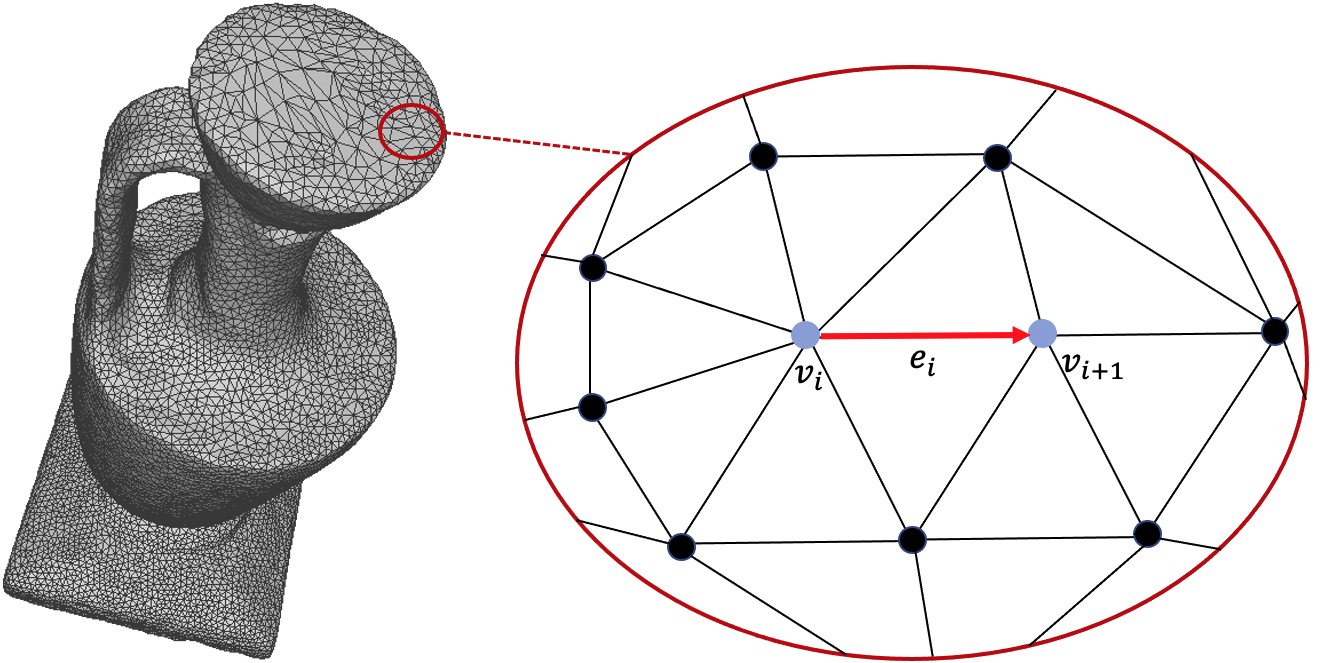
Figure 2: A case where vertex movements without changing the dihedral angle related features.

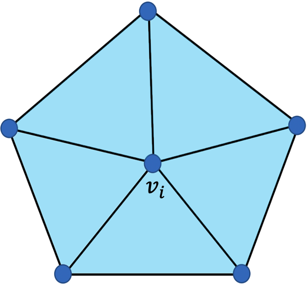
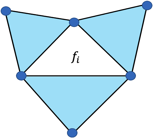
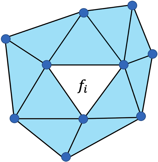
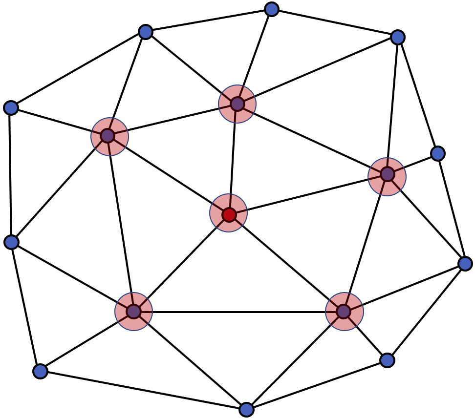
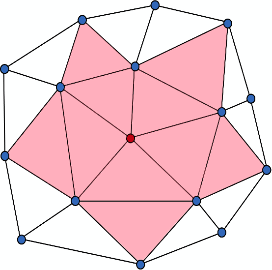
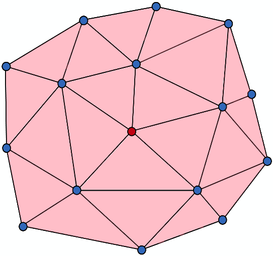
Figure 3: llustration of diverse neighborhood patterns and their respective vertex influence regions. (a) $\mathcal{N}_{1}(\boldsymbol{v}_{i})$ contains 1-ring neighboring faces of $\boldsymbol{v}_{i}$. (b) $\mathcal{N}_{2}(\boldsymbol{f}_{i})$ contains faces that share edges with $\boldsymbol{f}_{i}$. (c) $\mathcal{N}_{3}(\boldsymbol{f}_{i})$ contains faces that share vertices with $\boldsymbol{f}_{i}$. (d), (e), and (f) are the visualizations of vertex influence domain corresponding to (a), (b), and (c) respectively. The modified vertices are marked in red and the vertex influence domain is painted pink.

3.5.2 Analysis of Sub-features $\phi_{65}\!\sim\!\phi_{76}$, $\phi_{77}\!\sim\!\phi_{88}$, and $\phi_{89}\!\sim\!\phi_{100}$

In contrast to $\phi_{1}\!\sim\!\phi_{12}$ and $\phi_{33}\!\sim\!\phi_{36}$, the three sub-features perform well on both datasets and besides, it is hard to move $\boldsymbol{v}_{i}$ in a way that results in $\rho(\delta_{i,j})\equiv 0$ (only the three sub-features are considered in $\rho$), which is because the three sub-features are based on the second-order local description of mesh surfaces. From this point of view, using them for constructing FPD makes sense.

Calculating $\rho(\delta_{i,j})$ with the method in [14]. Let $S_{k},k\in\{1,2,3\}$, be the feature extractors of the three sub-features, respectively. [14] proposes three normal voting tensors corresponding to the three sub-features respectively, whose expressions are given by

$$\boldsymbol{\rm{T}}_{1,i}=\sum_{\boldsymbol{f}\in\boldsymbol{\mathcal{N}}_{1}(\boldsymbol{v}_{i})}W_{1,i}\boldsymbol{n}_{\boldsymbol{f}}\cdot\boldsymbol{n}_{\boldsymbol{f}}^{\top},i\in\{1,\cdots,|\boldsymbol{V}|\},$$ (7)

$$\boldsymbol{\rm{T}}_{2,i}=\sum_{\boldsymbol{f}\in\boldsymbol{\mathcal{N}}_{2}(\boldsymbol{f}_{i})}W_{2,i}\boldsymbol{n}_{\boldsymbol{f}}\cdot\boldsymbol{n}_{\boldsymbol{f}}^{\top},i\in\{1,\cdots,|\boldsymbol{F}|\},$$

$$\boldsymbol{\rm{T}}_{3,i}=\sum_{\boldsymbol{f}\in\boldsymbol{\mathcal{N}}_{3}(\boldsymbol{f}_{i})}W_{3,i}\boldsymbol{n}_{\boldsymbol{f}}\cdot\boldsymbol{n}_{\boldsymbol{f}}^{\top},i\in\{1,\cdots,|\boldsymbol{F}|\}.$$

$\boldsymbol{\mathcal{N}}_{1}$, $\boldsymbol{\mathcal{N}}_{2}$, and $\boldsymbol{\mathcal{N}}_{3}$ represent three diverse neighborhood patterns (see Fig. 3 (a)-(c)). $\boldsymbol{n}_{\boldsymbol{f}}$ denotes the normal of face $\boldsymbol{f}$. The weights $W_{k,i}$ are defined in [14]. Regarding the implementation of $S_{k}$, for brevity, we omit the subscript $k$. Let $\lambda_{i}^{(1)},\lambda_{i}^{(2)}$, and $\lambda_{i}^{(3)}$ be the three eigenvalues of $\boldsymbol{\rm{T}}_{i}$, $i\in\{1,\cdots,N_{\lambda}\}$, and $\lambda_{i}^{(1)}\geq\lambda_{i}^{(2)}\geq\lambda_{i}^{(3)}\geq 0$. Eq. (7) tells us if $k=1$, $N_{\lambda}=|\boldsymbol{V}|$, otherwise $N_{\lambda}=|\boldsymbol{F}|$. The eigenvalues of all $\boldsymbol{\rm{T}}_{i}$ can form three sets, namely $\boldsymbol{\lambda}_{1}=\{\lambda^{(1)}_{i}-\lambda^{(2)}_{i}\}_{i=1}^{N_{\lambda}}$, $\boldsymbol{\lambda}_{2}=\{\lambda^{(2)}_{i}-\lambda^{(3)}_{i}\}_{i=1}^{N_{\lambda}}$, and $\boldsymbol{\lambda}_{3}=\{\lambda^{(3)}_{i}\}_{i=1}^{N_{\lambda}}$. For meshes $\boldsymbol{M}$ and $\widetilde{\boldsymbol{M}}(\delta_{i,j})$, [14] calculates their respective residuals as

$$\begin{aligned} &\boldsymbol{r}_{i}=log(abs(\boldsymbol{\lambda}_{i}-SM(\boldsymbol{\lambda}_{i})))\\ &\tilde{\boldsymbol{r}}_{i}=log(abs(\tilde{\boldsymbol{\lambda}}_{i}-SM(\tilde{\boldsymbol{\lambda}}_{i})))\end{aligned}\ \ i\in\{1,2,3\},$$ (8)

where $SM$ is the smoothing function mentioned in [14] and $abs$ is the element-wise absolute value function. The post-procedure to generate $S(\boldsymbol{M})$ and $S(\widetilde{\boldsymbol{M}}(\delta_{i,j}))$ is of no interest to this paper. By repeating the above operation, we can get $\rho(\delta_{i,j})$ for all vertices and $\delta_{i,j}\in\boldsymbol{I}$.

An improved method. However, the above method is highly time-consuming, as shown in Table II.

Definition 1 (Vertex influence domain)

Under the neighborhood pattern $\mathcal{N}_{k}$, the vertex influence domain of $\boldsymbol{v}_{i}$ (denoted by $\boldsymbol{ID}_{k,i}$) is a set containing $\boldsymbol{\rm{T}}_{k,i}$ whose eigenvalues will be changed when $\boldsymbol{v}_{i}$ is moved.

Proposition 2

Given a mesh $\boldsymbol{M}$ with large $|\boldsymbol{V}|$ and $|\boldsymbol{F}|$, for any vertex $\boldsymbol{v}_{i}$, we have $|\boldsymbol{ID}_{k,i}|\ll N_{\lambda}$.

Proof:

Moving $\boldsymbol{v}_{i}$ only affects the attributes (e.g., area and face normal) of its 1-ring neighboring faces. Moreover, Eq. (7) and Fig. 3 (a)-(c) tell us that $\boldsymbol{\rm{T}}_{k,i}$ is only determined by the attributes of faces in its relevant neighborhood. The number of faces in either of the above neighborhoods is far less than $|\boldsymbol{V}|$ and $|\boldsymbol{F}|$, indicating that the influence domain of $\boldsymbol{v}_{i}$ is minimal. ∎

Proposition 3

Given a mesh $\boldsymbol{M}$ and its smoothed version $SM(\boldsymbol{M})$, making full use of $\boldsymbol{ID}_{k,i}$ of $\boldsymbol{v}_{i}$ can help to speed up the calculation of $\rho(\delta_{i,j})$.

Proof:

Since only one vertex of $\boldsymbol{M}$ is moved, $SM(\boldsymbol{M})$ is mighty similar to $SM(\widetilde{\boldsymbol{M}}(\delta_{i,j}))$, and thus it is reasonable to assume $SM(\boldsymbol{\lambda}_{i})=SM(\tilde{\boldsymbol{\lambda}}_{i})$ in Eq. (8). Based on this assumption, suppose we already know the eigenvalues of $\boldsymbol{M}$ and $SM(\boldsymbol{M})$, we can readily obtain the residuals $\boldsymbol{r}_{i}$ with Eq. (8). According to Definition 1 and Proposition 2, to obtain $\tilde{\boldsymbol{r}}_{i}$ of $\widetilde{\boldsymbol{M}}(\delta_{i,j})$, all we need to do is recalculate the eigenvalues of tensors in $\boldsymbol{ID}_{k,i}$ and substitute the corresponding part of the eigenvalues of $\boldsymbol{M}$ with them. This method avoids many needless calculations on eigenvalues and $SM(\tilde{\boldsymbol{\lambda}}_{i})$, boosting the calculation of $\rho(\delta_{i,j})$ for all vertices and $\delta_{i,j}\in\boldsymbol{I}$ dramatically. ∎

Visualization of vertex influence domain. The last remaining issue is how to visually show $\boldsymbol{ID}_{k,i}$. According to Eq. (7), let $\boldsymbol{\rm{T}}_{1,i}$, $\boldsymbol{\rm{T}}_{2,i}$, and $\boldsymbol{\rm{T}}_{3,i}$ be associated with $\boldsymbol{v}_{i}$, $\boldsymbol{f}_{i}$ , and $\boldsymbol{f}_{i}$ respectively. By establishing these associations, we can give intuitive expressions of $\boldsymbol{ID}_{k,i}$ w.r.t. $\boldsymbol{v}_{i}$ as below.

$$\boldsymbol{ID}_{1,i}=\{\boldsymbol{v}\mid\boldsymbol{v}\in\boldsymbol{f},\boldsymbol{f}\in\mathcal{N}_{1}(\boldsymbol{v}_{i})\},$$ (9)

$$\boldsymbol{ID}_{2,i}=\{\boldsymbol{f}\mid\boldsymbol{f}\in\mathcal{N}_{2}(\boldsymbol{f}^{\star}),\boldsymbol{f}^{\star}\in\mathcal{N}_{1}(\boldsymbol{v}_{i})\},$$

$$\boldsymbol{ID}_{3,i}=\{\boldsymbol{f}\mid\boldsymbol{f}\in\mathcal{N}_{3}(\boldsymbol{f}^{\star}),\boldsymbol{f}^{\star}\in\mathcal{N}_{1}(\boldsymbol{v}_{i})\}.$$

The visualization results of $\boldsymbol{ID}_{1,i}$, $\boldsymbol{ID}_{2,i}$, and $\boldsymbol{ID}_{3,i}$ are shown in Fig. 3 (d)-(e), respectively.

3.6 Implementation of Message Embedding and Retrieval

3.6.1 Calculation of BMP

$Q$-layered STC is the most commonly used steganographic coding due to its near-optimal performance for arbitrary distortion functions [24]. While the technique has been highly mature in image steganography, applying it to 3D mesh steganography is still challenging.

Brief review of $Q$-layered STC. According to [24], the value of $Q$ is determined by

$$Q=\inf\mathop{\arg\max}_{q\in\boldsymbol{\mathbb{N}}^{*}}[|\boldsymbol{I}|\leq 2^{q}],$$ (10)

where $[\cdot]$ is the Inverson bracket. Eq. (10) implies that only $Q$ bits are needed to uniquely represent each element of $\boldsymbol{I}$. When the message embedding occurs, the embedding capacity of $\boldsymbol{v}_{i}$ is $\sum_{j\in\{x,y,z\}}\sum_{l=1}^{Q}H(\tilde{b}_{i,j}^{(l)}|\tilde{b}_{i,j}^{(l-1)},\cdots,\tilde{b}_{i,j}^{(1)})$, where $\tilde{b}_{i,j}^{(l)}$ is the stego version of $b_{i,j}^{(l)}$.

Issue statement. $H(\tilde{b}_{i,j}^{(l)}|\tilde{b}_{i,j}^{(l-1)},\cdots,\tilde{b}_{i,j}^{(1)})$ is determined by the BMP $P(\tilde{b}_{i,j}^{(l)}|\tilde{b}_{i,j}^{(l-1)},\cdots,\tilde{b}_{i,j}^{(1)})$. In [24], the authors only provide a manual approach to calculating $P(\tilde{b}_{i,j}^{(l)}|\tilde{b}_{i,j}^{(l-1)},\cdots,\tilde{b}_{i,j}^{(1)})$, which will be increasingly complex as $Q$ gets larger. In addition, the approach will be inflexible when $Q$ varies. In their code library, only source codes tailored for binary, ternary, and pentary embedding examples are given, which are far from satisfying our algorithm’s need for embedding capacity. Therefore, we propose a universal and automatic approach to calculating $P(\tilde{b}_{i,j}^{(l)}|\tilde{b}_{i,j}^{(l-1)},\cdots,\tilde{b}_{i,j}^{(1)})$ more flexibly and conveniently.

Our approach. Since $b_{i,j}^{(l)},\tilde{b}_{i,j}^{(l)}\in\{0,1\}$, we can construct a complete binary tree with $Q+1$ layers to solve $P(\tilde{b}_{i,j}^{(l)}|\tilde{b}_{i,j}^{(l-1)},\cdots,\tilde{b}_{i,j}^{(1)})$. For the $l$-th layer of the complete binary tree ($l\in[2,Q+1]$ because the root node is spared for other uses), we specify each left child node to store $P(\tilde{b}_{i,j}^{(l-1)}=0|\tilde{b}_{i,j}^{(l-2)},\cdots,\tilde{b}_{i,j}^{(1)})$ and each right one to store the opposite probability. As described in [24], before performing message embedding on $b_{i,j}^{(l-1)}$, we know the values of $\tilde{b}_{i,j}^{(l-2)},\cdots,\tilde{b}_{i,j}^{(2)}$, and $\tilde{b}_{i,j}^{(1)}$. That is to say, only one node in each of the previous $l\!-\!1$ layers, except for the root node, is responsible for the solution of $P(\tilde{b}_{i,j}^{(l-1)}|\tilde{b}_{i,j}^{(l-2)},\cdots,\tilde{b}_{i,j}^{(1)})$. Based on this point, we set an array $\boldsymbol{A}$ of length $Q+1$, as shown in Fig. 4, for data storage to reduce the spatial complexity. Let $P_{ar}^{(l)}(\cdot)$ represents the $l$-th least significant bit of a given integer. The first element of $\boldsymbol{A}$, which is initially set to 1, is used to store the probability $P(\tilde{b}_{i,j}^{(l-2)},\cdots,\tilde{b}_{i,j}^{(1)})$. It is straightforward to derive $P(\tilde{b}_{i,j}^{(l-1)}=0,\tilde{b}_{i,j}^{(l-2)},\cdots,\tilde{b}_{i,j}^{(1)})$, whose value is the sum of elements in

$$\boldsymbol{\Pi}_{i,j}^{(l)}(0)=\{\pi({\delta_{i,j}})|\delta_{i,j}\in\boldsymbol{I},$$ (11)

$$\pi(\delta_{i,j})\in\boldsymbol{\Pi}_{i,j}^{(l-1)},P_{ar}^{(l-1)}(\ddot{v}_{i,j}+\delta_{i,j}\times 10^{k^{*}})=0\}.$$

$\boldsymbol{\Pi}_{i,j}^{(l)}(1)=\boldsymbol{\Pi}_{i,j}^{(l-1)}\setminus\boldsymbol{\Pi}_{i,j}^{(l)}(0)$. $\boldsymbol{\Pi}_{i,j}^{(l-1)}$ is a iteratively-obtained probability set. According to the total probability formula, we can easily work out $P(\tilde{b}_{i,j}^{(l-1)}=0|\tilde{b}_{i,j}^{(l-2)},\cdots,\tilde{b}_{i,j}^{(1)})$ and $P(\tilde{b}_{i,j}^{(l-1)}=1|\tilde{b}_{i,j}^{(l-2)},\cdots,\tilde{b}_{i,j}^{(1)})$, and then perform 1-layered STC on $\boldsymbol{B}_{j}^{(l-1)}=\{b_{i,j}^{(l-1)}\}_{i=1}^{|\boldsymbol{V}|}$ to generate $\widetilde{\boldsymbol{B}}_{j}^{(l-1)}$. After that, if $\tilde{b}^{(l-1)}_{i,j}=0$, we set $\boldsymbol{\Pi}_{i,j}^{(l)}=\boldsymbol{\Pi}_{i,j}^{(l)}(0)$, otherwise $\boldsymbol{\Pi}_{i,j}^{(l)}=\boldsymbol{\Pi}_{i,j}^{(l)}(1)$. $\boldsymbol{\Pi}_{i,j}^{(l)}$ will be used for the next bitplane. Note that the 1-layered STC follows the flipping lemma proposed in [24]. The pseudo-code of our approach is given in Algorithm 1. Fig. 4 illustrates an intuitive embedding case for Algorithm 1 with $\{b_{i,j}^{(2)},b_{i,j}^{(1)}\}=\{0,1\}$ and $\boldsymbol{I}=\{\frac{-1}{10^{k^{*}}},0,\frac{1}{10^{k^{*}}}\}$. The red arrow lines depict a bit modification path that we assume.

Merits of our approach. Algorithm 1 shows that our approach requires only a few parameters as input. Furthermore, when we alter $Q$ due to the payload change, it can still flexibly cope with the probability calculation without manual intervention.

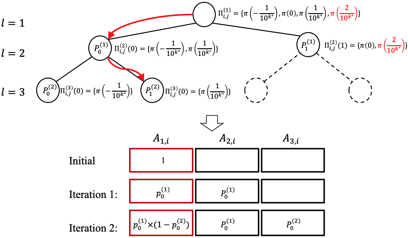
Figure 4: Illustration of the probability-solving process w.r.t. $\boldsymbol{I}=\{\frac{-1}{10^{k^{*}}},0,\frac{1}{10^{k^{*}}}\}$ and $\{b_{i,j}^{(2)},b_{i,j}^{(1)}\}=\{0,1\}$. The probability marked in red is an additional element whose value is 0 in this case. The red arrow lines depict our assumed bit modification path.

Algorithm 1 Universal and Automatic BMP Calculation Approach for $Q$-layered STC

Input: Bitplane set $\boldsymbol{B}_{j}=\{\boldsymbol{B}_{j}^{(l)}\}_{l=1}^{h^{*}}$, $\boldsymbol{I}$, optimal distribution $\boldsymbol{\Pi}_{j}=\{\boldsymbol{\Pi}_{i,j}\}_{i=1}^{|\boldsymbol{V}|}$, where $\boldsymbol{\Pi}_{i,j}=\{\pi(\delta_{i,j})\mid\delta_{i,j}\in\boldsymbol{I}\}$.
  Output: $\boldsymbol{A}$, $\widetilde{\boldsymbol{B}}_{j}$.

1:Obtain $Q$ with Eq. (10);

2:Fill $\boldsymbol{I}$ to make $|\boldsymbol{I}|=2^{Q}$ and set corresponding probability of the filling elements to 0;

3:Create an array $\boldsymbol{A}$ of size $(Q+1)\times|\boldsymbol{V}|$ and set $\boldsymbol{A}_{1,:}=1$;

4:Set $\boldsymbol{\Pi}_{:,j}^{(1)}=\boldsymbol{\Pi}_{:,j}$;

5:for $l=2$ to $Q+1$ do

6:     for $i=1$ to $|\boldsymbol{V}|$ do

7:         Obtain $\boldsymbol{\Pi}_{i,j}^{(l)}(0)$ with Eq. (11) and $\boldsymbol{\Pi}_{i,j}^{(l)}(1)=\boldsymbol{\Pi}_{i,j}^{(l-1)}\setminus\boldsymbol{\Pi}_{i,j}^{(l)}(0)$ ;

8:         Calculate $P(\tilde{b}_{i,j}^{(l-1)}=0,\tilde{b}_{i,j}^{(l-2)},\cdots,\tilde{b}_{i,j}^{(1)})$ by adding elements in $\boldsymbol{\Pi}_{i,j}^{(l)}(0)$ together;

9:         $\boldsymbol{A}_{l,i}=P(\tilde{b}_{i,j}^{(l-1)}=0,\tilde{b}_{i,j}^{(l-1)},\cdots,\tilde{b}_{i,j}^{(1)})/\boldsymbol{A}_{1,i}$;      

10:     Perform 1-layered STC on $\boldsymbol{B}_{j}^{(l-1)}$ to generate $\widetilde{\boldsymbol{B}}_{j}^{(l-1)}$;

11:     for $i=1$ to $|\boldsymbol{V}|$ do

12:         if $\tilde{b}_{i,j}^{(l-1)}=0$ then

13:              $\boldsymbol{\Pi}_{i,j}^{(l)}=\boldsymbol{\Pi}_{i,j}^{(l)}(0)$;

14:         else

15:              $\boldsymbol{\Pi}_{i,j}^{(l)}=\boldsymbol{\Pi}_{i,j}^{(l)}(1)$;          

16:         $\boldsymbol{A}_{1,i}=P(\tilde{b}_{i,j}^{(l-1)}\mid\tilde{b}_{i,j}^{(l-2)},\cdots,\tilde{b}_{i,j}^{(1)})\times A_{1,i}$;      

17:$\widetilde{\boldsymbol{B}}_{j}=\{\boldsymbol{B}^{(h^{*})}_{j},\cdots,\boldsymbol{B}^{(Q+1)}_{j},\widetilde{\boldsymbol{B}}^{(Q)}_{j},\cdots,\widetilde{\boldsymbol{B}}^{(1)}_{j}\}$;

18:return $\boldsymbol{A}$ and $\widetilde{\boldsymbol{B}}_{j}$.

Algorithm 2 Adaptive 3D Mesh Steganography Based on FPD

Input: Cover mesh $\boldsymbol{M}=\{\boldsymbol{V},\boldsymbol{E},\boldsymbol{F}\}$, quantization parameter $k^{*}$, bit number $h^{*}$, $\boldsymbol{I}$, payload $\alpha$.
  Output: Stego mesh $\widetilde{\boldsymbol{M}}$.

1:Divide $\alpha$ into $\alpha_{x}$, $\alpha_{y}$, and $\alpha_{z}$ ;

2:for $j$ in $\{x,y,z\}$  do

3:     Obtain $\ddot{\boldsymbol{V}}_{j}=\{\ddot{v}_{i,j}\}_{i=1}^{|\boldsymbol{V}|}$ with IM and $k^{*}$;

4:     Obtain Bitplane set $\boldsymbol{B}_{j}=\{\boldsymbol{B}_{j}^{(l)}\}_{l=1}^{h^{*}}$ with BA;

5:     Calculate $\rho(\delta_{i,j})$ for all vertices and $\delta_{i,j}\in\boldsymbol{I}$ with Eq. (6);

6:     Calculate the optimal distribution $\boldsymbol{\Pi}_{j}=\{\boldsymbol{\Pi}_{i,j}\}_{i=1}^{|\boldsymbol{V}|}$ with Eq. (4) and $\alpha_{j}$, where $\boldsymbol{\Pi}_{i,j}=\{\pi(\delta_{i,j})\mid\delta_{i,j}\in\boldsymbol{I}\}$;

7:     Input $\boldsymbol{B}_{j}$, $\boldsymbol{I}$, and $\boldsymbol{\Pi}_{j}$ to Algorithm 1 and obtain stego bitplane set $\widetilde{\boldsymbol{B}}_{j}$;

8:     Obtain $\widetilde{\boldsymbol{V}}_{j}=\{\tilde{v}_{i,j}\}_{i=1}^{|\boldsymbol{V}|}$ with DM and $k^{*}$;

9:Combine $\widetilde{\boldsymbol{V}}_{x}$, $\widetilde{\boldsymbol{V}}_{y}$, and $\widetilde{\boldsymbol{V}}_{z}$ as $\widetilde{\boldsymbol{V}}$;

10:Obtain $\widetilde{\boldsymbol{M}}=\{\widetilde{\boldsymbol{V}},\boldsymbol{E},\boldsymbol{F}\}$;

11:return $\widetilde{\boldsymbol{M}}$.

3.6.2 Message Embedding

We present the complete message embedding algorithm in Algorithm 2. Note that we regard the message embedding as three independent embedding tasks w.r.t. $x$, $y$, $z$ coordinate channels, respectively. In addition, we set $|\boldsymbol{I}|=2^{Q}$ and $\rho(\delta_{i,j})<\infty$ for $\delta_{i,j}\in\boldsymbol{I}$ to avoid wetness in each layer of $Q$-layered STC as much as possible. For more details of the wet paper codes, please refer to [24].

3.6.3 Message Retrieval

Since we adopt the $Q$-layered STC, the whole message embedding can be implemented by performing the 1-layered STC on a series of bitplanes apiece. Accordingly, the message retrieval on stego bitplanes can be expressed by

$$\boldsymbol{m}_{l,j}=\boldsymbol{\rm{H}}_{l,j}^{STC}\cdot\widetilde{\boldsymbol{B}}_{j}^{(l)},l\in\{1,2,\cdots,Q\},\ j\in\{x,y,z\},$$ (12)

where $\boldsymbol{\rm{H}}_{l,j}^{STC}\in\{0,1\}^{|\boldsymbol{m}_{l,j}|\times|\boldsymbol{V}|}$ denotes the parity-check matrix derived from a predesigned submatrix $\widehat{\boldsymbol{\rm{H}}}_{l,j}\in\{0,1\}^{h\times w}$. Typically, $6\leq h\leq 15$ and $\frac{1}{w+1}<\frac{|\boldsymbol{m}_{l,j}|}{|\boldsymbol{V}|}<\frac{1}{w}$. Note that $\boldsymbol{\rm{H}}_{l,j}^{STC}$ and the size of $\boldsymbol{m}_{l,j}$ are shared by the sender and recipient, and the height of $\widehat{\boldsymbol{\rm{H}}}_{l,j}$ is suggested to be set to a moderately large value according to [24].

4 Experimental Results and Analysis

4.1 Setup of Experiments

4.1.1 Datasets

All of experiments in this paper are conducted on the following three 3D mesh datasets:

• Princeton ModelNet (PMN): The dataset contains a comprehensive collection of 3D CAD models, which are drawn manually for researchers in computer graphics, computer vision, robotics, and cognitive science.

• Princeton Shape Benchmark (PSB): The dataset is composed of 400 watertight mesh models, which are collected from several web repositories. It is subdivided into 20 object categories, each of which contains 20 meshes.

• The Stanford Models (TSM): The dataset consists of several dense reconstructed mesh models, which are scanned by laser triangulation range scanners.

4.1.2 Criteria for Steganography

We evaluate our algorithm from three aspects:

• Steganographic Security: Steganographic security can also be referred to as undetectability, namely the anti-steganalysis ability. It is usually measured by test error. In this paper, we adopt the “out-of-bag” error $E_{OOB}$ [39] to evaluate security, whose expression is

  $$E^{(n)}_{OOB}=\frac{1}{2N^{data}}\sum_{i=1}^{N^{data}}(B^{(n)}(\boldsymbol{\Phi}_{i})+1-B^{(n)}(\widetilde{\boldsymbol{\Phi}}_{i})),$$ (13)

  where $\boldsymbol{\Phi}_{i}$ and $\widetilde{\boldsymbol{\Phi}}_{i}$ are cover and stego steganalytic features respectively; $n$ denotes the number of base learners used in the ensemble classifier; $B^{(n)}(\cdot)\in\{0,1\}$.

• Embedding Capacity: Embedding capacity in this paper is measured by the payload $\alpha$.

• Robustness: The ability to resist specified attacks, such as geometric attack and vertex reordering.

4.1.3 Experimental Environment

All experiments are conducted on a computer with Intel Xeon 5218R and 64GB RAM with Matlab 2019(a).

TABLE II: Costing complexity of partial meshes from PSB, PMN, and TSM using six cost funcitons in the case of $\boldsymbol{I}=\{-6/10^{k^{*}},\cdots,-1/10^{k^{*}},0,1/10^{k^{*}},\cdots,6/10^{k^{*}}\}$, respectively.

	Time (s)	OFPD-S1	IFPD-S1	OFPD-S2	IFPD-S2	OFPD-S3	IFPD-S3
	102.off (15724 vertices)	$\gg 3600$	414.0169	$\gg 3600$	813.1334	$\gg 3600$	761.1621
PSB	140.off (9200 vertices)	$\gg 3600$	153.5684	$\gg 3600$	286.1365	$\gg 3600$	276.4585
	325.off (14999 vertices	$\gg 3600$	337.3610	$\gg 3600$	739.2899	$\gg 3600$	700.6807å
	1575.off (2397 vertices)	$2332.8141$	15.9289	$899.4178$	14.5522	1043.5057	11.6842
PMN	305.off (4048 vertices)	$>3600$	34.7324	2443.0105	31.9157	2361.4446	20.8605
	1598.off (5187 vertices)	$>3600$	49.4106	$>3600$	26.9861	$>3600$	15.7638
	bun-zipper-res2.ply (8171 vertices)	$\gg 3600$	125.1004	$\gg 3600$	227.9974	$\gg 3600$	222.8744
TSM	dragon-vrip-res3.ply (22998 vertices)	$\gg 3600$	888.2709	$\gg 3600$	1794.0436	$\gg 3600$	1735.9160
	happy-vrip-res4.ply (7108 vertices)	$\gg 3600$	99.7105	$\gg 3600$	191.2417	$\gg 3600$	187.3738

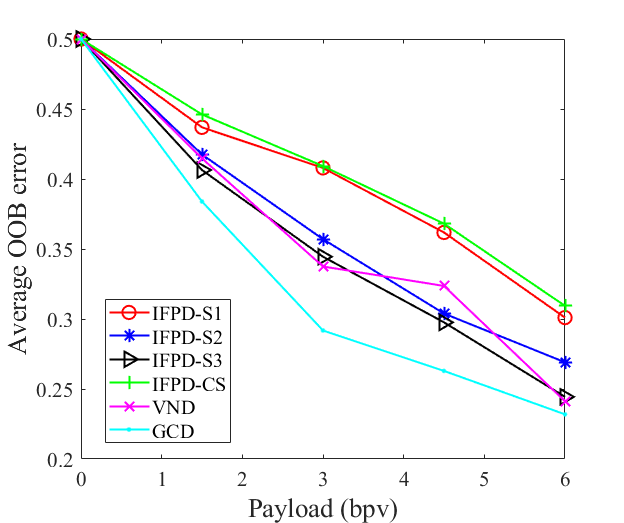
(a) PSB dataset

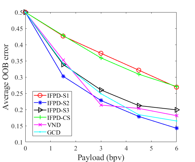
(b) PMN dataset

Figure 5: The varying trends of average $E_{OOB}$ of our algorithm w.r.t. different distortion functions, payloads ranging from 1 bpv to 6 bpv, and the PSB and PMN datasets. (a) Result for the PSB dataset. (b) Result for the PMN dataset.

4.2 Evaluation of FPD

4.2.1 Time Complexity of Distortion Calculation

By virtue of the analysis in Section 3.4 and Section 3.5, we know that sub-features $\phi_{65}\!\sim\!\phi_{76}$, $\phi_{77}\!\sim\!\phi_{88}$, and $\phi_{89}\!\sim\!\phi_{100}$ are the most suitable for FPD. However, it will be time-consuming if we directly adopt the original method in [14] to calculate $\rho(\delta_{i,j})$. Thus, we analyzed the three sub-features and proposed IFPD in Section 3.5. For simplicity, let OFPD-S1, OFPD-S2, OFPD-S3, and OFPD-CS denote four original cost calculation methods, where the first three are based on $\phi_{65}\!\sim\!\phi_{76}$, $\phi_{77}\!\sim\!\phi_{88}$, and $\phi_{89}\!\sim\!\phi_{100}$ respectively and the last one is a combined version of the first three. Accordingly, the improved methods are denoted by IFPD-S1, IFPD-S2, IFPD-S3, and IFPD-CS, respectively. To demonstrate the effectiveness of IFPD, we randomly selected some meshes from the PSB, PMN, and TSM datasets, and then calculated vertex-changing costs with different cost calculation methods when $\boldsymbol{I}=\{\frac{-6}{10^{k^{*}}},\cdots,\frac{-1}{10^{k^{*}}},0,\frac{1}{10^{k^{*}}},\cdots,\frac{6}{10^{k^{*}}}\}$. Table II lists the time consumption of each method on each mesh. From Table II, we can see that the OFPD-based methods are so time-consuming that processing meshes with more than 7000 vertices take more than one hour, but the usage of the IFPD series can remarkably speed up the cost calculation.

4.2.2 Evaluations of Different Distortion Profiles

To verify the validity of IFPD, we chose the vertex normal distortion (VND) and Gaussian curvature distortion (GCD), which were proposed in [22] for comparison. In [22], VND and GCD are defined respectively by

$$\begin{aligned} &VND(\boldsymbol{v}_{i})=\frac{1}{log(||\boldsymbol{n}_{\boldsymbol{v}_{i}}-\boldsymbol{n}_{SM(\boldsymbol{v}_{i})}||_{2}+1)+\sigma}\\ &GCD(\boldsymbol{v}_{i})=\frac{1}{K(\boldsymbol{v}_{i})^{\beta}+\sigma}\end{aligned},$$ (14)

where $\boldsymbol{n}_{\boldsymbol{v}_{i}}$ denotes the vertex normal of $\boldsymbol{v}_{i}$ and $\boldsymbol{n}_{SM(\boldsymbol{v}_{i})}$ is its smoothed version; $K(\boldsymbol{v}_{i})$ is the discrete Gaussian curvature of $\boldsymbol{v}_{i}$; $\sigma$ and $\beta$ are scalar parameters. Note that VND and GCD default that the non-zero elements in $\boldsymbol{I}$ have the same change cost. Four payloads 1.5, 3, 4.5, and 6 bpv are considered in the comparison experiments. Specifically, we set $\boldsymbol{I}=\{0,\frac{1}{10^{k^{*}}}\}$ for $\alpha=1.5$ bpv and adopted the 1-layered STC for message embedding. For $\alpha=3$ bpv, we limited $\boldsymbol{I}=\{\frac{-1}{10^{k^{*}}},0,\frac{1}{10^{k^{*}}},\frac{2}{10^{k^{*}}}\}$ and used 2-layered STC. $\boldsymbol{I}=\{\frac{-3}{10^{k^{*}}},\frac{-2}{10^{k^{*}}},\frac{-1}{10^{k^{*}}},0,\frac{1}{10^{k^{*}}},\frac{2}{10^{k^{*}}},\frac{3}{10^{k^{*}}},\frac{4}{10^{k^{*}}}\}$ and $\boldsymbol{I}=\{\frac{-7}{10^{k^{*}}},\cdots,\frac{-1}{10^{k^{*}}},0,\frac{1}{10^{k^{*}}},\cdots,\frac{7}{10^{k^{*}}},\frac{8}{10^{k^{*}}}\}$ were used respectively for payloads 4.5 and 6 bpv. Accordingly, 3-layered STC and 4-layered STC were adopted for the two payloads, respectively. We utilized the STC toolbox available on website¹ with the height of the submatrix $\widehat{\boldsymbol{\rm{H}}}_{l,j}$ set to 12. $k^{*}$ was set to 6 because, through our observation of these two datasets, we found that almost all vertex coordinates only keep six decimal places. Following the above settings, we conducted experiments using the PSB and PMN datasets. For the PSB dataset, 280 randomly-selected meshes and their stego counterparts were used as the training set, and the remaining 120 cover-stego pairs were used for testing. For the PMN dataset, we chose 1280 meshes for the experiments, 1000 cover-stego pairs as the training set and the rest as the test set. The division of the training and test sets on each dataset was repeated 30 times. We adopted a detector equipped with the FLD ensemble classifier [39] and 100-dimensional NVT+ features to evaluate these distortion functions. Furthermore, a separate classifier was trained for each distortion function and payload. The security was measured by the average $E_{OOB}$ over the 30 test sets. In addition, the form of normalization function in Eq. (6) is selectable, and in this work, it is given by

$$\frac{\rho(\delta_{i,j})-\rho_{min}}{\rho_{max}-\rho_{min}},\ \delta_{i,j}\in\boldsymbol{I},$$ (15)

where $\rho_{min}$ and $\rho_{max}$ represent the minimum and maximum values of $\{\rho(\delta_{i,j})\mid i\in\{1,\cdots,|\boldsymbol{V}|\},j\in\{x,y,z\}\}$ respectively. As shown in Fig. 5 (a), compared with VND and GCD, the steganographic algorithm using IFPD-S1 gains a notable improvement in security, and the progress becomes more significant as the payload increases. While IFPD-S2, IFPD-S3, and VND perform comparably, the combination version IFPD-CS outperforms VND and GCD remarkably, demonstrating the effectiveness of IFPD on the PSB dataset. As for Fig. 5 (b), IFPD-S1 also boosts the steganographic security significantly, but its average $E_{OOB}$ w.r.t. different payloads are lower than those on the PSB dataset. This is because, as described in [14], NVT+ steganalyzer can achieve better detection performance on the PMN dataset than on the PSB dataset. It is worth noting that IFPD-S1, IFPD-S2, and IFPD-S3 perform pretty differently on both datasets, with IFPD-S1 exhibiting an absolute advantage in anti-steganalysis and the performance of the other two similar to that of VND and GCD. This suggests that IFPD with sub-features that are effective for steganalysis does not necessarily improve the security of our algorithm significantly. In addition, the performance similarity of IFPD-S1 and IFPD-CS implies that preserving more features may not be as effective as we think. Despite all this, to avoid overfitting to a particular steganalyzer as much as possible [17], we still chose IFPD-CS as the distortion function for the following experiments.

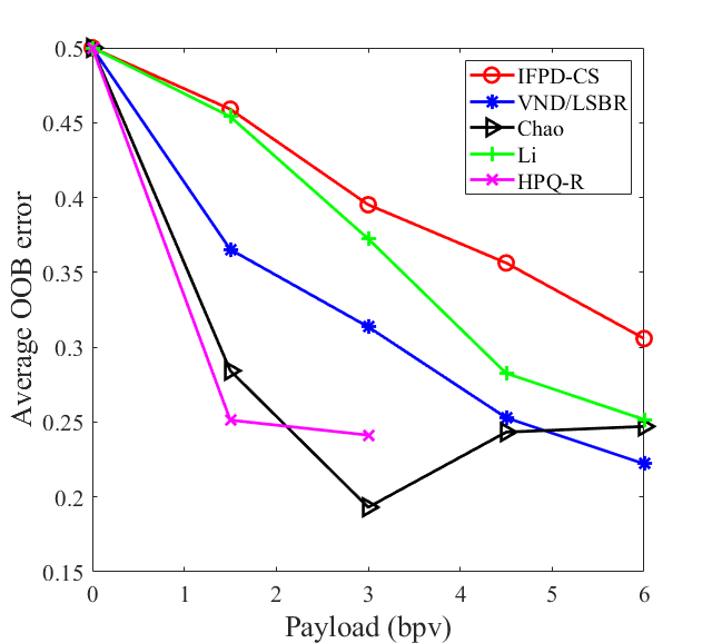
(a) LFS52, PSB dataset

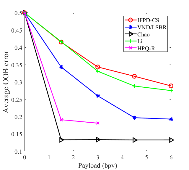
(b) LFS52, PMN dataset

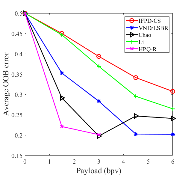
(c) LFS64, PSB dataset

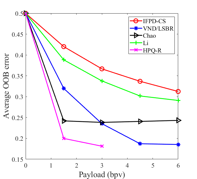
(d) LFS64, PMN dataset

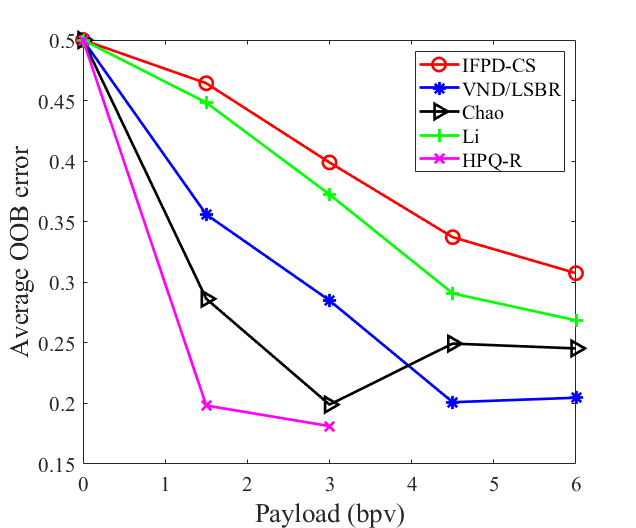
(e) LFS76, PSB dataset

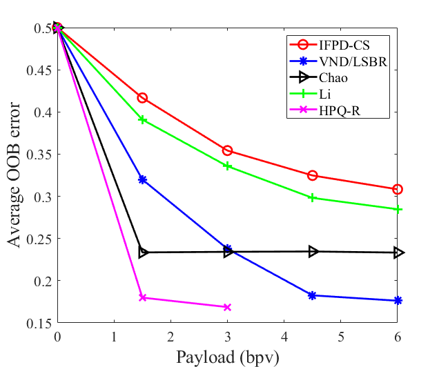
(f) LFS76, PMN dataset

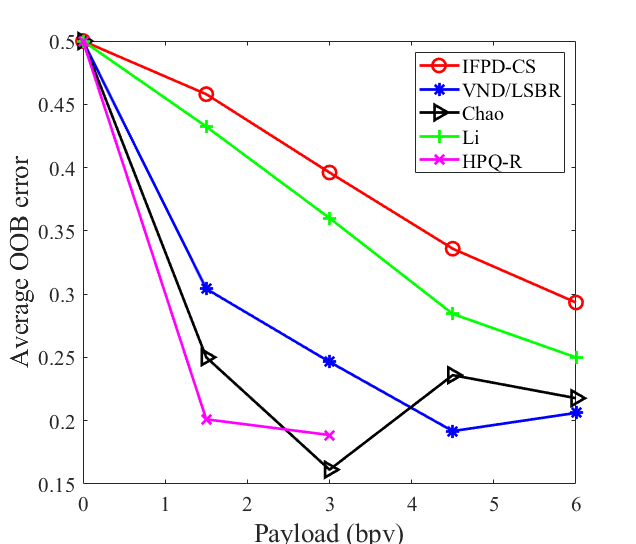
(g) ELFS124, PSB dataset

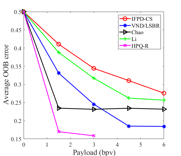
(h) ELFS124, PMN dataset

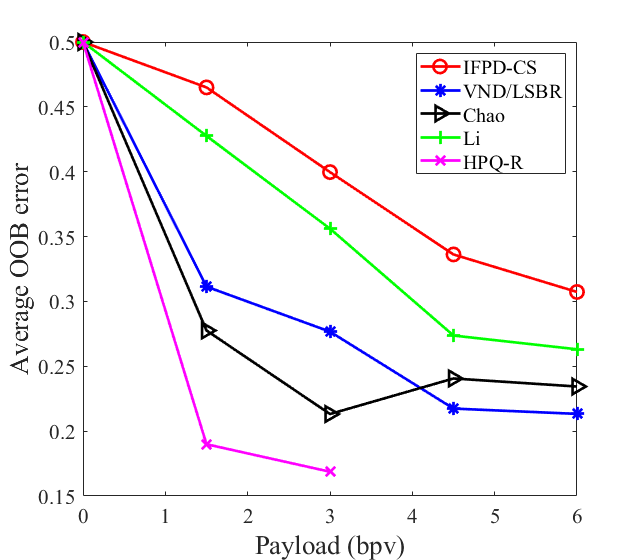
(i) WFS228, PSB dataset

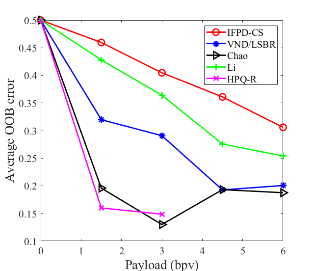
(j) NVT+, PSB dataset

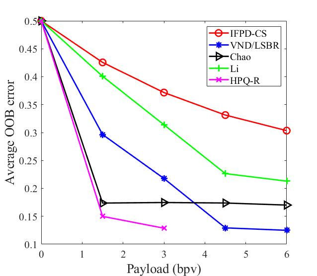
(k) NVT+, PMN dataset

Figure 6: The varying trends of the average $E_{OOB}$ of IFPD-CS, Chao, Li, VND/LSBR, and HPQ-R w.r.t different payloads, 3D steganalyzers, and datasets.

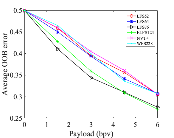
(a) PSB dataset

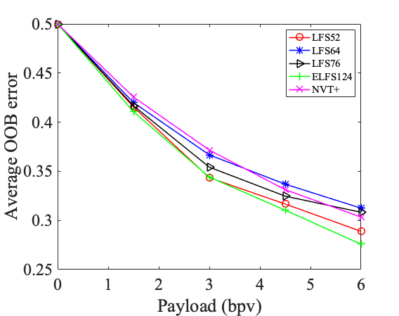
(b) PMN dataset

Figure 7: The varying trends of average $E_{OOB}$ of IFPD-CS tested under different 3D steganalyzers w.r.t. payloads ranging from 0 bpv to 6 bpv. (a) Result for the PSB dataset. (b) Result for the PMN dataset.

TABLE III: P-values of IFPD-CS on the PSB dataset w.r.t Chao, Li, VND/LSBR, and HPQ-R under different payloads and 3D steganalyzers.

		Chao	Li	VND/LSBR	HPQ-R
LFS52	$\alpha=1.5$	$8.4556\times 10^{-18}$	0.9998	$8.4556\times 10^{-18}$	$8.4556\times 10^{-18}$
	$\alpha=3$	$8.4556\times 10^{-18}$	$2.1724\times 10^{-10}$	$8.4556\times 10^{-18}$	$8.4556\times 10^{-18}$
	$\alpha=4.5$	$8.4556\times 10^{-18}$	$5.5283\times 10^{-14}$	$8.4556\times 10^{-18}$	-
	$\alpha=6$	$8.4556\times 10^{-18}$	$3.4600\times 10^{-12}$	$8.4556\times 10^{-18}$	-
LFS64	$\alpha=1.5$	$8.4556\times 10^{-18}$	0.0766	$8.4556\times 10^{-18}$	$8.4556\times 10^{-18}$
	$\alpha=3$	$8.4556\times 10^{-18}$	$1.4271\times 10^{-8}$	$8.4556\times 10^{-18}$	$8.4556\times 10^{-18}$
	$\alpha=4.5$	$8.4556\times 10^{-18}$	$9.7805\times 10^{-12}$	$8.4556\times 10^{-18}$	-
	$\alpha=6$	$8.4556\times 10^{-18}$	$1.2880\times 10^{-8}$	$8.4556\times 10^{-18}$	-
LFS76	$\alpha=1.5$	$8.4556\times 10^{-18}$	0.7130	$8.4556\times 10^{-18}$	$8.4556\times 10^{-18}$
	$\alpha=3$	$8.4556\times 10^{-18}$	$3.0429\times 10^{-5}$	$8.4556\times 10^{-18}$	$8.4556\times 10^{-18}$
	$\alpha=4.5$	$8.4556\times 10^{-18}$	$4.1049\times 10^{-13}$	$8.4556\times 10^{-18}$	-
	$\alpha=6$	$8.4556\times 10^{-18}$	$5.7485\times 10^{-11}$	$8.4556\times 10^{-18}$	-
ELFS124	$\alpha=1.5$	$8.4556\times 10^{-18}$	$2.0954\times 10^{-6}$	$8.4556\times 10^{-18}$	$8.4556\times 10^{-18}$
	$\alpha=3$	$8.4556\times 10^{-18}$	0.0036	$8.4556\times 10^{-18}$	$8.4556\times 10^{-18}$
	$\alpha=4.5$	$8.4556\times 10^{-18}$	$1.6684\times 10^{-9}$	$8.4556\times 10^{-18}$	-
	$\alpha=6$	$8.4556\times 10^{-18}$	$6.7545\times 10^{-6}$	$8.4556\times 10^{-18}$	-
NVT+	$\alpha=1.5$	$8.4556\times 10^{-18}$	$2.1823\times 10^{-8}$	$8.4556\times 10^{-18}$	$8.4556\times 10^{-18}$
	$\alpha=3$	$8.4556\times 10^{-18}$	$1.8789\times 10^{-11}$	$8.4556\times 10^{-18}$	$8.4556\times 10^{-18}$
	$\alpha=4.5$	$8.4556\times 10^{-18}$	$2.5367\times 10^{-17}$	$8.4556\times 10^{-18}$	-
	$\alpha=6$	$8.4556\times 10^{-18}$	$1.0705\times 10^{-14}$	$8.4556\times 10^{-18}$	-
WFS228	$\alpha=1.5$	$8.4556\times 10^{-18}$	$1.7130\times 10^{-13}$	$8.4556\times 10^{-18}$	$8.4556\times 10^{-18}$
	$\alpha=3$	$8.4556\times 10^{-18}$	$3.8482\times 10^{-10}$	$8.4556\times 10^{-18}$	$8.4556\times 10^{-18}$
	$\alpha=4.5$	$8.4556\times 10^{-18}$	$1.5220\times 10^{-16}$	$8.4556\times 10^{-18}$	-
	$\alpha=6$	$8.4556\times 10^{-18}$	$1.1112\times 10^{-13}$	$8.4556\times 10^{-18}$	-

TABLE IV: P-values obtained by IFPD-CS on the PMN dataset w.r.t Chao, Li, VND/LSBR, and HPQ-R under different payloads and 3D steganalyzers.

		Chao	Li	VND/LSBR	HPQ-R
LFS52	$\alpha=1.5$	$8.4556\times 10^{-18}$	1.000	$8.4556\times 10^{-18}$	$8.4556\times 10^{-18}$
	$\alpha=3$	$8.4556\times 10^{-18}$	$0.0062$	$8.4556\times 10^{-18}$	$8.4556\times 10^{-18}$
	$\alpha=4.5$	$8.4556\times 10^{-18}$	$7.7620\times 10^{-10}$	$8.4556\times 10^{-18}$	-
	$\alpha=6$	$8.4556\times 10^{-18}$	0.0892	$8.4556\times 10^{-18}$	-
LFS64	$\alpha=1.5$	$8.4556\times 10^{-18}$	$9.1907\times 10^{-9}$	$8.4556\times 10^{-18}$	$8.4556\times 10^{-18}$
	$\alpha=3$	$8.4556\times 10^{-18}$	$4.2714\times 10^{-7}$	$8.4556\times 10^{-18}$	$8.4556\times 10^{-18}$
	$\alpha=4.5$	$8.4556\times 10^{-18}$	$3.5312\times 10^{-9}$	$8.4556\times 10^{-18}$	-
	$\alpha=6$	$8.4556\times 10^{-18}$	$1.1071\times 10^{-4}$	$8.4556\times 10^{-18}$	-
LFS76	$\alpha=1.5$	$8.4556\times 10^{-18}$	$1.6945\times 10^{-12}$	$8.4556\times 10^{-18}$	$8.4556\times 10^{-18}$
	$\alpha=3$	$8.4556\times 10^{-18}$	$1.6383\times 10^{-8}$	$8.4556\times 10^{-18}$	$8.4556\times 10^{-18}$
	$\alpha=4.5$	$8.4556\times 10^{-18}$	$2.5367\times 10^{-17}$	$8.4556\times 10^{-18}$	-
	$\alpha=6$	$8.4556\times 10^{-18}$	$2.8411\times 10^{-15}$	$8.4556\times 10^{-18}$	-
ELFS124	$\alpha=1.5$	$8.4556\times 10^{-18}$	$3.2652\times 10^{-5}$	$8.4556\times 10^{-18}$	$8.4556\times 10^{-18}$
	$\alpha=3$	$8.4556\times 10^{-18}$	$6.5049\times 10^{-9}$	$8.4556\times 10^{-18}$	$8.4556\times 10^{-18}$
	$\alpha=4.5$	$8.4556\times 10^{-18}$	$8.4556\times 10^{-18}$	$8.4556\times 10^{-18}$	-
	$\alpha=6$	$8.4556\times 10^{-18}$	$1.6820\times 10^{-10}$	$8.4556\times 10^{-18}$	-
NVT+	$\alpha=1.5$	$8.4556\times 10^{-18}$	$6.9277\times 10^{-14}$	$8.4556\times 10^{-18}$	$8.4556\times 10^{-18}$
	$\alpha=3$	$8.4556\times 10^{-18}$	$8.4556\times 10^{-18}$	$8.4556\times 10^{-18}$	$8.4556\times 10^{-18}$
	$\alpha=4.5$	$8.4556\times 10^{-18}$	$8.4556\times 10^{-18}$	$8.4556\times 10^{-18}$	-
	$\alpha=6$	$8.4556\times 10^{-18}$	$8.4556\times 10^{-18}$	$8.4556\times 10^{-18}$	-

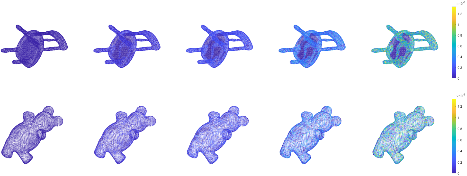
(a) PSB

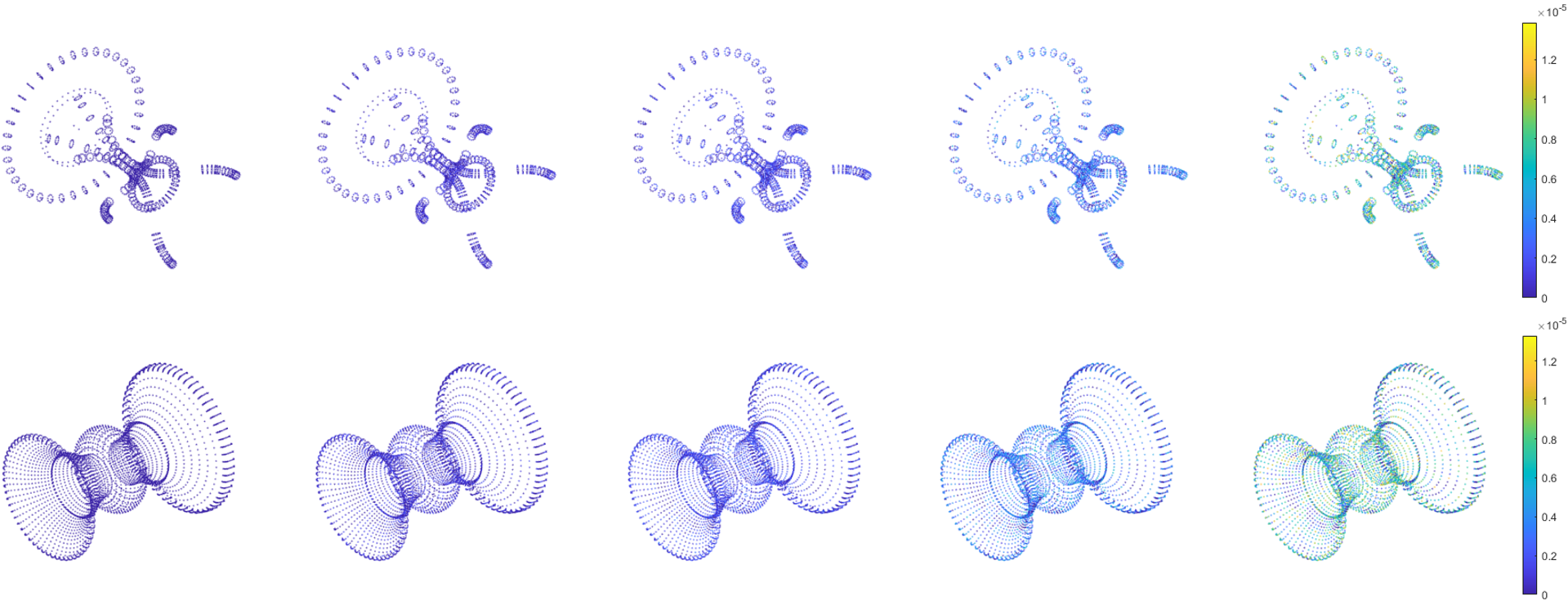
(b) PMN

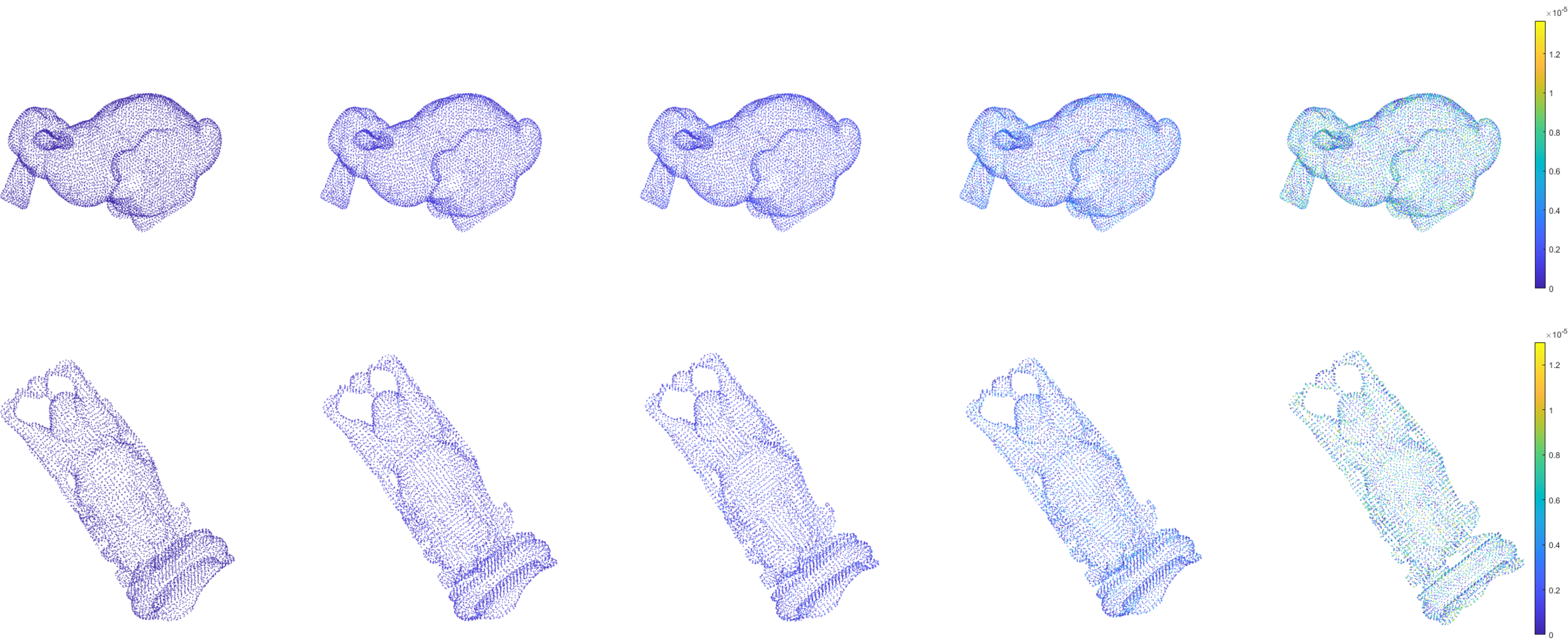
(c) TSM

Figure 8: Embedding visualization results of “chair”, “bear”, “round table”, “vase”, “bunny”, and “buddha” from the PSB, PMN, and TSM datasets. Visualization examples in each row correspond to the stego meshes embedded with payloads 0, 1.5, 3, 4.5, and 6 bpv, respectively.

4.3 Comparison to State-of-the-Art Algorithms

To verify the effectiveness of our algorithm, we chose four 3D mesh steganographic algorithms based on geometric modification, namely VND/LSBR [22], Chao [6], Li [8], and HPQ-R [16], for comparison. All these algorithms provide high embedding capacity, and besides, VND/LSBR and HPQ-R can potentially resist 3D steganalysis. Relevant experiments were carried out on the PSB and PMN datasets with payloads 1.5, 3, 4.5, and 6 bpv. The division of the training and test sets is consistent with that described in Section 4.2.2. Since the vertex coordinates of almost all meshes in PSB and PMN are accurate to at most six decimal places, we made the following settings for each algorithm to ensure that the embedding operations would not cause the vertices to change beyond this precision. For Chao, we set the interval number and the maximum number of embedding layers to 100000 and 2, respectively. For VND/LSBR, we set the starting layer of the adaptive embedding to be layer 14 and the following two layers to be used for LSBR embedding. As for Li, we fixed the truncated space size of each vertex to 1. The interval parameter of HPQ-R was set to $10^{-5}$, and the number of sub-intervals was set to $2^{3}$. Note that we did not consider HPQ-R at high payloads, namely 4.5 and 6 bpv, because a higher payload needs a larger sub-interval number, which causes vertices to change beyond the allowed precision. The embedding strategy used by our algorithm for different payloads is the same as described in the previous section. Furthermore, six steganalyzers based on LFS52, LFS64, LFS76, ELFS124, WFS228, and NVT+ were used to evaluate steganographic security. The security of each algorithm w.r.t. different payloads was measured by the average $E_{OOB}$ overall 30 trials. For simplicity, we refer to these steganalyzers by their respective feature set names. Please note that we did not conduct relevant experiments of WFS228 on PMN because WFS228’s source code, which is available on the website , fails to run for most meshes in this dataset. The experimental results are reported from Fig. 6 (a) to Fig. 6 (k). As illustrated in the eleven subfigures of Fig. 6, IFPD-CS achieves better anti-steganalysis performance than the other four on both PSB and PMN except for Li at low payloads, which may be because the number of vertices changed by Li is minimal when the payload is low. However, as the payload increases, the security of Li declines progressively, and the superiority of IFPD-CS is gradually revealed.

We also show the average $E_{OOB}$ of IFPD-CS at payloads ranging from 0 bpv to 6 bpv w.r.t. various 3D steganalyzers in Fig. 7. According to the experimental results shown in [14] and [25], we know the steganalysis performance of NVT+ is outstanding relative to other steganalyzers. However, Fig. 7 (a) and 7 (b) consistently exhibit an experimental phenomenon that the ability of NVT+ to detect IFPD-CS is rather mediocre on both datasets. This directly reflects that IFPD-CS indeed preserves some NVT+ steganalysis features so that NVT+ with eye-catching detection performance becomes less impressive. Besides, this phenomenon also exposes a practical issue that the current 3D steganalytic features are not universal enough.

4.4 Statistical Significance Test

Given that the test error rate distribution of Chao, Li, VND/LSBR, IFPD-CS, and HPQ-R is unknown, we adopted the Wilcoxon rank sum test to evaluate the statistical significance of the security enhancement brought by IFPD-CS w.r.t. the other four algorithms under different payloads, steganalyzers, and datasets. The hypothesis test was constructed as follows.

$$H_{0}:\mu_{1}=\mu_{2},H_{1}:\mu_{1}>\mu_{2},$$ (16)

where $\mu_{1}$ is the mean values of $n_{1}$ test error rates of IFPD-CS; $\mu_{2}$ is the mean values of $n_{2}$ test error rates of the comparison algorithm. In this case, we set $n_{1}=n_{2}=30$. $\mu_{1}=\mu_{2}$ indicates there is no significant difference between them. Let $R$ denote the rank sum of IFPD-CS test error rate samples. Since $n_{1},n_{2}\geq 10$, $R\sim N(\mu_{R},\sigma_{R}^{2})$ where $\mu_{R}=\frac{n_{1}(n_{1}+n_{2}+1)}{2}$ and $\sigma^{2}_{R}=\frac{n_{1}n_{2}(n_{1}+n_{2}+1)}{12}$. Therefore, we can use

$$Z=\frac{R-\mu_{R}}{\sigma_{R}}$$ (17)

as the test statistic. We calculated the value of $Z$ and obtained the corresponding p-value through the built-in function $ranksum$ of Matlab. The significant level was set to 0.05. If the p-value is less than the significant level, the null hypothesis $H_{0}$ will be rejected; otherwise, we can deem the improvement of IFPD-CS in steganographic security statistically significant and reliable. Relevant experimental results on the PSB and PMN datasets are presented in Table III and Table IV respectively, where p-values greater than the significance level are represented in bold. In a nutshell, compared with Chao, VND/LSBR, and HPD-R, IFPD-CS has a remarkable security enhancement, but for Li at low payloads, the enhancement is not always significant, which is consistent with the experimental results shown in Fig. 6.

4.5 Visualization of Message Embedding

To more intuitively express the embedding impact brought by our algorithm, we measured the change degree of each vertex by the root-mean-square error and visualized it with colors ranging from blue to yellow. Fig. 8 shows the embedding visualization results of several meshes from the PSB, PMN, and TSM datasets. Specifically, visualization examples in each row correspond to the stego meshes under payloads 0, 1.5, 3, 4.5, and 6 bpv, respectively. Note that we do not show the mesh edges because our algorithm does not change the topology of meshes. From Fig. 8, we can see that for low payloads, the distortion caused by our algorithm to meshes is imperceptible, showing that our algorithm can preserve some local and global geometric features of meshes, such as sharp features, to a great extent.

4.6 Analysis of Computational Complexity

According to Section 3.6, we know the message embedding procedure consists of two parts, namely calculation of $\rho(\delta_{i,j})$ for all vertices and $\delta_{i,j}\in\boldsymbol{I}$ and $Q$-layered STC. For the former, without losing generality, let $t$ denote the calculational complexity of $\rho(\delta_{i,j})$. Given a mesh with $|\boldsymbol{V}|$ vertices, when $\boldsymbol{I}$ is determined, we can easily get the costing complexity of the mesh as $O(t|\boldsymbol{V}||\boldsymbol{I}|)$. Distinctly, cost function design, vertex number, and $\boldsymbol{I}$ are three crucial factors affecting the time consumption of the first part. IFPD proposed in Section 3.5 greatly reduces $t$, and the results shown in Table II further demonstrate that the IFPD series can speed up the calculation of $\rho(\delta_{i,j})$, which enhances the practicality of our algorithm. As for the second part, thanks to the efficient steganographic coding technique $Q$-layered STC, the time consumption of the practical message embedding can be ignored when compared with that of the first part. Please refer to [24] for more details on the computational complexity of STC.

4.7 Robustness Analysis

In traditional steganography, scholars are more concerned with steganographic security than robustness. However, in order to move steganography from the laboratory into the real world, a discussion on the robustness of steganography is essential. Zhou et al. [25] enumerated several specific attacks targetting 3D mesh steganography, i.e., affine transformation, vertex reordering, smoothing, simplification, and noise addition. We admit our algorithm is not robust enough against geometric attacks, such as affine transformation and noise addition, but can effectively resist permutation attacks, such as vertex reordering. This is principally because our algorithm is based on vertex modification, and geometric attacks inevitably cause vertex coordinates to change, tremendously reducing the success rate of the message retrieval of our algorithm without using any error correction code.

5 Conclusion

In this paper, we proposed a highly adaptive 3D mesh steganographic algorithm based on FPD. The innovation of our work is embodied in the PLS problem construction, embedding domain construction, distortion function design and improvement, and universal and automatic BMP calculation approach for $Q$-layered STC. Extensive experiments in Section 4 demonstrate the superiority of our algorithm in security.

In fact, the research on 3D steganography has been sidelined for a long time. However, with the rapid advance of 3D technology, 3D models will become increasingly popular in our daily life, and hence, we firmly believe that 3D steganography has a bright prospect. At present, there are still many topics worth studying in 3D steganography. For example, as we know, the distortion function plays a pivotal role in adaptive steganography. A well-designed distortion function can dramatically boost the security of steganography. The experimental results shown in Fig. 7 inevitably raise concerns that the proposed FPD may overfit some particular steganalyzers. Therefore, how to design a more general distortion model is the focus of our future research. Besides, as analyzed in Section 4.7, our algorithm has poor robustness against geometric attacks. To move 3D steganography from the laboratory to real life, the robustness of 3D steganography is worth further discussion and study.

Appendix A Analysis of NVT+ Sub-features

Table V provides the geometric feature relevant to each sub-feature of NVT+.

Test details. We selected 380 mesh models from the PSB and PMN datasets apiece. For the meshes from each dataset, we used LSBM ($\pm 1$), Chao [6], VND/LSBR [22], and Li [8] to generate their stego counterparts, and finally obtained four mesh sets, each of which contains 380 pairs of cover and stego meshes. For each set, we randomly selected 260 pairs for training and the rest for testing, and such division of the training and test sets was repeated 30 times. Then, we adopted the FLD ensemble [39] as the classifier due to its reliable detection accuracy and fast training. We set the payload $\alpha=3$ bpv for the four algorithms. The ultimate steganographic security was quantified by the average $E_{OOB}$ over 30 trials. The average $E_{OOB}$ of each sub-feature is shown in Fig. 9. The dotted lines in Fig. 9, derived from polynomials of order 6, show the varying trends of the average $E_{OOB}$ w.r.t. NVT+ sub-features for different steganographic algorithms.

Findings. From Fig. 9 (a), we can see that the trendlines of the four algorithms reach their troughs consistently around the sub-feature $\phi_{33}\sim\phi_{36}$, and then plummet together near the sub-feature $\phi_{65}\sim\phi_{64}$, indicating that sub-features $\phi_{33}\sim\phi_{36}$, $\phi_{65}\sim\phi_{76}$, $\phi_{77}\sim\phi_{88}$, and $\phi_{89}\sim\phi_{100}$ are relatively effective for steganalysis on the PSB dataset. For the PMN dataset, $\phi_{33}\sim\phi_{36}$ loses its effectiveness, but the precipitous fall occurs again near $\phi_{65}\sim\phi_{76}$, showing that the last three sub-features are still effective in detecting the steganographic algorithms. In addition, it is a wonder that the sub-feature $\phi_{1}\sim\phi_{12}$, which is useless for steganalysis on the PSB dataset, bounces back on the PMN dataset.

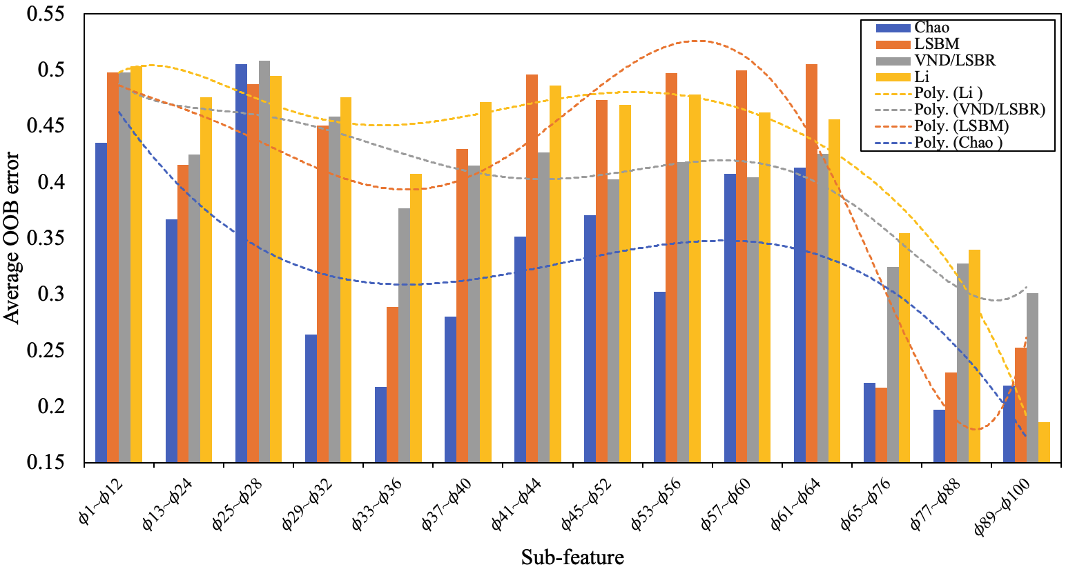
(a) PSB dataset

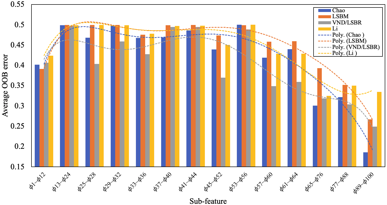
(b) PMN dataset

Figure 9: The average $E_{OOB}$ of NVT+ sub-features w.r.t. LSBM, VND/LSBR, Chao, and Li under $\alpha$ = 3 bpv. Each dotted line in the two figures describes the varying trend of the average $E_{OOB}$ of the corresponding algorithm w.r.t. different NVT+ sub-features. (a) PSB dataset tested under NVT+ sub-features. (b) PMN dataset tested under NVT+ sub-features.

TABLE V: Brief review of the sub-features of NVT+ in this paper.

Sub-feature	Relevant geometric feature
$\phi_{1}\sim\phi_{12}$	Vertex coordinates in the Cartesian coordinate system.
$\phi_{13}\sim\phi_{24}$	Vertex coordinates in the Laplacian coordinate system.
$\phi_{25}\sim\phi_{28}$	$l_{2}$-norm of vertices in the Cartesian coordinate system.
$\phi_{29}\sim\phi_{32}$	$l_{2}$-norm of vertices in the Laplacian coordinate system.
$\phi_{33}\sim\phi_{36}$	Dihedral angle.
$\phi_{37}\sim\phi_{40}$	Face normal.
$\phi_{41}\sim\phi_{44}$	Vertex normal.
$\phi_{45}\sim\phi_{52}$	Gaussian curvature and curvature ratio.
$\phi_{53}\sim\phi_{56}$	Edge normal.
$\phi_{57}\sim\phi_{60}$	Mean curvature.
$\phi_{61}\sim\phi_{64}$	Total curvature.
$\phi_{65}\sim\phi_{76}$	Normal voting tensors based on $\mathcal{N}_{1}$ (See Fig. 3 (a)).
$\phi_{77}\sim\phi_{88}$	Normal voting tensors based on $\mathcal{N}_{2}$ (See Fig. 3 (b)).
$\phi_{89}\sim\phi_{100}$	Normal voting tensors based on $\mathcal{N}_{3}$ (See Fig. 3 (c)).

References

- [1] J. Fridrich, Steganography in Digital Media: Principles, Algorithms, and Applications. Cambridge, U.K.: Cambridge Univ. Press, 2009.
- [2] C. R. Qi, H. Su, K. Mo, and L. J. Guibas, “Pointnet: Deep learning on point sets for 3D classification and segmentation,” in Proc. IEEE Conf. Comput. Vision Pattern Recogni., Honolulu, HI, USA, 2017, pp. 77–85.
- [3] F. Cayre and B. Macq, “Data hiding on 3-D triangle meshes,” IEEE Trans. Signal Process., vol. 51, no. 4, pp. 939–949, Apr. 2003.
- [4] C.-M. Wang and Y.-M. Cheng, “An efficient information hiding algorithm for polygon models,” Comput. Graph. Forum, vol. 24, no. 3, pp. 591–600, Sep. 2005.
- [5] Y.-M. Cheng and C.-M. Wang, “A high-capacity steganographic approach for 3D polygonal meshes,” Visual Comput., vol. 22, no. 9-11, pp. 845–855, Sep. 2006.
- [6] M.-W. Chao, C.-H. Lin, C.-W. Yu, and T.-Y. Lee, “A high capacity 3D steganography algorithm,” IEEE Trans. Vis. Comput. Graph., vol. 15, no. 2, pp. 274–84, Mar. 2009.
- [7] V. Itier and W. Puech, “High capacity data hiding for 3D point clouds based on static arithmetic coding,” Multimed. Tools Appl., vol. 76, no. 24, pp. 1–25, Dec. 2017.
- [8] N. Li, J. Hu, R. Sun, S. Wang, and Z. Luo, “A high-capacity 3D steganography algorithm with adjustable distortion,” IEEE Access, vol. 5, pp. 24 457–24 466, 2017.
- [9] Y. Yang and I. Ivrissimtzis, “Mesh discriminative features for 3D steganalysis,” ACM Trans. Multimed. Comput. Commun. Appl., vol. 10, no. 3, p. 27, Apr. 2014.
- [10] Z. Li and A. G. Bors, “3D mesh steganalysis using local shape features,” in Proc. IEEE Int. Conf. Acoust. Speech Signal Process., Barcelona, Spain, 2016, pp. 2144–2148.
- [11] D. Kim, H.-U. Jang, H.-Y. Choi, J. Son, I.-J. Yu, and H.-K. Lee, “Improved 3D mesh steganalysis using homogeneous kernel map,” in Proc. Int. Conf. inf. Sci. Appl., Macau, China, 2017, pp. 358 – 365.
- [12] Z. Li and A. G. Bors, “Steganalysis of 3D objects using statistics of local feature sets,” Inf. Sci., vol. 415-416, pp. 85–99, Nov. 2017.
- [13] Z. Li, D. Gong, F. Liu, and A. G. Bors, “3D steganalysis using the extended local feature set,” in Proc. IEEE Int. Conf. Image Process., Athens, Greece, 2018, pp. 1683–1687.
- [14] H. Zhou, K. Chen, W. Zhang, C. Qin, and N. Yu, “Feature-preserving tensor voting model for mesh steganalysis,” IEEE Trans. Vis. Comput. Graph., vol. 27, no. 1, pp. 57–67, Jan. 2021.
- [15] Z. Li and A. G. Bors, “Steganalysis of meshes based on 3D wavelet multiresolution analysis,” Inf. Sci., vol. 522, pp. 164–179, 2020.
- [16] Z. Li, S. Beugnon, W. Puech, and A. G. Bors, “Rethinking the high capacity 3D steganography: Increasing its resistance to steganalysis,” in Proc. IEEE Int. Conf. Image Process., Beijing, China, 2017, pp. 510–414.
- [17] T. Pevný, T. Filler, and P. Bas, “Using high-dimensional image models to perform highly undetectable steganography,” in Proc. 12th Int. Workshop Information Hiding, Calgary, Canada, 2010.
- [18] V. Holub and J. Fridrich, “Designing steganographic distortion using directional filters,” in Proc. IEEE Int. Workshop Inf. Forensics Security, Tenerife, Spain, 2012, pp. 234–239.
- [19] V. Holub, J. Fridrich, and T. Denemark, “Universal distortion function for steganography in an arbitrary domain,” Eurasip J. Inf. Secur., vol. 2014, no. 1, p. 1–13, Jan. 2014.
- [20] L. Guo, J. Ni, and Y. Shi, “Uniform embedding for efficient jpeg steganography,” IEEE Trans. Inf. Forensic Secur., vol. 9, no. 5, pp. 814–825, May 2014.
- [21] L. Guo, J. Ni, W. Su, C. Tang, and Y. Shi, “Using statistical image model for jpeg steganography: Uniform embedding revisited,” IEEE Trans. Inf. Forensic Secur., vol. 10, no. 12, pp. 2669–2680, Dec. 2015.
- [22] H. Zhou, K. Chen, W. Zhang, Y. Yao, and N. Yu, “Distortion design for secure adaptive 3-D mesh steganography,” IEEE Trans. Multimedia, vol. 21, no. 6, pp. 1384–1398, Jun. 2019.
- [23] T. Filler and J. Fridrich, “Gibbs construction in steganography,” IEEE Trans. Inf. Forensic Secur., vol. 5, no. 4, pp. 705–720, Jan. 2010.
- [24] T. Filler, J. Judas, and J. Fridrich, “Minimizing additive distortion in steganography using syndrome-trellis codes,” IEEE Trans. Inf. Forensic Secur., vol. 6, no. 3, pp. 920–935, Oct. 2011.
- [25] H. Zhou, W. Zhang, K. Chen, W. Li, and N. Yu, “Three-dimensional mesh steganography and steganalysis: A review,” IEEE Trans. Vis. Comput. Gr., to be published, doi: 10.1109/TVCG.2021.3075136.
- [26] Y. Yang, N. Peyerimhoff, and I. Ivrissimtzis, “Linear correlations between spatial and normal noise in triangle meshes,” IEEE Trans. Vis. Comput. Graph., vol. 19, no. 1, pp. 45–55, Jan. 2013.
- [27] A. Bogomjakov, C. Gotsman, and M. Isenburg, “Distortion‐free steganography for polygonal meshes,” Comput. Graph. Forum, vol. 27, no. 2, pp. 637–642, Apr. 2008.
- [28] N.-C. Huang, M.-T. Li, and C.-M. Wang, “Toward optimal embedding capacity for permutation steganography,” IEEE Signal Process. Lett., vol. 16, no. 9, pp. 802–805, Oct. 2009.
- [29] S.-C. Tu, W.-K. Tai, M. Isenburg, and C.-C. Chang, “An improved data hiding approach for polygon meshes,” Visual Comput., vol. 26, no. 9, pp. 1177–1181, Sep. 2010.
- [30] S. Tu, H. Hsu, and W. Tai, “Permutation steganography for polygonal meshes based on coding tree,” Int. J. Virtual Real., vol. 9, no. 4, pp. 55–60, Nov. 2010.
- [31] S.-C. Tu and W.-K. Tai, “A high-capacity data-hiding approach for polygonal meshes using maximum expected level tree,” Comput. Graph., vol. 36, no. 6, p. 767–775, Oct. 2012.
- [32] N. Aspert, E. Gelasca, Y. Maret, and T. Ebrahimi, “Steganography for three-dimensional polygonal meshes,” in Proc. SPIE Int. Soc. Opt. Eng., Seattle, WA, US, 2002, vol. 4790, pp. 211–219.
- [33] M. G. Wagner, “Robust watermarking of polygonal meshes,” in Proc. Geom. Model. Process.: Theory Appl., Hong Kong, China, 2000, pp. 201–208.
- [34] Y. Maret and T. Ebrahimi, “Data hiding on 3D polygonal meshes,” in Proc. Multimed. Secur. Workshop, Magdeburg, Germany, 2004, pp. 68–74.
- [35] H. Kaveh and M.-S. Moin, “A high-capacity and low-distortion 3D polygonal mesh steganography using surfacelet transform,” Secur. Commun. Netw., vol. 8, no. 2, pp. 159–167, Jan. 2015.
- [36] J. Fridrich, M. Goljan, and D. Hogea, “Steganalysis of jpeg images: Breaking the f5 algorithm,” in Information Hiding, 5th Int. Workshop, ser. Lecture Notes Comput. Sci., Noordwikkerhout, Netherlands, 2002, pp. 310–323.
- [37] J. Kodovsky, S. Binghamton, and J. Fridrich, “Calibration revisited,” in Proc. ACM Multimedia Secur. Workshop, Princeton, NJ, USA, 2009.
- [38] Z. Li and A. G. Bors, “Selection of robust and relevant features for 3-d steganalysis,” IEEE Trans. Cybern., vol. 50, no. 5, pp. 1989–2001, May 2020.
- [39] J. Kodovsky, J. Fridrich, and V. Holub, “Ensemble classifiers for steganalysis of digital media,” IEEE Trans. Inf. Forensics Secur., vol. 7, no. 2, pp. 432–444, Apr. 2012.
- [40] Y. Wang, L. Kong, Z. Qian, G. Feng, X. Zhang, and J. Zheng, “Breaking permutation-based mesh steganography and security improvement,” IEEE Access, vol. 7, pp. 183 300–183 310, 2019.
- [41] R. Jiang, H. Zhou, W. Zhang, and N. Yu, “Reversible data hiding in encrypted three-dimensional mesh models,” IEEE Trans. Multimedia, vol. 20, no. 1, pp. 55–67, Jan. 2018.