Monogenic Signal Associated with Linear Canonical Transform and Application to Edge Detection Problems

Abstract

Monogenic signal is regarded as a generalization of analytic signal from the one dimensional space to the high dimensional space. It is defined by an original signal with the combination of Riesz transform. Then it provides the signal features representation, such as the local attenuation and the local phase vector. The main objective of this study is to analyze the local phase vector and the local attenuation in the high dimensional spaces. The differential phase congruency is applied for the edge detection problems.

Keywords:  Monogenic signal, Linear canonical transform, Edge detection

Mathematics Subject Classification (2010):  15A67, 42B10, 30G35

1 Analytic signal associated with LCT in one dimensional case

Let $\{a,b,c,d\}$ be real parameters satisfying $ad-bc=1$. The linear canonical transform (LCT) [1, 2] of the integrable signal $f$ is defined by

$$F^{(a,b,c,d)}(\omega)=\mathscr{L}^{(a,b,c,d)}(f)(\omega):=\begin{cases}\int_{\mathbf{R}}\mathcal{K}^{(a,b,c,d)}(\omega,x)f(x)dx,&b\neq 0;\\ \sqrt{d}e^{\frac{\mathbf{i}cd}{2}\omega^{2}}f(d\omega),&b=0;\end{cases}$$

where

$$\mathcal{K}^{(a,b,c,d)}(\omega,x):=\frac{1}{\sqrt{\mathbf{i}2\pi b}}e^{\mathbf{i}(\frac{d}{2b}\omega^{2}-\frac{1}{b}\omega x+\frac{a}{2b}x^{2})}.$$

Note that when $b=0$, the LCT is just a chirp multiplication. Given the similarity between the $b>0$ case and and $b<0$ case, without loss of generality, we always suppose $b>0$ in the following sections.

Remark 1.1

To eliminate the ambiguity of the root sign, we specify $\sqrt{z}=\left|z\right|^{\frac{1}{2}}e^{\frac{\mathbf{i}\arg{z}}{2}}$ for every nonzero complex number $z$, where $\arg{z}$ is the principal argument of $z$ on the interval $(-\pi,\pi]$.

If $F^{(a,b,c,d)}$ is also integrable, then the inversion LCT formula holds, that is

$$f(x)=\int_{\mathbf{R}}\mathcal{K}^{(d,-b,-c,a)}(x,\omega)F^{(a,b,c,d)}(\omega)d\omega,~{}~{}~{}~{}\mathrm{a.e.}$$

From the well-known Plancherel theorem, we know that the LCT can be extended to $L^{2}(\mathbf{R})$, the set of square integrable signals. If $f,g\in L^{2}(\mathbf{R})$, the Parseval’s identity gives

$$\int_{\mathbf{R}}\left|f(x)\right|^{2}dx=\int_{\mathbf{R}}\left|F^{(a,b,c,d)}(\omega)\right|^{2}d\omega.$$

The LCT has been found wide applications in signal processing [3, 4]. On the one hand, the LCT is a generalization of many famous linear integral transforms, such as Fourier transform, fractional Fourier transform and Fresnel transform, etc. On the other hand, it is more flexible for its extra three degrees of freedom, without increasing the complexity of the computation (same as conventional FT).

The parameter $(a,b)$-Hilbert transform (PHT) [5] of $f$ is defined by

$$\mathscr{H}^{(a,b)}(f)(x):=\frac{e^{-\mathbf{i}\frac{a}{2b}x^{2}}}{\pi}\mathrm{p.v.}\int_{\mathbf{R}}\frac{f(t)e^{\mathbf{i}\frac{a}{2b}t^{2}}}{x-t}dt=\frac{e^{-\mathbf{i}\frac{a}{2b}x^{2}}}{\pi}\lim_{\epsilon\to 0^{+}}\int_{\left|x-t\right|>\epsilon}\frac{f(t)e^{\mathbf{i}\frac{a}{2b}t^{2}}}{x-t}dt,$$

provided the integral exists as a principal value (p.v. means the Cauchy principal value).

It had been shown that $\mathscr{H}^{(a,b)}$ is an isometry on $L^{2}(\mathbf{R})$, that is, $\mathscr{H}^{(a,b)}$ is a bijection on $L^{2}(\mathbf{R})$ and

$$\int_{\mathbf{R}}\left|f(t)\right|^{2}dt=\int_{\mathbf{R}}\left|\mathscr{H}^{(a,b)}(f)(x)\right|^{2}dx$$

for every $f\in L^{2}(\mathbf{R})$.

The generalized analytic signal (GAS) [5] associated with LCT is defined as

$$f_{\mathscr{A}}^{(a,b)}(x):=f(x)+\mathbf{i}\mathscr{H}^{(a,b)}(f)(x).$$

In fact, the GAS $f_{\mathscr{A}}^{(a,b)}(x)$ can suppress the negative frequency components of $F^{(a,b,c,d)}(\omega)$ in the LCT domain. Therefore if $F^{(a,b,c,d)}\in L^{1}(\mathbf{R})$, then $f_{\mathscr{A}}^{(a,b)}(x)$ can be expressed as

$$f_{\mathscr{A}}^{(a,b)}(x)=2\int_{0}^{\infty}\mathcal{K}^{(d,-b,-c,a)}(x,\omega)F^{(a,b,c,d)}(\omega)d\omega,~{}~{}~{}~{}\mathrm{a.e.}$$

In this section, we will show that $f_{\mathscr{A}}^{(a,b)}(x)$ can be extended to a function which is holomorphic on the upper half plane. Define

$$f_{\mathscr{A}}^{(a,b)}(z):=2\int_{0}^{\infty}\mathcal{K}^{(d,-b,-c,a)}(z,\omega)F^{(a,b,c,d)}(\omega)d\omega,$$ (1.1)

where $z\in\mathbf{C}^{+}:=\{x+\mathbf{i}y:x\in\mathbf{R},~{}y>0\}$. Then we have the following theorem.

Theorem 1.2

If $f\in L^{2}(\mathbf{R})$ and its LCT $F^{(a,b,c,d)}\in L^{1}(\mathbf{R})$. Let $g(t)=e^{\mathbf{i}\frac{a}{2b}t^{2}}f(t)$. Then $f_{\mathscr{A}}^{(a,b)}(z)$ defined in (1.1) is holomorphic on the upper half plane. Moreover, $f_{\mathscr{A}}^{(a,b)}(z)$ has the following representation:

$$f_{\mathscr{A}}^{(a,b)}(x+\mathbf{i}y)=e^{-\mathbf{i}\frac{a}{2b}(x+\mathbf{i}y)^{2}}\left[g(x+\mathbf{i}y)+\mathbf{i}h(x+\mathbf{i}y)\right]$$

where

$$g(x+\mathbf{i}y)=\int_{\mathbf{R}}P_{y}(x-t)g(t)dt$$ (1.2)

and

$$h(x+\mathbf{i}y)=\int_{\mathbf{R}}Q_{y}(x-t)g(t)dt$$ (1.3)

where $P_{y}(x)=\frac{1}{\pi}\frac{y}{x^{2}+y^{2}}$ and $Q_{y}(x)=\frac{1}{\pi}\frac{x}{x^{2}+y^{2}}$ are Poisson and conjugate Poisson kernel respectively.

Proof. At first, we show that $F^{(a,b,c,d)}(b\omega)=\frac{e^{\mathbf{i}\frac{bd}{2}\omega^{2}}}{\sqrt{b}}G^{(0,1,-1,0)}(\omega)$. From the definition of LCT, we see that

$$\begin{split}e^{-\mathbf{i}\frac{bd}{2}\omega^{2}}F^{(a,b,c,d)}(b\omega)&=e^{-\mathbf{i}\frac{bd}{2}\omega^{2}}\int_{\mathbf{R}}\frac{1}{\sqrt{\mathbf{i}2\pi b}}e^{\mathbf{i}(\frac{d}{2b}b^{2}\omega^{2}-\frac{1}{b}b\omega x+\frac{a}{2b}x^{2})}f(x)dx\\ &=\int_{\mathbf{R}}\frac{1}{\sqrt{\mathbf{i}2\pi b}}e^{-\mathbf{i}\omega x+\frac{a}{2b}x^{2}}f(x)dx\\ &=\frac{1}{\sqrt{b}}\int_{\mathbf{R}}\frac{1}{\sqrt{\mathbf{i}2\pi}}e^{-\mathbf{i}\omega x}e^{-\mathbf{i}\frac{a}{2b}x^{2}}f(x)dx\\ &=\frac{1}{\sqrt{b}}\int_{\mathbf{R}}\mathcal{K}^{(0,1,-1,0)}(\omega,x)g(x)dx=\frac{1}{\sqrt{b}}G^{(0,1,-1,0)}(\omega).\end{split}$$

By using proper variable substitution, we have

$$f_{\mathscr{A}}^{(a,b)}(z)=2b\int_{0}^{\infty}\mathcal{K}^{(d,-b,-c,a)}(z,b\omega)F^{(a,b,c,d)}(b\omega)d\omega.$$ (1.4)

Note that $\mathcal{K}^{(d,-b,-c,a)}(z,b\omega)=\frac{1}{\sqrt{b}}e^{-\mathbf{i}\frac{a}{2b}z^{2}}\mathcal{K}^{(0,-1,1,0)}(z,\omega)e^{-\mathbf{i}\frac{bd}{2}\omega^{2}}$ and plug $\frac{e^{\mathbf{i}\frac{bd}{2}\omega^{2}}}{\sqrt{b}}G^{(0,1,-1,0)}(\omega)$ into (1.4), we obtain

$$f_{\mathscr{A}}^{(a,b)}(z)=2e^{-\mathbf{i}\frac{a}{2b}z^{2}}\int_{0}^{\infty}\mathcal{K}^{(0,-1,1,0)}(z,\omega)G^{(0,1,-1,0)}(\omega)d\omega.$$

Since $\mathcal{K}^{(0,-1,1,0)}$ is the inverse Fourier kernel and $G^{(0,1,-1,0)}$ is the Fourier transform of $g$. Thus, by Titchmarsh’s Theorem, we conclude that $2\int_{0}^{\infty}\mathcal{K}^{(0,-1,1,0)}(z,\omega)G^{(0,1,-1,0)}(\omega)d\omega$ belongs to $H^{2}(\mathbf{C}^{+})$ and it equals to $g(x+\mathbf{i}y)+\mathbf{i}h(x+\mathbf{i}y)$, where $g$ and $h$ are given by (1.2) and (1.3) respectively. We note that $e^{-\mathbf{i}\frac{a}{2b}z^{2}}$ is a entire function and therefore $f_{\mathscr{A}}^{(a,b)}(z)$ is holomorphic on the upper half plane. The proof is complete.   $\Box$

From above discussion, we see that a finite energy signal defined on real line $\mathbf{R}$ can be extended to an analytic function defined on $\mathbf{C}^{+}$ (upper half complex plane). We all know that every analytic function has many good properties. It is very useful to study signals. More importantly, this analytic function contains all the information of original signal. Note that the extension has two adjustable parameters and therefore it offers some degrees of freedom to the users. We also derive a convolution representation of the analytic function, it is more convenient to calculate. To apply this method to image processing, we are going to study higher dimensional generalization on Clifford algebra.

2 Monogenic signal associated with LCT in multidimensional case

Let $\mathbf{e}_{1},\mathbf{e}_{2},...,\mathbf{e}_{n}$ be basic elements satisfying $\mathbf{e}_{i}\mathbf{e}_{j}+\mathbf{e}_{j}\mathbf{e}_{i}=-2\delta_{ij}$, where $\delta_{ij}$ is the Kronecker delta function, that is, $\delta_{ij}=1$ if $i=j$ and $\delta_{ij}=0$ otherwise, $i,j=1,2,...,n$. The real (complex) Clifford algebra [6], denoted by $\mathbf{R}^{(n)}$ ($\mathbf{C}^{(n)}$), is the associative algebra generated by $\mathbf{e}_{1},\mathbf{e}_{2},...,\mathbf{e}_{n}$, over the real (complex) field $\mathbf{R}$ ($\mathbf{C}$). A general element in $\mathbf{R}^{(n)}$ ($\mathbf{C}^{(n)}$) is of the form $x=\sum_{S}x_{S}\mathbf{e}_{S}$ where $x_{S}\in\mathbf{R}$ ($\mathbf{C}$), $\mathbf{e}_{S}=\mathbf{e}_{i_{1}}\mathbf{e}_{i_{2}}\cdots\mathbf{e}_{i_{l}}$, and $S$ runs over all the ordered subsets of $\{1,2,...,n\}$, namely $S\in\bigcup_{l=0}^{n}\Lambda_{l}$ with $\Lambda_{l}=\{\{i_{1},i_{2},\cdots,i_{l}\}:1\leq i_{1}<i_{2}\cdots<i_{l}\leq n\}$. $\Lambda_{0}$ only contains empty set, for $S=\emptyset$, we write $\mathbf{e}_{S}=\mathbf{e}_{0}=1$. In particular, $\sum_{S\in\Lambda_{0}}x_{S}\mathbf{e}_{S}$ and $\sum_{S\in\Lambda_{1}}x_{S}\mathbf{e}_{S}$ will be denoted by $\mathrm{Sc}(x)$ and $\mathrm{Vec}(x)$ respectively. They are called the scalar part and vector part of (real or complex) Clifford number $x$, respectively. Let

$$\mathbf{R}^{n}=\{\underline{x}=x_{1}\mathbf{e}_{1}+x_{2}\mathbf{e}_{2}+\cdots+x_{n}\mathbf{e}_{n}:x_{j}\in\mathbf{R},j=1,2,...,n\}$$

be identical with the usual Euclidean space $\mathbf{R}^{n}$, and

$$\mathbf{R}^{n}_{1}=\{x_{0}+\underline{x}:x_{0}\in\mathbf{R},\underline{x}\in\mathbf{R}^{n}\}.$$

An element in $\mathbf{R}^{n}_{1}$ is called a para-vector. The natural inner product between $x=\sum_{S}x_{S}\mathbf{e}_{S}$ and $y=\sum_{S}y_{S}\mathbf{e}_{S}$ in $\mathbf{C}^{(n)}$ is defined by $\langle x,y\rangle=\sum_{S}x_{S}y_{S}$. The norm associated with this inner product is $\left|x\right|=\langle x,x\rangle^{\frac{1}{2}}=\left(\sum_{S}\left|x_{S}\right|^{2}\right)^{\frac{1}{2}}$. The conjugate of a para-vector $x=x_{0}+\underline{x}\in\mathbf{R}^{n}_{1}$ is defined as $\overline{x}=x_{0}-\underline{x}$.

Let $n=3$, then

$$\begin{split}x=&1+\mathbf{i}\\ &+(2+5\mathbf{i})\mathbf{e}_{1}+(1+2\mathbf{i})\mathbf{e}_{2}+(3+\mathbf{i})\mathbf{e}_{3}\\ &+(2+6\mathbf{i})\mathbf{e}_{1}\mathbf{e}_{2}+(5+3\mathbf{i})\mathbf{e}_{1}\mathbf{e}_{3}+(1+\mathbf{i})\mathbf{e}_{2}\mathbf{e}_{3}\\ &+(6+9\mathbf{i})\mathbf{e}_{1}\mathbf{e}_{2}\mathbf{e}_{3}\end{split}$$ (2.1)

is a complex Clifford number (in $\mathbf{C}^{(3)}$). The scalar part of $x$ is

$$\mathrm{Sc}(x)=1+\mathbf{i}.$$

The vector part of $x$ is

$$\mathrm{Vec}(x)=(2+5\mathbf{i})\mathbf{e}_{1}+(1+2\mathbf{i})\mathbf{e}_{2}+(3+\mathbf{i})\mathbf{e}_{3}.$$

Let $\Omega$ be an open subset of $\mathbf{R}^{n}_{1}$ with a piecewise smooth boundary. The function defined on $\Omega$ taking values in $\mathbf{C}^{(n)}$ has the form $f(x_{0}+\underline{x})=\sum_{S}f_{S}(x_{0}+\underline{x})\mathbf{e}_{S}$, where $f_{S}$ are complex-valued functions. The Dirac operator, a generalization of Cauchy-Riemann operator, is defined by

$$D=\frac{\partial}{\partial x_{0}}+\underline{D}=\frac{\partial}{\partial x_{0}}+\frac{\partial}{\partial x_{1}}\mathbf{e}_{1}+\frac{\partial}{\partial x_{2}}\mathbf{e}_{2}+\cdots+\frac{\partial}{\partial x_{n}}\mathbf{e}_{n}.$$

Since $\mathbf{C}^{(n)}$ is not a commutative algebra, in general $Df$ is not same as $fD$, they are respectively given by

$$Df=\sum_{j=0}^{n}\sum_{S}\frac{\partial f_{S}}{\partial x_{j}}\mathbf{e}_{j}\mathbf{e}_{S}$$

and

$$fD=\sum_{j=0}^{n}\sum_{S}\frac{\partial f_{S}}{\partial x_{j}}\mathbf{e}_{S}\mathbf{e}_{j}$$

A function $f$ is said to be left (resp. right) monogenic in $\Omega$ if $Df=0$ (resp. $fD=0$) in $\Omega$.

Remark 2.1

In the following sections, we will only use left monogenic functions. Hence we will simply say monogenic for left monogenic.

Let

$$\mathbf{C}_{v}:=\{y=\sum_{j=0}^{n}y_{j}\mathbf{e}_{j}:0\leq j\leq n,y_{j}\in\mathbf{C}\}.$$

be a subset of $\mathbf{C}^{(n)}$. That is, any element in $\mathbf{C}_{v}$ only consists of scalar part and vector part. If $\sqrt{y_{0}^{2}+y_{1}^{2}+\cdots+y_{n}^{2}}\sqrt{y_{1}^{2}+y_{2}^{2}+\cdots+y_{n}^{2}}\neq 0$, then

$$\begin{split}y=&y_{0}+y_{1}\mathbf{e}_{1}+\cdots+y_{n}\mathbf{e}_{n}\\ =&\sqrt{y_{0}^{2}+\cdots+y_{n}^{2}}\left(\frac{y_{0}}{\sqrt{y_{0}^{2}+\cdots+y_{n}^{2}}}+\frac{y_{1}\mathbf{e}_{1}+\cdots+y_{n}\mathbf{e}_{n}}{\sqrt{y_{1}^{2}+\cdots+y_{n}^{2}}}\frac{\sqrt{y_{1}^{2}+\cdots+y_{n}^{2}}}{\sqrt{y_{0}^{2}+\cdots+y_{n}^{2}}}\right)\\ =&A\left(\cos\theta+\mathbf{I}\sin\theta\right)\\ =&Ae^{\mathbf{I}\theta}\end{split}$$

is the polar form of $y\in\mathbf{C}_{v}$. Note that $A$ and $\theta$ are complex-valued, we shall call them complex ’norm’ and complex ’phase’ respectively. The complex ’phase’ is given by

$$\theta=\begin{cases}\frac{\pi}{2},&y_{0}=0;\\ \arctan\frac{\sqrt{y_{1}^{2}+\cdots+y_{n}^{2}}}{y_{0}},&y_{0}\neq 0;\end{cases}$$

where $\arctan z=\frac{1}{2\mathbf{i}}\ln\frac{1+\mathbf{i}z}{1-\mathbf{i}z}$ and $\ln z=\ln\left|z\right|+\mathbf{i}\arg z$ with $-\pi<\arg z\leq\pi$.

We denote the integrable and square integrable $\mathbf{C}^{(n)}$-valued functions (defined on $\Omega\in\mathbf{R}^{n}$) by $L^{1}(\Omega,\mathbf{C}^{(n)})$ and $L^{2}(\Omega,\mathbf{C}^{(n)})$ respectively. If $f\in L^{1}(\mathbf{R}^{n},\mathbf{C}^{(n)})$, the LCT of $f$ is defined by

$$F^{(a,b,c,d)}(\underline{\xi}):=\int_{\mathbf{R}^{n}}\mathcal{K}^{(a,b,c,d)}(\underline{\xi},\underline{x})f(\underline{x})d\underline{x},$$

where

$$\mathcal{K}^{(a,b,c,d)}(\underline{\xi},\underline{x}):=\frac{1}{\sqrt{\mathbf{i}2\pi b}}e^{\mathbf{i}(\frac{d}{2b}\left|\underline{\xi}\right|^{2}-\frac{1}{b}\langle\underline{\xi},\underline{x}\rangle+\frac{a}{2b}\left|\underline{x}\right|^{2})}.$$

If in addition, $F^{(a,b,c,d)}\in L^{1}(\mathbf{R}^{n},\mathbf{C}^{(n)})$, then the inversion LCT formula holds, that is

$$f(\underline{x})=\int_{\mathbf{R}^{n}}\mathcal{K}^{(d,-b,-c,a)}(\underline{x},\underline{\xi})F^{(a,b,c,d)}(\underline{\xi})d\underline{\xi},~{}~{}~{}~{}\mathrm{a.e.}$$

Like the one dimensional case, the LCT can be extended to $L^{2}(\mathbf{R}^{n},\mathbf{C}^{(n)})$ as well.

To extend the notion of analytic signal to higher dimensional, we give the generalized monogenic signal as follows:

Definition 2.2 (Generalized monogenic signal)

For $f\in L^{2}(\mathbf{R}^{n},\mathbf{C}^{(n)})$, the generalized monogenic signal is defined by

$$f_{\mathscr{M}}^{(a,b)}(\underline{x}):=f(\underline{x})-\sum_{j=1}^{n}\mathscr{R}_{j}^{(a,b)}(f)(\underline{x})\mathbf{e}_{j},$$

where

$$\mathscr{R}_{j}^{(a,b)}(f)(\underline{x}):=\frac{\Gamma(\frac{n+1}{2})}{\pi^{\frac{n+1}{2}}}\mathrm{p.v.}\int_{\mathbf{R}^{n}}\frac{e^{-\mathbf{i}\frac{a}{2b}\left|\underline{x}\right|^{2}}(x_{j}-t_{j})f(\underline{t})e^{\mathbf{i}\frac{a}{2b}\left|\underline{t}\right|^{2}}}{\left|\underline{x}-\underline{t}\right|^{n+1}}d\underline{t},$$

is the $j$-th generalized Reisz transform of $f$.

Remark 2.3

By definition, if $f$ is real-valued, then $f_{\mathscr{M}}^{(a,b)}$ is $\mathbf{C}_{v}$-valued.

Applying the LCT to $f_{\mathscr{M}}^{(a,b)}$, we have

$$\mathscr{L}^{(a,b,c,d)}(f_{\mathscr{M}}^{(a,b)})(\underline{\xi})=F^{(a,b,c,d)}(\underline{\xi})\left(1+\mathbf{i}\frac{\underline{\xi}}{\left|\underline{\xi}\right|}\right).$$

Therefore if $F^{(a,b,c,d)}\in L^{1}(\mathbf{R}^{n},\mathbf{C}^{(n)})\cap L^{2}(\mathbf{R}^{n},\mathbf{C}^{(n)})$, the inversion LCT formula gives

$$f_{\mathscr{M}}^{(a,b)}(\underline{x})=\int_{\mathbf{R}^{n}}\mathcal{K}^{(d,-b,-c,a)}(\underline{x},\underline{\xi})(1+\mathbf{i}\frac{\underline{\xi}}{\left|\underline{\xi}\right|})F^{(a,b,c,d)}(\underline{\xi})d\underline{\xi},~{}~{}~{}~{}\mathrm{a.e.}$$

We define

$$f_{\mathscr{M}}^{(a,b)}(x_{0}+\underline{x}):=\frac{e^{-\mathbf{i}\frac{a}{2b}\left|x_{0}+\underline{x}\right|^{2}}}{\sqrt{-\mathbf{i}2\pi b}}\int_{\mathbf{R}^{n}}e^{-\frac{x_{0}}{b}\left|\underline{\xi}\right|}e^{\mathbf{i}\frac{1}{b}<\underline{x},\underline{\xi}>}(1+\mathbf{i}\frac{\underline{\xi}}{\left|\underline{\xi}\right|})F^{(a,b,c,d)}(\underline{\xi})e^{-\mathbf{i}\frac{d}{2b}\left|\underline{\xi}\right|^{2}}d\underline{\xi},$$

in $\mathbf{R}_{1}^{n,+}:=\{(x_{0},\underline{x}):x_{0}>0,\underline{x}\in\mathbf{R}^{n}\}$.

By some similar argument to Theorem 1.2, we have following result.

Theorem 2.4

If $f\in L^{2}(\mathbf{R}^{n},\mathbf{C}^{(n)})$ and its LCT $F^{(a,b,c,d)}\in L^{1}(\mathbf{R}^{n},\mathbf{C}^{(n)})$. Let $g(\underline{t})=e^{\mathbf{i}\frac{a}{2b}\left|\underline{t}\right|^{2}}f(\underline{t})$. Then $f_{\mathscr{M}}^{(a,b)}(x_{0}+\underline{x})$ has the following representation:

$$f_{\mathscr{M}}^{(a,b)}(x_{0}+\underline{x})=e^{-\mathbf{i}\frac{a}{2b}\left|x_{0}+\underline{x}\right|^{2}}\left[g(x_{0}+\underline{x})+h(x_{0}+\underline{x})\right]$$

where

$$g(x_{0}+\underline{x})=\int_{\mathbf{R}^{n}}P_{x_{0}}(\underline{x}-\underline{t})g(\underline{t})d\underline{t}$$ (2.2)

and

$$h(x_{0}+\underline{x})=\int_{\mathbf{R}^{n}}Q_{x_{0}}(\underline{x}-\underline{t})g(\underline{t})d\underline{t}$$ (2.3)

where $P_{x_{0}}(\underline{x})=\frac{\Gamma(\frac{n+1}{2})}{\pi^{\frac{n+1}{2}}}\frac{x_{0}}{\left|x_{0}+\underline{x}\right|^{n+1}}$ and $Q_{x_{0}}(\underline{x})=\frac{\Gamma(\frac{n+1}{2})}{\pi^{\frac{n+1}{2}}}\frac{\underline{\overline{x}}}{\left|x_{0}+\underline{x}\right|^{n+1}}$ are Poisson and conjugate Poisson kernel respectively.

Remark 2.5

In the complex case, $f_{\mathscr{A}}^{(a,b)}(z)$ is analytic. In the Clifford case, however, $f_{\mathscr{M}}^{(a,b)}(x_{0}+\underline{x})$ is not monogenic. Nevertheless, it is ”almost” monogenic, because

$$e^{\mathbf{i}\frac{a}{2b}\left|x_{0}+\underline{x}\right|^{2}}f_{\mathscr{M}}^{(a,b)}(x_{0}+\underline{x})$$

is monogenic in $\mathbf{R}_{1}^{n,+}$.

Note that $f_{\mathscr{M}}^{(a,b)}(x_{0}+\underline{x})$ is $\mathbf{C}_{v}$-valued. Let

$$f_{\mathscr{M}}^{(a,b)}=f_{0}+f_{1}\mathbf{e}_{1}+f_{2}\mathbf{e}_{2}+\cdots+f_{n}\mathbf{e}_{n},$$

then it has the following polar form:

$$f_{\mathscr{M}}^{(a,b)}(x_{0}+\underline{x})=A(x_{0}+\underline{x})e^{\mathbf{I}(x_{0}+\underline{x})\theta(x_{0}+\underline{x})}$$ (2.4)

where

$$A=\sqrt{f_{0}^{2}+f_{1}^{2}+\cdots+f_{n}^{2}}$$

is called the local complex amplitude,

$$\theta=\arctan\frac{\sqrt{f_{1}^{2}+f_{2}^{2}\cdots+f_{n}^{2}}}{f_{0}}$$

is called the complex phase,

$$r=\mathbf{I}\theta$$

with $\mathbf{I}=\frac{f_{1}\mathbf{e}_{1}+f_{2}\mathbf{e}_{2}+\cdots+f_{n}\mathbf{e}_{n}}{\sqrt{f_{1}^{2}+\cdots+f_{n}^{2}}}$ is called the local complex phase vector.

Remark 2.6

In general, the newly defined $A$ and $\theta$ are complex-valued. By choosing specific parameters $a,b$ ($a=0,b=1$ for example ), $A$, $\theta$ reduce to be real-valued, and with range $[0,\infty)$, $(-\frac{\pi}{2},\frac{\pi}{2}]$ respectively.

Suppose that the local complex amplitude never be zero, we call $\rho=\ln A$ the local complex attenuation. Then we can write (2.4) as

$$f_{\mathscr{M}}^{(a,b)}(x_{0}+\underline{x})=e^{\rho(x_{0}+\underline{x})}e^{\mathbf{I}(x_{0}+\underline{x})\theta(x_{0}+\underline{x})}$$ (2.5)

Note that $e^{\mathbf{i}\frac{a}{2b}\left|x_{0}+\underline{x}\right|^{2}}f_{\mathscr{M}}^{(a,b)}(x_{0}+\underline{x})$ is monogenic in $\mathbf{R}_{1}^{n,+}$. Applying Dirac operator to this function, we have

$$(\frac{\partial}{\partial x_{0}}+\underline{D})e^{\mathbf{i}\frac{a}{2b}\left|x_{0}+\underline{x}\right|^{2}}e^{\rho(x_{0}+\underline{x})}e^{r(x_{0}+\underline{x})}=0.$$

By direct computation, we obtain

$$\mathbf{i}\frac{a}{b}x_{0}+\frac{\partial\rho}{\partial x_{0}}+\mathrm{Sc}[(\underline{D}e^{r})e^{-r}]=0,$$ (2.6)

$$\mathbf{i}\frac{a}{b}\underline{x}+\frac{\partial r}{\partial x_{0}}+\underline{D}\rho-\mathrm{Vec}[(\underline{D}\mathbf{I})\mathbf{I}]\sin^{2}\theta+(\sin\theta\cos\theta-\theta)\frac{\partial\mathbf{I}}{\partial x_{0}}=0.$$ (2.7)

In fact, (2.6) and (2.7) constitute an analogue of Cauchy-Riemann system.

3 Edge detection

We aim to apply above theory to image processing. Let $n=2$, consider an image $u(\underline{x})$ defined in $\mathbf{R}^{2}$. By Theorem 2.4, we can construct a function $f(x_{0}+\underline{x})$ defined in $\mathbf{R}_{1}^{2,+}$. If we write $f(x_{0}+\underline{x})$ as

$$\begin{split}f(x_{0}+\underline{x})=&A(x_{0}+\underline{x})e^{\mathbf{I}(x_{0}+\underline{x})\theta(x_{0}+\underline{x})}\\ =&e^{\rho(x_{0}+\underline{x})}e^{r(x_{0}+\underline{x})}\end{split}$$

It is interesting to see that $f(x_{0}+\underline{x})$ is a ”good” function (because it is ”almost” monogenic and satisfies (2.6), (2.7) ). More importantly, $f(x_{0}+\underline{x})$ contains all the information of $u(\underline{x})$.

We introduce the following methods to detect edges of images.

Method 1 (LCA)

Applying the Dirac operator $\underline{D}$ to the local complex attenuation $\rho$. Computing the norm of $\underline{D}\rho$ to get the gradient map.

Method 2 (MDCPC)

Computing modified differential complex phase congruency (MDCPC) to detect edges, where MDCPC is defined by

$$\mathbf{i}\frac{a}{b}\underline{x}+\frac{\partial r}{\partial x_{0}}-\mathrm{Vec}[(\underline{D}\mathbf{I})\mathbf{I}]\sin^{2}\theta+(\sin\theta\cos\theta-\theta)\frac{\partial\mathbf{I}}{\partial x_{0}}$$

Method 1 and Method 2 are based on the amplitude information and the phase information of the monogenic function respectively. With parameters $\{a,b,c,d\}=\{0,1,-1,0\}$, the LCT reduces to classical Fourier transform (FT). The monogenic signal associated with FT has been introduced by Yang et al. in [7]. They use local attenuation (LA) and modified differential phase congruency (MDPC) to detect edges. We generalize their results. LA and MDPC are generalized to LCA and MDCPC. In the present study, we use three different images for the comparison of LCA (associated with LCT) and LA (associated with FT). We also compare the performance of MDCPC (associated with LCT) and MDPC (associated with FT).

The experimental results show the superiority of our methods. The adjustable parameters help us to get better results in edge detection.

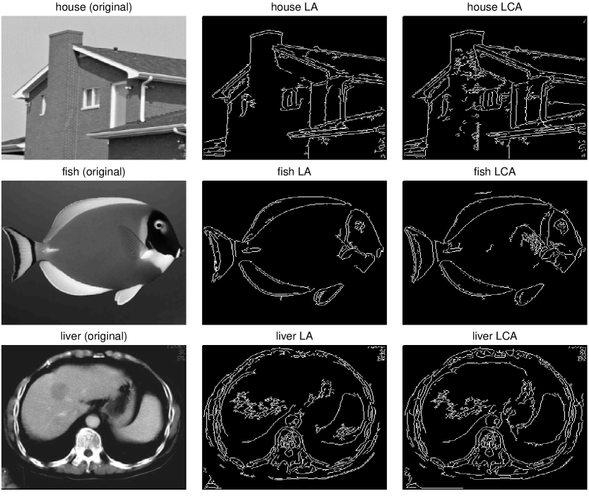
Figure 1: Edge detection results by LA and LCA.

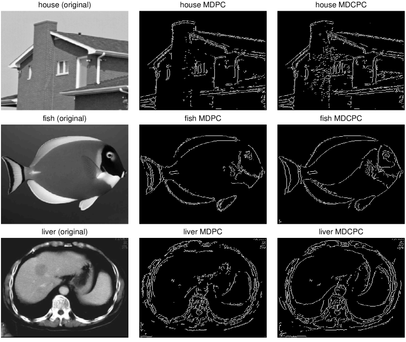
Figure 2: Edge detection results by MDPC and MDCPC.

References

• [1] M.Β Moshinsky and C.Β Quesne, β€œLinear canonical transformations and their unitary representations,” J. Math. Phys., vol.Β 12, no.Β 8, pp. 1772–1780, 1971.
• [2] J.Β J. Healy, M.Β A. Kutay, H.Β M. Ozaktas, and J.Β T. Sheridan, Linear Canonical Transforms.Β Β Β Springer, 2016.
• [3] S.Β Shinde, β€œTwo channel paraunitary filter banks based on linear canonical transform,” IEEE Transactions on Signal Processing, vol.Β 59, no.Β 2, pp. 832–836, 2011.
• [4] J.Β Shi, X.Β Liu, X.Β Sha, and N.Β Zhang, β€œSampling and reconstruction of signals in function spaces associated with the linear canonical transform,” IEEE Transactions on Signal Processing, vol.Β 60, no.Β 11, pp. 6041–6047, 2012.
• [5] Y.Β Fu and L.Β Li, β€œGeneralized analytic signal associated with linear canonical transform,” Optics Communications, vol. 281, no.Β 6, pp. 1468–1472, 2008.
• [6] F.Β Brackx, R.Β Delanghe, and F.Β Sommen, Clifford Analysis, ser. Research Notes in Mathematics.Β Β Β Boston, London, Melbourne: Pitman Advanced Publishing Company, 1982, vol.Β 76.
• [7] Y.Β Yang, K.Β I. Kou, and C.Β Zou, β€œEdge detection methods based on modified differential phase congruency of monogenic signal,” Multidimensional Systems and Signal Processing, pp. 1–21, 2017.